NBER WORKING PAPER SERIES

AN ELEMENTARY THEORY OF GLOBAL SUPPLY CHAINS

Arnaud CostinotJonathan Vogel

Su Wang

Working Paper 16936http://www.nber.org/papers/w16936

NATIONAL BUREAU OF ECONOMIC RESEARCH1050 Massachusetts Avenue

Cambridge, MA 02138April 2011

We thank Pol Antràs, Ariel Burstein, Bob Gibbons, Gene Grossman, Juan Carlos Hallak, Gordon Hanson,Elhanan Helpman, Oleg Itskhoki, Kiminori Matsuyama, Marc Melitz, Andrés Rodríguez-Clare, andseminar participants at Harvard University, Hitotsubashi University and the CESifo global economyconference. Costinot thanks the Alfred P. Sloan foundation for financial support. Vogel thanks theNational Science Foundation (under Grant SES-0962261) for research support. Any opinions, findings,and conclusions or recommendations expressed in this paper are those of the authors and do not necessarilyreflect the views of the National Science Foundation, the National Bureau of Economic Research,or any other organization.

NBER working papers are circulated for discussion and comment purposes. They have not been peer-reviewed or been subject to the review by the NBER Board of Directors that accompanies officialNBER publications.

© 2011 by Arnaud Costinot, Jonathan Vogel, and Su Wang. All rights reserved. Short sections of text,not to exceed two paragraphs, may be quoted without explicit permission provided that full credit,including © notice, is given to the source.

An Elementary Theory of Global Supply ChainsArnaud Costinot, Jonathan Vogel, and Su WangNBER Working Paper No. 16936April 2011JEL No. F1

ABSTRACT

This paper develops an elementary theory of global supply chains. We consider a world economywith an arbitrary number of countries, one factor of production, a continuum of intermediate goods,and one final good. Production of the final good is sequential and subject to mistakes. In the uniquefree trade equilibrium, countries with lower probabilities of making mistakes at all stages specializein later stages of production. Because of the sequential nature of production, absolute productivitydifferences are a source of comparative advantage among nations. Using this simple theoretical framework,we offer a first look at how vertical specialization shapes the interdependence of nations.

Arnaud CostinotDepartment of EconomicsMIT, E52-243B50 Memorial DriveCambridge MA 02142-1347and NBERcostinot@mit.edu

Jonathan VogelDepartment of EconomicsColumbia University420 West 118th StreetNew York, NY 10027and NBERjvogel@columbia.edu

Su WangMITsu_wang@mit.edu

�One man draws out the wire, another straights it, a third cuts it, a fourth

points it, a �fth grinds it at the top for receiving the head; to make the head

requires two or three distinct operations; to put it on, is a peculiar business, to

whiten the pins is another; it is even a trade by itself to put them into the paper;

and the important business of making a pin is, in this manner, divided into about

eighteen distinct operations, which, in some manufactories, are all performed by

distinct hands, though in others the same man will sometimes perform two or

three of them.�Adam Smith (1776)

1 Introduction

Most production processes consist of a large number of sequential stages. In this regard the

production of pins in late eighteenth century England is no di¤erent from today�s produc-

tion of tee-shirts, cars, computers, or semiconductors. Today, however, production processes

increasingly involve global supply chains spanning multiple countries, with each country spe-

cializing in particular stages of a good�s production sequence, a phenomenon which Hummels,

Ishii, and Yi (2001) refer to as vertical specialization.

This worldwide phenomenon has attracted a lot of attention among policy makers, busi-

ness leaders, and trade economists alike. On the academic side of this debate, a large

literature has emerged to investigate how the possibility to fragment production processes

across borders may a¤ect the volume, pattern, and consequences of international trade; see

e.g. Feenstra and Hanson (1996), Yi (2003), and Grossman and Rossi-Hansberg (2008). In

this paper, we propose to take a �rst look at a distinct, but equally important question:

Conditional on production processes being fragmented across borders, how does technologi-

cal change, either global or local, a¤ect di¤erent countries participating in the same supply

chain? In other words, how does vertical specialization shape the interdependence of nations?

From a theoretical standpoint, this is not an easy question. General equilibrium models

with an arbitrary number of goods and countries� with or without sequential production�

rarely provide sharp and intuitive comparative static predictions.1 In order to make progress,

we therefore start by proposing a simple theory of trade with sequential production. We

consider a world economy with multiple countries, one factor of production (labor), and one

�nal good. Production is sequential and subject to mistakes, as in Sobel (1992) and Kremer

(1993). Production of the �nal good requires a continuum of intermediate stages. At each of

these stages, production of one unit of an intermediate good requires one unit of labor and

one unit of the intermediate good produced in the previous stage. Mistakes occur along the

supply chain at a constant Poisson rate, which is an exogenous technological characteristic1Ethier (1984) o¤ers a review of theoretical results in high-dimensional trade models.

1

of a country. When a mistake occurs at some stage, the intermediate good is entirely lost.

By these stark assumptions, we aim to capture the more general idea that because of less

skilled workers, worse infrastructure, or inferior contractual enforcement, both costly defects

and delays in production are more likely in some countries than in others.

Section 3 describes the properties of the free trade equilibrium in our basic environment.

Although our model allows for any �nite number of countries and a continuum of stages,

the unique free trade equilibrium is fully characterized by a simple system of �rst-order non-

linear di¤erence equations. This system can be solved recursively by �rst determining the

assignment of countries to di¤erent stages of production and then computing the wages and

export prices sustaining that allocation as an equilibrium outcome. In our model, the free

trade equilibrium always exhibits vertical specialization: countries with a lower probability

of making mistakes, at all stages, specialize in later stages of production, where mistakes are

more costly. Because of the sequential nature of production, absolute productivity di¤erences

are a source of comparative advantage among nations.

Using this simple model, the rest of our paper o¤ers a comprehensive exploration of

how technological change, either global or local, a¤ects di¤erent countries participating in

the same global supply chain. Section 4 analyzes the consequences of global technological

change. We investigate how an increase in the length of production processes, which we

refer to as an increase in �complexity,�and a uniform decrease in failure rates worldwide,

which we refer to as �standardization,� may a¤ect the pattern of vertical specialization

and the world income distribution. Building solely on the idea that labor markets must

clear both before and after a given technological change, we demonstrate that although

both an increase in complexity and standardization lead all countries to �move up� the

supply chain, they have opposite e¤ects on inequality between nations. While an increase

in complexity increases inequality around the world, standardization bene�ts poor countries

disproportionately more. According to our model, standardization may even lead to a welfare

loss in the most technologically advanced country, a strong form of immiserizing growth.

Section 5 focuses on how local technological change may spill over, through terms-of-trade

e¤ects, to other countries participating in the same supply chain. We consider two forms

of local technological change: (i) labor-augmenting technical progress, which is isomorphic

to population growth; and (ii) a decrease in a country�s failure rate, which we refer to as

�routinization.� In a world with sequential production, we show that local technological

changes tend to spillover very di¤erently at the bottom and the top of the chain. At the

bottom, depending on the nature of technological changes, all countries either move up

or down, but whatever they do, movements along the chain fully determine changes in

inequality between nations. At the top of the chain, by contrast, local technological progress

always leads all countries to move up, but even conditioning on the nature of technological

2

change, inequality between nations may either fall or rise. Perhaps surprisingly, while richer

countries at the bottom of the chain bene�t disproportionately more from being pushed into

later stages of production, this is not always true at the top.

Section 6 demonstrates how more realistic features of global supply chains may easily

be incorporated into our simple theoretical framework. Our �rst extension introduces �co-

ordination costs� across countries. Among other things, we demonstrate that a decrease

in coordination costs may lead to �overshooting:�more stages of production may be o¤-

shored to a small country at intermediate levels of coordination costs than under perfectly

free trade. Our second extension allows for the existence of multiple parts, each produced

sequentially and then assembled, with equal productivity in each country, into a unique �nal

good using labor. In this environment, we show that the poorest countries tend to specialize

in assembly, while the richest countries tend to specialize in the later stages of the most

complex parts. Our �nal extension allows for heterogeneity in failure rates across di¤erent

stages. In this generalized version of our model, we provide su¢ cient conditions under which

our cross-sectional predictions remain unchanged.

Our paper is related to several strands of the literature. First, we draw some ideas from

the literature on hierarchies in closed-economy (and mostly partial-equilibrium) models. Im-

portant contributions include Lucas (1978), Rosen (1982), Sobel (1992), Kremer (1993),

Garicano (2000) and Garicano and Rossi-Hansberg (2006). As in Sobel (1992) and Kremer

(1993), we focus on an environment in which production is sequential and subject to mis-

takes, though we do so in a general equilibrium, open-economy setup. Models of hierarchies

have been applied to the study of international trade issues before, but with very di¤erent

goals in mind. For instance, Antràs, Garicano, and Rossi-Hansberg (2006) use the knowledge

economy model developed by Garicano (2000) to study the matching of agents with hetero-

geneous abilities across borders and its consequences for within-country inequality. Instead,

countries are populated by homogeneous workers in our model.2

In terms of techniques, our paper is also related to a growing literature using assignment or

matching models in an international context; see, for example, Grossman and Maggi (2000),

Grossman (2004), Yeaple (2005), Ohnsorge and Tre�er (2007), Blanchard and Willmann

(2010), Nocke and Yeaple (2008), Costinot (2009), and Costinot and Vogel (2010). Here, like

in some of our earlier work, we exploit the fact that the assignment of countries to stages

of production exhibits positive assortative matching� i.e., more productive countries are

assigned to later stages of production� in order to generate strong and intuitive comparative

static predictions in an environment with a large number of goods and countries.

In terms of focus, our paper is motivated by the recent literature documenting the impor-

2Other examples of trade papers using hierearchy models to study within-country inequality includeKremer and Maskin (2006), Sly (2010), Monte (2010), and Sampson (2010).

3

tance of vertical specialization in world trade. On the empirical side, this literature builds

on the in�uential work of Hummels, Rappoport, and Yi (1998), Hummels, Ishii, and Yi

(2001), and Hanson, Mataloni, and Slaughter (2005). Our focus on how vertical specializa-

tion shapes the interdependence of nations is also related to the work of Kose and Yi (2001,

2006), Burstein, Kurz, and Tesar (2008), and Bergin, Feenstra, and Hanson (2009) who

study how production sharing a¤ects the transmission of shocks at business cycle frequency.

On the theoretical side, the literature on fragmentation is large and diverse; see Antràs

and Rossi-Hansberg (2009) for a recent overview. Among existing papers, our theoretical

framework is most closely related to Dixit and Grossman (1982), Sanyal (1983), Yi (2003,

2010), Harms, Lorz, and Urban (2009), and Baldwin and Venables (2010) who also develop

trade models with sequential production. None of these papers, however, investigate how

technological change, either global or local, may di¤erentially impact countries located at

di¤erent stages of the same supply chain. This is the main focus of our analysis.

2 Basic Environment

We consider a world economy with multiple countries, indexed by c 2 C � f1; :::; Cg, onefactor of production, labor, and one �nal good. Labor is inelastically supplied and immobile

across countries. Lc and wc denote the endowment of labor and wage in country c, respec-

tively. Production of the �nal good is sequential and subject to mistakes. To produce the

�nal good, a continuum of stages s 2 S � (0; S] must be performed. At each stage, produc-ing one unit of intermediate good requires one unit of the intermediate good produced in the

previous stage and one unit of labor. For expositional purposes, we assume that �interme-

diate good 0�is in in�nite supply and has zero price.3 �Intermediate good S�corresponds

to the unique �nal good mentioned before.

Mistakes occur along the supply chain at a constant Poisson rate, �c > 0, which is an

exogenous technological characteristic of a country. It measures total factor productivity

(TFP) at any given stage of the production process. When a mistake occurs on a unit of

intermediate good at some stage, that intermediate good is entirely lost. Formally, if a �rm

from country c combines q(s) units of intermediate good s with q(s)ds units of labor, its

output of intermediate good s+ ds is given by

q (s+ ds) = (1� �cds) q (s) . (1)

3Alternatively, one could assume that �intermediate good 0�can be produced using labor only. In thissituation, the price of �intermediate good 0�would also be zero since only a measure zero of workers wouldbe required to perform this measure-zero set of stages. Assuming that �intermediate good 0�is in in�nitesupply allows us to avoid discussions of which country should produce this good. Such considerations areirrelevant for any of our results.

4

Note that letting q0 (s) � [q (s+ ds)� q (s)] =ds, Equation (1) can be written as q0 (s) =q (s) =��c. In other words, moving along the supply chain in country c, potential units of the �nalgood get destroyed at a constant rate, �c.

For technical reasons, we further assume that if a �rm produces intermediate good s+ds,

then it necessarily produces a positive measure of intermediate goods around that stage.4

This implies that each unit of the �nal good is produced by a �nite, though possibly arbi-

trarily large number of �rms. Countries are ordered such that �c is strictly decreasing in

c. Thus countries with a higher index c have higher total factor productivity. All markets

are perfectly competitive and all goods are freely traded. p(s) denotes the world price of

intermediate good s. We use the �nal good as our numeraire, p (S) = 1.

3 Free Trade Equilibrium

3.1 De�nition

In a free trade equilibrium, all �rms maximize their pro�ts taking world prices as given and

all markets clear. Pro�t maximization requires that for all c 2 C,

p (s+ ds) � (1 + �cds) p (s) + wcds,p (s+ ds) = (1 + �cds) p (s) + wcds, if Qc (s0) > 0 for all s0 2 (s; s+ ds],

(2)

where Qc (s0) denotes total output at stage s0 in country c. Condition (2) states that the

price of intermediate good s+ ds must be weakly less than its unit cost of production, with

equality if intermediate good s + ds is actually produced by a �rm from country c. To see

this, note that the production of one unit of intermediate good s+ ds requires 1= (1� �cds)units of intermediate good s as well as labor for all intermediate stages in (s; s + ds]. Thus

the unit cost of production of intermediate good s+ds is given by [p (s) + wcds] = (1� �cds).Since ds is in�nitesimal, this is equal to (1 + �cds)p (s) + wcds.

Good and labor market clearing further require that

PCc=1Qc (s2)�

PCc=1Qc (s1) = �

Z s2

s1

PCc=1 �cQc (s) ds, for all s1 � s2, (3)Z S

0

Qc (s) ds = Lc, for all c 2 C, (4)

Equation (3) states that the change in the world supply of intermediate goods between

stages s1 and s2 must be equal to the amount of intermediate goods lost due to mistakes in

4Formally, for any intermediate good s + ds, we assume the existence of s2 � s + ds > s1 such that ifq (s+ ds) > 0, then q (s0) > 0 for all s0 2 (s1; s2].

5

all countries between these two stages. Equation (4) states that the total amount of labor

used across all stages must be equal to the total supply of labor in country c. In the rest of

this paper, we formally de�ne a free trade equilibrium as follows.

De�nition 1 A free trade equilibrium corresponds to output levels Qc (�) : S �! R+ for allc 2 C, wages wc 2 R+ for all c 2 C, and intermediate good prices p (�) : S �! R+ such thatconditions (2)-(4) hold.

3.2 Existence and Uniqueness

We �rst characterize the pattern of international specialization in any free trade equilibrium.

Lemma 1 In any free trade equilibrium, there exists a sequence of stages S0 � 0 < S1 <

::: < SC = S such that for all s 2 S and c 2 C, Qc (s) > 0 if and only if s 2 (Sc�1; Sc].

According to Lemma 1, there is vertical specialization in any free trade equilibrium with

more productive countries producing and exporting at later stages of production. The formal

proof as well as all subsequent proofs can be found in the appendix.5 The intuition behind

Lemma 1 can be understood in two ways. One possibility is to look at Lemma 1 through the

lens of the hierarchy literature; see e.g. Lucas (1978), Rosen (1982), and Garicano (2000).

Since countries that are producing at later stages can leverage their productivity on larger

amounts of inputs, e¢ ciency requires countries to be more productive at the top. Another

possibility is to note that since new intermediate goods require both intermediate goods

produced in previous stages and labor, prices must be increasing along the supply chain.

Thus intermediate goods produced at later stages are less labor intensive, which makes them

relatively cheaper to produce in countries with higher wages. In our model these are the

countries with higher TFP at all stages. Because of the sequential nature of production,

absolute productivity di¤erences are a source of comparative advantage among nations.6

We refer to the vector (S1; :::; SC) as the �pattern of vertical specialization� and denote

by Qc � Qc (Sc) the total amount of intermediate good Sc produced and exported by country5A result similar to Lemma 1 in an environment with a discrete number of stages can also be found in

Sobel (1992) and Kremer (1993).6In his early work on fragmentation, Jones (1980) pointed out that if some factors of production are

internationally mobile, then absolute advantage may a¤ect the pattern of international specialization. Thebasic idea is that if physical capital is perfectly mobile and one country has an absolute advantage inproducing capital services, then it will specialize in capital intensive goods. The logic of our results isvery di¤erent and intimately related to the sequential nature of production. Mathematically, a simpleway to understand why sequential production processes make abolute productivity di¤erences a source ofcomparative advantage is to consider the cumulative amount of labor necessary to produce all stages from 0 tos � S for a potential unit of the �nal good. By equation (1), this is equal to e�cs which is log-supermodularin (�c; s). This is the exact same form of complementarity that determines the pattern of internationalspecializatin in standard Ricardian models; see Costinot (2009).

6

c. Using the previous notation, the pattern of vertical specialization and export levels can

be jointly characterized as follows.

Lemma 2 In any free trade equilibrium, the pattern of vertical specialization and exportlevels satisfy the following system of �rst-order non-linear di¤erence equations:

Sc = Sc�1 ��1

�c

�ln

�1� �cLc

Qc�1

�, for all c 2 C, (5)

Qc = e��c(Sc�Sc�1)Qc�1, for all c 2 C, (6)

with boundary conditions S0 = 0 and SC = S.

Lemma 2 derives from the goods and labor market clearing conditions (3) and (4). Equa-

tion (5) re�ects the fact that the exogenous supply of labor in country c must equal the

amount of labor demanded to perform all stages from Sc�1 to Sc. This amount of labor

depends both on the rate of mistakes �c as well as the total amount Qc�1 of intermediate

good Sc�1 imported from country c � 1. Equation (6) re�ects the fact that intermediategoods get lost at a constant rate at each stage when produced in country c.

In the rest of this paper, we refer to the vector of wages (w1; :::; wC) as the �world income

distribution� and to pc � p (Sc) as the price of country c�s exports (which is also the priceof country c + 1�s imports under free trade). Let Nc � Sc � Sc�1 denote the measure ofstages performed by country c within the supply chain. In the next lemma, we show that

the measures of stages being performed in all countries (N1; :::; NC) entirely summarize how

changes in the pattern of vertical specialization a¤ect the world income distribution.

Lemma 3 In any free trade equilibrium, the world income distribution and export pricessatisfy the following system of �rst-order linear di¤erence equations:

wc+1 = wc + (�c � �c+1) pc, for all c < C, (7)

pc = e�cNcpc�1 +�e�cNc � 1

�(wc=�c) , for all c 2 C, (8)

with boundary conditions p0 = 0 and pC = 1.

Lemma 3 derives from the zero-pro�t condition (2). Equation (7) re�ects the fact that

for the �cuto¤� good, Sc, the unit cost of production in country c, (1 + �cds) pc + wcds,

must be equal to the unit cost of production in country c + 1, (1 + �c+1ds) pc + wc+1ds.

Equation (8) directly derives from the zero-pro�t condition (2) and the de�nition of Nc and

pc. It illustrates the fact that the price of the last intermediate good produced by country

c depends on the price of the intermediate good imported from country c� 1 as well as thetotal labor cost in country c.

7

Combining Lemmas 1-3, we can establish the existence of a unique free trade equilibrium

and characterize its main properties.

Proposition 1 There exists a unique free trade equilibrium. In this equilibrium, the patternof vertical specialization and export levels are given by equations (5) and (6), and the world

income distribution and export prices are given by equations (7) and (8).

The proof of Proposition 1 formally proceeds in two steps. First, we use Lemma 2

to construct the unique pattern of vertical specialization and vector of export levels. In

equations (5) and (6), we have one degree of freedom, Q0, which corresponds to total input

used at the initial stage of production. Since SC is decreasing inQ0, it can be set to satisfy the

�nal boundary condition SC = S. Once (S1; :::; SC) and (Q0; :::; QC�1) have been determined,

all other output levels can be computed using equation (1) and Lemma 1. Second, we use

Lemma 3 together with the equilibrium measure of stages computed before, (N1; :::; NC), to

characterize the unique world income distribution and vector of export prices. In equations

(7) and (8), we still have one degree of freedom, w1. Given the monotonicity of pC in w1, it

can be used to satisfy the other �nal boundary condition, pC = 1. Finally, once (w1; :::; wC)

and (p1; :::; pC) have been determined, all other prices can be computed using the zero-pro�t

condition (2) and Lemma 1.

3.3 Discussion

As a �rst step towards analyzing how vertical specialization shapes the interdependence of

nations, we have provided a full characterization of free trade equilibria in a simple trade

model with sequential production. Before turning to our comparative static exercises, we

brie�y discuss the cross-sectional implications that have emerged from this characterization.

First, since rich countries specialize in later stages of production while poor countries

specialize in earlier stages, our model implies that rich countries tend to trade relatively

more with other rich countries (from whom they import their intermediates and to whom

they export their output) while poor countries tend to trade relatively more with other poor

countries, as documented by Hallak (2010). Second, since intermediate goods produced in

later stages have higher prices and countries producing in these stages have higher wages,

our model implies that rich countries both tend to import goods with higher unit values, as

documented by Hallak (2006), and to export goods with higher unit values, as documented

by Schott (2004), Hummels and Klenow (2005), and Hallak and Schott (2010).

Following Linder (1961), the two previous stylized facts have traditionally been ratio-

nalized using non-homothetic preferences; see e.g. Markusen (1986), Flam and Helpman

(1987), Bergstrand (1990), Stokey (1991), Murphy and Shleifer (1997) Matsuyama (2000),

8

Fieler (2010), and Fajgelbaum, Grossman, and Helpman (2009). The common starting point

of the previous papers is that rich countries�preferences are skewed towards high quality

goods, so they tend to import goods with higher unit values. Under the assumption that

rich countries are also relatively better at producing high quality goods, these models can

further explain why rich countries tend to export goods with higher unit values and why

countries with similar levels of GDP per capita tend to trade more with each other.7

The complementary explanation o¤ered by our elementary theory of global supply chains

is based purely on supply considerations. According to our model, countries with similar

per-capita incomes are more likely to trade with one another because they specialize in

nearby regions of the same supply chain. Similarly, countries with higher levels of GDP

per capita tend to have higher unit values of imports and exports because they specialize

in higher stages in the supply chain, for which inputs and outputs are more costly. Note

that our supply-side explanation also suggests new testable implications. Since our model

only applies to sectors characterized by sequential production and vertical specialization,

if our theoretical explanation is empirically relevant, one would therefore expect �Linder

e¤ects�� i.e. the extent of trade between countries with similar levels of GDP per capita�

to be higher, all else equal, in sectors in which production processes are vertically fragmented

across borders in practice.

The previous cross-sectional predictions, of course, should be interpreted with caution.

Our theory is admittedly very stylized. In Section 6, we will discuss how the previous results

may be a¤ected (or not) by the introduction of more realistic features of global supply chains.

4 Global Technological Change

Many technological innovations, from the discovery of electricity to the internet, have im-

pacted production processes worldwide. Our �rst series of comparative static exercises fo-

cuses on the impact of global technological changes on di¤erent countries participating in

the same supply chain. Our goal is to investigate how an increase in the length of production

processes, perhaps associated with the development of higher quality goods, as well as a uni-

form decrease in failure rates worldwide, perhaps due to the standardization of production

processes, may a¤ect the pattern of vertical specialization and the world income distribution.

7In Fajgelbaum, Grossman, and Helpman (2009), such predictions are obtained in the absence of anyexogenous relative productivity di¤erences. In their model, a higher relative demand for high-quality goodstranslates into a higher relative supply of these goods through a �home-market�e¤ect.

9

4.1 De�nitions

It is useful to introduce �rst some formal de�nitions describing the changes in the pattern

of vertical specialization and the world income distribution in which we will be interested.

De�nition 2 Let (S 01; :::; S0C) denote the pattern of vertical specialization in a counterfactual

free trade equilibrium. A country c 2 C is moving up (resp. down) the supply chain relative tothe initial free trade equilibrium if S 0c � Sc and S 0c�1 � Sc�1 (resp. S 0c � Sc and S 0c�1 � Sc�1).

According to De�nition 2, a country is moving up or down the supply chain if we can

rank the set of stages that it performs in the initial and counterfactual free trade equilibria

in terms of the strong set order. Among other things, this simple mathematical notion will

allow us to formalize a major concern of policy makers and business leaders in developed

countries, namely the fact that China and other developing countries are �moving up the

value chain;�see e.g. OECD (2007).

De�nition 3 Let (w01; :::; w0C) denote the world income distribution in a counterfactual free

trade equilibrium. Inequality is increasing (resp. decreasing) among a given group fc1; :::cngof adjacent countries if w0c+1=w

0c � wc+1=wc (resp. w0c+1=w0c � wc+1=wc) for all c1 � c � cn�1.

According to De�nition 3, inequality is increasing (resp. decreasing) within a given group

of adjacent countries, if for any pair of countries within that group, the relative wage of the

richer country is increasing (resp. decreasing). Since wages correspond to GDP per capita

in our model, this property o¤ers a simple way to conceptualize changes in the world income

distribution.

4.2 Increase in complexity

At the end of the eighteenth century, Adam Smith famously noted that making a pin was

divided into about 18 distinct operations. Today, as mentioned by Levine (2010), making a

Boeing 747 requires more than 6,000,000 parts, each of them requiring many more operations.

In this section we analyze the consequences of an increase in the measure of stages S necessary

to produce a �nal good, which we simply refer to as an �increase in complexity.�8

Our approach, like in subsequent sections, proceeds in two steps. We characterize �rst

the changes in the pattern of vertical specialization and second the associated changes in the

world income distribution. Our �rst comparative static results can be stated as follows.

8For expositional purposes, we abstract from any utility gains that may be associated with the productionof more complex goods in practice. Our analytical results on the pattern of vertical specialization and theinequality between nations do not depend on this simpli�cation. But it should be clear that changes in realwages, which will necessarily decrease after an increase in complexity, crucially depend on it.

10

1 1.5 2 2.50

0.5

1

1.5

2

2.5

3

S

Sta

ges

0.5 1 1.5 2 2.5 30

0.2

0.4

0.6

0.8

1

1.2

1.4

1.6

1.8

2

SW

ages

(S4,S5]

(S3,S4]

(S2,S3]

(S1,S2]

(S0,S1]

w5w4w3w2w1

C=5, (L1,λ1)=(0.55,0.78), (L 2,λ2)=(0.30,0.63), (L 3,λ3)=(0.74,0.37), (L 4,λ4)=(0.19,0.18), (L 5,λ5)=(0.69,0.08)

Figure 1: Consequences of an increase in complexity.

Proposition 2 An increase in complexity leads all countries to move up the supply chainand increases inequality between countries around the world.

The changes in the pattern of vertical specialization and the world income distribution

associated with an increase in complexity are illustrated in Figure 1. The broad intuition

behind changes in the pattern of vertical specialization is simple. An increase in complexity

tends to decrease total output at all stages of production. Since labor supply must remain

equal to labor demand, this decrease in output levels must be accompanied by an increase

in the measure Nc of stages performed in all countries. Proceeding by iteration from the

bottom of the supply chain, we can then show that this change in Nc can only occur if all

countries move up.

The logic behind the changes in the world income distribution is more subtle. From

Lemma 3, we know that relative wages satisfy

wc+1wc

= 1 +�c � �c+1(wc=pc)

, for all c < C. (9)

Thus, wc+1=wc is decreasing in the labor intensity, wc=pc, of country c�s export. From the

�rst part of Proposition 2, we also know that countries: (i) are performing more stages,

which tends to increase export prices (for a given price of imported inputs); and (ii) are

moving up into higher stages, which tend to have higher export prices (for a given schedule

11

of prices). Both e¤ects tend to raise the price of intermediate goods that are being traded,

and in turn, to decrease their labor intensity. This explains why inequality between nationsincreases. This e¤ect is reminiscent of the mechanism underlying terms-of-trade e¤ects in a

Ricardian model; see e.g. Dornbusch, Fischer, and Samuelson (1977) and Krugman (1986).

From an economic standpoint, equation (9) captures the basic idea that the wage of country

c+1 should increase relative to the wage of country c if and only if c+1 moves into sectors

in which it has a comparative advantage. In our model, since country c + 1 has a higher

wage, these are the sectors with lower labor intensities. In a standard Ricardian model, these

would be the sectors in which country c+ 1 is relatively more productive instead.

There is, however, one important di¤erence between our model with sequential production

and a standard Ricardian model. In our model, the pattern of comparative advantage

depends on endogenous di¤erences in labor intensity across stages. In a standard Ricardian

model, the same pattern only depends on exogenous productivity di¤erences. As we will

see in Section 5.1, this subtle distinction may lead to very di¤erent predictions about the

consequences of technological change on inequality between nations.9

4.3 Standardization

In most industries, production processes become more standardized as goods mature over

time. In order to study the potential implications of this particular type of technological

change within our theoretical framework, we now consider a uniform decrease in failure rates

from �c to �0c � ��c for all c 2 C, with � < 1, which we simply refer to as �standardization.�

The consequences of standardization on the pattern of vertical specialization and the world

income distribution can be described as follows.

Proposition 3 Standardization leads all countries to move up the supply chain and de-creases inequality between countries around the world.

The consequences of standardization are illustrated in Figure 2. For a given pattern

of vertical specialization, standardization tends to raise total output� and, therefore, the

demand for labor� at all stages of production. Since labor supply must remain equal to

labor demand, this increase in output levels must be partially o¤set by a reduction of output

at earlier stages of production. Hence, poor countries must increase the measure of stages

that they perform, pushing all countries up the supply chain.

9While the previous results emphasize the consequences of an increase in the complexity of productionprocesses on inequality between nations, it is worth pointing out that Proposition 2 also provides microthe-oretical foundations for a novel form of skill-biased technological change within nations. In a world withsequential production, our results demonstrate that the introduction of new stages of production tend tobene�t skilled workers disproportionately more, even if new stages are not skill-biased per se.

12

1 2 3 40

0.1

0.2

0.3

0.4

0.5

0.6

0.7

0.8

0.9

1

1/β

Sta

ges

0 1 2 3 4 50.5

0.6

0.7

0.8

0.9

1

1.1

1/βW

ages

(S4,S5]

(S3,S4]

(S2,S3]

(S1,S2]

(S0,S1]

w5w4w3w2w1

C=5, (L1,λ1)=(0.53,0.97), (L 2,λ2)=(0.65,0.61), (L 3,λ3)=(0.41,0.53), (L 4,λ4)=(0.82,0.33), (L 5,λ5)=(0.72,0.11)

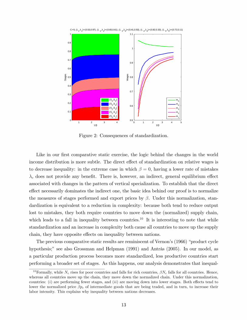
Figure 2: Consequences of standardization.

Like in our �rst comparative static exercise, the logic behind the changes in the world

income distribution is more subtle. The direct e¤ect of standardization on relative wages is

to decrease inequality: in the extreme case in which � = 0, having a lower rate of mistakes

�c does not provide any bene�t. There is, however, an indirect, general equilibrium e¤ect

associated with changes in the pattern of vertical specialization. To establish that the direct

e¤ect necessarily dominates the indirect one, the basic idea behind our proof is to normalize

the measures of stages performed and export prices by �. Under this normalization, stan-

dardization is equivalent to a reduction in complexity: because both tend to reduce output

lost to mistakes, they both require countries to move down the (normalized) supply chain,

which leads to a fall in inequality between countries.10 It is interesting to note that while

standardization and an increase in complexity both cause all countries to move up the supply

chain, they have opposite e¤ects on inequality between nations.

The previous comparative static results are reminiscent of Vernon�s (1966) �product cycle

hypothesis;� see also Grossman and Helpman (1991) and Antràs (2005). In our model, as

a particular production process becomes more standardized, less productive countries start

performing a broader set of stages. As this happens, our analysis demonstrates that inequal-

10Formally, while Nc rises for poor countries and falls for rich countries, �Nc falls for all countries. Hence,whereas all countries move up the chain, they move down the normalized chain. Under this normalization,countries: (i) are performing fewer stages, and (ii) are moving down into lower stages. Both e¤ects tend tolower the normalized price �pc of intermediate goods that are being traded, and in turn, to increase theirlabor intensity. This explains why inequality between nations decreases.

13

ity between nations decreases around the world. Figure 2 also illustrates that although the

direct e¤ect of standardization is to increase output in all countries, welfare may fall in the

most technologically advanced countries through a terms-of-trade deterioration. This is rem-

iniscent of Bhagwati�s (1958) �immiserizing growth.�Two key di¤erences, however, need to

be highlighted. First, standardization proportionately increases TFP in all countries in the

global supply chain, whereas Bhagwati�s (1958) immiserizing growth occurs in response to an

outward shift in the production possibility frontier in one country. Second, standardization

proportionately increases TFP at all stages of production, whereas Bhagwati�s (1958) im-

miserizing growth occurs in response to an outward shift in the export sector. In our model,

it is the sequential nature of production that makes uniform TFP growth endogenously act

as export-biased technological change in the more technologically advanced countries.11

5 Local Technological Change

Two of the major changes in today�s world economy are: (i) the increased fragmentation

of the production process, which Baldwin (2006) refers to as the �Great Unbundling;�and

(ii) the rise of China and other developing countries, such as India and Brazil. While both

phenomena have been studied separately, we know very little about their interaction. The

goal of this section is to use our elementary theory of global supply chains to shed light on

this issue. To do so, our second series of comparative static exercises focuses on the impact

of labor-augmenting technical progress and routinization in one country and describes how

they �spill over�to other countries in the same supply chain through terms-of-trade e¤ects.

5.1 Labor-augmenting technical progress

We �rst study the impact of labor-augmenting technical progress, which is isomorphic to

an increase in the total endowment of labor, Lc0, of a given country c0. Following the same

two-step logic as in Section 4, the consequences of labor-augmenting technical progress can

be described as follows.

Proposition 4 Labor-augmenting technical progress in country c0 leads all countries c < c0to move down the supply chain and all countries c > c0 to move up. This decreases inequality

among countries c 2 f1; :::; c0g, increases inequality among countries c 2 fc0; :::; c1g, anddecreases inequality among countries c 2 fc1; :::; Cg, with c1 2 fc0 + 1; :::; Cg.11Like in Bhagwati�s original paper, however, it should be clear that immiserizing growth arises in this

environment because of strong complementarities between goods. In our model, producing one unit ofintermediate good always requires one unit of the intermediate good produced in the previous stage and oneunit of labor. This explains why technological changes may have large (and adverse) terms-of-trade e¤ects.

14

1 2 3 4 5 60

0.1

0.2

0.3

0.4

0.5

0.6

0.7

0.8

0.9

1

L3

Stag

es

0 2 4 6 80.7

0.75

0.8

0.85

0.9

0.95

1

1.05

L3W

ages

(S4,S5]

(S3,S4]

(S2,S3]

(S1,S2]

(S0,S1]

w5w4w3w2w1

C=5, (L1,λ1)=(0.28,0.96), (L 2,λ2)=(0.68,0.59), (L 3,λ3)=(0.66,0.50), (L 4,λ4)=(0.16,0.34), (L 5,λ5)=(0.12,0.22)

Figure 3: Consequences of labor-augmenting technical progress in country 3.

The spillover e¤ects associated with labor-augmenting technical progress are illustrated

in Figure 3. The broad intuition behind changing patterns of specialization is simple. An

increase in the supply of labor (in e¢ ciency units) in one country tends to raise total output

at all stages of production. Since labor supply must remain equal to labor demand, this

increase in output levels must be accompanied by a decrease in the measure of stages Ncperformed in each country c 6= c0. Proceeding by iteration from the bottom and the top of

the supply chain, we can then show that this change in Nc can only occur if all countries

below c0 move down and all countries above c0 move up. Finally, since the total measure

of stages must remain constant, the measure of stages Nc0 performed in country c0 must

increase.

Changes in the pattern of vertical specialization naturally translate into changes in the

world income distribution. As in Section 4.2, countries at the bottom of the chain are mov-

ing down into lower stages and are performing fewer stages. Both e¤ects tend to decrease

inequality between nations at the bottom of the chain. The non-monotonic e¤ects on in-

equality at the top of the chain re�ect two con�icting forces. On the one hand, countries are

moving up, which tends to increase the price of intermediate goods traded in that region of

the supply chain, and in turn, to decrease their labor intensity. On the other hand, countries

are performing fewer stages, which tends to reduce the price of their exports and increase

15

their labor intensity.12

The previous non-monotonic e¤ects stand in sharp contrast to the predictions of standard

Ricardian models and illustrate nicely the importance of modeling the sequential nature of

production for understanding the consequences of technological changes in developing and

developed countries on their trading partners worldwide. To see this, consider a Ricardian

model without sequential production in which there is a ladder of countries with poor coun-

tries at the bottom and rich countries at the top. Krugman (1986) is a well-known example.

In such an environment, if foreign labor-augmenting technical progress leads the richest

countries to move up, inequality among these countries necessarily increases. The reason is

simple. On the one hand, the relative wage of two adjacent countries is equal to their relative

productivity in the �cuto¤�sector. On the other hand, richer countries are relatively more

productive in sectors higher up the ladder (otherwise they would not be specializing in these

sectors in equilibrium). By contrast, Proposition 4 predicts that as the richest countries

move up, inequality may decrease at the very top of the chain. This counterintuitive result

derives from the fact that the pattern of comparative advantage in a model with sequential

production is not exogenously given, but depends instead on endogenous factor prices. This

subtle distinction breaks the monotonic relationship between the pattern of international

specialization and inequality between nations. Although later stages are necessarily less la-

bor intensive in a given equilibrium, the labor intensity of later stages in the new equilibrium

may be higher than the labor intensity of earlier stages in the initial equilibrium. At the

top of the chain, poorer countries may therefore bene�t disproportionately more from being

pushed into later stages of production.

5.2 Routinization

We now turn our attention to the consequences of a decrease in the failure rate �c0 of a

given country c0, which we refer to as �routinization.�For simplicity we restrict ourselves to

a small change in �c0, in the sense that it does not a¤ect the ranking of countries in terms

of failure rates. The consequences of routinization can be described as follows.

Proposition 5 Routinization in country c0 leads all countries move up the supply chain,increases inequality among countries c 2 f1; :::; c0g, decreases inequality among countriesc 2 fc0; c0 + 1g, increases inequality among countries c 2 fc0 + 1; :::; c1g, and decreasesinequality among countries c 2 fc1; :::; Cg, with c1 2 fc0 + 1; :::; Cg.

The spillover e¤ects associated with routinization are illustrated in Figure 4. According

to Proposition 5, all countries move up the supply chain. In this respect, the consequences12Note that since c1 2 fc0 + 1; :::; Cg, the third group of countries, fc1; :::; C � 1g, is non-empty if c1 < C,

but empty if c1 = C. We have encountered both cases in our simulations.

16

0.65 0.7 0.75 0.80

0.1

0.2

0.3

0.4

0.5

0.6

0.7

0.8

0.9

1

1/λ3

Stag

es

0.65 0.7 0.75 0.8 0.850.4

0.45

0.5

0.55

0.6

0.65

1/λ3W

ages

(S4,S5]

(S3,S4]

(S2,S3]

(S1,S2]

(S0,S1]

w5w4w3w2w1

C=5, (L1,λ1)=(1.29,1.88), (L 2,λ2)=(0.76,1.75), (L 3,λ3)=(1.62,1.25), (L 4,λ4)=(1.07,1.17), (L 5,λ5)=(0.70,1.10))

Figure 4: Consequences of routinization in country 3.

of routinization are the same as the consequences of labor-augmenting technical progress at

the top of the chain, but the exact opposite at the bottom.

To understand this result, consider �rst countries located at the top of the chain. Since

total output of the �nal good must rise in response to a lower failure rate in country c0,

countries at the top of the chain must perform fewer stages for labor markets to clear.

By a simple iterative argument, these countries must therefore move further up the supply

chain, just like in Proposition 4. At the top of the chain, the consequences of routinization

for inequality are the same as the consequences of labor-augmenting technical progress. The

non-monotonicity� with inequality rising among countries c 2 fc0 + 1; :::; c1g and decreasingamong countries c 2 fc1; :::; Cg� arises from the same two con�icting forces: countries moveup the chain but produce fewer stages.

At the bottom of the chain, the broad intuition behind the opposite e¤ects of labor-

augmenting technical progress and routinization for changes in the pattern of specialization

can be understood as follows. Holding the pattern of vertical specialization �xed, labor-

augmenting technical progress in country c0 increases the total labor supply of countries

c � c0, but leaves their labor demand unchanged. Thus labor market clearing requires

countries at the bottom of the chain to reduce the number of stages they perform, to move

down the chain, and to increase their output, thereby o¤setting the excess labor supply at the

top. By contrast, routinization in country c0 increases the total labor demand of countries

17

c � c0 (since country c0 now produces more output at each stage), but leaves their labor

supply unchanged. As a result, countries at the bottom of the chain now need to increase

the number of stages they perform, to move up the chain, and to reduce their output in

order to o¤set the excess labor demand at the top. The consequences for inequality follow

from the same logic as in the previous section.13

Our goal in this section was to take a �rst stab at exploring theoretically the relationship

between vertical specialization and the recent emergence of developing countries like China.

A key insight that emerges from our analysis is that because of sequential production, local

technological changes tend to spillover very di¤erently at the bottom and the top of the chain.

At the bottom of the chain, depending on the nature of technological changes, countries may

move up or down, but whatever they do, movements along the chain fully determine changes

in the world income distribution within that region. At the top of the chain, by contrast,

local technological progress always leads countries to move up, but even conditioning on

the nature of technological change, inequality between nations within that region may fall

or rise. Perhaps surprisingly, while richer countries at the bottom of the chain bene�t

disproportionately more from being pushed into later stages of production, this is not always

true at the top. In fact, as Figure 4 illustrates, the most technologically advanced countries

may be the only ones losing as all countries move up around the world.

6 Extensions

Our elementary theory of global supply chains is special along several dimensions. First, all

intermediate goods are freely traded. Second, production is purely sequential. Third, stages

of production are identical in all dimensions except the order in which they are performed.

In this section we demonstrate how more realistic features of global supply chains may be

easily incorporated into our theoretical framework.

6.1 Coordination Costs

An important insight of the recent trade literature is that changes in trade costs a¤ect the

pattern and consequences of international trade not only by a¤ecting �nal goods trade, but

also by a¤ecting the extent of production fragmentation across borders; see e.g. Feenstra and

Hanson (1996), Yi (2003), and Grossman and Rossi-Hansberg (2008). We now discuss how

13The only di¤erence is that in the middle of the chain, inequality decreases among countries c 2fc0; c0 + 1g because of the direct e¤ect of a reduction in �c0 , which tends to decrease inequality between c0and c0+1, as seen in equation (9). This force was absent from our previous comparative static exercise sincelabor endowments (in e¢ ciency units) did not directly a¤ect zero pro�t conditions.

18

the introduction of trading frictions in our simple environment would a¤ect the geographic

structure of global supply chains, and in turn, the interdependence of nations.

A natural way to introduce trading frictions in our model is to assume that the likelihood

of a defect in the �nal good is increasing in the number of times the intermediate goods used

in its production have crossed a border. We refer to such costs, which are distinct from

standard iceberg trade costs, as �coordination costs.� Formally, if the production of one

unit of the �nal good in a given country involves n international transactions� i.e. export

and import at stages 0 < s1 � s2 � ::: � sn < S� then the �nal good is worthless with

probability 1 � �n 2 [0; 1]. The case considered in Section 2 corresponds to � = 1. Like inSection 2, we assume that the �nal good is freely traded and use it as our numeraire. Finally,

we assume that all international transactions are perfectly observable by all �rms so that

two units of the same intermediate good s may, in principle, command two di¤erent prices

if their production requires a di¤erent number of international transactions. Accordingly,

competitive equilibria remain Pareto optimal in the presence of coordination costs.

The analysis of this generalized version of our model is considerably simpli�ed by the fact

that, in spite of coordination costs, a weaker version of vertical specialization must still hold

in any competitive equilibrium. Let Cu (s) denote the country in which stage s has been

performed for the production of a given unit u. Using the previous notation, the pattern of

international specialization can be characterized as follows.

Lemma 4 In any competitive equilibrium, the allocation of stages to countries, Cu : S ! C,

is increasing in s for all u 2�0; QW �

Pc2C Qc (S)

�.

According to Lemma 4, for any unit of the �nal good, production must still involve vertical

specialization, with less productive countries specializing in earlier stages of production.

This result is weaker, however, than the one derived in Section 2 in that it does not require

Cu (�) to be the same for all units. This should be intuitive. Consider the extreme casein which coordination costs are in�nitely large. In this situation all countries will remain

under autarky in a competitive equilibrium. Thus the same stages of production will be

performed in di¤erent countries. In the presence of coordination costs, one can therefore only

expect vertical specialization to hold within each supply chain, whether or not all chains are

identical, which is what Lemma 4 establishes. Armed with Lemma 4, we can characterize

competitive equilibria using the same approach as in Section 2. The only di¤erence is that

we now need to guess �rst the structure of the equilibrium (e.g. some units are produced

entirely in country 1, whereas all other units are produced jointly in all countries) and then

verify ex post that our guess is correct.

Figure 5 illustrates how the structure of competitive equilibria varies with the magnitude

19

0.9 0.92 0.94 0.96 0.980

0.1

0.2

0.3

0.4

0.5

0.6

0.7

0.8

0.9

1

δ

Stag

es

Country 1Country 2Countries 1 & 2

0.9 0.92 0.94 0.96 0.98 10.7

0.75

0.8

0.85

0.9

0.95

δW

ages

w1w2

C=2, (L1,λ1)=(0.12,0.66), (L 2,λ2)=(0.50,0.16)

Figure 5: Consequences of a reduction in coordination costs.

of coordination costs in the two-country case.14 There are three distinct regions. For su¢ -

ciently high coordination costs, all stages are being performed in both countries and there is

no trade. Conversely, for low enough coordination costs, the pattern of vertical specialization

is the same as under free trade. In this region, reductions in coordination costs have no e¤ect

on the pattern of specialization, but raise wages in all countries. The most interesting case

arises when coordination costs are in an intermediate range. In this region, the large country

(country 2) is incompletely specialized, whereas the small country (country 1) is completely

specialized in a subset of stages. As can easily be shown analytically, the set of stages that

are being o¤shored to the small country is necessarily increasing in the level of coordination

costs over that range. Hence starting from autarky and decreasing coordination costs, there

will be �overshooting:� a broader set of stages will be performed in the poor country at

intermediate levels of coordination costs than under perfectly free trade. This pattern of

overshooting does not arise from coordination failures, heterogeneity in trade costs, or the

imperfect tradability of the �nal good, as discussed in Baldwin and Venables (2010). It

simply re�ects the fact that in a perfectly competitive model with sequential production and

trading frictions, a su¢ ciently large set of stages must be performed in the small country for

�rms to �nd it pro�table to fragment production across borders. Accordingly, the larger the

coordination costs, the larger the set of stages being performed in the small country!

14Details about the construction of these competitive equilibria are available upon request.

20

Figure 5 also illustrates that sequential production does not hinder the ability of smaller

countries to bene�t from international trade. On the contrary, smaller countries tend to

bene�t more from freer trade. In the above example, a decrease in coordination costs either

only bene�ts the small country (for intermediate levels of coordination costs) or a¤ects

real wages in both countries in the same proportional manner (for low enough coordination

costs). Finally, Figure 5 highlights that how many stages of the production process are

being o¤shored to a poor country may be a very poor indicator of the interdependence of

nations. Here, when the measure of stages being o¤shored is the largest, the rich country is

completely insulated from (small) technological shocks in the poor country.

6.2 Simultaneous Production of Multiple Parts and Assembly

Most production processes are neither purely sequential, as assumed in Section 2, nor purely

simultaneous, as assumed in most of the existing literature. Producing an aircraft, for

example, requires multiple parts, e.g. an engine, seats, and windows. These parts are

produced simultaneously before being assembled, but each of these parts requires a large

number of sequential stages, e.g. extraction of raw materials, re�ning, and manufacturing.15

With this is mind, we turn to a generalization of our original model in which there are

multiple supply chains, indexed by n 2 N � f1; :::; Ng, each associated with the productionof a part. We allow supply chains to di¤er in terms of their complexity, Sn, but for simplicity,

we require failure rates to be constant across chains and given by �c, as in Section 2. Hence

countries do not have a comparative advantage in particular parts. Parts are ordered such

that Sn is weakly increasing in n. So parts with a higher index n are more complex.

Parts are assembled into a unique �nal good using labor. Formally, the output Yc of the

�nal good in country c is given by

Yc = F�X1c ; :::; X

Nc ; Ac

�,

where F (�) is a production function with constant returns to scale, Xnc is the amount of

part n used in the production of the �nal good in country c, and Ac � Lc corresponds to

the amount of labor used for assembly in country c. Note that the production function

F (�) is assumed to be identical across countries, thereby capturing the idea that assembly issu¢ ciently standardized for mistakes in this activity to be equally unlikely in all countries.

Note also that by relabelling each part n as a distinct �nal good and the production function

F (�) as a utility function, with F (�) independent of Ac, this section can also be interpretedas a multi-sector extension of our baseline framework.16

15Manufacturing itself, of course, requires a large number of sequential stages.16More generally, one could interpret the present model as a multi-sector economy with one �outside�

21

In this generalized version of our model, the pattern of international specialization still

takes a very simple form, as the next lemma demonstrates.

Lemma 5 In any free trade equilibrium, there exists a sequence of stages S0 � 0 � S1 �::: � SC = SN such that for all n 2 N , s 2 [0; Sn], and c 2 C, Qnc (s) > 0 if and only if

s 2 (Sc�1; Sc]. Furthermore, if country c is engaged in parts production, Ac < Lc, then allcountries c0 > c are only involved in parts production, Ac0 = 0.

Lemma 5 imposes three restrictions on the pattern of international specialization. First,

the poorest countries tend to specialize in assembly, while the richest countries tend to

specialize in parts production. This directly derives from the higher relative productivity

of the poorest countries in assembly. Second, amongst the countries that produce parts,

richer countries produce and export at later stages of production. This result also held in

Section 3, and the intuition is unchanged. Third, whereas middle-income countries tend to

produce all parts, the richest countries tend to specialize in only the most complex ones.

Intuitively, even the �nal stage Sn of a simple part is su¢ ciently labor intensive that high-

wage, high-productivity countries are less competitive at that stage. Viewed through the

lens of the hierarchy literature, the �nal output of a simple chain does not embody a large

enough amount of inputs to merit, from an e¢ ciency standpoint, leveraging the productivity

of the most productive countries.

Compared to the simple model analyzed in Section 3, the present model suggests ad-

ditional cross-sectional predictions. Here, trade is more likely to be concentrated among

countries with similar levels of GDP per capita if exports and imports tend to occur along

the supply chain associated with particular parts rather than at the top between �part pro-

ducers� and �assemblers.�Accordingly, one should expect trade to be more concentrated

among countries with similar levels of GDP per capita in industries in which the production

process consists of very complex parts.

While cross-sectional predictions are potentially distinct from those of our simple model,

the logic underlying the interdependence of nations is very similar. Since we still have vertical

specialization in equilibrium, the free trade equilibrium remains characterized by a simple

system of non-linear di¤erence equations, akin to the ones presented in Lemmas 2 and 3. It

therefore remains fairly easy to analyze the consequences of technological change. The key

di¤erence between the present environment and the one considered in Sections 4 and 5 is

that the amount of labor allocated to vertical supply chains is now an endogenous variable

that depends on the amount of labor necessary for assembly.

good, that can be produced one-to-one from labor in all countries, and multiple �sequential�goods, whoseproduction is as described in Section 2. Under this interpretation, Ac would simply be the amount of laborallocated to the outside good in country c.

22

6.3 Heterogeneous Stages of Production

In order to focus attention in the simplest possible way on the novel aspects of an environment

with sequential production, we have assumed that stages of production only di¤er in one

dimension: the order in which they are performed. In practice, stages of production often

di¤er greatly in terms of factor intensity, with some stages being much more skill-intensive

than others. To capture such considerations within our simple theoretical framework, we

now allow failure rates to be an exogenous characteristic of both a stage and a country.

Formally, we assume that mistakes occur at a Poisson rate, �c(s), where �c(s) is: (i)

strictly decreasing in c, (ii) continuous and weakly increasing in s, and (iii) weakly submod-

ular in (s; c). This last restriction captures the idea that more e¢ cient countries also tend

to be the countries with a comparative advantage in later stages of production. Accordingly,

one can now think of s as a measure of skill intensity in the sense that higher stages are

associated with higher relative productivity in countries with more skilled workers, i.e. those

with lower failure rates at all stages.

As we demonstrate in the appendix, the pattern of international specialization in this

generalized version of our model is still characterized by Lemma 1. Our cross-sectional pre-

dictions are therefore unchanged: there is vertical specialization in any free trade equilibrium,

with more productive countries specializing in later stages of production. The intuition is

simple. Absent any comparative advantage across stages, we know that more productive

countries specialize in later stages of production. When �c(s) is submodular, the previous

pattern of international specialization is simply reinforced by the comparative advantage of

more productive countries in later stages.

The basic forces that determine the interdependence of nations remain the same as in

Sections 4 and 5. In particular, one can still show analytically that labor-augmenting techni-

cal progress in country c0 still leads all countries c < c0 to move down the supply chain and

all countries c > c0 to move up, just like in Proposition 4. The analysis of the consequences of

technological change for the world income distribution, however, is more involved as changes

in the measures of stages performed in each country are no longer su¢ cient to predict how

changes in the pattern of vertical specialization a¤ect inequality between nations.

7 Concluding Remarks

In this paper, we have developed an elementary theory of global supply chains. The key

feature of our theory is that production is sequential and subject to mistakes. In the unique

free trade equilibrium, countries with lower probabilities of making mistakes at all stages

specialize in later stages of production. Because of the sequential nature of production,

23

absolute productivity di¤erences are a source of comparative advantage among nations.

Using this simple theoretical framework, we have taken a �rst step towards analyzing how

vertical specialization shapes the interdependence of nations. Among other things, we have

shown that local technological changes tend to spillover very di¤erently at the bottom and

the top of the chain. At the bottom of the chain, depending on the nature of technological

changes, countries may move up or down, but whatever they do, movements along the chain

fully determine changes in the world income distribution within that region. At the top of

the chain, by contrast, local technological progress always leads countries to move up, but

even conditioning on the nature of technological change, inequality between nations within

that region may fall or rise. Perhaps surprisingly, while richer countries at the bottom of

the chain bene�t disproportionately more from being pushed into later stages of production,

this is not always true at the top.

Although we have emphasized the consequences of vertical specialization for the interde-

pendence of nations, we believe that our general results also have useful applications outside

of international trade. Sequential production processes are pervasive in practice. They may

involve workers of di¤erent skills, as emphasized in the labor and organizations literature.

They may also involve �rms of di¤erent productivity, as in the industrial organization lit-

erature. Whatever the particular context may be, our theoretical analysis may help shed a

new light on how vertical specialization shapes the interdependence between di¤erent actors

of a given supply chain.

24

References

Antràs, Pol (2005), �Incomplete Contracts and the Product Cycle,�American Economic Review,

Vol. 95, pp. 1054-1073.

Antràs, Pol, Luis Garicano, and Esteban Rossi-Hansberg (2006), �O¤shoring in a Knowledge

Economy,�The Quarterly Journal of Economics, Vol. 121, No. 1, pp. 31�77.

Antràs, Pol and Esteban Rossi-Hansberg (2009), �Organizations and Trade,�Annual Review of

Economics, Vol. 1, pp. 43-64.

Baldwin, Richard (2006), �Globalization: the great unbundling(s),�Working paper, Econ. Counc.

Finl.

Baldwin, Richard and Anthony Venables (2010), �Relocating the Value Chain: O¤shoring and

Agglomeration in the Global Economy,�NBER Working Paper 16611.

Bergin, Paul R., Robert C. Feenstra, and Gordon H. Hanson (2009), �O¤shoring and Volatility:

Evidence from Mexico�s Maquiladora Industry,�American Economic Review, Vol. 99, No.

4, pp. 1664-1671.

Bergstrand, Je¤rey H. (1990), �The Heckscher-Ohlin-Samuelson model, the Linder hypothesis

and the determinants of bilateral intra-industry trade,�The Economic Journal, Vol. 100,

No. 403, pp. 1216�1229.

Bhagwati, Jagdish, N. (1958), �Immiserizing Growth: A Geometrical Note,�Review of Economic

Studies, Vol 25, pp. 201-205.

Blanchard, Emily and Gerald Willmann (2010), �Trade, Education, and The Shrinking Middle

Class,�mimeo University of Virginia.

Burstein, Ariel, Christopher Kurz, and Linda Tesar (2008), �Trade, Production Sharing, and the

International Transmission of Business Cycles,� Journal of Monetary Economics, Vol. 55,

No. 4, pp. 775-795.

Costinot, Arnaud (2009), �An Elementary Theory of Comparative Advantage,� Econometrica,

Vol. 77, No. 4, pp. 1165-1192.

Costinot, Arnaud and Jonathan Vogel (2010), �Matching and Inequality in the World Economy,�

Journal of Political Economy, Vol. 118, No. 4, pp. 747-786.

Dixit, Avinash K. and Gene M. Grossman (1982), �Trade and Protection with Multistage Pro-

duction,�Review of Economic Studies, Vol. 49, No. 4, pp. 583-594.

Ethier, Wilfred J. (1984), �Higher dimensional issues in trade theory,�in R. W. Jones and P. B.

Kenen, eds., Handbook of International Economics, Elsevier, pp.131�184.

25

Fajgelbaum, Pablo D., Gene M. Grossman, and Elhanan Helpman (2009), �Income Distribution,

Product Quality, and International Trade,�NBER Working Paper 15329.

Feenstra, Robert C. and Gordon H. Hanson (1996), �Globalization, Outsourcing, and Wage In-

equality,�American Economic Review, 86(2), pp. 240�245.

Fieler, Ana Cecilia (2010), �Non-Homotheticity and Bilateral Trade: Evidence and a Quantitative

Explanation,�Econometrica, forthcoming.

Flam, Harry and Elhanan Helpman (1987), �Vertical Product Di¤erentiation and North-South

Trade,�American Economic Review, Vol. 77, No. 5, pp. 810�822.

Garicano, Luis (2000), �Hierarchies and the Organization of Knowledge in Production,�Journal

of Political Economy, Vol. 108, No. 5, pp. 874�904.

Garicano, Luis and Esteban Rossi-Hansberg (2006), �Organization and Inequality in a Knowledge

Economy,�The Quarterly Journal of Economics, Vol. 121, No. 4, pp. 1383�1435.

Grossman, Gene M. (2004), �The Distribution of Talent and the Pattern and Consequences of

International Trade,�Journal of Political Economy, Vol. 112, No. 1, pp. 209-239.

Grossman, Gene M. and Elhanan Helpman (1991), �Quality Ladders and Product Cycles,�The

Quarterly Journal of Economics, Vol 106, pp. 557�586.

Grossman, Gene M. and Giovanni Maggi (2000), �Diversity and Trade,� American Economic

Review, Vol. 90, No. 5, pp. 1255�1275.

Grossman, Gene M. and Esteban Rossi-Hansberg (2008), �Trading tasks: A simple theory of

o¤shoring,�American Economic Review, 98(5), pp. 1978�1997.

Hallak, Juan Carlos (2006), �Product Quality and the Direction of Trade,� Journal of Interna-

tional Economics, Vol. 68, No. 1, pp. 238-265.

Hallak, Juan Carlos (2010), �A Product-Quality View of the Linder Hypothesis,�The Review of

Economics and Statistics, Vol. 92, No. 3, pp. 453�466.

Hallak, Juan Carlos and Peter K. Schott (2010), �Estimating Cross-Country Di¤erences in Product

Quality,�The Quarterly Journal of Economics, forthcoming.

Hanson, Gordon H., Raymond J. Mataloni, and Matthew J. Slaughter (2005), �Vertical Production

Networks in Multinational Firms,�The Review of Economics and Statistics, Vol. 87, No. 4,

pp. 664-678.

Harms, Philipp, Oliver Lorz, and Dieter M. Urban (2009), �O¤shoring along the Production

Chain,�CESifo Working Paper Series 2564.

26

Hummels, David L. and Peter J. Klenow (2005), �The Variety and Quality of a Nation�s Exports�,

American Economic Review, Vol. 95, No. 3, pp. 704-723.

Hummels, David L., Jun Ishii, and Kei-Mu Yi (2001), �The Nature and Growth of Vertical

Specialization in World Trade,�Journal of International Economics, Vol. 54, pp. 75�96

Hummels, David L., Dana Rappoport, and Kei-Mu Yi (1998), �Vertical Specialization and the

Changing Nature of World Trade,�Economic Policy Review, Federal Reserve Bank of New

York, Iss. June, pp. 79-99.

Jones, Ronald W. (1980), �Comparative and Absolute Advantage,�Schwiz, Zeitschrift fur Volk-

swirtschaft und Statistik, No. 3, pp. 235-260.

Kose, M. Ayhan and Kei-Mu Yi (2001), �International Trade and Business Cycles: Is Vertical

Specialization the Missing Link?,�American Economic Review, Vol. 91, No. 2, pp. 371-375.

Kose, M. Ayhan and Kei-Mu Yi (2006), �Can the Standard International Business Cycle Model

Explain the Relation Between Trade and Comovement?,� Journal of International Eco-

nomics, Vol. 68, No. 2, pp. 267-295.

Kremer, Michael (1993), �The O-Ring Theory of Economic Development,�The Quarterly Journal

of Economics, Vol. 108, No. 3, pp. 551�575.

Kremer, Michael and Eric Maskin (2006), �Globalization and Inequality,�mimeo Harvard Uni-

versity.

Levine, David K. (2010), �Production Chains,�NBER Working Paper 16571.

Linder, S.B. (1961), An Essay on Trade and Transformation, Stockholm: Almqvist & Wiksell.

Lucas Jr., Robert E. (1978), �On the Size Distribution of Business Firms,�Bell Journal of Eco-

nomics, Vol. 9, No. 2, pp. 508-523.

Markusen, James R. (1986) �Explaining the volume of trade: An eclectic approach,�American

Economic Review, Vol. 76, No. 5, pp. 1002�1011.

Matsuyama, Kiminori (2000), �A Ricardian Model with a Continuum of Goods under Nonho-

mothetic Preferences: Demand Complementarities, Income Distribution, and North-South

Trade,�Journal of Political Economy, Vol. 108, No. 6, pp. 1093-1120.

Monte, Ferdinando (2010), �Skill Bias, Trade and Wage Dispersion,� Journal of International

Economics, forthcoming

Murphy, Kevin M. and Andrei Shleifer (1997), �Quality and Trade,� Journal of Development

Economics, Vol. 53, No. 1, pp.1�15.

27

Nocke, Volker and Stephen Yeaple (2008), �An Assignment Theory of Foreign Direct Investment,�

Review of Economic Studies, Vol. 75, No. 2, pp. 529-557.

OECD (2007), �Moving Up the Value Chain: Staying Competitive in the Global Economy,�ISBN

978-92-64-03365-8.

Ohnsorge, Franziska and Daniel Tre�er (2007), �Sorting It Out: International Trade with Hetero-

geneous Workers,�Journal of Political Economy, Vol. 115, No. 5, pp. 868-892.

Rosen, Sherwin (1982), �Authority, Control, and the Distribution of Earnings,�Bell Journal of

Economics, Vol. 13, No. 2, pp. 311-323.

Sampson, Thomas (2010), �Assignment Reversals: Trade, Skill Allocation and Wage Inequality,�

mimeo Harvard University.

Sanyal, Kalyan K. (1983), �Vertical Specialization in a Ricardian Model with a Continuum of

Stages of Production,�Economica, Vol. 50, No. 197, pp. 71-78.

Schott, Peter K. (2004), �Across-product Versus Within-product Specialization in International

Trade,�The Quarterly Journal of Economics, Vol. 119, No. 2, pp.646-677.

Sly, Nicholas (2010), �Labor Matching Behavior in Open Economies and Trade Adjustment,�

mimeo University of Oregon.

Smith, Adam (1776), The Wealth of Nations.

Stokey, Nancy L (1991), �The Volume and Composition of Trade between Rich and Poor Coun-

tries�, Review of Economic Studies, Vol. 58, No. 1, pp. 63�80.

Sobel, Joel (1992), �How to Count to One Thousand,�Economic Journal, Vol. 102, No. 410, pp.

1�8.

Vernon, Raymond (1966), �International Investment and International Trade in the Product Cy-

cle,�The Quarterly Journal of Economics, Vol. 80, pp. 190�207.

Yeaple, Stephen Ross (2005), �A Simple Model of Firm Heterogeneity, International Trade, and

Wages,�Journal of International Economics, Vol. 65, No. 1, pp. 1�20.

Yi, Kei-Mu (2003), �Can Vertical Specialization Explain the Growth of World Trade?,�Journal

of Political Economy, Vol. 111, No. 1, pp. 52�102.

Yi, Kei-Mu (2010), �Can Multistage Production Explain the Home Bias in Trade?,�American

Economic Review, Vol. 100, No. 1, pp. 364-393.

28

A Proofs (I): Free Trade EquilibriumProof of Lemma 1. We proceed in four steps.

Step 1: p (�) is continuous.

Consider a stage s0 2 (0; S]. By equations (3) and (4), we know that there must be at leastone country, call it c0, producing intermediate good s0. By assumption, this country must also beproducing all intermediate goods s 2 (s0 � ds; s0]. Thus condition (2) implies

p (s0) = (1 + �c0ds) p (s0 � ds) + wc0ds,

Taking the limit of the previous expression as ds goes to zero, we get

p (s0) = lims!s�0

p (s) . (10)

This already establishes the continuity of p (�) at S. Now consider s0 2 (0; S). By the same logic,there must be at least one country, call it c0 again, producing all intermediate goods s 2 (s0; s0+ds].Condition (2) therefore also implies

p (s0 + ds) = (1 + �c0ds) p (s0) + wc0ds,

Taking the limit of the previous expression as ds goes to zero, we then get

lims!s+0

p (s) = p (s0) . (11)

The continuity of p (�) at s0 2 (0; S) directly derives from equations (10) and (11).

Step 2: p (�) is strictly increasing.

We proceed by contradiction. Suppose that there exists a pair of stages, s1 and s2, such thats1 < s2 and p (s1) � p (s2). Since p (�) is continuous, there must also exist a stage s0 2 (s1; s2] andan " > 0 such that p (s) � p (s0) for all s 2 (s0 � "; s0]. As in Step 1, we know that there must beat least one country, call it c0, producing intermediate good s0. This, in turn, requires

p (s0) = (1 + �c0ds) p (s0 � ds) + wc0ds > p (s0 � ds) .

For ds small enough, the previous inequality contradicts p (s) � p (s0) for all s 2 (s0 � "; s0].

Step 3: If c2 > c1, then wc2 > wc1.

We proceed by contradiction. Suppose that there exist two countries, c2 > c1, such thatwc2 � wc1 . In a free trade equilibrium, equations (3) and (4) require country c1 to produce at leastone intermediate good in (0; 1), call it s1. By equation (1), this country must also be producing allintermediate goods s 2 (s1 � ds; s1]. Thus condition (2) implies

p (s1) = (1 + �c1ds) p (s1 � ds) + wc1ds, (12)

p (s1) � (1 + �c2ds) p (s1 � ds) + wc2ds, (13)

Since �c2 < �c1 , equation (12) and inequality (13) imply wc2 > wc1 , which contradicts wc2 � wc1 .

29

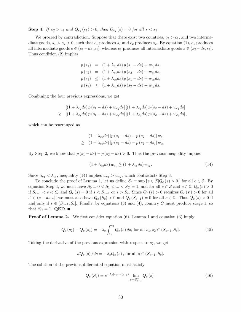
Step 4: If c2 > c1 and Qc1 (s1) > 0, then Qc2 (s) = 0 for all s < s1.

We proceed by contradiction. Suppose that there exist two countries, c2 > c1, and two interme-diate goods, s1 > s2 > 0, such that c1 produces s1 and c2 produces s2. By equation (1), c1 producesall intermediate goods s 2 (s1�ds; s1], whereas c2 produces all intermediate goods s 2 (s2�ds; s2].Thus condition (2) implies

p (s1) = (1 + �c1ds) p (s1 � ds) + wc1ds,p (s2) = (1 + �c2ds) p (s2 � ds) + wc2ds,p (s1) � (1 + �c2ds) p (s1 � ds) + wc2ds,p (s2) � (1 + �c1ds) p (s2 � ds) + wc1ds.

Combining the four previous expressions, we get

[(1 + �c2ds) p (s1 � ds) + wc2ds] [(1 + �c1ds) p (s2 � ds) + wc1ds]� [(1 + �c1ds) p (s1 � ds) + wc1ds] [(1 + �c2ds) p (s2 � ds) + wc2ds] ,

which can be rearranged as

(1 + �c2ds) [p (s1 � ds)� p (s2 � ds)]wc1� (1 + �c1ds) [p (s1 � ds)� p (s2 � ds)]wc2

By Step 2, we know that p (s1 � ds)� p (s2 � ds) > 0. Thus the previous inequality implies

(1 + �c2ds)wc1 � (1 + �c1ds)wc2 . (14)

Since �c2 < �c1 , inequality (14) implies wc1 > wc2 , which contradicts Step 3.To conclude the proof of Lemma 1, let us de�ne Sc � sup fs 2 SjQc (s) > 0g for all c 2 C. By

equation Step 4, we must have S0 � 0 < S1 < ::: < SC = 1, and for all s 2 S and c 2 C, Qc (s) > 0if Sc�1 < s < Sc and Qc (s) = 0 if s < Sc�1 or s > Sc. Since Qc (s) > 0 requires Qc (s0) > 0 for alls0 2 (s � ds; s], we must also have Qc (Sc) > 0 and Qc (Sc�1) = 0 for all c 2 C. Thus Qc (s) > 0 ifand only if s 2 (Sc�1; Sc]. Finally, by equations (3) and (4), country C must produce stage 1, sothat SC = 1. QED.

Proof of Lemma 2. We �rst consider equation (6). Lemma 1 and equation (3) imply

Qc (s2)�Qc (s1) = ��cZ s2

s1

Qc (s) ds, for all s1; s2 2 (Sc�1; Sc]. (15)

Taking the derivative of the previous expression with respect to s2, we get

dQc (s) =ds = ��cQc (s) , for all s 2 (Sc�1; Sc].

The solution of the previous di¤erential equation must satisfy

Qc (Sc) = e��c(Sc�Sc�1) lim

s!S+c�1Qc (s) . (16)

30

Lemma 1 and equation (3) also imply

Qc (Sc�1 + ds)�Qc�1 (Sc�1 � ds) = �"�c lim

s!S+c�1Qc (s) + �c�1Qc�1 (Sc�1 � ds)

#ds.

Taking the limit of the previous expression as ds goes to zero, we get

lims!S+c�1

Qc (s) = lims!S�c�1

Qc�1 (s) = Qc�1 (Sc�1) . (17)

Equation (6) derives from equations (16) and (17) and the de�nition of Qc � Qc (Sc).Let us now turn to equation (5). By Lemma 1 and equation (4), we know thatZ Sc

Sc�1

Qc (s) ds = Lc, for all c 2 C. (18)

By equations (15) and (17), we also know thatZ Sc

Sc�1

Qc (s) ds =1

�c[Qc�1 (Sc�1)�Qc (Sc)] . (19)

Equations (18) and (19) imply

Lc =1

�c[Qc�1 (Sc�1)�Qc (Sc)] , for all c 2 C. (20)

Equation (5) derives from equations (6) and (20) and the de�nition of Qc � Qc (Sc). The boundaryconditions S0 = 0 and SC = 1 have already been established in the proof of Lemma 1. QED.

Proof of Lemma 3. We �rst consider equation (7). Lemma 1 and condition (2) imply

p (Sc + ds)� (1 + �c+1ds) p (Sc)� wc+1ds � p (Sc + ds)� (1 + �cds) p (Sc)� wcds,p (Sc)� (1 + �cds) p (Sc � ds)� wcds � p (Sc)� (1 + �c+1ds) p (Sc � ds)� wc+1ds.

After simpli�cations, the two previous inequalities can be rearranged as

(�c � �c+1) p (Sc) � wc+1 � wc � (�c � �c+1) p (Sc � ds) .

Since p is continuous, taking the limit of the above chain of inequalities as ds goes to zero we get

wc+1 � wc = (�c � �c+1) p (Sc) , for all s 2 (Sc�1; Sc].

which is equivalent to equation (7) by the de�nition of pc � p (Sc).Let us now turn to equation (8). Lemma 1 and condition (2) imply

p (s+ ds) = (1 + �cds) p (s) + wcds

31

Taking the limit of the previous expression as ds goes to zero, we get

dp (s) =ds = �cp (s) + wc, for all s 2 (Sc�1; Sc].

The solution of the previous di¤erential equation must satisfy

p (Sc) = e�c(Sc�Sc�1) lim

s!S+c�1p (Sc�1) +

"e�c(Sc�Sc�1) � 1

�c

#(wc=�c) ,

which is equivalent to equation (8) by the continuity of p (�) and the de�nitions of Nc � Sc � Sc�1and pc � p (Sc). The boundary conditions derive from the fact that p0 = p (S0) = p(0) = 0 andpC = p (SC) = p (1) = 1. QED.

Proof of Proposition 1. We proceed in four steps.

Step 1: (S0; :::; SC) and (Q0; :::; QC) satisfy equations (5) and (6) if and only if

Sc = S0 +Pcc0=1

�1

�c0

�ln

"Q0 �

Pc0�1c00=1 �c00Lc00

Q0 �Pc0c00=1 �c00Lc00

#, for all c 2 C, (21)

Qc = Q0 �Pcc0=1 �c0Lc0, for all c 2 C. (22)

Let us �rst show that if (S0; :::; SC) and (Q0; :::; QC) satisfy equations (5) and (6), then they satisfyequations (21) and (22). Consider equation (22). Equations (5) and (6) imply

Qc = Qc�1 � �cLc, for all c 2 C,

By iteration we therefore have

Qc = Q0 �Pcc0=1 �c0Lc0 , for all c 2 C.

Now consider equation (21). Starting from equation (5) and iterating we get

Sc = S0 �Pcc0=1

�1

�c0

�ln

�1� �c

0Lc0

Qc0�1

�, for all c 2 C.

Equation (21) directly derives from the previous expression and equation (22). It is a matter ofsimple algebra to check that if (S0; :::; SC) and (Q0; :::; QC) satisfy equations (21) and (22), thenthey satisfy equations (5) and (6).

Step 2: There exists a unique pair of vectors (S0; :::; SC) and (Q0; :::; QC) satisfying equations(5) and (6) and the boundary conditions: S0 = 0 and SC = 1.

Let Q0�PCc=1 �cLc. By Step 1, if Q0 � Q

0, then there does not exist a pair of vec-

tors (S0; :::; SC) and (Q0; :::; QC) that satisfy equations (5) and (6). Otherwise (Q0; :::; QC) and(S0; :::; SC) would also satisfy equations (21) and (22), which cannot be the case if Q0 � Q0. Nowconsider Q0 > Q

0. From equation (21), it is easy to check that @SC=@Q0 < 0 for all Q0 > Q

0;

limQ0!Q+0SC = +1; and limQ0!+1 SC = S0. Thus conditional on having set S0 = 0, there ex-

ists a unique Q0 > Q0 such that (S0; :::; SC) and (Q0; :::; QC) satisfy equations (21) and (22) andSC = S. Step 2 derives from Step 1 and the previous observation.

32

Step 3: For any (N1; :::; NC), there exists a unique pair of vectors (w1; :::; wC) and (p0; :::; pC)satisfying equations (7) and (8) and the boundary conditions: p0 = 0 and pC = 1.

For any (N1; :::; NC), w1, and p0, there trivially exists a unique pair of vectors (w2; :::; wC) and(p1; :::; pC) that satisfy equations (7) and (8). Thus taking (N1; :::; NC) as given and having setp0 = 0, we only need to check that there exists a unique w1 such that pC = 1. To do so, we �rstestablish that pC is strictly increasing in w1. We proceed by iteration. By equation (8), we knowthat p1 is strictly increasing in w1. Thus by equation (7), w2 must be strictly increasing in w1 aswell. Now suppose that pc�1 and wc are strictly increasing in w1 for c < C. Then pc must be strictlyincreasing in w1, by equation (8), wc+1 must be strictly increasing in w1, by equation (7). At thispoint we have established, by iteration, that pC�1 and wC are strictly increasing in w1. Combiningthis observation with equation (8), we obtain that pC is strictly increasing in w1. To conclude, letus note that, by equations (7) and (8), we also have limw1!0 pC = 0 and limw1!+1 pC = +1.Since pC is strictly increasing in w1, there therefore exists a unique w1 such that pC = 1.

Steps 1-3 imply the existence and uniqueness of (S0; :::; SC), (Q0; :::; QC), (w1; :::; wC), and(p0; :::; pC) that satisfy equations (5)-(8) with boundary conditions S0 = 0, SC = 1, p0 = 0, andpC = 1. Now consider the following output levels and intermediate good prices

Qc (s) = e��c(s�Sc�1)Qc�1, for all s 2 (Sc�1; Sc],

p (s) = e�c(s�Sc�1)pc�1 +he�c(s�Sc�1) � 1

i(wc=�c) for all s 2 (Sc�1; Sc].

By construction, [Q1 (�) ; :::; QC (�)], (w1; :::; wC), and p (�) satisfy conditions (2)-(4). Thus a freetrade equilibrium exists. Since (S0; :::; SC), (Q0; :::; QC), (w1; :::; wC), and (p0; :::; pC) are unique,the free trade equilibrium is unique as well by Lemmas 1-3. QED.

B Proofs (II): Global Technological ChangeProof of Proposition 2. We decompose the proof of Proposition 2 into three parts. First, weshow that an increase in S increases the measure of stages Nc performed in all countries. Second,we show that an increase in S leads all countries to move up the supply chain. Third, we show thatan increase in S increase inequality between countries around the world.

Part I: If S0 > S, then N 0c > Nc for all c 2 C.

We �rst show that N 01 > N1 by contradiction. Suppose that N 0

1 � N1. By equation (5),equation (6) and the de�nition of Nc � Sc � Sc�1, we know that

Nc = ��1

�c

�ln

�1�

��cLc

�c�1Lc�1

��e�c�1Nc�1 � 1

��, for all c > 1, (23)

According to equation (23), we have @Nc=@Nc�1 > 0. Thus by iteration, N 01 � N1 implies N 0

c � Ncfor all countries c 2 C. This further implies

PCc=1N

0c = S0C � S00 � SC � S0 =

PCc=1Nc, which

contradicts S0C � S00 > SC � S0 by Lemma 2. Starting from N 01 > N1, we can then use equation

(23) again to show by iteration that N 0c > Nc for all c 2 C. This completes the proof of Part I.

Part II: If S0 > S, then S0c > Sc for all c 2 C.We proceed by iteration. By Lemma 2 and Part I, we know that S01 = N

01 > S1 = N1. Thus

S0c > Sc is satis�ed for c = 1. Let us now show that if S0c > Sc for 1 � c < C, then S0c+1 > Sc+1. By

33

de�nition, we know that S0c+1 = S0c + N

0c+1 and Sc+1 = Sc + Nc+1. By Part I, we also know that

N 0c+1 > Nc+1. Thus S

0c > Sc implies S

0c+1 > Sc+1. This concludes the proof of Part II.

Part III: If S0 > S, then (wc+1=wc)0 > (wc+1=wc) for all c < C.

The proof of Part III proceeds in two steps.

Step 1: If N 01 > N1, then (w2=w1)

0 > (w2=w1).

Since p0 = 0, we know from equations (7) and (8) that

w2w1

= 1 +1

�1(�1 � �2)

�e�1N1 � 1

�. (24)

Combining equation (24) and N 01 > N1, we obtain (w2=w1)

0 > (w2=w1). This completes the proofof Step 1.

Step 2: For any country 1 < c < C, if N 0c > Nc and (wc=wc�1)

0 > (wc=wc�1), then (wc+1=wc)0 >

(wc+1=wc).

Consider a country 1 < c < C. Equations (7) and (8) imply

wc+1wc

= 1 + (�c � �c+1)��e�cNc � 1

�c

�+ e�cNc

�wc�1wc

��pc�1wc�1

��(25)

By equation (7), we also know that

wcwc�1

= 1 + (�c�1 � �c)�pc�1wc�1

�, (26)

which further implies �wc�1wc

��pc�1wc�1

�=

(pc�1=wc�1)

1 + (�c�1 � �c) (pc�1=wc�1). (27)

Since (wc=wc�1)0 > (wc=wc�1) and �c�1 > �c, equation (26) immediately implies�

pc�1wc�1

�0>

�pc�1wc�1

�.

Combining this observation with equation (27)� the right-hand side of which is increasing in(pc�1=wc�1)� we obtain �

wc�1wc

�0� pc�1wc�1

�0>

�wc�1wc

��pc�1wc�1

�. (28)

To conclude, note that N 0c > Nc implies e�cN

0c > e�cNc . Thus equation (25) and inequality (28)

imply (wc+1=wc)0 > (wc+1=wc). This completes the proof of Step 2. Combining Part I with Steps

1 and 2, it is then easy to establish Part III by iteration. QED.

Proof of Proposition 3. We decompose the proof of Proposition 3 into three parts. First, weshow that a decrease in � increases the measure of stages Nc performed by all countries c < c1 anddecreases the measure of stages Nc performed by all countries c � c1, with 1 < c1 � C. Second,

34

we show that a decrease in � leads all countries to move up. Third, we show that a decrease in �decreases inequality between countries around the world.

Part I: If �0 < �, then there exists 1 < c1 � C such that N 0c > Nc if and only if c < c1.

Equation (5), equation (6), and the de�nition of Nc imply

Nc = ��1

��c

�ln

�1�

��cLc

�c�1Lc�1

��e��c�1Nc�1 � 1

��, for all c > 1, (29)

where @Nc=@Nc�1 > 0 and @Nc=@� > 0. Since �0 < �, equation (29) implies that if N 0c�1 � Nc�1

for c > 1, then N 0c < Nc. This further implies the existence of 1 � c1 � C + 1 such that

N 0c > Nc if and only if c < c1. To conclude the proof of Part I, note that if c1 = 1, thenPCc=1N

0c = S0C � S00 < SC � S0 =

PCc=1Nc, which contradicts S

0C � S00 = SC � S0 by Lemma 2.

Similarly, if c1 = C + 1, thenPCc=1N

0c = S

0C � S00 > SC � S0 =

PCc=1Nc, which also contradicts

S0C � S00 = SC � S0 by Lemma 2. This completes the proof of Part I.

Part II: If �0 < �, then S0c � Sc for all c 2 C.

We �rst show by iteration that S0c > Sc if c < c1. By Lemma 2 and Part I, we know thatS01 = N 0

1 > S1 = N1. Thus S0c > Sc is satis�ed for c = 1. Let us now show that if S0c > Scfor 1 � c < c1 � 1, then S0c+1 > Sc+1. By de�nition, we know that S0c+1 = S0c + N

0c+1 and

Sc+1 = Sc + Nc+1. By Part I, we also know that N 0c+1 > Nc+1 if c < c1 � 1. Thus S0c > Sc for

1 � c < c1 � 1 implies S0c+1 > Sc+1. This establishes that S0c > Sc if c < c1. To conclude theproof of Part II, we now show by iteration that S0c � Sc if c � c1. By Lemma 2, we know thatS0C = SC = S. Thus S

0c � Sc is satis�ed for c = C. Let us now show that if S0c � Sc for c1 < c � C,

then S0c�1 � Sc�1. By de�nition, we know that S0c�1 = S0c � N 0c and Sc�1 = Sc � Nc. By Part I,

we also know that N 0c � Nc if c > c1. This establishes that S0c � Sc if c � c1, which completes the

proof of Part II.

Part III: If �0 < �, then (wc+1=wc)0 < (wc+1=wc) for all c < C.

Throughout this part of the proof, we let eNc � �Nc and epc � �pc. The proof of Part IIIproceeds in two steps.

Step 1: If �0 < �, then eN 0c <

eNc for all countries c 2 C.The proof is similar to Part I of the proof of Proposition 2. We �rst show that eN 0

1 <eN1 by

contradiction. Suppose that eN 01 � eN1. By equation (5), equation (6) and the de�nition of eNc, we

know that eNc = �� 1�c

�ln

�1�

��cLc

�c�1Lc�1

��e�c�1

eNc�1 � 1�� , for all c > 1, (30)

where @ eNc=@ eNc�1 > 0. Thus by iteration, eN 01 � eN1 implies N 0

c � Nc for all countries c 2 C. Thisimplies �0

�PCc=1N

0c

�=PCc=1

eN 0c �

PCc=1

eNc = ��PC

c=1Nc

�. Since �0 < �, this further impliesPC

c=1N0c = S0C � S00 > SC � S0 =

PCc=1Nc, which contradicts S

0C � S00 = SC � S0 by Lemma 2.

Starting from eN 01 <

eN1, we can now use equation (30) to show by iteration that eN 0c <

eNc for allc 2 C. This completes the proof of Step 1.

Step 2: If eN 0c <

eNc for all countries c 2 C, then (wc+1=wc)0 < (wc+1=wc) for all c < C.

35

Equations (7) and (8) can be rearranged as

wc+1 = wc + (�c � �c+1) epc, for all c < C, (31)epc = e�ceNcepc�1 + �e�c eNc � 1� (wc=�c) , for all c 2 C. (32)

Following the exact same strategy as in Part III of the proof of Proposition 2, it is then easy toshow by iteration that (wc+1=wc)

0 < (wc+1=wc) for all c < C. Part II directly follows from Steps 1and 2. QED.

C Proofs (III): Local Technological ChangeProof of Proposition 4. We decompose the proof of Proposition 4 into three parts. First, weshow that an increase in Lc0 increases the measure of stages performed in country c0 and decreasesthe measure of stages performed in any other country. Second, we show that an increase in Lc0 leadsall countries all countries c < c0 to move down and all countries c > c0 move up. Third, we showthat an increase in Lc0 decreases inequality among countries c 2 f1; :::; c0g, increases inequalityamong countries c 2 fc0; :::; c1g, and decreases inequality among countries c 2 fc1; :::; Cg, withc1 2 fc0 + 1; :::; Cg.

Part I: If L0c0 > Lc0, then N0c0 > Nc0 and N

0c < Nc for all c 6= c0.

Like in our previous proofs, we will repeatedly use the following relationship

Nc = ��1

�c

�ln

�1�

��cLc

�c�1Lc�1

��e�c�1Nc�1 � 1

��, for all c > 1, (23)

where @Nc=@Nc�1 > 0 and @Nc=@Lc > 0. The proof of Part I proceeds in two steps.

Step 1: If L0c0 > Lc0, then N0c < Nc for all c > c0.

Let us �rst establish that Q0C > QC . By Lemma 1, we know that Q0C � Q0C (1) =

PCc=1Q

0c (1).

By the First Welfare Theorem, we also know that the allocation in a free trade equilibrium is Paretooptimal. Thus Q0C must be the maximum output level of the �nal good attainable given the newresource and technological constraints, i.e.,

Q0C = argmaxeQ1(�);:::; eQC(�)PCc=1

eQc (1) ,subject to PC

c=1eQc (s2)�PC

c=1eQc (s1) � �

R s2s1

PCc=1 �c

eQc (s) ds, for all s1 � s2, (33)Z S

0

eQc (s) ds � L0c, for all c 2 C, (34)

where L0c0 > Lc0 and L0c = Lc for all c 6= c0. Now consider eQ1 (�) ; :::; eQC (�) such that

eQc0 (s) � Qc0 (s) + � �c0e��c0s1� e��c0S

��L0c0 � Lc0

�, for all s 2 S,

36

and eQc (s) � Qc (s) , for all s 2 S and c 6= c0.Since Q1 (�) ; :::; QC (�) satis�es the initial resource and technological constraints, as described byconditions (3) and (4), eQ1 (�) ; :::; eQC (�) must satisfy, by construction, the new resource and tech-nological constraints, as described by conditions (33) and (34). Since L0c0 > Lc0 , we must alsohave eQc0(1) + eQC (1) = � �c0e��c0S

1� e��c0S

��L0c0 � Lc0

�+QC > QC .

Since Q0C � eQc0 (1) + eQC (1), the previous inequality implies Q0C > QC . By equation (5), equation(6), and the de�nition of Nc, we also know that

NC =

�1

�c

�ln

�1 +

�CLCQC

�.

Thus if C > c0, Q0C > QC and L0C = LC imply N

0C < NC . To conclude the proof of Step 1, note

that if N 0c < Nc for c > c0 + 1, then L

0c�1 = Lc�1 and equation (23) imply N

0c�1 < Nc�1. Thus by

iteration, N 0c < Nc for all c > c0.

Step 2: If L0c0 > Lc0, then N0c < Nc for all c < c0.

We �rst show by contradiction that if L0c0 > Lc0 and c0 > 1, then N 01 < N1. Suppose that

N 01 � N1. Since L0c = Lc for all c < c0, we can use equation (23)� the fact that @Nc=@Nc�1 > 0� to

establish by iteration that N 0c � Nc for all c < c0. Since L0c0 > Lc0 and L

0c0�1 = Lc0�1, we can

further use equation (23)� the facts that @Nc=@Nc�1 > 0 and that @Nc=@Lc > 0� to establish thatN 0c0 > Nc0 . To show that N

0c0+1

> Nc0+1, we use the two following relationships

Qc�1 =�cLc

1� e��cNc , for all c 2 C (35)

Qc =�cLce

��cNc

1� e��cNc , for all c 2 C. (36)

Equation (35) derives from equation (5) and the de�nition of Nc � Sc�Sc�1. Equation (36) furtheruses equation (6). Since N 0

c0�1 > Nc0�1 and L0c0�1 = Lc0�1, equation (36)� in particular, the fact

that @Qc=@Nc < 0� implies Q0c0�1 < Qc0�1. Since Q0c0�1 < Qc0�1 and N

0c0 > Nc0 , equation (6)

implies Q0c0 < Qc0 . Finally, since Q0c0 < Qc0 and L

0c0+1

= Lc0+1, equation (35)� in particular, thefact that @Qc�1=@Nc < 0� implies N 0

c0+1> Nc0+1. Since N

0c0+1

> Nc0+1, and L0c = Lc for all

c > c0, we can further use equation (23)� in particular, the fact that @Nc=@Nc�1 > 0� to establishby iteration that N 0

c > Nc for all c > c0. This impliesPCc=1N

0c = S

0C � S00 > SC � S0 =

PCc=1Nc,

which contradicts S0C � S00 = SC � S0 = 1 by Lemma 2. At this point, we have established that ifL0c0 > Lc0 and c0 > 1, then N

01 < N1. To conclude the proof of Step 2, note that if N

0c < Nc for

c < c0 � 1, then L0c+1 = Lc+1 and equation (23) imply N 0c+1 < Nc+1. Thus by iteration, N

0c < Nc

for all c < c0. Part I directly derives from Step 1, Step 2, and the fact thatPCc=1N

0c =

PCc=1Nc

= 1, by Lemma 2.

Part II: If L0c0 > Lc0, then S0c � Sc for all c < c0 and S0c � Sc for all c � c0.

The proof of Part II proceeds in two steps.

Step 1: If L0c0 > Lc0, then S0c � Sc for all c � c0.

37

We proceed by iteration. By Lemma 2, we know that S0C = SC = S. Thus S0c � Sc is satis�ed

for c = C. Let us now show that if S0c � Sc and c > c0, then S0c�1 � Sc�1. Since c > c0,L0c0 > Lc0 and Part I imply N

0c < Nc. Combining this observation with S

0c � Sc and the de�nition

of Nc � Sc � Sc�1, we obtain S0c�1 � Sc�1. This completes the proof of Step 1.

Step 2: If L0c0 > Lc0, then S0c�1 � Sc�1 for all c � c0.

We proceed by iteration. By Lemma 2, we know that S00 = S0 = 0. Thus S0c�1 � Sc�1 issatis�ed for c = 1. Let us now show that if S0c�1 � Sc�1 and c < c0, then S0c � Sc. Since c < c0,L0c0 > Lc0 and Part I imply N

0c < Nc. Combining this observation with S0c�1 � Sc�1 and the

de�nition of Nc � Sc � Sc�1, we obtain S0c � Sc. This completes the proof of Step 2. Part IIdirectly follows from Steps 1 and 2

Part III: If L0c0 > Lc0, then there exists c0 + 1 � c1 � C such that (wc+1=wc)0 � wc+1=wc for

all 1 � c < c0; (wc+1=wc)0 � wc+1=wc for all c0 � c < c1; and (wc+1=wc)

0 � wc+1=wc for allc1 � c < C.

The proof of Part III proceeds in three steps.

Step 1: If L0c0 > Lc0, then (wc+1=wc)0 < (wc+1=wc) for all c < c0.

By Part I, we know that N 0c < Nc for all c < c0. Thus we can use the same argument as in Part

III of the proof of Proposition 2 to show that (wc+1=wc)0 < (wc+1=wc) for all c < c0.

Step 2: If L0c0 > Lc0, then there exists c0 � c1 � C such that (wc+1=wc)0 � wc+1=wc for all

c0 � c < c1 and (wc+1=wc)0 � wc+1=wc for all c1 � c < C.

By Part I, we also know that N 0c > Nc for all c > c0. Thus we can again use the same

argument as in Part III of the proof of Proposition 2 to show that if there exists ec � c0 such that(wec+1=wec)0 < (wec+1=wec), then (wc+1=wc)0 < (wc+1=wc) for all ec � c < C. To conclude the proofof Step 2, let us just de�ne c1 � inf

�c � c0j (wc+1=wc)0 < (wc+1=wc)

. By construction, wc+1=wc

rises for all c0 � c < c1 and falls for all c1 � c < C. In order to complete the proof of Part III, theonly thing left to show is that c1 > c0, which is what we establish in our �nal step.

Step 3: If L0c0 > Lc0 and c0 6= C, then (wc0+1=wc0)0 > (wc0+1=wc0).

We proceed by contradiction. Suppose that (wc0+1=wc0)0 � (wc0+1=wc0). Then for any " > 0,

there must also exist Lc0 � ~Lc0 <~L0c0 � L

0c0 such that j~L

0c0 � ~Lc0 j < " and

( ~wc0+1= ~wc0)0 � ( ~wc0+1= ~wc0) , (37)

where ( ~w1; :::; ~wC) and ( ~w01; :::; ~w0C) denote the world income distribution if labor endowments in

country c0 are equal to eLc0 and ~L0c0 , respectively. For j~L0c0 � ~Lc0 j small enough, Lemma 2 implies~S01 < ~S1 < ~S02 < ::: < ~S0c0�1 <

~Sc0�1 < ~Sc0 <~S0c0 <

~Sc0+1 < ::::, (38)

where�~S1; :::; ~SC

�and

�~S01; :::;

~S0C

�denote the pattern of vertical specialization if labor endowments

in country c0 are equal to eLc0 and ~L0c0 , respectively. First, note that for any c < c0 � 1, since

38

~S0c < ~Sc < ~S0c+1 <~Sc+1, condition (2) implies that

~p0�~S0c+1

�~w0c+1

=e�c+1(

~S0c+1� ~Sc)~p0�~Sc

�~w0c+1

+e�c+1(

~S0c+1� ~Sc) � 1�c+1

,

~p�~S0c+1

�~wc+1

=e�c+1(

~S0c+1� ~Sc)~p�~Sc

�~wc+1

+e�c+1(

~S0c+1� ~Sc) � 1�c+1

,

where ~p (�) and ~p0 (�) denote the schedule of prices if labor endowments in country c0 are equal toeLc0 and ~L0c0 , respectively. Since ~S0c+1 > ~Sc, the two previous equations further imply that for anyc < c0 � 1,

~p0�~Sc

�= ~w0c+1 � ~p

�~Sc

�= ~wc+1 ) ~p0

�~S0c+1

�= ~w0c+1 � ~p

�~S0c+1

�= ~wc+1. (39)

Second, note that for any c < c0, since ~Sc�1 < ~S0c < ~Sc, condition (2) also implies that

~p0�~Sc

�~w0c+1

=e�c+1(

~Sc� ~S0c)~p0�~S0c

�~w0c+1

+e�c+1(

~Sc� ~S0c) � 1�c+1

, (40)

~p�~Sc

�~wc+1

=e�c(

~Sc� ~S0c)~p�~S0c

�~wc+1

+e�c(

~Sc� ~S0c) � 1�c

�~wc~wc+1

�. (41)

Let us now show that if ~p0�~S0c

�= ~w0c � ~p

�~S0c

�= ~wc, then

e�c+1(~Sc� ~S0c)~p0

�~S0c

�~w0c+1

�e�c(

~Sc� ~S0c)~p�~S0c

�~wc+1

, (42)

e�c+1(~Sc� ~S0c) � 1�c+1

� e�c(~Sc� ~S0c) � 1�c

�~wc~wc+1

�. (43)

We start with inequality (42), which can be rearranged as

e�c+1(~Sc� ~S0c) ~w0c

~w0c+1

~p0�~S0c

�~w0c

� e�c( ~Sc� ~S0c) ~wc~wc+1

~p�~S0c

�~wc

.

By equation (7), we know that

e�c(~Sc� ~S0c) ~wc

~wc+1

~p�~S0c

�~wc

=

~p( ~S0c)~wc

1 + (�c � �c+1)~p( ~Sc)~wc

, (44)

e�c+1(~Sc� ~S0c) ~w0c

~w0c+1

~p0�~S0c

�~w0c

=

~p0( ~S0c)~w0c

1 + (�c � �c+1)~p0( ~S0c)~w0c

. (45)

39

Under the assumption that ~p0�~S0c

�= ~w0c � ~p

�~S0c

�= ~wc, equations (44) and (45) imply

e�c+1(~Sc� ~S0c) ~w0c

~w0c+1

~p0�~S0c

�~w0c

�~p( ~S0c)~wc

1 + (�c � �c+1)~p( ~S0c)~wc

> e�c(~Sc� ~S0c) ~wc

~wc+1

~p�~S0c

�~wc

,

where the second inequality also uses the fact that ~S0c < ~Sc. Thus inequality (42) holds. Let usnow consider inequality (43), which can be rearranged as

�c

�e�c+1(

~Sc� ~S0c) � 1�

�c+1

�e�c(

~Sc� ~S0c) � 1� � ~wc

~wc+1. (46)

Since ~Sc�1 < ~S0c for any c < c0, condition (2) implies ~pc�~Sc

�= ~wc �

he�c(

~Sc� ~Sc�1) � 1i=�c >h

e�c(~Sc� ~S0c) � 1

i=�c. Combining the previous inequality with equation (7), we obtain

~wc~wc+1

=1

1 + (�c � �c+1)~p( ~Sc)~wc

<�c

�c + (�c � �c+1)he�c(

~Sc� ~S0c) � 1i (47)

By inequalities (46) and (47), a su¢ cient condition for inequality (43) to hold is

�c

he�c+1(

~Sc� ~S0c) � 1i

�c+1

he�c(

~Sc� ~S0c) � 1i � �c

�c + (�c � �c+1)he�c(

~Sc� ~S0c) � 1i ,

which can be rearranged as �c=h1� e��c( ~Sc� ~S0c)

i� �c+1=

h1� e��c+1( ~Sc� ~S0c)

i. The previous in-

equality necessarily holds since f(x) � x1�e�tx is increasing in x for t > 0. At this point, we

have established that inequalities (42) and (43) hold if ~p0�~S0c

�= ~w0c � ~p

�~S0c

�= ~wc. Combining this

observation with equations (40) and (41), we further have that for any c < c0,

~p0�~S0c

�= ~w0c � ~p

�~S0c

�= ~wc ) ~p0

�~Sc

�= ~w0c+1 � ~p

�~Sc

�= ~wc+1. (48)

Since ~p0 (0) = ~p (0) = 0, we know that ~p0�~S0

�= ~w01 � ~p

�~S0

�= ~w1. Thus we can use implications

(39) and (48) to establish, by iteration, that

~p0�~Sc0�1

�~w0c0

�~p�~Sc0�1

�~wc0

. (49)

40

Since eSc0 < eS0c0 , we know from condition (2) that

~p0�~Sc0

�~w0c0

=e�c0(

~Sc0� ~Sc0�1)~p0�~Sc0�1

�~w0c0

+e�c0(

~Sc0� ~Sc0�1) � 1�c0

, (50)

~p�~Sc0

�~wc0

=e�c0(

~Sc0� ~Sc0�1)~p�~Sc0�1

�~wc0

+e�c0(

~Sc0� ~Sc0�1) � 1�c0

: (51)

Inequality (49) and equations (50) and (51) imply ~p0�~Sc0

�= ~w0c0 � ~p

�~Sc0

�= ~wc0 . Finally, sinceeSc0 < eS0c0 , we also know that ~p0

�~S0c0

�= ~w0c0 > ~p0

�~Sc0

�= ~w0c0 . Combining these two observations,

we get ~p0�~S0c0

�= ~w0c0 > ~p

�~Sc0

�= ~wc0 . Together with equation (7), the previous inequality implies

( ~wc0+1= ~wc0)0 > ( ~wc0+1= ~wc0), which contradicts inequality (37). Thus (wc0+1=wc0)

0 > (wc0+1=wc0),which implies c1 � inf

�c � c0j (wc+1=wc)0 < (wc+1=wc)

> c0. As mentioned above, Part III

directly follows from Steps 1-3. QED.

Proof of Proposition 5. We decompose the proof of Proposition 5 into three parts. First, weshow that a decrease in �c0 increases the measure of stages Nc performed in all countries c < c0and decreases the measure of stages Nc performed in all countries c > c0. Second, we show thata decrease in �c0 leads all countries to move up. Third, we show that a decrease in �c0 increasesinequality among countries c 2 f1; :::; c0g, decreases inequality among countries c 2 fc0; c0 + 1g,increases inequality among countries c 2 fc0 + 1; :::; c1g, and decreases inequality among countriesc 2 fc1; :::; Cg, with c1 2 fc0 + 1; :::; Cg.

Part I: If �0c0 < �c0, then N0c > Nc for all c < c0 and N

0c < Nc for all c > c0.

Like in our previous proofs, we will repeatedly use the following relationship

Nc = ��1

�c

�ln

�1�

��cLc

�c�1Lc�1

��e�c�1Nc�1 � 1

��, for all c > 1, (23)

where @Nc=@Nc�1 > 0, @Nc=@�c�1 > 0, and @Nc=@�c > 0. The proof of Part I proceeds in twosteps.

Step 1: If �0c0 < �c0, then N0c < Nc for all c > c0.

Let us �rst establish that Q0C > QC . By the same argument as in Step 1 of Proposition 4, Q0C

must be such thatQ0C = argmaxeQ1(�);:::; eQC(�)

PCc=1

eQc (S) ,subject to PC

c=1eQc (s2)�PC

c=1eQc (s1) � �

R s2s1

PCc=1 �

0ceQc (s) ds, for all s1 � s2, (52)Z S

0

eQc (s) ds � Lc, for all c 2 C, (53)

41

where �0c0 < �c0 and �0c = �c for all c 6= c0. Now consider eQ1 (�) ; :::; eQC (�) such that

eQc0 (s) � e�(�c0��0c0)(Sc0�s)Qc0 (s)+

�0c0e

��0c0s

1� e��0c0S

!Z Sc0

Sc0�1

h1� e�(�c0��

0c0)(Sc0�t)

iQc0 (t) dt, for all s 2 S,

and eQc (s) � Qc (s) , for all s 2 S and c 6= c0.Since Q1 (�) ; :::; QC (�) satisfy the initial resource and technological constraints, as described byequations (3) and (4), eQ1 (�) ; :::; eQC (�) must satisfy, by construction, the new resource and tech-nological constraints, as described by equations (52) and (53). Since �0c0 < �c0 , we must alsohave

eQc0 (1) + eQC (1) = � �c0e��c0S1� e��c0S

�Z Sc0

Sc0�1

h1� e�(�c0��

0c0)(Sc0�t)

iQc0 (t) dt+QC > QC .

Since Q0C � eQc0 (1)+ eQC (1), the previous inequality implies Q0C > QC . Combining this observationwith equation (36) and the fact that c0 6= C, which implies �0C = �C , we get N 0

C < NC . To concludethe proof of Step 1, note that if N 0

c < Nc for c > c0 + 1, then �0c�1 = �c�1 and equation (23)� the

fact that @Nc=@Nc�1 > 0� imply N 0c�1 < Nc�1. Thus by iteration, N

0c < Nc for all c > c0.

Step 2: If �0c0 < �c0, then N0c > Nc for all c < c0.

We �rst show by contradiction that if �0c0 < �c0 and c0 > 1, then N 01 > N1. Suppose that

N 01 � N1. Since �0c = �c for all c < c0, we can use equation (23)� the fact that @Nc=@Nc�1 > 0

� to establish by iteration that N 0c � Nc for all c < c0. Since �0c0 < �c0 , �

0c0�1 = �c0�1, and

N 0c0�1 � Nc0�1, we can use equation (23)� the facts that @Nc=@Nc�1 > 0 and @Nc=@�c > 0� to

establish that N 0c0 < Nc0 . By Step 1, we also know that N 0

c < Nc for all c > c0. This impliesPCc=1N

0c = S

0C � S00 < SC � S0 =

PCc=1Nc, which contradicts S

0C � S00 = SC � S0 = 1 by Lemma

2. At this point, we have established that if �0c0 < �c0 and c0 > 1, then N01 > N1. To conclude the

proof of Step 2, note that if N 0c > Nc for c < c0 � 1, then �0c = �c, �0c+1 = �c+1, and equation (23)

imply N 0c+1 > Nc+1. Thus by iteration, N

0c > Nc for all c < c0. Part I directly derives from Steps

1 and 2.

Part II: If �0c0 < �c0, then S0c � Sc for all c 2 C.

The proof of Part II proceeds in two steps.

Step 1: If �0c0 < �c0, then S0c � Sc for all c � c0.

The proof is identical to the proof of Step 1 Part II of Proposition 4 and omitted.

Step 2: If �0c0 < �c0, then S0c�1 � Sc�1 for all c � c0.

We proceed by iteration. By Lemma 2, we know that S00 = S0 = 0. Thus S0c�1 � Sc�1 issatis�ed for c = 1. Let us now show that if S0c�1 � Sc�1 and c < c0, then S0c � Sc. Since c < c0,�0c0 < �c0 and Part I imply N

0c > Nc. Combining this observation with S0c�1 � Sc�1 and the

de�nition of Nc � Sc � Sc�1, we obtain S0c � Sc. This completes the proof of Step 2. Part IIdirectly derives from Steps 1 and 2.

42

Part III: If �0c0 < �c0, then there exist c0 < c1 � C such that (wc+1=wc)0 � wc+1=wc for all c < c0;

(wc0+1=wc0)0 � wc0+1=wc0 ; (wc+1=wc)

0 � wc+1=wc for all c0 < c < c1; and (wc+1=wc)0 � wc+1=wcfor all c1 � c < C.

The proof of Part III proceeds in four steps.

Step 1: If �0c0 < �c0, then (wc+1=wc)0 > (wc+1=wc) for all c < c0.

By Part I, we know that N 0c > Nc for all c < c0. Thus we can use the same argument as in Part

III of the proof of Proposition 2 to show that (wc+1=wc)0 > (wc+1=wc) for all c < c0.

Step 2: If �0c0 < �c0and c0 > 1, then S0c0 � S

0c0�1 <

�c0�0c0(Sc0 � S0c0�1).

In the proof of Step 2, we let Q0(s) and p0 (s), denote the output at stage s and the price ofstage s if the failure rate in country c0 is equal to �0c0 .From Equation (36), we have

Q1 =�1L1e

��1N1

1� e��1N1 .

Similarly, we have

Q0(S1) =�1L

11e��1N 0

1

1� e��1N 01;

where L11 is the population in county 1 employed in producing goods (0; S1) when the failure rateof country c0 is �0c0 . The two previous equations, together with N

01 > N1 and L

11 < L1, therefore,

imply Q0(S1) < Q1. Assume that Q0(Sc) < Qc holds for some 1 � c � c0 � 2. Since c+ 1 < c0,

Qc+1 = e��c+1Nc+1Qc

> e��c+1(Sc+1�S0c+S

0c�Sc)Q0(Sc)

� e��c(S0c�Sc)��c+1(Sc+1�S0c)Q0(Sc)

= e��c+1(Sc+1�S0c)Q0(S0c)

= Q0(Sc+1):

Therefore, by iteration,Q0(Sc) < Qc for all 1 � c � c0 � 1. (54)

By equation (54), which implies Q0(Sc0�1) < Qc0�1, and equation (1), we have

Q0c0 = e��0c0(S0c0�S

0c0�1

)��c0�1(S0c0�1

�Sc0�1)Q0(Sc0�1)

< e��0c0(S0c0�S

0c0�1

)��c0�1(S0c0�1

�Sc0�1)Qc0�1. (55)

Equation (6) impliesQc0 = e

��c0 (Sc0�Sc0�1)Qc0�1. (56)

By the proof of Part I of Proposition 5, we have N 0c0+1

< Nc0+1. Equation (35) and N0c0+1

< Nc0+1imply Q0c0 > Qc0 . Equation (55), equation (56), and Q

0c0 > Qc0 imply

e��0c0(S0c0�S

0c0�1

)��c0�1(S0c0�1

�Sc0�1) > e��c0 (Sc0�Sc0�1),

43

which implies

S0c0 � S0c0�1 <

�c0�0c0(Sc0 � S0c0�1)�

�c0�1 � �c0�0c0

(S0c0�1 � Sc0�1) ��c0�0c0(Sc0 � S0c0�1),

concluding the proof of Step 2.

Step 3: If �0c0 < �c0and c0 < C, then (wc0+1=wc0)0 � wc0+1=wc0.

By Part II, there exists, �, a small neighborhood of �c0 , such that if the failure rate in countryc0 is equal to �0c0 2 � and �

0c0 < �c0 , the following sequence of inequalities holds:

S1 < S01 < S2 < S

02 < ::: < Sc0�1 < S

0c0�1 < Sc0 < S

0c0 < Sc0+1 < :::;

where (S01; :::; S0C) denote the pattern of vertical specialization if the failure rate in country c0 is

equal to �0c0 . In exactly the same way as we have proceeded in Part III of Proposition 4, one canshow by iteration that

p0(S0c0�1)

w0c0�p(S0c0�1)

wc0.

Notice that the fact that failure rate in country c0 falls from �c0 to �0c0 only loosens the inequality.

Equations (9) and (2) imply

w0c0+1w0c0

� 1 = (�0c0 � �c0+1)"p0(S0c0�1)

w0c0e�

0c0(S0c0�S

0c0�1

) +e�

0c0(S0c0�S

0c0�1

) � 1�0c0

#.

From Step 2, we therefore have

w0c0+1w0c0

� 1 < (�0c0 � �c0+1)"p(S0c0�1)

wc0e�c0 (Sc0�S

0c0�1

) +e�c0 (Sc0�S

0c0�1

) � 1�0c0

#(57)

Equation (57) and �0c0 < �c0 imply

w0c0+1w0c0

� 1 < (�c0 � �c0+1)"p(S0c0�1)

wc0e�c0 (Sc0�S

0c0�1

) +e�c0 (Sc0�S

0c0�1

) � 1�c0

#. (58)

Equations (9) and (2) imply

wc0+1wc0

� 1 = (�c0 � �c0+1)"p(S0c0�1)

wc0e�c0 (Sc0�S

0c0�1

) +e�c0 (Sc0�S

0c0�1

) � 1�c0

#. (59)

Finally, equations (58) and (59) imply w0c0+1=w0c0 < wc0+1=wc0 .

Step 4: If �0c0 < �c0, then there exists c0 < c1 � C such that (wc+1=wc)0 � wc+1=wc for all

c0 < c < c1; and (wc+1=wc)0 � wc+1=wc for all c1 � c < C.

By Part I, we also know that N 0c > Nc for all c > c0. Thus we can again use the same

argument as in Part III of the proof of Proposition 2 to show that if there exists ec > c0 such that(wec+1=wec)0 < (wec+1=wec), then (wc+1=wc)0 < (wc+1=wc) for all ec � c < C. To conclude the proof

44

of Step 4, let us just de�ne c1 � inf�c > c0j (wc+1=wc)0 < (wc+1=wc)

. By construction, wc+1=wc

rises for all c0 < c < c1 and falls for all c1 � c < C. This concludes the proof of Part III. QED.

D Proofs (IV): ExtensionsProof of Lemma 4. By Lemma 1, we already know that Lemma 4 is true if � = 1. In the restof this proof we therefore assume that � < 1. We proceed in two steps.

Step 1: In any competitive equilibrium, Cu is a step-function for all u 2�0; QW

�.

We proceed by contradiction. Suppose that Cu is not a step-function. In this case, the numberof international transactions associated with the production of that particular unit must be in�nite.Thus the cost of producing that unit must be in�nite as well, which is incompatible with zero pro�ts.

Step 2: In any competitive equilibrium, Cu is increasing in s for all u 2�0; QW

�.

Let us start by computing the expected cost of producing a given unit u. By Step 1, we knowthat that there must be a sequence of countries fcu1 ; :::; cung and stages fsu1 ; :::; sung such that: (i)cuk 6= cuk+1 for all k = 1; ::; n � 1; (ii) su0 = 0 < su1 < ::: < sun�1 < sun = S; and (iii) Cu (s) = cuk forall s 2

�suk�1; s

uk

�. Let puk denote the cost of producing that unit up to stage s

uk . By the same logic

as in the proof of Lemma 3, we know that fpu1 ; :::; pung satisfy

puk = e�cukNuk puk�1 +

�e�cukNuk � 1

� �wcuk=�c

uk

�,

where Nuk � suk � suk�1. Using the previous expression and iterating, it is then easy to check that

the expected cost of producing unit u is given by

pun =nPn

k=1

hQk0>k e

�cuk0Nuk0i �e�cukNuk � 1

� �wcuk=�c

uk

�o.�n.

The rest of our proof proceeds by contradiction. Suppose that Cu is not weakly increasing. Thenthere must exist k0 2 f1; :::; n� 1g and c > c0 such that cuk0 = c and cuk0+1 = c0. Suppose, inaddition, that Nu

k0= suk0 � s

uk0�1 � s

uk0+1

� suk0 = Nuk0+1

. The other case can be treated in a similar

manner. Now consider an alternative allocation of stages to countries, eCu, in which country c0produces all stages from suk0�1 to s

uk0and c produces all stages from suk0+1�Nk0 to s

uk0+1

. The restof the allocation of stages to countries is the same as in Cu. Let epun denote the expect unit cost ofthe �nal good associated with eCu:

epun =nPk0�1

k=1

h�Qk0>k e

�cuk0Nuk0�i�

e�cukNuk � 1

� �wcuk=�c

uk

�+he�cNu

k0

�Qk0>k0+1

e�cuk0Nuk0�i�

e�c0N

uk0+1 � 1

�(wc0=�c0)

+hQ

k0>k0+1e�cuk0Nuk0i �e�cNu

k0 � 1�(wc=�c)

+Pnk>k0+1

hQk0>k e

�cuk0Nuk0i �e�cukNuk � 1

� �wcuk=�c

uk

�o.�en

where, by construction, we must have en � n. Under perfect competition, we know that unit costs

45

of production must be minimized. Thus we must have epun � pun. Since en � n, this further requireshe�cNu

k0

�Qk0>k0+1

e�cuk0Nuk0�i�

e�c0N

uk0+1 � 1

�(wc0=�c0) +

hQk0>k0+1

e�cuk0Nuk0i �e�cNu

k0 � 1�(wc=�c)

�hQ

k0>k0e�cuk0Nuk0i �e�cNu

k0 � 1�(wc=�c) +

hQk0>k0+1

e�uck0

Nuk0i �e�c0N

uk0+1 � 1

�(wc0=�c0) ,

which simpli�es into wc0 � (�c0=�c)wc > wc. But if the previous inequality holds, then startingfrom the allocation Cu, the cost of producing unit u could be strictly lowered by performing alltasks in

�suk0�1; s

uk0+1

�in country c: it reduces the rate of mistakes, it reduces wages, and it reduces

the number of international transactions. Since unit costs must be minimized in any competitiveequilibrium, we have established, by contradiction, that Cu is increasing in s for all u 2

�0; QW

�.

QED.

Proof of Lemma 5. We proceed in two steps.

Step 1: In any free trade equilibrium, if Ac < Lc, then Ac0 = 0 for all c0 > c.

We proceed by contradiction. Suppose that there exist c0 > c such that Ac0 > 0 and Ac < Lc.Since the production function for the �nal good, F , is identical across countries, zero pro�ts in the�nal good sector and Ac0 > 0 require wc � wc0 . Since �c0 < �c, the unit cost of production of anyintermediate good in any chain is then lower in country c0 than in country c, thereby contradictingAc < Lc.

Step 2: In any free trade equilibrium, there exists a sequence of stages S0 � 0 � S1 � ::: � SC = Ssuch that for all n 2 N , s 2 S, and c 2 C, Qnc (s) > 0 if and only if s 2 (Sc�1; Sc].

Using the same argument as in Lemma 1, one can easily show that for all n 2 N , there existSn0 � 0 � Sn1 � ::: � SnC = S such that for all s 2 S and c 2 C, Qnc (s) > 0 if and only ifs 2 (Snc�1; Snc ]. Let us now show that for all n; n0 2 N and c 2 C, Snc = Sn

0c . We proceed by

contradiction. Suppose, without loss of generality, that there exist n; n0; c such that Snc < Sn0c . Let

c1 � infnc 2 CjSnc < Sn

0c

o, c2 � inf

�c0 � c1jSnc0 > Snc1

, and � � min

�Sn

0c1 � S

nc ; S

nc2 � S

nc

�. By

construction, c1 produces all intermediate goods s 2 (Snc ; Snc +�] in chain n0, whereas c2 producesall intermediate goods s 2 (Snc ; Snc +�] in chain n. Thus for all � 2 (0;�], condition (2) implies

pn0(Snc + �) = e�c1�pn

0(Snc ) +

�e�c1� � 1

�(wc1=�c1) ,

pn (Snc + �) = e�c2�pn (Snc ) +�e�c2� � 1

�(wc2=�c2) ,

pn0(Snc + �) � e�c2�pn

0(Snc ) +

�e�c2� � 1

�(wc2=�c2) ,

pn (Snc + �) � e�c1�pn (Snc ) +�e�c1� � 1

�(wc1=�c1) ,

where pn (�) and pn0 (�) represent the price of intermediate goods in chains n and n0, respectively.By de�nition of c1, we know that pn (Snc ) = p

n0 (Snc ) � pc. Thus the four previous conditions imply

e�c1� (pc + wc1=�c1)� e�c2� (pc + wc2=�c2) + (wc2=�c2)� (wc1=�c1) = 0.

Since the previous equation holds for all � 2 (0;�], �c1 6= �c2 implies pc + wc1=�c1 = pc + wc2=�c2= 0, which contradicts wc1 ; wc2 > 0.

Lemma 5 follows directly from Steps 1 and 2. QED.

46

Proof of Lemma 1 with heterogeneous stages. Following the exact same strategy as in theproof of Lemma 1, one can easily show that p (�) is continuous and strictly increasing in s and thatwc is strictly increasing in c. Let us now show that if c2 > c1 and Qc1 (s1) > 0, then Qc2 (s) = 0 forall s < s1. We proceed by contradiction. Suppose that there exist two countries, c2 > c1, and twointermediate goods, s1 > s2 > 0, such that c1 produces s1 and c2 produces s2. Pro�t maximizationnow requires

p (s1) = [1 + �c1 (s1) ds] p (s1 � ds) + wc1ds,p (s2) = [1 + �c2 (s2) ds] p (s2 � ds) + wc2ds,p (s1) � [1 + �c2 (s1) ds] p (s1 � ds) + wc2ds,p (s2) � [1 + �c1 (s2) ds] p (s2 � ds) + wc1ds.

Combining the four previous expressions, we get

f[1 + �c2 (s1) ds] p (s1 � ds) + wc2dsg f[1 + �c1 (s2) ds] p (s2 � ds) + wc1dsg� f[1 + �c1 (s1) ds] p (s1 � ds) + wc1dsg f[1 + �c2 (s2) ds] p (s2 � ds) + wc2dsg ,

which can be rearranged as

[1 + �c2 (s1) ds] [p (s1 � ds)� p (s2 � ds)]wc1� [1 + �c1 (s2) ds] [p (s1 � ds)� p (s2 � ds)]wc2

+ [�c1 (s1) + �c2 (s2)� �c2 (s1)� �c1 (s2)] p (s2 � ds) p (s1 � ds)

Since �c(s) is weakly submodular in (s; c), c2 > c1 and s1 > s2 imply �c1 (s1)+�c2 (s2)��c2 (s1)��c1 (s2) � 0. Thus the previous inequality implies

[1 + �c2 (s1) ds] [p (s1 � ds)� p (s2 � ds)]wc1 (60)

� [1 + �c1 (s2) ds] [p (s1 � ds)� p (s2 � ds)]wc2

Since p (s) is strictly increasing in s, we know that p (s1 � ds) � p (s2 � ds) > 0. Thus inequality(60) further implies

[1 + �c2 (s1) ds]wc1 � [1 + �c1 (s2) ds]wc2 . (61)

Finally, since �c (s) is strictly decreasing in c and weakly increasing in s, c2 > c1 and s1 > s2imply �c2 (s1) < �c1 (s2). Inequality (61) therefore implies wc1 > wc2 , which contradicts wc strictlyincreasing in c. The rest of the proof is similar to the proof of Lemma 1 and omitted. QED.

47