1

An economic assessment of the Kyoto Protocol using the Global Trade and

Environment Model

Vivek Tulpulé, Stephen Brown, Jaekyu Lim, Cain Polidano, Hom Pant and Brian S. Fisher

The Economic Modelling of Climate Change:Background Analysis for the Kyoto Protocol

OECD WorkshopOECD Headquarters, Paris, 17–18 September 1998

Ratification of the Kyoto Protocol will have major medium and long term implications for theAustralian economy and for the international community. The protocol is one of the most ambitiousand far reaching environmental policy initiatives ever attempted.

Greenhouse gas emission abatement targets agreed to by individual countries are set out in Annex Bto the protocol. The protocol includes provisions for the use of flexibility mechanisms such as jointimplementation, the clean development mechanism and emissions trading to help Parties meet theirtarget commitments. These flexibility mechanisms allow emission abatement to take place inrelatively low cost locations, thereby reducing the overall costs associated with meeting emissiontargets. No agreement was reached in the protocol on the principles and guidelines for the operationof these schemes and further negotiations are required before they can be implemented.

In this paper ABARE’s Global Trade and Environment Model (GTEM) is used to analyse thepotential of international emissions trading as a mechanism for helping to achieve the abatementcommitments agreed to in the protocol. First, a detailed description of the key features of the modelis presented. Second, analysis showing that a system of internationally tradable emission quotaswould decrease the cost of achieving abatement commitments is presented. In addition, it is shownthat emissions trading would improve the effectiveness of the protocol because the extent of carbonleakage would be reduced. Finally, the paper examines the sensitivity of the projected carbonemission penalties required under an international emissions trading scheme to key assumptionsmade in the model.

2

IntroductionNegotiations for the Kyoto Protocol to the UN Framework Convention on Climate Change concludedon 11 December 1997. Under the protocol, parties listed in Annex B to the protocol agreed to reducetheir greenhouse gas emissions to at least 5.2 per cent below 1990 levels over a commitment periodspanning the period 2008–12 (table 1). The emission reduction targets are comprehensive in theircoverage of greenhouse gases not covered by the Montreal Protocol as well as of sources and sinksfor these gases. (A copy of the protocol can be found at http://www.unfccc.de./)

Significantly, the use of so called ‘flexibility mechanisms’ that could reduce the economic costs ofachieving emission reduction targets was agreed to in the protocol. These mechanisms include: jointimplementation (Article 6), the clean development mechanism (Article 12) and internationalemissions trading (Article 17). While the Kyoto Protocol provides a legal basis for the introduction ofsuch mechanisms, negotiations are now underway to determine the principles and guidelines thatcould govern their implementation.

At the time of writing, two distinct negotiating blocs had formed among the Annex B countries — the‘umbrella group’, consisting of Australia, Canada, Japan, Iceland, New Zealand, Norway, the RussianFederation, the Ukraine and the United States; and a group that includes most other Annex Bcountries, led by the European Union. The umbrella group has expressed support for an internationalemissions trading system with characteristics similar to those observed in markets for other financialinstruments. The European Union has been more muted in its support of emissions trading.

The purpose in this paper is to provide estimates of the global economic impacts associated withreducing carbon dioxide emissions from fossil fuel combustion. Estimates of the impacts of emissionabatement policies in this paper are based on simulation results from the Global Trade andEnvironment Model (GTEM).

An important limitation of the analysis presented here is its focus on emissions of carbon dioxidefrom fossil fuel combustion. At this point data constraints prevent adequate analysis of thecomprehensive approach to greenhouse gas reduction embodied in the Kyoto Protocol. This meansthat results in this paper are indicative only of the economic impacts that may occur when all gasesand sinks are modeled. ABARE is in the process of extending GTEM to include additionalgreenhouse gases and sinks to enable a more comprehensive assessment of the Kyoto Protocol.

Three different policy scenarios have been analysed, each based on alternative negotiating outcomesin a post-Kyoto setting.

Independent abatement: Annex B countries act independently to meet their Kyoto commitment interms of emissions of carbon dioxide from fossil fuel combustion to levels specified in table 1.

Annex B trading: Annex B countries engage in emissions trading, where initial allocations ofemissions quota are at levels specified in table 1.

Double bubble: Two emissions trading bubbles are formed, one consisting of members of theumbrella group and another consisting of the remaining Annex B countries, including the EuropeanUnion. Countries within each bubble trade in emissions quotas, but there is no quota trade betweenbubbles. Again, initial allocations of emissions quota are at levels specified in table 1.

The comparative assessment in this paper focuses on the effects of emission reduction policies onmarginal emission abatement costs, real GNP and GDP, real consumption, trade and changes inemissions in developing countries resulting from carbon leakage. Uncertainties about energy marketdevelopments in the future will also have a major influence on policy assessments. To address thisissue, the sensitivity of model results to key assumptions made regarding the energy sector isreported.

3

The Global Trade and Environment Model

GTEM is a dynamic general equilibrium model of the world economy developed at ABARE toaddress global change issues including those related to climate change policy.1 It is derived from theGTAP model (Hertel 1997) and the MEGABARE model (ABARE 1996). A detailed description ofthe model, together with some working papers that illustrate further model developments, can befound on ABARE’s web site at www.abare.gov.au.

Regional and sectoral detailIn the version of GTEM used in this paper the world is divided into 19 regions where 16 tradablegoods are produced. Each tradable good is produced by a single industry (table 2). The commodityaggregation chosen for this analysis allows the impacts of emission abatement policies on majorenergy and energy using industries, such as coal and electricity production, to be identifiedseparately. The comprehensive coverage of non-Annex B countries allows issues relating to carbonleakage to be assessed in some detail.

Of the 16 goods, GTEM identifies three — coal, gas, and petroleum and coal products — that areresponsible for producing carbon dioxide when converted into working energy form. Projections ofcarbon dioxide emissions are obtained by applying emission coefficients to projections of the threefossil fuels used.

Factors of productionCapital, land and labor are the three primary factors of production. The capital stock in each regionaccumulates by net investment in each period. Capital can move between industries within regionsand also between regions. Land is used only in agriculture and is region specific and therefore doesnot move between regions. Labor can move between industries within regions and migration leads tomovements of labor between regions.

Population dynamicsThe labor supply for each region is determined endogenously over time. GTEM contains an elaboratedescription of population dynamics, which captures the idea that as countries move along theeconomic development path, with increasing per person incomes, changes in fertility and mortalityrates follow a well defined path. The model uses estimates of the dependence of fertility andmortality rates on income and an exogenously imposed migratory pattern to predict age and genderspecific population changes.

Technology bundleIn GTEM, electricity and iron and steel production are modeled using a unique ‘technology bundle’approach. With this approach, different production techniques are used to generate a homogeneousoutput from each industry. Electricity can be generated from coal, petroleum, gas, nuclear, hydro orrenewable based technologies, while iron and steel can be produced using blast furnace or electric arctechnologies. Each production technique is represented by a Leontief production function. To achievea given level of industry output, outputs from each of the production techniques are chosen tominimise the CRESH (constant ratios of elasticities of substitution, homothetic) aggregate of therespective cost functions of the techniques. By modeling energy intensive industries in this wayGTEM rules out technically infeasible combinations of inputs being chosen as model solutions while 1 A number of global general equilibrium models have been developed and used to analyse climate change

policies. These include ERM (Edmonds and Reilly 1983), GREEN (Burniaux et al. 1991), WEDGE(Industry Commission 1991), Whalley and Wigle (1991), Global 2100 (MR) (Manne and Richels 1991), G-Cubed (McKibbin and Wilcoxen 1992), CRTM (Rutherford 1993), Second Generation Model (Edmonds etal. 1995), MERGE (Manne et al. 1995) EPPA (Yang et al. 1996) and the International Impact AssessmentModel (Burnstein, Montgomery and Rutherford 1996).

4

allowing for input substitution within each industry in response to price changes arising fromemission constraints.

Electricity technology assumptionsIn this paper a key assumption made when modeling emission abatement scenarios is that theamounts of electricity generated by hydro and nuclear power in OECD (Annex B excluding theformer Soviet Union and eastern Europe) countries remain at reference case levels over thesimulation period. For hydroelectricity the assumption is made because of the increasing difficultyassociated with locating sites for hydroelectric projects in OECD countries and political opposition(IEA 1996). For nuclear power, the assumption is made because of the political barriers to installingadditional nuclear capacity in OECD countries. Later in this paper, the effects of relaxing theassumed technology constraints on hydro and nuclear electricity are examined in detail.

Production and interfuel substitutionThe remaining 14 nontechnology bundle industries combine primary factors and intermediate inputsto produce a single good each. They minimise input costs by choosing least cost combinations ofinputs in a nested sequence.

At the bottom of the nest a nontechnology bundle industry obtains a CES (constant elasticity ofsubstitution) least cost combination of the four energy commodities (coal, gas, petroleum and coalproducts and electricity) and a CES least cost combination of the three primary factors to obtain anenergy composite and a primary factor composite; at the next level of the production nest, theindustry forms a CES least cost combination of these two composites to obtain an energy factorcomposite. Allowing for interfuel substitution and substitution between fuel and primary factors inthis way means that industries can alter their carbon intensity of production in response to emissionsconstraints by substituting between energy and primary factors or by changing energy mix.

At the top of the production nest, the energy factor composite is used in fixed proportion with theremaining 14 commodities to produce the industry’s output. The industry’s intermediate demand foreach of the 16 commodities is disaggregated into demands for goods from domestic and importedsources via the Armington (1969a, b) process to minimise the cost of production.

Modeling household behaviorIn GTEM, a single ‘superhousehold’ in each region owns all factors of production, receives allpayments made to the factors, all tax revenues and all net interregional income transfers. In thestandard model closure, it takes prices as given.

The superhousehold allocates its net income to private and public consumption and savings. In agiven period, total savings equal the sum of the age specific savings of the population living in thatperiod. Savings for a particular age group are derived by maximising the lifetime utility of arepresentative individual from that age group subject to a financial wealth constraint.

In a given period, consumption expenditure of the superhousehold is calculated as the differencebetween current household income and savings. Taking this expenditure level as given, thesuperhousehold maximises its current period utility function by choosing consumption levels for the16 goods (specified in table 2) from domestic and imported sources.

The preferences of the superhousehold in a given region for goods produced in that region over goodsproduced in different regions, but by the same industry, are represented by CES functions. This‘Armington’ preference structure implies that a good produced in one region is an imperfectsubstitute for goods produced by the same industry in other regions.

The superhousehold’s utility function over the Armington composite of imported and domesticallyproduced goods is a Leontief combination of utility from private consumption (given by a CDE,

5

constant difference in elasticities, utility function) and utility from public consumption (given by aCobb–Douglas utility function).

Savings and investment equilibriumChanges in regional savings over time are determined by changes in income and via changes in theage composition of regional population. In aggregate, these changes determine changes in the globalsupply of savings over time.

Investment flows from the pool of global savings to regions are determined by the divergence of therisk neutralised regional expected rates of return from the current global rate of return and by changesin regional real GDP. Effectively, investment flows are greater to regions with higher GDP growthrates and higher rates of return to capital. A change in the global rate of return clears the globalsaving investment market in each period.

Any excess of investment over domestic savings for a given region causes an increase in net debt forthe region. This is serviced at the global rate of return out of current regional household income.

TradeA key feature of GTEM is that it takes account of and models the impacts of policies on trade flowsbetween regions. In equilibrium, the exports of a given good from one region to the rest of the worldare equal to the demand for the good produced in that region from the remaining 18 regions. In thisway the Armington preference structure explained above generates trade flows between regions.

Goods are transported between regions by an international transport industry. This industry takesprices as given and minimises the cost of obtaining transport services from each region subject to aCobb–Douglas function. The cost of international transport is added to the cost of imports to eachcountry.

PricesFor each good and primary factor, taxes on production, sales, exports and imports are accounted forseparately. As a result, for a given good, the supply price, market price, domestic user’s price and fobprice of a commodity in the producing region and the cif price, duty paid market price and user pricesin the importing region of a given commodity are clearly distinguished.

In the standard model closure used in this paper, prices adjust fully to equate the supplies of anddemands for all factors and goods from each region in each period. Among other things, this impliesthat any unemployment generated as a result of policy changes is eliminated instantaneously throughadjustments in the nominal wage. All prices in the model are determined relative to the price ofsavings — the numeraire price.

DataThe starting point for the GTEM database is the GTAP 3 database (McDougall 1997) that, at its mostdisaggregated level, contains 37 sectors and 24 regions. Future versions of GTEM will draw on theGTAP 4 database that contains 50 sectors and 45 regions. The GTAP 3 database consists of input–output tables for each region and bilateral trade flows of each commodity between each pair ofregions. The GTAP database required substantial alteration to form the GTEM database, particularlyin the energy sector, and additional data (principally energy sector and population data) werecollected.

In simulating emissions constraints, the extent and nature of the changes in production, consumptionand trade patterns in a particular economy depend heavily on the usage of the various fossil fuels inthe various sectors of the economy. It is therefore important to accurately reflect the sectoral usage offossil fuels, and the associated carbon dioxide emissions, in each economy.

6

The first enhancement made to the GTAP 3 database was to calibrate the value of domesticproduction and exports of key energy commodities (coal, oil and natural gas) to figures published inthe United Nations Industrial Statistics Yearbook (United Nations 1994a, b). For some regions,domestic production and export values in the GTAP 3 database were altered to maintain the averageprices implied by the UN data. Average implicit prices were derived by dividing the world value ofdomestic production and exports in GTAP 3 by the world volume of domestic production and exportsshown in the UN data. The implicit prices were combined with UN production and export quantityfigures in some regions to derive new production and export values.

Second, the data underpinning the representation of two major fossil fuel using industries (electricity,and iron and steel) were enhanced to reflect input output relationships in the range of knowntechnologies. In addition, the contribution of each technology to total electricity and iron and steelproduction in each region has been derived to reflect external data (electricity data were derived fromIEA 1994, iron and steel data from IISI 1996). Similar data were derived for blast furnace and electricarc technologies used to produce iron and steel in GTEM.

Finally, significant demographic detail is required in GTEM to allow population and labor forcegrowth over time. Underpinning the demographic model are historical data showing the age andgender composition of the population in each region in one year cohorts from 0 to 100. These areobtained from United Nations (1992).

Modeling emission abatement policiesIn the policy simulations presented in this paper, countries are assumed to gradually reduce nationalemissions until they reach their Kyoto target in the year 2010. The model specification requires that aparticular year be defined as the time at which the Kyoto targets are met. In practice, countries mustonly meet their emissions target over an average of the years 2008–12.

Independent abatementIn GTEM, modeling independent emission abatement involves imposing a per unit tax on carbondioxide emissions or a ‘carbon emission penalty’ in each period for which emission restrictionsapply. The carbon emission penalty will be sufficiently large to achieve the assumed emission targetand it will differ from country to country. The carbon emission penalty raises the costs associatedwith emission producing activities and encourages a shift of resources into less emission intensiveactivities, thereby reducing emissions. The magnitude of emission reduction required in each countrydepends on the projected level of emissions growth for that country in a ‘no policy’ reference case.These projections are discussed in the following section.

The carbon emission penalty can be interpreted as the marginal cost to the economy associated withany least cost policy designed to achieve a given level of emission abatement (that is, the increase inthe costs of abatement resulting from reducing emissions by an additional unit). It thereforerepresents the broad class of least cost economic instruments that could be used by governments toreduce emissions. For example, this includes domestic emissions trading, where the penalty would beinterpreted as the price of emission permits.

Revenue from the carbon emission penalty is assumed to be returned to the economy in a lump sumfashion, thereby having a neutral effect on the economy. In practice, however, changing the way inwhich revenue is returned to the economy can alter estimates of the economic impacts of emissionabatement.

International emissions tradingInternational emissions trading allows more abatement to be undertaken in countries where themarginal cost of abatement (at the given quota allocation) is lowest. There will be no incentive forfurther trade in permits once the marginal cost of abatement from each emission source is equal to theprice of the permit. If the marginal cost of abatement in a country exceeds the quota price, it is more

7

cost effective for that country to purchase a unit of quota than to abate. Conversely, if the marginalcost of abatement is less than the quota price, it is possible to undertake the abatement and sell theemission credit on the world market at a profit. These activities will occur until the carbon emissionpenalties are equalised across abating countries and a quota price emerges which is equal to theAnnex B carbon emission penalty.

In this study, modeling an international emissions trading scheme requires the application of a shockto the aggregate emissions of participating regions which is consistent with their emission reductioncommitments under the Kyoto Protocol. The model determines a uniform carbon emission penaltyacross participating regions sufficient to meet the aggregate emission target. The individual Kyotocommitments represent an initial allocation of ‘rights to emit’, or emission quotas, among theparticipating countries. These can be traded between countries. The uniform carbon emission penaltycan therefore be interpreted as the price of the international emission quota. Income (payments) fromthe sale (purchase) of emissions permits are accounted for as foreign income transfers that add(subtract) to gross national product (GNP).

Under competitive market conditions the allocation of quotas within economies should not affect thecost effectiveness of international emissions trading. In this paper it is assumed that the entire quotafor a region is allocated to households, which use proceeds from quota sales to fund consumption,savings and expenditure on government services. In practice, such an allocation process could lead tosubstantial income transfers to households depending on the number of quotas transferred to themand the price at which quotas trade. Following Montgomery (1972), to simplify the analysis it isassumed that no trader is able to exercise market power, that there are no transactions costs and thatthere is perfect compliance with the scheme.

Reference caseThe reference case carbon dioxide emission projections for Annex B and non-Annex B countries areshown in tables 3 and 4. The reference case does not include the impacts of energy policies that arecurrently being either implemented or negotiated in response to climate change. The projection servesas a base against which to determine the magnitude of constraint implied by the Kyoto targets foremissions growth in Annex B regions.

In the absence of abatement measures, global anthropogenic emissions of carbon dioxide areprojected to grow by approximately 69 per cent between 1990 and 2010. This is equivalent to anincrease of around 15.4 billion tonnes of carbon dioxide. Emissions from developing countries areprojected to increase more rapidly than emissions from Annex B countries over the projection periodin the reference case. On average, emissions from Annex B countries are projected to rise by 0.85 percent a year over the period 1990–2010, compared with 5.4 per cent a year for developing countries.Accordingly, the Annex B share of world emissions is projected to fall from 70 per cent in 1990 to 49per cent in 2010.

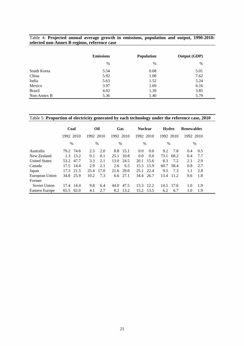
Key drivers of emissions growth in the different regions are changes in GDP, population and thecarbon intensity of output. In turn, the carbon intensity of output, measured by the ratio of aggregateemissions to aggregate output, depends critically on the shares of different fuels in electricitygeneration. Projected GDP and population growth rates are shown in tables 3 and 4. These GDPassumptions take account of the impacts on growth of the recent Asian financial crisis that started in1997. Fuel shares in electricity generation have been calibrated with projections based on informationfrom individual countries and the International Energy Agency (table 5). The shares in electricitygeneration of oil, nuclear energy and hydro power are projected to decline for most Annex B regionsby 2010. In comparison, gas use for electricity generation is projected to increase considerably inmost regions under the reference case due to technological improvements in the design, operation andefficiency of combined cycle gas turbines (IEA 1996).

Australia’s continued strong reliance on fossil fuels (particularly coal) in electricity generation;strong projected growth in exports from energy intensive industries such as iron and steel and

8

nonferrous metals; and relatively high population growth rate contribute to Australia’s above averageprojected emissions growth rate in the reference case (table 3).

Emissions growth in New Zealand and Canada is also projected to be higher than average over theperiod 1990–2010. These regions rely predominantly on nonfossil fuel intensive energy sources.However, the scope for future growth in hydro power and nuclear energy is assumed to be limited inthese countries and, therefore, the use of other more emission intensive fuels is projected to increase,thereby leading to a relatively rapid increase in emissions in the reference case.

The low projected emissions growth rates in the European Union and Japan arise for three mainreasons. First, the emissions intensity of electricity production is projected to decline significantly inthe reference case because of a shift into gas fired power generation. Second, the share in output ofemissions intensive industries such as iron and steel is projected to fall. Third, low population growthrates contribute to low growth in final consumer demand for fuel.

In contrast, the main reason for the former Soviet Union’s low projected emissions growth rate is thelow assumed average economic growth over the projection period. Emissions in the former SovietUnion are projected to be 1.5 per cent below 1990 levels at 2010.

The strong projected emissions growth in developing countries is largely a result of the strongprojected economic growth in these regions following an assumed recovery from current crisisconditions by 2001 for most Asian economies and the associated increase in fossil fuel demand. Inaddition, the share of emission intensive industries in output is projected to increase over theprojection period.

Impacts of abatement policies on Annex B countriesThere have been a number of modeling studies examining the use of global emissions trading andindependent abatement as mechanisms for achieving an emission abatement target (Manne andRichels 1991, 1995; Manne and Richels 1995; Edmonds et al. 1995; Richels et al. 1996 and Jacoby etal. 1997). Each of these studies found that the use of a global emissions trading scheme could reducethe economic costs of emission abatement. For example, Jacoby et al. (1997) used the EPPA model(Yang et al. 1996) to consider an emission abatement scenario where the Annex I regions reducedemissions to 20 per cent below 1990 levels at 2005 and held emissions fixed until 2050. By theperiod 2030–50, the economic costs of emission abatement (measured by a consumption basedwelfare index) were reduced by 60–70 per cent compared with independent abatement.

In these studies, the reduction in costs associated with emissions trading occurs because tradingequalises the marginal costs of abatement across participating regions. This will minimise the totalcosts of abatement because, if marginal costs of abatement were not equal, it would always bepossible to lower the total costs of abatement by shifting abatement to sources where the marginalcosts of abatement were lower.

An extensive theoretical and qualitative literature has developed on the topic of emissions trading andcomparisons with other policies. For example, Fisher, Barrett, Bohm, Kuroda, Mubazi, Shah andStavins (1996) contains an extensive bibliography on the literature on emissions trading before 1996.Mullins and Baron (1997) provide a nontechnical discussion of the various types of emissions tradingschemes. Rose (1997) reviews the use of tradable quota schemes for natural resource managementproblems. Hinchy et al. 1998 consider a number of design and implementation issues are critical toachieving a least cost outcome in an emissions trading scheme. Ensuring that the market for tradablepermits is competitive and that transaction costs are minimised are central to these design issues.

Measuring impactsThe carbon emission penalty for a country is the economic cost associated with making emissionreductions at the margin and it determines changes in aggregate production and trade resulting from

9

emission abatement policies. However, these penalties may not be well correlated with changes innational economic welfare resulting from emission abatement, especially when comparisons ofpenalties are made across countries. Instead, a range of macroeconomic variables has been used inrecent literature to measure the impact of climate change policies on national economic welfare.These include GDP (Manne and Richels 1998), GNP (McKibbin and Pearce 1996; Kennedy et al.1998), GNE (Brown et al. 1997), direct net cost measures (Jacoby et al. 1998), real consumption andequivalent variation (Montgomery et al. 1998).

In this paper, percentage changes in gross national product (GNP) from reference case levels are usedto measure the aggregate economic impact of emission abatement policies. GNP is equal to grossdomestic product (GDP) plus foreign income transfers, and therefore provides a complete measure ofthe flow of income available to an economy for consumption, saving and depreciation. In the contextof international emissions trading, for example, changes in GNP from reference case levels accountfor both the income transfers associated with quota purchases and sales and changes in GDP resultingfrom increases in the cost of emitting carbon.

Changes in GNP can be decomposed (to a first order approximation) into impacts from a range ofsources — the direct impact on an Annex B country of an increase in the cost of emitting carbonwithin that country; a foreign income transfer impact arising from international quota purchases andsales (if any); and a trade impact.

The trade impact arises because actions to limit emissions in Annex B countries will affect therelative prices of products traded on world markets. For example, reduced world demand for fossilfuels resulting from emission abatement in Annex B countries will reduce returns to fossil fuelproducers. This will have negative trade related impacts on net exporters of fossil fuels such asAustralia. Such trade impacts will affect output and also net returns from foreign held assets inAnnex B countries and non-Annex B countries. Such trade impacts could be large for individualcountries, depending on the composition and direction of their trade and extent of net foreign assetholdings (McKibbin and Pearce 1996; Brown et al. 1997).

Changes in real consumption resulting from the imposition of policies are used to measure changes ininstantaneous national welfare. At each point in time, national income (as measured by GNP) isdivided by final consumers (private and government) into consumption and savings. Theconsumption component of this contributes to consumer welfare at that point in time. Savings areaccumulated to fund future consumption and therefore contribute to welfare in future years. Underparticular assumptions, for a given period, changes in real consumption are a first orderapproximation of changes in national welfare resulting from a policy change (Varian 1984, p. 276).

Carbon emission penalties and emission reductionsAs noted above, the economic impacts of emission abatement policies result from the introduction ofcarbon emission penalties in Annex B countries. These penalties raise production costs in emissionintensive industries which in general leads to higher consumer prices, reducing both export anddomestic demand and therefore output levels. Estimated carbon emission penalties at 2010 andassociated emission reductions under the various scenarios are shown in table 6.

With independent emission reductions, carbon emission penalties vary substantially from country tocountry. The estimated carbon emission penalty is related to the magnitude of emission reductionrequired in a country, the ease of substitution between fuel sources with different carbon dioxideintensity, and the responsiveness of energy demand, more generally, to changes in energy costs.

When acting independently, countries are assumed to utilise least costly methods of reducingemissions first. Consequently, as the size of the emission abatement task is increased, the carbonemission penalty will tend to increase, as lower cost abatement possibilities become increasinglyscarce. Canada has the highest projected emission abatement task (when considering carbon dioxide

10

emissions from fossil fuel use) and this contributes to the relatively high marginal cost of abatementunder the Kyoto Protocol, without emissions trading.

The imposition of a carbon emission penalty will result in consumers and producers attempting tosubstitute into less emission intensive fuel sources. This fuel switching is particularly important in theelectricity sector. Substitution possibilities can be limited if a region already uses technologies in theelectricity sector that are not emission intensive. This implies a need to reduce emissions in thetransport and industrial sectors, where substitution possibilities tend to be more limited and wherehigher carbon penalties are required to encourage emission abatement. The contributions of theelectricity sector to total carbon dioxide emissions for Annex B countries are shown in figure 1. Forexample, Canada relies heavily on hydroelectricity (and to a lesser extent nuclear power) andtherefore has less scope for low cost emission reductions in the electricity sector than countries thatare less reliant on hydroelectricity.

The relatively low carbon emission penalty for eastern Europe and the zero penalty for the formerSoviet Union indicate the existence of opportunities for low cost emission reductions relative to thecosts of such reductions in other Annex B countries. For the former Soviet Union, because emissionsdo not rise above 1990 levels by 2010, that region has already undertaken abatement (contraction)sufficient to meet its commitment set out in table 1. Emissions in the former Soviet Union are abovereference case levels in this scenario as production costs rise in Annex B countries where emissionconstraints are binding, leading to some shift in carbon intensive industries from other Annex Bcountries to the former Soviet Union.

With Annex B emissions trading, carbon emission penalties in participating countries are equalised atthe Annex B emission quota price. Because trading allows more emission abatement to take place inregions where pre-trade marginal emission abatement costs are low, carbon emission penalties for allAnnex B except the former Soviet Union and eastern Europe regions are reduced relative toindependent abatement. In these regions, emission reductions rise significantly relative to the casewithout trading as they take advantage of their low cost abatement opportunities and sell emissionrights to the other Annex B countries. To compensate the former Soviet Union and eastern Europe fortaking on additional abatement, income is transferred to them from all other Annex B regions in theform of payment for emission quota. These transfers are discussed in greater detail in the followingsection.

Under the double bubble, the carbon emission penalty in the European bubble is substantially higherthan under full Annex B trading. This is because the European Union no longer has access to low costemission abatement opportunities in the former Soviet Union. Instead it must purchase moreexpensive emission quotas from eastern Europe where pre-trade carbon emission penalties (marginalabatement costs) are higher than for the former Soviet Union. The change in carbon emission penaltyfor the umbrella group is relatively small because the removal of the European Union’s demand forquotas (which would tend to reduce quota prices) is offset to some extent by the removal of a similarquantity of quota supply by eastern Europe (figure 2). The net effect is a small decrease in quotaprice for the umbrella group relative to full Annex B trading.

The decline in the carbon emission penalty under emissions trading is consistent with other analysesof the Kyoto Protocol with Annex B trading. Edmonds et al. (1998), Kainuma et al. (1998) andManne and Richels (1998) all show a considerable reduction in the carbon emission penalty forAnnex B regions, excluding Russia, under an Annex B emission trading scheme.

The magnitude of the carbon emission penalty projected under Annex B emissions trading variesconsiderable across models. The carbon emission penalty projected by the AIM model (Kainuma etal. 1998) under the Kyoto Protocol with Annex B trading is around US$70 in 1992 dollars per tonneof carbon. Edmonds et al. (1998) use the Second Generation Model to project Annex B carbonemission penalty that lies between US$72 in 1992 dollars (for a return of Annex B emissions to 1990levels at 2010) and US$109 in 1992 dollars (for a 10 per cent reduction in Annex B emissions below

11

1990 levels at 2010). Manne and Richels (1998) use the MERGE model to project a carbon emissionpenalty of slightly less than US$100 in 2010 dollars per tonne of carbon. (It should be noted that thisestimate includes the use of sinks and the clean development mechanism in conjunction withemissions trading.) This compares with a GTEM projection of US$114 in 1992 dollars per tonne ofcarbon.

Differences in the estimated carbon emission penalties between modes depend to a large extent onmodel structure, particularly the energy substitution possibilities assumed in each model. Forexample, the greater the fuel switching possibilities in a particular model the lower the carbonemission penalty is likely to be. Another important determinant of the size of the carbon emissionpenalty is the reference case emissions growth. Generally, the higher the emissions growth the higherthe marginal cost of abatement. The marginal cost of abatement is affected by output and populationgrowth and, in a number of models, assumptions about autonomous energy efficiency. Some of thekey factors determining the carbon emission penalty in the GTEM model are examined in thesensitivity analysis in the appendix.

Key macroeconomic impacts and national economic welfareTable 7 shows the GDP, GNP and consumption changes resulting from the various emissionabatement policies. The increased costs to industry associated with the carbon emission penaltiesshown above, tend to dampen economic activity as measured by real GDP. The resulting decline indemand for labor and capital reduces real returns to labor and capital (defined as the gains in outputassociated with adding an extra unit of labor and capital, respectively, to the economy), in turn,leading to reduced income (GNP) and consumption. These latter measures are indicators of nationaleconomic welfare.

The GDP impacts presented in table 8 are correlated with carbon emission penalties. For example,comparing the Annex B trading and independent abatement scenarios, reductions in GDP costs areproportional to reductions in carbon emission penalties in purchasing countries. For the former SovietUnion and eastern Europe Annex B trading imposes higher GDP costs as production declines inresponse to higher costs associated with emitting carbon.

However, in terms of GNP and consumption, emissions trading provides substantial benefits to theformer Soviet Union and eastern Europe as they receive transfers associated with quota sales. Themonetary transfers as a proportion of GNP resulting from emission quota trades are shown in figure3. At the same time, gains to purchasing countries (all in the OECD), measured in terms of GNP andconsumption are generally reduced to some extent by having to transfer income to the former SovietUnion and eastern Europe. On balance, all countries experience gains associated with tradingcompared with independent abatement.

Under the double bubble arrangement, all quota purchasing countries in the umbrella group are betteroff than under full Annex B trading. This result is directly related to the reduction in quota pricedescribed in the previous section. On the other hand, the European Union is worse off under thebubble arrangement due to its assumed inability to access low cost emission abatement opportunitiesin the former Soviet Union through trading. The increased quota price in the European bubblerelative to full Annex B trading works to the benefit of eastern Europe as its quota income isincreased, increasing GNP and consumption.

An important feature of the results presented here is that the economic impacts (on GDP, GNP andconsumption) are only partly correlated with the size of the carbon emission penalty projected underthe Kyoto Protocol, with or without emissions trading. For example, without emissions trading thecarbon penalties projected for Japan and the European Union are higher than those projected forAustralia and the United States (table 1). However, the projected economic impacts (GDP, GNP andconsumption) on Australia and the United States are higher than for Japan and the European Union.This is because, although the size of the carbon penalty is important in determining the economicimpacts of emission abatement, the extent to which a particular country relies on fossil fuels in the

12

production structure of its economy is also important. The greater a region’s emission intensity ofoutput, the more widespread the economic impacts of a carbon penalty on the use of fossil fuels arelikely to be. This implies that an accurate indicator of the impacts of a carbon penalty on GDP is thesize of the carbon penalty for the economy as a whole (carbon penalty multiplied by emissions) as apercentage of GNP (figure 4). This measure captures the combined effects of the carbon emissionpenalty and emissions intensity of output.

The availability of relatively inexpensive fossil fuels in Australia and the United States has led tohigh fossil fuel intensity in these economies. In particular, in Australia, there is a heavy reliance oncoal fired electricity generation (table 5). Consequently, the imposition of a carbon penalty will resultin relatively large increases in electricity prices. This will have widespread impacts throughout theseeconomies, leading to greater economic costs in terms of GDP, GNP and consumption. On the otherhand, Japan is relatively less emission intensive because of significant advances in energy efficiencymade in recent decades and the emission intensity of the European Union is declining due to aprojected strong growth in gas fired electricity (table 3). These types of factors now limit theavailability of further low cost emission reductions, and this is reflected in higher carbon emissionpenalties (table 6). However, the high carbon penalty associated with reducing fossil fuel use is offsetto an extent by the low fossil fuel dependence of these economies and therefore the penalty has morelimited flow on effects on competitiveness and output in Japan and the European Union than inAustralia and the United States, for example.

Impacts on developing countriesEmission abatement undertaken in Annex B regions affects non-Annex B regions primarily throughtrade impacts. First, non-Annex B fossil fuel exporters, such as Indonesia and Mexico, experience adecline in demand and prices for their fossil fuel exports which contributes negatively to total output(GDP), with adverse implications for income (GNP) and consumption (table 7). At the same time,non-Annex B fossil fuel importers, such as South Korea and Chinese Taipei, will benefit from the fallin the world price of fossil fuels. Second, the increased costs of production in Annex B regions arepassed on to consumers of Annex B products in non-Annex B regions, reducing the internationalpurchasing power of non-Annex B regions. Third, exporters in non-Annex B regions face an overalldecline in export demand as income growth in Annex B regions declines. On the positive side, non-Annex B regions, particularly China, will benefit from increased export earnings from carbonleakage.

Carbon leakage is the partial offsetting of emission reductions in abating regions by increases inemissions from nonabating regions. Leakage occurs because emission abatement increases the cost offossil fuels in Annex B regions, thereby increasing the price of fossil fuel intensive products such asiron and steel. As a result, non-Annex B producers of fossil fuel intensive products gain a competitiveadvantage over producers in Annex B regions. In response, there is a partial shift in emissionintensive industries from Annex B to non-Annex B regions. In effect, this response will intensify thetrend toward service dominated economies in Annex B regions.

Without emissions trading, non-Annex B carbon dioxide emissions from fossil fuel combustion areprojected to increase by 3.5 per cent from the reference case level at 2010. This implies a carbonleakage rate2 of 18 per cent; that is, for every one million tonnes reduction in carbon dioxideemissions in Annex B regions, carbon dioxide emissions from non-Annex B regions are projected torise by 180 000 tonnes. The extent of carbon leakage is correlated with the size of the carbonemission penalty in Annex B regions. The greater the carbon emission penalty, the greater the imposton energy intensive production in Annex B regions and the greater the loss of competitiveness againstnon-Annex B regions. With an international emissions trading scheme, non-Annex B emissions areprojected to rise 1.2 per cent above reference case levels at 2010. Therefore, the carbon leakage rate

2 The carbon leakage rate is calculated as the emissions increase projected for non-Annex B regions in

megatonnes (Mt), divided by the emission reductions in Annex B regions (Mt), multiplied by -100.

13

is lower with trading (6 per cent) as Annex B regions face, on average, a lower carbon emissionpenalty.

Under the double bubble scenario, non-Annex B emissions are projected to increase 1.4 per centabove reference case levels at 2010. The carbon leakage rate under the double bubble arrangement (8per cent) is reduced compared with leakage when there is no trading. However, carbon leakage is stillslightly higher under the double bubble than under Annex B trading as increased abatement costs inthe European Union and eastern Europe lead to more leakage from countries that compete with theseregions in the production of emission intensive products. These regions include China, Korea andcountries in the ‘rest of world’ region which includes the African and Middle Eastern economies thathave significant trade with the European Union.

A number of multiregion models have been used to estimate carbon leakage rates (Martin et al. 1992;Pezzey 1992; Oliveira-Martins, Burniaux and Martin 1992; Manne and Oliveira-Martins 1994;Edmonds, Wise and Barns 1995; Golombek, Hagen and Hoel 1995 and Jacoby 1997). Carbon leakagerates range from close to zero (Martin et al. 1992 using the GREEN model) to 70 per cent (Pezzey1992 using the Whalley–Wigle model). GTEM estimates lie at the lower end of this range. However,differences in regional and sectoral detail make intermodel comparisons of carbon leakage ratesproblematic.

ConclusionThere is still significant uncertainty surrounding the Kyoto Protocol for a number of reasons. First,much of the detail in the protocol remains to be negotiated. For example, the details of emissionstrading and the way in which the clean development mechanism will work are yet to be formulated.Much also remains to be done in terms of defining the way in which sinks will be used in assistingcountries to meet their targets. Second, uncertainty still remains about the timing of the entry intoforce of the protocol and the implications that may have for the size of the adjustment costsassociated with meeting the target for the first commitment period.

Despite the uncertainty, the decisions taken at Kyoto have changed the growth path for the worldeconomy forever. Governments have already moved to implement policies to reduce emissions andindustries have already responded. But a great deal remains to be done in designing the policies thatminimise the economic costs of achieving the targets already agreed. Emissions trading, and the otherflexibility mechanisms allowed for in the protocol, provide one way of minimising the costs andcoincidently increase the environmental effectiveness of the Protocol. The acceptance of the so-calledflexibility mechanisms as legitimate instruments is one of the primary keys to the successfulimplementation of the Kyoto Protocol.

14

Appendix: Sensitivity analysis

Sensitivity of the carbon emission penalty to model assumptions aboutrestrictions on electricity technologiesIn GTEM, estimates of marginal emission abatement costs are particularly sensitive to assumptionsabout restrictions on the expansion of hydroelectricity and nuclear power for electricity generation.

Estimates of marginal emission abatement costs under Annex B emission trading with alternativeassumptions regarding possible growth in hydro and nuclear power are presented in figure 5.

Under the ‘all Annex B constrained’ simulation, hydro and nuclear power are not permitted to growabove reference case levels for the former Soviet Union and eastern Europe. The ‘nuclearunconstrained’ result is based on the assumption that electricity production using nuclear power inthe OECD is allowed to increase above reference case levels under the policy simulations but thathydroelectricity remains constrained as in the standard assumptions. This implies that the onlybarriers to the expansion of nuclear power relate to cost. The Annex B unconstrained case assumesno restriction on growth above reference case levels on the quantity of either hydroelectricity andnuclear power in OECD regions. In particular for hydro electricity this assumption means that it ispossible (at least in a modelling context) to expand hydroelectricity production without regard to anyabsolute limit on the availability of sites for hydroelectricity projects. The only constraint onhydroelectric expansion is represented by electricity supply production costs which increase at anincreasing rate as hydro capacity is increased.

The carbon emission penalty is projected to be around 28 per cent lower under the Annex Bunconstrained case than under the standard assumptions. Making additional hydro and nuclearcapacity available for Annex B regions increases the potential for emission abatement to beundertaken by fuel switching. Ignoring the absolute physical constraints on the expansion of hydropower and the political constraints, Annex B regions are able to substitute ‘fossil fuel free’ electricitygeneration technologies for fossil fuel based technologies at a lower cost than was possible under thestandard assumptions. This, in turn, lowers the carbon emission penalty needed to meet given targets.

The results indicate that removing the assumed nuclear constraint on OECD regions decreases thecarbon emission penalty by 23 per cent compared with standard assumptions. The relaxation of thehydro constraint as well is projected to reduce the carbon emission penalty by a further 7 per cent.The importance of the nuclear constraint in determining carbon emission penalties is due to relativelyhigh costs associated with substantial expansion of hydro power in a number of large OECDcountries such as the United States, Japan and the European Union.

By including constraints on hydro and nuclear power in the former Soviet Union and eastern Europe,the carbon emission penalty under trading is projected to increase by 13 per cent. This is because of areduction in the availability of low cost emission reduction opportunities in these regions and asubsequent increase in the price that would be need to be paid to them to reduce emissions.

The unconstrained case mimics the features of the approach used to modeling energy substitution inthe energy sector in the majority of general equilibrium models used to analyse climate change issues.In this case, capital and labor use in electricity production are permitted to expand without bound.Brown et al. (1996) have shown that such an approach leads to technologically infeasible electricitymixes. Also, significant increases in capital and labor usage could imply expansion in renewablepower forms including hydro and nuclear that may not be feasible from a physical or politicalperspective.

At the regional level, imposing constraints on hydro and nuclear power is projected to increase thecarbon emission penalty. The carbon emission penalty under independent emission abatement given

15

various assumptions about technology constraints on the United States is shown in figure 6. Theresults show that the carbon emission penalty falls when the restrictions are removed. The mostsignificant constraint in terms of raising the abatement cost is that placed on nuclear power. If it isremoved the carbon emission penalty falls by 40 per cent. Further, removing the constraint onhydroelectricity reduces the carbon emission penalty by 10 per cent.

The magnitude of the carbon emission penalty projected for the United States under the KyotoProtocol without emissions trading varies across models. For example, the carbon emission penaltyprojected by the AIM model (Kainuma et al. 1998) for the United States is around US$160 in 1992dollars per tonne of carbon. The estimate from Edmonds et al. (1997) lies between US$108 in 1992dollars (for a return of Annex B emissions to 1990 levels at 2010) and US$173 in 1992 dollars (for a10 per cent reduction in Annex B emissions below 1990 levels at 2010). Manne and Richels (1998)use the MERGE model to project a carbon emission penalty of slightly less than US$240 in 2010dollars per tonne of carbon. This compares with GTEM projection of US$345 in 1992 dollars pertonne of carbon which is at the upper end of the majority of estimates. Interestingly, the carbonemission penalty projected in the unconstrained case of US$187 in 1992 dollars per tonne of carbonis within the range of the majority of other estimates.

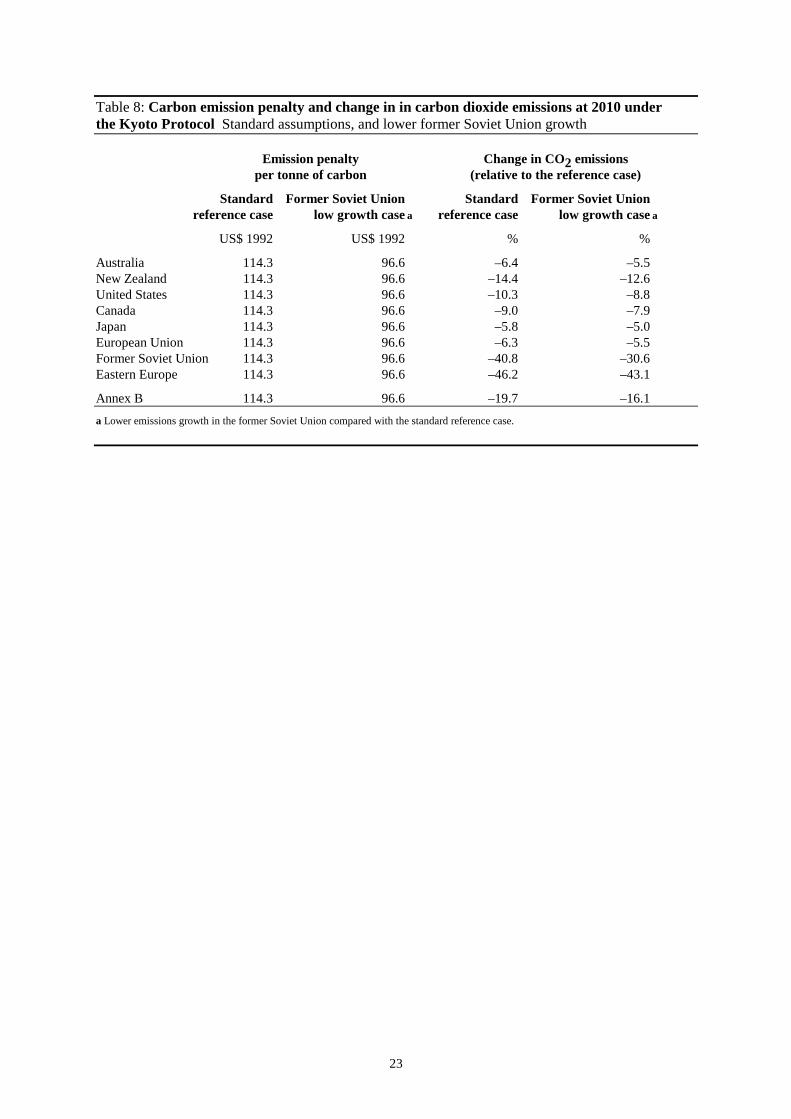
Sensitivity of the carbon emission penalty to model assumptions aboutformer Soviet Union emissions growthReference case emissions growth are an important determinant of the marginal cost of abatement in agiven region. Considerable uncertainty surrounds reference case emissions growth in the formerSoviet Union because of the uncertainty about economic growth in that region. As the former SovietUnion is projected to be the main supplier of emission quotas under the Annex B trading scenario,changes in the reference case emissions growth in the former Soviet Union are likely to haveconsiderable impacts on the Annex B carbon emission penalty under an emissions trading scheme.

For example, with lower growth in emissions, the quantity of emissions quota available for sale bythe former Soviet Union will increase. This increase in supply will tend to reduce the internationalprice of emission quotas and, therefore, lower the Annex B carbon emission penalty under anemissions trading scheme.

The projected emissions growth in the standard GTEM reference case declines at an average annualgrowth of 0.08 per cent between 1990–2010 (table 3). A second reference case has been undertakenusing emission projections from the IEA (1998) that decline at an average annual rate of 1.35 percent. This is significantly lower than the emissions growth projected under standard GTEMassumptions and reflects the uncertainty surrounding future developments in the former SovietUnion.

The projected carbon emission penalty under the Kyoto Protocol with emissions trading withstandard reference case assumptions and lower emissions growth in the former Soviet Union arepresented in table 8. With lower emissions growth the carbon emission penalty is reduced and theformer Soviet Union can sell more quota to other Annex B regions. This lowers the internationalquota price.

16

ReferencesABARE 1996, The MEGABARE Model: Interim Documentation, Canberra

Armington, P.S. 1969a, ‘A theory of demand for products distinguished by place of production’, IMFStaff Papers, vol. 16, no. 2, pp. 159–78.

—— 1969b, The geographic pattern of trade and the effects of price changes, IMF Staff Papers, vol.16, no. 2, pp. 179–201

Brown, S., Donovan, D., Fisher, B., Hanslow, K., Hinchy, M., Matthewson, M., Polidano, C.,Tulpulé, V. and Wear, S. 1997, The Economic Impact of International Climate Change Policy,ABARE Research Report 97.4, Canberra.

Burniaux, J-M., Martin, J., Nicoletti, G. and Martins, J. 1991, GREEN — A Multi-region, DynamicGeneral Equilibrium Model for Quantifying the Costs of Curbing CO2 Emissions: A Technical

Manual, Department of Economics and Statistics Working Paper 104, OECD, Paris.

Burnstein, P., Montgomery, D. and Rutherford, T. 1996, The International Impacts AssessmentModel, University of Colorado and Charles River Associates Incorporated, Washington DC.

Edmonds, J., Kim, S., MacCracken, C., Sands, R. and Wise, M. 1998, Return to 1990: The cost ofmitigating United States carbon emissions in the post-2000, Paper presented at the EnergyModeling Forum Meeting, Snowmass, Colorado, August 10–11.

——, Pitcher, H.M., Barns, D., Baron, R. and Wise, M.A. 1995, ‘Modeling future greenhouse gasemissions: the second generation model description’, in Modeling Global Change, United NationsUniversity Press, Tokyo.

——, Wise, M. and Barns, D.W. 1995, ‘Carbon coalitions: the cost effectiveness of energyagreements to alter trajectories of atmospheric carbon dioxide emissions, Energy Policy, vol. 23,no. 4. pp. 309–35.

—— and Reilly, J. 1983, ‘Global energy and CO2 to the year 2050’, Energy Journal, vol. 3, no. 4,

pp. 21–47

Fisher, B., Barrett, S., Bohm, P., Kuroda, M., Mubazi, J., Shah, A. and Stavins, R. 1996, ‘Aneconomic assessment of policy instruments for combatting climate change’, in IPCC, SecondAssessment Report, Working Group III, Cambridge University Press, Massachusetts, pp. 401–33.

Golombek, R., Hagen, C. and Hoel, M. 1995, ‘Efficient incomplete international climateagreements’, Resource and Energy Economics, vol. 17, no. 1, pp. 25–46.

Hinchy, M., Hanslow, K., Fisher, B.S. and Graham, B. 1998, International Trading in GreenhouseGas Emissions: Some Fundamental Principles, ABARE Research Report 98.3, Canberra.

Hertel, T. (ed.) 1997, Global Trade Analysis: Modeling and Applications, Cambridge UniversityPress, Massachusetts

IEA (International Energy Agency) 1994, Electricity Information 1994, OECD, France.

—— 1996, World Energy Outlook 1996 Edition, OECD, France.

—— 1998, International Energy Outlook 1998, Washington DC.

IISI (International Iron and Steel Institute) 1996, Steel Statistics Yearbook 1996, Committee onEconomic Studies, Brussels.

17

Industry Commission 1991, Costs and Benefits of Reducing Greenhouse Gas Emissions, Report no.15, AGPS, Canberra.

Jacoby, H., Schmalenese, R. and Wing, I.S. 1998, Toward a useful architecture for climate changenegotiations, Paper presented at the Energy Modeling Forum Meeting, Snomass, Colorado, August10–11.

Jacoby, H., Eckhaus, R., Ellerman, A., Prinn, R., Reiner, D. and Yang, Z. 1997, ‘CO2 emissionlimits: economic adjustments and the distribution of burdens’, Energy Journal, vol. 18, no. 3, pp.31–58.

Kainuma, M., Matsuoka, Y., Mortia, T. and Masui, T. 1998, Preliminary analysis of post-Kyoto EMFscenarios, Paper presented at the Energy Modeling Forum Meeting, Snomass, Colorado, August10–11.

Kennedy, D., Polidano, C., Lim, J. and Fisher, B.S. 1998, Climate change policy and the economicimpact of the Kyoto Protocol, ABARE conference paper 98.23 presented at the South AustralianOffice of Energy Policy Opportunities Out of Kyoto Conference, Adelaide, 1 September.

McDougall, R. (ed.) 1997, Global Trade, Assistance, and Protection: The GTAP 3 Data Base, Centerfor Global Trade Analysis, Purdue University.

McKibbin, W. and Wilcoxen, P. 1992, G-CUBED: A Dynamic Multisectoral General EquilibriumModel of the Global Economy, Brookings Discussion Paper in International Economics no. 128,Brookings Institution, Washington DC.

McKibbin, W. and Pearce, D. 1996, ‘Global carbon taxes: an Australian perspective’, in Bouma,W.S., Pearman, G.I. and Manning, M.R. (eds), Greenhouse: Coping with Climate Change, CSIRO,Melbourne, pp. 510–85.

Manne, A., and Oliveira-Martins, J. 1994, ‘Comparison of model structure and policy scenarios:GREEN and 12RT’, OECD Economics Department Working Paper No. 146, Paris.

——, Medelsohn, R. and Richels, R. 1995, ‘MERGE: A model for evaluating regional and globaleffects of GHG reduction policies’, Energy Policy, vol. 23, no. 1.

Manne, A and Richels, R. 1998, The Kyoto Protocol: A cost-effective strategy for meetingenvironmental objectives?, Paper presented at the Energy Modeling Forum Meeting, Snomass,Colorado, August 10–11.

—— 1995, ‘The greenhouse debate: economic efficiency, burden sharing and hedging strategies’,Energy Journal, vol. 16, no. 4, pp. 1–37.

—— 1992, Buying Greenhouse Insurance — The Economic Cost of CO2 Emission Limits, MIT

Press, Cambridge, Massachusetts.

—— 1991, ‘International trade in carbon emission rights: a decomposition procedure’, AmericanEconomic Review: Papers and Proceedings, vol. 81, no. 2, pp 136–9.

Martin, J., Burniaux, J-M., Nicoletti, G. and Oliveira-Martins, J. 1992, ‘The cost of internationalagreements to reduce CO2 emissions: evidence from GREEN’, OECD Economic Studies, no. 19,Winter, pp. 92–121.

Montgomery, D. 1972, Markets in licences and efficient pollution control programs, Journal ofEconomic Theory, vol. 5. pp. 101–115

Montgomery, W.D. 1997, ‘Impacts of Annex 1 actions on non-Annex 1 countries’, Presentation at theIPCC Workshop, August 18 1997, Oslo.

18

Mullins, F. and Baron, R. 1997, International GHG emission trading, Policies and Measures forCommon Action Working Paper 9, Annex I Expert Group on the UN Framework Convention onClimate Change.

Oliveira-Martins, J., Burniaux, J-M. and Martin, J. 1992, ‘Trade and the effectiveness of unilateralCO2 -abatement policies: evidence from GREEN’, OECD Economic Studies 19, Paris, pp. 93–121.

Pezzey, J. 1992, ‘Analysis of unilateral CO2 control in the European Community and the OECD’,Energy Journal, vol. 13, no. 3, pp. 159–71.

Richels, R., Edmonds, J., Gruenspecht, H. and Wigley, T. 1996, ‘The Berlin Mandate: The design ofcost-effective strategies’, Paper presented at the Stanford Energy Modeling Forum, February 3,1996.

Rose, R. 1997, ‘Tradable quotas for efficient natural resource use’ in Outlook 97, Proceedings of theNatural Agriculture and Resources Outlook Conference, Canberra 4–6 February, vol. 1, CommodityMarkets and Resource Management, ABARE, Canberra, pp. 107–115.

Rutherford, T. 1993, ‘The welfare effects of fossil fuel carbon restrictions: results from a recursivedynamic trade model’, in The Costs of Cutting Carbon Emissions: Results from Global Models,OECD, Paris.

Whalley, J and Wigle, R. 1991, ‘The international incidence of carbon taxes’, in Dornbush, R. andPorterba, J. (eds), Economic Policy Response to Global Warming, MIT Press, Cambridge,Massachusetts.

Yang, Z. et al. 1996, The MIT Emissions Prediction and Policy Assessment (EPPA) Model, MIT JointProgram on the Science and Policy of Global Change, Report no. 6, MIT Press, Cambridge,Massachusetts.

United Nations 1992, World Population Prospects 1992, Magnetic tape, Pro233, New York.

—— 1993, Kyoto Protocol to the United Nations Framework Convention on Climate Change,http://www.unfcc.de/

—— 1994a, Industrial Statistics Yearbook 1994, Volume I, General Industrial Statistics, UnitedNations, New York.

—— 1994b, Industrial Statistics Yearbook 1994, Volume II, Commodity Production Statistics,United Nations, New York.

Varian, H. 1994, Microeconomic Analysis, 2nd edn, Norton and Coy, New York.

19

Table 1: Kyoto Protocol target commitments for Annex B countries

Party Target Party Target(percentage of base year or period) (percentage of base year or period)

Australia 108 Lithuania 92Austria 92 Luxembourg 92Belgium 92 Monaco 92Bulgaria 92 Netherlands 92Canada 94 New Zealand 100Croatia 95 Norway 101Czech Republic 92 Poland 94Denmark 92 Portugal 92Estonia 92 Romania 92European Community 92 Russian Federation 100Finland 92 Slovakia 92France 92 Slovenia 92Germany 92 Spain 92Greece 92 Sweden 92Hungary 94 Switzerland 92Iceland 110 Ukraine 100Ireland 92 United Kingdom of GreatItaly 92 Britain and Northern Ireland 92Japan 94 United States of America 93Latvia 92Liechtenstein 92

Source: United Nations (1998).

20

Table 2: Regional and commodity coverage

Regions Commodities

1 Australia 1 Coal2 New Zealand 2 Oil3 United States 3 Natural gas4 Canada 4 Other minerals5 Japan 5 Petroleum products6 European Union (15) a 6 Chemicals, plastics7 South Korea 7 Nonmetallic minerals8 China 8 Iron and steel9 Chinese Taipei 9 Nonferrous metals10 Indonesia 10 Fabricated metal products11 Other ASEAN 11 Electricity12 India 12 Primary agriculture13 Mexico 13 Processed agriculture14 Brazil 14 Resources processing15 Rest of America 15 Manufacturing16 Former Soviet Union 16 Services17 Eastern Europe c18 Rest of world

a Comprises Austria, Belgium, Denmark, Finland, France, Germany, Greece, Ireland, Italy, Luxembourg, The Netherlands, Portugal, Spain,Sweden and the United Kingdom. b Comprises Switzerland, Norway and Iceland. c Comprises Bulgaria, Czech Republic, Hungary, Poland,Romania, Slovakia and Slovenia.

Table 3: Projected annual average growth in emissions, population and output, 1990-2010:Annex B regions, reference case

Emissions Population Output (GDP)

% % %

Australia 1.79 1.15 3.43New Zealand 1.83 0.74 2.96United States 1.26 0.71 2.66Canada 1.57 0.93 2.70Japan 0.92 0.23 3.17European Union 1.05 0.21 2.84Former Soviet Union –0.08 0.42 0.80Eastern Europe 0.99 0.33 2.51Annex B average 0.85 0.41 2.76

21

Table 4: Projected annual average growth in emissions, population and output, 1990-2010:selected non-Annex B regions, reference case

Emissions Population Output (GDP)

% % %

South Korea 5.54 0.68 5.01China 5.92 1.08 7.62India 5.63 1.52 5.24Mexico 3.97 1.69 6.16Brazil 4.02 1.39 3.85Non-Annex B 5.36 1.40 5.79

Table 5: Proportion of electricity generated by each technology under the reference case, 2010

Coal Oil Gas Nuclear Hydro Renewables

1992 2010 1992 2010 1992 2010 1992 2010 1992 2010 1992 2010

% % % % % %

Australia 79.2 74.6 2.3 2.0 8.8 15.1 0.0 0.0 9.2 7.8 0.4 0.5New Zealand 1.3 13.2 0.1 0.1 25.1 10.8 0.0 0.0 73.1 68.2 0.4 7.7United States 53.2 47.7 3.3 2.1 13.0 24.5 20.1 15.6 8.3 7.2 2.1 2.9Canada 17.5 14.4 2.9 2.1 2.6 6.5 15.5 15.9 60.7 58.4 0.8 2.7Japan 17.3 21.5 25.4 17.0 21.6 29.0 25.1 22.4 9.5 7.3 1.1 2.8European Union 34.8 25.9 10.2 7.3 6.6 27.1 34.4 26.7 13.4 11.2 0.6 1.8Former Soviet Union 17.4 14.4 9.8 6.4 44.0 47.5 13.3 12.2 14.5 17.6 1.0 1.9Eastern Europe 65.5 62.0 4.1 2.7 8.2 13.2 15.2 13.5 6.2 6.7 1.0 1.9

22

Table 6: Carbon emission penalties and projected change in carbon dioxide emission reductionsat 2010 under the Kyoto Protocol Three emission trading scenarios

Emission penalty Change in CO2 emissionsper tonne of carbon (relative to the reference case)

Independent Annex B Double Independent Annex B Doubleabatement trading bubble abatement trading bubble

US$ 1992 US$ 1992 US$ 1992 % % %

Australia 455 114 108 –24.2 –6.4 –6.0New Zealand 396 114 108 –30.4 –14.4 –13.7United States 346 114 108 –27.6 –10.3 –9.7Canada 835 114 108 –31.2 –9.0 –8.5Japan 693 114 108 –21.8 –5.8 –5.4European Union 714 114 176 –25.3 –6.3 –9.2Former Soviet Union 0 114 108 1.6 –40.8 –37.1Eastern Europe 40 114 176 –23.6 –46.2 –53.6

Annex B 322 114 126 –19.7 –19.7 –19.7

Table 7: Projected change in real GDP, GNP and consumption at 2010 under the KyotoProtocol:relative to the reference case

Real GDP Real GNP Real consumption

Indepen- Indepen- Indepen-dent dent dent

abate- Annex B Double abate- Annex B Double abate- Annex B Doublement trading bubble ment trading bubble ment trading bubble

% % % % % % % % %

Australia –1.3 –0.1 –0.1 –1.4 –0.7 –0.6 –1.5 –0.6 –0.5New Zealand –2.7 –1.3 –1.2 –2.1 –1.2 –1.1 –2.7 –1.4 –1.3United States –2.0 –0.4 –0.4 –2.0 –1.1 –1.0 –2.1 –1.0 –0.9Canada –2.3 –0.3 –0.2 –2.2 –1.0 –0.9 –2.9 –1.0 –0.9Japan –0.7 0.0 0.0 –0.8 –0.3 –0.3 –0.4 –0.2 –0.2European Union –0.9 –0.1 –0.2 –0.9 –0.2 –0.4 –1.0 –0.3 –0.4Former Soviet Union 0.0 –1.9 –1.8 0.5 9.1 8.1 0.1 6.4 5.7Eastern Europe –0.5 –1.9 –2.8 0.4 2.5 4.7 –0.1 1.6 3.4

Annex B –1.2 –0.3 –0.3 –1.2 –0.3 –0.3 –1.3 –0.3 –0.3

South Korea 0.0 0.0 0.0 0.3 0.1 0.1 0.0 0.0 0.0China 0.3 0.1 0.1 0.7 0.2 0.2 0.5 0.1 0.1Chinese Taipei 0.1 0.0 0.0 –0.4 –0.1 –0.1 –0.5 –0.1 –0.1Indonesia –0.2 0.0 0.0 –1.1 –0.3 –0.3 –1.0 –0.3 –0.3ASEAN –0.3 –0.1 –0.1 –1.2 –0.5 –0.5 –1.1 –0.3 –0.4India 0.0 0.0 0.0 0.4 0.2 0.2 0.0 0.0 0.0Mexico –0.2 0.0 0.0 –0.3 –0.1 –0.1 –0.3 0.0 0.0Brazil 0.1 0.1 0.1 0.5 0.1 0.2 –0.1 0.0 0.0Rest of America –0.1 0.0 0.0 0.5 0.2 0.2 0.3 0.1 0.1Rest of world 0.1 0.0 0.0 –0.1 0.0 0.0 –0.1 –0.1 0.0

Non-Annex B 0.04 0.02 0.03 0.0 0.0 0.0 –0.1 0.0 0.0

23

Table 8: Carbon emission penalty and change in in carbon dioxide emissions at 2010 underthe Kyoto Protocol Standard assumptions, and lower former Soviet Union growth

Emission penalty Change in CO2 emissionsper tonne of carbon (relative to the reference case)

Standard Former Soviet Union Standard Former Soviet Unionreference case low growth case a reference case low growth case a

US$ 1992 US$ 1992 % %

Australia 114.3 96.6 –6.4 –5.5New Zealand 114.3 96.6 –14.4 –12.6United States 114.3 96.6 –10.3 –8.8Canada 114.3 96.6 –9.0 –7.9Japan 114.3 96.6 –5.8 –5.0European Union 114.3 96.6 –6.3 –5.5Former Soviet Union 114.3 96.6 –40.8 –30.6Eastern Europe 114.3 96.6 –46.2 –43.1

Annex B 114.3 96.6 –19.7 –16.1

a Lower emissions growth in the former Soviet Union compared with the standard reference case.