an economic analysis of the determinants license …
TRANSCRIPT
AN ECONOMIC ANALYSIS OF THE DETERMINANTS
OF MONTANA ALCOHOL RETAIL
LICENSE PRICES
by
James Michael Banovetz, III
A thesis submitted in partial fulfillmentof the requirements for the degree
of
Master of Science
in
Applied Economics
MONTANA STATE UNIVERSITYBozeman, Montana
May 2014

©COPYRIGHT
by
James Michael Banovetz, III
2014
All Rights Reserved

ii
ACKNOWLEDGEMENTS
I would like to first thank my committee chair, Dr. Randal Rucker, and my
committee members, Dr. D. Mark Anderson and Dr. Timothy Fitzgerald. Their input and
guidance was indispensable in the thesis writing process. I would also like to thank Ms.
Denise Brunett and Ms. Shauna Helfert, from the Montana Department of Revenue; Ms.
Angela Nunn, from the Montana Department of Justice; and Mr. Neil Peterson, from the
Gaming Industry Association of Montana. They were all very patient and provided a great
deal of assistance in acquiring data and knowledge of institutional details. Finally, I would
like to thank my family and friends for their love and support. Their efforts made the
process far more enjoyable.

iii
TABLE OF CONTENTS
1. INTRODUCTION........................................................................................ 1
2. BACKGROUND.......................................................................................... 4
History ..................................................................................................... 4License Descriptions ................................................................................... 7
3. LITERATURE .......................................................................................... 15
Economics of Alcohol ............................................................................... 15Supporting Literature ................................................................................ 18
4. THEORY ................................................................................................. 22
The Competitive Market Model ................................................................... 22Quota for Licenses .................................................................................... 24Market Differentials .................................................................................. 26Application of the Model............................................................................ 27
5. DATA AND METHODOLOGY .................................................................... 35
Data....................................................................................................... 35Empirical Methodology ............................................................................. 47
6. RESULTS ................................................................................................ 68
Baseline Specifications .............................................................................. 68Subsamples ............................................................................................. 74Alternative Functional Forms ...................................................................... 79Fixed Effects ........................................................................................... 83Additional Robustness Checks..................................................................... 89
7. CONCLUSION AND DISCUSSION ............................................................ 115
Implications of the Study........................................................................... 115Possibilities for Future Analysis.................................................................. 117
REFERENCES CITED ................................................................................. 120
APPENDICES............................................................................................. 125
APPENDIX A: Timeline ........................................................................... 126APPENDIX B: Quota Formulas.................................................................. 128
iv
TABLE OF CONTENTS – CONTINUED
APPENDIX C: Comparative Statics Results .................................................. 130APPENDIX D: Variable Definitions ............................................................ 134APPENDIX E: Alternative Clusters ............................................................. 136

v
LIST OF TABLES
Table Page
1. Number of Omitted Observations, by Type ........................................... 53
2. Number of Usable Observations, by County and Year ............................. 54
3. Average All-Beverage License Price (Nominal), By City and Year ............. 55
4. Household Median Income (Nominal), by County .................................. 56
5. Unemployment, by County................................................................ 57
6. Annual Population Growth Rate, by City.............................................. 58
7. University Enrollment, by City/County ................................................ 59
8. Hotel Tax Revenue (Nominal), by County ............................................ 60
9. Video Gambling Tax Revenue (Nominal), by City .................................. 61
10. All-Beverage License Quota and Licenses Issued ................................... 62
11. Beer and Wine License Quota and Licenses Issued ................................. 63
12. Restaurant Beer and Wine License Quota and Licenses Issued .................. 64
13. Means and Standard Deviations, by Year .............................................. 66
14. Means and Standard Deviations, by City .............................................. 67
15. Determinants of License Price (Log-Level) ........................................... 97
16. Determinants of License Price (Log-Level, Restricted Observations) .......... 98
17. Determinants of License Price (Log-Level, All-Beverage Only) ................ 99
18. Determinants of License Price (Level-Level) ........................................ 100
19. Determinants of License Price (Log-Log) ............................................ 101

vi
LIST OF TABLES – CONTINUED
Table Page
20. Determinants of License Price (Log-Level, Area & Year Fixed Effects)...... 102
21. Determinants of License Price (Level-Level, Area & Year Fixed Effects) ... 103
22. Determinants of License Price (Log-Log, Area & Year Fixed Effects)........ 104
23. Determinants of Licenses Issued........................................................ 113
24. Determinants of Licenses Issued (Area Fixed Effects) ............................ 114
25. All-Beverage Quota Formula ............................................................ 129
26. Beer and Wine Quota Formula .......................................................... 129
27. Restaurant Beer and Wine Quota Formula ........................................... 129
28. Resort All-Beverage Quota Formula................................................... 129
29. Variable Definitions ........................................................................ 135
30. Alternative Clusters ........................................................................ 137

LIST OF FIGURES
Figure Page
1. Positive, Negative, and Zero Proft ....................................................... 32
2. Market, Firm, and License Market ...................................................... 33
3. Market Differentials......................................................................... 34
4. Distribution of License Prices (2005 Dollars) ........................................ 65
5. Distribution of Log License Prices (2005 Dollars) .................................. 65
6. Log-Level, Fitted Values and Gambling Revenue .................................. 105
7. Level-Level, Fitted Values and Gambling Revenue ................................ 105
8. Log-Log, Fitted Values and Log Gambling Revenue .............................. 106
9. Log-Level, Fitted Values and Median Income....................................... 106
10. Level-Level, Fitted Values and Median Income..................................... 107
11. Log-Log, Fitted Values and Log Median Income................................... 107
12. Log-Level, Fitted Values and Hotel Revenue ........................................ 108
13. Level-Level, Fitted Values and Hotel Revenue ...................................... 108
14. Log-Log, Fitted Values and Log Hotel Revenue .................................... 109
15. Residuals, by Quota Area................................................................. 109
16. Residuals, by County ...................................................................... 110
17. Residuals, by Alternative Cluster Area................................................ 110
18. Residuals, by Year .......................................................................... 111
19. Residuals, by Gambling Revenue....................................................... 111
vii

viii
LIST OF FIGURES – CONTINUED
Figure Page
20. Residuals, by Income ...................................................................... 112
21. Residuals, by Hotel Revenue ............................................................ 112
22. Timeline of MT Alcohol Laws .......................................................... 127

ix
ABSTRACT
In Montana, there are a wide array of different alcohol retail license types. Thethree major types of retail licenses for on-premises consumption are all-beverage, beer andwine, and restaurant beer and wine. The state limits the number of available licenses ofeach type, employing city-level quotas for incorporated areas and county-level quotas forunincorporated areas. The licenses may trade freely within each quota area, but generallymay not be trade between areas. Differing conditions in each quota area leads to largedifferences in license prices between the various markets. To help explain the differencesin price, the study lays out a theoretical model regarding license values. It then tests themodel’s predictions using license price data from the Montana Department of Revenue.Empirical results are calculated using ordinary least squares, finding that gamblingrevenue, university enrollment, income, and tourism are all significant determinants oflicense price. Additionally, the individual license characteristics are statistically andeconomically significant. These results support the theoretical predictions, providingevidence that the model is an appropriate way to think about the license system.
1
INTRODUCTION
Alcohol is unique among vice products in that it has unequivocally received the
most attention on a national scale in the United States. With the 18th Amendment to the
United States Constitution, Prohibition began in 1920, effectively banning the retail sale
of alcohol. Even after the ratification of the 21st Amendment, which once again legalized
sales in 1933, alcohol production and sales have remained highly regulated. Indeed, every
state in the United States continues to license and regulate all businesses that deal in
alcohol—manufacturers, wholesalers, and retailers alike. The degree to which states
intervene in the market, however, varies a great deal. For example, Nevada leaves most of
the regulation to the individual counties. In contrast, seventeen states are “control states,”
where the state directly controls distribution for certain types of alcohol.1 Usually, control
states hold monopolies over wholesale markets for liquor, frequently defined by alcohol
content—either alcohol by volume (ABV) or alcohol by weight (ABW). In some cases,
control states own and operate liquor stores as well. In non-control states, manufacturers
must sell to wholesalers in most cases, but the state does not directly handle distribution at
any level.
Montana is one of the seventeen control states, maintaining a monopoly on the
sales of liquor, fortified wine, and beer with high alcohol content at the wholesale level.2
At the retail level, the Montana Department of Revenue issues many types of retail
licenses subject to a quota system. Once issued, state law permits owners to transfer
1Maryland has control counties, but is not a control state per se.2High alcohol beer is defined as having an alcohol content of at least 14% ABV.

2
licenses. Given that the state limits the number of licenses in use, most businesses must
purchase a license from a current license owner. The license prices, however, vary widely
across license types market areas. While licenses in some markets sell at prices not far
above the small annual licensing fees, licenses in others routinely sell at six-figure prices.
The highest prices observed in this study were from transfers in Billings, Bozeman, and
Missoula, with several all-beverage licenses selling at prices of $1,000,000 each in recent
years.
The large disparities in prices between locations and license type lead to several
interesting questions, including how prices are determined. To answer this question, the
analysis begins by constructing a competitive market model, with the addition of a quota
limiting the number of establishments. This basic framework is well established—the
introduction of tradable permits in competitive taxi cab markets is literally a textbook
example (Hyman 1986). The implications of model, however, have not been rigorously
derived or tested empirically, particularly with respect to alcohol retail licenses.
To test the implications of the model, OLS regressions are employed using
public-access license price data from the Montana Department of Revenue. Within the
department, the Liquor Control Division regulates and tracks license transfers (among
other regulatory responsibilities), maintaining a database of all transactions. In addition to
the systematic differences in price across the various license types, the results indicate that
several other demand factors offer significant explanatory power in pricing licenses.
Particularly, gambling, enrollment, and income all show strong positive relationships with
the market value of alcohol licenses. Although the relationship is slightly weaker, tourism

3
appears to be another important predictor of license price. The results are robust to both
functional form and the inclusion of controls for the supply of licenses (alleviating
concerns of simultaneity bias). The effects largely rely on cross-sectional variation,
causing results to be sensitive to functional form if geographic fixed effects are included.
The analysis provides value in two ways. First, it contributes to the literature by
developing and empirically testing an existing theory in a new context. Second,
understanding the determinants of price in each license market has implications for
businesses, e.g., retail establishments and financial institutions. Price determination is a
relevant issue, particularly considering that liquor licenses may be used as collateral for
loans. Additionally, given the involvement of government in the alcohol industry,
examining what economic and social characteristics affect license prices is important in
informing policy discussion.
4
BACKGROUND
History
Prior to Prohibition, Montana had relatively few regulations regarding the issuance
of alcoholic beverage licenses; all that the state required was a licensing fee (Revenue
Oversight Committee 1980). Once Congress voted to enact Prohibition, however,
Montana moved relatively quickly, becoming the seventh state to ratify the 18th
Amendment to the United States Constitution on February 19th, 1918. Along with the rest
of the United States, the retailing of alcoholic beverages was effectively illegal in Montana
between 1920 and 1933. When the United States repealed Prohibition through the
ratification of the 21st Amendment in 1933 (Montana did not ratify it until 1934), the state
created the Montana Liquor Control Board to regulate alcohol sales (Congressional
Research Service 2004).3
Modeling their control system on that of Alberta, Montana owned and operated all
package alcohol stores in the state. The Liquor Control Board (LCB) maintained a
monopoly on all liquor sales, with bars and taverns limited to serving beer (Quinn 1970).4
In 1937 the legislature passed House Bill 196, which permitted liquor-by-the-drink sales
in licensed establishments statewide. To acquire a license to serve liquor, however,
establishments also had to hold a beer retail license. In 1947, the legislature created the
quota system for incorporated communities (Quinn 1970). The system laid out in 1947
has served as the basis of the current licensing system.3For a timeline of events, see the Appendix A.4Wine was also under the authority of the LCB, but did not gain popularity in Montana until the 1960s
(Quinn 1970).

5
In 1963, the state created a quota for liquor licenses in unincorporated
communities, which previously were issued licenses subject to the board’s discretion
(Quinn 1970). The number of beer retail licenses, however, remained under control of the
board. State liquor stores held a monopoly on all off-premises sales until 1967. In that
year, the state created a license for off-premises beer sales, also to be issued at the board’s
discretion (Revised Code of Montana 1967).5
The state witnessed a great deal of change in the licensing system in the 1970s. In
1972, Montana ratified a new constitution, reorganizing the state government. As a result,
the Montana Liquor Control Board was dissolved. The responsibilities were transferred to
the newly created the Liquor Control Division, within the Department of Revenue
(Subcomittee on Judiciary 1974). The state also made major changes to on-premises
licenses in 1974-1975: a wine amendment was created for beer-only retail licenses, jointly
held liquor and beer licenses were folded into “all-beverage” licenses, and the state
created “floater” all-beverage licenses, which could move between communities under
certain conditions. Similarly, licensing for off-premises sales changed significantly around
the same time. State liquor stores were banned from selling beer in 1975, while
off-premises beer licensees were granted the right to sell wine by voter initiative in 1978
(Revenue Oversight Committee 1980).
More recently, Montana closed all state-run stores in 1995, moving instead to
licensing privately run state agency stores (Montana Department of Revenue 2012).
Though the state ended its explicit control over dedicated liquor stores, it instituted a
5Permitted businesses included dedicated beer stores, grocery stores, and drugstores licenses as pharma-cies.

6
quota, based on population, limiting the number of agency franchise agreements per
community. Shortly thereafter, Montana expanded the total number of retail licenses,
creating a beer and wine license specifically for restaurants in 1997. The quota for the
restaurant licenses was set as a percentage of the beer retail license quota, which limited
RBW licenses to incorporated communities. In 2007, the legislature voted to double the
number of a vailable restaurant beer and wine licenses.
The mid-2000s saw two other important changes: Montana began allowing
out-of-state persons to own licenses, and instituted a ban on smoking. State law limited
ownership of alcohol retail licenses to state residents until 2005, when the law was
challenged in court. The Federal District court struck down the law as unconstitutional,
opening ownership to non-residents (Montana Department of Justice 2005). Also in 2005,
the state legislature passed a state-wide indoor smoking ban. The law, however,
temporarily exempted bars from having to comply, allowing smoking in bars until October
of 2009 (Montana Department of Public Health & Human Services 2009).
A relatively unusual aspect of Montana’s alcohol licensing system is the explicit
packaging of gambling rights with alcoholic beverage licenses. Gambling was illegal in
Montana until 1972, when the new constitution granted the legislature the right to legalize
games of chance. In 1976, the Montana Supreme Court legalized video keno, but ruled
that video poker was illegal in 1984. Shortly thereafter, the legislature passed the Video
Poker Machine Act, allowing five video poker machines per alcoholic beverage license.
The move tied gaming rights to all-beverage and on-premises beer licenses in 1985.6 In
6The restaurant-specific licenses created in 1997 did not permit gambling.

7
1991, the legislature removed the limit on video poker machines, but set the overall cap
for licensees at 20 gaming machines per license (Montana Department of Justice 2013). In
1997, the legislature voted to curtail gaming for on-premises beer and wine licensees,
limiting gambling rights to licenses issued in unincorporated areas.7 Similarly, the
legislature revoked gambling rights on all-beverage floater licenses transferred after 2007.
License Descriptions
Montana employs a three-tier system for alcohol: the state licenses manufacturers
(and importers), wholesalers, and retailers separately, placing limitations on the
interactions between the different tiers. Manufacturers and wholesalers are prohibited
from holding a financial interest in any business that sells alcohol at retail. Similarly,
manufacturers and importers may not own or have financial control over a wholesaler.
State law also limits the amount of advertising tools, paraphernalia, and gifts that
manufacturers and wholesalers may provide to retailers. Manufacturers, with several
exceptions, must sell to wholesalers—in the case of liquor, manufacturers may only sell to
Department of Revenue. Wholesalers must sell to retailers, who in turn may sell to
consumers.
The Department of Revenue issues new licenses to businesses in each tier subject
to an application process. Similarly, the department reviews all license
transfers—applicants for new and transferred licenses must satisfy the same ownership
requirements. Particularly, the department vets potential licensees to ensure that
7The state grandfathered all licenses issued prior to 1997.
8
businesses observe the constraints on interactions between tiers.
Manufacturers’ licenses come in three basic categories: brewery, winery, and
distillery. Breweries may have storage depots in Montana (apart from the brewery) and
must sell to wholesalers with few exceptions. Their contracts with wholesalers must be
exclusive by brand within the wholesalers area of business, but need not be exclusive by
manufacturer.8 In addition, brewers may not terminate contracts with wholesalers without
just cause. Wineries may produce, blend, bottle, store, import, and export wine. Unlike
breweries, they may sell to both consumers and wine distributors (wine wholesalers).
Their contracts with distributors are not required to be exclusive, and may be terminated
with 60 days notice. Distilleries must sell liquor to the state, shipping directly to state
warehouses, with few exceptions. It is up to the Department of Revenue’s discretion as to
the number of manufacturer’s licenses issued.
State law makes exceptions to the brewery and distillery sales requirements, based
on manufacturer size. A “small” brewery produces between 100 and 10,000 barrels of
beer annually, while a microdistillery may produce up to 25,000 gallons of liquor. In each
case, the licensee may sell directly to consumers in limited quantities. Small breweries
may sell up to 48 ounces of beer per person per day.9 Microdistilleries may sell up to two
ounces of liquor for on-premises consumption and 1.75 liters for off-premises
consumption per person per day. Sales for both must occur between 10 a.m. and 8 p.m.
The department licenses three types of wholesalers for beer and wine. The first,
8Manufacturers may sell under several different brand names, e.g., Budweiser and Michelob are bothbrewed by Anheuser-Busch.
9Breweries that produce fewer than 20,000 barrels of beer face an initial licensing fee of $20,000.
9
beer wholesalers, must have a fixed place of business, although they may operate
subsidiary establishments. They must sell large quantities in original packaging to
retailers; they may not sell to the public. All sales must be delivered by the wholesaler,
except for limited quantities of beer that are not generally available.10 The second, table
wine distributors, have the same requirements as beer wholesalers, except that they are not
required to deliver wine to retailers. A business may hold both a beer wholesaler license
and table wine distributor license concurrently. The third type of wholesaler license is the
sacramental wine license, which permits a business to sell wine directly to religious
organizations exclusively for religious purposes. The department may determine the
number of wholesaler’s licenses to issue.
Montana allows two types of businesses to sell alcohol exclusively for
off-premises consumption. For the retail sale of liquor, the state may enter into agency
franchise agreements. Agency liquor stores are privately operated state franchises that
operate both as retailers and wholesalers. They may sell liquor and wine (but not beer)
directly to consumers for off-premises consumption, and also act as an additional
wholesaler of liquor for on-premises establishments.11 Agency stores may purchase wine
through private distributors, and are free to set the retail price. For liquor, however, the
Department of Revenue sets a uniform posted price (i.e., a price floor per bottle) that
applies to all retail sales. For bulk sales to on-premises licensees, agency stores may offer
10“Not generally available” means the wholesaler received less than 600 barrels from the manufacturer inthe previous quarter, less than 1,200 barrels in the previous two quarters, or the manufacturer produces lessthan 150,000 barrels per year (MCA 16-3-220).
11Liquor must go through both the state warehouses and an agency franchise store before being stocked ina bar.

10
no more than an eight percent discount below the posted price. Agency stores must
purchase liquor from the state, at a price set as a percentage of the posted price.12 Persons
or entities cannot hold a financial interest in more than one agency store, which holds a
franchise agreement that is renewable every ten years. The department may establish one
agency store for the first 12,000 people in a municipality, with an additional store for
increments of 40,000 people over the initial 12,000. If the department chooses to establish
a new agency store, they select the new agent based on competitive sealed proposals. The
franchisee may assign an agency agreement to a new person or entity, with 60-day notice
to the department, subject to approval.
In addition to franchising agency stores, the department issues beer and wine
licenses for package sales. The licenses allow businesses to sell beer, wine, or both to
consumers for off-premises consumption only. The state may only issue these licenses to
dedicated beer and wine stores, grocery stores, or drugstores. An establishment must
maintain $3,000 of food-inventory at all times to qualify as a grocery store, while
drugstores must be licensed as pharmacies to be eligible for a license. Licensees may not
hold a financial interest in an agency store or in a retail all-beverage license. Unlike
agency stores, the number of beer and wine off-premises licenses is not subject to a quota.
Numerous license types exist for on-premises sales. The three major types, which
are the focus of the present study, consist of retail all-beverage licenses, beer retail
licenses, and restaurant beer and wine licenses.13 Each type is eligible for an optional
12The price agency stores pay the state depends on the store’s size, volume of sales, and the population andnumber of other agents in the store’s area.
13Additional on-premises license types include: resort all-beverage, airport all-beverage, golf course beerand wine, tribal and military, veterans/fraternal organization, non-profit arts, West-Yellowstone Airport, Mon-
11
catering endorsement, which allows alcohol to be served at off-site events held within 100
miles of the licensee’s establishment. The issuance or transfer of any of the three major
licenses is subject to a ten-day waiting period. If the department receives a sufficient
number of letters of protest during that time, they must hold a public hearing to determine
whether there is sufficient cause to deny an application. The department may only issue
one license per premises. If there are available licenses, the department allocates them via
lottery if the number of applicants exceeds the number of licenses. Retail licensees may
operate other businesses simultaneously in the same building, provided that the
on-premises portion is physically separated by floor-to-ceiling walls. Licensees of each
type may not hold an interest in an agency store.
All three license types are subject to quotas, based on the population within a
market area. For incorporated communities, the quota is set based on the population
within the relevant city limits (see Appendix B for details). Quotas for an incorporated
community apply for a radius of five miles beyond the boundaries of the community. If
two communities have overlapping five-mile radii, the quota is determined based on the
collective population of both.14 In all cases, the quota is “soft”—communities may have
more licensed establishments than the quota explicitly permits. The excess of licenses
occurs for a variety of reasons. First, the law passed in 1947 grandfathered existing
businesses. Second, the state does not automatically rescind any licenses in the case of
tana Heritage Preservation and Development, passenger carrier, and special (temporary).14There are six combined quota areas: Bozeman/Belgrade, Helena/East Helena, Whitefish/Columbia Falls,
Red Lodge/Bear Creek, Hamilton/Pinesdale, and Eurkea/Rexford. Additionally, Butte/Silver Bow Countyand Anaconda/Deer Lodge County are each single quota areas.
12
shrinking population.15 Third, communities may float all-beverage licenses into their
quota areas, in excess of their quota (within certain well-defined limits).
Retail all-beverage licensees are permitted to sell beer, wine, and liquor by the
drink for on-premises and off-premises consumption. Licensees may include self-service
shelves or coolers exclusively for off-premises consumption, provided that they are
contiguous but physically walled-off from the on-premises area.16 Licensees may also
offer gambling in the form of cards, sports pools, and video gaming machines. The
number of machines is limited to 20 per establishment, and there is a 15 percent tax on
revenue produced from gaming machines. The quota for licenses applies to both
incorporated an unincorporated areas. Licenses may be sold within a quota area, and
under certain limited conditions may be transferred between quota areas. A licensee may
own an interest in no more than three licenses or half the licenses in a quota area,
whichever is less.17
If a municipality is over quota by less than 43 percent (33 percent if the population
is less than 10,000) and an additional license would not put it over that threshold, the state
may hold a lottery (if necessary) to issue a floater license.18 Whoever wins the floater
license may purchase a license from another quota area (“floating” it into his or her own
area), provided that the seller’s area is over quota by more than 25 percent and will not fall
below that threshold due to the sale. Floater licenses are gaming-restricted as of 2007 (i.e.,
15The state may revoke licenses, but only for violation of state law or if a licensee does not operate for aperiod of 90 days; the period may be extended beyond 90 days for extenuating circumstances.
16Licensees may not provide the same amenities for on-premises consumption.17Prior to 2013, an individual could hold an interest in only one all-beverage license.18A city is eligible to float in a license if The no. of licenses issued + 1
The license quota ≤ 1.43

13
licensees may not offer gambling), may not be re-transferred for five years, and must
remain permanently in their new quota area.
Beer retail licenses permit the sale of beer for on-premises or off-premises
consumption. With a wine amendment, licensees may also sell wine. In order to obtain an
amendment, licensees must demonstrate that wine would complement their food service.
For off-premises sales, licensees must abide by the same rules as all-beverage
establishments. Depending on when and where the department issued a license, licensees
may offer the same gambling services as all-beverage establishments. All licenses issued
in unincorporated communities may offer gambling, but licenses issued in incorporated
communities after 1997 are gaming-restricted. The number of beer retail licenses is
subject to the quota within incorporated communities, but is left to the department’s
discretion in unincorporated areas. The number of licenses an individual holds is not
limited by state law. All transfers of beer retail licenses must take place within the
licensee’s quota area.
The third type of on-premises license is the restaurant beer and wine (RBW)
license. RBW licensees face a more restrictive set of constraints than the other two types
of on-premises retail licensees. Establishments holding an RBW license may sell beer and
wine, but only for on-premises consumption; no off-premises sales of any kind are
allowed.19 Similarly, licensees may not offer gambling under any circumstances. To
qualify for a restaurant beer and wine license, establishments must provide
individually-priced meals, prepared and served on site, with 65 percent of total revenue
19This restriction applies to unfinished bottles of wine.

14
coming from food. In addition, the department may issue no more than 25 percent of all
RBW licenses to restaurants with seating capacities of over 100.
The quota and allocation process are also different for RBW licenses. Rather than
a direct function of population, state law sets the quota for RBW as a percentage of the
beer retail quota (the exact percentage varies by population size—see Appendix B for
details). In unincorporated areas, there is no beer retail quota, so the department only
issues RBW licenses within the quota areas for incorporated communities. Like
all-beverage and beer retail licenses, the department holds a lottery for RBW licenses if
necessary. The lottery for restaurant licenses, however, is a priority lottery. Applicants
with preference must be awarded licenses before those without it. The department grants
preference to those applicants who do not possess an alcohol license, but operate a
restaurant in the area. Additionally, state law limits the ability of business to “trade down”
licenses—if a business sells its beer and wine retail license, it must wait a full year before
purchasing an RBW license.

15
LITERATURE
Economics of Alcohol
While an extensive literature exists regarding the economics of alcohol, the
majority of it does not directly relate to the issue of licensure. Rather, most studies tend to
focus on the demand-side of the retail market and the effects of consumption. The
literature is well developed regarding the effects of advertising and legal changes on
alcohol sales, along with the associated (potentially negative) effects of drinking. A
smaller subset of the literature examines the production of alcohol, with particular
emphasis on the brewing industry.
Given that alcohol consumption has the potential to create negative externalities,
examining how advertising and institutions affect consumption has definite policy
implications. Tremblay and Okuyama (2001) find that although there is little evidence that
advertising increases market demand, consumption may still increase. Advertising may
lead to greater price competition among producers, increasing the quantity supplied. On
the other side of the issue, Saffer and Dave (2002) examine at advertising bans. Their
results differ somewhat, as they find that in light of a decline in drinking across several
countries, advertising bans still have a significant negative impact on alcohol consumption.
Along with limiting advertising, government may institute other regulations to
potentially reduce the consumption of alcohol. Taxation of alcohol, for example, is
universal across U.S. states. A less common regulation is the Sunday sales ban (also
known as a blue law). Cook and Tuachen (1982) examine how liquor excise taxes affect

16
consumption, using liver cirrhosis as a proxy for long-term heavy drinking. All else equal,
they find that a one dollar increase in liquor excise taxes reduces heavy drinking by 5.4
percent, with a possible larger long run decline. Sunday sales restrictions, however, have a
less profound effect. They find that allowing sales on Sundays may increase consumption
on Sundays, but does not have a significant effect on total consumption (Cook and
Tuachen 1982).
Health effects related to alcohol consumption extend well beyond direct mortality
for the person drinking. Another large portion of the literature attempts to measure the
impact of alcohol on traffic-related accidents and deaths. Particularly, the literature
addresses legal changes regarding the purchase of alcohol. McMillan and Lapham (2006)
find that lifting the Sunday off-premises sales ban in New Mexico leads to an increase in
Sunday traffic accidents by 29 percent. They employ a time series for a single state,
however, making it hard to attribute causality. Indeed, with a state-level panel, lifting blue
laws shows no measurable impact on traffic accidents or fatalities (Lovenheim and Steefel,
2011). Similarly, Miron and Tetelbaum (2009) re-evaluate the claim that increasing the
minimum drinking age to 21 decreased alcohol-related deaths, finding that the purported
effects are probably overstated.
In addition to the effects on traffic accidents, another large portion of the literature
looks at the connection between alcohol and crime. Markowitz finds that amidst other
drug regulations, beer taxes have a negative relationship with some violent crime.
Assaults decrease with higher beer taxes, but rape and robbery do not (Markowitz 2005).
Similarly, zero-tolerance drunk driving laws do not have a measurable impact on violent
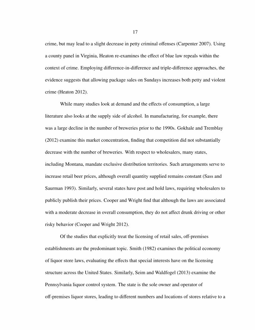
17
crime, but may lead to a slight decrease in petty criminal offenses (Carpenter 2007). Using
a county panel in Virginia, Heaton re-examines the effect of blue law repeals within the
context of crime. Employing difference-in-difference and triple-difference approaches, the
evidence suggests that allowing package sales on Sundays increases both petty and violent
crime (Heaton 2012).
While many studies look at demand and the effects of consumption, a large
literature also looks at the supply side of alcohol. In manufacturing, for example, there
was a large decline in the number of breweries prior to the 1990s. Gokhale and Tremblay
(2012) examine this market concentration, finding that competition did not substantially
decrease with the number of breweries. With respect to wholesalers, many states,
including Montana, mandate exclusive distribution territories. Such arrangements serve to
increase retail beer prices, although overall quantity supplied remains constant (Sass and
Saurman 1993). Similarly, several states have post and hold laws, requiring wholesalers to
publicly publish their prices. Cooper and Wright find that although the laws are associated
with a moderate decrease in overall consumption, they do not affect drunk driving or other
risky behavior (Cooper and Wright 2012).
Of the studies that explicitly treat the licensing of retail sales, off-premises
establishments are the predominant topic. Smith (1982) examines the political economy
of liquor store laws, evaluating the effects that special interests have on the licensing
structure across the United States. Similarly, Seim and Waldfogel (2013) examine the
Pennsylvania liquor control system. The state is the sole owner and operator of
off-premises liquor stores, leading to different numbers and locations of stores relative to a
18
license-to-operate system. While Toma (1988) examines retail license quotas, the analysis
is limited to the context of dry/wet counties—states with more restrictive licensing appear
to have higher numbers of dry counties.
Within the economics of alcohol literature, there is a contribution to be made by
examining how the market prices tradable retail licenses. Broadly speaking, relatively
little has been done examining on-premises retailers. More specifically, no literature exists
looking at license prices in the context of quotas. This topic also has relatively wide
applicability, as almost half of states allow transfers of retail licenses (although not all
have license quotas).20
Supporting Literature
While the issue of tradable alcohol retail licenses remains untreated in the
economics of alcohol, the topic of tradable permits is pertinent in other several other areas
of economics. Several other areas in economics have well developed literatures on the
trading and pricing of permits and production quotas, informing how the issue of alcohol
licenses may be approached.
In the field of environmental and resource economics, the literature on tradable
permits has existed since the 1960s. Crocker (1966) and Dales (1968) describe systems to
govern pollution of air and water, respectively, using markets for pollution rights.
Establishing tradable pollution permits may be a more efficient management mechanism
to reduce the negative externalities of emissions than direct regulation or a tax/subsidy
20Just over twenty states permit the transfer of retail licenses. This figure was compiled examining all fiftystates’ online statutes individually.

19
system, as the market is more responsive to emitter/receptor preferences (Crocker 1966).
Similarly, by employing a market system rather than charging producers directly for water
rights, regulators are relieved of the need to establish the price level necessary to achieve
the desired reduction in pollution (Dales 1968). The work of both Crocker and Dales is
widely applicable, serving as the foundation for a broad literature on tradable pollution
rights.
Similarly, tradable production permits are used with relative frequency in
agriculture. For example, the United States has employed both tobacco and peanut
production quotas (Rucker et al. 1995). The federal quota system for tobacco, in
particular, is similar in certain respects to the Montana alcoholic beverage license quota
system. Tobacco quota may be transferred by producers within counties, but cannot cross
county lines—alcohol retail licenses face similar transfer restrictions. Such limitations
create divergent prices (quota lease rates and sale values) between areas, with potential
gains from allowing trade. That said, Leasers of high price quota would be less well off
financially, while lessees would be better off financially (Rucker et al. 1995).
Another license market exhibiting similar characteristics to the Montana alcohol
licensing system is the famous example of taxicab medallions in New York City. The city
requires taxis to possess a medallion to operate, limiting the number of taxicabs in use.
Medallions are freely tradable, frequently fetching prices upwards of $ 1 million (NYC
Taxi & Limousine Commission 2013). Like alcohol retail licenses, possession of a
medallion confers the right to operate, but does not directly limit output. This system is
distinct from pollution and agricultural quotas, which strictly limit production. While the

20
imposition of the quota confers monopoly rents on those who were currently operating,
entrants into the market face normal profits as the medallion price rises to dissipate profit
(Tullock 1975). The existence of a positive price for medallions, however, does not
necessarily imply an inefficient outcome. For example, the barrier to entry may reduce
externalities associated with congestion. It may also secure a premium for honest
drivers—licensing may tend to push up quality in taxi services (Demsetz 1982, Cairns and
Liston-Heyes 1996).
Also related is the literature on big-game hunting permits. Several western states
allocate hunting permits via lottery, the same process by which Montana issues new
alcohol retail licenses. The Colorado permit lotteries, moreover, are preferential, not
unlike the issuance of RBW licenses (Buschena et al. 2001). Unlike the alcohol licenses,
the hunting permit lotteries occur on an annual basis. While the states frequently distribute
non-transferable hunting licenses annually, alcohol retail licenses are issued once, then
may be subsequently traded on the open market. While this limits the implications of this
literature for alcohol licensing, several underlying characteristics of the two systems
remain the same. People will tend to enter lotteries, for example, until the cost of entering
equals the expected value (Nickerson 1990, Scrogin et al. 2000, Buschena et al. 2001).
Similarly, restrictions on licenses (e.g., antlerless hunt permits or gaming restricted liquor
licenses) will unequivocally have non-positive effects on demand (Nickerson 1990). This
last point is directly applicable to the license system in Montana, which allows different
activities based on license type.
While there does not exist a specific literature regarding the issuance and trade of

21
alcohol retail licenses, other areas may provide insight into developing tools for analysis.
The topics of agricultural production quotas and taxicab medallions have particular
relevance for Montana’s licensing system, given the tradable nature of the quota. Even so,
relatively little has been done in terms of determining how transferable operational
licenses are priced. Coupled with the lack of work in the area of alcoholic beverage
retailers, again, a clear contribution to the literature is possible.
22
THEORY
The Competitive Market Model
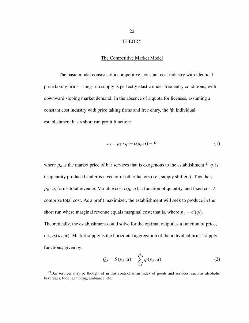
The basic model consists of a competitive, constant cost industry with identical
price taking firms—long-run supply is perfectly elastic under free-entry conditions, with
downward sloping market demand. In the absence of a quota for licenses, assuming a
constant cost industry with price taking firms and free entry, the ith individual
establishment has a short run profit function:
πi = pB · qi − c(qi,α) − F (1)
where pB is the market price of bar services that is exogenous to the establishment.21 qi is
its quantity produced and α is a vector of other factors (i.e., supply shifters). Together,
pB · qi forms total revenue. Variable cost c(qi,α), a function of quantity, and fixed cost F
comprise total cost. As a profit maximizer, the establishment will seek to produce in the
short run where marginal revenue equals marginal cost; that is, where pB = c′(qi).
Theoretically, the establishment could solve for the optimal output as a function of price,
i.e., qi(pB,α). Market supply is the horizontal aggregation of the individual firms’ supply
functions, given by:
QS = S (pB,α) =
k∑i=1
qi(pB,α) (2)
21Bar services may be thought of in this context as an index of goods and services, such as alcoholicbeverages, food, gambling, ambiance, etc.

23
where k is the total number of competing establishments. For the purposes of the model,
short run supply is assumed to have an upward slope.
In a competitive industry model, profit and loss determine the long-run number of
firms operating in the market. If price is above an establishment’s average cost, it earns
positive profit. In figure 1, case 1 presents the profit-earning case graphically, with the
shaded area denoting economic profit. If existing establishments are earning profit,
additional businesses will enter, shifting market supply out. As a result, price declines and
economic profits decrease. Conversely, if price is below an establishment’s average cost,
the business experiences negative profit (loss), denoted by the shaded area in case 2.
Economic loss causes establishments to exit, reducing market supply and increasing price,
causing profits to increase. If price equals average cost, there is no profit, illustrated in
case 3. When economic profit is equal to zero, there will be neither entry nor exit in the
market. Given entry or exit, market supply shifts until price equals average cost, as in case
3. All else equal, the long run market supply is perfectly elastic, as firms enter or exit until
profit equals zero.
Consequently, market demand sets the long run equilibrium quantity. Market
quantity demanded is given by the function:
QD = D(pB,β) (3)
where β is a vector of factors that affect demand (i.e., demand shifters). By setting the
long run equilibrium quantity, market demand determines the long run number of

24
establishments as well. Thus, the long run number of establishments in the market, k∗, is a
function of market price, with zero profit for each establishment in equilibrium.
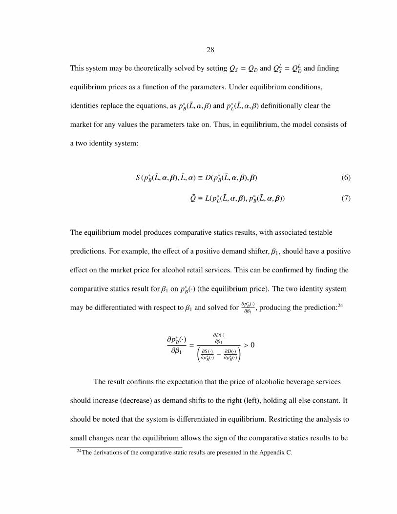
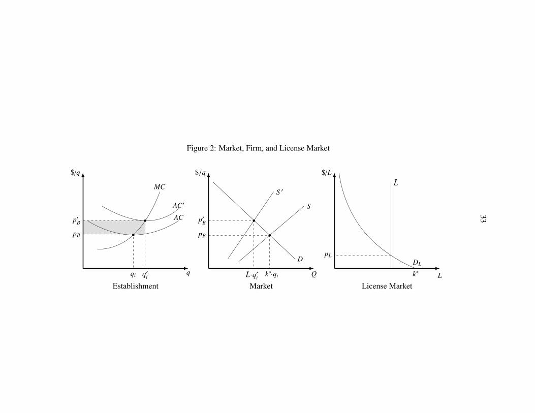
Quota for Licenses
The introduction of a binding license quota to the model limits the number of
establishments to fewer than would exist under free entry. Because fewer establishments
operate under the license system, supply shifts back and becomes less elastic relative to
the free entry scenario. In figure 2, S and S ′ denote the short-run market supplies for the
free entry and license quota scenarios, respectively. Supply under the license quota, S ′,
does not become perfectly inelastic. The quota is on the number of establishments, rather
than on output directly. Establishments may still adjust along other margins to increase
quantity (e.g., they may increase available seating). The reduction in supply causes an
increase in the equilibrium price, from pB to p′B, which would create profit in the short run
(the shaded area in figure 2). If the licenses are tradable, however, this profit does not
persist. Rather, a market forms for the licenses. In addition, Long run supply is no longer
perfectly elastic with the addition of a quota. New firms cannot freely enter to bid down
profit.
In the market for licenses, supply is perfectly inelastic, set exogenously by a
regulatory agency. Thus, quantity supplied is given by the function:
QLS = L (4)
25
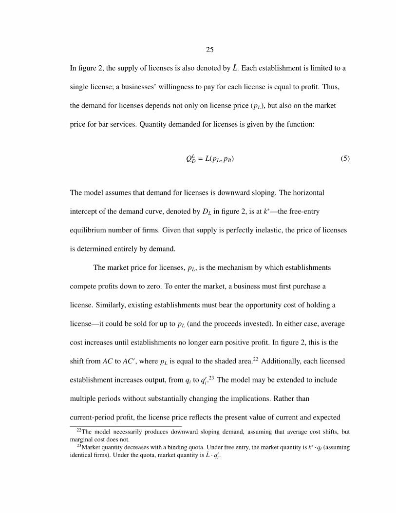
In figure 2, the supply of licenses is also denoted by L. Each establishment is limited to a
single license; a businesses’ willingness to pay for each license is equal to profit. Thus,
the demand for licenses depends not only on license price (pL), but also on the market
price for bar services. Quantity demanded for licenses is given by the function:
QLD = L(pL, pB) (5)
The model assumes that demand for licenses is downward sloping. The horizontal
intercept of the demand curve, denoted by DL in figure 2, is at k∗—the free-entry
equilibrium number of firms. Given that supply is perfectly inelastic, the price of licenses
is determined entirely by demand.
The market price for licenses, pL, is the mechanism by which establishments
compete profits down to zero. To enter the market, a business must first purchase a
license. Similarly, existing establishments must bear the opportunity cost of holding a
license—it could be sold for up to pL (and the proceeds invested). In either case, average
cost increases until establishments no longer earn positive profit. In figure 2, this is the
shift from AC to AC′, where pL is equal to the shaded area.22 Additionally, each licensed
establishment increases output, from qi to q′i .23 The model may be extended to include
multiple periods without substantially changing the implications. Rather than
current-period profit, the license price reflects the present value of current and expected
22The model necessarily produces downward sloping demand, assuming that average cost shifts, butmarginal cost does not.
23Market quantity decreases with a binding quota. Under free entry, the market quantity is k∗ ·qi (assumingidentical firms). Under the quota, market quantity is L · q′i .
26
future profits.
Additionally, profit (or expected profit) may differ based on license attributes. In
the context of Montana’s licensing system, there are several tiers of licenses.
All-beverage, beer and wine, and RBW licenses may be thought of as having distinct
markets, each following the model above. The licenses are imperfect substitutes, with
premiums for certain license types. An all-beverage license should yield a higher expected
profit than a beer and wine or RBW license, as it permits the largest scope of services.
Similarly, a license that allows gambling should sell for a higher price than a
gaming-restricted license, all else equal.
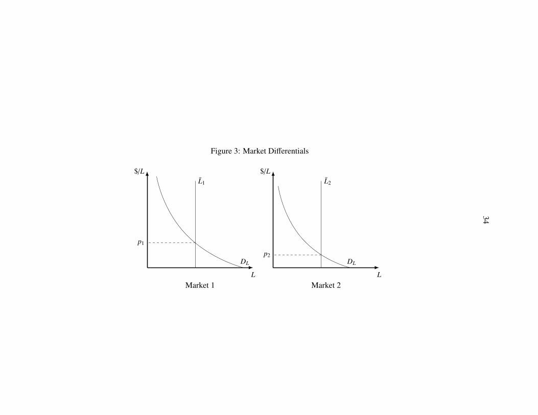
Market Differentials
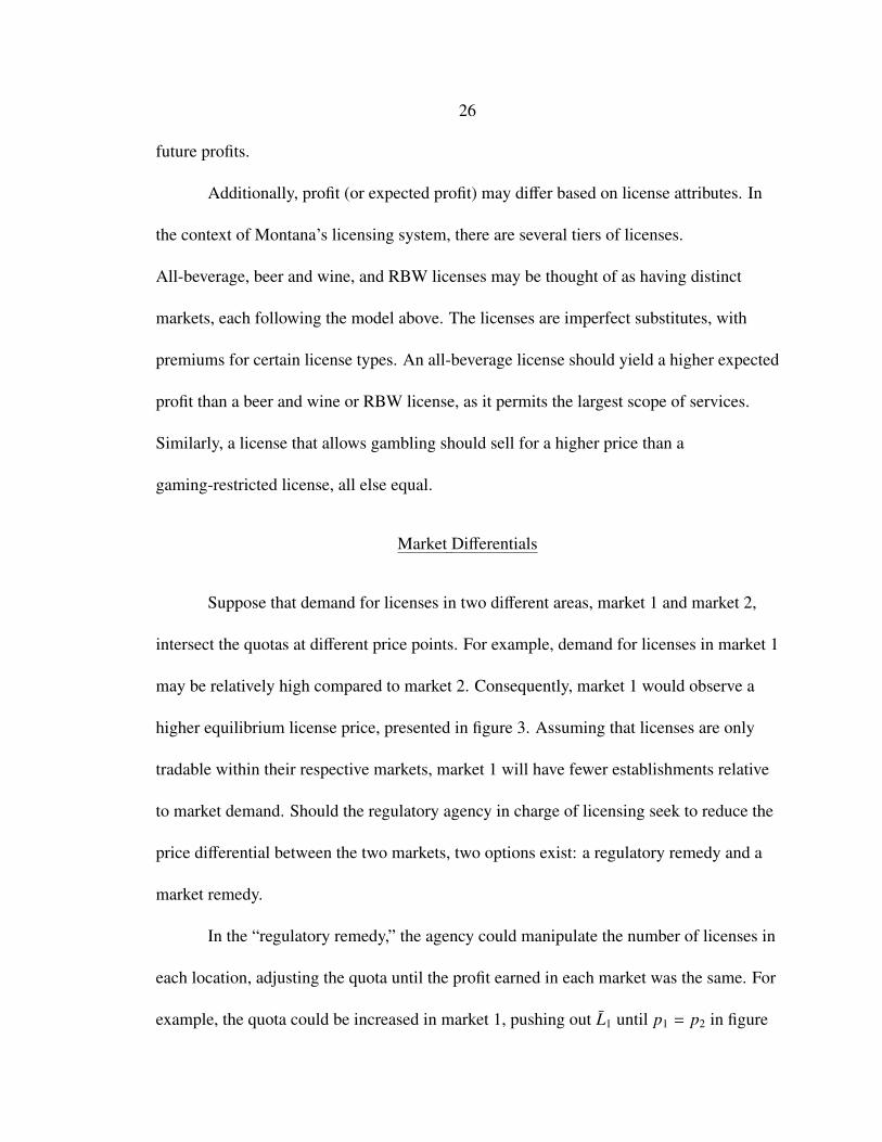
Suppose that demand for licenses in two different areas, market 1 and market 2,
intersect the quotas at different price points. For example, demand for licenses in market 1
may be relatively high compared to market 2. Consequently, market 1 would observe a
higher equilibrium license price, presented in figure 3. Assuming that licenses are only
tradable within their respective markets, market 1 will have fewer establishments relative
to market demand. Should the regulatory agency in charge of licensing seek to reduce the
price differential between the two markets, two options exist: a regulatory remedy and a
market remedy.
In the “regulatory remedy,” the agency could manipulate the number of licenses in
each location, adjusting the quota until the profit earned in each market was the same. For
example, the quota could be increased in market 1, pushing out L1 until p1 = p2 in figure

27
3. Similarly, the quota could be reduced in market 2 to reduce the price differential. In
either case, the adjustment of the quota and subsequent license price effects would lead to
similar licensing costs between markets.
In the “market remedy,” rather than directly increasing or decreasing the number
of licenses in each market, the regulatory agency could allow trades between the markets.
In this case, establishments wishing to enter market 1 could purchase licenses from market
2. As a result, licenses issued would increase in market 1 and decrease in market 2, as
licenses floated between areas. In the absence of transaction costs, the licenses will be
reallocated across markets until p1 = p2. Again, the reduction in the price differential
would lead to similar licensing costs between markets. In addition, allowing trade would
maximize social net benefits from the total number of licenses (L1 + L2) across the two
markets .
Application of the Model
Using the competitive market model with a binding quota, several testable
implications arise. Consider the four equation system, comprised of equations 2-5. These
include quantities supplied and demanded for alcohol retail services (QS and QD), and
quantity supplied and demanded of licenses (QLS and QL
D):
QS = S (pB, L,α) QLD = L(pL, pB)
QD = D(pB,β) QLS = L
28
This system may be theoretically solved by setting QS = QD and QLS = QL
D and finding
equilibrium prices as a function of the parameters. Under equilibrium conditions,
identities replace the equations, as p∗B(L, α, β) and p∗L(L, α, β) definitionally clear the
market for any values the parameters take on. Thus, in equilibrium, the model consists of
a two identity system:
S (p∗B(L,α,β), L,α) ≡ D(p∗B(L,α,β),β) (6)
Q ≡ L(p∗L(L,α,β), p∗B(L,α,β)) (7)
The equilibrium model produces comparative statics results, with associated testable
predictions. For example, the effect of a positive demand shifter, β1, should have a positive
effect on the market price for alcohol retail services. This can be confirmed by finding the
comparative statics result for β1 on p∗B(·) (the equilibrium price). The two identity system
may be differentiated with respect to β1 and solved for ∂p∗B(·)∂β1
, producing the prediction:24
∂p∗B(·)∂β1
=
∂D(·)∂β1(
∂S (·)∂p∗B(·) −
∂D(·)∂p∗B(·)
) > 0
The result confirms the expectation that the price of alcoholic beverage services
should increase (decrease) as demand shifts to the right (left), holding all else constant. It
should be noted that the system is differentiated in equilibrium. Restricting the analysis to
small changes near the equilibrium allows the sign of the comparative statics results to be
24The derivations of the comparative static results are presented in the Appendix C.

29
determined with relative ease. Thus, the derivative of p∗B(·) is taken (with respect to β1).
The prediction is local, only applying to values near the equilibrium price.
A more interesting effect is that an increase in β1 should have a positive effect on
the price for a license, p∗L(·). This prediction is perhaps less intuitive than the previous
result, as β1 relates only indirectly to the market for quota. Nonetheless, the model
produces a comparative statics results that supports this expectation. Again, the two
identity system may be differentiated with respect to β1, but solved for ∂p∗L(·)∂β1
. This process
produces the testable implication:
∂p∗L(·)∂β1
=−∂D(·)∂β1·∂L(·)∂p∗B(·)(
∂S (·)∂p∗B(·) −
∂D(·)∂p∗B(·)
)·∂L(·)∂p∗L(·)
> 0
Thus, the price of licenses should increase (decrease) as the demand for alcohol
retail services increases (decreases) as well. Factors such as student population and
tourism should all positively influence the price of alcoholic beverage licenses for a given
quota level. Conversely, the restriction of gambling rights placed on certain licenses, or
shrinking population in a quota market should depress prices in the license market.
Similarly, the model produces testable predictions regarding changes in the
quantity of licenses available under the quota. The comparative statics result for L on
price in the market for alcohol retail services is:
∂p∗B(·)∂L
=
∂S (·)∂L(
∂D(·)∂p∗B(·) −
∂S (·)∂p∗B(·)
) < 0

30
The result implies that the price of services should decrease (increase) as the quota
increases (decreases). Again, the result is fairly intuitive, given how the assumptions of
the model. An increase in quota will increase market supply, leading to a lower prices for
bar services. Another more interesting testable implication arises for the effect of L on the
price of licenses. Differentiating they system with respect to L and solving for ∂p∗L(·)∂L
produces the result:
∂p∗L(·)∂L
=
(∂D(·)∂p∗B(·) −
∂S (·)∂p∗B(·)
)−
∂L(·)∂p∗B(·) ·
∂S (·)∂L(
∂D(·)∂p∗B(·) −
∂S (·)∂p∗B(·)
)·∂L(·)∂p∗L(·)
< 0
For an increase (decrease) in the quantity of available licenses, the price of licenses will
decrease (increase). This straightforward result has implications for both the regulatory
and market remedy for divergent prices above. For example, releasing additional RBW
licenses in 2007 should cause the price of such licenses should decrease.
Under limited circumstances, establishment owners may transfer floater licenses
between quota areas. The buyer’s area should observe lower prices as the number of
licenses in circulation increases, while the seller’s area should observe the opposite effect.
Given the limited conditions under which such trades occur, however, the effects of floater
licenses moving between areas tends to be quite small. Adding one additional license to
the 98 all-beverage licenses currently in Billings only constitutes a 1.02 percent increase.
As a result, the prediction is unlikely to be supported empirically in such conditions.
A caveat to the license price predictions is that they only apply to cases where the
quota for licenses is binding. If an area is under quota, the free-entry number of firms
operate in the market. In figure 2, this scenario would occur if L were in excess of k∗.

31
There would be no economic profit, leading to a zero-price for licenses. Marginal changes
in license demand or quota would not cause license prices to change. A marginal change
could conceivably cause L to become equal to k∗, but price would remain zero. Thus, the
predicted effects regarding p∗L(·) above should be zero in non-binding areas.

32
Figure 1: Positive, Negative, and Zero Proft
p1
q1
AC
MC
Q
Case 1: Profit
$/Q
p2
q2
AC
MC
Q
Case 2: Loss
$/Q
Q
Case 3: Zero Profit
$/Q
AC
MC
p3
q3
33
Figure 2: Market, Firm, and License Market
AC
MC
AC′
pB
qi
p′B
q′i q
Establishment
$/q
Q
Market
$/q
D
S
S ′
pB
k∗·qi
p′B
L·q′i LLicense Market
$/LL
DL
k∗
pL
34
Figure 3: Market Differentials
LMarket 1
$/LL1
DL
p1
LMarket 2
$/LL2
DL
p2

35
DATA AND METHODOLOGY
Data
The Montana Department of Revenue must approve all transfers of alcohol
licenses. As part of the approval process, the department records data on all transfers,
including the sale price, buyer’s quota area, transaction type, application date, and
approval date. Transaction types include transfer of ownership (sale of a license with the
establishment), transfer of ownership and location (sale of a license to a new
establishment), transfer of location (no sale, but a relocation of the establishment), new
issuance, and corporate structure change (a term that includes business decisions ranging
from restructuring where no money changes hands to sales of a partial financial interest in
a license). The information is public record, published on the department’s website with
transactions from 2006-2013. Additionally, earlier price data from 2002-2007 are
available, also obtained from the Department of Revenue.25
The two data sets partially overlap for 2006-2007. In total, there are 1,227
observed transactions forming pooled cross-sections over time. Included in the data are
781 all-beverage, 234 beer retail, and 157 restaurant beer and wine transactions.26 Further,
the data contain only 48 transactions involving the major license types prior to 2005 (the
file was not completed for 2002-2004), all of which are dropped. Similarly, other data
used in the analysis, including census estimates and tax revenue numbers, are not yet
25These data were obtained prior to the new computer system implemented by the department in 2007, andare now unavailable.
26The infrequency of the other license types precludes analysis. Only seven observations across all otherlicense types involved trades between private parties.
36
available for 2013, causing the most recent year’s data to be dropped (50 observations).
New issuances do not involve market prices. Rather, the department collects a
fixed initial licensing fee based on a schedule.27. Similarly, transfers of location do not
involve changes in the ownership of a license or an exchange of money.28 In the case of a
death of a licensee, the ownership of the license may revert to the estate, or to whomever
has financial control over the estate. These transactions do not involve market prices, and
have been omitted from the analysis.
Several low-price observations are also dropped from the data set. Observations
listing a price of zero are omitted, with all such transactions coming from the 2002-2007
data. This change makes the earlier and later data more consistent, as the department does
not include any zero-price transactions in their data post-2007. Similarly, several very
low-priced transactions from 2007-2013 are dropped. Selling a license for $1.00-10.00
(well below annual licensing fees) when licenses trade routinely for six-figure values, is
indicative of some unobservable characteristic in the data (e.g., a father selling a license to
son). As a result, these observations are dropped. Finally, six inconsistent observations are
omitted. The transactions appear to be duplicates, either across space (i.e., listed in both
Missoula and Petroleum counties) or time (i.e., the same information with overlapping
dates). With the inconsistent observations, the information from the newer data set is used
in place of the older data. Table 1 illustrates the breakdown of the number of observations
27Initial licensing fees may be found in M.C.A. 16-4-420 and 16-4-501.28As a result, transfers of location should list a price of zero. In the data, however, several transactions
recorded as transfers of location list non-zero prices. To identify which transactions are mislabeled, allobservations flagged as a transfer of location listing a price of over $800.00 are changed to ”transfer ofownership and location.” Several transfers of location appear to list the annual licensing fee as the price; $800is the highest annual fee, serving as the line of demarcation.

37
and those that are omitted.
Further observations have potential clerical errors, either between or within each
data set. For each type of potential problem, the observation is flagged with a binary
variable. The most commonly flagged issue is for a missing transaction type, with 71
occurrences.29 Further, all observations missing an application date fall into this category,
with 53 observations in 2006. As a result, these observations cannot be treated as random.
The application date for each is imputed using the mean time between application and
approval, and a dummy variable is included for regressions. In effect, “missing” is treated
as a distinct transaction type.
Between 2005 and 2012, 52 of the 56 counties in Montana observe at least one
transaction, with the six most populous counties (Yellowstone, Missoula, Flathead,
Gallatin, Cascade, Lewis & Clark) observing the the greatest number of transactions.
Table 2 reports the the total number of transfers of ownership across every county in
Montana for 2005-2012.
Just as the largest counties have the most transactions, the largest cities in Montana
observe more trades than the smaller areas. In addition, they tend to observe higher prices,
with Billings, Missoula, and Bozeman each observing a maximum price of $1,000,000
(nominal) for an all-beverage license. For transfers of ownership and transfers of
ownership and location, the average prices of all-beverage licenses (excluding floaters) by
29Other potential errors include incomplete entries from 2002-2007; inconsistent dates and/or prices be-tween data sets; observations that appeared in the 2007-2013 data in Aug. 2013 but not Feb. 2014, orvice-versa; unusually long times between application and approval; and mismatches of license type. In allcases, if an observation appears in both data sets, the newer value supersedes the older. A binary variable foreach potential error was initially included in the regressions. They were insignificant, however, and are notincluded in the results section.

38
year in the 15 largest cities in Montana are reported in table 3. Floaters are excluded, as
the licenses are purchased from a low-price area but reported in the buyer’s quota area.
Buyers act as monopsonists–the purchase prices should tend to reflect the market
conditions in the seller’s location, which is not identified in the data. Not every major city
records a transaction for each license type every year, and those that do may have low
numbers of trades. Bozeman, for example, records approximately two transfers of
ownership or transfers of ownership and location of all-beverage licenses each year,
making the mean price susceptible to outliers (e.g., the dramatic dip in price in 2010). The
markets for all-beverage licenses may be the deepest, but the usable license price data
covers all transfer types across the three major license classes.
In evaluating the determinants of license price, economic characteristics of each
quota area are important controls to include, as they should affect the derived demand for
alcohol retail licenses. Provided that the goods and services licensed establishments offer
are normal, higher incomes will shift demand for alcohol out and increase license values,
all else equal. Conversely, the effect of unemployment is unclear—higher unemployment
could cause license prices to move in either direction.30 Median household incomes,
reported at the county level, are obtained from the U.S. Census Bureau’s Small Area
Income and Poverty Estimates. Unemployment, also reported at the county level, are from
the U.S. Bureau of Labor Statistics. Table 4 reports the median household incomes in the
15 largest counties and Montana overall for 2005-2012.31 Table 5 does the same for
30The short run effect can be positive or negative. In the long run, lower incomes should decrease con-sumption (lowering license values).
312012 is the most recent available data.

39
unemployment.
Another important factor for both supply and demand for licenses is population.
The U.S. Census Bureau provides annual city-level population estimates for all
incorporated communities, along with the unincorporated county balance (the population
of a county, less the population residing in incorporated areas). Population growth may
also be important, as state law sets quotas based on current population, but proprietors
value licenses based on expected future income. While positive growth may have a limited
effect (licensees probably anticipate the state issuing more licenses), negative growth
should decrease license prices (the state does not take licenses away if population shrinks).
Population level may serve as a better control than growth, however, as a 1 percent growth
rate in Billings is fundamentally different than 1 percent growth in Broadview. In Billings,
1 percent growth is about half of what is necessary to increase the quota by an additional
license; Broadview would require a much higher growth rate to secure a larger quota.
Table 6 reports the population growth rates for the 15 largest towns in Montana.
Immediately apparent are the drops in the population growth rate in the some of the
previously fastest growing cities. Belgrade, Bozeman, and Kalispell each witnessed large
drops in growth in 2009-2010, with Belgrade’s changing sign in 2009. Similarly, the
growth rates in Livingston and Whitefish, while smaller in the preceding years, also turn
negative in 2009-2010. In contrast, Billings and Helena maintain consistent growth over
the timeframe. Another interesting phenomena to note is that Anaconda and Butte, while
having reputations as shrinking communities, tend to have growth around zero. Given
there is no consistent shrinking population, the growth rate will probably not affect license
40
prices over the time frame of this study.32
Along with population, demographic makeup may also serve as important
controls. The U.S. Census Bureau produces age, gender, racial, and ethnic population
estimates at the county level. Of these measures, the age brackets, reported in five-year
intervals, may be the most interesting. The proportion of an area’s population between the
ages of 20-44, for example, may tend to have a positive effect on demand. The variation in
the demographic information, however, is quite low. While there are differences across
counties, there is very little change across time.
University population and the rate of tourism will tend to have a positive effect on
demand for bar services, all else equal. The licensing system bases communities’ quotas
on permanent population, not taking into account students, visitors, or tourists. As a
result, cities that have a large university population relative to permanent population
should see higher derived demand for licenses, with correspondingly higher prices. The
National Center for Education Statistics provides annual fall enrollments for all two and
four year institutions in Montana, through the Integrated Postsecondary Education Data
System (IPEDS). These data include numbers for public, private, and tribal institutions.
Table 7 reports enrollment for each quota area with a school.33
Unfortunately, the number of visitors and tourists to any particular community in a
given year is not generally available. Instead, the Montana hotel and lodging tax may
32Again, positive growth should have little impact on prices, while negative growth should push pricesdown.
33Although the different types of universities may be expected to have different impacts, they are treatedthe same in the analysis. The results are robust to separating enrollment by type (e.g., private/public/tribal, ortwo-year/four-year.

41
serve as a proxy. Collected by the Department of Revenue, the lodging tax consists of a
flat 4 percent on rent charged for rooms, plus a 3 percent sales tax (for a total tax of 7
percent). The tax is not an exact measure of the number of guests, as the reported revenue
is subject to differences in room rates. The supply of hotel rooms, however, will probably
tend to be quite inelastic over any relatively short period of time. As a result, demand
should drive most of the changes in revenue within a given county.
The Department of Revenue reports the lodging tax at a county level, with several
smaller counties reported jointly.34 To impute county-level revenue numbers for the few
jointly reported counties, the total revenue is divided based on the number of hotels in
each county (e.g., if there are four hotels across two counties, one in the first and three in
the second, the first county would have 25 percent of the total reported revenue imputed as
the county-level number).35 Table 8 reports annual lodging tax revenue, for the 15 largest
counties in Montana.
Immediately apparent is the relationship between the hotel tax revenue and the
mean license prices in table 3. Gallatin, Yellowstone, Missoula, and Flathead counties
tend to have the highest average license prices (and the most transactions). Similarly, the
tax revenue produced by the hotel industry in each town is far above the other larger
counties. In addition to being potential tourist destinations, the presence of the two largest
Montana universities in Bozeman and Missoula probably boost the lodging tax revenues
for their respective counties.
34Counties whose lodging tax revenues were aggregated to protect proprietors privacy includeCarter/Golden Valley/Treasure, Prairie/Wibaux, Garfield/McCone, and Judith Basin/Liberty/Petroleum.
35How the data is imputed does not influence the results. The jointly reported areas log very few transac-tions, all with very low prices.

42
An important facet of Montana’s alcohol licensing system is the packaging of
gambling rights with all-beverage and beer retail licenses. In addition to gambling license
fees, the Montana Department of Justice collects a 15-percent income tax on net revenues
from gambling machines (the money fed into the machines less the money paid out in
winnings). The department reports the tax revenue, along with the number of licensed
establishments and the number of video gaming machines. For the earlier biennial reports
(pre-2007), the Department of Justice reports numbers for all incorporated communities,
along with numbers for the county balance. In later reports (post-2007), the department
begins reporting at the county-level, along with several major cities.
To impute city-level revenue for the post-2007 data, the historical average split
from the pre-2007 data are used. For example, the Gallatin County total revenue, less
Bozeman and Belgrade, is divided between Manhattan, Three Forks, West Yellowstone,
and the county balance. The average proportion of the revenue attributed to each area
from 2001-2006 (once Bozeman and Belgrade have been subtracted from the county total)
is used to impute revenue numbers for each of the smaller communities. The same process
is used for each county in Montana. Table 9 reports video gambling tax revenue for major
cities, by year.
The supply of licenses in a quota area is perfectly inelastic for any given year, set
by the formula using population laid out in state law. The Department of Revenue updates
the quotas annually, using the previous year’s city-level population estimates from the
U.S. Census Bureau. Measures of quota and the number of issued licenses are currently
available from the department for all-beverage, beer retail, and restaurant beer and wine
43
for 2008-2013, along with an existing report from 2005.36 For 2006 and 2007, updated
city-level population estimates from the U.S. Census Bureau are used to impute quotas.37
Similarly, the number of licenses issued for 2006 and 2007 are interpolated using
the 2005 and 2008 quota reports. The interpolated number of all-beverage and beer and
wine licenses issued in 2006 is one-third the difference between 2008 and 2005, added to
the 2005 issued licenses; 2007 values are assigned using the 2008 numbers less one-third
the difference. Both values are rounded to the nearest whole number. For RBW licenses,
the 2006 licenses issued take on the 2005 value, while the 2007 interpolated number is the
average of 2005 and 2008. The functions differ, as the RBW quota doubles in 2007 due to
a legislative change in the quota formula. A confounding factor is the merging of
Bozeman and Belgrade in 2006. Prior to 2006, the town’s respective quota areas did not
overlap. In 2006, however, it was determined that the city limits for each town were within
10 miles of each other. Tables 10-12 gives the quota and licenses issued for all-beverage,
beer retail, and RBW licenses in the 15 largest cities.
Each of the largest towns are all significantly over quota. All except Billings,
moreover, exceed 143 percent of quota, meaning that they are not eligible to float in
additional licenses. While the towns listed above are well over their quotas, they are hardly
exceptional. Indeed, much of the state has more licenses issued than technically allowed
by the quota. Several areas with the greatest surplus of licenses are Butte, Anaconda, and
Red Lodge, each of which is over quota by more than 300 percent. For 2012, Butte and
36The 2005 quota spreadsheet was obtained before the update to the Department of Revenue’s computersystem in 2007; it is no longer available from the department.
37These imputed quotas will not be perfect replicas the original (unavailable) quota spreadsheets. Thedepartment uses initial estimates, which the Census Bureau subsequently updates.

44
the surrounding county (Silver Bow) are alloted 25 licenses, with 86 total licenses in use;
Anaconda (and Deer Lodge County) stands at 9 and 30; Red Lodge, 4 and 16. Overall,
119 of the 176 quota areas are at or above their respective quotas for 2005-2012.
While most incorporated communities are over quota, many counties are not.
Indeed, the unincorporated areas of the six most populous counties in Montana are tend to
be under quota, ranging from 11 under (Cascade, Lewis and Clark) to 32 under
(Yellowstone) as of 2012. Collectively, however, the Department of Revenue has issued
more total licenses statewide than the official quota as set by state law, with 81 of the 176
distinct areas over quota.38
Collectively, 758 observations are from areas that are at or above their all-beverage
license quotas. Of the 134 observations from non-binding areas, 95 are from areas more
than one license below their quota. These tend to be from the unincorporated areas in the
larger counties, mentioned above. 39 observations are from areas that are technically
non-binding, but are short of meeting their quota by one license. Further, of those 39, 28
are from areas that have binding quotas for at least one year between 2005-2012. These
observations are interesting in that the associated license prices look more like the prices
from binding areas than non-binding (the prices in non-binding areas should be near zero).
It is possible that entrants into the almost-binding markets would rather purchase a license
an existing license than apply for a new one. If the prices are relatively low, buying a
license may be worth avoiding an additional competitor. Unfortunately, the relative lack of
observations in these markets precludes statistical analysis on the topic.
38The difference between the total number of operational licenses in the state and the sum of the quotasacross all areas is +271 for 2012.

45
Unlike the all-beverage licenses, the other two on-premises license types, beer and
wine retail and restaurant beer and wine, do not systematically exceed their respective
quotas. As of 2012, only 15 of the 176 quota areas have beer and wine licenses in excess
of quota, with only Butte and Whitefish exceeding quota by more than 2 licenses.
Similarly, only two areas consistently exceed the RBW license quota—Whitefish and
Kalispell. Collectively, the department has issued fewer total beer retail and RBW licenses
than quota would permit across the state. One phenomenon to note about RBW licenses is
the relatively slow adjustment. With the doubling of the RBW quotas in 2007, even the
highest-price markets take several years to bring the additional licenses into use.
Additional variables of potential interest include the number of small breweries
and domestic distilleries in a quota area. Both types of manufacturers may operate
on-premises establishments, acting as substitutes for establishments with a retail license.
A list of breweries and their years of operation was compiled using Montana Beer:
A Guide to Breweries in Big Sky Country, complemented using breweries’ commercial
websites. Unfortunately, there is quite limited variation across the span of the data, with
the majority of growth occurring at the very end of the panel. Similarly, the Montana
Department of Agriculture lists only four domestic distilleries, with the oldest beginning
operations in 2009 (Harrison, 2011). As such, variables for the number of small breweries
and domestic distilleries have been omitted.
Although the time frame of the data is relatively short, prices are deflated to be
directly comparable. The Producer Price Index (PPI) for Beer, Wine, and Liquor is used to
license prices in 2005 dollars. Similarly, the Mountain-Plains CPI is used to deflate

46
income, gambling revenue, and hotel revenue. Both indices are obtained from the Bureau
of Labor Statistics.
Figure 4 shows the distribution of license prices in 2005 dollars. The prices are
clearly clustered near zero (the first bin contains prices around $30,000 and under), with a
long tail to the right. Given how skewed the distribution is, it is probably preferable to
transform the data. Figure 5 illustrates the distribution after taking the natural log of
license price. Although the distribution of log prices still has a large number of
observations in each tail, the prices are clustered much more closely around the mean.
From the distributions, it appears that log license prices are preferable to levels.
Particularly, transforming the data reduces concerns of hetoerscedasticity and bias from
outliers.
To get a sense for the variation that drives the results, the variables may
summarized across the two different dimensions. Table 13 presents the means and
standard deviations of log license prices and the major right-hand side variable, by year
and for the entire data set. For ease of reporting and interpretation, the values for
gambling and hotel are reported as total revenues instead of tax revenues. Both are taxed
at constant rates: 15 percent for gambling, 7 percent for hotels. Thus, total revenue for
gambling is the reported tax revenue over 0.15; for hotels, it is reported tax revenue over
0.07. In addition, the revenues are reported in thousands for the sake of brevity.
The most notable features in table 13 are the dips in several variables in 2008. The
decrease in the mean is driven by where trades occur, however, not by an overall drop in

47
the variables.39 Otherwise, the means and standard deviations within year look to be fairly
consistent across time, and consistent with the values for the data as a whole.
Table 14 reports the means and standard deviations for the same variables, across
the 10 largest cities in Montana. As expected, the means for are much higher certain cities
than for the data set as whole. For example, Billings reports a mean gambling revenue
more than four times larger than the data set mean; Bozeman’s average hotel revenue is
more than than triple the data set mean. More striking is the discrepancies in the standard
deviations between the individual cities and the data overall. Excepting log license price,
the variation within cities (over time) is vastly smaller than across all variables. Indeed,
for many of the variables the standard deviations within city are routinely an order of
magnitude smaller.
Comparing the statistics in tables 13 and 14 help identify can where the variation
used to identify results is coming from. The means and standard deviations are far more
consistent when pooled by time than when pooled by city. Thus, finding measurable
effects are far more likely if regression rely on cross-sectional rather than on temporal
variation.
Empirical Methodology
To determine what factors affect how alcohol retail license prices are determined,
the basic econometric specification uses a log-level functional form. The dependent
variable is the natural log of license price, while the other right-hand side variables listed
39In 2008, Billings had fewer than half the trades it had in 2007.
48
above are measured in levels. As a result, the regression fits an exponential relationship
between the dependent and independent variables. Because the supply of licenses is
perfectly inelastic in each year, the most basic specification does not include any variable
for license supply. The quotas are subject to change across years, however, so alternative
specifications include controls for supply. Thus, the basic econometric specification takes
the form:
ln(Pricei jt) = β0 + β1Gambling jt + β2Hotel jt + β3Population jt + β4Age jt + β5Female jt
+β6Enrollment jt + β7Income jt + β8Unemployment jt + β9GamingRestrictedi jt
+LicenseTypei jtγ + TransactionTypei jtδ + εi jt
ln(Pricei jt) is the natural log of the license price for transaction i, in quota area j,
in year t. Gambling jt is total gambling revenue in the relevant quota area and year.
Similarly, Hotel jt is the total county-level hotel revenue attributed to quota area j in year
t.40 Population jt is the estimated population, while Age jt and Female jt are the proportion
of the population between 20 and 44 and the proportion that is female, respectively.
Enrollment jt measures university/college enrollment (taking on a value of zero for most of
the data), while Income jt and Unemployment jt control for quota-area and time economic
characteristics.
LicenseTypei jt is a vector of indicator variables for floater, beer and wine, and
RBW licenses.41 Similarly, TransactionTypei jt is a series of dummies for the transaction
40Again, the same hotel revenue is used for every observation in a county. For example, the 2005 hotelnumber from Gallatin County is used for both the Bozeman and Three Forks quota areas in 2005.
41For the purposes of the study, the ten resort all-beverage licenses in the data are included among the typ-

49
type: transfer of ownership, corporate structure change, or missing (transfer of ownership
and location is the omitted type).42 Finally, GamingRestrictedi jt is dummy variable that
takes a value of 1 if a beer and wine, floater, or all-beverage license does not have
gambling rights.
Across the different regressions, the specifications are first compiled without
supply variables, then add controls for license supply. With supply variables, the vector
QUOT A jt is included, specified in one of two ways. The first includes indicator variables
for binding beer retail and RBW quotas, along with percentage all-beverage quota and
percentage all-beverage quota squared. For the purposes of defining the dummy variable
for beer retail and RBW quotas, binding is defined as at or above quota.43 Unincorporated
quota areas have neither beer retail nor RBW quotas and take on a value of zero for each
indicator variable by default. A linear and quadratic term are included for percentage of
all-beverage quota, for a more flexible functional form.44 The second way the vector is
specified consists of the number of licenses issued for each of the three major license
types.
Because the regressions are specified in log-level form, the coefficients represent
ical all-beverage licenses. Although issued under different circumstances, resort all-beverage license pricesare not statistically distinguishable from all-beverage license prices. As such, the specifications do not dis-tinguish between the ten resort all-beverage and the other all-beverage licenses.
42The specifications do not include license/transaction type interactions, as there are not enough observa-tions for each combination for the interaction term to be meaningful (e.g., two or three observations for eachinteractive term). The results, however, are robust to their inclusion.
43A relatively small number of communities are above their beer retail quota. Areas appear to be abovequota for one of two reasons. First, several areas appear to have had historic decreases in population (e.g.,Butte and Anaconda). Second, the U.S. Census bureau may have over-estimated population in their initialintercensal estimates. If a population estimate is subsequently revised to a lower value, the relevant quotamay decrease.
44If a quota area is well below or well above their established quota, prices are expected to be low. Includinga quadratic term allows license values to peak. Unlike the other two license types, there is significant variationin percentage of quota.

50
percentage changes in price for a level change in the continuous right-hand side variables.
Coefficients on indicator variables, however, take on a slightly different interpretation, as
they are inherently discontinuous. If the dummy variable for a beer and wine retail license
takes on a value of one (with all-beverage as baseline), for example, the coefficient does
not represent the percentage difference in price compared to all-beverage licenses. Rather,
the coefficient must be transformed to produce an intuitive interpretation. The
transformation is relatively straight forward: supposing β is the estimated coefficient on a
dummy variable with ln(y) on the left hand side, the relative effect of the dummy taking a
value of 1 is
%4Y = 100 ·(eβ − 1
)This transformation provides the correct percent change in the dependent variable
(Halvorsen and Palmquist, 1980). It should be noted, however, that for coefficients with
magnitudes near zero, the reported values provide a close approximation.
The log-level functional form is employed initially for two reasons. First, the
distribution of log license prices avoids the long tail present in the distribution of level
license prices. The transformed data reduces potential bias from outliers, and reduces
concerns over heteroscedasticity. Second, the log-level regression produces the best fit out
of the different functional forms. The R-squared for the log-level is better than a log-log
model, making the former specification preferable. Comparing the log-level and the
level-level, however, is slightly more complicated.
Because the models employ different dependent variables, the sum of squared

51
residuals (and thus the goodness of fit) may not be used to compare the appropriateness of
the specifications directly. Rather, a Box-Cox transformation may be employed to scale
the variances, putting the sum of squared errors in the same units (Rao and Miller,
1971).45 Employing the transformation yields a sum of squared residuals (SSR) of 1,758
for the log-level model, compared to a SSR of 11,012 for the level-level. The difference in
the SSR between the log-level and the level-level model is significant at the 1 percent
level, indicating that the specifications with the log license prices is more appropriate.
In addition to the basic regression, three other sets of regressions are run as
robustness checks. In the first case, regressions are run on subsets of the data to look for
differential effects. Second, the basic regression is run employing two other functional
forms—specifically, level-level and log-log.46 Although the fundamental estimated
relationship between variables is different, significance should remain more or less the
same across the different functional forms. Finally, a set of results are produced
employing quota-area and year fixed effects, which is expected to condition out much of
the identifying variation.
The inclusion of fixed effects for year (but not quota-area) might also be
interesting. The variables for year could capture macroeconomics trends, without
conditioning out the cross-sectional variation of interest. The baseline results, however, do
not change in year fixed effects are included. In addition, the year dummy variables are
45The transformation consists of scaling the dependent variable. If the comparison consists of log andlevel dependent variables, the scaling factor is simply the inverse of the geometric mean. The results are thencompiled with the scaled left-hand side variable, for both specifications.
46Another potential specification is level-log. The results are similar, but somewhat less intuitive. Addi-tionally, it unequivocally provides the worst fit of all the different specifications. It is omitted for the sake ofbrevity.

52
not individually or jointly significant.47 Thus, time fixed effects are not included in the
baseline results.
All standard errors are calculated clustering at the quota area level. Clustering by
quota area allows for a flexible dependency structure spatially and temporally, as opposed
to clustering by area-time which does not account for potential autocorrelation. There are
a relatively small number of transactions per quota area per year—during transaction
negotiation, historical values are almost certainly used in determining current-period
price. Additionally, license prices within a quota area are far more likely to be correlated
(over time and space) than at a higher geographic level (i.e., by county). Thus, clustering
at the quota area level seems to be the most appropriate methodology.
47For the initial specification omitting any variables for supply, the p-value for a Wald test of joint signif-icance is 0.53; for the specifications including percentage of quota and licenses issued, the p-values are 0.60and 0.16, respectively.
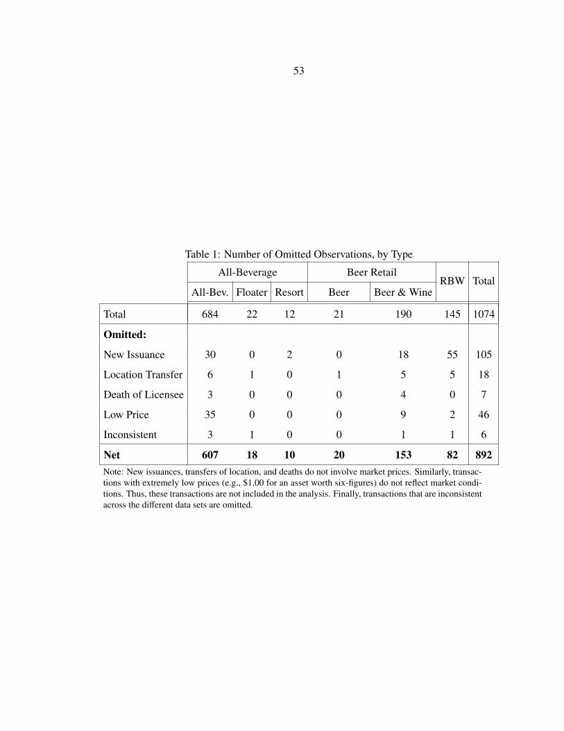
53
Table 1: Number of Omitted Observations, by Type
All-Beverage Beer RetailRBW Total
All-Bev. Floater Resort Beer Beer & Wine
Total 684 22 12 21 190 145 1074
Omitted:
New Issuance 30 0 2 0 18 55 105
Location Transfer 6 1 0 1 5 5 18
Death of Licensee 3 0 0 0 4 0 7
Low Price 35 0 0 0 9 2 46
Inconsistent 3 1 0 0 1 1 6
Net 607 18 10 20 153 82 892Note: New issuances, transfers of location, and deaths do not involve market prices. Similarly, transac-tions with extremely low prices (e.g., $1.00 for an asset worth six-figures) do not reflect market condi-tions. Thus, these transactions are not included in the analysis. Finally, transactions that are inconsistentacross the different data sets are omitted.

54
Table 2: Number of Usable Observations, by County and YearCounty 2005 2006 2007 2008 2009 2010 2011 2012 TotalBeaverhead 2 0 1 1 1 2 4 2 13Big Horn 1 1 0 2 0 1 1 0 6Blaine 1 1 1 0 0 1 0 0 4Broadwater 1 3 1 0 0 1 0 1 7Carbon 3 3 3 2 3 1 4 1 20Carter 0 0 0 0 0 0 0 0 0Cascade 12 12 3 6 2 3 1 2 41Chouteau 1 4 0 1 0 0 0 0 6Custer 3 2 0 2 3 0 2 0 12Daniels 1 1 0 2 0 0 0 1 5Dawson 1 2 1 2 0 0 2 0 8Deer Lodge 1 4 2 2 2 0 1 0 12Fallon 1 1 1 0 0 1 0 0 4Fergus 2 5 0 1 2 2 4 1 17Flathead 17 24 8 7 4 9 7 3 79Gallatin 13 13 13 10 12 11 10 10 92Garfield 0 0 0 1 0 0 0 0 1Glacier 3 2 0 1 0 2 0 0 8Golden Valley 0 0 0 0 0 0 0 0 0Granite 1 2 0 1 0 1 1 0 6Hill 2 2 1 2 0 3 1 1 12Jefferson 3 4 3 1 1 0 1 1 14Judith Basin 1 0 4 0 0 0 0 2 7Lake 6 4 3 1 2 0 1 0 17Lewis & Clark 8 4 3 1 3 3 4 2 28Liberty 0 1 0 0 0 0 0 0 1Lincoln 1 5 2 1 0 3 3 2 17Madison 4 7 1 1 4 2 2 5 26McCone 1 1 0 0 1 0 1 1 5Meagher 1 2 0 1 0 1 1 1 7Mineral 1 2 0 0 0 0 0 0 3Missoula 7 6 8 2 5 14 5 13 60Musselshell 1 0 1 0 1 0 0 0 3Park 2 4 8 2 3 1 6 1 27Petroleum 0 0 0 0 0 0 0 0 0Phillips 2 0 1 4 1 3 0 0 11Pondera 0 1 1 0 0 0 1 0 3Powder River 0 0 2 0 1 0 0 0 3Powell 2 1 1 2 0 1 1 1 9Prairie 0 0 0 0 0 0 0 0 0Ravalli 6 10 3 2 1 6 5 1 34Richland 1 2 1 0 0 1 3 3 11Roosevelt 0 2 0 2 2 0 1 2 9Rosebud 0 0 1 1 0 1 2 0 5Sanders 3 1 3 1 0 2 0 2 12Sheridan 1 0 0 0 1 1 0 2 5Silver Bow 10 16 10 7 9 4 4 1 61Stillwater 2 1 1 0 1 1 0 2 8Sweet Grass 0 1 0 0 1 0 2 0 4Teton 3 1 0 3 1 0 1 2 11Toole 3 1 1 0 1 1 0 1 8Treasure 1 0 0 0 1 0 0 0 2Valley 4 4 2 1 2 2 2 2 19Wheatland 0 1 0 0 0 1 0 0 2Wibaux 0 0 0 0 0 1 0 0 1Yellowstone 20 21 17 6 13 6 16 7 106Total 160 185 112 82 84 93 100 76 892Note: Carter, Golden Valley, Petroleum, and Prairie counties do not observe anytransactions for 2005-2012.

55
Table 3: Average All-Beverage License Price (Nominal), By City and Year
2005 2006 2007 2008 2009 2010 2011 2012
City Price n Price n Price n Price n Price n Price n Price n Price n
Billings 417,222 9 501,722 9 677,333 9 866,667 3 698,333 6 800,000 1 404,500 3 318,500 2
Missoula 512,500 2 623,333 3 679,167 6 0 750,000 1 694,167 6 798,333 3 630,000 5
Great Falls 392,000 5 336,667 6 360,000 3 437,500 2 400,000 1 375,000 1 425,000 1 312,500 2
Bozeman* 500,000 1 611,250 2 850,000 1 875,000 2 318,750 2 25,500 2 425,267 3 600,000 1
Butte* 30,500 5 35,714 7 60,625 8 66,400 5 67,750 8 50,000 2 40,000 2 45,000 1
Helena* 350,000 1 0 412,500 2 485,000 1 566,667 3 400,000 1 650,000 1 575,000 1
Kalispell 425,000 3 625,000 3 200,000 2 0 0 625,000 1 399,500 2 0
Havre 138,133 1 0 110,000 1 120,000 1 0 20,000 1 75,000 1 0
Anaconda* 15,000 1 22,500 2 31,250 2 10,000 1 42,000 2 0 0 0
Miles City 66,667 3 65,000 2 0 172,500 2 140,000 1 0 150,000 1 0
Belgrade* 500,000 1 600,000 2
Livingston 55,000 2 60,000 2 100,000 3 130,000 1 97,500 2 100,000 1 125,000 1 58,000 1
Laurel 30,000 1 295,000 2 475,000 2 0 365,000 1 0 0 0
Whitefish* 306,667 3 260,000 2 650,000 1 297,500 2 320,000 1 450,000 1 400,000 1 300,000 1
Lewistown 0 85,000 2 0 200,000 1 70,000 1 100,000 1 150,000 1 0
Montana 131,180 102 179,893 89 235,110 80 154,061 60 198,864 49 162,856 52 188,761 47 180,159 38*Belgrade and Bozeman merged quota areas in 2006. Similarly, Butte and Silver Bow County, Helena and East Helena, Anaconda and DeerLodge County, and Whitefish and Columbia Falls are each joint quota areas, with the numbers reported as such.

56
Table 4: Household Median Income (Nominal), by County
County 2005 2006 2007 2008 2009 2010 2011 2012
Yellowstone 41,171 43,407 47,947 49,337 47,139 48,059 47,346 49,405
Missoula 41,283 38,880 42,598 43,260 40,130 44,084 42,082 44,320
Flathead 39,917 44,413 45,122 44,013 45,594 42,278 44,006 45,742
Gallatin 45,312 46,928 50,511 53,042 47,065 49,354 50,042 51,394
Cascade 37,877 39,146 41,999 42,528 40,434 41,827 42,525 42,192
Lewis & Clark 45,299 44,382 46,647 49,959 52,317 50,889 52,510 54,096
Ravalli 36,914 39,872 42,450 43,613 40,444 39,409 39,421 38,445
Silver Bow 33,414 34,739 40,053 38,439 40,055 37,851 39,586 39,835
Lake 35,751 34,668 34,732 38,505 35,888 35,558 37,135 33,021
Lincoln 30,407 32,956 33,680 33,383 32,676 33,908 33,656 34,764
Hill 35,868 37,349 39,155 40,341 40,778 39,678 42,014 41,194
Park 35,761 36,630 40,173 39,847 39,525 37,835 42,332, 40,399
Glacier 30,285 29,954 36,054 36,149 29,941 32,460 33,766 34,508
Big Horn 30,680 31,705 33,004 37,798 32,223 34,507 34,778 36,322
Fergus 34,251 35,922 37,259 39,561 37,402 37,669 38,912 40,114
Montana 38,503 40,299 43,000 43,948 42,222 42,303 44,011 45,030Source: U.S. Census Bureau Small Area Income and Poverty Estimates.

57
Table 5: Unemployment, by County
County 2005 2006 2007 2008 2009 2010 2011 2012
Yellowstone 2.9 2.7 2.6 3.4 4.4 5.2 4.9 4.4
Missoula 3.3 3.0 3.3 4.4 5.6 6.7 6.3 5.9
Flathead 4.1 3.6 3.8 6.0 10.4 11.0 10.2 9.0
Gallatin 2.6 2.3 2.5 3.7 6.1 6.5 5.9 5.3
Cascade 3.6 3.1 3.3 4.1 4.8 5.6 5.8 5.4
Lewis & Clark 3.3 3.0 2.9 3.7 4.4 5.1 5.1 4.9
Ravalli 4.4 3.9 4.3 5.8 8.1 9.0 8.8 8.0
Silver Bow 3.8 3.5 3.5 4.3 5.5 5.8 6.0 5.8
Lake 4.9 4.5 5.3 6.7 8.2 9.4 9.8 8.9
Lincoln 3.9 2.9 2.8 3.7 3.8 5.5 4.9 5.3
Hill 3.8 3.6 3.9 4.5 4.8 5.1 5.6 5.5
Park 3.5 3.1 3.4 4.7 7.0 7.5 7.2 6.4
Glacier 6.6 6.3 7.7 8.2 8.2 9.4 11.2 10.2
Big Horn 7.7 6.4 6.4 7.4 8.4 10.8 12.0 12.8
Fergus 4.4 3.9 3.8 4.2 4.8 5.9 5.7 5.3
Montana 3.9 3.3 3.4 4.6 6.3 6.9 6.6 6.0Source: U.S. Bureau of Labor Statistics Local Area Unemployment Statistics.Note: units are percentage points.

58
Table 6: Annual Population Growth Rate, by City
County 2005 2006 2007 2008 2009 2010 2011 2012
Billings 1.6 1.3 1.3 1.9 1.5 1.2 1.0 1.4
Missoula 1.5 2.2 1.8 1.7 1.0 0.9 0.8 1.3
Great Falls -0.2 0.0 0.2 0.6 0.3 1.3 0.4 -0.1
Bozeman 4.2 4.7 3.2 2.8 0.5 0.6 2.1 1.6
Butte 0.0 0.1 0.1 1.0 0.6 0.7 0.4 0.1
Helena 0.2 1.1 1.3 1.3 1.0 1.2 1.4 1.5
Kalispell 3.4 3.8 3.7 3.1 1.5 0.7 1.5 1.1
Havre -0.4 0.7 0.3 -0.9 0.6 2.4 1.6 0.1
Anaconda 0.0 -1.0 0.9 0.9 -1.0 0.5 -0.7 -0.2
Miles City -0.9 -0.4 0.6 0.1 1.0 0.3 1.0 1.0
Belgrade 3.8 4.2 2.9 2.4 -0.1 0.2 1.4 .8
Livingston 0.7 0.3 0.8 0.4 -1.1 -1.0 -0.4 0.8
Laurel 0.8 0.7 0.7 1.3 0.9 0.8 1.3 1.6
Whitefish 1.3 1.7 1.7 1.1 -0.4 -0.8 0.5 1.2
Lewistown -1.7 -0.3 -1.2 -1.0 0.2 -0.3 -0.6 -0.4
Montana 1.1 1.3 1.3 1.2 0.8 0.7 0.7 0.7Source: U.S. Census Bureau City and Town Intercensal Estimates.Note: units are percentage points.

59
Table 7: University Enrollment, by City/County
City/County 2005 2006 2007 2008 2009 2010 2011 2012
Missoula 13,569 13,925 13,628 14,207 14,921 15,642 16,669 14,946
Bozeman 12,143 12,052 11,932 11,976 12,348 13,081 13,671 14,379
Billings 4,828 4,596 4,651 4,259 4,513 4,788 6,316 6,168
Great Falls 2,653 2,676 2,790 2,944 3,300 2,707 2,949 2,839
Helena 2,376 2,233 2,446 2,589 2,842 2,973 3,145 3,090
Butte 2,234 2,357 2,347 2,402 2,694 2,864 2,803 2,816
Kalispell 2,094 1,878 1,911 1,899 2,501 2,539 2,495 2,395
Havre 1,347 1,359 1,215 1,217 1,275 1,304 1,273 1,282
Dillon 1,159 1,176 1,148 1,190 1,255 1,365 1,379 1,483
Lake Co. 1,142 1,092 1,040 993 1,204 1,158 1,112 906
Miles City 491 464 506 511 502 486 491 441
Browning 485 467 471 492 533 473 464 407
Glendive 549 466 446 414 441 560 443 312
Poplar 408 441 422 436 437 452 513 438
Rosebud Co. 554 359 437 443 472 433 374 361
Chouteau Co. 344 397 305 236 303 332 410 501
Big Horn Co. 259 312 272 337 415 410 366 325
Harlem 175 161 244 168 236 214 169 221Source: National Center for Education Statistics Integrated Postsecondary Education DataSystem.

60
Table 8: Hotel Tax Revenue (Nominal), by County
County 2005 2006 2007 2008 2009 2010 2011 2012
Yellowstone 1,825,915 2,050,573 2,361,740 2,419,192 2,356,489 2,481,541 2,841,937 3,101,854
Missoula 1,736,689 1,978,422 2,175,701 2,250,799 2,085,784 2,156,742 2,285,656 2,426,703
Flathead 1,700,598 1,880,401 2,125,504 2,186,500 1,928,873 2,204,580 2,341,672 2,722,194
Gallatin 3,401,413 3,693,597 4,249,929 4,200,722 3,689,634 4,079,062 4,399,477 4,878,447
Cascade 858,289 954,573 1,081,631 1,186,769 1,151,200 1,240,594 1,375,864 1,476,244
Lewis & Clark 707,756 773,436 855,148 862,092 842,786 857,801 966,884 990,194
Ravalli 195,404 210,040 224,676 220,614 196,619 214,173 227,716 245,852
Silver Bow 609,213 666,349 756,162 754,608 731,236 758,855 771,095 816,917
Lake 122,877 130,132 133,473 125,186 110,531 120,065 126,319 144,569
Lincoln 97,661 112,193 118,459 120,081 108,767 104,466 103,418 116,623
Hill 147,557 157,316 178,098 196,039 192,458 221,242 230,762 242,315
Park 669,431 741,764 840,488 903,613 873,911 968,324 980,788 1,065,924
Glacier 543,197 515,891 573,240 617,197 619,189 684,955 611,055 622,505
Big Horn 115,264 125,523 138,913 135,192 134,101 139,548 143,274 145,881
Fergus 101,001 107,088 122,021 132,254 92,255 124,447 134,450 136,668Source: Montana Department of Revenue.
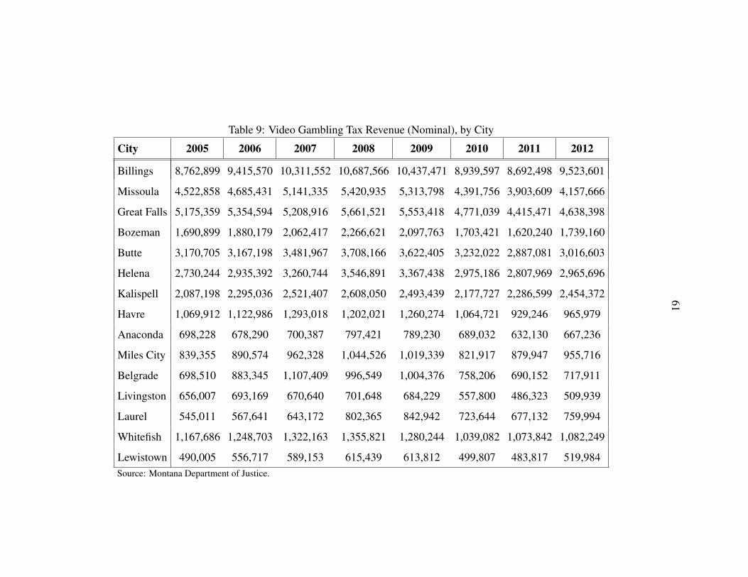
61
Table 9: Video Gambling Tax Revenue (Nominal), by City
City 2005 2006 2007 2008 2009 2010 2011 2012
Billings 8,762,899 9,415,570 10,311,552 10,687,566 10,437,471 8,939,597 8,692,498 9,523,601
Missoula 4,522,858 4,685,431 5,141,335 5,420,935 5,313,798 4,391,756 3,903,609 4,157,666
Great Falls 5,175,359 5,354,594 5,208,916 5,661,521 5,553,418 4,771,039 4,415,471 4,638,398
Bozeman 1,690,899 1,880,179 2,062,417 2,266,621 2,097,763 1,703,421 1,620,240 1,739,160
Butte 3,170,705 3,167,198 3,481,967 3,708,166 3,622,405 3,232,022 2,887,081 3,016,603
Helena 2,730,244 2,935,392 3,260,744 3,546,891 3,367,438 2,975,186 2,807,969 2,965,696
Kalispell 2,087,198 2,295,036 2,521,407 2,608,050 2,493,439 2,177,727 2,286,599 2,454,372
Havre 1,069,912 1,122,986 1,293,018 1,202,021 1,260,274 1,064,721 929,246 965,979
Anaconda 698,228 678,290 700,387 797,421 789,230 689,032 632,130 667,236
Miles City 839,355 890,574 962,328 1,044,526 1,019,339 821,917 879,947 955,716
Belgrade 698,510 883,345 1,107,409 996,549 1,004,376 758,206 690,152 717,911
Livingston 656,007 693,169 670,640 701,648 684,229 557,800 486,323 509,939
Laurel 545,011 567,641 643,172 802,365 842,942 723,644 677,132 759,994
Whitefish 1,167,686 1,248,703 1,322,163 1,355,821 1,280,244 1,039,082 1,073,842 1,082,249
Lewistown 490,005 556,717 589,153 615,439 613,812 499,807 483,817 519,984Source: Montana Department of Justice.

62
Table 10: All-Beverage License Quota and Licenses Issued
2005 2006 2007 2008 2009 2010 2011 2012
City Quota Issued Quota Issued Quota Issued Quota Issued Quota Issued Quota Issued Quota Issued Quota Issued
Billings 67 91 67 92 68 93 70 95 72 97 73 98 72 98 73 97
Missoula 44 70 44 70 45 70 47 71 48 72 48 72 47 73 47 73
Great Falls 40 79 41 80 41 81 42 83 42 84 42 84 42 84 42 84
Bozeman** 24 33 29 41 30 41 33 43 34 45 34 46 33 48 33 48
Butte* 25 86 25 85 25 85 24 85 24 87 24 87 25 87 25 86
Helena* 22 42 21 42 22 42 23 42 23 42 24 42 23 42 23 42
Kalispell 14 25 14 26 15 28 16 30 17 30 17 30 16 30 16 30
Havre 9 18 9 18 9 18 9 18 9 20 9 20 9 21 9 21
Anaconda* 9 35 9 34 9 33 8 33 8 32 8 30 9 30 9 30
Miles City 8 20 8 20 8 20 8 20 8 21 8 21 8 21 8 21
Belgrade** 7 8
Livingston 7 20 7 20 7 20 7 20 7 21 7 21 7 21 7 21
Laurel 7 10 7 10 7 10 7 10 7 10 7 10 7 10 7 10
Whitefish* 9 23 10 23 10 23 11 24 12 24 12 24 10 24 10 24
Lewistown 7 11 7 11 7 11 6 11 6 15 6 15 6 15 6 15*The numbers include other towns within ten miles; the five mile buffers overlap, resulting in joint determination of quota.**Bozeman and Belgrade merged quota areas in 2006.
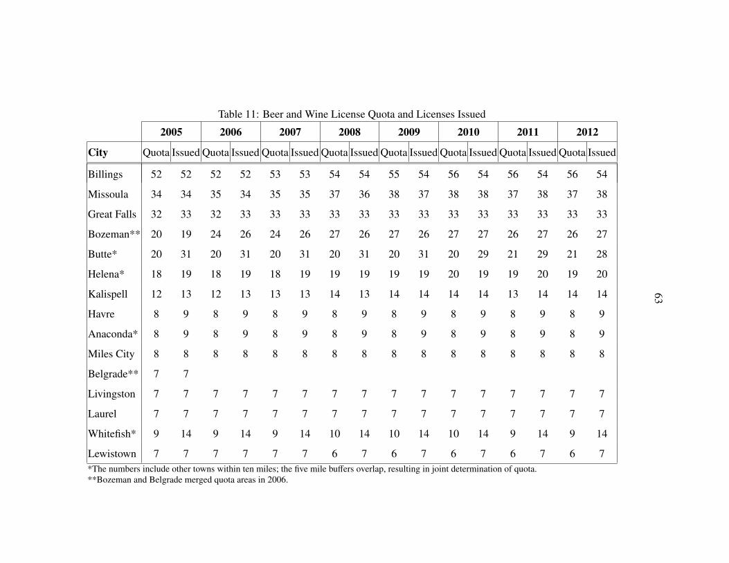
63
Table 11: Beer and Wine License Quota and Licenses Issued
2005 2006 2007 2008 2009 2010 2011 2012
City Quota Issued Quota Issued Quota Issued Quota Issued Quota Issued Quota Issued Quota Issued Quota Issued
Billings 52 52 52 52 53 53 54 54 55 54 56 54 56 54 56 54
Missoula 34 34 35 34 35 35 37 36 38 37 38 38 37 38 37 38
Great Falls 32 33 32 33 33 33 33 33 33 33 33 33 33 33 33 33
Bozeman** 20 19 24 26 24 26 27 26 27 26 27 27 26 27 26 27
Butte* 20 31 20 31 20 31 20 31 20 31 20 29 21 29 21 28
Helena* 18 19 18 19 18 19 19 19 19 19 20 19 19 20 19 20
Kalispell 12 13 12 13 13 13 14 13 14 14 14 14 13 14 14 14
Havre 8 9 8 9 8 9 8 9 8 9 8 9 8 9 8 9
Anaconda* 8 9 8 9 8 9 8 9 8 9 8 9 8 9 8 9
Miles City 8 8 8 8 8 8 8 8 8 8 8 8 8 8 8 8
Belgrade** 7 7
Livingston 7 7 7 7 7 7 7 7 7 7 7 7 7 7 7 7
Laurel 7 7 7 7 7 7 7 7 7 7 7 7 7 7 7 7
Whitefish* 9 14 9 14 9 14 10 14 10 14 10 14 9 14 9 14
Lewistown 7 7 7 7 7 7 6 7 6 7 6 7 6 7 6 7*The numbers include other towns within ten miles; the five mile buffers overlap, resulting in joint determination of quota.**Bozeman and Belgrade merged quota areas in 2006.

64
Table 12: Restaurant Beer and Wine License Quota and Licenses Issued
2005 2006 2007 2008 2009 2010 2011 2012
City Quota Issued Quota Issued Quota Issued Quota Issued Quota Issued Quota Issued Quota Issued Quota Issued
Billings 21 19 21 19 42 25 43 30 44 33 45 35 45 41 45 43
Missoula 14 17 14 17 28 21 30 25 30 28 30 29 30 29 30 30
Great Falls 16 10 16 10 32 11 33 12 33 13 33 14 33 14 33 14
Bozeman** 10 11 12 13 24 15 27 18 27 26 27 27 26 27 26 27
Butte* 10 1 10 1 20 2 20 2 20 1 20 3 21 3 21 3
Helena* 9 10 9 10 18 13 19 16 19 17 20 18 19 19 19 19
Kalispell 10 10 21 12 14 14 14 14 14 14 14 14 21 14 14 17
Havre 6 0 6 0 13 1 13 1 13 1 13 1 13 1 13 1
Anaconda* 6 0 6 0 13 0 13 0 13 0 13 0 13 0 13 0
Miles City 6 0 6 0 13 0 13 0 13 0 13 0 13 1 13 1
Belgrade** 6 2
Livingston 6 0 6 0 11 2 11 3 11 4 11 4 11 4 11 3
Laurel 6 0 6 0 11 0 11 0 11 0 11 0 11 0 11 0
Whitefish* 9 10 9 10 18 13 20 16 20 18 20 20 18 20 18 20
Lewistown 6 3 6 3 11 3 10 3 10 2 10 3 10 5 10 5*The numbers include other towns within ten miles; the five mile buffers overlap, resulting in joint determination of quota.**Bozeman and Belgrade merged quota areas in 2006.
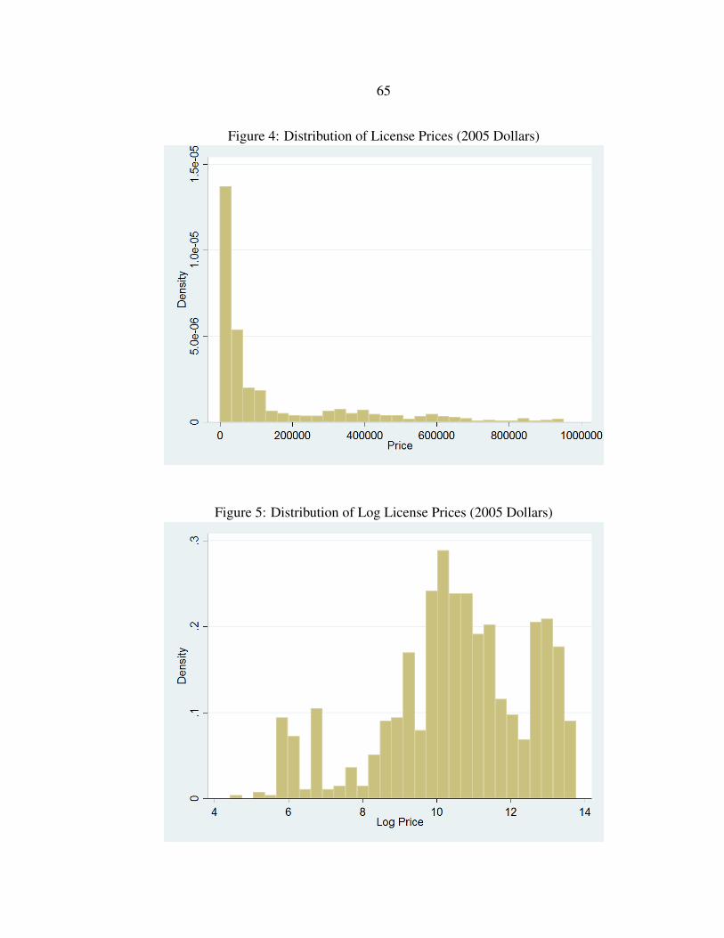
65
Figure 4: Distribution of License Prices (2005 Dollars)
Figure 5: Distribution of Log License Prices (2005 Dollars)

66
Table 13: Means and Standard Deviations, by YearYear Log Price Gamb. Rev. Hotel Rev. Population % 20-44 % Female Enrollment Med. Inc. Unemp.2005 10.44 13961 13683 27576 30.66 49.79 1954 37975 3.67
(2.09) (18626) (14321) (31101) (5.18) (1.57) (3480) (4842) (0.94)2006 10.32 13387 13863 27664 29.76 49.81 1819 37941 3.40
(2.12) (17920) (14835) (30226) (5.04) (1.26) (3463) (4944) (0.91)2007 10.87 16051 18231 30028 30.61 49.62 2256 40104 3.41
(2.04) (20946) (18094) (33025) (6.05) (1.47) (3874) (5559) (1.01)2008 10.58 11011 14990 21488 29.61 49.46 1568 38340 4.71
(1.84) (16561) (17763) (27055) (6.12) (1.98) (3206) (5699) (1.41)2009 10.66 17658 17109 32751 30.20 49.62 3023 38511 5.56
(1.87) (21116) (16799) (34976) (6.38) (1.22) (4520) (4758) (1.50)2010 10.85 11774 17435 28956 30.42 49.49 4164 37699 7.27
(1.76) (13714) (17428) (29771) (6.57) (1.53) (6141) (5036) (2.61)2011 10.30 12095 17281 29665 29.44 49.67 2593 38303 6.47
(1.90) (16911) (18225) (35670) (5.69) (1.46) (4323) (4622) (2.42)2012 10.53 12595 19588 31087 30.79 49.17 4534 38524 5.82
(1.95) (16226) (20864) (35174) (7.07) (1.70) (6204) (5347) (2.22)Total 10.54 13628 16032 28507 30.18 49.63 2551 38374 4.73
(1.99) (18065) (16940) (31973) (5.85) (1.51) (4411) (5103) (2.14)Note: Standard Deviations are reported in parentheses below the variable mean. Gambling and Hotel revenue are reported in thousands.

67
Table 14: Means and Standard Deviations, by CityYear Log Price Gamb. Rev. Hotel Rev. Population % 20-44 % Female Enrollment Med. Inc. Unemp.Billings 12.15 58967 30863 101286 32.51 51.16 5012 42534 3.58
(1.61) (4816) (3609) (3346) (0.37) (0.08) (700) (1347) (0.97)Missoula 12.43 27472 28038 66130 38.96 49.75 14763 38770 5.23
(1.29) (3404) (1458) (2117) (0.24) (0.07) (817) (1438) (1.48)Great Falls 12.38 33185 13888 57665 32.20 50.21 2755 37899 3.78
(1.28) (2691) (1759) (524) (0.46) (0.13) (151) (752) (0.83)Bozeman 11.85 15945 52493 42788 41.86 48.09 12715 44923 4.51
(1.32) (2964) (3632) (4081) (0.66) (0.12) (832) (1573) (1.73)Butte 10.37 20853 9457 33699 30.03 49.76 2460 34872 4.29
(0.80) (1451) (458) (334) (0.30) (0.24) (207) (1546) (0.96)Helena 12.32 22150 11230 29812 30.14 50.67 2738 45429 4.09
(1.16) (2017) (697) (914) (0.52) (0.04) (343) (1409) (0.93)Kalispell 11.97 14328 26948 18885 29.80 50.11 2150 40366 6.22
(1.90) (921) (2425) (1088) (0.71) (0.04) (264) (1737) (3.04)Havre 10.57 6726 2538 9357 30.73 49.64 1294 36050 4.54
(1.89) (876) (355) (186) (0.37) (0.18) (53) (508) (0.80)Anaconda 9.84 4482 438 9249 26.74 47.59 0 30730 5.47
(0.87) (322) (23) (61) (0.22) (0.33) (0) (1016) (1.07)Miles City 10.62 5806 3172 8335 28.02 50.44 493 35059 3.72
(1.68) (424) (584) (87) (0.53) (0.17) (15) (1309) (0.51)Total 10.54 13628 16032 28507 30.18 49.63 2551 38374 4.73
(1.99) (18065) (16940) (31973) (5.85) (1.51) (4411) (5103) (2.14)Note: Standard deviations are reported in parentheses below the variable mean. Gambling and Hotel revenue are reported in thousands. Hotelrevenue, percent ages 20-44, percent female, household median income, and unemployment are county-level figures.

68
RESULTS
Baseline Specifications
The initial specification employs a pooled-OLS model with a log-level functional
form, including all usable observations.48 The baseline results are reported in table 15.49
Column 1 does not include any variable relating to the supply of licenses. Column 2
reports estimates using percentage of all-beverage quota and indicator variables for
binding beer and wine and RBW quotas. Column 3 explicitly includes the number of
licenses issued. For the ease of interpretation, the regression measures gambling revenue
and hotel revenue in millions of dollars. Along the same lines, population, enrollment, and
household median income are measured in thousands.
In the first column, the specification provides evidence that gambling revenue,
hotel revenue (used as a proxy for tourism), college enrollment, and income are
statistically an economically significant positive determinants of license price. The
coefficient on gambling revenue, for example, indicates a 15 percent increase in license
price for million-dollar increase in gambling revenue. Similarly, the the estimated effect of
income is a 5.6 percent increase in license prices for an additional $1,000 in median
income, while enrollment pushes up prices by 23 percent for an additional 1,000 students.
The coefficient on enrollment, however, is not entirely plausible—more than half of
48The dummies for potential clerical errors are omitted throughout the section. The results across specifi-cations are robust to the inclusion of the variables, and are robust to the exclusion of the flagged observations.
49Historic market conditions might be expected to influence license prices, particularly if adaptive expec-tations are assumed. Including lagged independent variables, however, does not qualitatively change theanalysis. Several estimates are somewhat peculiar, however, with current and past period coefficients beingequal in magnitude but opposite in sign.

69
typical students are not legally permitted to consume alcohol. Thus, the effect is probably
overstated. Hotel revenue is less significant, both in statistical and economic terms. For an
additional million dollars of hotel revenue, license prices would only be expected to
increase by 1.6 percent. This result, moreover, is more sensitive to specification than the
other coefficients.
Several results are somewhat unexpected. First, unemployment is positive and
significant. While there are no ex ante expectations for the sign of unemployment, the
magnitude and significance of the coefficient are peculiar. The coefficient is not
particularly plausible—a 12 percent increase in license prices for a 1 percentage-point
increase in unemployment seems quite large. Concern over the estimate should be
tempered, however, for two reasons. First, the effect of unemployment is more sensitive to
functional form than the other variables.50 Second, it appears that the variation driving the
result may be from outliers. For 2009-2012, prices in Flathead County tend to be in the
six-figure range, even though unemployment spikes to double-digit levels. Similarly,
several of the counties with the lowest unemployment rates tend to have the lowest
prices.51 Running the regression without these observations decreases the coefficient
estimate to 0.09, while significance decreases to the 10 percent level. Although the
estimated effect remains high, the 95-percent confidence interval includes more plausible
magnitudes for short-run effects.52
50The variable is still significant in a level-level model, but significance largely disappears with a log-logfunctional form. Similarly, none of the fixed-effect specifications attribute a significant effect to unemploy-ment.
51These include Chouteau, Fallon, McCone, Richland, Stillwater, Sweet Grass, and Toole counties. Thesecounties account for 15 observations, while Flathead accounts for 79.
52In the long run, an increase in unemployment should produce a negative effect as incomes decrease.
70
Second, the coefficient on the percentage of the population that is female is
positive and significant at the 10 percent level. Again, there is no prediction regarding the
sign. The result is not as statistically strong as the others and is moderately sensitive to
specification. As is the case with unemployment, the identifying variation appears to be
concentrated in a small area. Billings has the highest female population in the state (by
number and percentage), along with the highest license values. Running the regression
without Billings results in percent female becoming insignificant (the other variables
remain significant).
Finally, the fact that population is estimated to have a negative effect is rather
perplexing. Holding other demand factors constant, the effect of increasing population
should be small. More people who gamble less (on average) should have a smaller impact
on price than an increase in population without controlling for other factors. Holding
percentage of quota constant, moreover, might be expected to cause population to have a
negative effect. In Column 2, the number of licenses implicitly increases with population,
holding gambling, tourism, and enrollment constant.53 Holding the number of licenses
constant, however, should at least attenuate this result.54 The quotas are set via population,
however, so the estimates may suffer from endogeneity bias with respect to license supply.
Of additional interest are the coefficients assigned to the license type and
transaction type indicator variables.55 As expected, the results indicate that all-beverage
53An increase in population, with a corresponding increase in licenses but less gambling/tourism/studentson average, would mean less gambling revenue and fewer tourist/students spread out over a larger number oflicensees.
54The results is not sensitive to functional form. Including a squared population term, or specifying popu-lation in logarithmic terms does not change the the qualitative result.
55All-beverage and transfer of ownership and location are the omitted variables.
71
licenses trade at a large premium over each of the the other license types. Although floater
licenses allow the same privileges as all-beverage licenses (except for gambling on floaters
issued after 2007), the results indicate that they are sold for 70 percent less on average.56
The prices on floaters, however, tend to reflect the market conditions from the license
seller’s area, not the buyer’s. The state issues floaters one at a time, allocating them via
lottery. Whoever wins the lottery goes to a lower-price market to purchase a license. The
buyer acts as a monopsonist, purchasing a license near the seller’s market price.
The disparity between all-beverage and the other two license types (beer and wine
retail and RBW licenses), on the other hand, reflects the differences in the privileges
associated with each license type. Beer retail licensees may offer the same services as
all-beverage licensees, with the notable exception of selling liquor. The discount for beer
and wine licenses is estimated at 52 percent, on average. RBW licensees may not sell for
off-premises consumption, nor may they offer gambling under any circumstances.
Additionally, the more stringent constraints (e.g., the revenue requirement for food sales)
on RBW licenses should push prices down even further. The results provide evidence to
this effect, estimating that RBW licenses sell for 90 percent less than all-beverage licenses.
Given that state law allows gambling exclusively in establishments licensed to sell
alcohol, gambling revenue appears to affect the price of licenses in the expected manner.
Licenses that preclude gambling should sell for lower values. The coefficient on gaming
restrictions measures the relative difference in price between licenses with and without
gambling attached.57 The estimate (-0.897) is negative and both economically and
56Employing the transformation described above: 100 · (exp{−1.196} − 1) = −69.7657The dummy variable only takes on a value of 1 for all-beverage, floater, and beer and wine retail licenses.
72
statistically significant, predicting a 63 percent discount for gaming restricted licenses. A
point of caution, however, is that the variation driving the estimate comes almost
exclusively from beer and wine retail licenses.58
More intriguing is the coefficient for transfers of ownership (TRF-O). Ex ante, the
prices associated with the transfers of ownership (but not location) are expected to be
lower. It may be easier to obtain a larger loan if hard assets (i.e., land and a physical
structure) are acquired with a license. As a result, there may be an incentive to
(marginally) adjust how much value is assigned to a license versus a building. Similarly, a
transaction may involve a lower price if an establishment and a licenses are purchased
simultaneously. The estimated effect is negative and significant, supporting the
predication that licenses attached to a location trade at lower values—the magnitude of the
discount is slightly less than 30 percent. Not all transfers of ownership involve the sale of
a building, however. Thus, the estimate should serve as a lower bound on the estimated
effect of purchasing a license with physical property.
The sign on the coefficients for the other two transaction types(corporate structure
change and the missing transaction type) are negative, as expected. The estimated
discount for CSCs, moreover, is significant at the 10 percent level. The significance is
somewhat surprising, given the high variation in price for CSCs (a CSC may range from a
partial buy-out to a full transaction).
Columns 2 and 3 add controls for percentage of quota and number of licenses
Restaurant licenses may not offer gambling under any circumstances. Thu, they are not flagged as “gamingrestricted’.
58Of the observations flagged as gaming restricted, 18 are beer and wine licenses, 9 are floaters, and 1 isan all-beverage license.

73
issued, respectively. The results for the variables in the first column are fairly robust to the
inclusion of either set of controls for the supply of licenses. The qualitative interpretations
of the effects are quite similar, with the exception of losing significance on the coefficient
for hotel revenue. The coefficients on the continuous variables, however, tend to decrease
by around one standard error. The results for the license and transaction type variables are
qualitatively identical.
The similarity in the qualitative results indicates that there is probably is not
enough evidence to reject the idea that simultaneity bias is limited with respect to the
variables other than population. Treating license supply as exogenous (with respect to
everything but population) is consistent with the institutional details of the Montana
licensing system. This is particularly true for the supply of all-beverage licenses, at least
within any given year. For the other license types, exogeneity is somewhat less likely to
hold, as beer and wine licenses are not always limited by a quota. Although simultaneity
bias is not necessarily expected ex ante, it is still possible that the specification could
suffer from bias if the supply of licenses is endogenous with respect to the other variables.
The variables for license supply are also significant, which increases concerns over
potential bias in the coefficient estimates. That said, only the RBW supply variables are
significant across both Column 2 and Column 3. Percentage of the all-beverage quota and
and percentage squared are significant in Column 2, but all-beverage licenses issued is not
significant in Column 3. Similarly, the supply variables for beer and wine is not significant
across both. Given that significance is sensitive to whether supply is specified in relative
or absolute terms, the results should not be overly concerning.

74
Subsamples
As robustness checks, similar regression specifications may be run on subsets of
the data to test for differential effects. The baseline specifications include data from all of
the quota areas that recorded usable transactions. There are reasons to believe, however,
that the identifying variation is coming from a subset of the data. To evaluate that idea,
regressions are run on a restricted sample and on all-beverage licenses only.
To restrict the sample, several criteria are used. First, the specifications drop
additional low-priced transactions. The logic for doing so is consistent with that outlined
above. While not as extreme as $1.00 sales, a price of $10,000 in a market that routinely
assigns six-figure values to licenses raises concerns about the nature of such transactions.
Relative to a more typical, higher-priced sale, the low price probably reflects unobserved
factors in the transaction. Thus, the specifications drop observations listing a license price
more than two standard deviations below the quota-area/transaction type mean (taken over
time).
Similarly, the specification only includes transactions from areas at or above their
all-beverage quotas.59 If the license quota is non-binding in an area, the expected price
should be quite close to zero. This is frequently borne out in the data, with prices in many
non-binding areas mirroring the annual licensing fee.60 If a quota area employs fewer
licenses than permitted by law, marginal changes in demand factors should have little to
59For the purposes of the regression, “at or above” included areas above 100 percent of quota.60The license fees tend to be $400-$650, depending on population and license type. For a full listing of
license fees, see M.C.A. 16-4-501.

75
no impact on license price.
A caveat to the non-binding quotas is the licenses attached to businesses near
incorporated areas. As communities expand, so too does the five-mile buffer around city
limits. If a license is absorbed into the quota area, it potentially gains a great deal of value.
As such, the value of an unincorporated license in Gallatin or Missoula County near
Bozeman or Missoula, respectively, may be influenced by the market conditions of the
nearby quota areas. A similar price effect may persist, even well beyond the five-mile
buffer. Tourist locations near a major city, for example, may be well outside the buffer, but
still push up license prices.61
Finally, the specifications include only transfers of ownership and transfers of
ownership and location (omitting corporate structure changes and observations missing
transaction type). Focusing on full sales may provide better estimates, as the effects of
market forces may be muted on the other transaction types. If the prices of many CSCs
reflect the values associated with different-sized partial financial interests, the estimated
effects may not be as clean. Unfortunately, observations missing the transaction type are
also omitted, as there is no way to identify if they are full sales or not.62
Table 16 reports the results from employing the restricted data set, following the
same pattern as the results reported above. Column 1 omits any control for license supply,
while Columns 2 and 3 include quota percentages and licenses issued, respectively.
Overall, the regressions include 595 data points, slightly more than two-thirds of the data.
61The highest license price observed in a non-binding quota area was from a 2006 sale in Missoula Countyat the Lolo Hot Springs near Missoula. The license sold for $400,000.
62There are 66 CSCs in the data, and 70 missing transaction types.

76
The results are relatively consistent qualitatively with the specifications including all
usable observations, with a slightly improved fit.
The results in Column 1 identify the same significant effects as the baseline
specifications, although the magnitudes are somewhat attenuated. Particularly, the
estimated effects of gambling revenue, population, and enrollment are almost twice as
large in table 15 than in table 16. Although marginal changes in each variable might be
expected to have a larger effect on the restricted sample, many of the observations from
smaller areas are dropped. Thus, there is a less cross-sectional variation driving the results.
In contrast, the magnitude of the estimates on the indicator for license types
remain very consistent when the data set is restricted. The coefficients for floaters and and
beer and wine licenses increase slightly, while the estimated discount for beer and wine
licenses decreases slightly. The coefficient for restricted gaming licenses does not change
systematically compared to the original estimates. In each case, the changes are all within
a single standard error of the original estimates.
Table 16 only includes transfers of ownership and transfers of ownership and
location, dropping CSCs and observations missing the transaction type. Thus, the only
transaction variable included in the regression is that for transfers of ownership relative to
sales including a change in location. The estimated discount decreases to roughly 23
percent, although the coefficient is statistically identical to the baseline estimate.
Columns 2 and 3 add controls for quota percentages and licenses issued,
respectively. As before, the estimated effects are relatively robust to including controls for
license supply. The differences between the columns are smaller in table 16 than in the
77
baseline regressions. Unlike the previous results, however, hotel revenue is only
significant when percentage of quota is controlled for (although the point estimate is
relatively constant). In addition, the results for population and unemployment are less
robust. Again, this is probably due to the reduction in cross-sectional variation from
omitting observations. The rest of the coefficients, however, are within roughly one
standard error of each other across all three columns within table 16.
Overall, it appears that much of the variation driving the results comes from the
non-low price, full transfer transactions in binding quota areas. The qualitative results are
quite similar to the specifications including more observations, but with slightly decreased
magnitudes in several cases. These results are possibly better estimates of marginal
effects, as the restrictions on the data limit the sample to relatively similar areas, reducing
variation due to large differences across areas. While there is still a great deal of
identifying variation in the remaining observations, it is clear that some important
variation is still lost.
The second subsample of the data consists of all-beverage licenses exclusively. In
the baseline results presented in table 15, the coefficients of each explanatory variable is
restricted to having the same estimated value across all-beverage, beer and wine, and
RBW licenses. Optimally, the data would be expansive enough to run a fully interacted
model and test to see if the estimated effects are constant across each license type.
Similarly, separate regressions for each license type could be run to the same effect.
All-beverage licenses trade far more frequently than the other license types,
making up almost 70 percent of the observations. Unfortunately, the remaining

78
observations for the other license types are relatively sparse.63 Consequently, a fully
interacted model (or separate regressions exclusively on beer retail or RBW licenses) is
not a viable option. The large number of all-beverage transactions, however, make an
all-beverage exclusive specification feasible. Table 17 reports the results from dropping
non-all-beverage transactions.
The columns follow the same pattern as above, beginning with no supply variables
and reporting the alternative specifications in the the next two columns. The estimated
effects look virtually identical to the baseline results in terms of both significance and
magnitude. The only exceptions are the loss of significance of hotel revenue in Column 1
and an increase in significance for percent female in Column 2. Similarly, the results are
robust to the inclusion of the different variables for license supply, even more so than the
baseline results.
The robustness of the results to excluding non-all-beverage licenses provides
evidence that the effects are consistent across the different license types. This result is
unsurprising, as the vast majority of the data are comprised of all-beverage
transactions—the chance of finding differential effects is relatively small. A point of
interest is that the controls for beer and wine and RBW license supply are exogenous to
the all-beverage license market. The similarity in results between tables 15 and 17
supports that endogeneity bias is limited in the baseline specification.
Results are not produced combining the restrictions for the two different
63There are 173 Beer/Wine transactions and 82 RBW transactions. Running a regression on observationsother than all-beverage licenses produces similar results for gambling, population, enrollment, and transfersof ownership, losing significance for each of the other variables. In addition, hotel revenue is significant onright-tail test.
79
subsamples. If the data are restricted to full sales of all-beverage licenses in binding quota
areas, the sample size dwindles to just over 300. In addition to the small sample size
(which would only employ a little over a third of the usable data), both restrictions leave
relatively little cross-sectional variation. As such, there is very little to be gained by
narrowing the focus of the analysis any further.
Alternative Functional Forms
As an additional check for robustness, the model is specified across two alternative
functional forms: level-level and log-log. In addition to changing the interpretations of the
coefficients, specifying a model using different functional forms fundamentally changes
what the estimated relationships look like. If the results are robust across the different
functional forms, it provides additional evidence supporting the qualitative predictions of
the baseline model.
Table 18 reports the results produced using a level-level specification. Both the
dependent variable (license prices) and the independent variables are specified in level.
The estimated coefficients, then, represent the slope of the linear relationships between the
variables. The scale of several variables also differs in the level-level regressions, for ease
of interpretation. Rather than millions, gambling and hotel revenues are measured in
thousands. Population, enrollment, and household median income are all scaled back to
the original reported values.
Column 1 reports results that are qualitatively similar to the baseline output in table
15. Again, gambling revenue, hotel revenue, enrollment, and income are all identified as
80
significant positive determinants of license price. The quantitative interpretations,
however, are different. The estimated effects of an additional $1,000 in gambling and hotel
revenue are an increase in license values of $10.86 and $2.42, respectively. Enrollment is
also a major factor, with an estimated effect of around $20.00 for an additional student.
Similarly, for an additional dollar of income, the estimated effect is an increase license
prices by $7.72. While the interpretation of coefficients differ, the relative magnitudes of
the coefficients are also consistent across with the log-level models. Converting the
log-level estimates to dollar values at the mean license price, hotel revenue and income are
not statistically different between the two functional forms. The magnitude of gambling
revenue, however, is significantly smaller in the level-level model.64
Again, population, percent female, and unemployment are significant, with
slightly odd signs and magnitudes. The results are qualitatively similar to the baseline,
with percent female and unemployment being more sensitive to specification than the
other variables. In addition, the indicator variables for license and transaction type are
negative and consistent, also in line with the results in table 15. The magnitudes are also
easier to interpret.
All-beverage floaters trade at roughly $200,000 less than typical all-beverage
licenses. As mentioned above, floater prices reflect market conditions in the license
seller’s area, and tend to float to growing, high-priced markets. The estimated discount for
beer and wine licenses is around $55,000, while for RBW licenses the the average
difference in value compared to an all-beverage license is almost $300,000. Finally, the
64In the log-level model, the 15 percent increase in license prices for a $1 million dollar increase in gam-bling revenue translates into a $30 level change at the mean.

81
premium for gambling is just short of the anecdotal prediction of $250,000.65 These
estimates are quite large compared to the average price of an all-beverage license (around
$160,000 in the data set). Transactions involving floaters and RBW licenses, however,
tend to be observed in the higher-priced markets, which have an average all-beverage
price of around $450,000.66
The transaction type variables differ slightly in terms of significance. Compared to
the baseline results, table 18 reports that corporate structure changes are negative and
more statistically significant. While the signs match between the results, the significance
level is noticeably increased in the level-level specification. Conversely, transfers of
ownership decrease in significance. In Column 1, the coefficient on the indicator variable
is only significant at the 10 percent level on a left-tail test.67 The estimated discount is
slightly greater than $20,000.
Columns 2 and 3, which control for the supply of licenses, report very similar
results. The largest discrepancies between the specifications in table 18 are the loss of
significance in hotel revenue and simultaneous increase in significance of percent female
in Column 3. Similarly, while the variables for percentage of quota are insignificant in
Column 2, licenses issued for beer and wine and RBW licenses are highly significant in
Column 3. In light of the regression output in table 15, however, these results are quite
sensitive to specification, lending additional support that the supply of licenses is not
65According to Neil Peterson of the Gaming Industry Association of Montana, licenses with gamblingrights are worth around a quarter-million dollars more than a license without.
66The markets considered here are Billings, Missoula, Great Falls, Bozeman, Helena, Kalispell, and White-fish.
67It is appropriate to consider a left-tail test, as there is an ex ante prediction that the coefficient should beless than zero.

82
endogeneous with respect to the other variables (excepting population).
The second alternative functional form is log-log: the dependent variable is the
natural log of price, and several of the right-hand side variables are also specified in log
terms.68 In this case, the coefficients represent estimated elasticities, rather than linear
slopes. To interpret the coefficients on indicator variables, the same transformation used in
the log-level specification is required.
Table 19 presents the output from the log-log regressions. As is the case with the
level-level specifications, the log-log results in Column 1 are qualitatively similar to the
baseline output. The largest differences are the relative increase in magnitude of the effect
of hotel revenue, and the loss of significance on the coefficients for percent female and
unemployment. In contrast to the results in table 15, which had the effects of gambling
and hotel revenue differing by an order of magnitude, table 19 has them much closer.
Holding all else constant, a 1 percent increase in gambling or hotel revenue produces an
increase of 0.25 or 0.14 percent, respectively.
The estimated discounts for the different license and transaction types should all
have the same interpretations as the baseline. The overall results for the dummy variables,
while qualitatively similar, differ slightly in both magnitude and significance. The
estimated coefficients in table 19, Column 1, decrease in magnitude for floater and beer
and wine licenses by less than a standard error. The estimated discount for RBW licenses
also is closer to zero, but the difference is slightly greater. The largest difference between
the log-level and log-log models is the result for restricted gaming. Although the point
68Variables specified in percentage terms (e.g., unemployment) are left in levels. Similarly, licenses issuedare not specified in log terms.

83
estimate is within a standard error of the baseline result, significance decrease to the 10
percent level on a left-tail test. Conversely, the significance and magnitudes increase for
both CSCs and transfers of ownership.
Of the three functional forms, the log-log specifications are the least robust to the
inclusion of supply variables. Particularly, the estimated effects of gambling revenue,
population, enrollment, and income all vary significantly across Columns 1-3 in table 19.
For example, the estimated effect of a 1 percent increase in gambling revenue ranges 0.11
to 0.25, almost two standard errors difference. Population and enrollment show similar
sensitivity. More concerning is the lack of significance of income in Column 3. While the
first two columns report more than a 2 percent increase in license prices for a 1 percent
increase in income, including licenses issued causes the coefficient to lose all significance.
Given the sensitivity of the other variables to the inclusion of supply variables, it is
unsurprising that much of the explanatory power in the the log-log model is assigned to
the controls for license supply. Every supply variable is significant in table 19, with the
exception of RBW licenses issued (the only significant licenses issued variable in the
baseline specifications). Although the point estimates vary across the specifications in
table 19, the qualitative results are still very similar to those from the baseline regressions.
Fixed Effects
A third set of robustness checks consists of adding fixed effects to the regressions,
across each functional form. While the baseline regressions provide a descriptive analysis,
including fixed effects may help isolate causality in the right-hand side variables.
84
Including quota-area fixed effects conditions out systematic, time-invariant cross-sectional
variation (e.g., different drinking cultures or proximity to a tourist location). Similarly,
adding year fixed effects accounts for any variation caused by state-wide systematic
changes that are invariant across quota areas (e.g., the smoking ban that went into effect in
2009). Thus, the identifying variation is that which is exogenous to both the time invariant
differences between quota areas and the quota-area invariant differences across time.
Optimally, the remaining variation in the right-hand side variables will explain marginal
changes in the dependent variable, giving a better idea of the causal relationships between
variables.
As described above, including both sets of fixed effects conditions out a great deal
of variation. Particularly, in the context of alcohol retail license prices, their inclusion
drastically reduces the cross-sectional variation. Table 14 shows that the within-quota-area
standard deviations are quite small relative to the data set as a whole. Including quota-area
fixed effects leaves only that variation within the quota areas, which in turn is reduced by
year fixed effects. As a result, there is very little identifying variation left to drive
results—many coefficients are expected to be highly attenuated.
Table 20 reports the results from the log-level specifications with fixed effects,
including all usable observations. As expected, the regressions do not identify significant
effects for many of the covariates. Of the continuous variables, the coefficient on
population is the only one that remains statistically significant. Interestingly, the point
estimates in Columns 1 and 2 are not statistically different from the baseline results. Hotel
revenue nears significance on a right-tail test, with increased economic significance,
85
though the effect still remains questionable. For a million-dollar increase in hotel revenue,
license prices would only increase by 4 percent.69
While many of the continuous demand factors have no measurable effect, the
license type indicator variables are extremely robust to the inclusion of fixed effects.
Again, the estimated average discount of an all-beverage floater license relative to a typical
all-beverage license is just over 70 percent. Similarly, the estimated discount for beer and
wine retail licenses is 55 percent, while RBW licenses trade at a 92 percent discount.
Finally, the estimated effect of restricting gaming rights is a decrease in license price of 66
percent. Each result is qualitatively the same as in the baseline results reported in table 15.
Similarly, the estimated discount for transfers of ownership is consistently negative
and significant. The fixed effect estimates are noticeably smaller than the results in table
15, although the coefficients differ at most by only slightly more than a standard error. The
estimates in table 20 are still economically significant, putting the average discount for
transfers of ownership (compared to transfers of ownership and location) at just over 18
percent.
The estimated effects are almost identical across the three columns, with the
exception of the coefficient on population in Column 3. Although adding licenses issued
has little to no effect on most of the variables, it causes the estimated coefficient on
population to decrease dramatically. In Column 3, the estimated impact of increasing
population by 1,000 is a 20 percent decrease in license price.70 The coefficient on the
69Restricting the observations to higher-priced, full-sale transactions in binding quota areas, hotel revenuebecomes significant on a right-tail test, but the estimated effect declines.
70Again, licenses issued should be endogenous with respect to population, but not with the other variables.

86
number of beer and wine retail licenses issued also indicates a positive effect on license
prices. The estimated effect of an additional beer and wine license is an 11 percent
increase in license prices. Although the result is identical to that found in table 19, it is not
robust across the different specifications (indeed, table 18 reported a negative, highly
significant effect).
Table 21 reports results for the level-level specification with fixed effects. Several
differences between the results in table 21 and those from the baseline regressions are
immediately apparent. First, hotel revenue is consistently positive and significant, both
statistically and economically. For a $1,000 increase in hotel revenue, the estimated effect
is an increase of over $9.00 in license prices. On the other hand, the other continuous
variables lose significance, with the exception of gambling revenue and income. In
addition, population, enrollment, and unemployment change signs. Losing significance in
several variables is expected, as a great deal of identifying variation is lost with the
inclusion of fixed effects. Nonetheless, it is odd that the effects, for enrollment in
particular, change so drastically.
As is the case in for the log-level fixed effect results, several estimated effects are
very robust. Gambling revenue and household median income retain a high degree of
significance in table 21, with very consistent point estimates. Even more so than gambling
and income, the indicator variables for license type and transfer of ownership are robust to
adding fixed effects. The estimated discount for floaters remains just under $200,000; for
beer and wine licenses it stands at $55,000; for RBW licenses, the coefficient decreases
slightly, to -$300,000. Similarly, restricting gambling is estimated to push license prices

87
down by around $230,000, while transfers of ownership have a $20,000 average discount.
These results are qualitatively the same as the baseline results, and statistically identical to
those for the level-level results in table 18.
Finally, table 22 reports the results from the log-log fixed effect specifications. The
results are consistent across all three columns, in contrast to the results in table 19. As in
the log-level fixed effect specifications, gambling and hotel revenue have no measurable
impact on license prices.71 Similarly, population has a negative estimated effect that is
both statistically and economically significant. For a 1 percent increase in population,
each specification estimates a decrease in license prices by 2.3 - 3.9 percent. As in the
log-level models, the result is consistent with the baseline specifications.
The biggest difference between the log-log and the other fixed effect specifications’
results is the effect of enrollment. Neither of the other two models attributed a measurable
effect to the number of students in a quota area. In contrast, table 22 reports a positive
coefficient with a high degree of statistical significance. For a 1 percent increase in
university enrollment, license prices are estimated to increase by just over 0.2 percent.
This result, however, is consistent with the estimated effect in the baseline regressions.
The indicator variables for license type and transaction type have the same
interpretation as the log-level model. The qualitative and quantitative results remain the
same, as expected (log price is still the dependent variable). Each license type coefficient
is negative and significant at the 1 percent level, with the point estimates remaining
virtually identical to the log-level fixed effect results. Similarly, the results for transaction
71Additionally, hotel revenue does not approach significance.

88
type remain unchanged, with transfers of ownership having the only significant effect. As
is the case for the log-level fixed effect results, the estimated discounts for the different
license and transaction types in table 22 are not statistically different from the baseline
results.
With fixed effects included in the specifications, the results differ (particularly in
terms of significance) from the pooled OLS models. Similarly, the fixed effects results
differ substantially across the different functional forms. The probable cause of the
differences is that many of the explanatory variables do not differ much from the
quota-area fixed effects. In other words, there is more cross-sectional variation than
within-area variation. Thus, the inclusion of locational fixed effects leaves very little
residual variation to drive the results; the inclusion of time fixed effects eliminates even
more. Consequently, the various functional forms only pick up the effect of one or two
variables, given the limited identifying variation. Interestingly, the significant results in
each of the fixed effects regressions are consistent with the baseline, but none of the fixed
effect specifications pick up all of the effects simultaneously.
Thus, while the inclusion of fixed effects reduces the potential omitted variable
bias from unobserved heterogeneity, it also excludes enough variation to preclude
identifying any consistent effects. The relatively short length of the data set (8 years)
exacerbates the issue. Assuming that license prices factor in all future expected earnings,
year-to-year fluctuations in demand factors should not have large effects on license values.
This year-to-year variation is most of what is left to drive the results if quota-area fixed
effects are included. Given a longer time frame, the changes within quota area would

89
provide more information. With the relatively small number of years, however, it is
difficult to separate noise from long-term changes in demand factors.
Another confounding factor is that the markets are thinly traded (e.g., Bozeman
records roughly 2 full sales of all-beverage licenses each year). If licenses traded more
frequently, de-meaning the data with fixed effects might be the preferred methodology.
Marginal changes in the right-hand side variables would be more likely to cause marginal
changes in license prices. Given the relative sparseness of transactions in each year,
however, it is unlikely that license prices are very responsive to small changes in
gambling, tourism, enrollment, etc. Thus, looking at the large-scale differences across
areas may offer more information than examining smaller changes within quota areas.
Additional Robustness Checks
Although the log-level specification statistically outperforms the other functional
forms, there may still be value in additional checks as to which specification provides the
best fit for the data. A simple visual inspection of the fitted (predicted) values compared to
several independent variables provides an intuitive, straightforward test for fit.72
To produce the fitted values, the regressions are run omitting the independent
variable of interest. Fitted values are then extracted from the regression and plotted
against the omitted variable. Thus, the fitted values are different in each of the plots. If the
relationship looks systematic, the omitted variable probably contains important
information in predicting license prices. The plots provided are for three of the
72The fitted values refers to the predicted license prices: Y = βX. The vector X omits the independentvariable in question.
90
explanatory variables: gambling revenue, household median income, hotel revenue. The
first two are robust across the different specifications, while hotel revenue is more
sensitive to specification.
Figure 6 plots the relationship between fitted prices and gambling revenue for the
baseline log-level model (i.e., all usable data with no fixed effects). Figure 7 does the
same for a level-level specification, while figure 8 looks at a log-log functional form.
Visually, the relationship appears stronger for the log-level and level-level specifications
than for the log-log. The largest difference between figures 6 and 7 is the spread of the
data points around the linear fitted line. It slightly higher for the moderate values of
gambling revenue in figure 6, but lower towards the right tail. Otherwise, the two are hard
to distinguish between. The correlation between gambling revenue and the fitted values is
highest, however, in the level-level model (though only marginally).73
For household median income, figures 9-11 display the plots for fitted values
against household median income. Compared to the gambling revenue, there does not
appear to be a strong relationship in any of the specifications. That said, unlike gambling
revenue, which varies at the quota level, income only varies at the county level. Still, the
lack of a strong visual trend is somewhat surprising, as the estimated coefficient on income
was also quite robust different specifications. Again, the level-level result (in figure 10)
has the highest correlation, but the plot may raise concerns over heteroscedasticity.74
Figures 11-13 repeat the plots, looking at hotel revenue versus the relevant fitted
73For gambling revenue, the correlation for the log-level is 0.55; for the level-level model it is 0.57; for thelog-log it is 0.51.
74For income, the correlation for the log-level is 0.21; for the level-level model it is 0.33; for the log-log itis 0.24.

91
prices. The relationships in figure 12 and 13 look slightly less systematic than the
analogous plots for gambling revenue. That said, like income, hotel revenue varies at the
county level—slightly less predictive power is expected. The log-log model, on the other
hand, produces a marginally more systematic-looking relationship between the predicted
prices and hotel revenue than it did for gambling. Again, the correlation is highest for the
level-level model.75
The results comparing the fitted values are a little peculiar, given that the Box-Cox
transformation and comparison of sum of squared residuals supported the log-linear
model as the best fit. Given the plots, the log-level and level-level models look
comparable, although the simple correlations may support the level-level model. That
said, the variation is reduced with the logged prices, as the distribution is more tightly
clustered. It may be that the relative outliers in the level prices bias the correlations
sufficiently to produce the results above. In any case, examining the fitted values does not
strongly support any of the functional forms over another.
An additional concern is how to properly cluster the errors in each of the models.
Given that the errors are sure to be correlated within space and across time, the errors
should be clustered at a geographic level (as opposed clustering by location/time, which
would only allow dependencies within a location-year). Figures 15 and 16 plot the
predicted residuals from the first baseline log-level specification (Column 1—no supply
variables), by quota area and county, respectively.76 The error terms are predicted
75For hotel revenue, the correlation for the log-level is 0.34; for the level-level model it is 0.48; for thelog-log it is 0.44.
76The plots of the residuals from the level-level and log-log specificiations show similar patterns. The plotsfrom the level-level specifications are more pronounced, as logging license prices reduces the variation in the

92
post-regression, then plotted against one of the independent variables.77
It is clear that the variance in the error terms vary drastically across space. From
the plots, it looks as if clustering at either level is appropriate. Figure 16 shows clearer
discrepancies, but there are approximately one-third as many counties as quota areas in
the usable data. In both cases, however, there are clusters that include single (or very few)
observations. To avoid small clusters, an alternative clustering methodology is also
employed. For deeper markets, quota areas serve as the cluster level. For the other areas,
clustering is done at a multi-county level, separated by binding and non-binding areas. A
table illustrating the alternative clusters is presented in the Appendix E.
In terms of results, none of the methodologies consistently produced wider
confidence intervals around the coefficients than the others. Given that the markets are
typically limited to quota area, however, the quota-area clusters are employed in the
analysis. For comparison’s sake, figure 17 illustrates the errors by year (as opposed to
geography). While they do not appear to be strictly uniform across time, the variance of
the errors looks far more consistent when partitioned by year as opposed to location.
While clustering the errors mitigates some of the concerns over heteroscedasticity,
it is still probably valuable to visually examine the residuals for several other independent
variables. If the data appear to display a large degree of heteroscedasticity, alternative
estimation methods might need to be considered (e.g., a GLS model). Figures 18-20 plot
the residuals from the same specification for gambling revenue, income, and hotel
errors.77The errors are the observed values of Y minus the fitted values: ε = Y − Xβ. In this case, the vector X
contains all the independent variables in the regression.

93
revenue, respectively.
For gambling revenue in figure 18, the errors also appear to narrow moving to the
right. The pattern raises concerns about heteroscedasticity, as the variance in the errors
may be systematic. The highest values of gambling revenue, however, are all from a single
city. Billings has by far the most gambling revenue, making up the entire right hand side
of the graph. While the errors still may have a lower variance moving to the right,
omitting Billings from the plot alleviates some of the concern. This is the only variable
that shows this type of relationship, however, lending support to the idea that clustering
errors is a sufficient methodology to account for the variance structure.
For income and hotel revenue (figures 19 and 20), the error terms do not seem to
be particularly systematic with respect to either variable. The errors for income in figure
19, particularly, look to be quite random. While there are large gaps in the values of
gambling and hotel revenue, the variance of the residuals looks more or less constant
throughout. Like gambling revenue, the cluster of errors in the right tail are driven by a
single location. In this case, the highest hotel revenue is observed in Gallatin County. That
said, the variance in the errors does not look sufficiently systematic to raise concerns.
Another potential issue is bias in the estimates from endogeneity in the supply of
licenses. The overall results, however, do not support the idea that license supply is
endogenous to the right-hand side variables. This is particularly true when fixed effects
are included—there do not appear to be any large changes to license supply in any quota
area (outside of the expansion of RBW license quotas in 2007). To directly test to see
whether or not the supply of licenses is exogenous with respect to the right-hand side

94
variables, regressions may be run using licenses issued and percentage of quota as the
dependent variables.
Given the the quota system is arranged, population is expected be the only
statistically and economically significant variable in predicting supply. If the other major
covariates from the license price regressions do not effectively predict license supply, it
supports the idea that supply in the market is exogenous to those variables. If that is the
case, the model should not suffer from the simultaneity bias common in models trying to
predict price.
Table 23 shows the results from the regressions using the number of licenses
issued as the dependent variable. The data used in the regression come from the quota and
licenses issued reports, not from the data used to estimate the price effects in tables
15-22.78 Thus, the data employed in table 23 span all quota areas in the state.
Column 1 reports the results for all-beverage licenses, Column 2 reports the results
for beer and wine licenses, and Column 3 does the same for restaurant beer and wine
licenses. The regressions include the major explanatory variables used above, along with
an indicator variable for unincorporated areas (which have no beer/wine or RBW quota).
Column 3 uses fewer observations, as RBW licenses are only issued in incorporated areas.
For all-beverage licenses, the results in Column 1 indicate that population is the
best predictor of the license supply. The coefficients on gambling revenue and
unemployment are also significant, however. The coefficient on gambling revenue is
small—for an additional $1,000 of revenue, the predicted increase in licenses is only
78The data used to produce the main results would weight the dependent variable heavily towards Billings,Missoula, and the other deeper markets.

95
0.0009. Given the all-beverage quotas are non-binding in many unincorporated areas,
gambling revenue probably influences the number of licenses issued in those locations.
More troubling is the coefficient on unemployment. The estimated effect is both
statistically and economically significant. While the coefficient indicates a 5 percent
increase in unemployment is necessary to increase licenses issued by 1, unemployment in
Montana varies from 1.6 to 15 percent across counties and time. Thus, it is quite possible
that the estimated effects of unemployment in the baseline results are biased.
The results for beer and wine and RBW licenses are more peculiar. Gambling
revenue is significant in Column 2, and follows the same logic as above (a caveat is that
there are no quotas for beer and wine licenses in unincorporated areas). The fact that
population has the wrong sign, along with the significance of over half of the covariates,
indicates that the supply of beer and wine licenses may not be exogenous. The same is
true of RBW licenses, in Column 3. There may be reason to believe, however, that the
number of licenses issued for both types should not be strictly exogenous. First, there are
no quotas for beer and wine licenses in unincorporated areas. Second, RBW license
quotas are non-binding in many quota areas. Thus, the number of licenses issued for both
may depend on factors other than population. Because the majority of the data is
comprised of all-beverage licenses, bias from endogenous beer and wine and RBW
licenses is probably limited.
Table 24 reports the same regressions, but includes quota-area fixed effects. The
coefficients on population (measured in thousands) increase across each regression, and
are all significant at the 1 percent level. With the exception of enrollment in Column 3, the

96
remaining statistically significant results are not economically significant. The estimated
effect of enrollment, however, supports that perhaps the number of RBW licenses in an
area is not exogenous. The variation driving the RBW results is mainly from post-2007.
The quotas for RBW licenses doubled in 2007, but the number of licenses adjusted
relatively slowly to the increase. Overall, in contrast with table 23, these results provide
more evidence that the supply of licenses within a quota area are exogenous. Given the
extreme R-squared values, however, the regressions in table 24 are almost certainly
over-specified.

97
Table 15: Determinants of License Price (Log-Level)(1) (2) (3)
VARIABLES Log Price Log Price Log Price
Gambling Revenue 0.151*** 0.114*** 0.116***(0.0132) (0.0146) (0.0211)
Hotel Revenue 0.0161* 0.00945 0.00371(0.00968) (0.00769) (0.00805)
Population -0.0815*** -0.0554*** -0.0790***(0.00742) (0.00968) (0.00895)
% 20-44 -0.0130 -0.0121 0.0192(0.0284) (0.0272) (0.0262)
% Female 0.0573* 0.0393 0.0491*(0.0309) (0.0267) (0.0291)
Enrollment 0.228*** 0.185*** 0.142***(0.0249) (0.0228) (0.0227)
Household Median Income 0.0557** 0.0556** 0.0470**(0.0215) (0.0220) (0.0209)
Unemployment 0.116*** 0.0958*** 0.0649**(0.0336) (0.0270) (0.0290)
All-Beveverage Floater -1.196*** -1.023** -1.296***(0.377) (0.407) (0.335)
Beer and Wine -0.743*** -0.851*** -0.762***(0.252) (0.260) (0.235)
Restaurant Beer and Wine -2.314*** -2.475*** -2.500***(0.268) (0.318) (0.308)
Corporate Structure Change -0.353 -0.316 -0.408*(0.264) (0.259) (0.233)
Missing Transaction Type -0.128 -0.120 -0.153(0.261) (0.235) (0.250)
Transfer of Ownership -0.341** -0.273** -0.322***(0.135) (0.114) (0.121)
Gaming Restricted -0.897*** -0.861*** -1.126***(0.294) (0.321) (0.346)
% All-Beverage Quota 1.283***(0.476)
% All-Beverage Quota Squared -0.261**(0.120)
100% Beer and Wine Quota 0.277(0.188)
100% RBW Quota 0.468**(0.200)
All-Beverage Licenses Issued 0.00214(0.00944)
Beer and Wine Licenses Issued 0.0109(0.0240)
RBW Licenses Issued 0.0624***(0.0179)
Observations 892 892 892R-squared 0.499 0.528 0.518
Significance levels: *** p<0.01, ** p<0.05, * p<0.10
Estimates are calculated using OLS, representing the percentage change in license price for a levelchange in covariates. Gambling and hotel revenue are measured in millions. Population, enrollment,and income are measured in thousands. Standard errors are in parentheses, clustered by quota area.Variable definitions may be found in Appendix D.
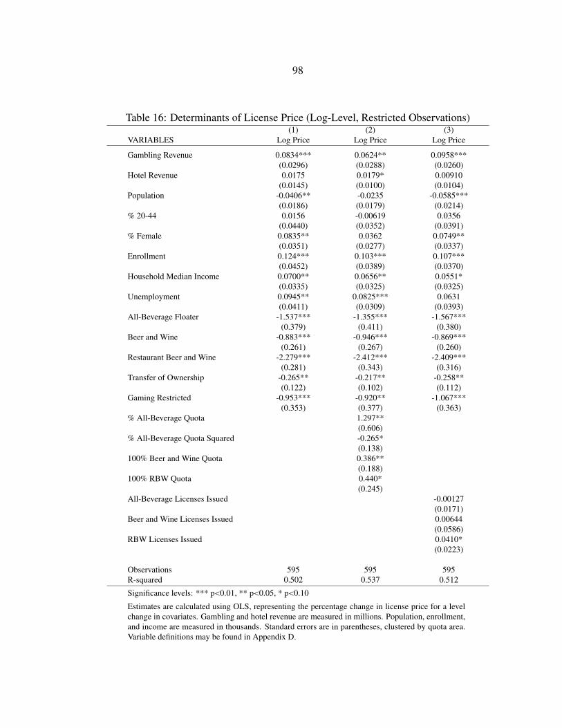
98
Table 16: Determinants of License Price (Log-Level, Restricted Observations)(1) (2) (3)
VARIABLES Log Price Log Price Log Price
Gambling Revenue 0.0834*** 0.0624** 0.0958***(0.0296) (0.0288) (0.0260)
Hotel Revenue 0.0175 0.0179* 0.00910(0.0145) (0.0100) (0.0104)
Population -0.0406** -0.0235 -0.0585***(0.0186) (0.0179) (0.0214)
% 20-44 0.0156 -0.00619 0.0356(0.0440) (0.0352) (0.0391)
% Female 0.0835** 0.0362 0.0749**(0.0351) (0.0277) (0.0337)
Enrollment 0.124*** 0.103*** 0.107***(0.0452) (0.0389) (0.0370)
Household Median Income 0.0700** 0.0656** 0.0551*(0.0335) (0.0325) (0.0325)
Unemployment 0.0945** 0.0825*** 0.0631(0.0411) (0.0309) (0.0393)
All-Beverage Floater -1.537*** -1.355*** -1.567***(0.379) (0.411) (0.380)
Beer and Wine -0.883*** -0.946*** -0.869***(0.261) (0.267) (0.260)
Restaurant Beer and Wine -2.279*** -2.412*** -2.409***(0.281) (0.343) (0.316)
Transfer of Ownership -0.265** -0.217** -0.258**(0.122) (0.102) (0.112)
Gaming Restricted -0.953*** -0.920** -1.067***(0.353) (0.377) (0.363)
% All-Beverage Quota 1.297**(0.606)
% All-Beverage Quota Squared -0.265*(0.138)
100% Beer and Wine Quota 0.386**(0.188)
100% RBW Quota 0.440*(0.245)
All-Beverage Licenses Issued -0.00127(0.0171)
Beer and Wine Licenses Issued 0.00644(0.0586)
RBW Licenses Issued 0.0410*(0.0223)
Observations 595 595 595R-squared 0.502 0.537 0.512
Significance levels: *** p<0.01, ** p<0.05, * p<0.10
Estimates are calculated using OLS, representing the percentage change in license price for a levelchange in covariates. Gambling and hotel revenue are measured in millions. Population, enrollment,and income are measured in thousands. Standard errors are in parentheses, clustered by quota area.Variable definitions may be found in Appendix D.
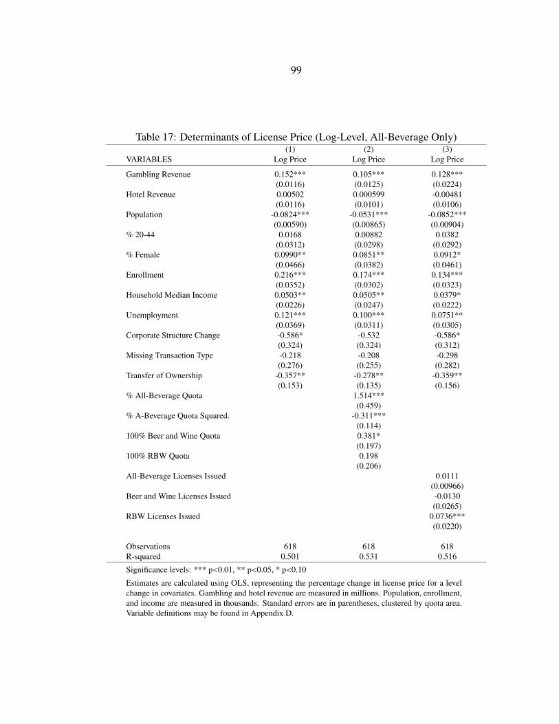
99
Table 17: Determinants of License Price (Log-Level, All-Beverage Only)(1) (2) (3)
VARIABLES Log Price Log Price Log Price
Gambling Revenue 0.152*** 0.105*** 0.128***(0.0116) (0.0125) (0.0224)
Hotel Revenue 0.00502 0.000599 -0.00481(0.0116) (0.0101) (0.0106)
Population -0.0824*** -0.0531*** -0.0852***(0.00590) (0.00865) (0.00904)
% 20-44 0.0168 0.00882 0.0382(0.0312) (0.0298) (0.0292)
% Female 0.0990** 0.0851** 0.0912*(0.0466) (0.0382) (0.0461)
Enrollment 0.216*** 0.174*** 0.134***(0.0352) (0.0302) (0.0323)
Household Median Income 0.0503** 0.0505** 0.0379*(0.0226) (0.0247) (0.0222)
Unemployment 0.121*** 0.100*** 0.0751**(0.0369) (0.0311) (0.0305)
Corporate Structure Change -0.586* -0.532 -0.586*(0.324) (0.324) (0.312)
Missing Transaction Type -0.218 -0.208 -0.298(0.276) (0.255) (0.282)
Transfer of Ownership -0.357** -0.278** -0.359**(0.153) (0.135) (0.156)
% All-Beverage Quota 1.514***(0.459)
% A-Beverage Quota Squared. -0.311***(0.114)
100% Beer and Wine Quota 0.381*(0.197)
100% RBW Quota 0.198(0.206)
All-Beverage Licenses Issued 0.0111(0.00966)
Beer and Wine Licenses Issued -0.0130(0.0265)
RBW Licenses Issued 0.0736***(0.0220)
Observations 618 618 618R-squared 0.501 0.531 0.516
Significance levels: *** p<0.01, ** p<0.05, * p<0.10
Estimates are calculated using OLS, representing the percentage change in license price for a levelchange in covariates. Gambling and hotel revenue are measured in millions. Population, enrollment,and income are measured in thousands. Standard errors are in parentheses, clustered by quota area.Variable definitions may be found in Appendix D.

100
Table 18: Determinants of License Price (Level-Level)(1) (2) (3)
VARIABLES Price Price Price
Gambling Revenue 10.86*** 9.710*** 15.89***(1.340) (1.054) (2.357)
Hotel Revenue 2.421** 1.910** 0.820(1.179) (0.788) (0.792)
Population -4.409*** -3.435*** -5.460***(0.728) (0.624) (1.214)
% 20-44 -4,012 -3,434 1,544(3,122) (2,386) (1,953)
% Female 5,492 2,958 4,774*(4,174) (3,003) (2,793)
Enrollment 21.48*** 18.39*** 19.48***(4.224) (3.997) (3.698)
Household Median Income. 7.722*** 6.232*** 4.311***(2.504) (2.042) (1.346)
Unemployment 9,049*** 6,962*** 3,738*(2,745) (2,568) (1,983)
All-Beverage Floater -192,473*** -190,992*** -204,565***(41,606) (41,961) (38,293)
Beer and Wine -56,455*** -60,842*** -48,987***(17,305) (17,663) (17,161)
Restaurant Beer and Wine -271,273*** -282,124*** -290,095***(52,258) (47,904) (51,635)
Corporate Structure Change -43,110* -41,539* -54,512***(22,608) (23,216) (19,985)
Missing Transaction Type -16,511 -23,689 -27,629(20,508) (18,715) (19,654)
Transfer of Ownership -21,606 -21,155* -26,888**(13,371) (12,200) (12,734)
Gaming Restricted -212,202*** -211,466*** -238,272***(48,713) (47,496) (50,074)
% All-Beverage Quota 59,250(39,343)
% All-Beverage Quota Squared. -18,144(11,446)
100% Beer and Wine Quota 22,862(17,351)
100% RBW Quota 40,718(28,222)
All-Beverage Licenses Issued 263.7(905.6)
Beer and Wine Licenses Issued -7,767***(2,499)
RBW Licenses Issued 8,225***(1,869)
Observations 892 892 892R-squared 0.590 0.608 0.625
Significance levels: *** p<0.01, ** p<0.05, * p<0.10
Estimates are calculated using OLS, representing the level change in license price for a level changein covariates. Gambling and hotel revenue are measured in thousands. Population, enrollment, andincome are measured in ones. Standard errors are in parentheses, clustered by quota area. Variabledefinitions may be found in Appendix D.

101
Table 19: Determinants of License Price (Log-Log)(1) (2) (3)
VARIABLES Log Price Log Price Log Price
Log Gambling Revenue 0.248*** 0.109** 0.168***(0.0826) (0.0429) (0.0582)
Log Hotel Revenue 0.142* 0.102 0.186***(0.0773) (0.0701) (0.0655)
Log Population -0.529*** -0.238** -0.180*(0.155) (0.117) (0.106)
% 20-44 -0.0162 -0.00871 -0.0319(0.0360) (0.0306) (0.0268)
% Female 0.0197 0.0333 -0.0638(0.0604) (0.0429) (0.0526)
Log Enrollment 0.269*** 0.197*** 0.119***(0.0643) (0.0518) (0.0453)
Log Household Median Income 2.354* 2.186** 0.898(1.257) (1.071) (0.789)
Unemployment 0.0735 0.0561* 0.0338(0.0452) (0.0306) (0.0343)
All-Beverage Floater -1.045*** -0.806* -1.313***(0.382) (0.442) (0.375)
Beer and Wine -0.568** -0.763*** -0.767***(0.245) (0.276) (0.225)
Restaurant Beer and Wine -1.930*** -2.231*** -2.312***(0.322) (0.328) (0.298)
Corporate Structure Change -0.460* -0.385 -0.368(0.242) (0.242) (0.228)
Missing Transaction Type -0.366 -0.307 -0.0916(0.292) (0.245) (0.247)
Transfer of Ownership -0.469*** -0.353*** -0.247**(0.155) (0.110) (0.120)
Gaming Restricted -0.699 -0.648 -1.166***(0.451) (0.417) (0.352)
% All-Beverage Quota 2.123***(0.511)
% All-Beverage Quota Squared -0.453***(0.144)
100% Beer and Wine Quota 0.444***(0.156)
100% RBW Quota 0.432*(0.219)
All-Beverage Licenses Issued -0.0502***(0.00644)
Beer and Wine Licenses Issued 0.109***(0.0150)
RBW Licenses Issued 0.0164(0.0127)
Observations 892 892 892R-squared 0.367 0.442 0.488
Significance levels: *** p<0.01, ** p<0.05, * p<0.10
Estimates are calculated using OLS, representing the percentage change in license price for a per-centage change in covariates. Gambling and hotel revenue are measured in millions. Population,enrollment, and income are measured in thousands. Standard errors are in parentheses, clustered byquota area. Variable definitions may be found in Appendix D.

102
Table 20: Determinants of License Price (Log-Level, Area & Year Fixed Effects)(1) (2) (3)
VARIABLES Log Price Log Price Log Price
Gambling Revenue 0.0173 0.0183 0.00786(0.0331) (0.0348) (0.0354)
Hotel Revenue 0.0425 0.0399 0.0489(0.0353) (0.0360) (0.0357)
Population -0.0722** -0.0598* -0.206***(0.0357) (0.0356) (0.0664)
% 20-44 0.0335 0.0494 0.0548(0.150) (0.153) (0.148)
% Female 0.0896 0.0833 0.0530(0.315) (0.323) (0.309)
Enrollment 0.101 0.0803 -0.0279(0.159) (0.156) (0.187)
Household Median Income 0.0156 0.0108 0.0148(0.0389) (0.0392) (0.0389)
Unemployment -0.00213 -0.00462 -0.00128(0.0765) (0.0777) (0.0688)
All-Beverage Floater -1.215*** -1.204*** -1.223***(0.401) (0.411) (0.406)
Beer and Wine -0.801*** -0.810*** -0.815***(0.286) (0.290) (0.286)
Restaurant Beer and Wine -2.575*** -2.570*** -2.591***(0.370) (0.391) (0.383)
Corporate Structure Change -0.360 -0.354 -0.350(0.304) (0.305) (0.300)
Missing Transaction Type -0.271 -0.270 -0.293(0.323) (0.318) (0.334)
Transfer of Ownership -0.200* -0.201* -0.202*(0.114) (0.113) (0.116)
Gaming Restricted -1.084*** -1.053*** -1.087***(0.376) (0.390) (0.388)
% All-Beverage Quota -0.0360(1.281)
% All-Beverage Quota Squared. 0.0222(0.235)
100% Beer and Wine Quota 0.121(0.171)
100% RBW Quota 0.288(0.363)
All-Beverage Licenses Issued 0.0389(0.0425)
Beer and Wine Licenses Issued 0.110**(0.0544)
RBW Licenses Issued 0.0325(0.0246)
Observations 892 892 892R-squared 0.640 0.641 0.641
Significance levels: *** p<0.01, ** p<0.05, * p<0.10
Estimates are calculated using OLS, representing the percentage change in license price for a levelchange in covariates. Gambling and hotel revenue are measured in millions. Population, enrollment,and income are measured in thousands. Standard errors are in parentheses, clustered by quota area.Variable definitions may be found in Appendix D.
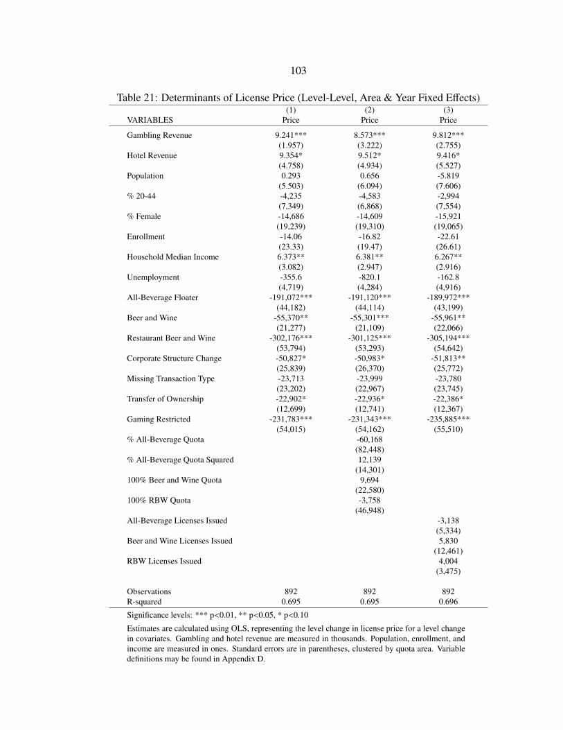
103
Table 21: Determinants of License Price (Level-Level, Area & Year Fixed Effects)(1) (2) (3)
VARIABLES Price Price Price
Gambling Revenue 9.241*** 8.573*** 9.812***(1.957) (3.222) (2.755)
Hotel Revenue 9.354* 9.512* 9.416*(4.758) (4.934) (5.527)
Population 0.293 0.656 -5.819(5.503) (6.094) (7.606)
% 20-44 -4,235 -4,583 -2,994(7,349) (6,868) (7,554)
% Female -14,686 -14,609 -15,921(19,239) (19,310) (19,065)
Enrollment -14.06 -16.82 -22.61(23.33) (19.47) (26.61)
Household Median Income 6.373** 6.381** 6.267**(3.082) (2.947) (2.916)
Unemployment -355.6 -820.1 -162.8(4,719) (4,284) (4,916)
All-Beverage Floater -191,072*** -191,120*** -189,972***(44,182) (44,114) (43,199)
Beer and Wine -55,370** -55,301*** -55,961**(21,277) (21,109) (22,066)
Restaurant Beer and Wine -302,176*** -301,125*** -305,194***(53,794) (53,293) (54,642)
Corporate Structure Change -50,827* -50,983* -51,813**(25,839) (26,370) (25,772)
Missing Transaction Type -23,713 -23,999 -23,780(23,202) (22,967) (23,745)
Transfer of Ownership -22,902* -22,936* -22,386*(12,699) (12,741) (12,367)
Gaming Restricted -231,783*** -231,343*** -235,885***(54,015) (54,162) (55,510)
% All-Beverage Quota -60,168(82,448)
% All-Beverage Quota Squared 12,139(14,301)
100% Beer and Wine Quota 9,694(22,580)
100% RBW Quota -3,758(46,948)
All-Beverage Licenses Issued -3,138(5,334)
Beer and Wine Licenses Issued 5,830(12,461)
RBW Licenses Issued 4,004(3,475)
Observations 892 892 892R-squared 0.695 0.695 0.696
Significance levels: *** p<0.01, ** p<0.05, * p<0.10
Estimates are calculated using OLS, representing the level change in license price for a level changein covariates. Gambling and hotel revenue are measured in thousands. Population, enrollment, andincome are measured in ones. Standard errors are in parentheses, clustered by quota area. Variabledefinitions may be found in Appendix D.

104
Table 22: Determinants of License Price (Log-Log, Area & Year Fixed Effects)(1) (2) (3)
VARIABLES Log Price Log Price Log Price
Log Gambling Revenue -0.0335 -0.0416 -0.0357(0.129) (0.127) (0.132)
Log Hotel Revenue 0.231 0.271 0.243(0.761) (0.768) (0.765)
Log Population -2.302* -2.207* -3.826*(1.322) (1.195) (2.073)
% 20-44 0.0470 0.0609 0.0680(0.187) (0.188) (0.187)
% Female 0.162 0.158 0.142(0.313) (0.318) (0.310)
Log Enrollment 0.232*** 0.201*** 0.224***(0.0488) (0.0492) (0.0529)
Log Household Median Income 0.852 0.586 0.935(1.369) (1.392) (1.409)
Unemployment 0.00549 -0.00287 0.0154(0.0826) (0.0829) (0.0851)
All-Beverage Floater -1.222*** -1.193*** -1.218***(0.421) (0.416) (0.426)
Beer and Wine -0.800*** -0.806*** -0.801***(0.285) (0.288) (0.286)
Restaurant Beer and Wine -2.553*** -2.537*** -2.547***(0.367) (0.392) (0.380)
Corporate Structure Change -0.373 -0.363 -0.372(0.303) (0.305) (0.306)
Missing Transaction Type -0.269 -0.271 -0.281(0.321) (0.316) (0.333)
Transfer of Ownership -0.197* -0.196* -0.200*(0.112) (0.111) (0.116)
Gaming Restricted -1.112*** -1.080*** -1.120***(0.370) (0.371) (0.392)
% All-Beverage Quota -0.0430(1.311)
% All-Beverage Quota Squared 0.0165(0.241)
100% Beer and Wine Quota 0.207(0.166)
100% RBW Quota 0.222(0.348)
All-Beverage Licenses Issued 0.0183(0.0422)
Beer and Wine Licenses Issued 0.0578(0.0582)
RBW Licenses Issued -0.00360(0.0185)
Observations 892 892 892R-squared 0.640 0.642 0.641
Significance levels: *** p<0.01, ** p<0.05, * p<0.10
Estimates are calculated using OLS, representing the percentage change in license price for a per-centage change in covariates. Gambling and hotel revenue are measured in millions. Population,enrollment, and income are measured in thousands. Standard errors are in parentheses, clustered byquota area. Variable definitions may be found in Appendix D.
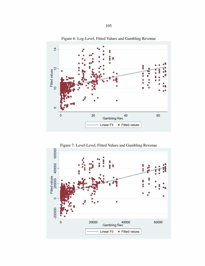
105
Figure 6: Log-Level, Fitted Values and Gambling Revenue
Figure 7: Level-Level, Fitted Values and Gambling Revenue

106
Figure 8: Log-Log, Fitted Values and Log Gambling Revenue
Figure 9: Log-Level, Fitted Values and Median Income
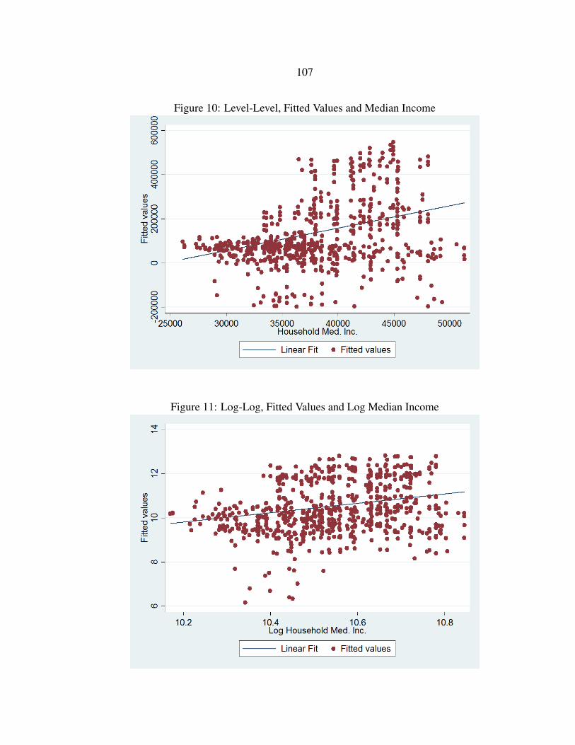
107
Figure 10: Level-Level, Fitted Values and Median Income
Figure 11: Log-Log, Fitted Values and Log Median Income

108
Figure 12: Log-Level, Fitted Values and Hotel Revenue
Figure 13: Level-Level, Fitted Values and Hotel Revenue
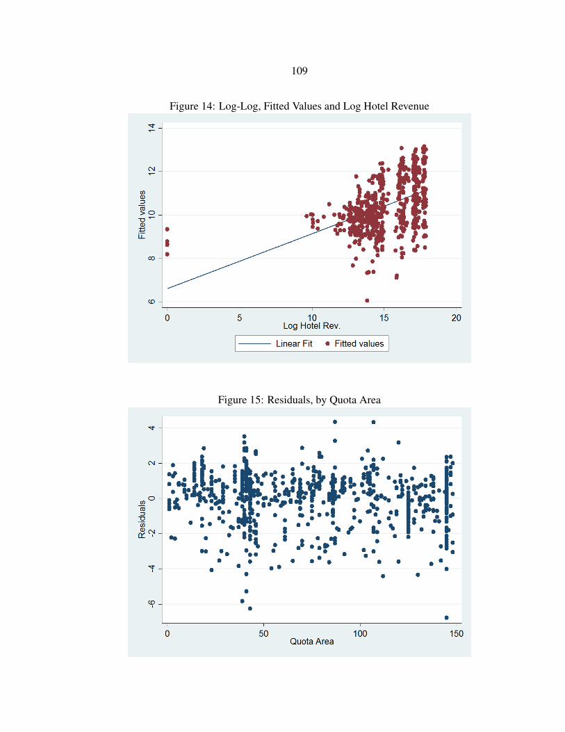
109
Figure 14: Log-Log, Fitted Values and Log Hotel Revenue
Figure 15: Residuals, by Quota Area
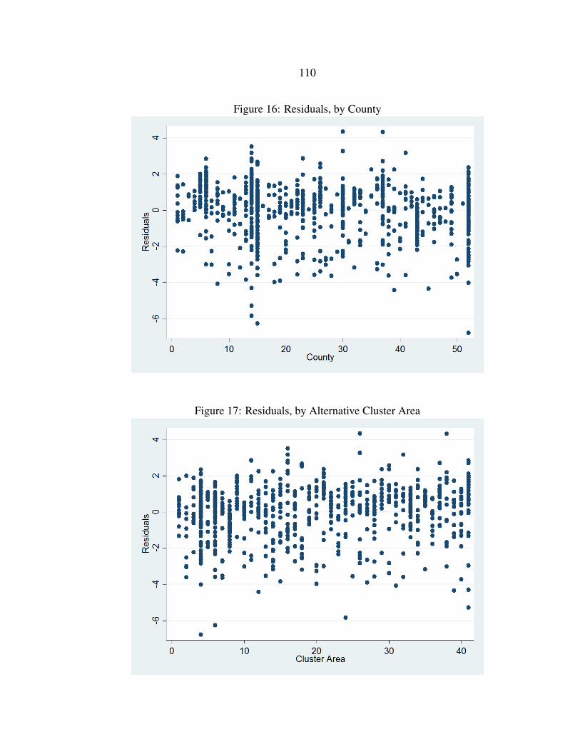
110
Figure 16: Residuals, by County
Figure 17: Residuals, by Alternative Cluster Area
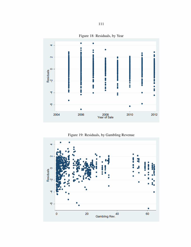
111
Figure 18: Residuals, by Year
Figure 19: Residuals, by Gambling Revenue

112
Figure 20: Residuals, by Income
Figure 21: Residuals, by Hotel Revenue

113
Table 23: Determinants of Licenses Issued(1) (2) (3)
VARIABLES AB Lic. Issued BW Lic. Issued RBW Lic. Issued
Gambling Revenue 0.000931** 0.00100*** 0.000105(0.000393) (0.000107) (0.000235)
Hotel Revenue -5.58e-05 3.57e-05 0.000132***(4.47e-05) (2.50e-05) (4.18e-05)
Population 0.679*** -0.0973** 0.212(0.0982) (0.0453) (0.159)
% 20-44 18.36 3.067 -20.49***(14.66) (4.494) (5.315)
% Female -26.35 -12.13* 4.222(18.08) (6.751) (6.939)
Enrollment -0.498 0.620*** 0.349(0.549) (0.186) (0.268)
Household Median Income -0.0481 -0.0471* 0.0855***(0.0792) (0.0264) (0.0315)
Unemployment 0.206** 0.0672* 0.299***(0.103) (0.0393) (0.0706)
Unincorporated -0.749 -1.086**(1.321) (0.418)
Constant 12.38 7.487* -1.572(10.65) (3.882) (3.642)
Observations 1,472 1,472 1,024R-squared 0.849 0.911 0.801
Significance levels: *** p<0.01, ** p<0.05, * p<0.10
Estimates are calculated using OLS, representing the level change in license number for a levelchange in covariates. Gambling and hotel revenue are measured in thousands. Population, enroll-ment, and income are measured in ones. Standard errors are in parentheses, clustered by quotaarea. Column 1 considers all-beverage licenses issued; Columns 2 and 3 consider beer and wineand restaurant beer and wine licenses issued, respectively. RBW licenses are only issued in incor-porated areas, hence the lower observation count.

114
Table 24: Determinants of Licenses Issued (Area Fixed Effects)(1) (2) (3)
VARIABLES AB Lic. Issued BW Lic. Issued RBW Lic. Issued
Gambling Revenue -1.18e-05 9.10e-05*** -8.65e-05(5.59e-05) (2.90e-05) (0.000123)
Hotel Revenue -4.25e-05 -1.92e-05 0.000153**(2.79e-05) (1.68e-05) (6.92e-05)
Population 0.957*** 0.460*** 0.636***(0.0437) (0.0344) (0.0839)
% 20-44 0.927 -1.066 -2.449(2.005) (1.083) (3.275)
% Female 6.016 3.613 8.566(6.200) (2.457) (5.744)
Enrollment 0.150 0.262 3.364***(0.685) (0.378) (0.540)
Household Median Income -0.0193* -0.00973** -0.0258(0.0107) (0.00409) (0.0186)
Unemployment 0.0222 -0.0181* 0.180***(0.0205) (0.00982) (0.0519)
Unincorporated -25.36*** -19.84***(2.113) (1.267)
Constant 7.874** 2.559** -8.333***(3.062) (1.063) (3.163)
Observations 1,472 1,472 1,024R-squared 0.999 0.999 0.976
Significance levels: *** p<0.01, ** p<0.05, * p<0.10
Estimates are calculated using OLS, representing the level change in license number for a levelchange in covariates. Gambling and hotel revenue are measured in thousands. Population, enroll-ment, and income are measured in ones. Standard errors are in parentheses, clustered by quotaarea. Column 1 considers all-beverage licenses issued; Columns 2 and 3 consider beer and wineand restaurant beer and wine licenses issued, respectively. RBW licenses are only issued in incor-porated areas, hence the lower observation count.

115
CONCLUSION AND DISCUSSION
Implications of the Study
This study both lays out a theoretical model for tradable licenses to operate and
empirically tests the implications that the model yields. The effect of positive demand
shifters, particularly, appear to be significant determinants of license values. Gambling,
income, university enrollment, and, to a lesser extent, tourism (using hotel revenue as a
proxy) all are statistically and economically significant predictors of license price. These
results, moreover, are robust to the inclusion of supply variables, and robust to alternative
functional forms. Thus, the empirical analysis provides a great deal of support for the
demand-side predictions of the model.
The most consistent determinants of license prices, however, are the attributes of
an individual license. License type, along with whether or not a license carries the right to
gamble, are strong predictors of how much a license is worth on the market. Even more so
than the continuous demand variables, indicator variables for license attributes are robust
to different specifications. The qualitative and quantitative estimated effects remain
consistent when supply variables are added, and are extremely robust to different
functional forms. Even more noteworthy is the robustness of the variables to the inclusion
of fixed effects, which conditioned out most of the identifying variation in the data. Again,
these empirical results support the predictions produced by theory.
The estimated magnitudes of the effects, however, should be treated with caution.
Although licenses issued in a quota system typically are thought of as exogenous, the

116
quotas in Montana’s licensing system are not always firm. Many areas are allowed to be
over quota, occasionally by a wide margin (e.g., Butte has three times the licenses
permitted by their quota). The robustness of the results, however, mitigates some of the
concerns over endogeneity bias. Similarly, the analysis is descriptive—the estimates
provide predictive information, as opposed to strictly causal effects. Given the infrequency
with which licenses trade, however, the large-scale cross-sectional differences in the data
probably still provide a good deal of insight into why licenses are priced as they are.
While the empirical analysis supports the predictions regarding the demand-side
determinants in the model, the results do not provide much evidence supporting the
prediction regarding changes in quota. The model predicts that an increase in quota should
lead to lower prices, provided the quota is binding. Unfortunately, the particulars of the
Montana alcohol licensing system do not provide many opportunities to cleanly test the
implication. Montana expanded the RBW license quota in 2007, but several factors
preclude a simple analysis of the impacts of the change. the analysis. First, many areas
had non-binding quotas to begin with, which negates the prediction. Second, the areas
with binding quotas adjusted relatively slowly to the increase in available licenses.79
Additionally, all-beverage floater licenses do not provide a clean way to evaluate
the prediction. While the licenses float to an area with high license demand, both locations
involved in the transaction are definitionally over quota. If the buyer’s area was not over
100 percent of the allowable licenses, a new license could be issued by the department.
Both markets involved, moreover, typically see only marginal changes in the supply of
79It is not easy to tell whether this was due to an overall lack of interest in the new RBW licenses, or dueto time lags in the application approval process, or a combination thereof.

117
licenses. If licenses float out of Butte and into Billings, neither location sees a large
relative change in supply. Again, this makes it difficult to identify the effect of a change in
the number of licenses.
Although the implications surrounding changes to the number of licenses are not
effectively tested, the analysis is still the first to explicitly lay out and test the model’s
predictions in the context of alcohol retail licensure. The results also provide evidence that
the model is an appropriate way think about Montana’s licensing system, particularly for
the demand-side determinants of price. Thus, a clear contribution is made to the
economics of alcohol literature particularly, and to the business licensure literature more
generally. The results, moreover, provide insight into several policy changes. For
example, the estimated discount for restricted gambling rights provides a quantitative
result that may be used to evaluate the effects of the 1997 and 2007 restrictions on
gambling (for incorporated beer and wine and floater licenses, respectively). Given how
involved the Montana state government is in the retail alcohol industry, the analysis
provides valuable information regarding future policy discussion.
Possibilities for Future Analysis
While examining the price determinants of Montana’s alcohol retail licenses
provides a clear addition to the literature, the licensing system provides several other
avenues for future research. In particular, the rents created by the system lend themselves
well to economic analysis. While getting at the value of the total rents within certain quota
areas is relatively straightforward (i.e., multiply the average license price by the number of

118
licenses active in a quota area), it is more difficult to get at the total value state-wide.
Using the results of the model, values may be imputed for the areas that are more thinly
traded. This analysis would also provide insight into what would occur if licenses could
trade freely across quota areas. Licenses would move to the higher-priced areas, until
rents were equal across the different markets.
Similarly, an interesting issue is how rents have changed over time. When the
system was instituted in 1947, the state grandfathered existing establishments. At that
point, license prices and rents were probably close to zero.80 Between the inception of the
quota program and now, rents appear to have increased a great deal (at least in nominal
terms). Thus, it appears that the adjustment factor in licenses in incorporated areas (one
additional all-beverage license per 1,500 people after a certain threshold) is not sufficient
to keep up with the increase in demand. In incorporated communities, licenses have
substantial value. In unincorporated areas, however, the increase in licenses associated
with population growth (one license per 750 people) appears to out-pace the growth in
demand. In many counties (the larger counties population-wise in particular), license
values are quite close to zero.
Another testable implication of the model consists of the increase in quantity
supplied by each establishment. With the introduction of a binding quota, the number of
operating businesses declines. Each licensed establishment, however, increases their own
quantity supplied (from qi to q′i in figure 2, above). Thus, areas with binding quotas are
expected to see increased quantity supplied for each establishment—this could take the
80Rents were not necessarily zero with the inception of the program. If population growth was expected,capping the number of bars may have increased expected future profit.

119
form of increased seating or increased floorspace. The effect on both margins could
conceivably be tested empirically.
Two other issues also lend themselves well to analysis. Market liquidity, for
example, is another pertinent issue, particularly for those concerned with issuing loans
with a license as collateral. In the event of a default, whoever assumes ownership of the
license (on non-use status) must sell it within 180 days.81 Thus, the ease with which a
license may be transferred is of paramount importance if they are used as collateral. Using
the proportion of licenses traded by quota area/year as the dependent variable, various
factors could be used to predict when licenses change hands.
The second potential area of interest is lottery system in place to allocate new
licenses. This literature is well developed, particularly in resource economics (relating to
hunting permits), but not in the area of retail licenses. Additionally, Montana has made
several large changes to the entry requirements for license lotteries. For example, the state
increased the credit requirement in 2007. Potentially, this should lower the number of
applicants, as the costs to enter the lottery are higher. Similarly, there is the issue of the
preferential lottery with RBW licenses, as well as recently instituted holding periods.
Although examining the determinants of license prices provides significant insight
into the licensing system in Montana, there are still a plethora of other questions that could
be addressed. Given the complexities of the system, there are deep economic implications
in the way the state deals with licensing alcoholic beverage retailers. Similarly, there are a
host of other economically relevant topics surrounding wholesalers and manufacturers.
81See M.C.A. 16-4-801.

120
REFERENCES CITED
121
Administrative Rules of Montana. (2013). Chapter 42.12: Liquor Licenses and Permits.
Buschena, David E., Anderson, Terry L., and Leonard, Jerry L. (2001). ValuingNon-Marketed Goods: The Case of Elk Permit Lotteries. Journal of EnvironmentalEconomics and Management, 41: 33-43.
Cairns, Robert D., and Liston-Heyes, Catherine. (1996). Competition and Regulation inthe Taxi Industry. Journal of Public Economics, 59(1): 1-15.
Carpenter, Christopher S. (2007). Heavy Alcohol Use and Crime: Evidence fromUnderage Drunk-Driving Laws. Journal of Law and Economics, 50(3): 539-557.
Carpenter, Christopher S., and Eisenberg, Daniel. (2009). Effects of Sunday SalesRestrictions on Overall and Day-Specific Alcohol Consumption: Evidence fromCanada. Journal of Studies on Alcohol an Drugs, 70(1): 126-133.
Congressional Research Service. (2004). The Constitution of the United States ofAmerica: Analysis and Interpretation. George A. Costello, Johnny H. Killian, andKenneth R. Thomas (Eds.). Washington, DC: U.S. Government Printing Office.
Cook, Phillip J., and Tuachen, George. (1982). The Effect of Liquor Taxes on HeavyDrinking. The Bell Journal of Economics, 13(2): 379-390.
Cook, Philip J., Ostermann, Jan, and Sloan, Frank A. (2005). Are Alcohol Excise TaxesGood for Us? Short and Long-Term Effects on Mortality Rates. NBER Working Paper11138.
Cooper, James C., and Wright, Joshua D. (2012). Alcohol, Antitrust, and the 21stAmendment: An Empirical Examination of Post and Hold Laws. International Reviewof Law and Economics, 32(4): 379-392.
Crocker, Thomas D. (1966). The Structuring of Atmospheric Pollution Control Systems.The Economics of Air Pollution, 61-86. Ed. Harold Wolozin. New York: Norton.
Dales, J. H. (1968). Pollution, Property, and Prices. Toronto: University of Toronto Press.
Demsetz, Harold. (1982). Barriers to Entry. American Economic Review, 72(1): 47-57.
Halvorsen, Robert and Palmquist, Raymond. (1980). The Interpretation of DummyVariables in Semilogarithmic Equations. The American Economic Review, 70(3):474-475.
Harrison, Melynda. (2011). Local Knowledge: The Spirit of Montana. Big Sky Journal,Arts 2011. Retrieved from http://www.bigskyjournal.com/articles/big-sky-journal/arts-2011/136/local-knowledge-the-spirit-of-montana.html
122
Heaton, Paul. (2012). Sunday Liquor Laws and Crime. Journal of Public Economics,96(1): 42-52.
Hyman, David N. (1986). Modern Microeconomics: Analysis and Applications. (5th ed.,pp. 340-341). St. Louis, MO: Times Mirror/Mosby College Pub.
Lovenheim, Michael F., and Steffel, Daniel P. (2011). Do Blue Laws Save Lives? TheEffect of Sunday Alcohol Sales Bans on Fatal Vehicle Accidents. Journal of PolicyAnalysis and Management, 30(4): 798-820.
Markowitz, Sara. (2005). Alcohol, Drugs, and Violent Crime. International Review ofLaw and Economics, 25(1): 20-44.
McMillan, Garnett P., and Lapham, Sandra. (2006). Legalized Sunday Packaged AlcoholSales and Alcohol-Related Traffic Crashes and Crash Fatalities in New Mexico.American Journal of Public Health, 96(11): 1944-1948.
Miron, Jeffrey A., and Tetelbaum, Elina. (2009). Does the Minimum Legal Drinking AgeSave Lives? Economic Inquiry, 47(2): 317-336.
Montana Code Annotated. (2013). Title 16: Alcohol and Tobacco.
Montana Code Annotated. (2013). Title 23: Parks, Recreation, Sports, and Gambling.
Montana Department of Health & Human Services. (2009). Talking about the MontanaClean Indoor Air Act. Retrieved from http://www.dphhs.mt.gov/mtupp//cleanairact/talkingaboutciaa.pdf
Montana Department of Justice. (2005). McGrath: State will Not Appeal Liquor-LicenseDecision. Retrieved from https://doj.mt.gov/2005/06/mcgrath-state-will-not-appeal-liquor-license-decision/
Montana Department of Justice. (2013). History of Gambling in Montana. Retrieved fromhttps://doj.mt.gov/gaming/history-of-gambling/
Montana Department of Revenue. (2012). About Liquor Distribution in Montana.Retrieved from http://revenue.mt.gov/forbusinesses/alcohol beverage control/Liquor Store Agents and Vendors/learnaboutliquordistribution.mcpx
Montana Legislature: Revenue Oversight Committee. (1980). Montana’s Liquor LicenseQuota System: A Report to the Forty-Seventh Legislature. Helena, MT: MontanaLegislative Council.

123
Montana Legislature: Subcommittee on Judiciary. (1974). Alcoholic Beverage ControlStatutes: Interim Study. Helena, MT: Montana Legislative Council
Newhouse, Ryan. (2013). Montana Beer: A guide to Breweries in Big Sky Country.Charleston, SC: American Palate.
New York City Taxi & Limousine Commission. (2014). 2013 Monthly Medallions“Non-Accessible” Sales-Average Prices & Number of Transfers. Retrieved fromhttp://www.nyc.gov/html/tlc/downloads/pdf/avg med price 2013 december.pdf
Nickerson, Peter H. (1990). Demand for the Regulation of Recreation: The Case of Elkand Deer Hunting in Washington State. Land Economics, 66(4): 437-447.
Quinn, Larry D. (1970). Politicians in Business: A History of the Liquor Control Systemin Montana. Missoula, MT: University of Montana Press.
Revised Code of Montana. (1967). Title 4: Alcoholic Beverages.
Rucker, Randal R., Thurman, Walter N., and Sumner, Daniel A. (1995). Restricting theMarket for Quota: An Analysis of Tobacco Production Rights with Corroborationfrom Congressional Testimony. Journal of Political Economy, 103(1): 142-175.
Saffer, Henry, and Dave, Dhaval. (2002). Alcohol Consumption and Alcohol AdvertisingBans. Applied Economics, 34(11): 1325-1334.
Sass, Tim R., and Saurman, David S. (1993). Mandated Exclusive Territories andEconomic Efficiency: An Empirical Analysis of The Malt Beverage Industry. Journalof Law and Economics, 36(1): 153-177.
Scrogin, David, Berrens, Robert P., and Bohara, Alok K. (2000). Policy Changes and theDemand for Lottery-Rationed Big Game Hunting Licenses. Journal of Agriculturaland Resource Economics, 25(2): 501-519.
Seim, Katja and Waldfogel, Joel. (2013). Public Monopoly and Economic Efficiency:Evidence from the Pennsylvania Liquor Control Board’s Entry Decisions. AmericanEconomic Review, 103(2): 831-862.
Silberberg, Eugene, and Suen, Wing. (2011).The Structure of Economics: A MathematicalAnalysis. (3rd ed., Revised). New York, NY: McGraw Hill.
Smith, Janet K. (1982). An Analysis of State Regulations Governing Liquor StoreLicensees. Journal of Law and Economics, 25 (2): 301-319.
Toma, Eugenia F. (1988). State Liquor Licensing, Implicit Contracting, and Dry/WetCounties. Economic Inquiry, 26(3): 507-524.

124
Tullock, Gordon. (1975). The Transitional Gains Gap. The Bell Journal of Economics,6(2): 671-678.
Tremblay, Victor J., and Okuyama, Kumiko. (2001). Advertising Restrictions,Competition, and Alcohol Consumption. Contemporary Economic Policy, 19(3):313-321.
Varian, Hal R. (1984.) Microeconomic Analysis. (2nd Ed. ). New York, NY: W. W.Norton & Company, Inc.
Wooldridge, Jeffrey M. (2009). Introductory Econometrics: A Modern Approach. (4thed.). Mason, OH: South-Western Cengage Learning.

125
APPENDICES
126
APPENDIX A
TIMELINE

127
Figure 22: Timeline of MT Alcohol Laws1930
1940
1950
1960
1970
1980
1990
2000
2010
1933 End of Prohibition; MT Liquor Control Board created; beer by-the-drink legalized
1937 Liquor by-the-drink legalized
1947 Incorporated license quota system created
1963 Unincorporated license quota implemented
1967 Beer off-premise sales legalized (year?)
1973 Department of Revenue assumes the MLCB’s duties1974 Wine amendment added to beer retail licenses1975 All-beverage, floater, and resort licenses created1976 MT Supreme Court legalizes video keno
1978 Voter initiative legalizes wine sales in grocery stores1979 Catering endorsements and airport licenses created
1984 MT Supreme Court rules video poker is illegal1985 Video Poker Machine Act allows 5 video poker machines per licensee
1987 15% income tax implemented on gambling machines
1991 Licensees limited to 20 total machines per licensed premises
1995 State liquor stores privatized
1997 Restaurant beer and wine licenses created
2005 U.S. District Court rules resident requirement unconsitutional
2007 Floaters gaming-restricted, RBW licenses doubled
2009 Smoking ban in effect

128
APPENDIX B
QUOTA FORMULAS

129
Table 25: All-Beverage Quota FormulaPopulation Quota
Less than 500 2 total
500 - 3,000 3 for the first 1,000; 1 for each additional 1,000
Greater than 3,000 5 for the first 3,000; 1 for each additional 1,500
Unincorporated 1 per 750
Table 26: Beer and Wine Quota FormulaPopulation Beer and Wine License Quota:
Less than 500 1 total
500 - 2,000 1 per 500
Greater than 2,000 4 for the first 2,000; 2 for the next 2,000; 1 for each additional 2,000
Unincorporated Subject to Department Discretion
Table 27: Restaurant Beer and Wine Quota FormulaPopulation: License Quota
Less than 5,000 80% of Beer Retail Quota; 1-time adjustment of +4 if quota is met
5000-20,000 160% of Beer Retail Quota
20,000-60,000 100% of Beer Retail Quota
Greater than 60,000 80% of Beer Retail Quota
Unincorporated None
Resort Community 200% of Beer Retail Quota
Table 28: Resort All-Beverage Quota FormulaPopulation: Quota
N/A 1 for the first 100 accomodation units; 1 for each additional 50
130
APPENDIX C
COMPARATIVE STATICS RESULTS

131
The two-identity system in equilibrium:
S (p∗B(L,α,β), L,α) ≡ D(p∗B(L,α,β),β)
L ≡ L(p∗L(L,α,β), p∗B(L,α,β))
Differentiating the system with respect to β1 to find the comparative statics results
associated with a positive demand shifter: :
∂S (·)∂p∗B(·)
·∂p∗B(·)∂β1
=∂D(·)∂p∗B(·)
·∂p∗B(·)∂β1
+∂D(·)∂β1
0 =∂L(·)∂p∗L(·)
·∂p∗L(·)∂β1
+∂L(·)∂p∗B(·)
·∂p∗B(·)∂β1
Rearranging and putting it into matrix notation:
(∂S (·)∂p∗B(·) −
∂D(·)∂p∗B(·)
)0
∂L(·)∂p∗B(·)
∂L(·)∂p∗L(·)
∂p∗B(·)∂β1
∂p∗L(·)∂β1
=
∂D(·)∂β1
0
Using Cramer’s Rule to solve for ∂p∗B(·)
∂β1:
∂p∗B(·)∂β1
=
∣∣∣∣∣∣∣∣∣∣∣∂D(·)∂β1
0
0 ∂L(·)∂p∗L(·)
∣∣∣∣∣∣∣∣∣∣∣∣∣∣∣∣∣∣∣∣∣∣(∂S (·)∂p∗B(·) −
∂D(·)∂p∗B(·)
)0
∂L(·)∂p∗B(·)
∂L(·)∂p∗L(·)
∣∣∣∣∣∣∣∣∣∣∣=
∂D(·)∂β1·∂L(·)∂p∗L(·)(
∂S (·)∂p∗B(·) −
∂D(·)∂p∗B(·)
)·∂L(·)∂p∗L(·)
Assuming that supply has an upward slope and demand a downward slope in the retail
market, ∂p∗B(·)β1
> 0.

132
Using Cramer’s Rule to solve for ∂p∗L(·)∂β1
:
∂p∗L(·)∂β1
=
∣∣∣∣∣∣∣∣∣∣∣(∂S (·)∂p∗B(·) −
∂D(·)∂p∗B(·)
)∂D(·)∂p∗B(·)
∂L(·)∂p∗B(·) 0
∣∣∣∣∣∣∣∣∣∣∣∣∣∣∣∣∣∣∣∣∣∣(∂S (·)∂p∗B(·) −
∂D(·)∂β1
)0
∂L(·)∂p∗B(·)
∂L(·)∂p∗L(·)
∣∣∣∣∣∣∣∣∣∣∣=
−∂D(·)∂β1·∂L(·)∂p∗B(·)(
∂S (·)∂p∗B(·) −
∂D(·)∂p∗B(·)
)·∂L(·)∂p∗L(·)
Assuming that supply has an upward slope and demand a downward slope in the retail
market, and demand has a downward slope in the license market, ∂p∗L(·)∂β1
> 0.
Differentiating the two-identity system with respect to L to find the comparative statics
results associated with a change in quota:
∂S (·)∂p∗B(·)
·∂p∗B(·)∂L
+∂S (·)∂L
=∂D(·)∂p∗B(·)
·∂p∗B(·)∂L
1 =∂L(·)∂p∗B(·)
·∂p∗B(·)∂L
+∂L(·)∂p∗L(·)
·∂p∗L(·)∂L
Rearranging and putting it into matrix notation:
(∂D(·)∂p∗B(·) −
∂S (·)∂p∗B(·)
)0
∂L(·)∂p∗B(·)
∂L(·)∂p∗L(·)
∂p∗B(·)∂L
∂p∗L(·)∂L
=
∂S (·)∂L
1
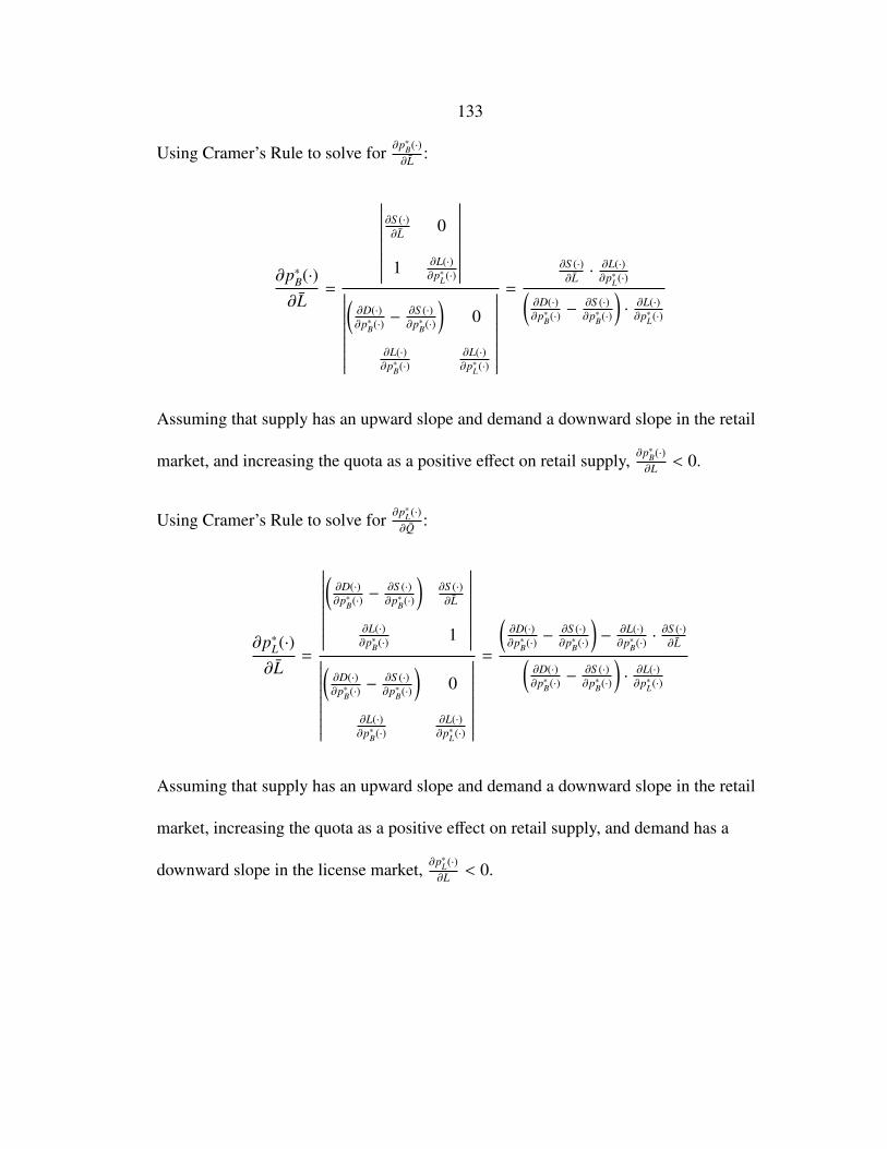
133
Using Cramer’s Rule to solve for ∂p∗B(·)∂L :
∂p∗B(·)∂L
=
∣∣∣∣∣∣∣∣∣∣∣∂S (·)∂L 0
1 ∂L(·)∂p∗L(·)
∣∣∣∣∣∣∣∣∣∣∣∣∣∣∣∣∣∣∣∣∣∣(∂D(·)∂p∗B(·) −
∂S (·)∂p∗B(·)
)0
∂L(·)∂p∗B(·)
∂L(·)∂p∗L(·)
∣∣∣∣∣∣∣∣∣∣∣=
∂S (·)∂L ·
∂L(·)∂p∗L(·)(
∂D(·)∂p∗B(·) −
∂S (·)∂p∗B(·)
)·∂L(·)∂p∗L(·)
Assuming that supply has an upward slope and demand a downward slope in the retail
market, and increasing the quota as a positive effect on retail supply, ∂p∗B(·)∂L < 0.
Using Cramer’s Rule to solve for ∂p∗L(·)∂Q :
∂p∗L(·)∂L
=
∣∣∣∣∣∣∣∣∣∣∣(∂D(·)∂p∗B(·) −
∂S (·)∂p∗B(·)
)∂S (·)∂L
∂L(·)∂p∗B(·) 1
∣∣∣∣∣∣∣∣∣∣∣∣∣∣∣∣∣∣∣∣∣∣(∂D(·)∂p∗B(·) −
∂S (·)∂p∗B(·)
)0
∂L(·)∂p∗B(·)
∂L(·)∂p∗L(·)
∣∣∣∣∣∣∣∣∣∣∣=
(∂D(·)∂p∗B(·) −
∂S (·)∂p∗B(·)
)−
∂L(·)∂p∗B(·) ·
∂S (·)∂L(
∂D(·)∂p∗B(·) −
∂S (·)∂p∗B(·)
)·∂L(·)∂p∗L(·)
Assuming that supply has an upward slope and demand a downward slope in the retail
market, increasing the quota as a positive effect on retail supply, and demand has a
downward slope in the license market, ∂p∗L(·)∂L < 0.
134
APPENDIX D
VARIABLE DEFINITIONS

135
Table 29: Variable DefinitionsVARIABLE DEFINITION
Gambling Revenue Gambling revenue, equal to gambling tax revenue over 0.15.Specified in millions with log-prices and in thousands with level.
Hotel Revenue Hotel revenue, equal to hotel tax revenue over 0.07. Specified inmillions with log-prices and in thousands with level.
Population Estimated annual population. Specified in thousands with log-pricesand in ones with level.
% 20-44 Estimated proportion of the county population ages 20 and 44.
% Female Estimated proportion of the county population that is female.
Enrollment Annual fall enrollment for all two and four year institutions.
Household Median Income Estimated annual household median income by county.
Unemployment Estimated annual unemployment by county.
All-Beverage Indicator variable for an all-beverage licenses (omitted).
All-Beverage Floater Indicator variable for an all-beverage floater license.
Beer and Wine Indicator variable for a beer/beer and wine retail license.
Restaurant Beer and Wine Indicator variable for a restaurant beer and wine license.
Corporate Structure Change Indicator variable for a corporate structure change.
Missing Transaction Type Indicator variable for a missing transaction type.
Transfer of Ownership Indicator variable for a transfer of ownership.
Transfer of Ownership & Location Indicator variable for a transfer of ownership and location (omitted).
Gaming Restricted Indicator variable for a license classified as gaming restricted.Takes on a value of 1 for gaming restricted all-beverage, floater,and beer and wine retail licenses.
% All-Beverage Quota Percentage of a quota area’s all-beverage quota, defined as licensesissued over license quota.
% All-Beverage Quota Squared Percentage of all-beverage quota squared.
100% BW Quota Indicator variable for a quota area being at or above the BW quota.
100% RBW Quota Indicator variable for a quota area bineg at or above the RBW quota.
All-Beverage Licenses Issued The numer of all-beverage licenses (including resort and floaterlicenses) issued in a quota area.
Beer and Wine Licenses Issued The number of beer and wine retail licenses issued in a quota area.
RBW Licenses Issued The number of RBW licenses issued in a quota area.

136
APPENDIX E
ALTERNATIVE CLUSTERS

137
Table 30: Alternative ClustersLocation(s) ObservationsBillings 92Butte 61Bozeman/Belgrade 59Missoula (City) 48Whitefish 30Great Falls 29Flathead, Uninc.† 28Park Co. 27Helena 21Kalispell 21Ravalli, Inc. 21Carbon Co. 20Fallon/Garfield/McCone/Powder River/Rosebud/Treasure Cos. 20Cascade/Chouteau/Judith Basin Cos.* 19Daniels/Sheridan/Roosevelt Cos. 19Valley Co. 19Gallatin, Inc.* 18Dawson/Richland/Wibaux Cos. 17Fergus Co. 17Licoln Co. 17Broadwater/Meagher/Wheatland Cos. 16Big Horn/Musselshell/Yellowstone, Cos.* 16Glacier/Toole Cos. 16Lake/Missoula, Uninc.† 16Blaine/Phillips Cos. 15Gallatin, Uninc.† 15Granite/Powell Co. 15Mineral/Sanders Cos. 15Jefferson Co. 14Pondera/Teton Cos. 14Beaverhead Co. 13Hill/Liberty Cos. 13Cascade/Lewis & Clark, Uninc.† 13Lake, Inc. 13Madison, Inc. 13Madison, Uninc. 13Ravalli, Uninc.† 13Anaconda 12Miles City 12Stillwater/Sweet Grass Cos. 12Big Horn/Dawson/Richland/Yellowstone, Uninc.† 10†Denotes the area(s) is under quota by more than 1 license.*The observation counts for Cascade, Gallatin, Big Horn, and Yellowstonecounties are compiled after other areas listed have been removed.Inc., Uninc, and Cos. refer to incorporated, unincorporated, and totalcounty areas, respectively.