1

AN ASSIGNMENT FREE DATA DRIVEN APPROACH TO THE DYNAMIC ORIGIN DESTINATION MATRIX ESTIMATION PROBLEM

X. Ros-Rocaa,b, J. Barcelóa,b, L. Monteroa, aDepartment of Statistics and Operations Research, Universitat Politècnica de Catalunya bPTV GROUP Abstract Dynamic traffic models require dynamic inputs, and one of the main inputs are the Dynamic Origin-Destinations (OD) matrices describing the variability over time of the trip patterns across the network. The Dynamic OD Matrix Estimation (DODME) is a hard problem since no direct full observations are available, and therefore one should resort to indirect estimation approaches. Among the most efficient approaches, the one that formulates the problem in terms of a bilevel optimization problem has been widely used. This formulation solves at the upper level a nonlinear optimization that minimizes some distance measures between observed and estimated link flow counts at certain counting stations located in a subset of links in the network, and at the lower level a traffic assignment that estimates these link flow counts assigning the current estimated matrix. The variants of this formulation differ in the analytical approaches that estimate the link flows in terms of the assignment and their time dependencies. Since these estimations are based on a traffic assignment at the lower level, these analytical approaches, although numerically efficient, imply a high computational cost. The advent of ICT applications has made available new sets of traffic related measurements enabling new approaches; under certain conditions, the data collected on used paths could be interpreted as an empirical assignment observed de facto. This allows extracting empirically the same information provided by an assignment that is used in the analytical approaches. This research report explores how to extract such information from the recorded data, proposes a new optimization model to solve the DODME problem, and computational results on its performance. Key Words: Dynamic OD Estimation, Bi-level Optimization, Non-linear optimization, ICT Data 1. Introduction: Analytical Approaches to DODME

Trip patterns in terms of Origin to Destination (OD) traffic flows are a key input to traffic assignment models, namely to Dynamic Traffic Assignment models, where they also must be dynamic, or at least time discretized, to properly approximate the time variability of the demand. OD matrices are not yet observable; in the best case, the measurements from Information and Communication Technologies (ICT), as GPS vehicle tracking, or mobile phones Call Detail Records (CDR), allow drawing samples that must be suitably expanded to provide estimates of the whole population. Therefore, their estimation must be done resorting to indirect process, usually based on mathematical models.

One of the most appealing mathematical formulations of the OD estimation problem is in terms of bilevel optimization problems (1), aimed at adjusting an initial target OD, 𝑿𝑿𝑯𝑯, so that it could explain the observed link flow counts 𝒀𝒀� at counting stations in the network, Ros-Roca et al. (2018).

𝑚𝑚𝑚𝑚𝑚𝑚 𝑍𝑍(𝑿𝑿,𝒀𝒀) = 𝑤𝑤1𝐹𝐹1�𝑿𝑿,𝑿𝑿𝑯𝑯�+ 𝑤𝑤2𝐹𝐹2�𝒀𝒀,𝒀𝒀�� (1)

𝒀𝒀 = 𝐴𝐴𝐴𝐴𝐴𝐴𝑚𝑚𝐴𝐴𝑚𝑚𝑚𝑚𝐴𝐴𝑚𝑚𝐴𝐴(𝑿𝑿)

𝑿𝑿 ≥ 0

where 𝐹𝐹1 and 𝐹𝐹2 are suitable distance functions between estimated and observed values; while 𝑤𝑤1 and 𝑤𝑤2 are weighting factors reflecting the uncertainty of the information contained in 𝑿𝑿𝑯𝑯 and 𝒀𝒀�, respectively. The

2

underlying hypothesis is that 𝒀𝒀(𝑿𝑿) are the link flows predicted by assigning the demand matrix X onto the network, which can be expressed by a proportion of the OD demand flows passing through the count location at a certain link. In terms of the assignment matrix 𝑨𝑨(𝑿𝑿), which is the proportion of OD flow that contributes to a certain link traffic count, is:

𝒀𝒀 = 𝑨𝑨(𝑿𝑿)𝑿𝑿 (2)

Then the resulting bilevel optimization problem solves (at the upper level) the nonlinear optimization problem by substituting the estimated flows 𝒀𝒀 in the objective function of (1) with the relationship (2): 𝑚𝑚𝑚𝑚𝑚𝑚 𝑍𝑍(𝑿𝑿,𝒀𝒀) = 𝑤𝑤1𝐹𝐹1�𝑿𝑿,𝑿𝑿𝑯𝑯� + 𝑤𝑤2𝐹𝐹2�𝑨𝑨(𝑿𝑿)𝑿𝑿,𝒀𝒀�� (3)

𝑿𝑿 ≥ 0 To estimate a new assignment matrix 𝑿𝑿, while at the lower level, a static user equilibrium assignment is used to solve the assignment problem 𝒀𝒀 = 𝐴𝐴𝐴𝐴𝐴𝐴𝑚𝑚𝐴𝐴𝑚𝑚𝑚𝑚𝐴𝐴𝑚𝑚𝐴𝐴(𝑿𝑿) in order to estimate the assignment matrix 𝑨𝑨(𝑿𝑿) induced by the new 𝑿𝑿. (Spiess 1990) is a good example of a seminal model based on this approach. This mathematical model is highly undetermined since the number of variables, OD pairs, is much larger than the number of equations. Link flow counts available at a subset of links in the network, along with the distance functions in the objective function, are the additional information aimed at reducing the degree of indetermination, in the most frequent implementations, using a static traffic assignment to solve the lower level problem, Spiess (1990), Codina and Montero (2006), Lundgren and Peterson (2008). The main reason for these implementations is that they are algorithmically efficient and present nice properties for convergence and stability. However, since static assignment models support them, they cannot properly account for the impacts of traffic dynamics and the induced congestions. 2. Extensions of Analytical Formulations to Account for Time Dependencies Assuming that the functional dependency between the estimated flows Y, the assignment matrix A(X) and the estimated matrix X, set up in (2), allows a Taylor expansion around the current solution which provides a more detailed insight of the how the path flows contribute to the link flows, which is in essence the information provided by the assignment matrix. This improved approach was explored in Lundgren and Peterson (2008) still using a static assignment. Other researchers, Frederix, et al. (2013), Toledo and Kolechkina (2013), or Yang et al. (2017) proposed to use a Dynamic Traffic Assignment at the lower level to account for time dependencies, and therefore for congestion building processes. That allows a richer Taylor expansion also in terms of time, which captures these phenomena. To properly reformulate (2), let’s assume that:

• 𝐼𝐼 is the set of Origins, J the set of Destinations and 𝑁𝑁 ≔ 𝐼𝐼 × 𝐽𝐽 the set of OD pairs. • 𝒯𝒯 = {1, … ,𝑇𝑇} is the set of time intervals. • 𝐿𝐿 is the set of links in the network. 𝐿𝐿� ⊆ 𝐿𝐿 is the subset of links that have sensors. • 𝑦𝑦�𝑙𝑙𝑙𝑙 are the measured flow counts at link 𝑙𝑙 during time period 𝐴𝐴. 𝑦𝑦𝑙𝑙𝑙𝑙 are the corresponding

simulated flow counts, ∀𝑙𝑙 ∈ 𝐿𝐿� ⊆ 𝐿𝐿 and ∀𝐴𝐴 ∈ 𝒯𝒯. 𝒀𝒀 = (𝑦𝑦𝑙𝑙𝑙𝑙) and 𝒀𝒀� = (𝑦𝑦�𝑙𝑙𝑙𝑙) are link flow counts in vector form.

• 𝑥𝑥𝑖𝑖𝑖𝑖𝑖𝑖 are the OD flows for 𝑚𝑚-th OD pairs departing during time period 𝑟𝑟, ∀𝑚𝑚 ∈ 𝐼𝐼,∀𝑗𝑗 ∈ 𝐽𝐽 and ∀𝑟𝑟 ∈𝒯𝒯. 𝑿𝑿 = �𝑥𝑥𝑖𝑖𝑖𝑖𝑖𝑖� are the OD flows in vector form.

3

• 𝑎𝑎𝑖𝑖𝑖𝑖𝑖𝑖𝑙𝑙𝑙𝑙 is the flow proportion of the (𝑚𝑚, 𝑗𝑗)-OD pair departing at time period 𝑟𝑟 ∈ 𝒯𝒯 and captured by link 𝑙𝑙 ∈ 𝐿𝐿� at time period 𝐴𝐴 ∈ 𝒯𝒯. 𝑨𝑨 = �𝑎𝑎𝑖𝑖𝑖𝑖𝑖𝑖𝑙𝑙𝑙𝑙 � is the assignment matrix.

Then the DODME problem can be reformulated in the following terms: Given a network with a set of links 𝐿𝐿, a set 𝑁𝑁: = 𝐼𝐼 × 𝐽𝐽 of OD pairs, and the set of time periods 𝒯𝒯. The goal of the dynamic OD-matrix estimation problem is to find a feasible vector (OD-matrix) 𝑿𝑿∗ ∈ G ⊆ ℝ+

𝑁𝑁×𝒯𝒯, where 𝑿𝑿∗ = �𝑥𝑥𝑖𝑖𝑖𝑖𝑖𝑖∗ �, (𝑚𝑚, 𝑗𝑗) ∈ 𝑁𝑁, 𝑟𝑟 ∈ 𝒯𝒯, consists of the demands for all OD pairs. It can be assumed that, when assigning the time-sliced OD matrices onto the links of the network, it should be done according to an assignment proportion matrix 𝑨𝑨 =�𝑎𝑎𝑖𝑖𝑖𝑖𝑖𝑖𝑙𝑙𝑙𝑙 �,∀𝑙𝑙 ∈ 𝐿𝐿,∀(𝑚𝑚, 𝑗𝑗) ∈ 𝑁𝑁,∀𝑟𝑟, 𝐴𝐴 ∈ 𝒯𝒯, where each element in the matrix is defined as the proportion of the OD demand 𝑥𝑥𝑖𝑖𝑖𝑖𝑖𝑖 that uses link 𝑙𝑙 at time period 𝐴𝐴. The notation 𝑨𝑨 = 𝑨𝑨(𝑿𝑿) is used to indicate that, in general, these proportions depend on the demand. The linear relationship between the flow count on a link and the given OD pair is in matrix form, which thus sets the vector of detected flows as 𝒀𝒀 = (𝒀𝒀𝟏𝟏, … ,𝒀𝒀𝑻𝑻) =(𝑦𝑦𝑒𝑒11, … ,𝑦𝑦𝑒𝑒𝐿𝐿1, … ,𝑦𝑦𝑒𝑒1𝑇𝑇 , …𝑦𝑦𝑒𝑒𝐿𝐿𝑇𝑇) and the vector of OD flows as 𝑿𝑿 = (𝑿𝑿𝟏𝟏, … ,𝑿𝑿𝑻𝑻) =(𝑥𝑥𝑖𝑖1𝑖𝑖11, … , 𝑥𝑥𝑖𝑖𝐼𝐼𝑖𝑖𝐽𝐽1, … , 𝑥𝑥𝑖𝑖1𝑖𝑖1𝑇𝑇 , … , 𝑥𝑥𝑖𝑖𝐼𝐼𝑖𝑖𝐽𝐽𝑇𝑇). The relationship can be expressed as a matrix product, that is:

𝒀𝒀 = 𝑨𝑨(𝑿𝑿) ⋅ 𝑿𝑿

with 𝑨𝑨(𝑿𝑿) = �

𝑨𝑨𝟏𝟏𝟏𝟏 𝟎𝟎 ⋯𝑨𝑨𝟏𝟏𝟏𝟏 𝑨𝑨𝟏𝟏𝟏𝟏 𝟎𝟎⋮ ⋱ ⋱

𝟎𝟎⋮𝟎𝟎

𝑨𝑨𝟏𝟏𝑻𝑻 ⋯ 𝑨𝑨𝑻𝑻−𝟏𝟏 𝑻𝑻 𝑨𝑨𝑇𝑇𝑻𝑻� where 𝑨𝑨𝒓𝒓𝒓𝒓 = �

𝑎𝑎𝑖𝑖1𝑖𝑖1𝑖𝑖1𝑙𝑙 ⋯ 𝑎𝑎𝑖𝑖𝐼𝐼𝑖𝑖𝐽𝐽 𝑖𝑖

1𝑙𝑙

⋮ ⋱ ⋮𝑎𝑎𝑖𝑖1𝑖𝑖1𝑖𝑖𝐿𝐿𝑙𝑙 ⋯ 𝑎𝑎𝑖𝑖𝐼𝐼𝑖𝑖𝐽𝐽 𝑖𝑖

𝐿𝐿𝑙𝑙� (4)

where 𝑎𝑎𝑖𝑖𝑖𝑖𝑖𝑖𝑙𝑙𝑙𝑙 represents the proportion of OD flow departing at time 𝑟𝑟, 𝑥𝑥𝑖𝑖𝑖𝑖𝑖𝑖, passing through link 𝑙𝑙 at time 𝐴𝐴, 𝑦𝑦𝑙𝑙𝑙𝑙. 𝑨𝑨𝒓𝒓𝒓𝒓 represents the assignment matrix for the departing flows at time window 𝑟𝑟 detected at time window 𝐴𝐴 and, therefore, 𝑨𝑨 is a lower-diagonal matrix, because OD flow departing at time 𝑟𝑟 cannot pass through link 𝑙𝑙 at time 𝐴𝐴 < 𝑟𝑟.

This linear mapping between the link flows and the OD flows is indeed the first term in the Taylor expansion of the relationship between link flows and OD flows, where additional terms capture the assignment matrix’s sensitivity to changes in the OD flows, path choice and congestion propagation effects (Frederix et al. 2011, 2013; Toledo and Kolechkina 2013). Let 𝑿𝑿� be in the neighbourhood of 𝑿𝑿. Then, the Taylor expansion is:

𝑦𝑦𝑙𝑙𝑙𝑙 = � �𝑎𝑎𝑖𝑖𝑖𝑖𝑖𝑖𝑙𝑙𝑙𝑙 �𝑿𝑿��𝑥𝑥�𝑖𝑖𝑖𝑖𝑖𝑖

𝑙𝑙

𝑖𝑖=1(𝑖𝑖,𝑖𝑖)∈𝑁𝑁

+ � �𝜕𝜕𝑦𝑦𝑙𝑙𝑙𝑙�𝑿𝑿��𝜕𝜕𝑥𝑥𝑖𝑖𝑖𝑖𝑖𝑖

�𝑥𝑥𝑖𝑖𝑖𝑖𝑖𝑖 − 𝑥𝑥�𝑖𝑖𝑖𝑖𝑖𝑖�𝑙𝑙

𝑖𝑖=1(𝑖𝑖,𝑖𝑖)∈𝑁𝑁

=

= � �𝑎𝑎𝑖𝑖𝑖𝑖𝑖𝑖𝑙𝑙𝑙𝑙 �𝑿𝑿��𝑥𝑥�𝑖𝑖𝑖𝑖𝑖𝑖

𝑙𝑙

𝑖𝑖=1(𝑖𝑖,𝑖𝑖)∈𝑁𝑁

+ � �𝜕𝜕�∑ ∑ 𝑎𝑎𝑖𝑖𝑖𝑖𝑖𝑖𝑙𝑙𝑙𝑙 �𝑿𝑿��𝑥𝑥𝑖𝑖𝑖𝑖𝑖𝑖𝑙𝑙

𝑖𝑖=1(𝑖𝑖,𝑖𝑖)∈𝑁𝑁 �𝜕𝜕𝑥𝑥𝑖𝑖𝑖𝑖𝑖𝑖

�𝑿𝑿�

𝑙𝑙

𝑖𝑖=1(𝑖𝑖,𝑖𝑖)∈𝑁𝑁

�𝑥𝑥𝑖𝑖𝑖𝑖𝑖𝑖 − 𝑥𝑥�𝑖𝑖𝑖𝑖𝑖𝑖� =

= � �𝑎𝑎𝑖𝑖𝑖𝑖𝑖𝑖𝑙𝑙𝑙𝑙 �𝑿𝑿��𝑥𝑥�𝑖𝑖𝑖𝑖𝑖𝑖

𝑙𝑙

𝑖𝑖=1(𝑖𝑖,𝑖𝑖)∈𝑁𝑁

+ � ��𝑥𝑥𝑖𝑖𝑖𝑖𝑖𝑖 − 𝑥𝑥�𝑖𝑖𝑖𝑖𝑖𝑖� � � �𝜕𝜕𝑎𝑎�̃�𝚤�̃�𝚥𝑖𝑖𝑙𝑙𝑙𝑙 �𝑿𝑿��𝜕𝜕𝑥𝑥�̃�𝚤�̃�𝚥𝑖𝑖

�𝑿𝑿′𝑥𝑥��̃�𝚤�̃�𝚥𝑖𝑖

𝑙𝑙

𝑖𝑖′=1

(�̃�𝚤,�̃�𝚥)∈𝑁𝑁

�𝑙𝑙

𝑖𝑖=1(𝑖𝑖,𝑖𝑖)∈𝑁𝑁

(5)

2.1. Dynamic Spiess algorithm This allows redefining Spiess’ approach to the dynamic case, Ros-Roca et al. (2019), by simply using the first term in the above Taylor expansion. It does not account for the propagation effects, but it explicitly considers the time dependencies:

4

min𝑍𝑍(𝑿𝑿) =12���� � � 𝑎𝑎𝑖𝑖𝑖𝑖𝑖𝑖𝑙𝑙𝑙𝑙 𝑥𝑥𝑖𝑖𝑖𝑖𝑖𝑖

𝑙𝑙

𝑖𝑖 = 1(𝑖𝑖,𝑖𝑖)∈𝑁𝑁

� − 𝑦𝑦�𝑖𝑖𝑖𝑖𝑙𝑙�

2

𝑙𝑙∈ 𝐿𝐿�𝑙𝑙∈ 𝒯𝒯

(6)

𝑨𝑨 = 𝐴𝐴𝐴𝐴𝐴𝐴𝑚𝑚𝐴𝐴𝑚𝑚𝑚𝑚𝐴𝐴𝑚𝑚𝐴𝐴(𝑿𝑿) 𝑥𝑥𝑖𝑖𝑖𝑖𝑖𝑖 ≥ 0

where 𝑨𝑨 = �𝑎𝑎𝑚𝑚𝑗𝑗𝑟𝑟𝑙𝑙𝐴𝐴 � is the assignment matrix described before. Therefore, the linear combination inside the brackets is the simulated flow 𝑦𝑦𝑙𝑙𝑙𝑙, and

𝜕𝜕𝑦𝑦𝑙𝑙𝑙𝑙𝜕𝜕𝑥𝑥𝑖𝑖𝑖𝑖𝑖𝑖

= 𝑎𝑎𝑖𝑖𝑖𝑖𝑖𝑖𝑙𝑙𝑙𝑙 (7)

As in (Spiess 1990), the chain rule can be used to obtain the gradient of the objective function:

𝜕𝜕𝑍𝑍𝜕𝜕𝑥𝑥𝑖𝑖𝑖𝑖𝑖𝑖

= ��𝜕𝜕𝑦𝑦𝑙𝑙𝑙𝑙𝜕𝜕𝑥𝑥𝑖𝑖𝑖𝑖𝑖𝑖

(𝑦𝑦𝑙𝑙𝑙𝑙 − 𝑦𝑦�𝑙𝑙𝑙𝑙)𝑙𝑙∈ 𝐿𝐿�𝑙𝑙∈𝒯𝒯

= ��𝑎𝑎𝑖𝑖𝑖𝑖𝑖𝑖𝑙𝑙𝑙𝑙 (𝑦𝑦𝑙𝑙𝑙𝑙 − 𝑦𝑦�𝑙𝑙𝑙𝑙)𝑙𝑙∈ 𝐿𝐿�𝑙𝑙∈𝒯𝒯

(8)

In addition, to find the optimal step size by using the same procedure, we obtain similar equations:

𝑦𝑦𝑙𝑙𝑙𝑙′ = 𝑑𝑑 𝑦𝑦𝑙𝑙𝑙𝑙𝑑𝑑 𝜆𝜆

= � �𝑑𝑑 𝑥𝑥𝑖𝑖𝑖𝑖𝑖𝑖𝑑𝑑 𝜆𝜆

𝜕𝜕𝑦𝑦𝑙𝑙𝑙𝑙𝜕𝜕𝑥𝑥𝑖𝑖𝑖𝑖𝑖𝑖(𝑖𝑖,𝑖𝑖)∈𝑁𝑁

𝑙𝑙

𝑖𝑖=1

= � � −𝑥𝑥𝑖𝑖𝑖𝑖𝑖𝑖𝜕𝜕𝑍𝑍𝜕𝜕𝑥𝑥𝑖𝑖𝑖𝑖𝑖𝑖

𝜕𝜕𝑦𝑦𝑙𝑙𝑙𝑙𝜕𝜕𝑥𝑥𝑖𝑖𝑖𝑖𝑖𝑖(𝑖𝑖,𝑖𝑖)∈𝑁𝑁

𝑙𝑙

𝑖𝑖=1

(9)

The optimal step length λ can then be calculated solving a 1-dimensional optimization problem, whose solution is given by:

Z′(𝜆𝜆) = ��𝑦𝑦𝑙𝑙𝑙𝑙′ (𝑦𝑦�𝑙𝑙𝑙𝑙 − 𝑦𝑦�𝑙𝑙𝑙𝑙 + 𝜆𝜆𝑦𝑦𝑙𝑙𝑙𝑙′ ) = 0𝑙𝑙∈ 𝐿𝐿�𝑙𝑙∈𝒯𝒯

𝜆𝜆∗ = −∑ ∑ 𝑦𝑦𝑙𝑙𝑙𝑙′ (𝑦𝑦𝑙𝑙𝑙𝑙 − 𝑦𝑦�𝑙𝑙𝑙𝑙)𝑙𝑙∈𝐿𝐿�𝑙𝑙∈𝒯𝒯

∑ ∑ 𝑦𝑦𝑙𝑙𝑙𝑙′2

𝑙𝑙∈𝐿𝐿�𝑙𝑙∈𝒯𝒯 (10)

The Spiess like formulation can be improved adding a second term in the objective function, as in (1), in order to compare the estimated matrix to a historical OD matrix. Assuming a quadratic function to measure the distances between the estimated and the historical or target matrix:

min𝑍𝑍 =12���� � � 𝑎𝑎𝑖𝑖𝑖𝑖𝑖𝑖𝑙𝑙𝑙𝑙 𝑥𝑥𝑖𝑖𝑖𝑖𝑖𝑖

𝑙𝑙

𝑖𝑖 = 1(𝑖𝑖,𝑖𝑖)∈𝑁𝑁

� − 𝑦𝑦�𝑙𝑙𝑙𝑙�

2

𝑙𝑙∈ 𝐿𝐿�𝑙𝑙∈𝒯𝒯

+𝑤𝑤2

� � �𝑥𝑥𝑖𝑖𝑖𝑖𝑖𝑖 − 𝑥𝑥𝑖𝑖𝑖𝑖𝑖𝑖𝐻𝐻 �2

(𝑖𝑖,𝑖𝑖)∈𝑁𝑁𝑖𝑖∈𝒯𝒯

(11)

In this case, Equation (8) is updated as:

𝜕𝜕𝑍𝑍𝜕𝜕𝑥𝑥𝑖𝑖𝑖𝑖𝑖𝑖

= ��𝜕𝜕𝑦𝑦𝑙𝑙𝑙𝑙𝜕𝜕𝑥𝑥𝑖𝑖𝑖𝑖𝑖𝑖

(𝑦𝑦𝑙𝑙𝑙𝑙 − 𝑦𝑦�𝑙𝑙𝑙𝑙)𝑙𝑙∈ 𝐿𝐿�

+𝑤𝑤2𝑥𝑥𝑖𝑖𝑖𝑖𝑖𝑖

𝑙𝑙∈𝒯𝒯

= ��𝑎𝑎𝑖𝑖𝑖𝑖𝑖𝑖𝑙𝑙𝑙𝑙 (𝑦𝑦𝑙𝑙𝑙𝑙 − 𝑦𝑦�𝑙𝑙𝑙𝑙)𝑙𝑙∈ 𝐿𝐿�

+𝑤𝑤2𝑥𝑥𝑖𝑖𝑖𝑖𝑖𝑖

𝑙𝑙∈𝒯𝒯

(12)

Then the iterative Dynamic Spiess procedure would be as follows:

5

𝑋𝑋𝑖𝑖(𝑘𝑘+1) =

⎩⎨

⎧𝑋𝑋𝑖𝑖 𝑓𝑓𝑓𝑓𝑟𝑟 𝑘𝑘 = 0

𝑋𝑋𝑖𝑖(𝑘𝑘) �1 − 𝜆𝜆(𝑘𝑘) �

𝜕𝜕𝑍𝑍(𝑋𝑋)𝜕𝜕𝑋𝑋𝑖𝑖

�𝑋𝑋𝑖𝑖

(𝑘𝑘)� 𝑓𝑓𝑓𝑓𝑟𝑟 𝑘𝑘 > 0

3. A new approach The analytical approaches to DODME problem discussed so far, show that all are based on the availability of the Assignment Matrix A and, in the case of the dynamic extensions, of its expansion 𝑎𝑎𝑖𝑖𝑖𝑖𝑖𝑖𝑙𝑙𝑙𝑙 for the various time intervals, and the travel times from the origin of the trip to the corresponding link l. And the main role of the Dynamic Traffic Assignment at the lower level of (1) is just to provide this estimate at each time interval. The availability of the GPS tracking data enables us to assume that after a suitable data processing the empirical paths and the path choices can be interpreted in terms of an empirical dynamic assignment. Then if an empirical assignment matrix can also be estimated then it would play a similar role to that of the analytical assignment matrix estimated from the Dynamic Traffic Assignment. Therefore, the research question addressed in the following sections is:

• Assuming that suitable GPS tacking data (e.g. waypoints) are available for a given period of time, and

• An ad hoc data processing generates an empirical assignment matrix of enough quality, and • Additional traffic information is also available (e.g. link flow counts at a subset of links in the

network) Then, to investigate whether it is possible to use such information to find a new formulation of the DODME problem, in terms of an optimization model, not requiring the execution of any Traffic Assignment procedure. 3.1 From GPS Data to Link travel Times GPS Data: Collected from GPS devices equipping fleets of vehicles when tracking their trajectories across the network. They are usually available in the format of datasets, as the one in Table 1, of trips detailed by an ordered sequence of waypoints, (𝐼𝐼𝐷𝐷𝑘𝑘, 𝐴𝐴𝐴𝐴𝑘𝑘 𝑙𝑙 , 𝑙𝑙𝑎𝑎𝐴𝐴𝑘𝑘𝑙𝑙 , 𝑙𝑙𝑓𝑓𝑚𝑚𝐴𝐴𝑘𝑘𝑙𝑙), for each trip k with a Trip Identity 𝐼𝐼𝐷𝐷𝑘𝑘, the recording date, the recording time tag 𝐴𝐴𝐴𝐴𝑘𝑘,𝑙𝑙 when the l-th observation of trip k was recorded, and the latitude and longitude of the current position of the vehicle when the data were recorded.

Table 1. GPS WAYPOINTS DATA SAMPLE ID DATE TIME TAG LATITUDE LONGITUDE 4261353 2015-11-30 22:43:58 45.445988 9.124048 4261353 2015-11-30 22:44:57 45.445496 9.121952 ……….. …………… …………. ………….. ……………. 4261353 2015-11-30 22:50:57 45.444767 9.119217 4261355 2015-11-30 22:43:58 45.44598 9.124048 4261355 2015-11-30 22:44:57 45.445496 9.121952 ………… ……………. ……………. ………….. ……………..

6

4262355 2015-11-30 22:50:57 45.444767 9.119217 …………. …………… ……………. …………… …………….

These data should be map matched onto the map of the scenario being analyzed, the conceptual approach to the procedure developed in this work is depicted in Figure 2.

GPS VEHICLE TRACKING

DATA WAYPOINTS)

VISUMMODEL

LINK TRAVEL TIMES DATA

SET

VISUM GPX

IMPORTER

HEURISTIC CALCULATION OF

LINK TRAVEL TIMES

MATCHING GPS WAYPOINTS TO VISUM PrTPaths

Figure 2. Conceptual methodological approach to the process of importing waypoints into a Visum model and their use to calculate link travel times.

The map matching process Waypojnts →GPX Importer →PrTPaths is illustrated in Figure 3. Trip p starting at point 𝐴𝐴𝑝𝑝1 = 𝑚𝑚, and ending at point 𝐴𝐴𝑝𝑝𝑛𝑛 = 𝑗𝑗 , corresponding to the trajectory of a car from the “Selected Sample Database”. The latitude and longitude of the starting point 𝐴𝐴𝑝𝑝1 = 𝑚𝑚 , is the first waypoint 𝑊𝑊𝑊𝑊𝑝𝑝0 = 𝐴𝐴𝑝𝑝1, and the latitude and longitude of the end point 𝐴𝐴𝑝𝑝𝑛𝑛 = 𝑗𝑗, is the final waypoint 𝑊𝑊𝑊𝑊𝑝𝑝𝑝𝑝𝑘𝑘 = 𝐴𝐴𝑝𝑝𝑛𝑛.

The tracking of the routes route between i and j, is defined as a sequence of waypoints �𝑊𝑊𝑊𝑊𝑝𝑝1, … ,𝑊𝑊𝑊𝑊𝑝𝑝𝑝𝑝𝑘𝑘� defined by a triple, longitude, latitude and time tag: WPps ={Xps, Yps, tps}, determined by the sampling rule.

𝐴𝐴𝑝𝑝2⬚

𝐴𝐴𝑝𝑝1⬚ = 𝑚𝑚

𝐴𝐴𝑝𝑝3⬚

𝐴𝐴𝑝𝑝𝑘𝑘⬚

𝐴𝐴𝑝𝑝𝑘𝑘+1⬚

𝐴𝐴𝑝𝑝𝑛𝑛−1⬚

𝐴𝐴𝑝𝑝𝑛𝑛⬚ = 𝑗𝑗

L1

L2

Lk

𝑊𝑊𝑊𝑊𝑝𝑝1⬚

𝑊𝑊𝑊𝑊𝑝𝑝2⬚

𝑊𝑊𝑊𝑊𝑝𝑝3⬚

𝑊𝑊𝑊𝑊𝑝𝑝𝑝𝑝𝑘𝑘−2⬚

𝑊𝑊𝑊𝑊𝑝𝑝𝑝𝑝𝑘𝑘−1⬚

𝑊𝑊𝑊𝑊𝑝𝑝𝑝𝑝𝑘𝑘⬚

7

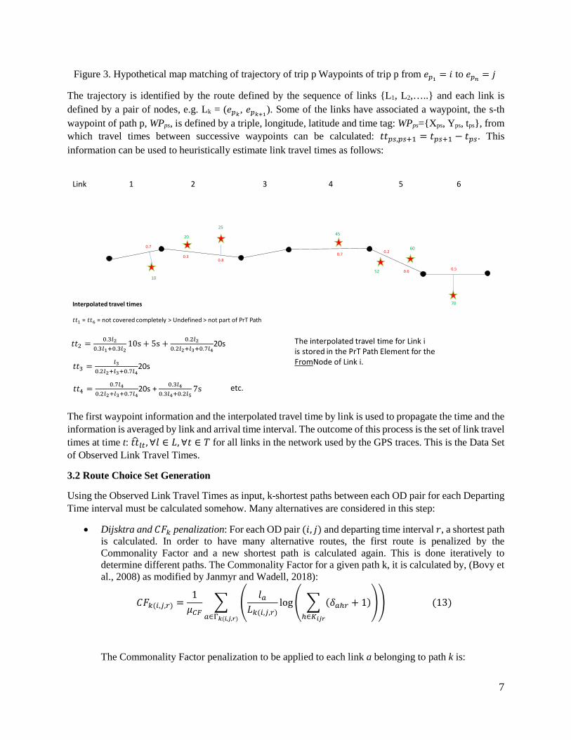
Figure 3. Hypothetical map matching of trajectory of trip p Waypoints of trip p from 𝐴𝐴𝑝𝑝1 = 𝑚𝑚 to 𝐴𝐴𝑝𝑝𝑛𝑛 = 𝑗𝑗

The trajectory is identified by the route defined by the sequence of links {L1, L2,…..} and each link is defined by a pair of nodes, e.g. Lk = (𝐴𝐴𝑝𝑝𝑘𝑘, 𝐴𝐴𝑝𝑝𝑘𝑘+1). Some of the links have associated a waypoint, the s-th waypoint of path p, WPps, is defined by a triple, longitude, latitude and time tag: WPps={Xps, Yps, tps}, from which travel times between successive waypoints can be calculated: 𝐴𝐴𝐴𝐴𝑝𝑝𝑝𝑝,𝑝𝑝𝑝𝑝+1 = 𝐴𝐴𝑝𝑝𝑝𝑝+1 − 𝐴𝐴𝑝𝑝𝑝𝑝. This information can be used to heuristically estimate link travel times as follows:

The first waypoint information and the interpolated travel time by link is used to propagate the time and the information is averaged by link and arrival time interval. The outcome of this process is the set of link travel times at time t: 𝐴𝐴𝐴𝐴�𝑙𝑙𝑙𝑙,∀𝑙𝑙 ∈ 𝐿𝐿,∀𝐴𝐴 ∈ 𝑇𝑇 for all links in the network used by the GPS traces. This is the Data Set of Observed Link Travel Times.

3.2 Route Choice Set Generation

Using the Observed Link Travel Times as input, k-shortest paths between each OD pair for each Departing Time interval must be calculated somehow. Many alternatives are considered in this step:

• Dijsktra and 𝐶𝐶𝐹𝐹𝑘𝑘 penalization: For each OD pair (𝑚𝑚, 𝑗𝑗) and departing time interval 𝑟𝑟, a shortest path is calculated. In order to have many alternative routes, the first route is penalized by the Commonality Factor and a new shortest path is calculated again. This is done iteratively to determine different paths. The Commonality Factor for a given path k, it is calculated by, (Bovy et al., 2008) as modified by Janmyr and Wadell, 2018):

𝐶𝐶𝐹𝐹𝑘𝑘(𝑖𝑖,𝑖𝑖,𝑖𝑖) =1𝜇𝜇𝐶𝐶𝐶𝐶

� �𝑙𝑙𝑎𝑎

𝐿𝐿𝑘𝑘(𝑖𝑖,𝑖𝑖,𝑖𝑖)log� � (𝛿𝛿𝑎𝑎ℎ𝑖𝑖 + 1)

ℎ∈𝐾𝐾𝑖𝑖𝑖𝑖𝑖𝑖

�� (13)𝑎𝑎∈Γ𝑘𝑘(𝑖𝑖,𝑖𝑖,𝑖𝑖)

The Commonality Factor penalization to be applied to each link a belonging to path k is:

Link 1 2 3 4 5 6

0.7

0.30.8

0.7 0.2

0.6 0.5

10

20

2545

52

60

70Interpolated travel times

𝐴𝐴𝐴𝐴1 = 𝐴𝐴𝐴𝐴6 = not covered completely > Undefined > not part of PrT Path

𝐴𝐴𝐴𝐴2 = 0.3𝑙𝑙20.3𝑙𝑙1+0.3𝑙𝑙2

10s + 5s + 0.2𝑙𝑙20.2𝑙𝑙2+𝑙𝑙3+0.7𝑙𝑙4

20s

𝐴𝐴𝐴𝐴3 = 𝑙𝑙30.2𝑙𝑙2+𝑙𝑙3+0.7𝑙𝑙4

20s

The interpolated travel time for Link iis stored in the PrT Path Element for theFromNode of Link i.

𝐴𝐴𝐴𝐴4 = 0.7𝑙𝑙40.2𝑙𝑙2+𝑙𝑙3+0.7𝑙𝑙4

20s + 0.3𝑙𝑙40.3𝑙𝑙4+0.2𝑙𝑙5

7s etc.

8

𝐶𝐶𝐹𝐹𝑎𝑎(𝑘𝑘(𝑖𝑖,𝑖𝑖,𝑖𝑖)) =1𝜇𝜇𝐶𝐶𝐶𝐶

�𝑙𝑙𝑎𝑎

𝐿𝐿𝑘𝑘(𝑖𝑖,𝑖𝑖,𝑖𝑖)log� � (𝛿𝛿𝑎𝑎ℎ𝑖𝑖 + 1)

ℎ∈𝐾𝐾𝑖𝑖𝑖𝑖𝑖𝑖

��

where 𝐾𝐾𝑖𝑖𝑖𝑖𝑖𝑖 is the calculated set of paths for (𝑚𝑚, 𝑗𝑗)-OD pair at 𝑟𝑟 departing time interval, 𝑙𝑙𝑎𝑎 is the length of the link and 𝐿𝐿𝑘𝑘(𝑖𝑖,𝑖𝑖,𝑖𝑖) is the total length of the shortest path for set 𝐾𝐾𝑖𝑖𝑖𝑖𝑖𝑖. Γ𝑘𝑘(𝑖𝑖,𝑖𝑖,𝑖𝑖) is the sequence of links for path 𝑘𝑘 and 𝛿𝛿𝑎𝑎ℎ𝑖𝑖 ∈ {0,1} indicates whether link a does belong to path h included in the calculated path set 𝐾𝐾𝑖𝑖𝑖𝑖𝑖𝑖 or not. This alternative is computationally expensive because it requires |𝑰𝑰| × |𝑱𝑱| × |𝑻𝑻| × 𝒌𝒌 shortest path algorithm evaluations.

• S-HEAP algorithm: In order to reduce the computational effort. The algorithm can be changed to a Shortest Path Tree algorithm for each origin, using (Gallo and Pallotino, 1988) algorithm.

o Similarly, to the first option, an iterative procedure must be used to compute k-shortest paths, using the same penalization.

o In this case, the computational effort is reduced to |𝑰𝑰| × |𝑻𝑻| × 𝒌𝒌 evaluations of the

algorithm. However, each individual step is a bit more expensive in time.

• Assignment: This option is to use an auxiliary Dynamic Assignment in order to obtain the different paths for each OD pair and each time interval. The role of this auxiliary Dynamic Assignment in this case is not that of providing an t assignment matrix, as in the analytical formulation, it is only an auxiliary tool to generate the paths that are used at each time interval. This option is weak in the sense that it will be contradictory with the name “Assignment Free DODE”, but is an acceptable option to produce a first “Proof of Concept” of the algorithm, due to its easy implementation.

• k-Time Dependent Shortest Paths: This was the main option because it is the most accurate since it considers the proper calculation of the k time dependent shortest paths (TDSP). The proposed algorithm to find the k-TDSP is (Chabini, 1997). This option is the most complex, so it requires more implementation effort and also computational time. However, from our previous experience, at the moment the increase in quality does not justify the implementation effort for the Proof of Concept purpose.

3.3. Calculation of 𝑪𝑪𝑭𝑭𝒌𝒌 and 𝑷𝑷𝒌𝒌

At this step, the input is a set of calculated paths, 𝐾𝐾𝑖𝑖𝑖𝑖𝑖𝑖, for each origin 𝑚𝑚, destination 𝑗𝑗 and departing time 𝑟𝑟. These paths are noted by 𝑘𝑘(𝑚𝑚, 𝑗𝑗, 𝑟𝑟) ∈ 𝐾𝐾𝑖𝑖𝑖𝑖𝑖𝑖, to show explicitely the dependence to (𝑚𝑚, 𝑗𝑗, 𝑟𝑟). For a certain path 𝑘𝑘(𝑚𝑚, 𝑗𝑗, 𝑟𝑟), the sequence of links is the set Γ𝑘𝑘(𝑖𝑖,𝑖𝑖,𝑖𝑖) = {𝐴𝐴1, … , 𝐴𝐴𝑚𝑚𝑘𝑘 }.

The path choice for each path on the set 𝐾𝐾𝑖𝑖𝑖𝑖𝑖𝑖 is calculated as a discrete choice model that uses the commonality factor, 𝐶𝐶𝐹𝐹𝑘𝑘, as a penalization factor on travel times, (Nassir et al., 2014). That is:

𝐶𝐶𝐹𝐹𝑘𝑘(𝑖𝑖,𝑖𝑖,𝑖𝑖) =1𝜇𝜇𝐶𝐶𝐶𝐶

� �𝑙𝑙𝑎𝑎

𝐿𝐿𝑘𝑘(𝑖𝑖,𝑖𝑖,𝑖𝑖)log� � (𝛿𝛿𝑎𝑎ℎ𝑖𝑖 + 1)

ℎ∈𝐾𝐾𝑖𝑖𝑖𝑖𝑖𝑖

��𝑎𝑎∈Γ𝑘𝑘(𝑖𝑖,𝑖𝑖,𝑖𝑖)

9

𝑊𝑊𝑘𝑘(𝑖𝑖,𝑖𝑖,𝑖𝑖) =exp�𝜇𝜇𝑝𝑝�−𝐴𝐴𝐴𝐴�𝑘𝑘(𝑖𝑖,𝑖𝑖,𝑖𝑖) − 𝐶𝐶𝐹𝐹𝑘𝑘(𝑖𝑖,𝑖𝑖,𝑖𝑖)��

∑ exp�𝜇𝜇𝑝𝑝�−𝐴𝐴𝐴𝐴�ℎ(𝑖𝑖,𝑖𝑖,𝑖𝑖) − 𝐶𝐶𝐹𝐹ℎ(𝑖𝑖,𝑖𝑖,𝑖𝑖)��ℎ∈𝐾𝐾𝑖𝑖𝑖𝑖𝑖𝑖 (14)

These calculations permit to obtain the flow distribution for each path, based on observed path travel times. These observed path travel times are the summation of the observed link travel times, considering the arrival time, t(k), at each link a, included in the path k:

𝐴𝐴𝐴𝐴�𝑘𝑘(𝑖𝑖,𝑖𝑖,𝑖𝑖) = � 𝐴𝐴𝐴𝐴�𝑎𝑎𝑙𝑙(𝑘𝑘)𝑎𝑎∈Γ𝑘𝑘(𝑖𝑖,𝑖𝑖,𝑖𝑖)

(15)

3.4. Calculation of the Time Dependent Assignment Matrix

Once 𝑷𝑷𝒌𝒌 = [𝑊𝑊𝑘𝑘(𝑖𝑖,𝑖𝑖,𝑖𝑖)] is calculated from the k-shortest paths calculated after the travel times estimated from the GPS data for all OD pairs, the empirical assignment matrix �𝑎𝑎�𝑖𝑖𝑖𝑖𝑖𝑖𝑙𝑙𝑙𝑙 � can be calculated:

𝑎𝑎�𝑖𝑖𝑖𝑖𝑖𝑖𝑙𝑙𝑙𝑙 = � 𝛿𝛿𝑘𝑘(𝑖𝑖,𝑖𝑖,𝑖𝑖)𝑙𝑙𝑙𝑙 𝑊𝑊𝑘𝑘(𝑖𝑖,𝑖𝑖,𝑖𝑖)

𝑘𝑘∈𝐾𝐾𝑖𝑖𝑖𝑖𝑖𝑖

∀𝑚𝑚, 𝑗𝑗, 𝑟𝑟, 𝑙𝑙, 𝐴𝐴 (16)

where 𝛿𝛿𝑘𝑘(𝑖𝑖,𝑖𝑖,𝑖𝑖)𝑙𝑙𝑙𝑙 is the empirical incidence indicator:

𝛿𝛿𝑘𝑘(𝑖𝑖,𝑖𝑖,𝑖𝑖)𝑙𝑙𝑙𝑙 = �1 if path 𝑘𝑘(𝑚𝑚, 𝑗𝑗, 𝑟𝑟) uses link 𝑙𝑙 at time 𝐴𝐴

0 otherwise

3.5 An Assignment Free DODME Approach The introduction in Section 1 to the analytical approaches to DODME problem, and the discussion of their extensions in Section 2, shows that all are based on the availability of the Assignment Matrix A. And the main role of the Dynamic Traffic Assignment at the lower level of (1) is just to provide this estimate at each time interval. However, the availability of the GPS tracking data, and the proposed methodological analysis, enables us to assume that the paths 𝐾𝐾�𝑖𝑖𝑖𝑖𝑖𝑖 calculated in 3.2, and the path choices (14) in 3.3 can be interpreted in terms of an empirical dynamic assignment. Then the empirical assignment matrix (16) plays the same role as the analytical assignment matrix estimated in Section 2 from the Dynamic Traffic Assignment. Considering that the dynamic formulation of (1) model decomposes it into time intervals to emulate the flow propagation across the network, assuming that at each iteration of the optimization procedure the relationships between the estimated flows and the adjusted matrix can be set up in terms of a time dependent assignment matrix (2). Then stopping the Taylor expansion in the first order terms, as in (5), Toledo and Koleckhina (2013), Frederix et al (2013), Ros-Roca et al. (2019), and replacing the analytical by the empirical assignment matrix (16) the relationship between the link flows and the OD matrix can be restated as:

𝑦𝑦𝑙𝑙𝑙𝑙 = ���𝑎𝑎𝑖𝑖𝑖𝑖𝑖𝑖𝑙𝑙𝑙𝑙 𝑥𝑥𝑖𝑖𝑖𝑖𝑖𝑖

𝑙𝑙

𝑖𝑖=1𝑖𝑖∈𝐽𝐽𝑖𝑖∈𝐼𝐼

(17)

10

where 𝑦𝑦𝑙𝑙𝑙𝑙 is the estimated flow in link l at time period t, 𝑥𝑥𝑖𝑖𝑖𝑖𝑖𝑖 is the flow departing origin 𝑚𝑚 ∈ 𝐼𝐼 =

{𝐴𝐴𝐴𝐴𝐴𝐴 𝑓𝑓𝑓𝑓 𝑓𝑓𝑟𝑟𝑚𝑚𝐴𝐴𝑚𝑚𝑚𝑚𝐴𝐴}, with destination 𝑗𝑗 ∈ 𝐽𝐽 = {𝐴𝐴𝐴𝐴𝐴𝐴 𝑓𝑓𝑓𝑓 𝑑𝑑𝐴𝐴𝐴𝐴𝐴𝐴𝑚𝑚𝑚𝑚𝑎𝑎𝐴𝐴𝑚𝑚𝑓𝑓𝑚𝑚𝐴𝐴}, at time interval r, and 𝑎𝑎𝑖𝑖𝑖𝑖𝑖𝑖𝑙𝑙𝑙𝑙 , the empirical

assignment matrix, is the fraction of trips from origin 𝑚𝑚 ∈ 𝐼𝐼 with destination 𝑗𝑗 ∈ 𝐽𝐽, departing from i at time r, that reach link l at time t. Then, assuming that traffic counts measured by real detectors placed onto the network are available. They are measured for each time interval and denoted by: 𝑦𝑦�𝑙𝑙𝑙𝑙, where 𝑙𝑙 ⊆ 𝐿𝐿� is the link with the detector of the network and 𝐴𝐴 the time interval when it is measured. The research question addressed in this research report can be formulated in the following terms: if the data collected from a sample of GPS tracked vehicles provide us with a discretized time estimate of the target OD matrix 𝑿𝑿� = �𝑥𝑥�𝑖𝑖𝑖𝑖𝑖𝑖�, and a suitable processing, Janmyr and Wadell (2018), Krishnakumari et al. (2019), Nassir (2014), provides a sound empirical estimate of 𝑎𝑎𝑖𝑖𝑖𝑖𝑖𝑖

𝑙𝑙𝑙𝑙 , then the expansion of the sampled target matrix to estimate the OD matrix can be done in terms of the scaling factors per origins, 𝛼𝛼𝑖𝑖, 𝑚𝑚 ∈ 𝐼𝐼, and per destinations 𝛽𝛽𝑖𝑖, 𝑗𝑗 ∈ 𝐽𝐽, such that:

𝑥𝑥𝑖𝑖𝑖𝑖𝑖𝑖 = 𝛼𝛼𝑖𝑖𝛽𝛽𝑖𝑖𝑥𝑥�𝑖𝑖𝑖𝑖𝑖𝑖 ,∀𝑚𝑚 ∈ 𝐼𝐼,∀𝑗𝑗 ∈ 𝐽𝐽,∀𝑟𝑟 ∈ 𝑇𝑇 (18) If 𝑦𝑦�𝑙𝑙𝑙𝑙 , 𝑙𝑙 ∈ 𝐿𝐿� ⊂ 𝐿𝐿, 𝐴𝐴 ∈ 𝑇𝑇 are the link flows measured at the counting stations, in a subset 𝐿𝐿� ⊂ 𝐿𝐿 of the network links, the Dynamic Data-Driven OD Matrix Estimation problem can be formulated as the following optimization problem of finding the values of the scaling factors 𝛼𝛼𝑖𝑖, 𝑚𝑚 ∈ 𝐼𝐼 and 𝛽𝛽𝑖𝑖, 𝑗𝑗 ∈ 𝐽𝐽, without the need of conducting the traffic assignment at the lower level of (1), exploiting the empirical assignment matrix 𝑎𝑎𝑖𝑖𝑖𝑖𝑖𝑖

𝑙𝑙𝑙𝑙 . However, if an historical OD is available from other sources, then a seed matrix 𝑥𝑥𝑖𝑖𝑖𝑖𝑖𝑖0 can be generated combining that historical OD matrix 𝑥𝑥𝑖𝑖𝑖𝑖𝑖𝑖𝐻𝐻 and the observed OD matrix 𝑥𝑥�𝑖𝑖𝑖𝑖𝑖𝑖 obtained from GPS tracked trips, and it is denoted as 𝑿𝑿𝟎𝟎 = �𝑥𝑥𝑖𝑖𝑖𝑖𝑖𝑖0 �. From (17) and (18) the proposed new formulation of the DODME problem is:

min𝛼𝛼𝑖𝑖,𝛽𝛽𝑖𝑖

���𝑦𝑦�𝑙𝑙𝑙𝑙 − �𝛼𝛼𝑖𝑖𝛽𝛽𝑖𝑖𝑎𝑎𝑖𝑖𝑖𝑖𝑖𝑖𝑙𝑙𝑙𝑙 𝑥𝑥𝑖𝑖𝑖𝑖𝑖𝑖0

𝑖𝑖,𝑖𝑖,𝑖𝑖

�

2

𝑙𝑙,𝑙𝑙

� (19)

𝐴𝐴. 𝐴𝐴. 𝛼𝛼𝑖𝑖 ,𝛽𝛽𝑖𝑖 ≥ 0

The variables of the problem are multiplicative scaling factors for each origin, 𝛼𝛼𝑖𝑖, and destination, 𝛽𝛽𝑖𝑖. They are inspired on gravity models where bi-dimensional constraints for rows and columns are set. The minimization problem is solved iteratively with the L-BFGS-B method appropriated for constrained non-linear problems using the version available in python package scipy.optimize.

The conceptual computational scheme of the proposed Assignment Free DODME approach, powered by the ICT applications capturing GPS data trajectories is depicted in Figure 4.

11

Figure 4. A Data Driven Assignment Free DODME

4. A computational proof of concept of the Assignment Free data Driven DODME

A first test with the Torino CDB subnetwork, Figure 5, has been conducted in order to check the functional feasibility of the algorithmic chain, Figure 4, of the new approach.

12

Figure 5: Torino CBD Subnetwork

A summary of the model and the real inputs is shown in the Table 2:

Table 2: Torino’s CBD Experiment characteristics

TIME PERIODS 4 ZONES 268 DETECTORS 582 OD PAIRS X TIME 287k INRIX WAYPOINTS 2.9M INRIX TRIPS 166k OBS OD > 0 32k (12%) HIST OD > 0 120k (42%)

4.1. GPS Data: Building the Seed OD matrix [yellow circle Method in Figure 4]

6 months of GPS data coming from INRIX for all Piemonte region are available. These are 220M waypoints for 5.9M trips. There is no further information regarding the type of vehicle (fleet/private) and it points that there was no distinction between them. Consequently, the only filtering that can be done relies on zoning and weekday selection.

After the pre-processing and filtering steps, the final dataset of waypoints (GPX file) contains 2.9M of waypoints for 166k trips (reduction to the 1.31% of the raw data). The observed OD matrix, 𝑥𝑥�𝑖𝑖𝑖𝑖𝑖𝑖, has 32k positive values, which is the 12% of the matrix.

The GPS data have to be preprocessed in order to filter the useful data for the method proposed in this research paper. In a first step, only weekdays trips (Tuesday, Wednesday and Thursday) in the considered time interval have been selected.

13

After that, using a SHP file with the information of the Transportation Zoning System (TAZ) of the model, an Origin and a Destination Zone has been assigned to each trip. Those trips that begin and/or end out of the study area, are cut and considered to be started/ended on the first/last zone of the network where they are observed. There are two outputs of this procedure: GPX file: This GPX file is generated with the filtered and processed trips. They are coded in a GPX

file to be inserted in VISUM GPX import tool. Observed OD matrix: The filtered and processed trips are counted by Origin, Destination and

Departing Time to be translated to an observed OD matrix, 𝑥𝑥�𝑖𝑖𝑖𝑖𝑖𝑖. Remark: The experience gained preprocessing the INRIX data shows they could be two questionable issues:

a) The mix of data from commercial fleets and private vehicles that must be properly filtered.

b) The bias that can be induced by the data collection process splitting long trips in shorter trips due to privacy issues, in which case a significant fraction of origins and destinations do not correspond to the underlying mobility pattern.

These drawbacks are independent on the size of the sample, since they are inherent to the data collection procedure, designed for other purposes than the OD matrix estimation. This is one of the reasons to consider this computational testing only as a proof of concept since we cannot ensure the quality of the inputs, and therefore assess the quality of the outputs.

After the Map Matching into VISUM, the total number of PrTPaths is 130k, which means the 78% of the sample. This loss is acceptable due to the short trips.

The observed link travel times per time interval, 𝐴𝐴𝐴𝐴�𝑙𝑙𝑙𝑙, computed by averaging the PrTPaths’ Interpolated travel times at link level after propagating the time, covers the major part of network, resulting a connected network, Figure 6. Furthermore, the number of observations per link and time interval is right-skewed distributed as shown:

min Q1 Median Mean Q3 max 1 7 24 50 69 658

We observed that the more observations a link has, the lower the standard deviation of its travel times is, which is consistent.

14

Figure 6: Links with observed link travel time.

Regarding the possibility of not finding shortest paths because there could be not connected zones, the preliminary test with a set of OD pairs showed that the connectivity is not a problem, since up to the 93% of the times, a shortest path is found.

Some tests using Shortest Path Visum show the goodness of these observed travel times. Figure 7 shows an example of the shortest path calculation between two nodes calculated using the free-flow travel time (left) and the observed travel time (right).

Figure 7: Comparison of shortest paths between t0 and observed travel time.

15

However, the use of the shortest path tool of Visum is not feasible because of its computational time. It takes 0.6 seconds for each path, which for each OD pair and time interval is approximately: 268·268·4·0.6sec = 143,468sec = 40h = 1day16h. Other alternatives as those listed before must be considered.

4.2. Dynamic Stochastic Assignment as Route Choice Set

For the proof of concept, the Route Choice Set Generation has been substituted by the Dynamic Stochastic Assignment (10 iterations) available in Visum as a shortcut to define the calculated paths for each OD pair at each time interval. For these paths, commonality factors and path proportions, 𝐶𝐶𝐹𝐹𝑘𝑘 and 𝑊𝑊𝑘𝑘 , are calculated using the observed link travel times coming from the processing of the GPS data.

4.3. Calculation of 𝑪𝑪𝑭𝑭𝒌𝒌 , 𝑷𝑷𝒌𝒌 and 𝒂𝒂�𝒏𝒏𝒓𝒓𝒍𝒍𝒓𝒓 and Optimization

The calculation of 𝐶𝐶𝐹𝐹𝑘𝑘, 𝑊𝑊𝑘𝑘 and 𝑎𝑎𝑖𝑖𝑖𝑖𝑖𝑖𝑙𝑙𝑙𝑙 has been conducted applying (14), (15) and (16). The objective function

(19) shows a nice and fast decrease and convergence, see Figure 8.

Figure 8: Descent of the Objective Function

The seed OD matrix, 𝑥𝑥𝑖𝑖𝑖𝑖𝑖𝑖0 , is in this case the Historical OD matrix for Torino, i.e., 𝑥𝑥𝑖𝑖𝑖𝑖𝑖𝑖0 = 𝑥𝑥𝑖𝑖𝑖𝑖𝑖𝑖𝐻𝐻 . An analysis of the evolution of traffic counts is shown in Figure 9:

16

Figure 9: Traffic Flow counts before and after the optimization procedure.

The initial 𝑅𝑅2 is 0.33 and the final 𝑅𝑅2 is 0.66.

4.4. Summary of Computational Times

Preprocess and filtering of GPS Data -> 50 minutes Import GPX tool -> 4h 21minutes Link Travel Times Computation -> 6minutes Dynamic Stochastic Assignment -> 13minutes Calculation of 𝐶𝐶𝐹𝐹𝑘𝑘, 𝑊𝑊𝑘𝑘 and 𝑎𝑎�𝑖𝑖𝑖𝑖𝑖𝑖𝑙𝑙𝑙𝑙 -> 1minute Optimization -> 10minutes/iteration

5. Alternative Assigment Free DODME proposal

- Assuming that a time sliced historical OD matrix 𝑿𝑿𝑯𝑯 is available - The expansion of the sample 𝑥𝑥𝑖𝑖𝑖𝑖𝑖𝑖0 is bounded from below by 𝑙𝑙𝑙𝑙𝑖𝑖𝑖𝑖𝑖𝑖 and from above by 𝑢𝑢𝑙𝑙𝑖𝑖𝑖𝑖𝑖𝑖, accounting

explicitly for the socioeconomic characteristics of the TAZ - Weights 𝑤𝑤1 and 𝑤𝑤2 on the distance functions

min𝛼𝛼𝑖𝑖,𝛽𝛽𝑖𝑖

�𝑤𝑤1 �����𝑥𝑥𝑖𝑖𝑖𝑖𝑖𝑖𝐻𝐻 − 𝛼𝛼𝑖𝑖𝛽𝛽𝑖𝑖𝑥𝑥𝑖𝑖𝑖𝑖𝑖𝑖0 �2

𝑖𝑖∈𝑇𝑇𝑖𝑖∈𝐽𝐽𝑖𝑖∈𝐼𝐼

� + 𝑤𝑤2���𝑦𝑦�𝑙𝑙𝑙𝑙 −���𝑎𝑎�𝑖𝑖𝑖𝑖𝑖𝑖𝑙𝑙𝑙𝑙 𝛼𝛼𝑖𝑖𝛽𝛽𝑖𝑖𝑥𝑥𝑖𝑖𝑖𝑖𝑖𝑖0𝑙𝑙

𝑖𝑖=1𝑖𝑖∈𝐽𝐽𝑖𝑖∈𝐼𝐼

�

2

𝑙𝑙𝑙𝑙𝐿𝐿�𝑙𝑙∈𝑇𝑇

� (20)

𝑙𝑙𝑙𝑙𝑖𝑖𝑖𝑖𝑖𝑖 ≤ 𝛼𝛼𝑖𝑖𝛽𝛽𝑖𝑖𝑥𝑥𝑖𝑖𝑖𝑖𝑖𝑖0 ≤ 𝑢𝑢𝑙𝑙𝑖𝑖𝑖𝑖𝑖𝑖,∀𝑚𝑚 ∈ 𝐼𝐼,∀𝑗𝑗 ∈ 𝐽𝐽,∀𝑟𝑟 ∈ 𝑇𝑇

𝛼𝛼𝑖𝑖 ≥ 0,∀𝑚𝑚 ∈ 𝐼𝐼

𝛽𝛽𝑖𝑖 ≥ 0,∀𝑗𝑗 ∈ 𝐽𝐽

5.1 Variant 1

However, while enabling to capture the underlying physical characteristics of the underlying transport system, this formulation has the drawback of the high number of non-linear constraints:

𝑙𝑙𝑙𝑙𝑖𝑖𝑖𝑖𝑖𝑖 ≤ 𝛼𝛼𝑖𝑖𝛽𝛽𝑖𝑖𝑥𝑥𝑖𝑖𝑖𝑖𝑖𝑖0 ≤ 𝑢𝑢𝑙𝑙𝑖𝑖𝑖𝑖𝑖𝑖,∀𝑚𝑚 ∈ 𝐼𝐼,∀𝑗𝑗 ∈ 𝐽𝐽,∀𝑟𝑟 ∈ 𝑇𝑇

|𝐼𝐼| × |𝐽𝐽| × |𝑇𝑇|. Summing for i and j the lower and upper bounds respectively, one can obtain aggregated bounds that instead bounding each cell (𝑚𝑚, 𝑗𝑗) bound, respectively, the generation and attraction characteristics of each TAZ:

𝐿𝐿𝐿𝐿𝑖𝑖𝑖𝑖 = �𝑙𝑙𝑙𝑙𝑖𝑖𝑖𝑖𝑖𝑖𝑖𝑖∈𝐽𝐽

𝑎𝑎𝑚𝑚𝑑𝑑 𝑈𝑈𝐿𝐿𝑖𝑖𝑖𝑖 = �𝑢𝑢𝑙𝑙𝑖𝑖𝑖𝑖𝑖𝑖𝑖𝑖∈𝐽𝐽

∀𝑚𝑚 ∈ 𝐼𝐼,∀𝑟𝑟 ∈ 𝑇𝑇

𝐿𝐿𝐿𝐿𝑖𝑖𝑖𝑖 = �𝑙𝑙𝑙𝑙𝑖𝑖𝑖𝑖𝑖𝑖𝑖𝑖∈𝐼𝐼

𝑎𝑎𝑚𝑚𝑑𝑑 𝑈𝑈𝑊𝑊𝑖𝑖𝑖𝑖 = �𝑢𝑢𝑙𝑙𝑖𝑖𝑖𝑖𝑖𝑖𝑖𝑖∈𝐼𝐼

∀𝑗𝑗 ∈ 𝐽𝐽,∀𝑟𝑟 ∈ 𝑇𝑇

Then the set of bounding constraints can be reformulated as:

17

𝐿𝐿𝐿𝐿𝑖𝑖𝑖𝑖 ≤ 𝛼𝛼𝑖𝑖�𝛽𝛽𝑖𝑖𝑥𝑥𝑖𝑖𝑖𝑖𝑖𝑖0

𝑖𝑖∈𝐽𝐽

≤ 𝑈𝑈𝐿𝐿𝑖𝑖𝑖𝑖 ∀𝑚𝑚 ∈ 𝐼𝐼,∀𝑟𝑟 ∈ 𝑇𝑇 (21)

𝐿𝐿𝐿𝐿𝑖𝑖𝑖𝑖 ≤ 𝛽𝛽𝑖𝑖�𝛼𝛼𝑖𝑖𝑖𝑖𝑙𝑙𝐼𝐼

𝑥𝑥𝑖𝑖𝑖𝑖𝑖𝑖0 ≤ 𝑈𝑈𝐿𝐿𝑖𝑖𝑖𝑖 ∀𝑗𝑗 ∈ 𝐽𝐽,∀𝑟𝑟 ∈ 𝑇𝑇 (22)

That is (|𝐼𝐼| + |𝐽𝐽|) × |𝑇𝑇| non-linear constraints.

5.2 Variant 2

However, from a computational perspective while reducing significantly the size of the constraint set, the sets of constraints (21) and (22) still have a major computational disadvantage since they are nonlinear constraints. A suitable approximation, replacing them by linear ones, could improve the computational performance while holding the main physical characteristics of the underlying transport problem.

The formulation (20) assumes that the entry cell (i,j) of the estimated OD matrix for time period r, 𝑥𝑥𝑖𝑖𝑖𝑖𝑖𝑖 is given by:

𝑥𝑥𝑖𝑖𝑖𝑖𝑖𝑖 = 𝛼𝛼𝑖𝑖𝛽𝛽𝑖𝑖𝑥𝑥𝑖𝑖𝑖𝑖𝑖𝑖0

Then the trip generation of origin i for time period r is given by:

𝑂𝑂𝑖𝑖𝑖𝑖 = �𝑥𝑥𝑖𝑖𝑖𝑖𝑖𝑖𝑖𝑖∈𝐽𝐽

= �𝛼𝛼𝑖𝑖𝛽𝛽𝑖𝑖𝑥𝑥𝑖𝑖𝑖𝑖𝑖𝑖0

𝑖𝑖∈𝐽𝐽

= 𝛼𝛼𝑖𝑖�𝛽𝛽𝑖𝑖𝑖𝑖∈𝐽𝐽

𝑥𝑥𝑖𝑖𝑖𝑖𝑖𝑖0 →𝑂𝑂𝑖𝑖𝑖𝑖𝛼𝛼𝑖𝑖

= �𝛽𝛽𝑖𝑖𝑖𝑖∈𝐽𝐽

𝑥𝑥𝑖𝑖𝑖𝑖𝑖𝑖0 (23)

Let’s assume that:

- 𝑂𝑂�𝑖𝑖𝑖𝑖 is an estimate of 𝑂𝑂𝑖𝑖𝑖𝑖, for instance from a suitable historical OD matrix 𝑿𝑿𝑯𝑯. Remark, this could be a good chance to include alternative OD sources, as for example those from KINEO’s (or similar matrices from Smartphones) in this “fusion” procedure.

- If upper and lower bounds for 𝛼𝛼𝑖𝑖, 𝛼𝛼𝑖𝑖𝑙𝑙, and 𝛼𝛼𝑖𝑖𝑢𝑢, respectively, can be estimated such that 𝛼𝛼𝑖𝑖 ∈ �𝛼𝛼𝑖𝑖𝑙𝑙 ,𝛼𝛼𝑖𝑖𝑢𝑢�

Then:

𝑈𝑈𝐿𝐿� 𝑖𝑖𝑖𝑖 =𝑂𝑂�𝑖𝑖𝑖𝑖𝛼𝛼𝑖𝑖𝑙𝑙

𝑎𝑎𝑚𝑚𝑑𝑑 𝐿𝐿𝐿𝐿�𝑖𝑖𝑖𝑖 =𝑂𝑂�𝑖𝑖𝑖𝑖𝛼𝛼𝑖𝑖𝑢𝑢

Would respectively be upper and lower bound estimates of (23), and then, constraints (21) could be approximated by:

𝐿𝐿𝐿𝐿�𝑖𝑖𝑖𝑖 ≤�𝛽𝛽𝑖𝑖𝑖𝑖∈𝐽𝐽

𝑥𝑥𝑖𝑖𝑖𝑖𝑖𝑖0 ≤ 𝑈𝑈𝐿𝐿�𝑖𝑖𝑖𝑖, ∀𝑚𝑚 ∈ 𝐼𝐼,∀𝑟𝑟 ∈ 𝑇𝑇 (24)

Similarly:

𝐷𝐷𝑖𝑖𝑖𝑖 = �𝑥𝑥𝑖𝑖𝑖𝑖𝑖𝑖𝑖𝑖∈𝐼𝐼

= �𝛼𝛼𝑖𝑖𝛽𝛽𝑖𝑖𝑥𝑥𝑖𝑖𝑖𝑖𝑖𝑖0

𝑖𝑖∈𝐼𝐼

= 𝛽𝛽𝑖𝑖�𝛼𝛼𝑖𝑖𝑖𝑖∈𝐼𝐼

𝑥𝑥𝑖𝑖𝑖𝑖𝑖𝑖0 →𝐷𝐷𝑖𝑖𝑖𝑖𝛽𝛽𝑖𝑖

= �𝛼𝛼𝑖𝑖𝑖𝑖∈𝐼𝐼

𝑥𝑥𝑖𝑖𝑖𝑖𝑖𝑖0 (25)

Then, if:

- 𝐷𝐷�𝑖𝑖𝑖𝑖 is an estimate of 𝐷𝐷𝑖𝑖𝑖𝑖, for instance from a suitable historical OD matrix 𝑿𝑿𝑯𝑯.

18

- And upper and lower bounds for 𝛽𝛽𝑖𝑖, 𝛽𝛽𝑖𝑖𝑙𝑙, and 𝛽𝛽𝑖𝑖𝑢𝑢, respectively, can be estimated such that 𝛽𝛽𝑖𝑖 ∈�𝛽𝛽𝑖𝑖𝑙𝑙,𝛽𝛽𝑖𝑖𝑢𝑢�

𝑈𝑈𝐿𝐿�𝑖𝑖𝑖𝑖 =𝐷𝐷�𝑖𝑖𝑖𝑖𝛽𝛽𝑖𝑖𝑙𝑙

𝑎𝑎𝑚𝑚𝑑𝑑 𝐿𝐿𝐿𝐿�𝑖𝑖𝑖𝑖 =𝐷𝐷�𝑖𝑖𝑖𝑖𝛽𝛽𝑖𝑖𝑢𝑢

Would, respectively, be upper and lower bound estimates of (6), and then, constraints (3) could be approximated by:

𝐿𝐿𝐿𝐿�𝑖𝑖𝑖𝑖 ≤�𝛼𝛼𝑖𝑖𝑖𝑖∈𝐼𝐼

𝑥𝑥𝑖𝑖𝑖𝑖𝑖𝑖0 ≤ 𝑈𝑈𝐿𝐿�𝑖𝑖𝑖𝑖, ∀𝑗𝑗 ∈ 𝐽𝐽,∀𝑟𝑟 ∈ 𝑇𝑇 (26)

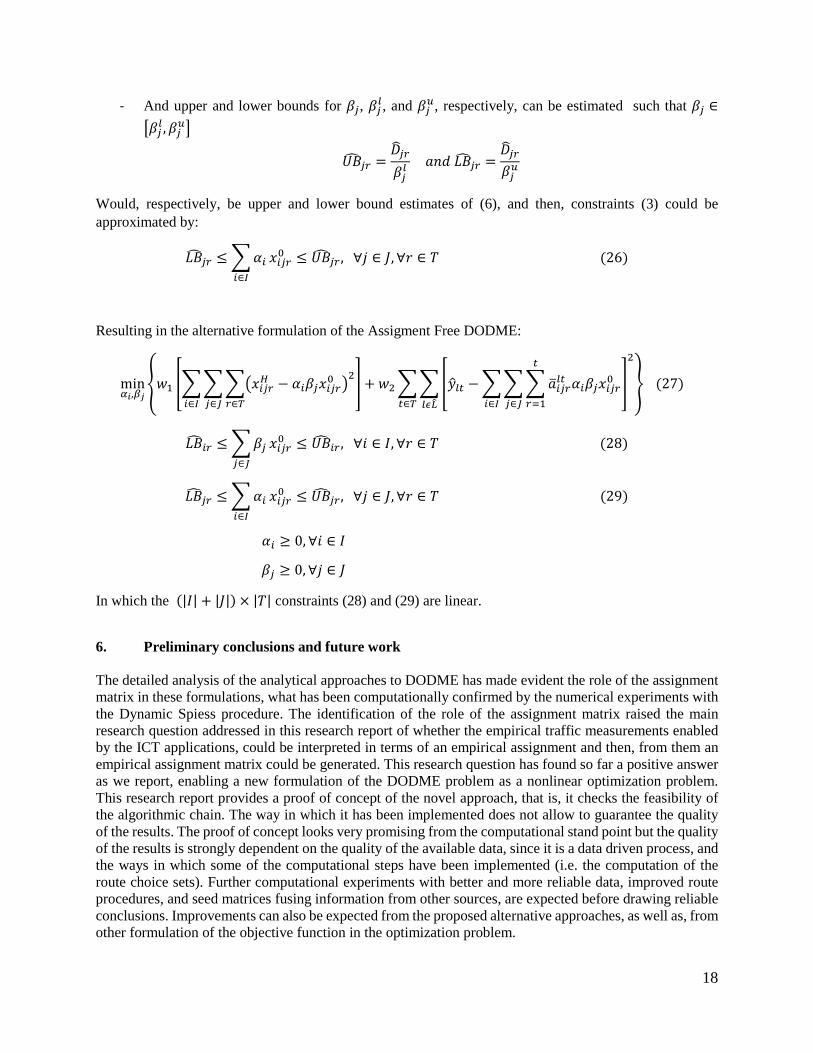
Resulting in the alternative formulation of the Assigment Free DODME:

min𝛼𝛼𝑖𝑖,𝛽𝛽𝑖𝑖

�𝑤𝑤1 �����𝑥𝑥𝑖𝑖𝑖𝑖𝑖𝑖𝐻𝐻 − 𝛼𝛼𝑖𝑖𝛽𝛽𝑖𝑖𝑥𝑥𝑖𝑖𝑖𝑖𝑖𝑖0 �2

𝑖𝑖∈𝑇𝑇𝑖𝑖∈𝐽𝐽𝑖𝑖∈𝐼𝐼

� + 𝑤𝑤2���𝑦𝑦�𝑙𝑙𝑙𝑙 −���𝑎𝑎�𝑖𝑖𝑖𝑖𝑖𝑖𝑙𝑙𝑙𝑙 𝛼𝛼𝑖𝑖𝛽𝛽𝑖𝑖𝑥𝑥𝑖𝑖𝑖𝑖𝑖𝑖0𝑙𝑙

𝑖𝑖=1𝑖𝑖∈𝐽𝐽𝑖𝑖∈𝐼𝐼

�

2

𝑙𝑙𝑙𝑙𝐿𝐿�𝑙𝑙∈𝑇𝑇

� (27)

𝐿𝐿𝐿𝐿�𝑖𝑖𝑖𝑖 ≤�𝛽𝛽𝑖𝑖𝑖𝑖∈𝐽𝐽

𝑥𝑥𝑖𝑖𝑖𝑖𝑖𝑖0 ≤ 𝑈𝑈𝐿𝐿�𝑖𝑖𝑖𝑖, ∀𝑚𝑚 ∈ 𝐼𝐼,∀𝑟𝑟 ∈ 𝑇𝑇 (28)

𝐿𝐿𝐿𝐿�𝑖𝑖𝑖𝑖 ≤�𝛼𝛼𝑖𝑖𝑖𝑖∈𝐼𝐼

𝑥𝑥𝑖𝑖𝑖𝑖𝑖𝑖0 ≤ 𝑈𝑈𝐿𝐿�𝑖𝑖𝑖𝑖, ∀𝑗𝑗 ∈ 𝐽𝐽,∀𝑟𝑟 ∈ 𝑇𝑇 (29)

𝛼𝛼𝑖𝑖 ≥ 0,∀𝑚𝑚 ∈ 𝐼𝐼

𝛽𝛽𝑖𝑖 ≥ 0,∀𝑗𝑗 ∈ 𝐽𝐽

In which the (|𝐼𝐼| + |𝐽𝐽|) × |𝑇𝑇| constraints (28) and (29) are linear.

6. Preliminary conclusions and future work

The detailed analysis of the analytical approaches to DODME has made evident the role of the assignment matrix in these formulations, what has been computationally confirmed by the numerical experiments with the Dynamic Spiess procedure. The identification of the role of the assignment matrix raised the main research question addressed in this research report of whether the empirical traffic measurements enabled by the ICT applications, could be interpreted in terms of an empirical assignment and then, from them an empirical assignment matrix could be generated. This research question has found so far a positive answer as we report, enabling a new formulation of the DODME problem as a nonlinear optimization problem. This research report provides a proof of concept of the novel approach, that is, it checks the feasibility of the algorithmic chain. The way in which it has been implemented does not allow to guarantee the quality of the results. The proof of concept looks very promising from the computational stand point but the quality of the results is strongly dependent on the quality of the available data, since it is a data driven process, and the ways in which some of the computational steps have been implemented (i.e. the computation of the route choice sets). Further computational experiments with better and more reliable data, improved route procedures, and seed matrices fusing information from other sources, are expected before drawing reliable conclusions. Improvements can also be expected from the proposed alternative approaches, as well as, from other formulation of the objective function in the optimization problem.

19

Acknowledgements This work has benefited of the technical discussions with Dr. Klaus Nökel, Head of technological Innovation at PTV Group, addressing the data processing aspects as well as the route choice selection; the technical support of Dr. Arne Schnek, Chief Software Engineer at PTV Group, with respect to the Visum issues. The heuristic for the calculation of the link travel times from the waypoints is based on a private information from Frauke Petersen from PTV Group and Alessandro Attanassi from PTV Sistema and, last but not least with Professor Guido Gentile of the Dipartimento di Ingegneria Civile Edile e Ambientale, Sapienza Università di Roma on the seminal ideas about the new optimization approach. This research was funded by Industrial-PhD-Program 2017-DI-041, TRA2016-76914-C3-1-P Spanish R+D Programs and Secretaria d’Universitats-i-Recerca-Generalitat de Catalunya-2017-SGR-1749. References

Codina, E. and L. Montero (2006). “Approximation of the Steepest Descent Direction for the O-D Matrix Adjustment Problem.” Pp.329–62 in Annals of Operations Research. Vol.144. Springer US.

Frederix, R., Viti F. and Tampère C. (2013). “Dynamic Origin-Destination Estimation in Congested Networks: Theoretical Findings and Implications in Practice.” Transportmetrica A: Transport Science 9(6):494–513.

Frederix, R., F. Viti, R. Corthout, and C. Tampère (2011). “New Gradient Approximation Method for Dynamic Origin-Destination Matrix Estimation on Congested Networks.” Transportation Research Record: Journal of the Transportation Research Board 2263(1):19–25.

Janmyr, J. and Wadell D. (2018), Analysis of vehicle route choice during incidents, Ms Thesis, University of Linköping, Department of Science and Technology, LiU-ITN-TEK-A--18/020—SE Krishnakumari P., van Lint H., Djukic T. and Cats, O. (2019), A data driven method for OD matrix estimation, Transportation Research C, https://doi.org/10.1016/j.trc.2019.05.014

Lundgren, Jan T. and A. Peterson (2008). “A Heuristic for the Bilevel Origin-Destination-Matrix Estimation Problem.” Transportation Research Part B: Methodological 42(4):339–54.

Nassir N., J. Ziebarth, E. Sall, and L. Zorn,( 2014), “Choice Set Generation Algorithm Suitable for Measuring Route Choice Accessibility,” Transp. Res. Rec. J. Transp. Res. Board, vol. 2430, no. 1, pp. 170–181.

Ros-Roca X., Montero L. and Barceló J. (2019), Investigating the Quality of Spiess-Like and SPSA approaches for Dynamic OD Matrix Estimation, accepted for publication in Transportmetrica. X. Ros-Roca, L. Montero, A. Schneck, J. Barceló (2018), Investigating the performance of SPSA in Simulation-Optimization approaches to transportation problems, International Symposium of Transport Simulation (ISTS’18), Transportation Research Procedia, Volume 34, pp. 83-90. www.sciencedirect.com

Spiess, Heinz. 1990. “A Gradient Approach for the OD Matrix Adjustment Problem.” Centre for Research on Transportation, University of Montreal, Canada 693(Publication No. 693, CRT):1–11.

Toledo, Tomer and Tanya Kolechkina. 2013. “Estimation of Dynamic Origin-Destination Matrices Using

20

Linear Assignment Matrix Approximations.” IEEE Transactions on Intelligent Transportation Systems 14(2):618–26.

Wang Z., A. C. Bovik, H. R. Sheikh, and E. P. Simoncelli, “Image quality assessment: From error visibility to structural similarity,” IEEE Trans. Image Process., vol. 13, no. 4, pp. 600–612, Apr. 2004.