an approach to automated hardware/software partitioning ... · pdf filehardware/software...

IEEE TRANSACTIONS ON VERY LARGE SCALE INTEGRATION (VLSI) SYSTEMS, VOL. 9, NO. 2, APRIL 2001 273

An Approach to Automated Hardware/SoftwarePartitioning Using a Flexible Granularity that is

Driven by High-Level Estimation TechniquesJörg Henkel, Senior Member, IEEE,and Rolf Ernst, Member, IEEE

Abstract—Hardware/software partitioning is a key issue in thedesign of embedded systems when performance constraints haveto be met and chip area and/or power dissipation are critical. Forthat reason, diverse approaches to automatic hardware/softwarepartitioning have been proposed since the early 1990s. In all ap-proaches so far, the granularity during partitioning is fixed, i.e.,either small system parts (e.g., base blocks) or large system parts(e.g., whole functions/processes) can be swapped at once duringpartitioning in order to find the best hardware/software tradeoff.Since the deployment of a fixed granularity is likely to result insuboptimum solutions, we present the first approach that featuresa flexible granularity during hardware/software partitioning. Ourapproach is comprehensive in so far that the estimation techniques,our multigranularity performance estimation technique describedhere in detail, that control partitioning, are adapted to the flex-ible partitioning granularity. In addition, our multilevel objectivefunction is described. It allows us to tradeoff various design con-straints/goals (performance/hardware area) against each other. Asa result, our approach is applicable to a wider range of applica-tions than approaches with a fixed granularity. We also show thatour approach is fast and that the obtained hardware/software par-titions are much more efficient (in terms of hardware effort, forexample) than in cases where a fixed granularity is deployed.

Index Terms—Automated hardware/software partitioning, em-bedded systems, high-level estimation, partitioning granularity.

I. INTRODUCTION

H ARDWARE/SOFTWARE partitioning is a challengingproblem in today’s system design since complete sys-

tems can be integrated onto one single chip [System-On-a-Chip(SOC)]. The system designer faces the problem to composethe system by means of a large variety of cores [3] providedby various vendors. The designer may tend to deploy as manysystem parts as possible using cores purchased from a corevendor, for example (in order to reduce the design time, forexample). For those system parts there is obviously no hard-ware/software partitioning necessary. However, the intellectualmerit of a new product, i.e., its distinguished features, is subjectto implementation/synthesis by the designer. The designer facesthe problem whether to implement those system parts as a pieceof silicon (“hardware”) or a software program (“software”).

Manuscript received October 7, 1998; revised December 9, 1998 and April2, 1999. Parts of this work were published previously [1].

J. Henkel is with the Computer and Communication Research Labs, NEC,Princeton, NJ 08540 USA (e-mail: [email protected]).

R. Ernst is with the Data Processing Institute, Technical University of Braun-schweig, Germany.

Publisher Item Identifier S 1063-8210(01)00698-9.

Which decision is finally taken depends on a variety of designconstraints/goals like performance, hardware effort, powerdissipation, etc. Therefore, the process of hardware/softwarepartitioning is a complex optimization problem. In addition,hardware/software partitioning is crucial for the distinctivenessof a product and therefore for its success on the market.

This trend has been recognized since the early 1990s wherefirst approaches for automatic hardware/software partitioninghave been proposed. Also, first industrial projects have beenreported where hardware/software partitioning techniques ledto a tremendously improved system design [4]. However, theseapproaches are limited in the sense that they provided a fixedgranularity for partitioning only. The granularity determines thesize of system parts that can be either implemented as a softwareprogram or a synthesized piece of hardware. The proposed gran-ularities ranged from base block level to function/process level.Each of these granularities works well with particular applica-tions only. Furthermore, the relevancy of adequate estimationmethodologies that control hardware/software partitioning, hasoften been neglected. Adaptation of granularity and estimationmethodologies would help to detect more efficient partitions.

In this paper that is based on the experience and limitationsof previous approaches, we present the first approach forhardware/software partitioning with aflexible granularity,1

i.e., depending on the peculiarities of a specific applicationand imposed design constraints (performance, hardware effort,etc.), the actually selected granularity can span the wide rangefrom base blocks to whole functions/processes. Additionally,we provide estimation methodologies that are adapted to dif-ferent levels of granularities, or the other way around, and helpto determine the finally used granularity. As a third benefit,our approach features a multidimensional objective functionthat trades diverse design constraints/goals in a sophisticatedmanner.

The remainder of this paper is organized as follows. Section IIgives an overview of related work. In Section III we discussproblems in partitioning and estimation in order to sensitize thereader to the basic ideas of our approach. The target architecturethat has been deployed in our experiments as well as commu-nication estimation is described in Section V. While Section IVgives an overview of our approach, Section VI describes our par-titioning model in detail. Afterwards, in Section VII our hard-ware performance estimation approach as well as its adaptation

1If the context allows, we often use the term partitioning when we mean hard-ware/software partitioning.

1063–8210/01$10.00 © 2001 IEEE

274 IEEE TRANSACTIONS ON VERY LARGE SCALE INTEGRATION (VLSI) SYSTEMS, VOL. 9, NO. 2, APRIL 2001

Fig. 1. Possible granularities:instruction level, base block level, control level,andfunction/process level.

to partitioning are discussed. The partitioning procedure itself aswell as the deployed multilevel objective function are explainedin Section VIII. Results are conducted in Section IX, and finallySection X gives a conclusion.

II. RELATED WORK

Automated approaches to hardware/software partitioninghave started to emerge since the early 1990s. Since then,numerous approaches have been proposed, varying the de-ployed optimization algorithm in order to cope with the largesolution space, tailored to specific application areas (e.g.,data dominated, control dominated), using afine-grainedorcoarse-grained partitioning, pursuing asoftware-orientedor hardware-oriented approach, etc. Asoftware-orientedapproach means that the initial implementation of the wholeapplication is supposed to be a software solution. During parti-tioning, system parts are migrated to hardware until constraintsare met (like timing constraints, for example). The other wayaround, a hardware-oriented approach starts with a completehardware solution and swaps parts to software until constraintsare violated (assumed that an application specific hardwareis more efficient in terms of the formulated constraints). Thegranularity of a partitioning approach determines the size of apart of the whole application that might be considered to im-plement either as hardware or as software during partitioning.In this sense, afine-grainedgranularity indicates system partsas small as an instruction whereas acoarse-grainedgranularityindicates whole functions or processes.2 Granularities betweenthese two extremities includebase blocks3 andcontrol blocks,i.e., one or more base blocks that form together a loop, severalnested loops,if–then–elseconstructs or a combination of those.Possible granularities are depicted in Fig. 1. In the following,we will introduce some key papers in more detail and we willespecially pay attention to the specific granularity since we arefocusing in this paper on the question of granularity during

2Please note that there exists no uniformly defined definition of the termsfine-grainedandcoarse-grainedpartitioning approach. Rather, these definitionsare used within this paper and they are based on widely recognized approachesto hardware/software partitioning.

3A base blockis defined in the same way as in [2].

partitioning. This is because through our studies we found outthat the granularity during partitioning has the largest impacton the quality of the final implementation.

Beginning with a fine-grained, i.e., instruction-level granu-larity, Athanas/Silverman [5] presented an approach where ashort sequence or even a single computation-intensive instruc-tion is implemented in the form of an accelerator hardware. In-creasing performance is achieved in a similar manner as it is in acomputing system where a general purpose processor delegatesfloating point instructions to an FPU. However, this approach isnot limited to a specific class of instructions. Barros/Rosenstieldeploy the languageUNITY to cluster instructions with respectto parallelism, mutual exclusion and data dependencies. Be-cause of the relatively high communication overhead that is im-posed by instruction-level partitioning, many approaches focuson base-block-level partitioning: Jantschet al. [7] use profilingto pre-select possible hardware candidates of base blocks. Dy-namic Programming is finally used to determine the best can-didates out of those. Knudsenet al. [8] conduct partitioningusing one or more base blocks, i.e.,control constructs. The ap-proach of Parameswaranet al. [9] is solely profiling driven andrestricted to base blocks. Our first approach [10] partitioned atbase-block level too and used Simulated Annealing to cope withthe complexity of the design space.

Function/process level approaches use the granularity that isdetermined by the programmer of an application. So, selectingcandidates for partitioning is straightforward and due to thenature of functions, communication overhead is in generallower than it were when using (randomly selected) base blocks.A hardware-orientedapproach to partitioning is provided byGuptaet al. [24]. A greedy algorithm is used for partitioningand the software part features the possibility of multiple threads.Niemann et al. [25] present anotherhardware-orientedap-proach deploying VHDL entities as a partitioning granularity.A software-oriented approach for functional-level partitioningis proposed by Vahidet al. [13], [14]. Their work contains atechnique called “procedure exlining.” It is able to reveal similarcode sequences within the behavioral specification such thatthose sequences can be implemented by one procedure thatis called at the former location of those sequences. Anotherfunction/process level approach is provided by Wolfet al. [23].

HENKEL AND ERNST: APPROACH TO AUTOMATED HARDWARE/SOFTWARE PARTITIONING 275

They aim at heterogeneous distributed systems. A “sensitivity”determines the degree of performance improvement every timea process is allocated to a hardware processing element (PE) ora software PE. Further function/process level approaches are:Edwardset al. [11] with their profile driven approach, Penget al. [12] using Petri Nets and clustering techniques, Adamset al. [15] using code motions between tasks, Chouet al. [16]focusing on hardware/software interface synthesis, D’Ambrosioet al. [17] using a complex metric to evaluate the feasibility ofa possible partition and finally applying a branch-and-boundtechnique, Carreraset al. [18] using an approach based on theLOTOS language, the approach of Ismailet al.[19] representingan interactive partitioning tool namedPartif, Kalavadeet al.[20]using a two-phase objective function the “GCLD” approach,Sciutoet al. [21] deploying a greedy algorithm that partitionsOccam II applications, and Teichet al. [22] an evolutionaryapproach. The codesign approaches [29]–[31] do not focus onautomated partitioning but concentrate on the cosimulationand/or rapid prototyping issues.

The approaches presented so far are mainly performance-driven with “in parts,” algorithms for minimizing the additionalhardware effort. To complete this overview we want to mentionthat recently cosynthesis approaches under power constraintshave been proposed [26]–[28] though their focus is not primarilypartitioning.

All presented automated hardware/software partitioning ap-proaches have in common that they are based on a fixed granu-larity, i.e., the granularity is either fixed or it is determined by theuser in advance (i.e., before the automated partitioning processstarts).

We want to emphasize that our approach presented here isthe first approach that provides aflexible granularity that canchange automaticallyduring the partitioning process in order toachieve more efficient results.

III. PROBLEMS IN PARTITIONING AND ESTIMATION

In this section we describe four scenarios dealing with thedeployed partitioning granularity (Scenarios 1 and 2), estima-tion issues (Scenario 3), and multiple design constraints (Sce-nario 4). In a subsequent conclusion we extract the character-istics of how a hardware/software partitioning approach shouldlook like. Those characteristics present the basic ideas of ourapproach that is presented in the following sections.

Scenario 1—Deploying a Coarse-Grained Granu-larity: Given is the specification of a system comprisingthe two functions/processes and . Furthermore, it is as-sumed that the target architecture consists of one off-the-shelfprocessor (running a software program; hence it is notatedas SW for software) and an application specific hardware(HW). Obviously, there are the following four mappings forpartitioning (the arrow “ ” has the meaning “is mapped on”):

1) SW

2) SW HW

3) HW SW

4) HW.

Since cases 1) and 4) are the trivial cases, hardware/softwaresystems are usually represented by cases 2) and 3). Let us as-

sume that the given real-time constraints can only be met by im-plementing one computation intensive loop—assume it is part ofeither or and it represents a small fraction of the particularfunction only—as hardware (since it might be faster than a soft-ware implementation). Through a designer’s approach of func-tional partitioning onewholefunction/process would be imple-mented as an application specific hardware where only a smallfraction of it would last to meet the constraints. As a result,the system costs are much larger than they could be through afiner-grain partitioning than function/process-level partitioning.

Scenario 2—Deploying a Fine-Grained Granularity:Thesame target architecture and the same design constraint as inthe previous scenario might apply. But now a fine-grainedbase block granularity is deployed. The small loop could nowcheaply (without unnecessary hardware overhead) be imple-mented in hardware by selecting the according base blocks.

The drawback is that the design space for hardware parti-tioning is exponentially high ( different hardware/softwarepartitions with the number of base blocks, for example).Therefore, a partitioning algorithm might not find the best solu-tion if is large.

Scenario 3—Estimation Issues:Estimating performance,hardware effort, etc., is necessary in order to judge the qualityof a possible hardware/software partition. Let us assume therun-time of a base block should be estimated for the case itis implemented as a piece of software running on a pipelinedprocessor (we can conduct estimation using an instructionset simulator, short ISS). Assume furthermore, the number ofpipeline stages is equal to or even larger than the number ofcycles the base block could be possibly be executed in. If wenow estimate the execution time of the base blocksolelyusingthe ISS, we are likely to over-estimate the execution time sincesome cycles are necessary to fill the pipeline. This overhead inestimation is obviously the more serious the smaller the pieceof code within the base block is.

Scenario 4—Multiple Design Constraints:Imposed systemconstraints are manifold like performance constraints, chip arealimitations, maximum power dissipation, etc. These constraintsmay even be mutual-dependent or even contradictory: a highperformance design may result in high power dissipation but thedesign constraint may be to achieve high performance at lowestpossible power dissipation, for example. An additional problemis that those constraints have different physical units (timeandenergyin the example).

Our conclusionsare as follows: Scenario 4 implies the needof a multidimensionalobjective function with a mechanism ofa flexible tradeoff between these dimensions. Scenario 3 sug-gests an adaptation of estimation techniques (that control par-titioning) to the granularity and the partitioning is carried out.Finally, Scenarios 1 and 2 suggest a model for a flexible (i.e.,nonfixed) granularity.

For all depicted problems we propose solutions that are intro-duced in detail within the remaining sections of this paper.

IV. OUR APPROACH AT AGLANCE

The purpose of this section is to give an overview of the mainsteps and base ideas of our approach. While the following sec-


Fig. 2. Deriving the flexible granularity in three major steps.

tions provide a detailed insight into each of these steps, here wegive a hint where those steps will be explained in detail. One ofthe main features of our approach is a dynamically determinedgranularity, i.e., a granularity that can actually vary somewherebetween the extremities of a single base block on the one sideand a whole function/process on the other side. The granularitythat is actually chosen, however, depends on the peculiarities ofthe application and the constraints imposed (like performance,hardware effort, etc.). We can roughly divide our approach intothe three steps that are depicted by Fig. 2.

In Step I a behavioral description (written in C) is parsed andtranslated into a flow graph where each node represents a baseblock and each directed edge denotes the direction of the controlflow. In addition, during this step a structural classification ofeach part of the graph is performed in order to ease the followingsteps. This step is explained in more detail in Section VI-A.

Step II is dedicated to deriving the so-calledpartitioning ob-jects. A partitioning objectis a piece of the whole graph con-sisting of at least one base block and at most all the base blockswithin the treated function/process. The algorithm that derivesall possible partitioning objects is described in Section VI-A.As we will see, solely structural information is used to derivethe partitioning objects. The wholeintelligenceof our approach,i.e., the ability to take a small or large partitioning object inorder to actually perform partitioning, is the task of Step III.The idea behind defining partitioning objects is the complexity

implied by performing partitioning. Assume we have a numberof parts of an application and each of theseparts may pos-sibly be implemented in hardware or software. Then, the wholenumber of different partitioning objects amounts to. Thoughwe cannot reduce the complexity, we can reduce the computa-tion time. An example: due to design constraints lets assume that90% of all system parts had to be implemented in hardware.Assume furthermore that we start with an all-software solution4

and we can migrate one out of the parts at a time. Thisimplies different hardware/software partitions and eachof them has to be evaluated, i.e., tested whether it fulfills the con-straints and what the costs are. Depending on the size of the ap-plication this might not be feasible since too computation inten-sive. For this reason we have our partitioning objects of differentsize that might even overlap, i.e., they might cover, in parts, thesame part of the graph. An example is shown in the sketch ofFig. 2, Step II. There, partitioning object (PO)overlaps withPO and PO overlaps with PO , etc. Now, a sophisticatedoptimization algorithm for partitioning could select a large POinstead of many small POs, thereby minimizing the number ofdifferent partitions to evaluate. This large advantage comes atan increased number of POs (as opposed to POs like small baseblocks that do not overlap) of about four times throughout allour applications we conducted our experiments with. As a sum-mary, Step II eases the computation effort tremendously throughbuilding POs.

Finally, Step III puts it all together. The so-called macro in-structions are built. Macro instructions are those applicationparts that are actually implemented in hardware.

Definition: A macro instruction consists of one or more ad-jacent partitioning objects, i.e., a macro instruction presents acontiguous piece of the application and it is solely executed onan application specific hardware.

The way a macro instruction is composed of one or more POsdepends on the optimization procedure during partitioning andon the constitution of the objective function. Assume, for ex-ample, we have a hard time constraint and at the same time wewant to minimize the hardware effort. In case a single PO cannotmeet the time constraints at reasonable hardware costs, a com-bination of two or even more POs might. So-called “synergeticeffects” play a key role here: for example, two POs might in-crease the performance by a factor of two (as opposed to onePO) but at much less hardware costs than twice the time of onePO since they can share hardware resources. Similar examplescan be given for lowering the total communication overhead be-tween hardware and software, etc. Please also note that a singlePO cannot cover all possible hardware/software partitions.This is another reason why a single PO might not necessarilyequal a macro instruction. So actually, in Step III an implicitclustering5 is performed. It depends on the peculiarities of theapplication itself, the imposed design constraints, and the con-stitution of the objective function. As a result, the granularity inour partitioning approach is widely flexible, i.e., a macro

4A similar example can be given when we start with an all hardware solutionand different constraints.

5We sayimplicit instead ofexplicitsince there are no fixed rules. Rather thanthat clustering is achieved by an optimization algorithm that is driven by anobjective function.


Fig. 3. State diagram models of coprocessor (“hardware”) and standred processor (“software”) from left to right.

instruction can be a single PO (which can be a single base block)or a contiguous set of POs that can represent a whole func-tion/process. Section VIII introduces our multilevel objectivefunction and the optimization procedure. In order to evaluate apartition according to the imposed constraints, the impact of im-plementing a PO or a set of POs as hardware or as software hasto be estimated. We have a wide range of high-level optimiza-tion algorithms (hardware performance, software performance,hardware/software communication effort, hardware effort) andpresent one as an example on how to adapt the flexible granu-larity to estimation. In Section VII-A our path-based estimationtechnique for hardware performance is introduced.

V. MODEL OF TARGET ARCHITECTURE ANDOVERVIEW OF

COMMUNICATION MODEL

In this section we are introducing the model of the target ar-chitecture the results of our experiments are based on, as wellas the communication model. We want to emphasize that thealgorithms for partitioning and estimation are independent ofour somehow limited target architecture unless otherwise men-tioned.

Model of Target Architecture:The state diagrams6 of thecoprocessor “hardware” and standard processor “software” aregiven in Fig. 3 on the left side and the right side, respectively.

6Each node may represent one or more states.

Beginning with the coprocessor, the first state is a test of astatus word. It tells the coprocessor whether to start executingor to wait. Please note that this is due to a limited model whereeither the coprocessor or the standard processor is executing(i.e., mutual exclusive execution). Once the coprocessor issupposed to execute, it is provided with anID of the macroinstruction it should execute (technically, this is a functioncall on software side with one of the parameters denotingthe ID). Each of the grey-underlayed branches represents thestates of one macro instruction (please note that at this level ofabstraction the borders of POs are invisible). After execution ofthe dedicated macro instruction, the memory is physically givenback, thus allowing to be accessed by the standard processorsubsequently. Before, i.e., at the end of each macro instructionand actually part of it, data that might be used by the softwareside afterwards is saved to the shared memory. Now, the statusword is changed, signaling that the standard processor cancontinue execution.

The standard processor (right state diagram of Fig. 3continues execution of the program, (test of status word atthe bottom of the diagram) unless no hardware call occursHW Call . In the case a hardware call occurs, necessary

data and parameters are saved into the shared memory, thestatus word is set accordingly, and memory access is passed.The standard processor is now waiting until the coprocessorhas completed execution.


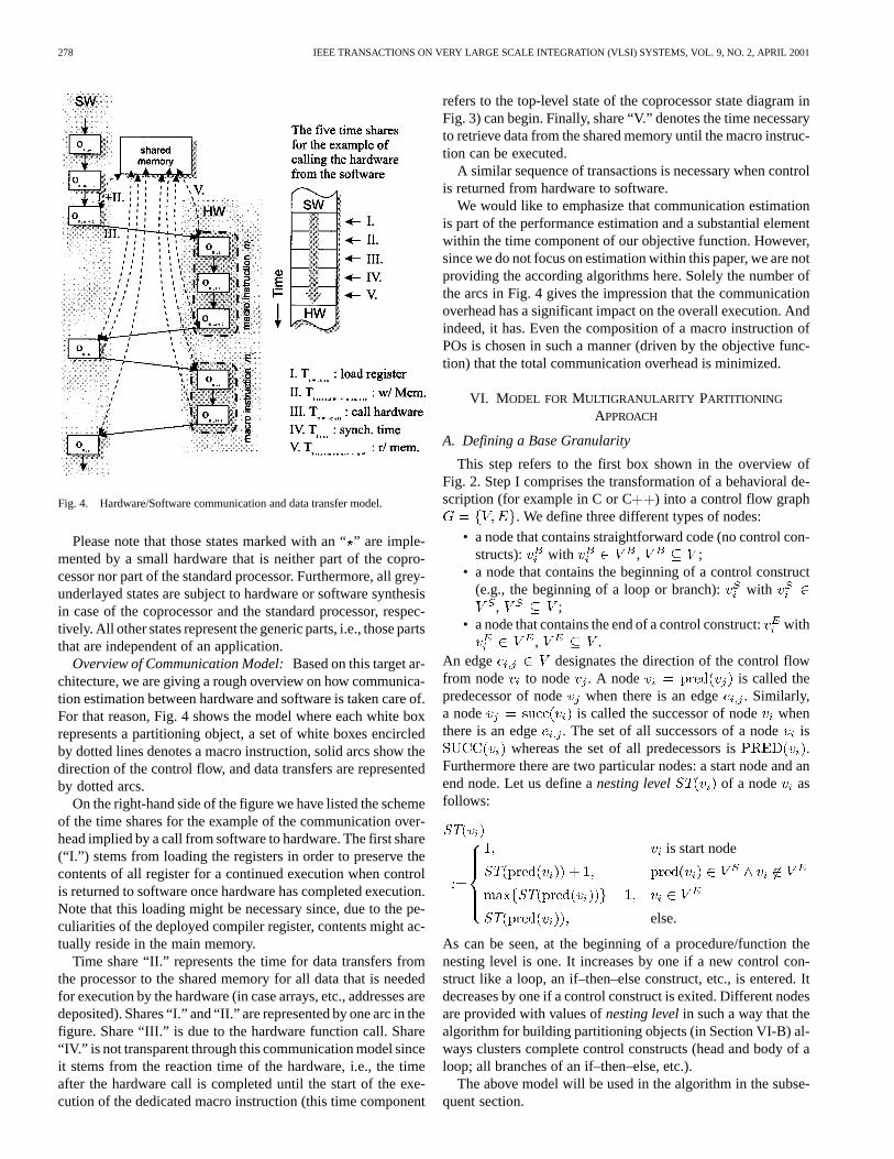
Fig. 4. Hardware/Software communication and data transfer model.

Please note that those states marked with an “” are imple-mented by a small hardware that is neither part of the copro-cessor nor part of the standard processor. Furthermore, all grey-underlayed states are subject to hardware or software synthesisin case of the coprocessor and the standard processor, respec-tively. All other states represent the generic parts, i.e., those partsthat are independent of an application.

Overview of Communication Model:Based on this target ar-chitecture, we are giving a rough overview on how communica-tion estimation between hardware and software is taken care of.For that reason, Fig. 4 shows the model where each white boxrepresents a partitioning object, a set of white boxes encircledby dotted lines denotes a macro instruction, solid arcs show thedirection of the control flow, and data transfers are representedby dotted arcs.

On the right-hand side of the figure we have listed the schemeof the time shares for the example of the communication over-head implied by a call from software to hardware. The first share(“I.”) stems from loading the registers in order to preserve thecontents of all register for a continued execution when controlis returned to software once hardware has completed execution.Note that this loading might be necessary since, due to the pe-culiarities of the deployed compiler register, contents might ac-tually reside in the main memory.

Time share “II.” represents the time for data transfers fromthe processor to the shared memory for all data that is neededfor execution by the hardware (in case arrays, etc., addresses aredeposited). Shares “I.” and “II.” are represented by one arc in thefigure. Share “III.” is due to the hardware function call. Share“IV.” is not transparent through this communication model sinceit stems from the reaction time of the hardware, i.e., the timeafter the hardware call is completed until the start of the exe-cution of the dedicated macro instruction (this time component

refers to the top-level state of the coprocessor state diagram inFig. 3) can begin. Finally, share “V.” denotes the time necessaryto retrieve data from the shared memory until the macro instruc-tion can be executed.

A similar sequence of transactions is necessary when controlis returned from hardware to software.

We would like to emphasize that communication estimationis part of the performance estimation and a substantial elementwithin the time component of our objective function. However,since we do not focus on estimation within this paper, we are notproviding the according algorithms here. Solely the number ofthe arcs in Fig. 4 gives the impression that the communicationoverhead has a significant impact on the overall execution. Andindeed, it has. Even the composition of a macro instruction ofPOs is chosen in such a manner (driven by the objective func-tion) that the total communication overhead is minimized.

VI. M ODEL FOR MULTIGRANULARITY PARTITIONING

APPROACH

A. Defining a Base Granularity

This step refers to the first box shown in the overview ofFig. 2. Step I comprises the transformation of a behavioral de-scription (for example in C or C ) into a control flow graph

. We define three different types of nodes:

• a node that contains straightforward code (no control con-structs): with , ;

• a node that contains the beginning of a control construct(e.g., the beginning of a loop or branch): with

, ;• a node that contains the end of a control construct:with

, .An edge designates the direction of the control flowfrom node to node . A node is called thepredecessor of node when there is an edge . Similarly,a node is called the successor of nodewhenthere is an edge . The set of all successors of a nodeis

whereas the set of all predecessors is .Furthermore there are two particular nodes: a start node and anend node. Let us define anesting levelST of a node asfollows:

ST

is start node

ST

ST

ST else.

As can be seen, at the beginning of a procedure/function thenesting level is one. It increases by one if a new control con-struct like a loop, an if–then–else construct, etc., is entered. Itdecreases by one if a control construct is exited. Different nodesare provided with values ofnesting levelin such a way that thealgorithm for building partitioning objects (in Section VI-B) al-ways clusters complete control constructs (head and body of aloop; all branches of an if–then–else, etc.).

The above model will be used in the algorithm in the subse-quent section.


B. Generating the Partitioning Objects

This step refers to the second box shown in the overview ofFig. 2.

Before describing the algorithm for generating the parti-tioning objects, the requirements are enlisted as follows.

a) It is desirable to put small parts like base blocks or instruc-tions into a single partitioning object.

b) Larger partitioning objects should contain whole controlconstructs (e.g., nested loops) or possibly functions/pro-cedures.

c) By means of a few moves only (a move is the action thatputs an partitioning object from software to hardware orvice versa) a “good” partitioning should be achievable.

Some definitions: we call a partitioning object. isa set that contains nodes ; hence, is a set of sets.In addition, a temporary set is deployed. It contains thosepartitioning objects that have already been generated during apreceding iteration step through the algorithm. The followingrelation holds: . In order to simplify the algorithmthe term indicates that a new partitioning objectis created by copying the contents of and to . Therein

represent partitioning objects. Finally, the algorithmfor generating the partitioning objects is formulated as follows:

1) Transform elements into partitioning objects:a)For all :If

PRED SUCC thena)b)

2) For all :a) Integrate sequential system parts:

PRED PRED

b) Integrate control constructs:PRED ST ST SUCC

succ succ

succ

c)3) updating and removing redundancy4) ready, if , else proceed with Step 2).

The algorithm is performed as long as the condition of Step4) is false. If it becomestrue, that means we have reached thelargest possible granularity (i.e., a partitioning object representsa whole function/procedure already) and no further partitioningobjects have to be created.

Note that only one of the conditions in 1), 2a), or 2b) can be-come true at one time for a newly generated partitioning objects.

The result of performing the algorithm on the example graphof Fig. 5 is depicted in Fig. 6. Each of the graphs in Fig. 6 repre-sents the state after a single iteration through the algorithm. Theresulting partitioning objects are set off by the grey color. Note

Fig. 5. Example of a graphG with corresponding source code.

that the complete set containsall meanwhile generated par-titioning objects (in the example: to ).

At this point we have defined a graph representation and analgorithm that generates partitioning objects out of the basicgranularity (that is expressed by the set). Anyhow, it is notyet clear which particular partitioning object is actually usedduring a step in hardware/software partitioning. As mentionedearlier, this might depend on the deployed estimation techniques(see Scenario 3 in Section III) and/or on the evaluation of a par-titioning through the objective function. Sections VII and VIIIare dedicated to give an answer to this question.

VII. ESTIMATION TECHNIQUES

In our approach to partitioning we use high-level estimationtechniques in order to evaluate the quality of a possible parti-tioning. In this sense, high-level estimation techniques controlthe partitioning process. Those estimation techniques comprisesoftware performance, hardware/software communicationeffort, hardware effortand power estimation. We have pro-posed appropriate techniques in [32]–[35], respectively. Herewe will describe our methodology for estimating hardwareperformance. We see which ways the granularity in partitioningand estimation can be adapted, i.e., in which way our approachto flexible granularity is controlled by the peculiarities of esti-mation techniques. Though we just demonstrate the adaptationfor our hardware performance estimation technique, similarconsiderations apply to our other estimation techniques as well.

A. Estimation Technique for Hardware Performance

Our requirements to an estimation technique for hardwareperformance as part of a partitioning approach are:

• high accuracy (compared to the actual schedule that is car-ried out by high-level synthesis after partitioning);


Fig. 6. Steps of generating the partitioning objects for an example.

• adaptation to the granularity of the partitioning process(flexible granularity);

• and the possibility of a tradeoff between computation ef-fort and quality (in order to conduct fast “what-if-anal-ysis”).

For these reasons we eventually developed a modified version ofPath-Based Scheduling[36]. The main features of our techniqueare: a sophisticated approach to control the problem ofpath ex-plosion7 while offering the possibility to adapt the partitioninggranularity and estimation granularity. The problem of path ex-plosion in Path-Based Scheduling has been addressed before by[37]–[39]. Anyhow, in contradiction to those, our approach al-lows a cost function driven decomposition of the graph. Hence,we can tradeoff between quality and computation time and wecan conduct an adaptation to any required granularity.

Path-based scheduling consists of the following passes:

I) transforming a CDFG into a directed acyclic graph;II) collecting ALL paths;III) scheduling all pathsAs-Fast-As-Possible(AFAP see

[36]);IV) overlapping all paths.

Computation time intensive Steps are III and IV as a conse-quence of Step II.

This is because the number of paths grows exponentially withthe number of nodes .

7The number of paths is2 in the worst case withN the number of nodes inthe graph that is scheduled

Fig. 7. Calculating the number of paths with different cut points set.

Our technique to circumvent the path explosion is to decom-pose the whole graph and to schedule each subgraph by itself.It should be noted that each subgraph represents a partitioningobject as defined in Section VI. Rather than describing thewhole scheduling algorithm we focus only on the decomposi-tion problem and the adaptation to partitioning (Steps I, III, andIV are the same as used in [36]).

Decomposition is conducted be setting so-calledcut points.The same graph representation as defined in Section VI is used.

We assume that each nodehas two attributes: the nestinglevelST(see Section VI) and the iteration timeit. The iterationtime it is obtained by running a profiler through the applica-tion beforewe apply our scheduling estimation. As a result ofprofiling we obtain the number of times each node of the appli-cation is performed for a typical set of input stimuli patterns.8

Before we describe our method for finding a good location forsetting cut points, we give three simple examples in order to givean idea why we defined the rules and the algorithm presentedafterwards.

Example 1: Calculating all paths in the graph representationgiven by Fig. 7 leads to a number of paths. Each path

contains a number of operations.Example 2: Now assume the graph has been split into two

subgraphs throughcut point CP1. Determining all paths for eachsubgraph leads to a total number of possible paths.

Example 3: Instead ofCP1cut pointCP2 is set and all pos-sible paths are calculated again. Here .

Examples 2 and 3 are expected to achieve a faster schedulingresult than Example 1 because acstep(control step) ends at eachcut point and a newcstepstarts right after a cut point.

The loss in quality—measured in terms of an additionalnumber of csteps—depends on thedata dependenciesofoperations before and after a cut point. Assuming that the

8The designer is responsible for providing typical input stimuli.


operations have already been optimally ordered, there is noway to influence this effect.

Another aspect is the hardware constraint (number of avail-able hardware resources like functional units). The larger thenumber of resources, the larger is the additional number of con-trol steps since a potential high parallelism is prevented (see ex-ample in Fig. 8).

A good measure for the loss of quality is the increase ofexecution time (measured in clock cycles) implied by theschedule, rather than the number of additional csteps. Letit

be the number of times an operation scheduled in control step( is the set of all control steps) is executed. Then

it (1)

gives the total execution time of a program whose graph repre-sentation has been cut into subgraphs. In spite of the factthat Example 2 and 3 lead to almost the same (reduced) numberof paths, Example 2 is expected to achieve a smaller executiontime (only fouriterations at cut pointCP1compared to ten iter-ations atCP2). These considerations lead to the formulation ofRule 1.

Rule 1: Locate the cut points at those locations in the graphthat impose a minimum number of additional clock cyclescompared to a noncut graph

(2)

Therein, and are the execution times with andwithout cut points set. Preferred candidates are those with thelowestit numbers (iterations).

Please note that possible locations for setting cut points musthave been determined before Rule 1 can be applied.

The total number of possible cut points should be reduced tothose cut points which will actually reduce the complexity (i.e.,prevent path explosion).

Rule 2: A possible cut pointCP is located after a nodeif is a join pointandif there exists a path where is the

first nodeandwhere

ST ST

Note thatST is the nesting level of node. The path endsif a node is encountered withST ST .

Fig. 9(a) shows the result after applying Rule 2 for a smallexample. There, only the location after node 5 fulfills allconditions for setting a cut point. It is obvious that cut pointsright after nodes 9 and 13 would not contribute to reducing thenumber of paths.

Now assume both Rules 1 and 2 have already been applied butthe number of cut points is too large.9 This is equivalent to a toosmall granularity (see definition of granularity in Section VI)that can lead to effects like the one described in Scenario 3 inSection III.

In that case, a reduction of cut points can be achieved by ap-plying Rule 3.

9The user determines the maximum number of paths.

Fig. 8. Comparison of schedules without (top) and with (bottom) cut pointsfor different constraints.

(a) (b)

Fig. 9. (a) Searching for possible cut points. (b) Hierarchical reducing of cutpoints.

Rule 3: Find out paths that contain more than one cut pointlocated at thesamenesting levelST. Search for that cut point thatwould partition the path into two approximately equally sizedpieces (the metric is the number of comprised operations). Inthe next step mark this cut point as “already visited” and defineit as the root of a binary tree. Afterwards, treat the resulting twopaths in the same way. Now an edge from the previous cut pointto each of the two new cut points is drawn, thus building a binarytree. The procedure is repeated for all resulting smaller pathsuntil no more cut points are found.

Cut points can now be reduced hierarchically, starting withthe cut points at the leaf of the constructed binary tree. Throughthis strategy a granularity is maintained that splits the wholegraph into equally sized pieces. Hence, the quality of the fol-lowing schedule is improved.

Note that the user determines the total number of cut pointsthat are actually set. The algorithm above gives a precedence


Fig. 10. Path-based estimation technique applying rule 1 to 3.

only, i.e., it determines which cut point to delete next. An ex-ample is given in Fig. 9.

Fig. 10 shows in which way Rules 1 to 3 are applied withinour performance estimation technique (we call itpath-based es-timation technique): It starts with initializing the set of cut pointswith the empty set. Afterwards profiling data (it values) is gen-erated (by simulation) and written to the graph representation.In the following step the graph is transformed into a directedacyclic graph (DAG) and the number of all paths #pathsis com-puted (lines 2–5). If the number of paths would exceed the com-putation time (Table I says that a number of leads to ac-ceptable computation time of a few minutes only) cut points arecalculated (l.7, l.15ff, see below). Then the DAG is split at theaccording locations (l.8) and for all dag’s in a path-basedscheduling is executed. First all paths are calculated and for eachpath anAFAP-schedule is performed (l. 9–13). Then the set ofall constraints is taken in order to superimpose all constraintsof all paths (l. 14). Cut points are computed in the functioncom-pute cutpoints. It starts with scanning all nodes of the DAG(l. 17). If a node fulfills the conditions formulated by Rule 1,the node is inserted in the list of potential cut pointsCP list (l.18, 19). Now the cut points are sorted in such a way that thosecut points which are located at less often executed parts of thegraph (i.e., low iteration time ) have the highest priority since

TABLE IBENCHMARKS SCHEDULED WITH PATH-BASED ESTIMATION TECHNIQUEUSING

4 ALUS, 4 MULTIPLIERS

they lead to the smallest deviation from the optimum schedule(l. 20).

At this point the user can determine the quality-/computation-time-tradeoff by choosing the number of cut points to apply (l.21). If the number of potential cut points found exceeds thisnumber (l. 22) a selection is necessary: for the case there aremore than one cut points in the list which would lead to thesame loss of quality—assuming only Rule 1 and 2 have beenapplied—Rule 3 will decide (l. 23, 24) which of them will bedeleted from the list in order to meet exactly the user-defined# .

B. Adaptation of Estimation and Granularity

As we already mentioned briefly, the granularity for parti-tioning depends on the results of the Estimation. In the followingthis dependency is explained.

The point is that we cannot consider those partitioning objects(POs) for which we cannot provide an appropriate estimation.Assume, for instance,Example 2from Section VII-A where cutpoint number 1 is set. Assume furthermore that our algorithmfrom Section VI-B proposes a PO that comprises four nodes

. Now we would need to have a path thatsolely comprises nodes that are also part of in order toprovide with an estimation value. Obviously, there is nosuch path in the whole path set . Consequently, wehave no estimation value for it. It also does not help that paths

overlap with partitioning object .


Fig. 11. Computation time (using a SPARC20) versa number of cut points.

In a similar discussion we could construct an example wherewe have a large PO (meaning it comprises many nodes) thatwould require too many (since small) paths in order to get es-timated. Estimation actually would have to be accomplishedthrough “patching” what is not acceptable since it is too inac-curate. The latter case can happen if we chose many cut pointsresulting in many small paths. Concludingly, in both exampleswe cannot estimate the according POs. As a result those POswill not be considered, i.e., they will actually be deleted from

(see Section VI-B).Obviously, the estimation method controls the possible gran-

ularity: if we chose many cut points then many small paths areobtained such that finally small POs are selected. If we chosea few cut points only, accordingly large POs are preferred. Orin a more general manner: the quality we prefer for estimationdirectly influences the possible granularity.

C. Results Achieved by Deploying the Hardware PerformanceEstimation Technique

Table I shows the results achieved by our performance esti-mation technique. For diverse applications, the number of paths(#pth), the number of cut points (#cpt), the scheduling result,and the computation time are given. Note that the user deter-mines the number of cut points he/she wants to be set. Thus, thequality/computation time tradeoff is influenced: if only a fewcut points are set, the number of paths is higher, the computa-tion time increase but the quality of the schedule is improved.The other way around, many cut points lead to fewer paths, thecomputation time is decreased, but the quality of the schedulesuffers. More apparent than these pure numbers, Figs. 11 and12 unveil a peculiar behavior that we can exploit to optimizethe quality/computation time tradeoff: interestingly, Fig. 11 un-veils that the computation times decreases steeply with a fewcut points set but at a certain point, an additional number of cutpoints leads to an unremarkable improvement in computationtime (those points are marked by arcs).

An accuracy of the schedule of about 15% (given in Fig. 12 asa deviation in percent compared to the best possible schedule)can already be achieved at a small fraction of all paths. Or wecan argue the other way around: if we would consider morepaths in order to perform the schedule then we would signifi-cantly increase the computation while the accuracy would in-

Fig. 12. Tradeoff between quality (deviation from according best schedule)and complexity (number of paths).

crease only insubstantially. Our conclusion is that the best com-promise between quality and computation time is to consideronly a fraction of all paths. This is possible through our methodthat sets cut points accordingly.

VIII. O PTIMIZATION THROUGH A DYNAMICALLY WEIGHTED

OBJECTIVE FUNCTION

The task of the optimization algorithm is to find the best hard-ware/software partition according to an objective function. Asmentioned earlier, our definition of amacro functionis the actualimplementation of a piece of hardware in form of an applicationspecific hardware (ASIC). A macro function will typically con-sist of a set of consecutive partitioning objects. A large varietyof different granularities (differently sized partitioning objects)supports the optimization algorithm in finding a good partition.Or in other words, if a large macro instruction would lead to agood partition but onlysmallpartitioning objects are available,manyof them would be needed. Thus optimization becomesmore complex and finding that specific good solution is moreunlikely. Hence, a flexible granularity enhances the prospect toobtain good results, i.e., partitions.

This step refers to the third box shown in the overview ofFig. 2.

As an optimization algorithm we have chosen the simulatedannealing algorithm [40]. The reasons are as follows.

• It is mathematically well investigated.• It offers the possibility of a quality/computation time

tradeoff.• It is a general-purpose optimization algorithm (that means

it is easy to adapt to our partitioning model).Our implementation uses theannealing scheduledescribed in[41] since it offers one of the best quality/computation timetradeoffs. The interface between the annealing schedule and ourspecific problem formulation of partitioning consists of basi-cally three functions:

• generate()When this function is called the generation of a new stateis requested, i.e., in hardware/software partitioning a newpartition has to be generated. This is done by a move


of a partitioning object from software to hardware or viceversa. A characteristic peculiarity of each partitionis itscostCost . Thereby is the set of all possiblepartitions.

• accept()If the annealing algorithm has decided to accept a movethenaccept() returns the value “TRUE”.

• reject()If the annealing algorithm has decided not to accept thismove thenreject() returns the value “TRUE”.

A. Selection of a Move

The following prerequisites led to the definition of the selec-tion algorithm for a new move:

• Exactly one partitioning object is moved from software tohardware or vice versa during one call of thegenerate()function.

• The algorithm assumes that hardware and software partsexecute in mutual exclusion.10

• The algorithm should select a new move dependent uponthe current partition.

Within the following algorithm the term has themeaning that partitioning object is moved from softwareto hardware using the move . The algorithm is defined asfollows:

1) Random selection of an object2) Case 1: Selected object is in SW

If

Then

a) Valid move:

3) Case 2: Selected object is in HWIf

Thena) If

ThenNo move possible. Proceed with 1) above

Else

Valid move:

4) Case 3: Selected object is in parts in SW and in parts in HWIf

Thena)

b)

c) Valid move:

10This is because our target architecture is constrained to that model. Anyhow,our algorithm needs only slightly changes to be applicable for a concurrent ex-ecution of hardware and software. In this sense, the methodologies presented inthis paper are very generally applicable.

Fig. 13. All possible base configurations and characteristic moves.

5) IfNone of the conditions in steps 2), 3), 4) is fulfilled

ThenProceed with 2) above

ElseReady, since a valid move is found.

If a valid move is found, exactly one of the cases Case 1, Case2, or Case 3 will be applied. All possible base configurationsand moves are depicted in Fig. 13. The assignments of cases tofigures are as follows:

• Case 1 “TRUE” corresponds to Fig. 13(a);• Case 2 a) “FALSE” corresponds to Fig. 13(b);• Case 2 a) “TRUE” corresponds to Fig. 13(c);• Case 3 “TRUE” corresponds to Fig. 13(d).

A situation like the one in Fig. 13(e) cannot occur since no movecan generate such an initial configuration (it would hurt the con-ventions on the target architecture, i.e., mutual exclusive execu-tion of software and hardware). Based on this base configura-tions and according moves every valid codesign can be reached.

B. Partitioning and Granularity

In Section VIII-A we have shown in which way the estimationalgorithm influences the possible granularity. Here, we explainin which way a flexible granularity finally leads to (small orlarge) macro instructions.

During each move of the optimization algorithm, one par-titioning object is finally selected and supposed to be imple-mented as hardware or as software (see algorithm is previoussection). Let us assume, for example, that the final implemen-tation is likely to have many hardware parts and a few softwareparts (this might be the case when severe timing constraints are


imposed that can only be met when the hardware part is large).In this case it is obviously more advantageous if the algorithmwould select larger partitioning objects rather than smaller. Butsince a partitioning object is selected randomly (we use Simu-lated Annealing), we cannot influence the selection itself. Butonce one of the large partitioning objects has been selected ran-domly, it may significantly improve the cost function. The otherway around, a small partitioning object that is selected to be re-moved from the hardware side will less insignificantly aggravatethe cost function than a large one would. As a consequence, theoptimization algorithm will implicitly tend to collect a few butlarge partitioning objects for hardware implementation insteadof many small. This leads to a smaller number of moves. Otherexamples can be constructed where a large partitioning objectwould be too expensive and a few small can achieve a better re-sult.

Thus, the flexible granularity helps to achieve:

• better hardware/software designs;• to reduce the computation time during partitioning.

All adjacent partitioning objects (those that provide a con-tiguous part in the control flow) that finally have been selectedfor a hardware implementation form one macro instruction.Typically, more than one macro instructions is implemented.

C. Multilevel Objective Function

The task of the objective function is to measure the qualityof the partition after each move that has been proposed by theoptimization algorithm. The problem in defining a objectivefunction is to find a appropriate way to tradeoff different designgoals/constraints against each other. Design constraints/goalsare: performance, hardware effort, power dissipation, etc.Though the ideas of our objective function are general wedemonstrate the usefulness by means of one design constraint(performance) and one optimization goal (hardware effort).

The objective function is defined as follows:

cost (3)

We will discuss the single components in the following, es-pecially the weighting factor which varies dynamically,dependent on how close the time constraint is met. A staticweighting by using the two constant factorsand only is notsufficient for our purpose of meeting a real-time constraintandminimizing the hardware effort at the same time. But before, letus discuss another problem: sincetimeandareahave differentphysical units, we have to normalize our components. As for thehardware component, we calculate the area of a piece of hard-ware (using our estimation method presented in Section VII)and divide it by the average area of all other pieces of hardware

. Consequently, we get a relative number that is in averageclose to 1.

The time component is normalized as follows:

Fig. 14. Factorw as a finction ofT .

Here, is the real-time constraint and is the currentexecution time of the system. Since our aim is

we define the deviation as a cost and put it inrelation to in order to get a unit-less number that can becombined with the area component. The constant 1 is added forthe case where , meaning that in that case the areacomponent would totally dominate unless we add 1.

So far, the cost function has been built straightforward. How-ever, we would never gain our aim of meeting a real-time con-straint and minimizing the hardware effort unless we would careabout . A desirable behavior of would be that it iszero when we are far away from meeting the real-time con-straint. This means that in such cases the timing behavior isoptimized exclusively. But when is close to , thearea component should start to become more and more influ-ence until is almost equal to where should bemaximum. This is a dynamic weighting, meaning that isdependent on the timing component. The following definitionfulfills the desirable behavior:

else

The value of is obtained by experience. In a more apparentway, is shown in Fig. 14. Actually there are given threepossible examples of how can look like depending on theparameter . For a small value of the outermost flanksapply. For large values of (indicated by the direction thearcs are heading to) the innermost flanks apply. The flanks be-tween belong to a value of that is somewhere between. Un-less the system timing is far away from .If is close to starts to increase until itbecomes maximum (i.e., 1). Now the area component is domi-nating over the time component. This is desirable since the timeconstraints at this stage has almost been fulfilled. So, the dy-namic weighting offers the possibility of separating area and


time dependent on the current state, without switching to an-other objective function (this might be very computation inten-sive). By means of the factors and in (3) it is possible tocontrol the extent to which the area component should domi-nate during the end-phase of the optimization procedure.

We want to emphasize that our objective function is notthe first one to comprise performanceand area. In fact,Vahid/Gajski [13] propose an objective function by formulatingthe violations in terms of timing and area. But the weighingbetween these violations is fixeda priori. An adaptation ofthe weighing between the violations, according to the currentstate of the partitioning process, is not provided. This is wherewe see the advantage of our approach that does provide thisflexibility.

Kalavade/Lee [20] propose another approach to meet timingconstraintsand minimize hardware during hardware/softwarepartitioning. They divide their optimization algorithm into twophases. One is for meeting the timing constraints solely. Oncethis is accomplished they switch to a second phase where theytake care of area minimization. In our approach we do not haveto switch between two different optimization phases. Instead,the weighing between timing component and area componentvariescontinuously. Thus we avoid a possibly nondeterminedbehavior of the optimization algorithm due to abrupt switching.

As we will show in the following section, our flexible ap-proach achieves significantly better results than our previouslydeployed approach that featured an objective function with fixedweighing factors.

IX. EXPERIMENTS AND RESULTS

Experiments have been conducted in order to show the su-periority of our hardware/software partitioning approach with aflexiblegranularity compared to an approach with afixedgran-ularity. We will also show the efficiency of our multilevel ob-jective function. As for the performance estimation technique,we already presented results in Section VII.

Most of the applications stem from the domain of digitalsignal processing and some others are control dominated. Thepartitioning approach with flexible granularity is applicable toboth domains as the results will show. The size of the applica-tions vary from about 50 lines of C code to about 600 lines of Ccode and the number of paths ranges from 28 to 18.5 Mio. Oneof the applications is part of a real industrial project. Throughthis diversity of sizes the partitioning approach can show that aflexible granularity leads to fastandhigh-quality results, inde-pendent from the size of the applications. It should be noted thatwe used the same applications in the experiments in Section VIIas we did for partitioning here in this section. But in Section VIIwe used single functions of the particular application whereaswe usedwholeapplications consisting of one or more functionshere.

The results have been achieved by a fully automated parti-tioning algorithm and estimation techniques.

The quality of our approach is evaluated by means of theachievedspeedup, thehardware effortof the applications spe-cific hardware, and thecomputation timeof our algorithm.

Fig. 15. Speedup constraintspu and estimated speedupspu fordifferent design points of an application.

A. Speedup

Thespeedupis defined as

spu spu

where is the execution time of an application for anall-software solution, is the execution time of thesame application but for a hardware/software implementation(after partitioning), andspu is the imposed constraintspeedup. Fig. 15 shows the behavior of the obtained speedupand speedup constraint for different design points of an ap-plication. The graph “spu ” gives the result obtained by thepartitioner. It can be seen that in all cases the constraint of theabove equation is metspu spu .

Table II shows some more results. It also shows the realspeedup “spu ” that has been achieved as follows: after hard-ware/software partitioning the software part has been mappedto a standard processor core (SPARC) and the hardware part(including interfaces) has been synthesized using high-levelsynthesis. Afterwards we have taken the output (slif netlist) ofthe high-level synthesis and optimized it using the SYNOPSYSdesign compiler. After simulation of software and hardwareparts we got the real speedup called “spu .”

The table shows that in all cases the speedup values are veryclose to the constraint. The partitioner meets the given speedupconstraint in all cases. Due to the inaccuracy of the estima-tion tools (hardware run-time, software run-time, communica-tion time) that perform estimation at a high level of abstractionthere are some small deviations between real synthesis resultsspu and constraintspu . That reflects that the estima-

tion tools are of good accuracy.An arc in the table has the meaning that the according design

point is the same as the one the arc points to. Other applicationscannot be sped up more than a maximum value due to the pecu-liarities of an application and the deployed hardware resources.

B. Hardware Effort

Since embedded systems on a chip are limited in size, min-imizing the hardware effort is an important goal. The attribute


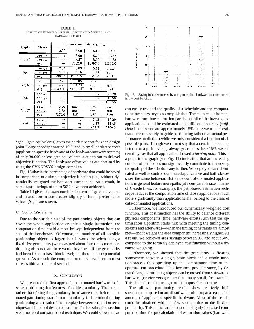
TABLE IIRESULTS OFETIMATED SPEEDUP, SYNTHESIZED SPEEDUP, AND

HARDWARE EFFORT

“geq” (gate equivalents) gives the hardware cost for each designpoint. Large speedups around 10.0 lead to small hardware costs(application specific hardware of the hardware/software system)of only 30.000 or less gate equivalents is due to our multilevelobjective function. The hardware effort values are obtained byusing the SYNOPSYS design compiler.

Fig. 16 shows the percentage of hardware that could be savedin comparison to a simple objective function (i.e., without dy-namically weighted the hardware component. As a result, insome cases savings of up to 50% have been achieved.

Table III gives the exact numbers in terms of gate equivalentsand in addition in some cases slightly different performancevalues are shown.

C. Computation Time

Due to the variable size of the partitioning objects that cancover the whole application or only a single instruction, thecomputation time could almost be kept independent from thesize of the benchmark. Of course, the number of all possiblepartitioning objects is larger than it would be when using afixed-size granularity (we measured about four times more par-titioning objects than there would have been if the granularityhad been fixed to base block level; but there is no exponentialgrowth). As a result the computation times have been in mostcases within a couple of seconds.

X. CONCLUSION

We presented the first approach to automated hardware/soft-ware partitioning that features a flexible granularity. That meansrather than fixing the granularity in advance (i.e., before auto-mated partitioning starts), our granularity is determined duringpartitioning as a result of the interplay between estimation tech-niques and imposed design constraints. In the estimation sectionwe introduced our path-based technique. We could show that we

Fig. 16. Saving in hardware cost by using an explicit hardware cost componentin the cost function.

can easily tradeoff the quality of a schedule and the computa-tion time necessary to accomplish that. The main result from thehardware run-time estimation part is that all of the investigatedapplications could be estimated at a sufficient accuracy (suffi-cientin this sense are approximately 15% since we use the esti-mation results solely to guide partitioning rather than actual per-formance prediction) while we only considered a fraction of allpossible parts. Though we cannot say that a certain percentagein terms of a path coverage always guarantees these 15%, we cancertainly say that all application showed aturning point. This isa point in the graph (see Fig. 11) indicating that an increasingnumber of paths does not significantly contribute to improvingthe quality of the schedule any further. We deployed data-domi-nated as well as control-dominated applications and both classesshow the same behavior. But since control-dominated applica-tions in general feature more paths (at a comparable size in termsof C-code lines, for example), the path-based estimation tech-nique reduces the computation time of those applications muchmore significantly than applications that belong to the class ofdata-dominated applications.

Furthermore, we introduced our dynamically weighted costfunction. This cost function has the ability to balance differentphysical components (time, hardware effort) such that the op-timization algorithm starts first with meeting the timing con-straints and afterwards—when the timing constraints are almostmet—and it weighs the area component increasingly higher. Asa result, we achieved area savings between 0% and about 50%compared to the formerly deployed cost function without a dy-namic weighing.

Furthermore, we showed that the granularity is floatingsomewhere between a single basic block and a whole func-tion/process thus speeding up the computation time of theoptimization procedure. This becomes possible since, by de-mand, large partitioning objects can be moved from software tohardware (or vice versa) rather than many small, for example.This depends on the strenght of the imposed constraints.

The all-over partitioning results show relatively highspeedups (compared to an all-software solution) at a reasonableamount of application specific hardware. Most of the resultscould be obtained within a few seconds due to the flexiblegranularity. This comes at the cost of a slightly increased com-putation time for precalculation of estimation values (hardware


TABLE IIIHARDWARE EFFORTUSING THE DYNAMICALLY WEIGHTED COST FUNCTION AS OPPOSED TO ACOST FUNCTION WITHOUT DYNAMIC WEIGHTING

OF THE HARDWARE COMPONENT

performance, etc.) since the number of all derived partitioningobjects (please remember that they may overlap) is alwayslarger than the number of all base blocks. But this disadvantageis by far outweighed by the speed of the partitioning processusing the flexible granularity, especially when it comes tolarge applications. An open issue for future work could be tointegrate an additional component (like power, for example)into the cost function and to handle the mutual dependencies ofperformanceandareaandpower.

REFERENCES

[1] J. Henkel and R. Ernst, “A hardware/software partitioner using a dy-namically determined granularity,” inIEEE/ACM Proc. 34th Design Au-tomation Conf., 1997, pp. 691–696.

[2] A. W. Aho, R. Sethi, and J. D. Ullmann,COMPILERS Principles, Tech-niques and Tools: Bell Telephone Lab., 1987.

[3] R. Gupta and Y. Zorian, “Introducing core-based system design,”IEEEDesign Test Mag., vol. 13, pp. 15–25, Dec. 1997.

[4] C. Kuttner, “Hardware-software codesign using processor synthesis,”IEEE Design Test Computers, vol. 13, pp. 43–53, 1996.

[5] P. Athanas and H. F. Silverman, “Processor reconfiguration through in-struction-set metamorphosis,”IEEE Computer Mag., pp. 11–18, Mar.1993.

[6] E. Barros, W. Rosenstiel, and X. Xiong, “A Method for partitioningUNITY language in hardware and software,” inProc. IEEE/ACM Proc.European Conf. Design Automation (EuroDAC), 1994, pp. 220–225.

[7] A. Jantsch, P. Ellervee, and J. Oeberget al., “Hardware/software parti-tioning and minimizing memory interface traffic,” inIEEE/ACM Proc.European Conf. Design Automation (EuroDAC), 1994, pp. 220–225.

[8] P. V. Knudsen and J. Madsen, “PACE: A dynamic programming algo-rithm for hardware/software partitioning,” inIEEE/ACM Proc. 4th Int.Workshop Hardware/Software Codesign, 1996, pp. 85–92.

[9] M. F. Parkinson and S. Parameswaran, “Profiling in the ASP codesignenvironment,” inIEEE/ACM Proc. 8th Int. Symp. System Synthesis,1995, pp. 128–133.

[10] R. Ernst, J. Henkel, and T. Benner, “Hardware/software co-synthesis formicrocontrollers,”IEEE Design Test Mag., vol. 10, Dec. 1993.

[11] M. Edwards and J. Forrest, “A development environment for the cosyn-thesis of embedded software/hardware systems,” inIEEE/ACM Proc.EDAC’94, 1994, pp. 469–473.

[12] Z. Peng and K. Kuchcinski, “An algorithm for partitioning of applicationspecific system,” inIEEE/ACM Proc. European Conf. Design Automa-tion (EuroDAC), 1993, pp. 316–321.

[13] F. Vahid, D. D. Gajski, and J. Gong, “A binary-constraint search algo-rithm for minimizing hardware during hardware/software partitioning,”in IEEE/ACM Proc. European Conf. Design Automation (EuroDAC),1994, pp. 214–219.

[14] F. Vahid and D. D. Gajski, “Clustering for improved system-level func-tional partitioning,” inIEEE/ACM Proc. 8th Int. Symp. System Synthesis,1995, pp. 28–33.

[15] J. K. Adams and D. E. Thomas, “Multiple-process behavioral synthesisfor mixed hardware-software systems,” inIEEE/ACM Proc. 8th Int.Symp. System Synthesis, 1995, pp. 10–15.

[16] P. H. Chou, R. B. Ortega, and G. B. Borriello, “The Chinook hard-ware/software co-synthesis system,” inIEEE/ACM Proc. 8th Int. Symp.System Synthesis, 1995, pp. 22–27.

[17] J. G. D’Ambrosio and X. Hu, “Configuration-level hardware/softwarepartitioning for real-time embedded systems,” inProc. 3rd IEEE Int.Workshop Hardware/Software Codesign, 1994, pp. 34–41.

[18] C. Carreras, J. C. Lopez, and M. L. Lopezet al., “A co-design method-ology based on formal specification and high-level estimation,” inProc.4th IEEE Int. Workshop Hardware/Software Codesign, 1996, pp. 28–35.

[19] T. B. Ismail, M. Abid, and A. Jerraya, “COSMOS: A co-design approachfor communicating system,” inIEEE/ACM Proc. 3rd IEEE Int. Work-shop Hardware/Software Codesign, 1994, pp. 17–24.

[20] A. Kalavade and E. Lee, “A global critically/local phase drivenalgorithm for the constraint hardware/software partitioning problem,”in Proc. 3rd IEEE Int. Workshop Hardware/Software Codesign, 1994,pp. 42–48.

[21] A. Balboni, W. Fornaciari, and D. Sciuto, “Partitioning and explorationstrategies in the TOSCA co-design flow,” inProc. 4th IEEE Int. Work-shop Hardware/Software Codesign, 1996, pp. 62–69.

[22] J. Teich, T. Bickle, and L. Thiele, “An evolutionary approach to system-level synthesis,” inProc. 5th IEEE Int. Workshop Hardware/SoftwareCodesign, 1997, pp. 167–171.

[23] T. Y. Yen and W. Wolf, “Multiple-process behavioral synthesis for mixedhardware-software systems,” inIEEE/ACM Proc. 8th Int. Symp. SystemSynthesis, 1995, pp. 4–9.

[24] R. K. Gupta and G. D. Micheli, “System-level synthesis using re-pro-grammable components,” inIEEE/ACM Proc. EDAC’92, 1992, pp. 2–7.

[25] R. Niemann and P. Marwedel, “Hardware/software partitioning using in-teger programming,” inIEEE/ACM Proc. EDAC’96, 1996, pp. 473–479.

[26] D. Kirovski and M. Potkonjak, “System-level synthesis of low-powerhard real-time systems,” inIEEE/ACM Proc. 4th DAC’97, 1997, pp.697–702.

[27] B. P. Dave, G. Lakshminarayana, and N. K. Jha, “CoSYN: Hardware-software co-synthesis of embedded systems,” inIEEE/ACM Proc. 34thDAC’97, 1997, pp. 703–708.

[28] J. Henkel and Y. Li, “Energy-conscious HW/SW-partitioning of em-bedded systems: A case study on an MPEG-2 encoder,” inIEEE/ACMProc. 6th Int. Workshop Hardware/Software Codesign, 1998, pp. 23–27.

[29] F. Balarin, M. Chiodo, and D. Engelset al., “POLIS: A design envi-ronment for control-dominated embedded systems,” Internal Rep., UCBerkeley, 1996.

[30] B. Lin, “A system design methodology for software/hardware co-de-velopment of telecommunication network applications,” inIEEE/ACMProc. 33rd Design Automation Conf. (DAC), 1996, pp. S. 672–677.

[31] K. Buchenrieder and C. Veith, “CODES: A practical concurrent designenvironment,” inHandout Int. Workshop Hardware-Software Co-De-sign, Estes Park, CO, Oct. 1992.

[32] W. Ye, R. Ernst, Th. Benner, and J. Henkel, “Fast timing analysis forhardware-software co-synthesis,” inProc. ICCD, 1993, pp. 452–457.

[33] J. Henkel, Th. Benner, R. Ernst, W. Ye, N. Serafimov, and G. Glawe,“COSYMA: A software-oriented approach to hardware/software code-sign,” J. Computer Software Eng., vol. 2, no. 3, pp. 293–314, 1994.

[34] J. Henkel and R. Ernst, “High-level estimation techniques for usagein hardware/software co-design,” inIEEE Proc. Asia South PacificDAC’98, 1998, pp. 353–360.

[35] Y. Li and J. Henkel, “A framework for estimating and minimizing energydissipation of embedded HW/SW systems,” in35th Design AutomationConf. (DAC), San Francisco, CA, June 1998.

[36] R. Camposano, “Path-based scheduling for synthesis,”IEEE Trans.Computer-Aided Design, vol. 10, pp. 85–93, Jan. 1991.

[37] K. O’Brien, M. Rahmouni, and A. Jerraya, “DLS: A scheduling algo-rithm for high-level synthesis in VHDL,” inProc. EDAC’93, 1993, pp.393–397.

[38] M. Rahmouni and A. Jerraya, “PPS: A pipeline path-based scheduler,”in Proc. EDAC’95, 1995, pp. 557–561.

[39] R. A. Bergamaschi, S. Raje, I. Nair, and L. Trevillyan, “Control-flowversus data-flow-based scheduling: Combining both approaches in anadaptive scheduling system,”IEEE Trans. VLSI Syst., vol. 5, pp. 82–100,Mar. 1997.

[40] R. Otten and P. V. Ginneken,The Annealing Algorithm: Kluwer, 1989.[41] J. Lam and J.-M. Delosme, “Performance of a new annealing schedule,”

in IEEE/ACM Proc. 25th Design Automation Conf. (DAC), 1988, pp.306–311.


Jörg Henkel (M’98–SM’00) received the diploma inelectrical engineering in 1991 and the Ph.D. degree in1996 both from the Technical University of Braun-schweig, Germany.

Since 1997 he has been working as a ResearchStaff Member at the Computer & CommunicationResearch Labs at NEC in Princeton, NJ. In Spring2000 he was a Visiting Professor at the Universityof Notre Dame, IN. Besides hardware/softwareco-design (he is a Program Co-Chair of IEEE/ACMInternational Symposium of Hardware/Software

Co-Design CODES’01) his interests include embedded system design method-ologies.

Rolf Ernst (M’95) received the diploma in computerscience in 1981 and the Ph.D. degree in electrical en-gineering in 1988, both from the University of Er-langen-Nuremberg, Germany.

From 1988 to 1989, he was a Member of TechnicalStaff at Bell Labs in Allentown, PA. Since 1990, hehas been a Professor at the Technical University ofBraunschweig, Germany. His main research interestsare in embedded system design and embedded systemdesign automation.

Dr. Ernst is a member of ACM and the German GI.

an approach to automated hardware/software partitioning ... · pdf filehardware/software...

Documents