an application to transportation engineering by s.n.lahiri …
TRANSCRIPT

arX
iv:1
301.
2459
v1 [
stat
.AP]
11
Jan
2013
The Annals of Applied Statistics
2012, Vol. 6, No. 4, 1552–1587DOI: 10.1214/12-AOAS587c© Institute of Mathematical Statistics, 2012
GAP BOOTSTRAP METHODS FOR MASSIVE DATA SETS WITHAN APPLICATION TO TRANSPORTATION ENGINEERING1
By S. N. Lahiri, C. Spiegelman, J. Appiah and L. Rilett
Texas A&M University, Texas A&M University, University of
Nebraska-Lincoln and University of Nebraska-Lincoln
In this paper we describe two bootstrap methods for massive datasets. Naive applications of common resampling methodology are of-ten impractical for massive data sets due to computational burdenand due to complex patterns of inhomogeneity. In contrast, the pro-posed methods exploit certain structural properties of a large class ofmassive data sets to break up the original problem into a set of sim-pler subproblems, solve each subproblem separately where the dataexhibit approximate uniformity and where computational complexitycan be reduced to a manageable level, and then combine the resultsthrough certain analytical considerations. The validity of the pro-posed methods is proved and their finite sample properties are stud-ied through a moderately large simulation study. The methodology isillustrated with a real data example from Transportation Engineer-ing, which motivated the development of the proposed methods.
1. Introduction. Statistical analysis and inference for massive data setspresent unique challenges. Naive applications of standard statistical method-ology often become impractical, especially due to increase in computationalcomplexity. While large data size is desirable from a statistical inference per-spective, suitable modification of existing statistical methodology is neededto handle such challenges associated with massive data sets. In this paper,we propose a novel resampling methodology, called the Gap Bootstrap, fora large class of massive data sets that possess certain structural properties.The proposed methodology cleverly exploits the data structure to breakup the original inference problem into smaller parts, use standard resam-pling methodology to each part to reduce the computational complexity,
Received April 2012.1Supported in part by grant from the U.S. Department of Transportation, University
Transportation Centers Program to the University Transportation Center for Mobility(DTRT06-G-0044) and by NSF Grants no. DMS-07-07139 and DMS-10-07703.
Key words and phrases. Exchangeability, multivariate time series, nonstationarity, ODmatrix estimation, OD split proportion, resampling methods.
This is an electronic reprint of the original article published by theInstitute of Mathematical Statistics in The Annals of Applied Statistics,2012, Vol. 6, No. 4, 1552–1587. This reprint differs from the original in paginationand typographic detail.
1

2 LAHIRI, SPIEGELMAN, APPIAH AND RILETT
and then use some analytical considerations to put the individual piecestogether, thereby alleviating the computational issues associated with largedata sets to a great extent.
The class of problems we consider here is the estimation of standard er-rors of estimators of population parameters based on massive multivariatedata sets that may have heterogeneous distributions. A primary example isthe origin-destination (OD) model in transportation engineering. In an ODmodel, which motivates this work and which is described in detail in Sec-tion 2 below, the data represent traffic volumes at a number of origins anddestinations collected over short intervals of time (e.g., 5 minute intervals)daily, over a long period (several months), thereby leading to a massive dataset. Here, the main goals of statistical analysis are (i) uncertainty quantifi-cation associated with the estimation of the parameters in the OD modeland (ii) to improve prediction of traffic volumes at the origins and the desti-nations over a given stretch of the highway. Other examples of massive datasets having the required structural property include (i) receptor modelingin environmental monitoring, where spatio-temporal data are collected formany pollution receptors over a long time, and (ii) toxicological models fordietary intakes and drugs, where blood levels of a large number of toxins andorganic compounds are monitored in repeated samples for a large number ofpatients. The key feature of these data sets is the presence of “gaps” whichallow one to partition the original data set into smaller subsets with niceproperties.
The “largeness” and potential inhomogeneity of such data sets presentchallenges for estimated model uncertainty evaluation. The standard prop-agation of error formula or the delta method relies on assumptions of in-dependence and identical distributions, stationarity (for space–time data)or other kinds of uniformity which, in most instances, are not appropriatefor such data sets. Alternatively, one may try to apply the bootstrap andother resampling methods to assess the uncertainty. It is known that theordinary bootstrap method typically underestimates the standard error forparameters when the data are dependent (positively correlated). The blockbootstrap has become a popular tool for dealing with dependent data. Byusing blocks, the local dependence structure in the data is maintained and,hence, the resulting estimates from the block bootstrap tend to be less bi-ased than those from the traditional (i.i.d.) bootstrap. For more details,see Lahiri (1999, 2003). However, computational complexity of naive blockbootstrap methods increases significantly with the size of the data sets, asthe given estimator has to be computed repeatedly based on resamples thathave the same size as the original data set. In this paper, we propose two re-sampling methods, generally both referred to as Gap Bootstraps, that exploitthe “gap” in the dependence structure of such large-scale data sets to reducethe computational burden. Specifically, the gap bootstrap estimator of the
GAP BOOTSTRAP FOR MASSIVE DATA SETS 3
standard error is appropriate for data that can be partitioned into approxi-mately exchangeable or homogeneous subsets. While the distribution of theentire data set is not exchangeable or homogeneous, it is entirely reasonablethat many multivariate subsets will be exchangeable or homogeneous. If theestimation method that is being used is accurate, then we show that thegap bootstrap gives a consistent and asymptotically unbiased estimate ofstandard errors. The key idea is to employ the bootstrap method to each of
the homogeneous subsets of the data separately and then combine the esti-
mators from different subsets in a suitable way to produce a valid estimator
of the standard error of a given estimator based on the entire data set. Theproposed method is computationally much simpler than the existing resam-pling methods that require repeated computation of the original estimator,which may not be feasible simply due to computational complexity of theoriginal estimator, at the scale of the whole data set.
The rest of the paper is organized as follows. In Section 2 we describe theOD model and the data structure that motivate the proposed methodology.In Section 3 we give the descriptions of two variants of the Gap Bootstrap.Section 4 asserts consistency of the proposed Gap Bootstrap variance esti-mators. In Section 5 we report results from a moderately large simulationstudy, which shows that the proposed methods attain high levels of accuracyfor moderately large data sets under various types of gap-dependence struc-tures. In Section 6 we revisit the OD models and apply the methodology toa real data set from a study of traffic patterns, conducted by an intelligenttraffic management system on a test bed in San Antonio, TX. Some con-cluding remarks are made in Section 7. Conditions for the validity of thetheoretical results and outlines of the proofs are given in the Appendix.
2. The OD models and the estimation problem.
2.1. Background. The key component of an origin-destination (OD) mod-el is an OD trip matrix that reflects the volume of traffic (number of trips,amount of freight, etc.) between all possible origins and destinations in atransportation network over a given time interval. The OD matrix can bemeasured directly, albeit with much effort and at great costs, by conductingindividual interviews, license plate surveys, or by taking aerial photographs[cf. Cramer and Keller (1987)]. Because of the cost involved in collecting di-rect measurements to populate a traffic matrix, there has been considerableeffort in recent years to develop synthetic techniques which provide “rea-sonable” values for the unknown OD matrix entries in a more indirect way,such as using observed data from link volume counts from inductive loopdetectors. Over the past two decades, numerous approaches to syntheticOD matrix estimation have been proposed [Cascetta (1984), Bell (1991),

4 LAHIRI, SPIEGELMAN, APPIAH AND RILETT
Fig. 1. The transportation network in San Antonio, TX under study.
Okutani (1987), Dixon and Rilett (2000)]. One common approach for esti-mating the OD matrix from link volume counts is based on the least squaresregression where the unknown OD matrix is estimated by minimizing thesquared Euclidean distance between the observed link and the estimatedlink volumes.
2.2. Data structure. The data are in the form of a time series of linkvolume counts measured at several on/off ramp locations on a freeway usingan inductive loop detector, such as in Figure 1.
Here Ok and Dk, respectively, represent the traffic volumes at the kth ori-gin and the kth destination over a given stretch of a highway. The analysisperiod is divided into T time periods of equal duration ∆t. The time seriesof link volume counts is generally periodic and weakly dependent, that is, thedependence dies off as the separation of the time intervals becomes large. Forexample, daily data over each given time slot of duration ∆t are similar, butdata over well separated time slots (e.g., time slots in Monday morning andMonday afternoon) can be different. This implies that the traffic data havea periodic structure. Further, Monday at 8:00–8:05 am data have nontrivialcorrelation with Monday at 8:05–8:10 am data, but neither data set saysanything about Tuesday data at 8:00–8:05 am (showing approximate inde-
pendence). Accordingly, let Yt, t = 1,2 . . . , be a d-dimensional time series,representing the link volume counts at a given set of on/off ramp locationsover the tth time interval. Suppose that we are interested in reconstructingthe OD matrix for p-many short intervals during the morning rush hours,such as 36 link volume counts over ∆t= 5-minute intervals, extending from8:00 am through 11:00 am, at several on/off ramp locations. Thus, the ob-

GAP BOOTSTRAP FOR MASSIVE DATA SETS 5
served data for the OD modeling is a part of the Yt series,
X1, . . . ,Xp; . . . ;X(m−1)p+1, . . . ,Xmp,
where the link volume counts are observed over the p-intervals on each day,form days, giving a d-dimensional multivariate sample of size n=mp. Thereare q = T − p time slots between the last observation on any given day andthe first observation on the next day, which introduces the “gap” structurein the Xt-series. Specifically, in terms of the Yt-series, the Xt-variables aregiven by
Xip+j =Yi(p+q)+j, j = 1, . . . , p, i= 0, . . . ,m− 1.
For data collected over a large transportation network and over a long periodof time, d and m are large, leading to a massive data set. Observe that theXt-variables can be arranged in a p×m matrix, where each element of thematrix-array gives a d-dimensional data value:
X=
X1 Xp+1 . . . X(m−1)p+1
X2 Xp+2 . . . X(m−1)p+2
· · . . . ·
· · . . . ·
Xp X2p . . . Xmp
.(2.1)
Due to the arrangement of the p time slots in the jth day along the jthcolumn in (2.1), the rows in the array (2.1) correspond to a fixed time slotover days and are expected to exhibit a similar distribution of the link volumecounts; although a day-of-week variation might be present, the standardpractice in the Transportation engineering is to treat the weekdays as similar[cf. Roess, Prassas and McShane (2004), Mannering, Washburn and Kilareski(2009)]. On the other hand, due to the “gap” between the last time slot onthe jth day and the first time slot of the (j + 1)st day, the variables in thejth and the (j+1)st columns are essentially independent. Hence, this yieldsa data structure where
(a) the variables within each column have serial correlationsand possibly nonstationary distributions,
(b) the variables in each row are identically distributed, and(c) the columns are approximately independent arrays
of random vectors.
(2.2)
In the transportation engineering application, each random vector Xt rep-resents the link volume counts in a transportation network corresponding tor origin (entrance) ramps and s destination (exit) ramps as shown in Fig-ure 1. Let oℓt and dkt, respectively, denote the link volumes at origin ℓ andat destination k at time t. Then the components of Xt for each t are givenby the d≡ (r+ s)-variables oℓt : ℓ= 1, . . . , r∪ dkt :k = 1, . . . , s. Given the

6 LAHIRI, SPIEGELMAN, APPIAH AND RILETT
link volume counts on all origin and destination ramps, the fraction pkℓ(known as the OD split proportion) of vehicles that exit the system at des-tination ramp k given that they entered at origin ramp ℓ can be calculated.This is because the link volume at destination k at time t, dkt, is a linearcombination of the OD split proportions and the origin volumes at time t,oℓt’s. In the synthetic OD model, pkℓ’s are the unknown system parametersand have to be estimated. Once the split proportions are available, the ODmatrix for each time period can be identified as a linear combination of thesplit proportion matrix and the vector of origin volumes. The key statisti-cal inference issue here is to quantify the size of the standard errors of theestimated split proportions in the synthetic OD model.
3. Resampling methodology.
3.1. Basic framework. To describe the resampling methodology, we adopta framework that mimics the “gap structure” of the OD model in Sec-tion 2. Let X1, . . . ,Xp; . . . ;X(m−1)p+1, . . . ,Xmp be a d-dimensional timeseries with stationary components Xip+j : i= 0, . . . ,m− 1 for j = 1, . . . , psuch that the corresponding array (2.1) satisfies (2.2). For example, such atime series results from a periodic, multivariate parent time series Yt that ism0-dependent for some m0 ≥ 0 and that is observed with “gaps” of lengthq > m0. In general, the dependence structure of the original time series Yt
is retained within each complete period Xip+j : j = 1, . . . , p, i = 0, . . . ,m,but the random variables belonging to two different periods are essentiallyindependent. Let θ be a vector-valued parameter of interest and let θn be anestimator of θ based on X1, . . .Xn, where n=mp denotes the sample size.We now formulate two resampling methods for estimating the standard er-ror of θn that are suitable for massive data sets with such “gap” structures.The first method is applicable when the p rows of the array (2.1) are ex-
changeable and the second one is applicable where the rows are possiblynonidentically distributed and where the variables within each column haveserial dependence.
3.2. Gap Bootstrap I. Let X(j) = (Xip+j : i= 0, . . . ,m−1) denote the jthrow of the array X in (2.1). For the time being, assume that the rows of Xare exchangeable, that is, for any permutation (j1, . . . , jp) of the integers(1, . . . , p), X(j1), . . . ,X(jp) have the same joint distribution as X(1), . . . ,X(p), although we do not need the full force of exchangeability for thevalidity of the method (cf. Section 4). For notational compactness, setX(0) =X. Next suppose that the parameter θ can be estimated by using the rowvariables X(j) as well as using the complete data set, through estimatingequations of the form
Ψj(X(j); θ) = 0, j = 0,1, . . . , p,

GAP BOOTSTRAP FOR MASSIVE DATA SETS 7
resulting in the estimators θjn, based on the jth row, for j = 1, . . . , p, and
the estimator θn = θ0n for j = 0 based on the entire data set, respectively.It is obvious that for large values of p, the computation of θjn’s can be
much simpler than that of θn, as the estimators θjn’s are based on a fraction(namely, 1
p) of the total observations. On the other hand, the individual
θjn’s lose efficiency, as they are based on a subset of the data. However,under some mild conditions on the score functions, the M-estimators canbe asymptotically linearized by using the averages of the influence functionsover the respective data sets X(j) [cf. Chapter 7, Serfling (1980)]. As a result,under such regularity conditions,
θn ≡ p−1p∑
j=1
θjn(3.1)
gives an asymptotically equivalent approximation to θn. Now an estimatorof the variance of the original estimator θn can be obtained by combiningthe variance estimators of the θjn’s through the equation
Var(θn) = p−2
[p∑
j=1
Var(θjn) +∑
1≤j 6=k≤p
Cov(θjn, θkn)
].(3.2)
Note that using the i.i.d. assumption on the row variables, an estimator ofVar(θjn) can be found by the ordinary bootstrap method (also referred to asthe i.i.d. bootstrap in here) of Efron (1979) that selects a with replacement
sample of size m from the jth row of data values. We denote this by Var(θjn)
(and also by Σjn), j = 1, . . . , p. Further, under the exchangeability assump-tion, all the covariance terms are equal and, hence, we may estimate thecross-covariance terms by estimating the variance of the pairwise differencesas follows:
Var(θj0n − θk0n) =
∑1≤j 6=k≤p(θjn − θkn)(θjn − θkn)
′
p(p− 1), 1≤ j0 6= k0 ≤ p.
Then, the cross covariance estimator is given by
Cov(θj0n, θk0n) = [Σj0n + Σk0n − Var(θj0n − θk0n)]/2.
Plugging in these estimators of the variance and the covariance terms in(3.2) yields the Gap Bootstrap Method I estimator of the variance of θn as
VarGB-I(θn) = p−2
[p∑
j=1
Var(θjn) +∑
1≤j 6=k≤p
Cov(θjn, θkn)
].(3.3)
Note that the estimator proposed here only requires computation of theparameter estimators based on the p subsets, which can cut down on thecomputational complexity significantly when p is large.

8 LAHIRI, SPIEGELMAN, APPIAH AND RILETT
3.3. Gap Bootstrap II. In this section we describe a Gap Bootstrapmethod for the more general case where the rows X(j)’s in (2.1) are notnecessarily exchangeable and, hence, do not have the same distribution.Further, we allow the columns of X to have certain serial dependence. This,for example, is the situation when the Xt-series is obtained from a weaklydependent parent series Yt by systematic deletion of q-components, creat-ing the “gap” structure in the observed Xt-series as described in Section 2.If the Yt-series is m0-dependent with an m0 < q, then Xt satisfies the con-ditions in (2.2). For a mixing sequence Yt, the gapped segments are neverexactly independent, but the effect of the dependence on the gapped seg-ments are practically negligible for large enough “gaps,” so that approximateindependence of the columns holds when q is large. We restrict attention tothe simplified structure (2.2) to motivate the main ideas and to keep theexposition simple. Validity of the theoretical results continue to hold underweak dependence among the columns of the array (2.1); see Section 4 forfurther details.
As in the case of Gap Bootstrap I, we suppose that the parameter θ can beestimated by using the row variables X(j) as well as using the complete data
set, resulting in the estimator θjn, based on the jth row for j = 1, . . . , p and
the estimator θn = θ0n (for j = 0) based on the entire data set, respectively.The estimation method can be any standard method, including those basedon score functions and quasi-maximum likelihood methods, such that thefollowing asymptotic linearity condition holds:
There exist known weights w1n, . . . ,wpn ∈ [0,1] with∑p
j=1wjn = 1 such
that
θn −
p∑
j=1
wjnθjn = oP (n−1/2) as n→∞.(3.4)
Classes of such estimators are given by (i) L-, M- and R-estimators oflocation parameters [cf. Koul and Mukherjee (1993)], (ii) differentiable func-tionals of the (weighted) empirical process [cf. Serfling (1980), Koul (2002)],and (iii) estimators satisfying the smooth function model [cf. Hall (1992),Lahiri (2003)]. An explicit example of an estimator satisfying (3.4) is givenin Remark 3.5 below [cf. (3.9)] and the details of verification of (3.4) aregiven in the Appendix.
Note that under (3.4), the asymptotic variance of n1/2(θn − θ) is given
by the asymptotic variance of∑p
j=1wjnn1/2(θjn − θ). The latter involves
both variances and covariances of the row-wise estimators θjn’s. The Gap
Bootstrap method II estimator of the variance of θn is obtained by com-bining individual variance estimators of the marginal estimators θjn’s withestimators of their cross covariances. Note that as the row-wise estimators

GAP BOOTSTRAP FOR MASSIVE DATA SETS 9
θjn are based on (approximately) i.i.d. data, as in the case of Gap Bootstrapmethod I, one can use the i.i.d. bootstrap method of Efron (1979) within
each row X(j) and obtain an estimator of the standard error of each θjn. We
continue to denote these by Var(θjn), 1≤ j ≤ p, as in Section 3.2. However,since we now allow the presence of temporal dependence among the rows,resampling individual observations is not enough [cf. Singh (1981)] for cross-covariance estimation and some version of block resampling is needed [cf.Kunsch (1989), Lahiri (2003)]. As explained earlier, repeated computation
of the estimator θn based on replicates of the full sample may not be feasiblemerely due to the associated computational costs. Instead, computation ofthe replicates on smaller portions of the data may be much faster (as it avoidsrepeated resampling) and stable. This motivates us to consider the samplingwindow method of Politis and Romano (1994) and Hall and Jing (1996) forcross-covariance estimation. Compared to the block bootstrap methods, thesampling window method is computationally much faster but at the sametime, it typically achieves the same level of accuracy as the block bootstrapcovariance estimators, asymptotically [cf. Lahiri (2003)]. The main steps ofthe Gap Bootstrap Method II are as follows.
3.3.1. The univariate parameter case. For simplicity, we first describethe steps of the Gap Bootstrap Method II for the case where the parameterθ is one-dimensional :
Steps:
(I) Use i.i.d. resampling of individual observations within each row to
construct a bootstrap estimator Var(θjn) of Var(θjn), j = 1, . . . , p, asin the case of Gap Bootstrap method I. In the one-dimensional case,we will denote these by σ2jn, j = 1, . . . , p.
(II) The Gap Bootstrap II estimator of the asymptotic variance of θn isgiven by
τ2n =
p∑
j=1
p∑
k=1
wjnwknσjnσknρn(j, k),(3.5)
where σ2jn is as in Step I and where ρn(j, k) is the sampling window
estimator of the asymptotic correlation between θjn and θkn, describedbelow.
(III) To estimate the correlation ρn(j, k) between θjn and θkn by the sam-pling window method [cf. Politis and Romano (1994) and Hall andJing (1996)], first fix an integer ℓ ∈ (1,m). Also, let
X(1) = (X1, . . . ,Xp), X(2) = (Xp+1, . . . ,X2p), . . . ,
X(m) = (X(m−1)p+1, . . . ,Xmp)

10 LAHIRI, SPIEGELMAN, APPIAH AND RILETT
denote the columns of the matrix array (2.1). The version of the sam-pling window method that we will employ here will be based on (over-lapping) subseries of ℓ columns. The following are the main steps ofthe sampling window method:(IIIa) Define the overlapping subseries of the column-variables X(·) of
length ℓ as
Xi = (X(i), . . . ,X(i+ℓ−1)), i= 1, . . . , I,
where I =m−ℓ+1. Note that each subseries Xi contains ℓ com-plete columns or periods and consists of ℓp-many Xt-variables.
(IIIb) Next, for each i= 1, . . . , I , we employ the given estimation al-gorithm to the Xt-variables in Xi to construct the subseries
version θ(i)jn of θjn, j = 1, . . . , p. (There is a slight abuse of nota-
tion here, as the sample size for the ith subseries of Xt-variables
is ℓp, not n=mp and, hence, we should be using θ(i)j(ℓp) instead
of θ(i)jn , but we drop the more elaborate notation for simplicity).
(IIIc) For 1≤ j < k ≤ p, the sampling window estimator of the corre-
lation between θjn and θkn is given by
ρn(j, k) =I−1
∑Ii=1(θ
(i)jn − θn)(θ
(i)kn − θn)
[I−1∑I
i=1(θ(i)jn − θn)2]1/2[I−1
∑Ii=1(θ
(i)kn − θn)2]1/2
.(3.6)
3.3.2. The multivariate parameter case. The multivariate version of theGap bootstrap estimator of the variance matrix of a vector parameter es-timator θn can be derived using the same arguments, with routine changesin the notation. Let Σjn denote the bootstrap estimator of Var(θjn), basedon the i.i.d. bootstrap method of Efron (1979). Next, with the subsampling
replicates θ(i)jn , j = 1, . . . , p, based on the overlapping blocks Xi : i= 1, . . . , I
of ℓ columns each (cf. Step [III] of Section 3.3.1), define the sampling window
estimator Rn(j, k) of the correlation matrix of θjn and θkn as
Rn(j, k) =
[I−1
I∑
i=1
(θ(i)jn − θn)(θ
(i)jn − θn)
′
]−1/2
×
I−1
I∑
i=1
(θ(i)jn − θn)(θ
(i)km − θn)
′
×
[I−1
I∑
i=1
(θ(i)km − θn)(θ
(i)km − θn)
′
]−1/2
.

GAP BOOTSTRAP FOR MASSIVE DATA SETS 11
Then the variance estimator based on Gap bootstrap II is given by
VarGB-II(θn) =
p∑
j=1
p∑
k=1
wjnwknΣ1/2jn Rn(j, k)Σ
1/2kn .(3.7)
3.3.3. Some comments on Method II.
Remark 3.1. Note that for estimators θjn : j = 1, . . . , p with largeasymptotic variances, estimation of the correlation coefficients by the sam-pling window method is more stable, as these are bounded (and have a
compact support). On the other hand, the asymptotic variances of θjn’shave an unbounded range of values and therefore are more difficult to esti-mate accurately. Since variance estimation by Efron (1979)’s bootstrap has ahigher level of accuracy [e.g., OP (n
−1/2)] compared to the sampling windowmethod variance estimation [with the slower rate OP ([ℓ/n]
1/2 + ℓ−1); seeLahiri (2003)], the proposed approach is expected to lead to a better overallperformance than a direct application of the sampling window method toestimate the variance of θn.
Remark 3.2. Note that all estimators computed here (apart from a
one-time computation of θn in the sampling window method) are based onsubsamples and hence are computationally simpler than repeated computa-tion of θn required by naive applications of the block resampling methods.
Remark 3.3. For applying Gap Bootstrap II, the user needs to specifythe block length l. Several standard block length selection rules are availablein the block resampling literature [cf. Chapter 7, Lahiri (2003)] for estimat-ing the variance–covariance parameters. Any of these are applicable in ourproblem. Specifically, we mention the plug-in method of Patton, Politis andWhite (2009) that is computationally simple and, hence, is specially suitedfor large data sets.
Remark 3.4. The proposed estimator remains valid (i.e., consistent)under more general conditions than (2.2), where the columns of the array(2.1) are not necessarily independent. In particular, the proposed estimatorin (3.7) remains consistent even when the Xt variables in the array (2.1) areobtained by creating “gaps” in a weakly dependent (e.g., strongly mixing)parent time series Yt. This is because the subsampling window methodemployed in the construction of the cross-correlation can effectively capturethe residual dependence structure among the columns of the array (2.1). The
use of i.i.d. bootstrap to construct the variance estimators Σjn is adequatewhen the gap is large, as the separation of two consecutive random variableswithin a row makes the correlation negligible. See Theorem 4.2 below andits proof in the Appendix.

12 LAHIRI, SPIEGELMAN, APPIAH AND RILETT
Remark 3.5. An alternative, intuitive approach to estimating the vari-ance of θn is to consider the data array (2.1) by columns rather than by rows.
Let θ(1), . . . , θ(m) denote the estimates of θ based on the m columns of thedata matrix X. Then, assuming that the columns of X are (approximately)
independent and assuming that θ(1), . . . , θ(m) are identically distributed, onemay be tempted to estimate Var(θn) by using the sample variance of the
θ(1), . . . , θ(m), based on the following analog of (3.1):
θn ≈m−1m∑
k=1
θ(k).(3.8)
However, when p is small compared to m, such an approximation is sub-optimal, and this approach may drastically fail if p is fixed. As an illustratingexample, consider the case where the Xi’s are 1-dimensional random vari-ables, p ≥ 1 is fixed (i.e., it does not depend on the sample size), n =mp,and the columns X(k), k = 1, . . . ,m, have an “identical distribution” withmean vector (µ, . . . , µ)′ ∈R
p and p× p covariance matrix Σ. For simplicity,also suppose that the diagonal elements of Σ are all equal to σ2 ∈ (0,∞).Let
θn = n−1n∑
i=1
(Xi − Xn)2,
an estimator of θ = p−1 trace(Σ) = σ2. Let θ(k) and θjn, respectively, denotethe sample variance of the Xt’s in the kth column and the jth row, k =1, . . . ,m and j = 1, . . . , p. Then, in Appendix A.1, we show that
θn = p−1p∑
j=1
θjn + op(n−1/2),(3.9)
while
θn =m−1m∑
k=1
θ(k) + p−21′Σ1+Op(n−1/2),(3.10)
where 1 is the p× 1 vector of 1’s. Thus, in this example, (3.4) holds withwjn = p−1 for 1 ≤ j ≤ p. However, (3.10) shows that the column-wise ap-proach based on (3.8) results in a very crude approximation which fails to
satisfy an analog of (3.4). For estimating the variance of θn, the deterministicterm p−21′Σ1 has no effect, but the Op(n
−1/2)-term in (3.10) has a nontriv-ial contribution to the bias of the resulting column-based variance estimator,which can not be made negligible. As a result, this alternative approach failsto produce a consistent estimator for fixed p. In general, caution must beexercised while applying the column-wise method for small p.

GAP BOOTSTRAP FOR MASSIVE DATA SETS 13
4. Theoretical results.
4.1. Consistency of Gap Bootstrap I estimator. The Gap Bootstrap I es-
timator VarGP-I(θn) of the (asymptotic) variance matrix of θn is consistentunder fairly mild conditions, as stated in Appendix A.2. Briefly, these con-ditions require (i) homogeneity of pairwise distributions of the centered and
scaled estimators m1/2(θjn − θ) : 1 ≤ j ≤ p, (ii) some moment and weak
dependence conditions on the m1/2(θjn − θ)’s, and (iii) p→∞ as n→∞.In particular, the rows of X need not be exchangeable. Condition (iii) isneeded to ensure consistency of the estimator of the covariance term(s) in(3.3), which is defined in terms of the average of the p(p− 1) pair-wise dif-
ferences θjn − θkn : 1≤ j 6= k ≤ p. Thus, for employing the Gap BootstrapI method in an application, p(p− 1) should not be too small,
The following result asserts consistency of the Gap Bootstrap I variance(matrix) estimator.
Theorem 4.1. Under conditions (A.1) and (A.2) given in the Appendix,
as n→∞,
n[VarGB-I(θn)−Var(θn)]→ 0 in probability.
4.2. Consistency of Gap Bootstrap II estimator. Next consider the GapBootstrap II estimator of the (asymptotic) variance matrix of θn. Consis-
tency of VarGB-II(θn) holds here under suitable regularity conditions on the
estimators θjn : 1 ≤ j ≤ p and the length of the “gap” q for a large classof time series that allows the rows of the array (2.1) to have nonidenticaldistributions. See the Appendix for details of the conditions and their im-plications. It is worth noting that unlike Gap Bootstrap I, here the columndimension p need not go to infinity for consistency.
Theorem 4.2. Under conditions (C.1)–(C.4), given in the Appendix,
as n→∞,
n[VarGB-II(θn)−Var(θn)]→ 0 in probability.
5. Simulation results. To investigate finite sample properties of the pro-posed methods, we conducted a moderately large simulation study involvingdifferent univariate and multivariate time series models. For the univariatecase, we considered three models:
(I) Autoregressive (AR) models of order two (Xt = µ+ Yt where Yt =α1Yt−1 + α2Yt−2 +Wt).
(II) Moving average (MA) models of order two (Xt = µ+ Yt where Yt =β1Wt−1 + β2Wt−2 +Wt).
(III) A periodic time series model (Xt = µt +Wt, Wt = σεt),

14 LAHIRI, SPIEGELMAN, APPIAH AND RILETT
whereWt = σεt and εt are i.i.d. random variables with zero mean and unitvariance. The parameter values of the AR models are α1 = 0.8, α2 = 0.1 withconstant mean µ= 0.1 and with σ = 0.2. Similarly, for the MA models, wetook the MA-parameters as β1 = 0.3, β2 = 0.5, and set σ = 0.2 and µ= 0.1.For the third model, the mean of the Xt-variables were taken as a periodicfunction of time t:
µt = µ+ cos2πt/p+ sin2πt/p
with µ= 1.0 and p ∈ 5,10,20 and with σ = 0.2. In all three cases, the εt aregenerated from two distributions, namely, (i) N(0,1)-distribution and (ii) acentered Exponential (1) distribution, to compare the effects of nonnormalityon the performance of the two methods. Note that the rows of the generatedX are identically distributed for models I and II but not for model III. Weconsidered six combinations of (n,p) where n denotes the sample size andp the number of time slots (or the periodicity). The parameter of interest θ
was the population mean and the estimator θn was taken to be the samplemean. Thus, the row-wise estimators θjn were the sample means of therow-variables and the weights in (3.4) were wjn = 1/p for all j = 1, . . . , p.In all, there are (3× 2× 6 =) 36 possible combinations of (n,p)-pairs, theerror distributions, and the three models. To keep the size of the paperto a reasonable length, we shall only present 3 combinations of (n,p) inthe tables, while we present side-by-side box-plots for all 6 combinationsof (n,p), arranged by the error distributions. All results are based on 500simulation runs.
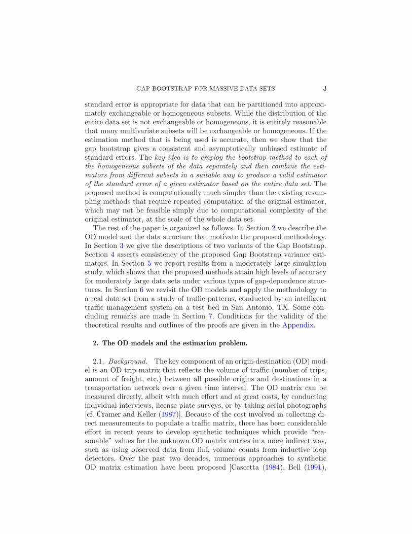
Figures 2 and 3 give the box-plots of the differences between the GapBootstrap I standard error estimates and the true standard errors in theone-dimensional case under centered exponential and under normal errordistributions, respectively. Here box-plots in the top panels are based on theAR(2) model, the middle panels are based on the MA(2) model, while thebottom panels are based on the periodic model. For each model, the combi-nations of (n,p) are given by (n,p) = (200,5), (500,10), (1800,30), (3500,50),(6000,75), (10,000,100).
Similarly, Figures 4 and 5 give the corresponding box-plots for the GapBootstrap II method under centered exponential and under normal errordistributions, respectively.
From the Figures 4 and 5, it is evident that the variability of the standarderror estimates from the Gap Bootstrap I Method is higher under Models Iand II than under Model III for both error distributions. However, the biasunder Model III is persistently higher even for larger values of the samplesize. This can be explained by noting that for Method I, the assumptionof approximate exchangeability of the rows is violated under the periodicmean structure of Model III, leading to a bigger bias. In comparison, Gap
GAP BOOTSTRAP FOR MASSIVE DATA SETS 15
Fig. 2. Box-plots of the differences between the standard error estimates based on GapBootstrap I and the true standard errors in the one-dimensional case using 500 simulationruns. Here, plots in the first panel are based on Model I, those in the second and third panelsare based on Models II and III, respectively. The values of (n,p) for each box-plot are givenat the bottom of the third panel. The innovation distribution is centered exponential.
Bootstrap II estimates tend to center around the target value (i.e., withdifferences around zero) even for the periodic model. Table 1 gives the true
values of the standard errors of θn based on Monte-Carlo simulation and thecorresponding summary measures for Gap Bootstrap methods I and II in 18out of the 36 cases [we report only the first 3 combinations of (n,p) to savespace. A similar pattern was observed in the other 18 cases].
From the table, we make the following observations:
(i) The biases of the Gap Bootstrap I estimators are consistently higherthan those based on Method II under Models I and II for both normaland nonnormal errors, resulting in higher overall MSEs for Gap BootstrapI estimators.
(ii) Unlike under Models I and II, here the biases of the two methodscan have opposite signs.
(iii) From the last column of Table 1 (which gives the ratios of the MSEsof estimators based on Methods I and II), it follows that the Gap BootstrapII works significantly better than Gap Bootstrap I for Models I and II. For

16 LAHIRI, SPIEGELMAN, APPIAH AND RILETT
Fig. 3. Box-plots for the differences of Gap Bootstrap I estimates and the true standarderrors as in Figure 2, but under normal innovation distribution.
Model III, neither method dominates the other in terms of bias and/or MSE.MSE comparison shows a curious behavior of Method I at (n,p) = (500,10)for the periodic model.
(iv) The nonnormality of theXt’s does not seem to have significant effectson the relative accuracy of the two methods.
Next we consider performance of the two gap Bootstrap methods for mul-tivariate data. The models we consider are analogs of (I)–(III) above, withthe general structure
Yt = (0.2,0.3,0.4,0.5)′ +Zt, t≥ 1,
where Zt is taken to be the following: (IV) a multivariate autoregressive(MAR) process, (V) a multivariate moving average (MMA) process, and(VI) a multivariate periodic process. For the MAR process,
Zt =ΨZt−1 + et,
where
Ψ=
0.5 0 0 0
0.1 0.6 0 0
0 0 −0.2 0
0 0.1 0 0.4

GAP BOOTSTRAP FOR MASSIVE DATA SETS 17
Fig. 4. Box-plots of the differences of standard error estimates based on Gap BootstrapII and the true standard errors in the one-dimensional case, as in Figure 2, under thecentered exponential innovation distribution.
and the et are i.i.d. d= 4 dimensional normal random vectors with mean 0and covariance matrix Σ0, where we consider two choices of Σ0:
(i) Σ0 is the identity matrix of order 4;(ii) Σ0 has (i, j)th element given by (−ρ)|i−j|, 1≤ i, j ≤ 4, with ρ= 0.55.
For the MMA model, we take
Zt =Φ1et−1 +Φ2et−2 + et,
where et are as above. The matrix of MA coefficients are given by
Φ1 =
1 0 0 0
∗ 2 0 0
∗ ∗ 2 0
∗ ∗ ∗ 2
and Φ2 =
1
8
1 0 0 0
∗ 1 0 0
∗ ∗ 1 0
∗ ∗ ∗ 1
,
where, in both Φ1 and Φ2, the ∗’s are generated by using a random samplefrom the UNIFORM (0,1) distribution [i.e., random numbers in (0,1)] andare held fixed throughout the simulation. We take Φ1 and Φ2 as lower tri-angular matrices to mimic the structure of the OD model for the real data

18 LAHIRI, SPIEGELMAN, APPIAH AND RILETT
Fig. 5. Box-plots of the differences of standard error estimates based on Gap BootstrapII and the true standard errors in the one-dimensional case, as in Figure 2, under thenormal innovation distribution.
example that will be considered in Section 6 below. Finally, the observationsXt under the periodic model (VI) are generated by stacking the univariatecase with the same p, but with µ changed to the the vector (0.2,0.3,0.4,0.5).The component-wise values of α1 and α2 are kept the same and the εt’s forthe 4 components are now given by the et’s, with the two choices of thecovariance matrix.
The parameter of interest is the mean of component-wise means, that is,
θ = µ= [0.2 + 0.3 + 0.4 + 0.5]/4.
The estimator θn is the mean of the component-wise means of the entire dataset and θ(i) is given by the mean of the component-wise means coming fromthe ith row of n/p-many data vectors, for j = 1, . . . , p. Box-plots of the dif-
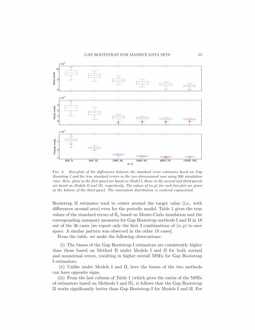
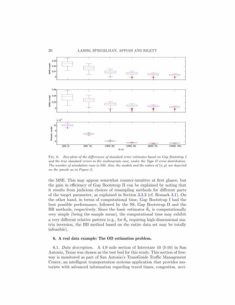
ferences between the true standard errors of θn and their estimates obtainedby the two Gap Bootstrap methods are reported in Figures 6 and 7, respec-tively. We only report the results for the models with covariance structure(ii) above (to save space).
The number of simulation runs is 500 as in the univariate case. From thefigures it follows that the relative patterns of the box-plots mimic those in thecase of the univariate case, with Gap Bootstrap I leading to systematic biases

GAP BOOTSTRAP FOR MASSIVE DATA SETS 19
Table 1Bias and MSEs of Standard Error estimates from Gap Bootstraps I and II for univariate
data for Models I–III. For each model, the two sets of 3 rows correspond to(n,p) = (200,5), (500,10), (1800,30) under the normal (denoted by N in the first column)
and the centered Exponential (denoted by E) error distributions, respectively. HereB-I= Bias of Gap Bootstrap I ×102, M-I=MSE of Gap Bootstrap I ×104, B-II= Biasof Gap Bootstrap II ×103, and M-II=MSE of Gap Bootstrap II ×104. Column 2 givesthe target parameter evaluated by Monte-Carlo simulations and the last column is the
ratio of columns 4 and 6
Model True-se B-I M-I B-II M-II Ratio (fix)
I.N.1 0.013 −0.831 0.708 −0.376 0.029 24.4I.N.2 0.011 −0.700 0.503 −0.118 0.0202 25.2I.N.3 0.008 −0.481 0.241 −0.256 0.0142 17.2
I.E.1 0.065 −4.18 17.8 −1.97 0.623 28.6I.E.2 0.053 −3.54 12.8 −1.52 0.451 28.4I.E.3 0.038 −2.41 6.04 −0.844 0.348 17.4
II.N.1 0.005 −0.240 0.061 −0.178 0.008 7.6II.N.2 0.003 −0.154 0.026 −0.122 0.004 6.5II.N.3 0.002 −0.081 0.007 −0.087 0.001 7.0
II.E.1 0.023 −1.22E 1.59 −1.18 0.183 8.9II.E.2 0.015 −0.767 0.657 −0.288 0.101 6.5II.E.3 0.008 −0.398 0.184 −0.092 0.025 7.4
III.N.1 0.003 −0.125 0.016 −0.183 0.005 3.2III.N.2 0.002 −0.0263 0.0008 −0.065 0.002 0.4III.N.3 0.001 0.059 0.004 −0.028 0.0004 10.0
III.E.1 0.014 −0.619 0.386 −0.549 0.094 4.1III.E.2 0.009 −0.158 0.026 −0.506 0.042 0.6III.E.3 0.005 0.292 0.086 −0.216 0.010 8.6
under the periodic mean structure. For comparison, we have also consideredthe performance of more standard methods, namely, the overlapping versionsof the Subsampling (SS) and the Block Bootstrap (BB).
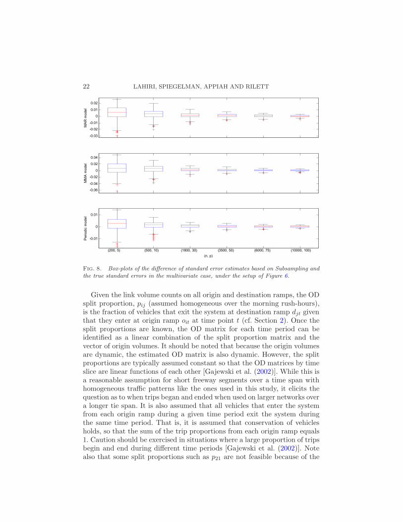
Figures 8 and 9 give box-plots of the differences between the true standarderrors of θn and their estimates obtained by SS and BB methods, underModels (IV)–(VI) with covariance structure (ii). The choice of the block sizewas based on the block length selection rule of Patton, Politis and White(2009). From the figures, it follows that the relative performances of the SSand the BB methods are qualitatively similar and both methods handilyoutperform Gap Bootstrap I.
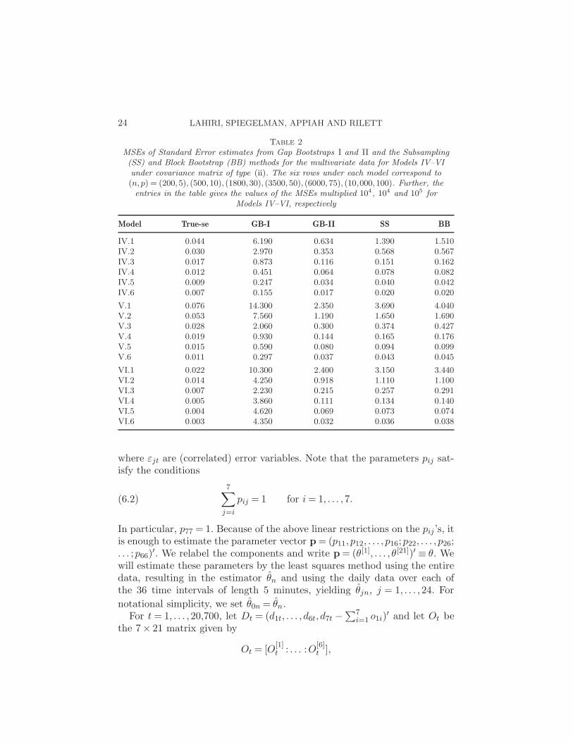
These qualitative observations are more precisely quantified in Table 2which gives the MSEs of all 4 methods for models (IV)–(VI) for all six com-binations of (n,p) under covariance structure (ii). It follows from the tablethat Gap Bootstrap Method II has the best overall performance in terms of
20 LAHIRI, SPIEGELMAN, APPIAH AND RILETT
Fig. 6. Box-plots of the differences of standard error estimates based on Gap Bootstrap Iand the true standard errors in the multivariate case, under the Type II error distribution.The number of simulation runs is 500. Also, the models and the values of (n,p) are depictedon the panels as in Figure 2.
the MSE. This may appear somewhat counter-intuitive at first glance, butthe gain in efficiency of Gap Bootstrap II can be explained by noting thatit results from judicious choices of resampling methods for different partsof the target parameter, as explained in Section 3.3.3 (cf. Remark 3.1). Onthe other hand, in terms of computational time, Gap Bootstrap I had thebest possible performance, followed by the SS, Gap Bootstrap II and theBB methods, respectively. Since the basic estimator θn is computationallyvery simple (being the sample mean), the computational time may exhibit
a very different relative pattern (e.g., for θn requiring high-dimensional ma-trix inversion, the BB method based on the entire data set may be totallyinfeasible).
6. A real data example: The OD estimation problem.
6.1. Data description. A 4.9 mile section of Interstate 10 (I-10) in SanAntonio, Texas was chosen as the test bed for this study. This section of free-way is monitored as part of San Antonio’s TransGuide Traffic ManagementCenter, an intelligent transportation systems application that provides mo-torists with advanced information regarding travel times, congestion, acci-
GAP BOOTSTRAP FOR MASSIVE DATA SETS 21
Fig. 7. Box-plots of the differences of standard error estimates based on Gap BootstrapII and the true standard errors in the multivariate case, under the setup of Figure 6.
dents and other traffic conditions. Archived link volume counts from a seriesof 14 inductive loop detector locations (2 main lane locations, 6 on-rampsand 6 off-ramps) were used in this study (see Figure 1). The analysis is basedon 575 days of peak AM (6:30 to 9:30) traffic count data (All weekdays—January 1, 2007 to March 13, 2009). Each day’s data were summarized into36 volume counts of 5-minute duration. Thus, there were a total of 20,700time points, and each time point giving 14 origin-destination traffic data,resulting in more than a quarter-million data-values. Figures 10 and 11 areplots showing the periodic behavior of the link volume count data at the 7origin (O1 to O7) and 7 destination (D1 to D7) locations, respectively.
6.2. A synthetic OD model. As described in Section 2, the OD trip ma-trix is required in many traffic applications such as traffic simulation mod-els, traffic management, transportation planning and economic development.However, due to the high cost of direct measurements, the OD entries areconstructed using synthetic OD models [Cascetta (1984), Bell (1991), Oku-tani (1987), Dixon and Rilett (2000)]. One common approach for estimatingthe OD matrix from link volume counts is based on the least squares regres-sion where the unknown OD matrix is estimated by minimizing the squaredEuclidean distance between the observed link volumes and the estimatedlink volumes.
22 LAHIRI, SPIEGELMAN, APPIAH AND RILETT
Fig. 8. Box-plots of the difference of standard error estimates based on Subsampling andthe true standard errors in the multivariate case, under the setup of Figure 6.
Given the link volume counts on all origin and destination ramps, the ODsplit proportion, pij (assumed homogeneous over the morning rush-hours),is the fraction of vehicles that exit the system at destination ramp djt giventhat they enter at origin ramp oit at time point t (cf. Section 2). Once thesplit proportions are known, the OD matrix for each time period can beidentified as a linear combination of the split proportion matrix and thevector of origin volumes. It should be noted that because the origin volumesare dynamic, the estimated OD matrix is also dynamic. However, the splitproportions are typically assumed constant so that the OD matrices by timeslice are linear functions of each other [Gajewski et al. (2002)]. While this isa reasonable assumption for short freeway segments over a time span withhomogeneous traffic patterns like the ones used in this study, it elicits thequestion as to when trips began and ended when used on larger networks overa longer tie span. It is also assumed that all vehicles that enter the systemfrom each origin ramp during a given time period exit the system duringthe same time period. That is, it is assumed that conservation of vehiclesholds, so that the sum of the trip proportions from each origin ramp equals1. Caution should be exercised in situations where a large proportion of tripsbegin and end during different time periods [Gajewski et al. (2002)]. Notealso that some split proportions such as p21 are not feasible because of the

GAP BOOTSTRAP FOR MASSIVE DATA SETS 23
Fig. 9. Box-plots of the differences of standard error estimates based on the block boot-strap and the true standard errors in the multivariate case, under the setup of Figure 6.
structure of the network. Moreover, all vehicles that enter the freeway fromorigin ramp 7 go through destination ramp 7 so that p77 = 1. All of theseconstraints need to be incorporated into the estimation process.
Let djt denote the volume at destination j over the tth time interval (ofduration 5 minutes) and ojt denote the jth origin volume over the sameperiod. Let pij be the proportion of origin i volume contributing to thedestination j volume (assumed not to change over time). Then, the syntheticOD model for the link volume counts can be described as follows:
For each t,
d1t = o1tp11 + ε1t,
d2t = o1tp12 + o2tp22 + ε2t,
d3t = o1tp13 + o2tp23 + o3tp33 + ε3t,
d4t = o1tp14 + o2tp24 + o3tp34 + o4tp44 + ε4t,(6.1)
d5t = o1tp15 + o2tp25 + o3tp35 + o4tp45 + o5tp55 + ε5t,
d6t = o1tp16 + o2tp26 + o3tp36 + o4tp46 + o5tp56 + o6tp66 + ε6t,
d7t = o1tp17 + o2tp27 + o3tp37 + o4tp47 + o5tp57 + o6tp67
+ o7tp77 + ε7t,
24 LAHIRI, SPIEGELMAN, APPIAH AND RILETT
Table 2MSEs of Standard Error estimates from Gap Bootstraps I and II and the Subsampling(SS) and Block Bootstrap (BB) methods for the multivariate data for Models IV–VIunder covariance matrix of type (ii). The six rows under each model correspond to(n,p) = (200,5), (500,10), (1800,30), (3500, 50), (6000, 75), (10,000,100). Further, theentries in the table gives the values of the MSEs multiplied 104, 104 and 105 for
Models IV–VI, respectively
Model True-se GB-I GB-II SS BB
IV.1 0.044 6.190 0.634 1.390 1.510IV.2 0.030 2.970 0.353 0.568 0.567IV.3 0.017 0.873 0.116 0.151 0.162IV.4 0.012 0.451 0.064 0.078 0.082IV.5 0.009 0.247 0.034 0.040 0.042IV.6 0.007 0.155 0.017 0.020 0.020
V.1 0.076 14.300 2.350 3.690 4.040V.2 0.053 7.560 1.190 1.650 1.690V.3 0.028 2.060 0.300 0.374 0.427V.4 0.019 0.930 0.144 0.165 0.176V.5 0.015 0.590 0.080 0.094 0.099V.6 0.011 0.297 0.037 0.043 0.045
VI.1 0.022 10.300 2.400 3.150 3.440VI.2 0.014 4.250 0.918 1.110 1.100VI.3 0.007 2.230 0.215 0.257 0.291VI.4 0.005 3.860 0.111 0.134 0.140VI.5 0.004 4.620 0.069 0.073 0.074VI.6 0.003 4.350 0.032 0.036 0.038
where εjt are (correlated) error variables. Note that the parameters pij sat-isfy the conditions
7∑
j=i
pij = 1 for i= 1, . . . ,7.(6.2)
In particular, p77 = 1. Because of the above linear restrictions on the pij ’s, itis enough to estimate the parameter vector p= (p11, p12, . . . , p16;p22, . . . , p26;. . . ;p66)
′. We relabel the components and write p= (θ[1], . . . , θ[21])′ ≡ θ. Wewill estimate these parameters by the least squares method using the entiredata, resulting in the estimator θn and using the daily data over each ofthe 36 time intervals of length 5 minutes, yielding θjn, j = 1, . . . ,24. For
notational simplicity, we set θ0n = θn.For t= 1, . . . ,20,700, let Dt = (d1t, . . . , d6t, d7t −
∑7i=1 o1i)
′ and let Ot bethe 7× 21 matrix given by
Ot = [O[1]t : . . . :O
[6]t ],

GAP BOOTSTRAP FOR MASSIVE DATA SETS 25
Fig. 10. Plots of the origin volume counts for the San Antonio, TX data (includingweekend days).

26 LAHIRI, SPIEGELMAN, APPIAH AND RILETT
Fig. 11. Plots of the destination volume counts for the San Antonio, TX data (includingweekend days).
GAP BOOTSTRAP FOR MASSIVE DATA SETS 27
where, for k = 1, . . . ,6, O[k]t is a 7× (7− k) matrix with its last row given by
(−okt, . . . ,−okt) and the rest of the elements by
(O[k]t )ij = okt1(i≥ k)1(j = i− k+ 1), i= 1, . . . ,6, j = 1, . . . ,7− k.
For j = 0,1, . . . ,36, let
θjn =
[∑
t∈Tj
O′tOt
]−1∑
t∈Tj
O′tDt,(6.3)
where Tj = j, j + 36, . . . , j + (574 × 36) for j = 1, . . . ,36 and where T0 =1, . . . ,720. Note that each of T1, . . . , T36 has size 575 (the total numberof days) and corresponds to the counts data over the respective 5 minuteperiod, while T0 has size 20,700 and it corresponds to the entire data set.For applying Gap Bootstrap II, we need a minor extension of the formulasgiven in Section 3.3, as the weights in (3.4) now vary component-wise. Forj = 0,1, . . . ,36, define Γjn =
∑t∈Tj
O′tOt. Then, the following version of (3.4)
holds [without the op(1) term]:
θn =
36∑
j=1
Wjnθjn,
where Wjn = Γ−10nΓjn. This can be proved by noting that
θn = Γ−10n
∑
t∈T0
O′tDt = Γ−1
0n
36∑
j=1
∑
t∈Tj
O′tDt ≡
36∑
j=1
Wjnθjn.
The Gap Bootstrap II estimator of the variance of the individual components
θ[1]n , . . . , θ
[21]n of the estimator θn is now given by
Var(θ[a]n ) =
36∑
k=1
36∑
l=1
σakσalρa(k, l), a= 1, . . . ,21,
where σ2ak =w′akΣ
(k)wak, Σ(k) is the i.i.d. bootstrap based estimator of the
variance matrix of θkn, ρa(k, j) is the sampling window estimator of thecorrelation between the ath component of the kth and jth row-wise es-timators of θ and wak’s are weights based on Wjn’s. Indeed, with e1 =(1,0, . . . ,0)′, . . . ,e21 = (0, . . . ,1)′, we have waj = e′aΓ
−10nΓjn, 1 ≤ j ≤ 36. To
find ρa(k, j)’s, we applied the sampling window method estimator withℓ= 17 and the following formula for ρa(k, j):
ρa(k, j) =I−1
∑Ii=1(w
′ak[θ
(i)kn − θn])(w
′aj [θ
(i)jn − θn])
[I−1∑I
i=1(w′ak[θ
(i)kn − θn])2]1/2[I−1
∑Ii=1(w
′aj [θ
(i)jn − θn])2]1/2
,

28 LAHIRI, SPIEGELMAN, APPIAH AND RILETT
Table 3Standard Error estimates from Gap Bootstraps I and II (denoted by STD-I
and STD-II, resp.) for the San Antonio, TX data
pij Estimates STD-I STD-II pij Estimates STD-I STD-II
p11 0.355 0.0009 0.0019 p33 0.046 0.0026 0.0041p12 0.104 0.0018 0.0042 p34 0.232 0.0032 0.0132p13 0.011 0.0006 0.0015 p35 0.106 0.0061 0.0082p14 0.064 0.0043 0.0131 p36 0.039 0.0025 0.0080p15 0.047 0.0024 0.0073 p44 0.436 0.0100 0.0155p16 0.022 0.0017 0.0042 p45 0.240 0.0123 0.0094p22 0.385 0.0079 0.0118 p46 0.105 0.0057 0.0141p23 0.083 0.0044 0.0066 p55 0.233 0.0080 0.0130p24 0.242 0.0053 0.0237 p56 0.109 0.0045 0.0168p25 0.112 0.0107 0.0144 p66 0.537 0.0093 0.0263p26 0.064 0.0037 0.0058
j, k = 1, . . . ,36, a= 1, . . . ,21, where θ(i)kn’s is the ith subsample version of θkn
and I = 575− ℓ+ 1 = 559. Following the result on the optimal order of theblock size for estimation of (co)-variances in the block resampling literature[cf. Lahiri (2003)], here we have set ℓ= cN1/3 with N = 575 and c= 2.
Table 3 gives the estimated standard errors of the least squares estimatorsof the 21 parameters θ1, . . . , θ21.
From the table, it is evident that the estimates generated by Gap Boot-strap I are consistently smaller than those produced by Gap Bootstrap II.To verify the presence of serial correlation within columns, we also computedthe component-wise sample autocorrelation functions (ACFs) for each of ori-gin and destination time series (not shown here). From these, we found thatthere is nontrivial correlation in all other series up to lag 14 and that theACFs are of different shapes. In view of the nonstationarity of the compo-nents and the presence of nontrivial serial correlation, it seems reasonable toinfer that Gap Bootstrap I underestimates the standard error of the split pro-portion estimates in the synthetic OD model and, hence, Gap Bootstrap IIestimates may be used for further analysis and decision making.
7. Concluding remarks. In this paper we have presented two resamplingmethods that are suitable for carrying out inference on a class of massivedata sets that have a special structural property. While naive applications ofthe existing resampling methodology are severely constrained by the com-putational issues associated with massive data sets, the proposed methodsexploit the so-called “gap” structure of massive data sets to split them intowell-behaved smaller subsets where judicious combinations of known resam-pling techniques can be employed to obtain subset-wise accurate solutions.Some simple analytical considerations are then used to combine the piece-wise results to solve the original problem that is otherwise intractable. As
GAP BOOTSTRAP FOR MASSIVE DATA SETS 29
is evident from the discussions earlier, the versions of the proposed GapBootstrap methods require different sets of regularity conditions for theirvalidity. Method I requires that the different subsets (in our notation, rows)have approximately the same distribution and that the number of such sub-sets be large. In comparison, Method II allows for nonstationarity amongthe different subsets and does not require the number of subsets itself to goto infinity. However, the price paid for a wider range of validity for MethodII is that it requires some analytical considerations [cf. (3.4)] and that it usesmore complex resampling methodology. We show that the analytical consid-erations are often simple, specifically for asymptotically linear estimators,which cover a number of commonly used classes of estimators. Even in thenonstationary setup, such as in the regression models associated with thereal data example, finding the weights in (3.4) is not very difficult. In themoderate scale simulation of Section 5, Method II typically outperformedall the resampling methods considered here, including, perhaps surprisingly,the block bootstrap on the entire data set; This can be explained by notingthat unlike the block bootstrap method, Method II crucially exploits the gapstructure to estimate different parts by using a suitable resampling methodfor each part separately. On the other hand, Method I gives a “quick andsimple” alternative for massive data sets that has a reasonably good per-formance whenever the data subsets are relatively homogeneous and thenumber of subsets is large.
APPENDIX: PROOFS
For clarity of exposition, we first give a relatively detailed proof of The-orem 4.2 in Section A.1 and then outline a proof of Theorem 4.1 in Sec-tion A.2.
A.1. Proof of consistency of Method II.
A.1.1. Conditions. Let Ytt∈Z be a d-dimensional time series on aprobability space (Ω,F , P ) with strong mixing coefficient
α(n)≡ sup|P (A∩B)−P (A)P (B)| :A ∈ Fa∞,B ∈ F∞
a+n, a ∈ Z, n≥ 1,
where Z = 0,±1,±2, . . . and where Fba = σ〈Yt : t ∈ [a, b] ∩ Z〉 for −∞ ≤
a≤ b≤∞. We suppose that the observations Xt : t= 1, . . . , n are obtainedfrom the Yt-series with systematic deletion of Yt-subseries of length q, asdescribed in Section 2.2, leaving a gap of q in between two columns of X,that is, (X1, . . . ,Xp) = (Y1, . . . ,Yp), (Xp+1, . . . ,X2p = (Yp+q+1, . . . ,Y2p+q),etc. Thus, for i= 0, . . . ,m− 1 and j = 1, . . . , p,
Xip+j =Yi(p+q)+j.
Further, suppose that the vectorized process (Xip+1, . . . ,X(i+1)p) : i≥ 0 isstationary. Thus, the original process Yt is nonstationary, but it has a
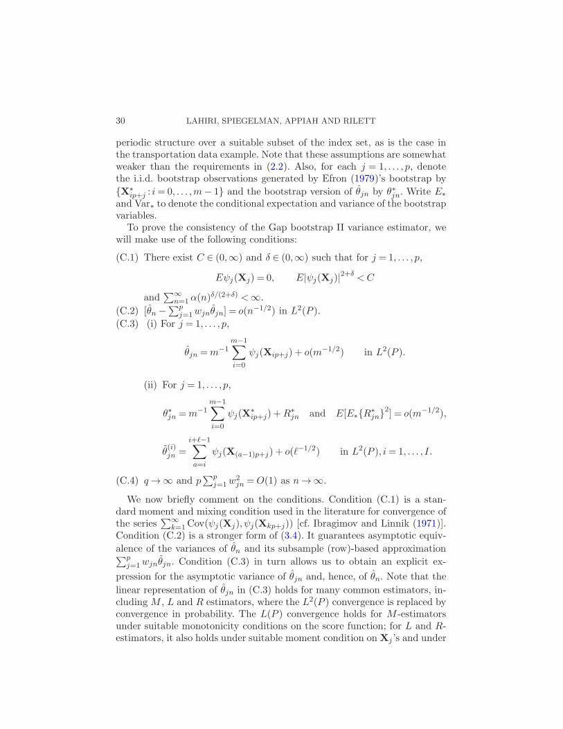
30 LAHIRI, SPIEGELMAN, APPIAH AND RILETT
periodic structure over a suitable subset of the index set, as is the case inthe transportation data example. Note that these assumptions are somewhatweaker than the requirements in (2.2). Also, for each j = 1, . . . , p, denotethe i.i.d. bootstrap observations generated by Efron (1979)’s bootstrap by
X∗ip+j : i= 0, . . . ,m− 1 and the bootstrap version of θjn by θ∗jn. Write E∗
and Var∗ to denote the conditional expectation and variance of the bootstrapvariables.
To prove the consistency of the Gap bootstrap II variance estimator, wewill make use of the following conditions:
(C.1) There exist C ∈ (0,∞) and δ ∈ (0,∞) such that for j = 1, . . . , p,
Eψj(Xj) = 0, E|ψj(Xj)|2+δ <C
and∑∞
n=1α(n)δ/(2+δ) <∞.
(C.2) [θn −∑p
j=1wjnθjn] = o(n−1/2) in L2(P ).
(C.3) (i) For j = 1, . . . , p,
θjn =m−1m−1∑
i=0
ψj(Xip+j) + o(m−1/2) in L2(P ).
(ii) For j = 1, . . . , p,
θ∗jn =m−1m−1∑
i=0
ψj(X∗ip+j) +R∗
jn and E[E∗R∗jn
2] = o(m−1/2),
θ(i)jn =
i+ℓ−1∑
a=i
ψj(X(a−1)p+j) + o(ℓ−1/2) in L2(P ), i= 1, . . . , I.
(C.4) q→∞ and p∑p
j=1w2jn =O(1) as n→∞.
We now briefly comment on the conditions. Condition (C.1) is a stan-dard moment and mixing condition used in the literature for convergence ofthe series
∑∞k=1Cov(ψj(Xj), ψj(Xkp+j)) [cf. Ibragimov and Linnik (1971)].
Condition (C.2) is a stronger form of (3.4). It guarantees asymptotic equiv-
alence of the variances of θn and its subsample (row)-based approximation∑pj=1wjnθjn. Condition (C.3) in turn allows us to obtain an explicit ex-
pression for the asymptotic variance of θjn and, hence, of θn. Note that the
linear representation of θjn in (C.3) holds for many common estimators, in-cludingM , L and R estimators, where the L2(P ) convergence is replaced byconvergence in probability. The L(P ) convergence holds for M -estimatorsunder suitable monotonicity conditions on the score function; for L and R-estimators, it also holds under suitable moment condition on Xj ’s and under

GAP BOOTSTRAP FOR MASSIVE DATA SETS 31
suitable growth conditions on the weight functions. Condition (C.3)(ii) re-quires that a linear representation similar to that of the row-wise estimatorθjn holds for its i.i.d. bootstrap version θ∗jn. If the bootstrap variables X∗
ip+jare defined on (Ω,F , P ) (which can always be done on a possibly enlargedprobability space), then the iterated expectation E[E∗R
∗jn
2] is the same
as the unconditional expectation ER∗jn
2, and the first part of (C.2)(ii) canbe simply stated as
θ∗jn =m−1m−1∑
i=0
ψj(X∗ip+j) + o(m−1/2) in L2(P ).
The second part of (C.2)(ii) is an analog of (C.2)(i) for the subsample ver-
sions of the estimators θjn’s. The remainder term here is o(ℓ−1/2), as thesubsampling estimators are now based on ℓ columns of Xt-variables as op-posed to m columns for θjn’s. All the representations in condition (C.3) holdfor suitable classes of M , L and R estimators, as described above.
Next consider condition (C.4). It requires that the gap between the Yt
variables in two consecutive columns of X go to infinity, at an arbitrary
rate. This condition guarantees that the i.i.d. bootstrap of Efron (1979)
yields consistent variance estimators for the row-wise estimators θjn’s, evenin presence of (weak) serial correlation. The second part of condition (C.4)is equivalent to requiring wjn =O(1) for each j = 1, . . . , p, when p is fixed.For simplicity, in the following we only prove Theorem 4.2 for the case pis fixed. However, in some applications, “p→∞” may be a more realisticassumption and, in this case, Theorem 4.2 remains valid provided the ordersymbols in (C.3) have the rate o(m−1/2) uniformly over j ∈ 1, . . . , p, inaddition to the other conditions.
A.1.2. Proofs. Let θ†n =∑p
j=1wjnθjn and θ†jn = m−1∑m−1
i=0 ψj(Xip+j),
j = 1, . . . , p. Let K denote a generic constant in (0,∞) that does not dependon n. Also, unless otherwise specified, limits in order symbols are taken byletting n→∞.
Proof of Theorem 4.2. First we show that
n
∣∣∣∣∣Var(θn)−p∑
j=1
p∑
k=1
wjnwknCov(θjn, θkn)
∣∣∣∣∣= o(1).(A.1)
Let ∆n = θn− θ†n. Note that by condition (C.2), E∆2n = o(1). Hence, by the
Cauchy–Schwarz inequality, the left side of (A.1) equals
n|E(θn −Eθn)2 −E(θ†n −Eθ†n)
2|
≤ 2n|E(θ†n −Eθ†n)(∆n −E∆n)|+ nVar(∆n)

32 LAHIRI, SPIEGELMAN, APPIAH AND RILETT
≤ 2n[Var(θ†n)]1/2(E∆2
n)1/2 +E∆2
n
= o(1),
provided Var(θ†n) =O(1).
To see that Var(θ†n) =O(1), note that
mVar(θ†jn) =m−1Var
(m−1∑
i=0
ψj(Xip+j)
)
= Eψj(Xj)2 +2m−1
m−1∑
k=1
(m− k)Eψj(Xj)ψj(Xkp+j)(A.2)
= Eψj(Xj)2 + o(1)
as, by conditions (C.1) and (C.4),
2m−1m−1∑
k=1
(m− k)|Eψj(Yj)ψj(Yk(p+q)+j)|
≤K
m−1∑
k=1
α(k[p+ q])δ/(2+δ)(E|ψj(Xj)|2+δ)2/(2+δ)
≤C2/(2+δ)K∞∑
k=p+q
α(k)δ/(2+δ) = o(1).
By similar arguments, for any 1≤ j, k ≤ p,
mCov(θ†jn, θ†kn) =Eψj(Xj)ψk(Xk) + o(1).(A.3)
Also, by (A.2) and conditions (C.3) and (C.4),
nVar(θ†n) = n
p∑
j=1
w2jnVar(θjn) + 2n
∑
1≤j<k≤p
|wjnwkn||Cov(θjn, θkn)|
=O
([p∑
j=1
|wjn|
]2nm−1
)=O(1).
Hence, (A.1) follows.To complete the proof of the theorem, by (A.1), it now remains to show
that
m[σ2jn −Var(θjn)] = op(1),(A.4)
ρn(j, k)− ρn(j, k) = op(1)(A.5)
for all 1 ≤ j, k ≤ p, where ρn(j, k) is the correlation between θjn and θkn.
First consider (A.4). Note that by (A.2), mVar(θjn) =Eψj(Xj)2+ o(1) and

GAP BOOTSTRAP FOR MASSIVE DATA SETS 33
by condition (C.3)(ii),
mσ2jn =mVar∗
(m−1
m−1∑
i=0
ψj(X∗ip+j)
)+ op(1).
By using a truncation argument and the mixing condition (C.4), it is easyto show that
m−1m−1∑
i=0
[ψj(Xip+j)]r =E[ψj(Xip+j)]
r + op(1), r= 1,2.
Hence, (A.4) follows. Next, to prove (A.5), note that by condition (C.3),(A.2) and (A.3),
ρn(j, k) =Eψj(Xj)ψk(Xk)
[Eψj(Xj)2]1/2[Eψk(Xk)2]1/2+ o(1)
for all j, k. Also, by conditions (C.3)–(C.4) and standard variance boundunder the moment and mixing conditions of (C.4), for all j, k,
I−1I∑
i=1
θ(i)jn θ
(i)kn = I−1
I∑
i=1
θ†(i)jn θ
†(i)kn + op(ℓ
−1/2),
where θ†(i)jn =
∑i+ℓ−1a=i ψj(X(a−1)p+j), i= 1, . . . , I . The consistency of the sam-
pling window estimator of ρn(j, k) can now be proved by using conditions(C.2), (C.3) and standard results [cf. Theorem 3.1, Lahiri (2003)]. This com-pletes the proof of (A.5) and hence of Theorem 4.2.
Proofs of (3.9) and (3.10). For notational simplicity, w.l.g., we setµ = 0. (Otherwise, replace Xt by Xt − µ for all t in the following steps.)Write Xjn and X(k), respectively, for the sample averages of the jth rowand kth column, 1≤ j ≤ p and 1≤ k ≤m. First consider (3.9). Since µ= 0,it follows that for each j ∈ 1, . . . , p,
θjn =m−1m∑
i=1
X2(i−1)p+j − X2
jn =m−1m∑
i=1
X2(i−1)p+j +Op(n
−1).
Since n=mp, using a similar argument, it follows that θn = n−1∑n
i=1X2i +
Op(n−1) = p−1
∑pj=1 θjn +Op(n
−1). Hence, (3.9) holds.
Next consider (3.10). It is easy to check that for all k = 1, . . . ,m, θ(k) =p−1
∑pi=1X
2(k−1)p+i − [X(k)]2 and E[X(k)]2 = p−21′Σ1. Hence, with Wk =
[X(k)]2 −E[X(k)]2,
θn = n−1n∑
i=1
X2i +Op(n
−1)

34 LAHIRI, SPIEGELMAN, APPIAH AND RILETT
=m−1m∑
k=1
[θ(k) + X(k)2] +Op(n−1)
=m−1m∑
k=1
θ(k) + p−21′Σ1+m−1m∑
k=1
Wk +Op(n−1)
=m−1m∑
k=1
θ(k) + p−21′Σ1+Op(n−1/2),
provided condition (C.1) holds with ψj(x) = x2 for all j. Further, note
that the leading part of the Op(n−1/2)-term is n−1/2 ×m−1/2
∑mk=1Wk and
m−1/2 ×∑m
k=1Wk is asymptotically normal with mean zero and variance
σ2W ≡ Var(W1) + 2∑∞
i=1Cov(W1,Wi+1). As a result, the Op(n−1/2)-term
cannot be of a smaller order (except in the special case of σ2W = 0).
A.2. Proof of consistency of Method I.
A.2.1. Conditions. We shall continue to use the notation and conven-tions of Section A.1.2. In addition to assuming that X satisfies (2.2), weshall make use of the following conditions:
(A.1) (i) Pairwise distributions of m1/2(θjn− θ) : 1≤ j ≤ p are identical.
(ii) m1/2(θjn − θ) : 1≤ j ≤ p are m0-dependent with m0 = o(p).
(A.2) (i) mVar(θ1n)→Σ and mCov(θ1n, θ2n)→ Λ as n→∞.
(ii) [m1/2(θ1n − θ)]2 :n≥ 1 is uniformly integrable.
(iii) mp−1∑p
j=1 Var(θjn)→p Σ as n→∞.
Now we briefly comment on the conditions. As indicated earlier, for thevalidity of the Gap Bootstrap I method, we do not need the exchangeabilityof the rows of X; the amount of homogeneity of the centered and scaledrow-wise estimators m1/2(θjn − θ) : 1 ≤ j ≤ p, as specified by condition(A.1)(i), is all that is needed. (A.1)(i) also provides the motivation behindthe definition of the variance estimator of the pair-wise differences rightabove (3.3). Condition (A.1)(ii) has two implications. First, it quantifies theapproximate independence condition in (2.2). A suitable strong mixing con-dition can be used instead, as in the proof of Theorem 4.2, but we do notattempt such generalizations to keep the proof short. A second implicationof (A.1)(ii) is that p→∞ as n→∞, that is, the number of subsample esti-
mators θjn’s must be large. In comparison, m0 may or may not go to infinitywith n→∞. Next consider condition (A.2). Condition (A.2)(i) says that therow-wise estimators are root-m consistent and that for any pair j 6= k, thecovariance between m1/2(θjn − θ) and m1/2(θkn − θ) has a common limit,

GAP BOOTSTRAP FOR MASSIVE DATA SETS 35
which is what we are indirectly trying to estimate using mVar(θjn − θkn).Condition (A.2)(ii) is a uniform integrability condition that is implied by
E|m1/2(θ1n − θ2n)|2+δ =O(1) [cf. condition (C.1)] for some δ > 0. Part (iii)
of condition (A.2) says that the i.i.d. bootstrap variance estimator appliedto the (average of the) row-wise estimators be consistent. A proof of this canbe easily constructed using the arguments given in the proof of Theorem 4.2,by requiring some standard regularity conditions on the score functions thatdefine the θjn’s in Section 3.2. We decided to state it as a high level conditionto avoid repetition of similar arguments and to save space.
A.2.2. Proof of Theorem 4.1. In view of condition (A.2)(iii) and (3.3),it is enough to show that
m[Var(θ1n − θ2n)−E(θ1n − θ2n)(θ1n − θ2n)′]→p 0.
Since this is equivalent to showing component-wise consistency, without lossof generality, we may suppose that the θjn’s are one-dimensional.
Define Vjk = m(θjn − θkn)21(|m1/2(θjn − θkn)| > an), Wjk = m(θjn −
θkn)21(|m1/2(θjn − θkn)| ≤ an), for some an ∈ (0,∞) to be specified later.
It is now enough to show that
Q1n ≡ p−2∑
1≤j 6=k≤p
|Vjk −EVjk| →p 0,
Q2n ≡ p−2
∣∣∣∣∑
1≤j 6=k≤p
[Wjk −EWjk]
∣∣∣∣→p 0.
By condition (A.2)(ii), [m1/2(θ1n − θ2n)]2 :n ≥ 1 is also uniformly inte-
grable and, hence,
EQ1n ≤ 2E|m1/2(θ1n − θ2n)21(|m1/2(θ1n − θ2n)|> an) = o(1)
whenever an → ∞ as n → ∞. Next consider Q2n. Define the sets J1 =(j, k) : 1≤ j 6= k ≤ p, Aj,k = (j1, k1) ∈ J1 :min|j− j1|, |k−k1| ≤m0 andBj,k = J1 \Aj,k, (j, k) ∈ J1. Then, for any (j, k) ∈ J1, by the m0-dependencecondition,
Cov(Wjk,Wa,b) = 0 for all (a, b) ∈Bj,k.
Further, note that |Aj,k| ≡ the size of Aj,k is at most 2m0p for all (j, k) ∈ J1.Hence, it follows that
EQ22n ≤ p−4
[ ∑
(j,k)∈J1
Var(Wjk) +∑
(j,k)∈J1
∑
(a,b)6=(j,k)
Cov(Wjk,Wab)
]
≤ p−4
[p2EW 2
12 +∑
(j,k)∈J1
∑
(a,b)∈Aj,k
|Cov(Wjk,Wab)|
]

36 LAHIRI, SPIEGELMAN, APPIAH AND RILETT
≤ p−4[p2a2nE|W12|+ p2 · 2m0p · a2nE|W12|]
=O(p−1m0a2n)
as E|W12| ≤ mE(θ1n − θ2n)2 = O(1). Now choosing an = [p/m0]
1/3 (say),we get Qkn →p 0 for k = 1,2, proving (A.6). This completes the proof ofTheorem 4.1.
Acknowledgments. The authors thank the referees, the Associate Editorand the Editor for a number of constructive suggestions that significantlyimproved an earlier draft of the paper.
REFERENCES
Bell, M. G. H. (1991). The estimation of origin-destination matrices by constrainedgeneralised least squares. Transportation Res. 25B 13–22. MR1093618
Cascetta, E. (1984). Estimation of trip matrices from traffic counts and survey data:A generalized least squares estimator. Transportation Res. 18B 289–299.
Cremer, M. and Keller, H. (1987). A new class of dynamic methods for identificationof origin-destination flows. Transportation Res. 21B 117–132.
Dixon, M. P. and Rilett, L. R. (2000). Real-time origin-destination estimation usingautomatic vehicle identification data. In Proceedings of the 79th Annual Meeting of theTransportation Research Board CD-ROM. Washington, DC.
Efron, B. (1979). Bootstrap methods: Another look at the jackknife. Ann. Statist. 7 1–26.MR0515681
Gajewski, B. J., Rilett, L. R., Dixon, P. M. and Spiegelman, C. H. (2002). Robustestimation of origin-destination matrices. Journal of Transportation and Statistics 537–56.
Hall, P. (1992). The Bootstrap and Edgeworth Expansion. Springer, New York.Hall, P. and Jing, B. (1996). On sample reuse methods for dependent data. J. Roy.
Statist. Soc. Ser. B 58 727–737. MR1410187Ibragimov, I. A. and Linnik, Y. V. (1971). Independent and Stationary Sequences of
Random Variables. Wolters-Noordhoff Publishing, Groningen. MR0322926Koul, H. L. (2002). Weighted Empirical Processes in Dynamic Nonlinear Models. Lecture
Notes in Statistics 166. Springer, New York. MR1911855Koul, H. L. and Mukherjee, K. (1993). Asymptotics of R-, MD- and LAD-estimators
in linear regression models with long range dependent errors. Probab. Theory RelatedFields 95 535–553. MR1217450
Kunsch, H. R. (1989). The jackknife and the bootstrap for general stationary observa-tions. Ann. Statist. 17 1217–1241. MR1015147
Lahiri, S. N. (1999). Theoretical comparisons of block bootstrap methods. Ann. Statist.27 386–404. MR1701117
Lahiri, S. N. (2003). Resampling Methods for Dependent Data. Springer, New York.MR2001447
Mannering, F. L., Washburn, S. S. and Kilareski, W. P. (2009). Principles of High-way Engineering and Traffic Analysis, 4th ed. Wiley, Hoboken, NJ.
Okutani, I. (1987). The Kalman filtering approaches in some transportation and traf-fic problems. In Transportation and Traffic Theory (Cambridge, MA, 1987) 397–416.Elsevier, New York. MR1095119

GAP BOOTSTRAP FOR MASSIVE DATA SETS 37
Patton, A., Politis, D. N. and White, H. (2009). Correction to “Automatic block-length selection for the dependent bootstrap” by D. Politis and H. White. EconometricRev. 28 372–375. MR2532278
Politis, D. N. and Romano, J. P. (1994). Large sample confidence regions based onsubsamples under minimal assumptions. Ann. Statist. 22 2031–2050. MR1329181
Roess, R. P., Prassas, E. S. and McShane, W. R. (2004). Traffic Engineering, 3rd ed.Prentice Hall, Englewood Cliffs, NJ.
Serfling, R. J. (1980). Approximation Theorems of Mathematical Statistics. Wiley, NewYork. MR0595165
Singh, K. (1981). On the asymptotic accuracy of Efron’s bootstrap. Ann. Statist. 9 1187–1195. MR0630102
S. N. LahiriC. SpiegelmanDepartment of StatisticsTexas A&M UniversityCollege Station, Texas 77843USAE-mail: [email protected]
J. AppiahL. RilettNebraska Transportation CenterUniversity of Nebraska-Lincoln262D Whittier Research CenterP.O. Box 880531Lincoln, Nebraska 68588-0531USA