an application of linear programming to decision...
TRANSCRIPT

AN APPLICATION OF LINEAR PROGRAMMING TO DECISION RULES FOR OPERATING ELECTRIC POWER SYSTEMS
By
Emile Snijders
The National Regulatory Research Institute 2130 Neil Avenue
Columbus, Ohio 43210
August 1979
79-36

PREFACE
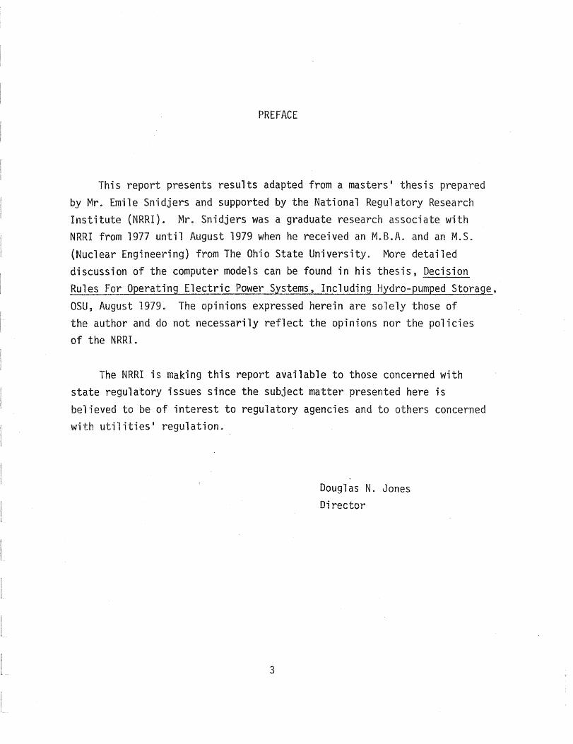
This report presents results adapted from a masters' thesis prepared by Mr. Emile Snidjers and supported by the National Regulatory Research Institute (NRRI). Mr. Snidjers was a graduate research associate with NRRI from 1977 until August 1979 when he received an M.B.A. and an M.S. (Nuclear Engineering) from The Ohio State University. More detailed discussion of the computer models can be found in his thesis, Decision Rules For Operating Electric Power Systems, Including Hydro-pumped Storage, OSU, August 1979. The opinions expressed herein are solely those of the author and do not necessarily reflect the opinions nor the policies of the NRRI.
The NRRI is making this report available to those concerned with state regulatory issues since the subject matter presented here is believed to be of interest to regulatory agencies and to others concerned with utilities' regulation.
Douglas N. Jones Director
3


EXECUTIVE
This report examines optimum ties and hourly generation decision rules through the use of linear programming and chanceconstrained programming. A framework is developed to derive these capacities and generation rules, and they are tested for a specific utility's capacity and load data, name"ly, the Virg"inia Electric Power Company (VEPCO).
The report shows that, if the to optimize capacity, then basic i to generation planning. Therefore, loads, with a certain degree of
load duration curve is used is 1 which is viable
to hour utility , were used to optimize the
system.
The general results of this study~ based on VEPCO information and 1978 cost data, are shown below.
A. Given any 1978 daily 1
( 1 )
(2)
(3)
(4)
pumped storage is cost ye for all days considered in the study; both storage pumping overall reservoir capacities can be satisfactorily explained by maximum and average loads, whereas their load leveling effect makes the capacities of the generati systems depend completely on the average load; in the optimum confi on storage pumping capacity is highly correlated wi overall reservoir capacity; generation is performed in the standard economic loading order, and the storage is filled during the first seven to nine hours and emptied during the peak-load period(s).
B. Given a stochastically determi daily load profile:
(1) pumped storage again is cost-effective for all cases considered;
5

(2) the load uncertainty results in increases in both storage and reservoir capacities corresponding to approximately 2-4 and 3-7 times the size of their deterministic counterparts, for reliability levels ranging from 85 to 99%;
(3) generating costs and capital costs for an optimum system increase non-linearly with the reliability of the system, i.e. the probability of meeting a stochastic demand pattern;
(4) zero-order decision rules can be established with respect to generation scheduling and capacity determination.
c. The linear programming approach for the determination of both capacities and generation levels does yield solutions which can incorporate dynamic aspects of electricity supply (such as plant loading rates, etc.). However, the derived decision rules do need additional adjustments since they were obtained through daily optimizations, which necessarily lead to some suboptimization when these daily time units are aggregated over longer periods.
The recommendations focus on possible future extensions of this ~approach, involving the following aspects:
A. An extension of the model to allow for technical and economic information of individual plants.
B. Extensions to optimize a total yearly period, opposed to the performed daily sub-optimizations.
C. The probabilistic formulation of the hourly loads so that:
(1) the uncertainty related to these loads can be diminished, and
(2) the stochastic decision rules can be improved by accounting for updated information.
D. --The schedul i ng of mai ntenance and unforeseen breakdowns ina longer-term overall optimization framework. In this case a purchased power option is to be included in the system.
6
TABLE OF CONTENTS
EXECUTIVE SUMMARY. LIST OF TABLES . . LIST OF FIGURES .. LIST OF SYMBOLS.
Chapter
1. INTRODUCTION
1.1 Energy Storage and the Utilities 1.2 Research Objectives and Methods .
2. SYSTEM MODELING .....
2.1 2.2
2.3
System Overview. Generating Plants. 2.2.1 Technical Considerations. 2.2.2 Economic Considerations Pumped Storage . . . . . . . . 2.3.1 Description ..... . 2.3.2 Technical Considerations. 2.3.3 Economic Considerations
3. OPTIMIZATION METHODS . .
3.1 Introduction ... 3.2 Linear Programming 3.3 Chance-Constrained Programming
4. MODEL SET-UP ........ .
4.1 4.2 4.3 4.4
4.5
General Description ... The Deterministic Model The Stochastic Model Data Inputs . . . . . . 4.4.1 Loads . . . . . ... 4.4.2 Generating and Pumped Storage Stations. S i mu 1 at ion . . . . . . . . . . . . . . . . . .
7
Page
5 9
10 13
15
15 20
23
23 25 25 27 28 28 31 33
35
35 37 38
39
39 44 49 53 53 58 64

TABLE OF CONTENTS (Continued)
Page
Chapter
5. RESULTS 67
5.1 Deterministic Model ..... ...... 69 5.1.1 Deterministic Models Storage . . . . 69 5.1.2 Deterministic Models With Storage. . 75 5.1.3 Pumped Storage Analysis. . . . . . . . 80
5.2 Stochastic Models . . . . . . . . . . 84 5.2.1 Stochastic Models Excluding ge . 88 5.2.2 Stochastic Models Including Storage. . 88
5.3 S i mu 1 at ion . . . . . . . . . . . . . 100
6. CONCLUSIONS AND RECOMMENDATIONS . 103
104 106
6."1 Conclusions 6.2 Recommendations
REFERENCES
APPENDIX
A. BASIC DATA
A-l Load Data ...... . A-2 Generati ng Stati,on Data A-3 Cost Data
B. SELECTED
B- 1 LPl B-2 LP2 B-3 LP3 Output .
8
107
111
112 113 118
123
124 127 131

LIST OF TABLES
Table Page
4.1 Costs Used in Optimization Models .. 63
5.1 Model Features 68
5.2 Overview of LP1 Results. 70
5.3 Overview of LP2 Results .. 76
5.4 Overview of LPN Results . . 91
5.5 Overview of LPS Results . . 93
5.6 LPS Costs for August With Fixed Capacities at at 99% Reliability. . ................. 96
5.7 LPSV Costs for August for the VEPCa System at 99% Reliability . . . . . . ... · . 95
5.8 Simulation Results . 101
A.l VEPCO Nuclear Unit Specifications . . .. . 114
A.2 VEPCa Coal Unit Specifications . . . . . . 1·15
A.3 VEPCa Oi 1 Unit Specifications · . 116
A.4 Consi Cost timates · . 119
A.5 Cost mates Used in the Study • 121
9

LIST OF FIGURES
Figure
1.1 Overview of Basic Methods Used in this Study
2.1 System Model . . . . . . . . .
2.2 Input-Output, Efficiency and Heat-Rate Curves
2.3 Hydro Pumped Storage System
4.1
4.2
General Linear Programming Set-Up
Computer Models in the Study ....
Page
22
24
26
29
40
42
4.3 Model of Generation and Storage System During Hour t . 46
4.4 Load Da ta Set- Up . . . . . . . .
4.5 Selected Loads for Specific Days in August
4.6 Selected Loads for Types of Days in August
4.7 Selected Loads for Types of Days in January
4.8
4.9
4.10
4.11
5.1
5.2
VEPCO System Heat-Rate Curves
VEPCO System Efficiency Curves .
VEPCO System Input-Output Curves .
Simulation Approach
LPl Generation Results for 8/4 ...
LP1 Generation Results for 10/7 III • \.., •
54
55
56
57
59
60
61
65
71
72
5.3 LP1V Generation Results for 8/4 74
5.4 LP2 Generation Results and Storage Schedules for 8/4 . 77
5.5 LP2 Generation Results and Storage Schedules for 1/1 . . . 78
5.6 LP2V Generation Results and Storage Schedules for 8/4 . . . . . . . . . . . . . . . . . . .
81
10

LIST OF
Figure
5.7 Optimum Storage versus ervoir
5.8 Total Daily System Cost versus
5.9 Optimum System Cost versus 11
5.10 VEPCa Optimum System Cost versus
5.11 Optimum Reservoir Size versus i 1 .;; Ii
5.12 LPN Generation Results for 8/T at a 95% Reliability Level ........ .
5.13 LPN Generation Results for Reliab"i1ity Level ...
5.14 LPNV Generation Results Reliability Level ...
5. 15 LPS Generation Results for 81T Reliability Level .
5.16 LPSV Generation Results for Reliability Level .
a
at a
a
5.17 LPSV Generation Results for 8/l at a Reliability Level
11
99%
Level
. . .
.
.
Page
82
83
85
86
87
89
90
92
97
98
99


Symbol
AMAX
s
C
CA
CAP
CAPMAX
CC
CP
o
IT
OCR
e
GEFF
I
L
LR
N
NSF
PEFF
LIST OF SYMBOLS
Definition
max"imum fraction
column vector of probability
index denoting a systemls component
zero-order sion on generation, 1000 MW
zero-order decision on capacity, 1000 MW
capacity, 1000 MW
maximum capaci ty, 1000 ~'1l"1
daily capacity cost, 1000 MW
fuel cost,
system load, 1000 MW
average system load, 1000 MW
discharging ratio
efficiency~ %
efficiency of storage in generating mode, fraction
input, MMBTU
loading rate, 1000 MW/hour
normally distributed random variable
net storage flow, 1000 MW
efficiency of storage in pumping mode, fraction
13

LIST OF SYMBOLS (Continued)
Symbol Definition
SO standard deviation, 1000 MW
STOREF storage efficiency
t hourly time index
TC total cost, $
X generation, 1000 MW
Z value of normal variable
14

CHAPTER 1
INTRODUCTION
This research was undertaken to gain a better understanding of
the relationships governing generating capacities and power generation~
By using a "simple ll linear programming approach, a framework is developed
which can be of timely interest to regulatory agencies and to others
concerned with utilities' regulation.
Although the report focuses heavily on energy storage, one gains
insight into the large uncertainties which are associated with both
long and short-term utility planning. It is this increased understand
ing which should be of interest to those involved with utilities l
regulation.
Energy Storage and the Utilities
Utilities are required by law to supply power on demand, matching
the output of their generators to the aggregate demands of their cus-
tomers. The Public Utility Regulatory Policies Act of 1978 [29J,
commonly known as IIPURPA,II establishes as one of its purposes I1the
optimization of the efficiency of use of facilities and resources by
electric utilities. 11 One of its provisions requires the state regula
tory authority or nonregulated utilities to determine a cost-effective
load management technique. This method is defined as cost-effective if:
15

"(1) such technique is likely to reduce maximum kilowatt demand on the
electric utility, or (2) the long-run cost-savings to the utility of
such reduction are likely to exceed the long-run costs to the utility
associated with implementation of such technique. II
Several such techniques have been investigated. Among them are
various energy storage methods for load leveling, and methods to reduce
peak loads through selective pricing [4,6, 8, llJ. Each technique,
however, depends largely on the specifics of the situation. This report
focuses on the historically proven method of pumped hydro storage [8]
to level the utility's load. Examination of the daily/weekly variation
of electricity demand shows that there is a steady component which is
present throughout the day/week and a highly variable component which
is affected by daily changes in load, statistical changes in weather,
the specific day of the week, and the price of electricity to the
consumer [6,21, 30J. These daily, weekly and seasonal load variations
on utility systems result in a typical annual system load factor
ranging between 40 and 80% [lJ.
Utilities purchase generating capacity to meet annual peak load
requirements with a specific degree of reliability. Because of the
marked variations in the daily load profile, a portion of the generation
capacity has the capability of generating additional power at low-load
periods; this is the least expensive energy available in the utility
system. Availability of this low-cost, off-peak energy makes the
concept of storage attractive and economi ca lly feas i b 1 e [27 J. The
amount of energy which can be effectively stored on a particular
16

electric ill tern on
load cs, amount
its energy storage 1 i es.
The ts
improved su y J.
"limited
( 1 ) nt in ant
(2) Product; on cost
(3) Use as spi ng reserve
(4) reli ~I i
(5) More cient
In the short run, the
of the capacity factor
ference almost 15
actual utilization of nuclear
Nuclear Division s t
lack 1
creased average 5
were e today US].
As early as the 1 IS,
in managing energy, but it is
between peaking fuels and
has been i fied as a major
ability shi consumption
ute
fuels to more lower
7
tall
i
was
ncl the utilities
se-l generation and
are a result of
-i nel , but may not
ld be an improvement
y, there is a dif
lity and the
i es by EPRI I s
d fference is due to
factors could be in-
if scient energy storage
as a valuable tool
differential
, that energy storage
utility 'industry. The
ive or more scarce fossil
nuclear fuels is

the primary economic force propelling the development of storage tech
nology.
Energy storage in combination with coal and nuclear power plants
will be able to supply a significant part of future peaking and cycling
energy requirements. This will permit the displacement of oil-fired
generating capacity and the substitution of coal or nuclear derived
energy for oil. As other technologies develop, coal and nuclear energy
may be displaced gradually by resources such as solar and fusion; stor
age will prove to be self-modernizing as this technique can readily
utilize energy derived from any source.
Energy storage devices and systems can effectively contribute to
a power system1s spinning reserve. One impact of this use would be the
increased power system efficiency. Spinning reserve is presently pro
vided by running gas turbines and by operating some power plants at
5-10% below their rated capacity which results in reduced efficiency.
If energy storage can recoup this efficiency, then significant savings
can be achievedo
Energy storage systems are likely to have a higher reliability
than conventional generating devices [22J. If this proves to be true,
then power systems which have significant amounts of energy storage
available could get by with a lower reserve margin and still maintain
the required security of supply. A reduction in reserve margin trans
lates into a capital cost credit for the energy storage system.
18

Load lowing by means ene storage would the need
for cycling individual power pl Power plants would still cycle,
but more slowly. The resultant lowering of thermal stress would almost
certai y increase reli 1i reduce maintenance costs. This use
11 no become much more i as 01 cycling ants are
being phased out and
ment.
th more ghly stressed, modern equip-
In our optimism for energy storage, it is important to recognize
that the value and potential benefi i can ved from energy
storage requires the availability low cost energy periods of low
demand. Energy storage is not an energy source, rather it is part of a
strategy for managing energy supply_ For energy to be success
ful, utilities must continue to build and operate baseload coal and
nuclear generating stations today. In future years, conven-
tional sources may be replaced by solar or fusion but for today,
and the immediate future, reliance must be placed on energy
resources which are currently available.
19

The objectives of this study have been to determine:
(1) the optimum capacities of the nuclear, coal and oil-fired
generating systems and of the pumped storage system -- in terms
of reservoir and pumping capacity, -- and
(2) hourly generation decision rules for each system~ yielding minimum
operating and investment costs as well as a high reliability of
supply.
A framework was developed to derive these capacitie~ and generation
rules, as well as to test them for a specific utility's capacity and
load data (The Virginia Electric Power Company [15]).
Two distinct approaches can be used to optimize both capacity and
generation. One method focuses on the yearly load duration curve D,
9, 31, 32J. In using this load duration curve some basic information
is lost since it represents the aggregated load profiles for one year.
Although some progress has been made in incorporating some basic infor
mation in the load duration curve -- such as probabilistic effects
[30J -- it still does not, and cannot contain the dynamics of hourly
load changing effects for each day. Since energy storage is largely
dependent on these specific hour to hour load changes, a direct
approach has to be used which does represent the actual load situation
[3, 13J.
20

nce this on
was made between the computational
365 periods of 24 hours
day during the year. In this
1
i
s i i on a trade-off
sian of opt i mi n9
zation based on the peak
t the utility must
meet is peak load, and that ases are excluded.
gure 1.1 shows an overview objectives of
this study were met. A set of basic and operating information
is used to optimize the generation patterns and ities for a typical
electric power generation system, as
For the optimization n on were used.
The first uses a linear programmi method in which
loads, technological factors) are known with campl
11 inputs (costs,
certa i nty. Due
to the uncertainty in the demand for ectrici a method was
The latter developed which uses chance
derives zero-order sian rules,
capacities. Storage flows become
dep~nding ~emand. A simul
performed th decision es
over time-spans longer than a day.
i
1 i nea r
y ion and for
zed decision functions,
on 1i operations is
gate their reliability
Chapter 2 introduces the system as modelled in the study, whereas
Chapters 3 and 4 describe and develop mathemati approach used in
this study. Chapter 5 then shows some the study results, with the
general conclusions and recommendations listed in Chapter 6.
21

Basic Information
Generation Capacity Economics Loads
I No Pumpe
I Optim
Subopt Mod
I Pumped S
d Storage
izing/ imizing ules
torage
Generation/ Capacity
Information
Compare
~
Generation/ ~ Capaci ty ~--
Information
lit
Simulation
Figure 1.1 Overview of Basic Methods Used in this Study
22

CHAPTER 2
SYSTEM ING
This chapter introduces the system as modeled in this study, as
well as technical and economic i
stations and pumped storage.
System Overview
on on electricity generating
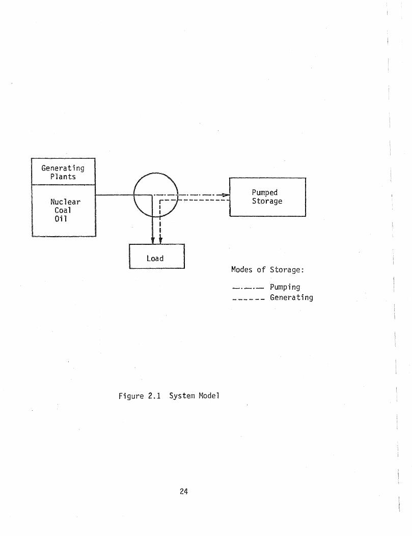
Figure 2.1 shows the system model. The utility's load is supplied
by the generating plants, and by the pumped storage plant if this unit
is in the generating mode. If the latter is in the pumping mode, then
some of the generated power to be determined by an optimization pro-
cedure--is stored for later use.
The components of system, however, have their own technological
and cost characteristics. In order to optimize the design and operations
of the total system it ;s necessary include all the relevant con-
straints and costs for each part the system.
23
Generating Plants
Nuclear Coal Oil
load
Figure 2.1 System Model
24
Pumped Storage
Modes of Storage:
Pumping Generating

General Plants
Technical Considerations
Station performance is most
curves derived from tes on illdi
s y deter'mi by input-output
Figure 2.2a shows
the general trend of this curve, which follows the general p6lynomial
form 2 I = a + bL + cL + ... + (2-1)
where
I = fuel input in MBtu's,
L = output in MWh.
From the basic input-output curve more familiar efficiency curve
(Figure 2.2b) and the heat-rate curve ( 2. ) may be deri ved [26].
The efficiency (e) curve is derived from the formula
e = 3·i13L x 100 percent
and the heat-rate (HR) curve from formula
HR =: J- (in Btu'S!. ) L '\ KHh
(2-2)
(2-3)
From a systems modeling viewpoint, these curves contain all necessary
information for evaluating differences among nuclear, coal and oil-fired
generating stations at a constant power output.
Several differences do, however, exist from a dynamic standpoint.
The loading rate (LR) expresses the rate by which the power output (P)
of a station can be increased, or
_ dP LR - dt • (2-4)

....., N :::3 (j) c..
C I--f
Input-Output Curve
/
Output
(a)
~ 0 c OJ
....... U
"r-"-"-w
1/
Efficiency Curve
Output
(b)
(lJ .J-)
ca a:::
I +-l ca OJ :c
Heat-Rate Curve
Output
(c)
Figure 2.2 Input-Output, Efficiency and Heat-Rate Curves

Thermodynamic considerations
also place upper and lower bounds on
t these loading rates. (They
power output). A constant
loading rate ;s often assumed sufficient for calculations involving
slight power changes [7, J.
Economic Considerations
The relevant costs s ons comprise [17, 20J:
1. Fixed Costs, including
a. Capital Costs (annua"li
b. Fixed Operating and Mai Expenses
2. Variable Costs, includi
a. Fuel Costs
b. Variable Operating Costs
27

Pumped Storage
Deser; pti'on
Hydro pumped storage is distinguished from all other energy storage
methods suitable for utility application in that it has already reached
a mature state of development. Plants have been built and their costs
and characteristics are known. The use of pumped storage in the United
States has, however, been limited. More storage could now be used to
advantage,and expected future loads, generation mixes and fuel costs
point to an expanded role for several possible energy storage methods.
In a hydro pumped storage system, energy is stored by pumping
water from a lower to a higher elevation. The energy is recovered for
utility use by passing the water from the higher to the lower elevation
through a hydro turbine driving an electric generator. Pumping and
generation is accomplished by a reversible pump/turbine connected to a
generator/motor, shown schematically in Figure 2.3. It was the
introduction of this reversible unit, coupled with changing economic
conditions, that contributed substantially to the accelerated interest
and development of pumped storage since the 1960 1 s.
The reservoirs of existing hydro plants or of water storgae systems
can be specially constructed surface reservoirs, underground caverns, or
combinations of these. The pumping-generating plant is connected to the
two reservoirs by appropriate waterways. The power house itself may be
either on the surface or underground -- underground construction has
sometimes been found economically and environmentally desirable, even
where the reservoirs are on the surface [8].
28

Upper Reservoir
Lower Reservoi·r
Figure 2.3 Hydro Pumped Storage System
29
Power In Power Out

Most of the pumped storage capacity now in service can be classi
fied as "pure" pumped storage, i.e, units built only for the storage
of off-peak energy [5J. However, several constructed plants have
additional purposes, including the development of conventional hydro
electric output from natural flow into the upper storage reservoir,
and storage for irregation. In fact, wherever there is a need to
either move or store water, there may be an economic incentive to
develop this into a hydro pumped storaqe system.
The necessity of storing relat"ive"ly large volumes of water in two
reservoirs, separated by several hundred feet of head, requires a
topography that is not available everywhere. Consequently, the
developed and planned pumped storage systems are confined to certain
sections of the country [lJ. rthas, however, been estimated that above
ground pumped storage could be built, if needed and economically
justified, to serve the peaking requirements of the systems which supply
about 70% of the. total electrt.c load in the United States [2].
30

Technical Considerations
Size and Head:
The unit size suitable for utility application will generally be
larger than 200 MW. Smaller units have been built, mostly for specific
applications. Plant size can be any multiple of unit size, although
total plant size is frequently limited by the available reservoir
capacity; and if this is not the limitation, it will usually be the
size that fits the utility system needs.
The heads that have been found economical, in the absence of
special conditions, have been above 300 feet. There are indications
that heads of up to 2500 feet are feasible for single stage reversible
units. For still higher heads, it will be necessary to consider multi
stage units, units in series, or separate pumps and turbines. During
pumping, the lower reservoir is emptied and the upper one is filled; the
gross head is increased. This results in a change of input, but
generally there is a small decrease in pumping.load as the head in
creases.
Efficiency:
Demonstrated over-all efficiencies have been increased from 66% to
75% [8]. These higher efficiencies have been the result of improve
ments in pump/turbine design and of a more liberal design of water
passages. Because over-all efficiency is the product of the separate
pump, motor, generator, transformer (used twice), turbine and waterway
31

(used twice) efficiencies, and because each efficiency is close to its
practical limit, the maximum theoretical efficiency is approximately
80%.
Charge/Discharge Ratio:
The charge/discharge ratio is measured by the relation of power
input (average pumping load in MW) to power output (rated capacity in
MW). Most constructed plants have ratios in the range of 1.0 to 1.3.
The importance of this ratio is its effect on available generating
time. For example, if the ratio is 1.15 and the overall efficiency is
80%, then the duration of generation available from 1 hour of pumping
will be 0.92 hours (= 1.15 * 0.80). These ratios are within the
control of the plant designer with higher ratios obtainable at higher
cost.
Reliability and Availability:
An average availability of about 90% can be established for pumped
hydro systems. (Based on limited historical experience; yielding a
forced outage rate of 4%, and a total 5 weeks of ,ma.intenance per year.)
Turn-Around Ttme and Load Regulating Ability:
A pumped storage plant cannot switch instantaneously from the
pumping mode to the generating mode. A definite time interval is
required due to mechanical and hydraulic inertias. However, 15 minute
time intervals are feasible for each unit in the system.
32

Load following can be accomplished to a limited extent, but
generally its effect on efficiency and on maintenance requirements will
be considered prohibitive in the case of fast load transients.
Economic Considerations
Useful Life:
Hydro units and plants are inherently long-lived property_
Although pumped storage plants are subject to more severe service re
quirements than conventional hydro units because of reversals in the
waterflow direction, maintenance and design do take this into
account, making their life comparable to regular hydro units. For
tax-accounting purposes the Internal Revenue Service allows a life of
50 years for all hydro property.
Costs:
Reservoir capital costs (in $/MWh) and pumping plant costs (in
$/MW) have to be considered separately in an economic analysis. Other
fixed costs include minimal operation and maintenance expenses and
negligable costs such as license fees payable to the Federal Power
Commission, now FERC. Variable costs are virtually nonexistent, due to
the low variable operations and maintenance costs and the absence of
fuel costs.
33


Introduction
CHAPTER 3
OPTIMIZATION METHODS
There are several optimization techniques that can be applied to
the problem of scheduling hourly generation loads and determining over
all capacities simultaneously. Available optimization techniques
include linear, integers dynamics and nonlinear programming.
Of these techniques s classical calculus methods are of limited
use due to the large number of variables involved. However, dynamic,
non-linear, and integer programming are possible alternatives to the
standard linear programming technique.
Direct or exhaustive search is an optimization method which
enumerates all the possible combinations of variables [19]. After
completion of all the enumerations, the selection of the optimal
combination of decision variables is possible. A major disadvantage
is the number of enumerations that must be done.
Dynamic programming is an optimization technique which can markedly
decrease the computational requirements of a large system optimization
[18, 19 s 31, 32]. The reduction in computation is achieved by trans
forming a sequential decision process with interrelated variables into
a series of single-state decision processes involving only a few
35

variables. This means the stages must be decoupled from each other and
that no past decisions affect future decisions and v·ice versa. However,
future decisions can affect the optimality of past decisions because
of the coupling of stages. nee the storage system, especially the
reservoir, depends on past and future information it is not possible
to decouple the stages.
Non-linear programming can handle various types of objective
functions. Some development of algorithms dealing v/ith quadratic
objective functions has been done, but the development of non-linear
algorithms has been limited to a few special appli ions. This
technique is of very limited value because of the large number of
steps required to reach an optimum solution, which consequently
increases the computational time tremendously.
36

Linear Programming
Linear programming is a standard, well-known, technique which has
been used extensively in optimization problems [3, 13, 16, 25J. The
standard formulation is described as:
Maximize Z = ex,
Subject to Ax ~ b,
x 2. 0,
where:
Z is the objective function,
Ax < b are the constraints,
c is a row vector with n elements,
x is a column vector with n elements,
A is a mxn matrix, and
b is a column vector of size m.
(3-1)
(3-2)
(3-3)
The problem is solved by means of the "simplex" method, which (through
an iterative procedure) finds the value of the x vector producing the
optimum in the objective function (Z). The major drawback of this
approach is of course that all the parameters (c, A~ b) have to be known
with certainty. Obviously any random parameter, such as the load on an
electr'icity generating system, does present problems for this approach.
Several methods of mathematical programming have consequently been
developed to account for these problems. The method most applicable
to probabilistic parameters is known as chance-constrained programming
and will be described in the following section.
37

Chanc€-Constra'ined Pro9rammi ng
The standard formulation of chance-constrained programming may be
described as [16, 20]:
Maximize f(cx)
Subject to P(Ax ~ b) ~ a
wher'e P denotes IIprobability,1I and c and A are a non-random vector
(3-4)
(3-5)
and matrix. The vector a contains a set of constants that are proba
bility measures of the extent to which constraint violations are
permitted. Assuming a normally distributed random variable b, with
mean ~ and variance a2 , it is possible to transform the probabilistic
constraint into a deterministic equivalent. Defining by F(z) the
probability that a standardized normal variable will take on a value
between 0 and z, i.e.:
F(z) ::: _1_ jZ ~o
(3-6 )
then each of the equations in the probabilistic constraint set (3-5) can
be stated as
(3-7)
Once all constraints have been transformed in this fashion, it is
possible to solve the model for a given exogenous vector of risks
a ::: (aI' ... , am) and to derive the associated optimum value of the
decision variable vector x ::: (xl' ... , xm). If the values of the xi's
are determined before observing the values of the random variables, then
zero-order decision rules have been established [16, 24J.
38

CHAPTER 4
MODEL SET-UP
This chapter will describe (a) the general set-up of the optimiza
tion models in this study, (b) the deterministic and stochastic
approaches, (c) an overview of the required input data, and (d) the
simulation model, designed to evaluate the derived stochastic decision
rules.
General Description
The general linear programming set-up (see equations 3-1 through
3-3, and Figure 4.1) can be specified to include the following func
tional groups:
Minimize TC = (Fuel Cost for each System) (Fuel Use)
+ (Capacity Cost) (Installed Capacity) (4-1)
Subject to the following constraints;
a) Unit Hourly Power Output of Generating Systems and Storage
2 Unit Capacity of Each System (4-2)
b) Unit Loading Rates < Maximum Unit Loading Rates (4-3)
c) Storage Hourly Outflows ~ Available Energy in Reservoir (4-~·)
d) Available Energy in Reservoir ~ Reservoir Capacity
and
Available Energy in Reservoir> 0
39
(4-6)

Power Output Constraints
Capacity Cost Information
Capacity Constraints
Load Information
CAPACITIES GENERATION LEVELS
Storage Constraints
Fuel Cost Information
Loading Constraints
Figure 4.1 General Linear Programming Set .. Up
40

and finally,
e) Total Hourly Generation + Net Hourly Storage Flow + Required
Power Purchases = Hourly Load (4-7)
The unknowns in this model -7 i.e., the hourly outputs from the nuclear,
coal and oil generation systems, the hourly inflows and outflows to and
from the pumped storage, and the capacities of the generating systems
of the reversible storage turbine/pump and of the storage reservoir
--will be determined by the simplex method. It is essential to include
external power purchases if circumstances such as unforeseen equipment
breakdowns and scheduled maintenance outages are included in the model.
The present approach deals with specific days during which full power
availability is assumed. The resulting minimum cost scenario of capa
cities and hourly generations is sufficient to exclude the purchased
power option.
This study.contains eight different analyses. Based on 1978 load
data, provided by the Virginia Electric Power CompanY9 a deter
ministic model was built. This model was run for all VEPCQ's daily
load profiles in 1978. Figure 4.2 shows the different cases that were
considered for this deterministic approach; namely:
a) Pumped storage excluded, and no upper limits on the capacities
of the generating systems (yielding model LP1)
b) Same as a) but with VEPCQi s total plant capacities (model LP1V)
c) Pumped storage included, and no upper limits on the capacities
of the system's.components (model LP2)
d) Same as c) but with VEPCQ's total plant capacities (model LP2V)
41

Pumped Storage Excluded I Pumped Storage Included --- --r- -- __ .....L_ -- _.- .- -- ---
No Capac; ty I v· .. El t· d PC. i No Capaci ty Constraints I lrglnla ec rlC an ower ompany I Constraints ---~-------~------~-----
I I I I I I I I I I I
I : I
LPl LPIV LP2V LP2
~~---~r __ L_p_NV __ ~~~~ __ LP_S_V __ ~-~~~_L_P_S __ ~
Figure 4.2 Computer Models in the Study
42

For each of these cases the month and type of day was selected which
resulted in the maximum cost scenario for the system. In the LP2V
model the storage and reservoir capacities of this worst case were
lIinstalled" in the system and their financial repercussions investigated
for different load profiles. In LP2 model 1 capacities were again
determined by the maximum cost day. The detrimental effects of dif
ferent generating system mixes again was considered.
Four stochastic models (LPS, LPSV, LPNV, LPN) were built analogous
to the previous approach. Since the uncertainty of the loads in these
models introduces the additional dimension of reliability, this approach
was only investigated for the peak month Again, the capacities for the
maximum cost days were considered binding and their effects were
checked for the other days of the peak month. The resulting generation
decision rules and these above capacities were used in a simulation to
provide a basis "for determining the long-term effects of this sub-opti
mization. In the computer programs, each model builds the required
vectors and matrices. These programs are then linked to the optimiza-
tion code ilLINPRO" which was developed by Dr. Clarence H. Martin, De
partment of Industrial and Systems Engineering, The Ohio State University.
The programs are not listed in this paper since they are assumed II standard ll•
43

TheOetermin1' s-ti c t·1odel
In order to mathematically formulate the optimization model we will
first describe the symbols that will be used. The following sub and
superscripts are defined:
t = time index for hourly intervals (1 through 24)
s = index denoting a system~s component, i.e.,
s = 1 : nuclear
S = 2: coal
S = 3: 011
13 = 4: storage input
S = 5: storage output
The model contains the following unknowns:
X~ = power output of system part 13 during hour t
CApS = capacity of system part 13, where
13 = 1 ~ 3: as before
s = 4: storage pumptng capactty
S = 5: reservoir capacity
The cost vector, c, contains the following elements:
CPs = fuel cost in $/1000 MWh for system part S
CC S = daily capacity cost in $/1000 MW for part S
Other constants included are defined as:
AMAXS = maximum output for system part S as a fraction of 100%
capacity (set equal to 1 in this study).
STOREF = storage efficiency
OCR = discharging ratio
44

PEFF = overall pumping efficiency of storage system
GEFF = overall generating efficiency of storage system
Dt = system load in 1000 MW during hour t, adjusted for
loads continuously supplied by sources not considered
in this analysis
CAPMAXS = maximum capacity considered for system part S
Figure 4.3 shows the set-up of the generation and storage system. Note
that the losses in the storage system, related to its efficiency and its
charge/discharge ratio, were assumed evenly distributed over the pumping
and the generation mode, i.e.,
PEFF = YsTOREF * OCR (4-8)
= overall pumping efficiency, and
GEFF = ~STOREF * OCR (4-9)
::: overall generating efficiency
Chapter 2, Figure 2.2a, presented the input-output curve for generating
stations. It is shown later that it is realistic to assume a linear
curve for which power output is a linear function of fuel input.
The Model is now set up as~
Minimize
Subject to:
1. Maximum capacity constraints
XS - AMAX* CApS < 0 t S -
and,
45
v f t ::: 1 -+ 24
lS:::1-+4
(4-10)

"- X4 * PEFF " \
LOSSES CAp 5
Xl CApl t
CAp2 X2 X5 * GEFF X5
t t /
f
X3 LOSSES
CAp3 t Dt
Figure 4.3 Model of Generation and Storage System During Hour t
46

V t == 1 -+ 24 (4-11) . ~ 2. Storage outflows
(4-12)
T=t-l XS _ ~ (X 5 * PEFF - X4) < 0
t T==l T T -V t == 2 -+ 24 (4-13)
3. Reservoir constraints
¥ t == 1 -+ 24 (4-14)
and,
T==t 4 X 5 * PEFF) < 0 ~ ( - V. t == 1 -+ 24 (4-15) T=l
T -
4. Demand constraints
/13-3 \ \ sL x~ r xi * GEFF - xi == Dt V t == 1 -+ 24 (4-16)
5. Capacity constraints
CApS < CAPMAXS V 13 == 1 -+ 5 (4-17)
4,7

The previous set-up contains 5 * 24 = 120 on variables and 5
capacity variables, thus a total of 125 un as 1 as 221 con-
straint equations. The computer algori culate inverses
of matrices of approximately 150 by 230 elements. It is easily seen
that any extension of this basic model re res care since in-
creasing the size of the matrix to be inverted increases the
computational time -- especially because several te ons are
required. The resulting deterministic model is labeled LP2 or LP2V,
depending upon the specific data input.
The loading rate constraints as in equation (4-3) were
a priori deleted from the model as a result these computational
problems. The justification for droppi constraints is the
assumption that economic load leveling will occur wherever possible (an
inherent characteristic of linear ) . 1 tests have,
however, been performed in which loading rates constraints for selected
periods were included. The results have
direction are feasible. - --
extensions in this
If hydro pumped storage is not to be cons dered, then simply
constraints 2 and 3 (equations 4-12 through 4-15) are dropped, as
well as the unknowns x~ (V t = 1 + 24, 6 = 4 + 5) and CApS (6 = 4 + 5).
The result is model LPI or LP1V, depending on or not the
capacities of the Virginia Electric and Power Company are considered
binding.
48

The Stochastic Model
To account for the statistical variations in the load of the
system a chance-constrained programming approach is introduced. We
will assume that the hourly system load is a normally distributed
variable with mean Dt and standard deviation SOt. Zero-order decision
rules are established as:
XS = CS [t = 1 -+ 24
t t V S = 1 -+ 3
(4-18)
CApS = CAS V S = 1 -+ 5 (4-19)
Note that the storage inflows and outflows have been dropped from the
model; they are intrinsically determined. For convenience sake we will
define a net storage flow during time t (NSFt ) as:
NSF t = Storage Inflows t - Storage Outflows t , or,
(S=3 )
NSFt = I . c~ - 0t S=l
V t = 1 -+ 24 (4-20)
In this approach losses in the storage system h~ve to be neglected
because they have different effects on storage inflows and outflows
whereas it is a priori unknown whether NSFt represents either. A pos
sible solution to this drawback is to select periods in which only
inflows are allowed, with negative NSFt's defined for the remaining
periods. However, the simplest approach has been retained in the
present study.
The mathematical formulation of the objective function is now:
49

Minimize E(Te) It=24 S=3 ( \ 6-5 ( )1
= E I I CP Q * eSt! + [ Il CC Q * CAS t=l (3=1 p wJ ~
t=24 s=3 6=5 ( ) = I I (CP * e~) + I ec * CAS ,
t=l s=l S s=l S (4-21)
where E is the expected value operator which of course can be dropped
from the right hand side of the equation since no random variables are
present there. The minimization of this objective function is subject
to the following constraints:
1. Maximum output constraints
p 1 C~ - AMAXS * CAS ~ 0J~ " V jt = 1 -~ 24
1 -+ 3 l S :::
[t ::: 1 -+ 24 11
L S ::: 4
The first constraint is purely deternlinistic and is therefore rewritten
as:
eS - AMAX * CAS < 0 t S
\ t = 1 -+ 24 V <
LS ::: 1 -+ 3
The second one is transformed into two separate constraints:
and:
V t::: 1 -+ 24
(4-22)
(4-23)
where Z(u) is the value of the normal variable Z, such that p(Z < Z (u)) = u.
50

2. Storage flow constraints
V t = 1 -+ 24
T=t 6=3 T=t or - I I c~ ~ - I
T=l 6=1 T=l (0 + SO * Z(a))
T T
V t = 1 -+ 24 (4-24)
3. Reservoir constraints
V t = 1 -+ 24
V t = 1 -+ 24
\'Jhi ch are transformed into:
T=t 6=3 T=t I I c6 - CA
5 ~ I (0 - so * Z(a)) T=l 6=1 T T=l T T
(4-25)
V t = 1 -+ 24
and:
T=t 6=3 T=t I I CS
< - I (0 + SD * Z(a» T=l 6=1 T - T=l T T
V t = 1 -+ 24 (4-27)
The demand constraints are satisfied automatically due to the setup of
the model involving the net storage flow definition. The last con-
straint, regarding maximum considered capacities, remains deterministic
as before, i. e. :
51

5. Maximum capacity constraints
P { CAS 2. CAPMAXS} :> Cl , or
CAS < CAPMAXS 11 t = 1 -+ 5 (4-28)
Again, we can distinguish among four different models, depending upon
whether storage is included or excluded -- in the latter case CAPMAX
for storage is set equal to zero -- and depending upon the specific
upper limits of the maximum capacities.
52
Data Inputs
This section will briefly describe the input data used to drive
both the deterministic and the stochastic models. For more in-depth
information the reader is referred to Appendix A.
Loads
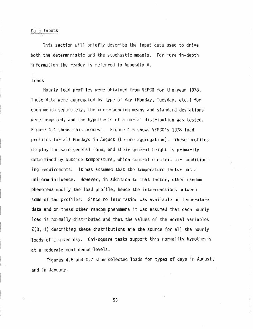
Hourly load profiles were obtained from VEPCQ for the year 1978.
These data were aggregated by type of day (Monday, Tuesday, etc.) for
each month separately, the corresponding means and standard deviations
were computed, and the hypothesis of a normal distribution was tested.
Figure 4.4 shows this process. Figure 4.5 shows VEPCQ's 1978 load
profiles for all Mondays in August (before aggregation). These profiles
display the same general form, and their general height is primarily
determined by outside temperature, which control electric air condition
ing requirements. It was assumed that the temperature factor has a
uniform influence. However, in addition to that factor, other random
phenomena modify the load profile, hence the interreactions between
some of the profiles. Since no information was available on temperature
data and on these other random phenomena it was assumed that each hourly
load is normally distributed and that the values of the normal variables
Z(D, 1) describing these distributions are the source for all the hourly
loads of a given day. Chi-square tests support this normality hypothesis
at a moderate confidence levels.
Figures 4.6 and 4.7 show selected loads for types of days in August,
and in January.
53

Yearly Load Information
(for each day, each hour)
I Aggregate
~ Loads
(by: a. type of day b. month c. hour)
--'"
I
+ Check for Normal
Distribution 2 - test X
Figure 4.4 Load Data Set-Up
54
Related Statistics

? 'S '--'
0
f I l-
L i
(OOOO!"""
I-
r
<3 5000:-...J
L
! r-
i 4000
o 12. I'" 24
TI ME
Figure 4.5 Selected Loads for Specific Days in August
55

Figure 4.6 Selected Loads for Types of in August
56

G.4-
I I I r
I
~l
,.-."
5G~ 3 ~
-...J
5-'1
0
<5 ..J
48
4-0
! j
I
lIME.
\
••••••••••• MGlDAY
-- 5ATURDA'( _.- ::>Ut-JDAY
Figure 4.7 Selected Loads for Types of Days in January
57
I l ~ I
1 I
I
-I
30

Generating and Pumped Storage Stati~ns - Generating Stations Technical
Specifications
An analysis was made of the generati uni in Virginia
Electric and Power System a~ of 1978. From the aggregated heat-rate
specifications (at 1/2, 3/4, and full power) its nuclear, coal and
oil units, the heat-rate curves were determined, as shown in Figure 4.8.
Estimated efficiency curves (Figure 4.9) inpu tput curves
(Figure 4.10) were derived from these heat-rate specifications.
The derived input-output curves contain two linear segments; one
from zero to 3/4 of full capacity output, and the second segment from
3/4 to full power. To capture this information the computer models
could be transformed to include the following in formulation:
j=2 13 '\ S * X sj Xo +.L oJ' t
J=l IJ
(4-29)
where the previous power output variable x~, is decomposed into two
power components (X~\, X~2). These components, multi ied by their res-
pective slopes (SSl' SS2)' and with the add; on of the zero-power fuel
input x~, yield the total necessary fuel input for a power output
x~l + X~2. It is also necessary to add the following constraints:
and,
j=2 I xSj - CAps < 0
j==l t
58
ft V <
::: 1 -+ 24
Is = 1 -+ 3
\t == 1 -+ 24 V <.
is == 1 -+ 3
(4-30)
(4-31)

128 4 _.- ~LlCLEA~
\ \ •·••••• .. ··OIL
-COAL i \ ~
12.4 \ \ \
IZ.O \ \. \.
11.6 \ .•••. \.
",..-..
\ .••..• \ ~r ~~ ,. ttl ... Q5 '-../
11·2 ... ,.~ ".
Ul '0 .......... ~
... . " 0. ". ti '.
0 ..... uJ •• e ................. ;. :::t 10·8
io·4
OUTPUT FRACTION
Figure 4.8 VEPCO System Heat-Rate Curves
59

~ o Q ~
31.0
30·0
~ I 2'1.0 't H rf)'
28·0
260
"..-.. -
_.- NUCLEJ\R ........... E)\L
--- COAL
OUTPUT F!<..ACTION
Figure 4.9 VEPCO System Effi Curves
60

12.
8
4
-25 -50
-- NUCLEAR. ••.•.•....•.. OIL/GAS _0- COl\L
·75
CAPACITY OUTPUT
Figure 4.10 VEPCO System Input-Output Curves
61
1.00

This would yield a deterministic model with 245 unknowns and 461 con-
straints. The increased precision would however, be minimal due to the
near-linearity of the input-output curves. Therefore the simpler
approach, as developed previously, was retained.
Using a simpler approach, we can introduce a constant 'loading
rate, or
XS _ S < k * CApS r S = 1, 3 (4-32) t Xt
_1 - S V
t = 1 24 L '
where k denotes a system constant. The computational costs of adding
another 3 x 24 = 72 constraints outweigh, however, the benefits derived
from the increased precision reached by accounting for this constraint.
Pumped Storage Technical Specifications
An average efficiency of 72% and a charge/discharge rate of 1.25
was used for the pumped storage system in the deterministic models.
Obviously, these parameters are within the control ~f the plant
designer, but they do represent acceptable benchmarks.
Cost Information
Table 4.1 contains the cost data used in this study. For
additional information the reader is referred to Appendix A. Note
that no economies of scale have been introduced in the capital cost
data since this again would create computational inefficiencies
without significant benefits.
62

Table 4.1 Costs Used in Optimization Models~
System FIXED COSTS
Capital Total Cost Fixed O&r~ Fixed Costs
($/KW) ($/KW Year) ($/1000 MW day)
Nuclear $795.00 $2.73 $194,410.96
Coal 690.00 2.50 169,068.49
Oil 440.00 1.85 108,520.55
Storage 180.26 2.18 43,013.70 (pump/ turbine)
Reservoir 8.16 0.00 1,918.39 (i n kWh)
VARIABLE COSTS
Heat-Rate Fuel Total (BTu/kWh) ($/ Variable
O&r~ Cost 106BTu) (mills/kWh) ($/1000 MWh)
Nuclear 10,400 $0.583 0.69 mills $ 6,753.20
Coal 10,100 1 .. 000 1 k1 11 71n nn .a..v. .&..&.".&.VoVV
Oil 9,500 2.730 0.30 26,235.00
Storage - - - 0.00 *2
Reservoir - - - 0.00 *2
~see Appendix A for detailed information and sources of data.
*2assumed negligable in comparision with other costs.
63
i

Simulation
To investigate the feasibility of the decision rules related to
capacity and generation loads determined by the LPS model at given re
liability levels, a simulation approach was developed. This program
calculates any deviations from the decision rules that are required
when a normally distributed load is introduced randomly. These deviations
occur when the physical constraints on storage and reservoir capacities
are exceeded.
Figure 4.11 shows the general approach to this simulation. The
time frames that were investigated included (a) a repetitive simula
tion of the peak day, (b) a week made up of the typical days of the
peak month, and (c) a repetitive simulation of (b).
64

Next Hour In Period
Normal Distribution
Z(O,l)
No Deviations
"Random" Loads
Register Deviations
Load Information
(ll and 0)
Capacity and Generation
Rules
Figure 4.11 Simulation Approach
65


CHAPTER 5
RESULTS
This chapter describes and compares the results of the model appli
cations. To recapitulate the models applied in this study, Table 5.1
lists each computer code with its corresponding features. The deter
ministic models were applied with average load profiles of each type
of day and for each month. The load profile leading to the highest
cost, i.e., the IIworstli day, was further investigated with respect to
storage and reservoir capacities. The first section presents the
details of these analyses.
The month including the "worst day" and characterized by seven
types of days was selected for the stochastic model applications .
. Again, the maximum cost day was determined among these seven days, on
the basis of normally stributed loads. The system capacities derived
on this "worst ll day were then assumed lIinstalled li in the system, and
generation sicn rules were derived for the other types of days in
this month. The second section presents the details of this approach.
Finally, these decision rules were used in a simulation to analyze
their feasibility since they were obtained through daily optimizations,
which necessarily leads to some suboptimization when these daily time
units are aggregated over a longer period .
. 67

Table 5.1 Model
Storage System Capacities Oeter- Stochas-Model ministic tic Included Excluded Unlimited VEPCa
I LPl x x x I
LPN x x x
LP2 x x x
LPS x x x
LPIV x x x
LPNV x x x
LP2V x x x
LPSV x x x
I
68

Deterministic Models
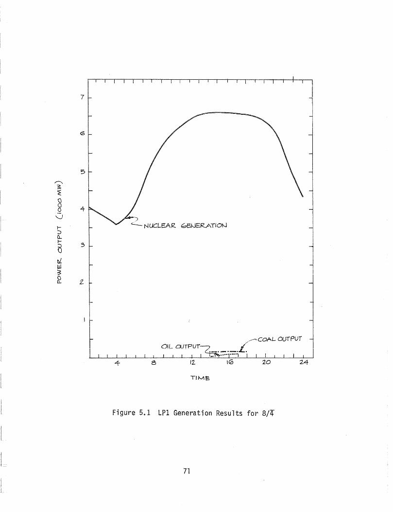
The LP1 and LP2 models were run for all seven types of days in
each of the twelve months. For both the worst day encountered was
8/4*, i.e., Thursdays in August. For the LP1 model, which excludes
storage, this selection is intuitively obvious since (a) the maximum
load in the study period occurs during the 8/4 days, and (b) installed
capacity has to be available to meet this demand. If storage is in
cluded then the maximum cost case depends on the complete load profile,
since the peak loads can be met by energy in storage derived from
generation at hours with excess capacity. However, both IIworst" cases
did coincide.
Deterministic Models Without Storage
The LP1 and LP1V models only differ in that the latter one
contains upper limits on its system capacities corresponding to the 1978
VEPCO data. The LP1 model of course is not restricted in its selection
of generation mix capacities.
LP1:
Table 5.2 contains an overview of the results obtained by the LP1
with respect to capacities and costs. Figures 5.1 and 5.2 re-
spectively show the daily generation profiles obtained with LPI
for the days with the highest load (8/l) and the lowest load (10/7).
* The notation 8/4 corresponds to month 8 and type of day 4, to distinguish it from August 4 (8/4). The types of days used are indexed by T, ... ,7 corresponding to Mondays through Sundays.
69

Table 5.2 Overview of LPI ul
Highest System
Cost Case Day* Nuclear ", Oil Total i
Capacity (103MW) 8/4 6.657 0.152 0.115
Capacity Cost ($) 1,294,252. 25, . ,SOL 1,332,418
Operating Cost ($) 890,114. 8,887. 6,459. 905,461
To ta 1 Cos t ( $ ) 2,184,366. , . ,960. 2,237,879
Lowest Cost Case
-
Capacity (103MW ) 10/7 3.616 0.047 0.274
Capacity Cost ($) 703,010. 7,980 29,734. 740,724
Operating Cost ($) 523,867. 2,763 15,914. 542,544
Total Cost ($) 1,226,876. 10, 45,649. 1,283,268
* notation: . month/type of day; where T, ... ,7" correspond to Mondays,
... , Sundays.
70
~El-JERATION
OIL ClUTPUT---, / - - -. c._ .............. L.
.--. COAL OUTPUT
I I I I , ~···T···i I I I I
4- e 12. ICO 20 24
TIME:
Figure 5.1 LPI Generation Results for 8/4
71

.--..... 4 :r ~ ~
§ v .3 ..... 2 a N UCL.f.AR OUTPUT
nL 2 ill ~
~
Figure 5.2 LPI Generation Results for 10/7
72

A regression analysis applied to the optimal capacities obtained
for each type of day in the 1978 period shows that the maximum daily load
explains 98.7% of the capacity variations for the nuclear system, i.e.,
( ~~~!~~~y in) = -.111 + .9817 (~~~~m~~) , R2d" =.987 (5-1) 1000 MW 1000 MW a J
Other variables, such as average daily load, do not improve the above
regression equation. The coal and oil capacities were also re-
gressed on maximum and average daily loads, but no satisfactory
fit could be found. This implies that they depend upon other
characteristics of the daily load profiles.
It should be noted that the load following th nuclear plants,
as illustrated in Figures 5.1 and 5.2~ may be infeasible because of
Federal regulations and uneconomic due to to resulting increases in
maintenance costs and equipment breakdowns.
This case does, however, correspond to the absolute minimum cost
case that is IIfeasible li without pumped storage.
LPIV:
The LPIV results show that the most economical generation pro
cedure is loading in the order (a) nuclear, (b) coal, and (c) oil.
Obviously this is the incremental cost loading which is expected.
Figure 5.3 shows the optimal generation schedule for 8/4, given the
VEPCO maximum capacities of 2.457 (1000 MW Nuclear), 3.288 (1000 MW)
Coal~ and 3.469 (1000 MW) Oil.
73

4
.".,-.,_. _. _ ................................................ -., / "
I \ ~ NUCLEA~
GENERATION
•.••.••••••••••• ~;OIL. .. . -.. -. -.- ..... ,
... 'III'. •
. ~\ \
OL-~~~~~-L~-L-L~~~~~~~~~~~~~ 1 12 10 20 e
TIME
Figure 5.3 LPIV Generation Results for 8/l
74

Deterministic Models With Storage
The deterministic LP2 and LP2V models incorporate the hydro
pumped storage system by the addition of hourly storage inflow and
outflow variables, as well as storage pumping and reservoir capacity
variables. The capacities are unlimited in the LP2 model, whereas the
LP2V model is constrained by the VEPCO generating capacities for 1978.
A sensitivity analysis was performed on LP2 results for 8/4.
LP2:
Introducing hydro-pumped storage in the generation system results
in an extremely levelized nuclear production and zero-power outputs
from both coal and oil generating systems, for all types of days
throughout 1978. Figures 5.4 and 5.5 present the optimum generation
patterns for the peak load type of day (8/4) and for a typical winter
day (l/T). Note that the dual peak requirements on winter days are
supplied by the storage system; not by increases/decreases in the
nuclear power o~tput. A total cost comparison between LP2 and LP1
for the peak day shows a savings of $127,414 in favor of the system
with the pumped storage. This is equivalent to an average savings of
approximately O.096¢/kWh to the consumer. Table 5.3 lists an over
view of the LP2 results. It appears that the nuclear units now exhibit
very good base loading featuers.
Regressions on the optimum nuclear capacities for each type of day
of the study period show that they are, at a rate of 99.6%, explained
by the average daily load -- not by the maximum load as for LP1. The
75

-...,J
m
Table 5.3 Overview of LP2 Results
Highest System Cost Day Case Nuclear Coal Oil Storage
Capacity (103MW) 8/4 5.732 0.0 0.0 1.652
Capacity Cost ($) 1,114,315 0.0 0.0 71,052.
Power Cost ($) 904,533. 0.0 0.0 0.0
Total Cost ($) 2,018,848. 0.0 0.0 71,052.
1..-..........-.. _- ' .... --,..-.
* Reservoir capacities in 103 MWh.
Reservoir* Total
10.720
20,565. 1,205,932.
0.0 904,533.
20,565. 2,110,465.
"'"' ............... -_ .. ""'--_. " -',~"-""

5
4
3
/ N PUT TO ':)TO!<.AGE:.
~ 2 -
I!IIIIIIIJIII---- ........... , - \
\ -- \
" .'
STO~A&E. OUTPUT
................... :;; ._0' filII
'-"''' .... " ...••..•• ~ \\\\
o 1~~~~~~~~j~\_··~~~~_~~~~~~I~I~I __ ~~ __ ~1 ~I I 4 e 12 16 20 24
TIME
Figure 5.4 LP2 Generation and Storage Schedules for 8/4
77

,..-....4 S ~ o o o ;:; :3 -
ti ill S o !l. 2
4
S NUCLEAR GeNERATION
INPUT TO ~ 5TORA&E. ,
o· ••••• " , ••••••
. 12
TIME
oTORJ\&E O~:~~~7 .. ..
. . . .
Fi gure 5.5 lP2 G·enera ti on and Storage Schedul es for 1/1
78
I
1 1 -,
I

regression fit with the average load only is:
and,
Nuclear Average () I) . Capacity in = -$038 + 1.035 (Load in . 1000 MW 1000 MW
2 R d. :::: .996 a J (5-2)
when adding the maximum load, the fit is slightly improved, ~ri th:
(
Nuclear ) (Average \ Capacity in = -.030 + 0.901 Load in )+ .112 1000 MW 1000 MW (
MaXimum) Load in , 1000 MW
R~dj = .997 (5-3)
Both the optimum storage and reservoir capacities, obtained for the
study period, are dependent upon the maximum and average daily load, i.e~:
( ~~~~~~~y in) = .170 + 1. 333 (~~~~m~I~) _ 1.393 (~~~~a~~ ) , 1000 MW 1000 MW 1000 MW
and,
LP2V;
2 Rd' = .612 (5-4) a J
,,881 + 9.522 (~~~~m~~ ) _ 10.149 ( ~~~~a~~) , 1000 MW' 1000 MW
2 Radj = .763 (5-5)
The LP2V results for the total study period indicate that VEPCO·s
nuclear and coal capacity is always sufficient to serve its system
demand. Nuclear output is completely fl at 2457 MW and coal-fired
generation follows the load profile whenever necessary. Oil is never
used in the optimal solutions. A sample generation pattern is shown
79

for day 8/4 in Figure 5.6. All the storage fllow patterns are similar
to those obtained in the LP2 applications.
;-\Pumped Stora~e Analysis'
The previous results indicate that SUbstantial savings are possible
by introducing pumped storage facilities in the system. Since site
characteristics nlay constitute major constraints on feasible reservoir
capacity, sensitivity analyses were performed by varying the maximum
reservoir capacity and the relationship between storage and reservoir
capacity was investigated. These analyses were made for the 8/4 day_
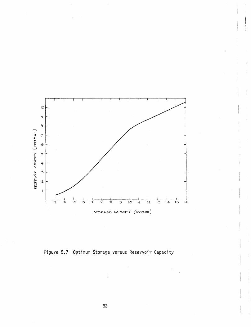
Figure 5.7 represents the relationship between the optimal storage
and the reservoir capacities when the maximum reservoir capacity is
varied continuously. Note that this relationship becomes linear when
the reservoir capacity is larger than 8000 MWh. The storage pumping
capacity (in MW) is approximately 1/7th of the size of the reservoir
capacity (in MWh). The regression fit is:
(~~~~~~~y i J 1000 MW J (
Reservoir ) . = 0.020 + 0.1389 Capacity in
1000 MWh 0.940
(5-6)
The daily system costs are shown in Figure 5.8. Given the daily
system cost without storage ($2,237,879; see LP1) the average daily
cost savings by introducing pumped storage are $21 per MWh of installed
reservoir capacity (with the corresponding storage facilities). Of
course these savings are increasing at a diminishing rate with larger
reservoir sizes.
80

4
,~ ./ ........... - .. - .. T..- .. - .. -"-~.-- ............. -"-.\ :; "./'-?COAL G.ENE.IZATIO--~ " . ..,.,.,..
\
NUCLEAR. GENERATION
_ ..... - ............ _- /,.5TORA6E INPUT
'-J \
\ \
\ ..... . \
. . . iii " flo ~ iI
eO. !It Ii • * _ ~ tit ZI (It
r5TORA&E OUTPUT
. .. .' . . . . . . . . . L-L-.~~~~L-~L-L-~~L-~L-L-~~~~~'~~~~
1 4 8 12 10 20 24
-rIME
Figure 5.6 LP2V Generation Results for 8/4
81
to
9
.\ ·2 .~ '.0 1·1 }.2. lA- 1.5 1·0
6TO~AbE.. C.APAC.ITY (1000 MW)
Figure 5.7 Optimum Storage versus Reservoir Capacity
82

2,250
~
Z'23t
~ 2/210
* .:ry '-J
~ 2)QO-0
'-..... tr5 0 \J 2,170 ::i u.l t:\ >-'fl 2,150_
2)30
2)10
IA 1.0
5TORA&E CAPACI1Y CIOOO MW)
Figure 5.8 Total Daily System Cost versus Storage Capacity
83
Stochastic M0get~_
Given the IIworstli month as determined by the previous models, the
maximum cost stochastic case was found as though this day is
neither the highest average load or maximum load day, the combined
effect of the load profile and its large hourly variations resulted
in this selection. The optimum LPS capacity and generation costs for
this day are shown in Figure 5.9 as a function of reliability. A simi-
1 ar curve is presented in Fi gure 5. 10 for the LPSV case.
The uncertainty in the hourly load yields extreme increases in the
sizes of both storage and reservoir capacities. Comparing Figure 5.11,
which shows the optimum reservoir sizes as a function of the reliability
level, with the "worstll day deterministic solution of 10 3 720 r·1Hh,
we see that the load uncertainty increases the reservoir size 4.4 times
(reliability level of 85%; 47,324 MWh) to 7.9 times (99%; 84,682 M~Jh).
The deterministic storage capacity (1,652 MW) now ranges from 3,273 to
4.524 MW for the investigated reliability range (2.0 to 2.7 its previous
size) .
From a systems viewpoint these increases are realistic since the
storage fae; 1 it; es prov; de the II buffer" for a 1'1 expected 1 cad devi at i cns.
It is however questionable whether reservoirs of this size are always
available within the utilities territory. It is also questionable
whether this size is optimum for a longer period, say a week, since it
was derived from the "worstll day case.
84

29,00
I I I I I j
85 67 8.9 31 :J5 !'5 '37 9' RELlABILI TY LEVeL l % )
Figure 5:.~9 Optimum System Cost versus Reliability Level
85

~ U 3,100
2~OO[L __ -L __ -LI __ ~ __ ~I __ ~ __ ~I~ __ L-__ ~I __ ~ __ ~I __ -4 __ ~I __ ~ __ ~ 85 B7 89 .91 ~S 35 :;)7
RELlAE:>IL ITY LEVEL (1. )
Figure 5.10 VEPCO Optimum System Cost versus Reliability Level
86

4°65 87 69 91
R.ELlA5IL1TY LE.VE.L (~)
Figure 5.11 Optimum Reservoir Size versus Reliability Level
87

The cost versus reliability curves indicated that benchmarks can
be reasonably established at the 95% and 99% levels. All further
analyses of the stochastic models is therefore made at those levels.
StoGitastic. t·.'1odel s Excludtng Storage
LPN:
Figures 5.12 and 5.13 show the power production levels for the two
reliability levels. Both plots are similar to the deterministic genera
tion pattern of LP1 (Figure 5.1). The only differences are the higher
production levels due to the added load uncertainty. Of course the
nuclear load following again seems excessive, but it can be established
as the cheapest production scenario for the most demanding day. Table
5.4 presents an overview of the LPN results.
LPNV:
The traditional economic loading rules are applicable in the VEPCO
case without storage. The generation pattern for day 8/T is shown in
Figure 5.14. The total cost of this pattern is $3,172,870, showing a
penalty (or trade-off cost) of $275,125/day as compared to the LPN
generation mix.
Stochasti"c Model s Incl uding Storage
LPS:
Table 5.5 lists the financial highlights for the LPS maximum cost
scenario. The capacities, which were determined by this 8/T configura
tion, were assumed fixed within the system, and LPS was applied to each
88

8
7
I\JUCLEAR GEt>JERAiIQI\l
4
<) I I
4- 8 12 1£0 20
TlME ('n~s)
Figure 5.12 LPN Generation Results for 8/1 at a 95% Re 1 i abi"1 i ty Level
89
24

9
TIME (HR'5)
Figure 5.13 ~PN Generation Results for 8/T at a 99% Reliability Level
90

Table 5.4 Overview of LPN Results
Highest System at 99% Reliability Level Cos't Case
Day Nuclear Coal Oil Total
Capac; ty (103MW) 8/T 8.669 0.098 0.506
Capacity Cost ($) 1,685,2780 16,501. 54,958. 1,756,738.
Power Cost ($ ) 1,095,060. 5,714. 40,232. 1,141,007.
Total Cost ($) 2,780,338. 22,216. 95,190. 2,897,745.
System at 95% Re'liability Level ~
Capacity (103MW) 8.032 0.112 0.425
Capacity Cost ($) 1,561,428. 18,866. 46,122. 1,626,416.
Power Cost ($) 1,027,965. 6,533. 33,751. 1,068,250.
Total Cost ($) 2,589,393. 25,400. 79,874. 2,694,667
91

1 -
I .. I " .I '-'"
4
J
I I I I I I I
I
/-----~::L-------------\
I \ I \ I \ I .r··... \ I .. • I ; I ! I . ·
tj NUCLEAR. : ...
GEtJERATION:'
. · · · · · · · · . . .
· · · . · · · · ·
· · · · ·
.: I I
e
.
. . . . , .
/~OIL.. . .
lZ
I I
Ita
T\ ME (loUGS)
. . . . . . .
If . . .. ..
.
· · · · · · · · . .
· · · . . . ;
· · · · I ("'! I
20 24
Figure 5:14 LPNV Generation Results for 8/1 at a 99% Reliability Level
92
]

Table 5.5 Overview of LPS Results
! 1
95% System Reliability Day
Nuclear Storage Reservoir Case Total
Capacity (103MW ) 8/T 6.619 3,857 64.457
Capacity Cost ($) 1,286,884. 165,29l. 123,654. 1,576,460.
Operating Cost ($) 1,040,421 o. O. 1,040,421. 1 I
Total Cost ($) 2,327,305 165,921 123,654 2,616,880J
99% Reliability
Case
Capacity (103MW) 8/T 6.953 4.524 84.683
Capacity Cost ($) 1,351,739. 194,594. 162,454. 1,708,787
Operating Cost ($) 1,108,711. o. O. 1,108,711
Total Cost ($) 2,460,450. 194,594. 162,454 2,817,499
93

type of day in August, leading to optimum genera on rules within
these given capacities. Table 5.6 lists the resulting costs for
August. It should be noted that this is not a complete system optimi
zation.
Figure 5.15 presents the nuclear generation pattern and the net
storage flows for day 8/1 at a reliability level of 99%. The generation
levels for day 8/1 at the lower 95% reliability level are extremely
similar.
One should note th~t in all stochastic versions of the model, a
decision is first made on generation, and the storage pool regulates
the differences between this production and the actual demand en-
countered. The net storage flows presented in gures are the
result of the generation decisions, and a demand corresponding to
either the 95% or 99% reliability level.
In all cases the decision on generation 5 almost set at the
maximum available capacity for the major part of the day. The storage
facilities are able to absorb additional energy flows as they never
reach their critical limits. The large decreases in generation during
the latter parts of the day -- because the reservoir can supply all
necessary power -- do, however, create problems concerning day to day
oeprations. This should be adjusted if a longer-term optimization is
considered.
LPSV Final Results:
Analgous to the LPS approach, the August costs are listed in Table
5.7. The generation pattern for 8/1 shown in Figure 5-16 for the 99%
reliability level and in Figure 5-17 for the 95% level.
94
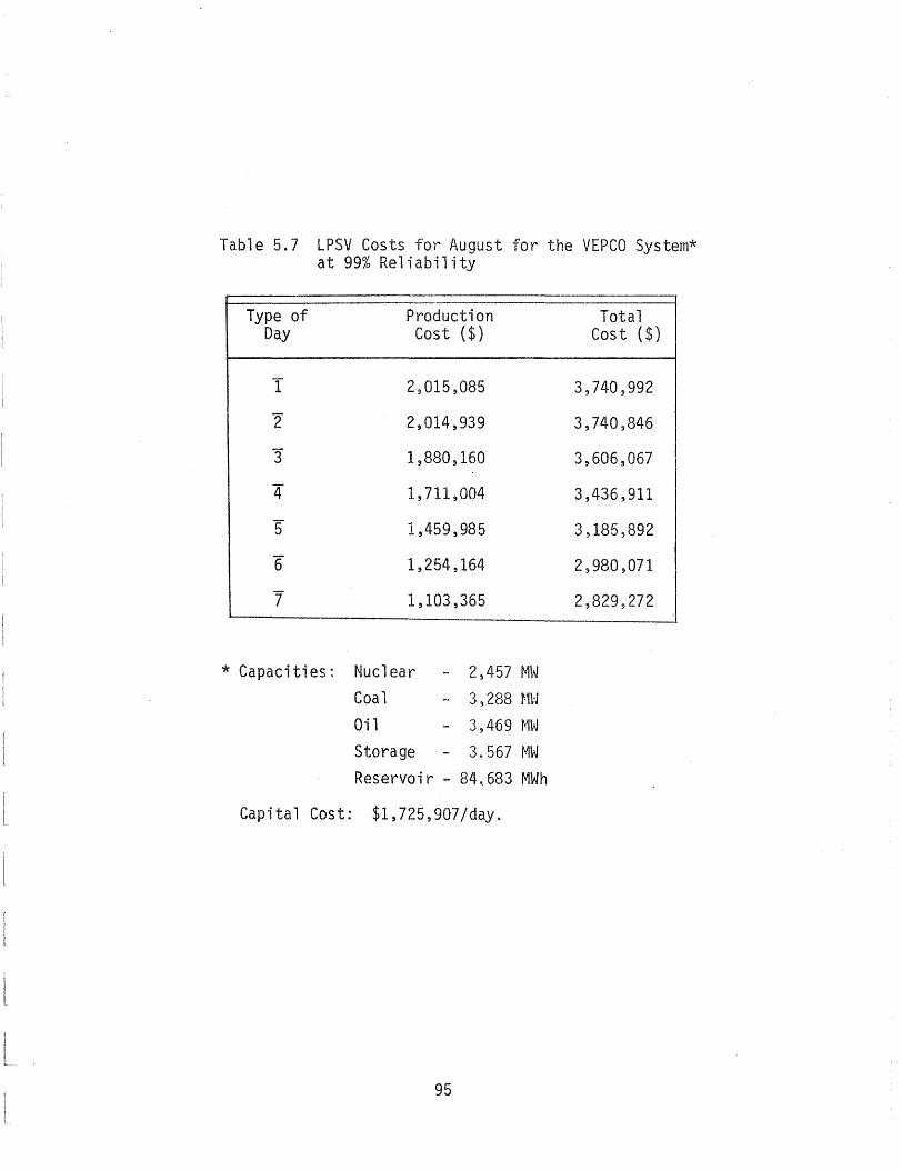
Table 5.7 LPSV Costs for August for the VEPCO System* at 99% Reliability
Type of Production Day Cost ($)
I 2,015,085
"2 2,014,939
3" 1,880,160
"4 1,711,004
5 1,459,985
"6 1,254,164
7" 1,103,365
* Capacities: Nuclear - 2,457 MW Coal - 3,288 MW Oil - 3,469 MW Storage - 3.567 MW
Reservoir - 84~683 MWh
Capital Cost: $1,725,907/day.
95
Total Cost ($)
3,740~992
3,740,846
3,606,067
3,436,911
3,185,892
2,980,071
2,829,272

Table 5.6 LPS Costs for August with Fixed Capacities* at 99% Reliabil-ity
Type of Production Day Cost ($)
T 1,108,711.
2" 1,106,20l.
"3 1,073,135.
4" 1,026,423.
5 961,051.
"6 891,827.
7 804,864.
* Capacities: Nuclear - 6.953 MW Coal 0 MW Oi 1 0 ~lW
Storage - 4.524 MW Reservoir - 84.623 MW
Capital Cost: $1,708,787/day.
96
Total Cost ($)
2,817,499.
2,814,989.
2,781,923.
2,735,211.
2,669,838.
2, , 5.
2,513,651.

B
o
-2
~UCLEAR 6ENERA110N
........... e' ••••• •••••••• ;;NE T .jTORAbE FLOW . ." . . .
'" . . . . . . . • ':-0 •••• oil' •• .. . . --_ ......... --- -_ .............. -:- ..... _ ..... _-- _ ................................... _- --;.-..&:-
.'1ilI t::I, oil· •
" " '-. .-. ",
..L I
4 I
8
.,. .......... ......
'0.
I I I I
(2. /(2,
, '\
TIME L HR.5 )
,.' ..
Figure 5-15 LPS Generation Results for 8/T at a 99% Reliability Level
97
I I
2() 24
3 -
f,-/(jCLEAR
o --------.~--
-/ I
-2 t ~,~J~I~~~~I~~~~~I~~ I I 1~,~I~~~I~
4 8 12 16 20 2..4
TIME (
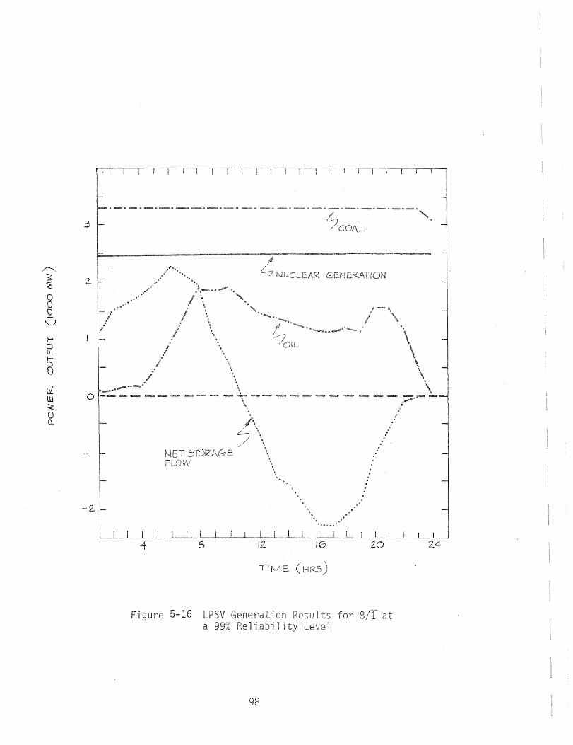
Figure 5-16 LPSV Generation 8/T at a 99% 1 'i i 1 -i
98

I I
3 .-._. _._._.-._._. - '-1-; ~O~~·-·-·-·- '_0 _._\
2.
o
-/ -
-2
-3
4 B
-'. ~'"
.... l--.lET :)To"RA0E. JO .........
FLOW \'0, . · · · · · · · · ~ ...... \ .> .... ~ 0-~ •• $. ;I
12 \(0 20
TIME lHR5)
Figure 5-17 LPSV Generation Results for 8/1 at a 95% Reliability Level
99
\
24
Simulation
The simulation approach focused on the appl"icability of the decision
rules as derived in the LPS model for reliability levels of 95 and 99%.
Given the decisions on capacity and on hourly generation for days 8/T
through 8/7, comparisons were made between the planned power outputs
and a constructed random demand. When the net storage flow exceeded
the storage capacity or the reservoir capacity, "lost power" deviations
were registered, denoted by ploss and ploss. sto ' res
Three different scenarios were investigated, namely:
(1) a long-term simulation focusi on
300 successive 8/T days;
peak day 8/T, i.e.,
(2) a simulation involving 300 successive 8/1 through 8/7 weeks,
in which the energy existing in the reservoir after hour 24
of each day is transferred to
(3) a simulation involving 300 successive 8/1 through 8/5 working
day weeks, with ihe same approach as in (2).
Table 5.8 shows the results of these simulations. To summarize this
table one should note that:
(a) for the peak-day period, the observed reliabilities are higher
than those used to specify the model IS constraints;
(b) for a total week problems do exist because of the accumulation
of energy in the reservoir, and
100

Table 5.8 Simulation Results
Required Deviations from Planned Number Reliability Generation (in 1000 MW)
of Period Level Runs ploss (in %)* ploss (in %)* sto res
300 8/T 95% 2.25 .1600 112.7 .31
99% .34 .0010 29.8 .08
300 8/T-8/7 95% 13.98 .0050 38,437.7 14.69
99% .95 .0004 47,612.3 18.19
300 8/I-8/S 95% 8.74 .0050 19,732.8 10.18
99% .59 .0003 23,912.2 .66
* % deviation represents deviation from the average hourly load level Lav9 ' where:
L (8/1) = 5,076.6 MW, avg
L~vn(8/T + 8/7) = 5,193.5 MW, and --:::J
Lavg(8/I + 8/5) = 5,384.8 MW
101
I
I

(c) these problems are mostly due to the low level demand days,
Saturday and Sunday.
The conclusion from the previous analysis is th the decision rules
should be modified if a week or a longer period is considered in the
optimization models.
102

CHAPTER 6
CONCLUSIONS AND RECOMMENDATIONS
The objectives of this study have been to determine
(1) the optimum capacities of the nuclear, coal and oil-fired
generating systems and of the pumped storage system -- in terms
of reservoir and pumping capacity, and
(2) hourly generation decision rules for each system, yielding minimum
operating and investment costs as well as high reliability of supply.
A framework was developed to derive these capacities and generation
rules, as well as to test them for a specific utility·s capacity and
load data (the Virginia Electric Power Company). The following sections
summarize the conclusions that can be drawn from this work, and list
recommendations for improvements and possible further re~earch.
103

Conclusi'ons
The general results this study, on information and
1978 cost data~ are shown below~
A. Given any 1978 ly 1
(1) pumped storage is
in the study;
(2) both storage and reservoir
explained by maximum and
leveling effect makes
systems depend compl y
'Ie 1 days considered
es can be satisfactorily
, whereas their load
the generating
load;
(J) in the optimum configuration storage ty is highly
correlated with reservoir ty;
(4) generatton i:s performed in economic loading
order, and the storage
fi.rst seven to ni:ne hours
the peak 1 ) .
11 during the
emptied during
B. Given a ca 11y determi.ned i ly load prof; 1 e:
(1) !-'Ym!J~Y storage again i for all cases
considered;
(2) the load uncertainty results tn increases in both storage
and reservoi.r capaci.ties corres to approximately
2-4 and 3-7 times the size r deterministic counter-
parts, for reliability levels ranging from 85 to 99%,
104

(3) generating costs and capital costs for an optimum system
are increasing non-linearly with the reliability of the
system, i.e. the probability of meeting a stochastic
demand pattern;
(41 zero-order decision rules can be established with respect
to generation scheduling and capacity determination.
C.. The linear programming approach for the determination of both
capacities and generation levels produces realistic solutions
which can incorporate dynamic aspects of electricity supply
(such as plant loading rates, etc.). However, the derived
decision rules do need additional adjustments since they were
obtained through daily opti,mizations, which necessarily lead to
some suboptimization when these daily time units are aggregated
over longer periods.
105

Recommendations
Recommendations for extensi'ons of the exi'sting models, and on
possible future improvements, are given
Concerning the extensions, it is recomnended that:
A. Technical information, such as plant loading rates, be
incorporated in the models to avoid severe power increases/
decreases that appeared in some outputs.
B. Losses in the pumped storage system be included in the
stochastic models to present the actual situation more
realistically.
C. More detailed input-output curves be used in all models.
Possible future improvements might focus on:
A. System optimizations over periods longer the peak-day.
B.
C.
The probabilistic formulation of the hourly loads so that:
(1) the uncertainty related to these loads can be diminished,
and
(2) the stochastic decision rules can be improved by
accounting for up-dated information.
The scheduling of maintenance and unforeseen breakdowns in a
longer-term overall optimization framework. In this case a
purchased power option is to be included in the system.
106

[ 1]
[2]
[3]
[4]
[5J
[6]
[7]
REFERENCES
Allen, A.E, IIPotential for Conventional and Underground PumpedStorage, II IEEE Transactions on Power Apparatus and Systems, Vol. PAS-96, No.3, May/June 1977, pp 993-998.
Asbury, J. G., "Central and Dispersed Storage for Utility Load Leveling," unpublished, Argonne National Laboratory, Energy and Environmental Systems Division, 1979.
Bernard, P. J., et al., IIA Method for Economic Scheduling of Pumped Hydro andSteam Generating System," IEEE, January, 1964, pp 23-30. --
California Energy Commission, California Load Management Research 1977, Report to the Federal Energy Administration, Cooperative Agreement No. CA-04-60641-00, October 1977, pp 55-60.
Casazza, J. A., et ~., II Energy on Ca 11 ,II I EEE Spectrum, June 1976, pp 44-48.
EPRI EA-970, Integrated Analysis of Load Shapes and Energy Storage, Project Report No. 1108-2, March 1979.
EPRI EL-975, Survey of Cyclic Load Capabilities of Fossil-Steam Generating Units, TPS 77-732, February 1979, Section 6.
[8J EPRI EM-264, An Assessment of Energy Storage Systems Suitable for ~lectric Utilities, Vols. 1-3, Project 225, ERDA E(11-1}-2501~ July 1976.
[9J EPRI EM-1037, Conceptual Design of Thermal Energy Storage Systems For Near-Term Electric Utility Applications, Vols. 1,2, Project 1082-1, DOE Project EC-77-A-31-1034, April 1979.
[10J EPRI FFAS-1048, Uncertainty Methods in Comparing Power Plants, Project TPS 78-797, April 1979.
[11J EPRI Journa 1, II Load Management, II May, 1977, pp 6-11.
[12J ERDA, Creating Energy Choices for the Future, ERDA-48, Vol. 2, 1978, pp. 65-69.
107

[ 13]
[ 14J
[ 15]
[ 16]
[ 17J
[ 18J
[19]
[20J
[21J
[22J
[23J
[24J
Fanshel, S. and E. S. Lynes, IIEconomic Generation Using Linear Programming," IEEE, April 9 1964~ pp 347-356.
Federal Energy Administration, Office of Conservation, Evaluation and Classification of Load Managemen!_Jquipment, FEA/D-77/209, June 1977.
Gerber, M. S., IITestimony before the Virginia State Corporation Commission,1I Contract No. 24000198, The National Regulatory Research Institute, Columbus, Ohio, June 1979
Guldmann, J. M., Extension of the Regulatory Simulation Model: Optimal Policies of Gas Purchases and Storage Operations and Expansion, The National Regulatory Research Institute, Columbus, Ohio, April 1979.
Hall, H. M., IIUtility System Power Generation Planning," unpublished, American Electric Power Service Corporation, New York, 1979.
Happ, H. H., IIOptimal Power Dispatch - A Comprehensive Study,1I IEEE Transactions on Power Apparatus and Systems, Vol. PAS-96, No.3, May/June 1977, pp 841-854.
Heuck, K., 1I0ptimal Scheduling of Termal Power Stations ,II Fourth Power Systems Computation Conference Proceedings, Grenoble, September 11-16, 1972.
Loucks, D. P. and P. J. Dorfman, II An Eva 1 uat·j on of Linear Deci s ion Rules in Chance-Constrained Models for Reservoir Planning and Operation,JI Water Resour. Res., Vol. 11, No.6, 1975, pp 777-782.
Mayer~ L. S. and C. E. Horowitz, liThe Effect of Price on the Residential Demand for Electricity,1I Energy, Vol. 4, 1979, pp 87-99.
Noonan) F. and R. J. Giglio, IIPlanning Electric Power Generation: A Non-Linear Mixed Integer Model Employing Benders Decomposition,1I Management Science, Vol. 23, No.9, May 1977, pp 946-956.
Poseidon, C., et al., IIA Study of the Transient Response to Changes in the Load ofa Utility System,1i unpublished, Department of Mechanical Engineering, The Ohio State University, August 1976.
Revelle, C. et ~, liThe Linear Decision Rule in Reservoir Management and Design," Water Resour. Res., Vol. 5, No.4, 1969, pp 767-777.
108

[25]
[26]
[27]
[28]
[29J
[30J
[31J
[32J
[33]
Sherer, C. R. and L. Joe, IIElectric Power Systems Planning with Explicit Stochastic Reserves Constraint," Management Science, Vol. 23, No.9, May 1977, pp 978-985.
Skrotzki, C., Power Station Engineering and Economy, McGraw-Hill, 1960.
Stuart, R., IICoping with Power Peaks,1I The New York Times, August 10, 1975, P 11.
Sullivan, R. L., Power System Planning, McGraw-Hill,1977, pp 96-150.
u.S. Congress, IIpublic Utility Regulatory Policies Act of 1978,11 16 USC 2601, Public Law 95-617, Sect. 101 and 115, November 9, 1978.
Vardi, J., et al., liThe Combined Load Duration Curve and its Deri vati on ,-iifE"EETransacti ons on Power Apparatus and Sys terns, Vol. PAS-96, No.3, May/June 1977, pp 978-983.
Viramontes, F. A. and H. B. Hamilton, "Schedule of Hydro Electric Storage Plant Using Dynamic Programming,1I Modeling and Simulation, Vol. 7, Part 1, ed. Vogt, W. G., Pittsburg, 1976, pp 581-586.
Windsor, J. S., IIPumped Storage Optimization in Generation Systems," Water Resour. Res., Vol. 103, May 1977, pp 99-109.
Wood, W. et al., "A Probabilistic Approach to Off-Peak Electric Energy Evaluation,1I IEEE Transactions on Power Apparatus and Systems, Vol. PAS-95, No. ·4, July/August 1976, pp 1501-1506.
109


APPENDIX A
BASIC DATA
A-I Load Data ........ .
A-2 Generating Station Data .
A-3 Cost Data . . . . . . .
111
Page
112
113
118

A-I Load Data
This study used the 1978 hourly load data of the Vtrgtnta Electric
Power Company. The hourly loads and standard devtations for the cases
described in the report are listed with the program output tn Appendix B~
In order to test the hypothesis of a normal distribution for the
hourly loads·a Chi-square goodness-of-fit test was performed. The postu
lated relation for the load distribution was:
LOAD(D,t) = LOAD(D,t) + N(O,I) * SD(D,t) (A-I)
where:
LOAD(D,t) = load on the system during type of day, D, and hour t,
LOAD(D,t) = average load during (O,t),
N(O,l) = normally distributed variable "lith mean ° and variance
1.
SD(D,t) = standard deviation of the load during(D,t)o
A more precise relationship could be expressed as
LOAD(D,t) = f(D,t,T) + N(O,o) (A-2)
where f(D,t,T) = load function depending on D,t, and on the temperature
T.
112

This approach, however, was abandoned because:
(a) no temperature data were available, and
(b) the modeling approach would have become more complex since
obviously the temperatures of successive hours are related.
The Chi-square test values show that the normal distribution assumption
for hourly loads is acceptable within an error risk of 5%.
A-2 Generating Station Data
Tables A-I through A-3 respectively show VEPCO's specifications for
their nuclear, coal and oil-fired plants. The capital cost data shown
reflect the costs as they were perceived by VEPCO in 1978. Since almost
all these capital cost estimates contain non-updated historical costs,
they are useless with respect to evaluating actual 1978 costs.
113

..p:.
Table A-I VEPCO Nuclear Unit Specifications
Capacity Unit Name (MW)
North Anna 1 907
Surry 1 775
Surry 2 775
North Anna 2 779 (not on-line till 8/79)
Summary of Nuclear Capability as of 12/78
Total Capacity Combined Heat Rates
Weighted Fuel Cost Available Capacity Average Heat Rate : WEd ghted Capaci ty Cost: Annual Cost* : Da. i ly Cos t**
Heat Rates (BTU/KWh)
Half 3/4 Full
12,000 11,400 11,300
12,000 11,250 11,000
12,000 11,250 11,000
12,000 11,400 11,300
2457 M\'J . 12,000 BTU/KWH at 50% power 11,305 BTU/KWH at 75% power 11,110 BTU/KWH at full power. 39.35 ¢/MMBTU 1,486.1 MW (or 60.48%1 11,604.7 BTU/KWH 281.24 $/KW 24.133 $/KW-year $66,118.76 per 1000 MW-day
* @ 7%, 25 years: annuity factor 0.08581 ** Annual Cost/365
Fuel Cost (¢/MMBTU)
Avg. 1/79
11,675 40.80
11,562 33.98
11,562 43.03
11,675 n.a.

--I
--I
(J1
Table A-2 VEPCa Coal Unit Specifications
Heat Rates (BTU/KWH) Capacity
Unit Name (MW) Half 3/4 Full Avg.
Mt" Storm 1 553 11,400 10,700 10,600 11,025 Mt. Storm 2 553 11,400 10,700 10,600 11,025 Mt. Storm 3 560 11,200 10,500 10,400 10,825 Bremo 3 72 12,560 12,140 12,160 12,401 Bremo 4 164 10,375 9,730 9,640 10,031 Chesterfield 1 56 16,800 16,000 15,900 16,382 Chesterfield 2 73 15,200 14,500 14,600 14,882 Chesterfield 3 100 11,600 11,050 10,950 11,308 Chesterfield 4 166 10,600 10,400 10,300 10,490 Chesterfield 5 333 11,500 11,100 11,100 11,302 Ches terfi e 1 d 6 658 11,000 10,800 10,700 10,878
Summary of Fossil Capability:
Total Capacity Combined Heat Rates
.' 3288 MW
Weighted Fuel Cost Available Capacity Average Heat Rate Weighted Capacity Cost: Annual Cost Daily Cost
11,412 BTU/KWH at 50% power, 10,880 BTU/KWH at 75% power '10,797 BTU/KWH at full power 146. 02 ¢/~1MBTU 2428.3 MW (or 73.854%) 11,128.6 BTU/KWH 149.80 $/KlfJ 12.854 $/KW-year $35,216.61 per 1000 MW-day
Fuel Cost (~/~1MBTU )
1/79
113.00
113.00 113.00
156.00 156.00
184.00
184.00
184.00 184.00
184.00
184.00 -

Table A.3 VEPCO Oil/Gas Unit Specifications -- ---------_ .. _--------_ .. _------
Heat Rates (BTU/KHH) Fuel Costs Capacity (¢!MMBTU)
Unit Name (MW) Half 3/4 Full Avg. 1/79 .b...-,.,._
Yorktown 1 166 10,400 10,000 9,950 10,190 198.00
Yorktown 2 170 11,300 11,100 11,000 11,183 198.00
Yorktown 3 818 10,390 9,940 9,830 10,145 198.00
Portsmouth 1 101 11,700 11,100 11,000 11,383 181000
Portsmouth 2 101 11,435 10,820 10,750 11,119 181.00
Portsmouth 3 162 10,180 9,795 9,900 10,029 181.00
Q) Portsmouth 4 233 10,800 9,900 9,800 10,393 181.00
-..I
Possum Pt. 1 74 13,200 13,000 13,100 13,127 175.00
Possum Pt. 2 69 13,000 12!1900 13,000 13,027 175.00
Possum Pt. 3 101 11,000 10,350 10,250 ,658 175.00
Possum Pt. Ieen. 1-6 78 15,683 15,683 15,683 15,683 299.00
Portsmouth 1,3 l.4,6 60 17,463 17,463 17,463 ,463 298.00
Portsmouth Ieen. 7-10 84 17,463 7,463 17,463 17,463 299.00
Kitty Hawk Icen. 1,2 41 17,735 17,735 17,735 17,735 299.00
Possum Pt. 4 233 10,400 9,900 9,900 10,155 175.00
Possum Pte 5 805 10,200 9,800 9,600 9,979 244.00
Lowmoo r I cen . 1-4 60 16,049 16,049 16,049 16,049 293.00 -------•.. ----.- .. - ...• -•. -.-,.---~-.-

..-I
-.!
-....J
Table A.3 VEPCO Oil/Gas Unit Specifications (Continued)
Heat Rates (BTU/KWH) Capacity
Unit Name (MW) Half 3/4 Full .-'"--_. __ ._,
Northern 1-'4 64 16,191 16,191 16,191 Surry Icen. 1,2 37 16,601 16,601 16,601 Mt. Storm Icen. 1 12 18,327 18,327 18,327
L. ______ ~ - ----- -----.•. --------.----
Summary of Oil/Gas Capability:'
Tota 1 Capaci ty Combined Heat Rates
Weighted Fuel Cost Available Capacity Average Heat Rate Weighted Capacity Cost: Annual Cost Dai -Iy Cost
3,469 MW . 11,401 BTU/KWH at 50% power 10,998 BTU/KWH at 75% power 10$912 BTU/KWH at full power. 215. 38 ¢/Mr~BTU 2,819.95 MW (or 81.290%) 11,200.5 BTU/KWH 163.43 $/KW $ 14.024/KW-year $38,421.62 per 1000 MW-day
Fuel Costs (cJ:/MMBTU)
Avg. 1/79
16,191 299.00
16,601 299.00
18,327 364.00

A-3 Cost Data
After examination of approximately 25 sources on cost information,
five were retained as realistic -- based on discussions with utility
executives and utility consultants. Four of these, and their cost esti
mates, are presented in Table A-4. The actually used estimates, plus
the fifth source concerning hydro pumped storage and reservoir, are
presented in Table A-5.
118

--' --' (,,()
Table A-4 Considered Cost Estimates
Ca~ital Cost ($/Kw) Fue 1 Costs
System 1* 2* 3* 4* 1* 2* ($/MMBTU) ($/MHH)
Nuclear 795. 700. 779. 719- .583 7.3
Coal 690 625. 315 ... 605- 1.000 17.0 475. 721
Oil 440. 424. 334. n.a. 2.730 29.6
Pumped Storage 250. 319. 185- n.a. 0.000 0.0
1120.
1* National Power Grid Study (NRRI) 1977 year-end $. (12/78)
2* Evaluation & Classification of Load Management Equipment (6/77), 1981 $.
3* Progress in Optimal Scheduling (9/77)
4* EPRI Journal (10/77); 1976 $.
3* 4* ($/MWH) ($/t~MBTU)
4.2 .49-.63
11.0 .83-1.07
20.7 n.a.
0.0 n.a

Table A-4 Considered Cost Estimates (Continued)
3* Progress in Optimal Scheduling (9/77)
4* EPRI Journal (10/77); 1976$.

Table A-5 Cost Estimates Used in Study
----"I i
Cap; tal Cap; ta 1 Cost *3 F"ixed O&M Total Fixed Costs Total Fixed Costs $/kW $/kW-year $!kW-year $/k\.tJ-year $/103 t4W-day
Nuclear *1 795. 68.23 26 73 70.96 194,410.96
Coal *1 690. 59.21 2 c 50 61.71 109,068.49
Oil*l 440. 37.76 1.85 39.61 108~520.55 N I *2 Storage 180.16 13.52*4 2.18 .70 ,013.70
Reservoir *2 8.16*5 0.70 0.00 0.70 1,918.39 ,-~---~---
*1: National Power Grid Study; 12/78
*2: EPRI-EM 264
*3: @25 yea rs; 7%
*4: @40 years; 7%
*5: in $/kWh
All costs &re expressed in 1978 dollars.


N U1
CUT PUr-FuR MljNfH- R , ANJ D,AY 4 SENSITIIIITY ANALYSIS
TIME POWER OUTPUTS (luC)O MWH)
NUC LEAR COAL OIL STO .OUT STD. INPUT STD. POwEi< K:::SEF'~iJlk JEMANCI
l~--- -Z-;451 1.623 OeO 0.0 0.0 c.e --o-.;-u-- 4~C2;:; 2 2 .. 451 1.402 0.0 0.0 0.0 v.l: c:.o 3.[1~4 3 2.457 1 .. 273 0.0 0.0 0.0 0.(, G.~ 3.13(, 4- Z.457 t!! Z05 gaO &"8 828 8. 0 c.r 3,,65~ 5 2.457 ~.32 .. 0 • .' .0 0.(\ :o.Tn (:, 2 .. 4 57 1 • 692 G • GO. 0 O. (i 0 • 0 ;, " G 4. 14 ~ 7 2 .. 457 2.308 C.O 0.0 0.0 0.0 ).C 4.76'::> S 2.457 2.810(.0 o.G,c.e __ 0.0 ,~,,() :.267 9 2 ,,4 57 ~4Q-~-----o.O-~--~---'-O;;O----" ~---(').;O~ u.C ;,-;;-0------ '].~ '7 G 6
10 2 .. 457 3~288 G.3D1 0.0 0.0 0 .. 0 G.C: 6.052 11 2.457 3.238 0.511 0.0 0.0 o.C' J.O 6.256 12 2.457 3.28P. C.6fi,6. 0.0 0.0 O.CQ.CJh.43l 13 7~S7 ---~28 8 - ~-q 12 {)~{)-- U';-O- G; (, (; -. 0 6 • b 5 'f 14 2 .. -457 3 .. 2A8 1.('68 0.0 0.0 G.C 0.0 6.313 t~ 2.457 3.288 1.121 0,'.9 OsO 9. 0 9·9 h."l46
_ 2.451 --+:1qB iOtA (J.~ 0'8 UiC ll.~ LeG'! 7 2 .. 451 .L88. 79 c. o. 0.0 o. 6.C!24
18 2~457 3.288 1.C64 o .. Q 0.0 0.0 o.e 6.209 19 2 .. 457 30288 0.734 0.0 0.0 0.0 c.o 6.52'i 2(L 2 .. 457 3.288 0 .. 765 0.0 0.0 G 0 f.O 6.51C 21 2.451 -3.288 0.480 0:0 '0:0'- ---~ ~() .. ;)~() ~e225 22 2.457 3.135 0.0 0.0 0.0 0.0 ,).0 5.592 23 2.457 2.476 C.O 0.0 0.0 0.0 :.C 4.933 24 .z....!tll 1 .. 892 Oe Q ~_C 0.0 C.G 0.,0 4.349
CAPACITY lon~ "MW-=------ 2 .. 457 3-.--Z~B'--'- .. r.TT9--------- -cr;1)~- ~--:-----.-'-~---o_;u lTmTI.Jr+Jm

N (j)
~T FOR MoNtA 8 f AND DAY 4 SENSITIVITY ANALYSIS
l'UiE____ PO WERi CO ST S L$'~OOfr--,t.U4Hl~_AN~_" OF TOT H
NUC LEAR COAL OIL TOTAL
1 16592.12 4,6.~' 2 16592.12 50.3~} 3 16592 • 1 2 5: 4 16592~r2~( 5,1t. 5 16592.12« 51.8%) 15456~03 48.2%) 0.0 o.o~n .. ___ . 6 16592.12 (4'5.6:t) 19812 .. 15 54.4%) 0.0 o.o~n 36404.27 1 165q2&12« 38.0%} 21030*20 62.0%) ~$O OeO%) 4362:?32
~ 19~~~:t ~-r-~-6:~ l ~~:lll~---g-:-g-f---g-:grr- ~Z~~E6~ 10 16592 .. 12 (26.3't:1 61.0'f,) 8046.28 (12 .. 7'1:) 63140.88 11 16592 12 f 2.L.2U... 56.2%1 13398.22 { 1g e 6'tl 6849;'"Q? 12 16592 .. 12 I' 2;~.n) 52.7%) 17994.59 ( 24 .. 6:d 13089.19 13 16592.12 21 .. ca) 4'3.U) 23934.19 I 30.3%) 1902f>..79 14 16592.12 J 20000:i 46 .. 3~) 28021.6 33~7~ 83116 .. 21 15 16') 92 .1. Z ~ 19. WL 45g...5....1;1 R 4 4'" _3*,,3~9-.I.P76.....,.+7'7--2 ____________ _ 16 16592.12 19 .. 4% 45~l% 3 28 • 6 .5. 85371.66
18 165"42.12 20.Ctl 46.4%} 27916.67 33.65;,) 8311.27 11 16592 .. 12! 19.3% 44 .. 8%) 30938 .. 94· ! 36 .. 0~) _ 86833 .. 54
19 16592 .. 12 2' 1'1 c:; '" ~~._~Q..Q...22--_ 20 16592 .. 12 (22.1%) ( 20061~91 (Z6~7~) 75156.'51 21 16592.12 (2'+- .. 5%) ( 12595 .. 43 ! 18~6%) 67690.03 22 16592.12 (31.1%) ( 68 .. n) o .. u« o .. o~o ''13299.46
Z} 1952Z II f ~!t:-M) I g1:~~ 8:8 f 8:8i~ .....;1;;rn~.....,igi#f8..y.:~rl-~----------·
"({IT ALS 398210 ~g 7 ---.1..41'52.4. .. 29 _ _ _ __ 2..626 39 • 62 1408373.18

B-1 LP1 Output
B-2 LP2 Output
B-3 LPS Output
APPENDI X ,B
SELECTED OUTPUT
123
Page
124
127
131

-.I
N ..J:::o
'SYSTEM DATA INPUT INf'ORMATION
N~-------- --uJAl-- --UT~ STDRAG£
MJ:X-;--uurPUT···~------- -l-;-UU- T~OO -T;OO 1.00
POWER CO STS U/I000 MWH):
STORAGE «EFFI CIENCY): (CHARGE RATE) g
6753.00 11110.00 26235.00 0 .. 0
0.72 le25
O.BJECIIVEFUNCTIOl'fCOST:)! (FUEL': 6753.00 11710.00 26235 .. 00 0.0
to I
(CAPACITY): 194410096 169068.49 108520.55 43013" 10 (RESERVOIR): 1918.39 r
MCNTH DAY
8 4
'"0 I-'
UFMANtJ INFORMA I ION ---0 C
LOADS FOR 1 TO 24 HRS. IN MW. .+ '''0
4234 .. 60 4014.00 3884~20 3813 .. 80 5860.20 6206.40 6410.40 6585.60
"t: r+
__ . _____ .. 1079.00 6963.80 6693060 6664 .. 40
3<131.60 6812.00 6379.80
4303~60 6961,,80 5146.40
4<120.00 7000.60 5087.20
'5421.20 7054.00 4504.0u
LOAD INFORMATION fl000 MW) TIME TOTAL LOAD MAX .. L DAD AI/G. LOAD LOAD FACTOR
DAY 132 .. ,815 6.924 5.534 0 .. 799

.......!
N '-I
SYS TE M rybTA-l1'!PUI I "IFOR Mil TTOl'\J
----mJCU A R roll.: 0 r [ ~rrRAGE
MAX. DUTPUT-FRAClIUN: 1.00
POWER COSTS U/IOOO MWH):
STORAGE (EFFI CIENCY): (CHARGE RATE);
OBJ E CTIVe-FU1~TION --cUSTS: (FUEL): «CAPA ClTY »: tRE SERVO I R» :
6753.00
6753.00 194410096
1.00 --------- 1.00 1.00
11710.00
11110.00 169068,,49
26235.00
26235.00 109520.55
0.0
0.72 1.25
0.0 43013.70
1918.39
M{J\JTH DAY
IJE1"IAND INFORMA nON
LOADS FOR TO 24 HRS. IN MW ..
8 4 423·4- .. 60 4014 .. 00 38 84~ 20 3813.80 3931.60 4303.60 4920.00 542192C 5860.28 6206 .. 40 6410 .. 40 20-r9_,,-O__ 6963@80 6683.60
6585&60 6812$00 6967 0 80 7000.60 7054.00 666lt-~ 40 1;.319_~80 5746.40 5067.20 4504.v0
LO AD I NFORMA TI ON !l 000 MW)
TIME TOTAL LOAD MAX.L OAD AVG. LOA D LOAD FACTOR
DAY 132 .. 915 6.924 5.534 0.799
o:J
r -0 N
o C rl"

--' N 00
un POI FOR MON-m--T-, ,6..W1 DAY 4 SENSITIVITY ANALYSI~
TIME POkER OUTPUTS nooo MWH)
NUC LEAR COAL OIL STO.OUT STO.INPUT STO.POWER R( SER 1101 R. DEMAND
r------Z-.. 7i5T ~-~ .. 229 0.0 0.0 1.6C6 lT~u-- -1;'523 4.eso 2 Z.4C;7 ;1.008 000 0 .. 0 1.606 0.0 ~·.047 3 e O?9 3 2.451 ,~.e78 0.0 0.0 1.6('1(', o.c 4.57) 3.730 4 2.457 ;~.80R 0.0 o.c 1.6G6 C.O 6.094 3.65Q ., 2.451 £.926 G.O 0.0 1.606 ------u-;-c;----;-- ·---7~b17 3.1"0 6 2 .. 451 3.289 0.0 0.0 1.596 0.0 9.132 4.149 1 2~457 ~~.268 0.0 0.0 o.Qeo 0.0 10.061 ~.165 8 2.457 3.288 0.0 0.0 0.478 0.0 lC.51') '5.20 9 2.451 ~~.28R 0.0 U;U--~------U-;U39 o.e -10;'55~ 5.1(,6
10 2.457 ~t.238 0.0 0.323 0.0 0.307 Iv.n9 6.C52 11 2.451 3.2~8 0.0 O.S3~ 0.0 0.511 9.691 6 .. 2~,6 12 2.457 ~.288 0.0 0.723 0.0 O.6~6 ~.9hq ft.43l 13---- ~--7_;,<t..,,___ j .. 2138 0 .. 0 IJ.'TEZ------U-;U-- - O.Gl12 8. OC 6 6 .. 651 14 2 .. 457 3.238 0 .. 0 1.126 0.0 1.068 6.880 6.a13 15 2.457 3 .. 233 0.0 1.160 0.0 1.101 '5.720 6.846 16 2.457 : •• ~·89 0.0 1.211 0.0 10154 4."(.3 6.399 17 ~~---Z-';4 5~-6 .. 288 0 .0 1. 243 -u-;u--------r;TT'7-----);?ElT-----b-. .. 24 18 2.457 3.288 0 .. 0 1.122 0.0 1.064 2. De 6 .. t!09 19 2.451 30.288 O~O 0.826 0.0 0.784 1.312 6.529 20 2.457 3..288 C.G O.8C6 OeO 0.765 0.'506 6.510 21 2 .. 457 3.239 o;u--- O .. 5Cc~---U_.U O~-~,----- {;~OGr., --6.225 22 2.451 3.135 0 .. 0 0.0 C.O O.G 0.000 5.592 23 2.451 2:.416 0,,0 0.0 0 .. 0 0.0 0.000 4.933 24 2 .. 451 1.892 O~O 0.0 0 .. 0 0.0 O.OOC 4.349
CAPACITY 1000 MW;2 .. 457 :3 ,,288--- - U-"O . 1 .. 600 10.553 n 000 MWH I

--' N !..O
rrTnJGTiFGR-~n~IR 8, ANa DAy 4 SENSITIVITY ANAU'SIS
II ME PO WE~ cos, :;,_,..!.1,;!!.$.!.,./.!;..1 ~C~C~C-!M:!.!W~H.!...I)w't......::A).!.;N~D:..-...:li%~O~f---.!.T.l:.!O..!..T!:..A=-L _________________________ _
NUC LEAR COAL OIL TOTAL
, 1 165 92 e 1 2 (30 .. 5% ) 378 09 03 3 (6 9. 5 % ) 0 5 () O. 0 % ) '54 401 • 4 5 2 16592.12« 32.0t) 35226.11 ! be.O'll 0.0 0.0%) 51818.23
! i&~~~:i~ f B:~1+-ffigY:'1 I gI:~H 8:8 8:8il 19H~:~l 5 16592.12 (32.6t) 34261.20 (67 .. 4%) 0.0 O.O~O 50853.32 6 16592.12 (30.1%) 385L2.48 (69.9%) 0.0 O.O~) 55094.60
--.7 __ -.l659~3LIL _L30al',O 38502.48 L69.9%} 0 .. 0 O.Oi:) 5"i094.6G a 16592~·r2--{-3o.TI') 3~502.4P. 'T-~ 0.0 ~~--"5'094--;--6"O 9 16592.12 (30.1~1 38502.48 (69.9%) 0.0 (O .. C~) 55094,,60
10 165Q2e12 (30 .. VO 38502.48 (6'1.9%) 0.0 f 0.0"0 55094.60
. '12 16592 .. 12 30;-~) 38502.48 (69.9 C.u (O.O%) '5~(,94.60 ~ 165n.12 f3~;1 38~W.4S I 60.91'~~~Q~.~g~(~~Q.~o~r~)~~~"I~~,Q~Qi~ •• ~6~0~~~~~~--~~~~~~~
13 16592.12 30 e VO 38502.48 (69.nl c.o (O.C'O 5')(94.60 14 16592 .. 12 (30"n:) 38502.48 (69 0 9%1 0.0 (0 .. 0:0 55094.60
ft-t~~9~:t~ f ~8:tH-~~~~ 8:8 f 8:8H ~~8gt:g8 11 16592 .. 12 (30 .. ro 38502~48 «69.9%) 0$0 I O.GlI 5':;094.60 18 16592 .. 12« 30.1'0 38502.49 (69.9~) 0.0 (O.G't) 5"1G94.60
__ 19 16592a12 t 3Qml:O 3g502~48 (69.9%) .,O~O_ .L....D.otl 5')('94.60 20--------u;-S92 ~ 12 30 G 1': ) 38502.48 69.9't} ---0;0-( --O'Ul:1-----550C14j'cO 21 16592.12 30 .. VO 38502.48 69.9:0 O.O! O.Ot} 5'50 Q 4.60 22 16592 .. 12 31.1%) 36101.34 68.9%) 0.0 IO .. O't) 53299.46 23 16592f~2 36.41:i 28988.11 63.6'f:J 0.0 (O.C't1 4')",80.23 24 16592 .. 12 42 .. 8% 22158.84 51.2% 0.0 I 0.0%) 39750.96
_UJTAlS 398210 .. 87 8"11118.3_4____ 0 • 0 127598<'.41

-..a W o
~TR 8, ~fl\ll)DAY - --4 SENSITIVITY ANALYSIS
COST SUMMARY;ALl IN $
POWER COST CAP Q COST TOTAL COST
NUCLEAR 398210 .. 87 ~17661 .. 69 ____________ Si5a1JL .. 55
COAl 871778 .. 5.4 555897.21 1433675 .. 76
OIL 0.0
STORAGE« IN) 0.0
S TaRA GE( OUT , o. Cr
RESERVOIR
0.0 O~O
6Ci076.01
2024,3 .. S5
69016 .. 01
(J.O
20243.85
TOTALS cT275989~ 4;y-----------rrzZ1J!1lt;7l; Z39 8874.17

-I
W
-----.------MAjf~-oOipUr_ -f'fACflCHiC-----
POWER COSTS (~/I000 ~WH}:
- ------- -----SfORAGF----_-_·_· (EFFICIENCV': (CHARGE RATE.:
-- ---.------. ----OBJfCflve-FliNC ;ft CNtOSt S : (FUF.L': (CAPACITY):
-. ____________ .lRES_ERV_OH~»: _
NUCLEAR
1,.-00
6153 .. 00
6753 .. 00 194410.96
SVSTFM DATAIMPUT INFOR~AT!O~
COAL
1 .. 00
11110 .. 00
11710.00 169068 .. 49
OtL
L.OO
26235 .. 00
26235 .. 00 11)8520 .. 55
DEMAND iNFOPMATION
MONTH nAY LO'&OS FOR 1 T(l 24 I-RS. IN MW ..
R 1 3666.67 3530 .. A3 3453 .. 8 3 3431 .. 50 3601 .. 17 4008 .. 17 4632 .. 66 5438 .. 83 5755 .. 50 5923 .. 16 5q72 .. 66 6243 ... 50 6312 .. 16 6414 .. 83 6470 .. 5J 6384 .. 83 6156 .. 00 6191 .. 50 5999 .. (:6 5410 .. 50 4165 ... 16
STANDARD DEVIATIONS IN MW.
" 1 4i.~ .. 32 392.37 341 e 60 331 .. 93 303 .. (5 243 .. 42 282 .. 32 497.41 586 .. 90 145",66 839 .. 14 969 .. 21 lO1:l .. 12 1018 .. 13
11·.3 .. 27 10~7.26 1035 .. 86 88q .. 97 803 .. 29 720 .. 97 628 e87
LOAD INFORMATION (lCOO MW)
tiME TOTi\l LOAD MAX.LOAD AVG.lOAO LOAD f~CTOP
DAY 121 .. 839 6.323 5 .. 077 0.803
- ---STrUU.GE
T.)O
0 .. 0
0 .. 72 1 .. 25
0 .. 0 43013 .. 10
__1918.3q-_
5085 .. 33 6471 .. 66 4219 .. 5:1
333 .. 89 1145 .. 52
577 .. 13
OJ I
W
~

-J
W N
-----OlJTPUtFlJR-m"iNTH-----~f-;-.in,lI)OAy 1-- - ;STOCHASTIC ANALYSIS WITH PElIA8IlITV lEVEL OF q!)-t---
TIME POWfR OUTPUTS (1000 MWH) NUClrAR-----ToA[------orr------- --- - NSF
---t- ~:-~~~-----g:-g----------g:g.------- -. 2.131 2.319 2.495 3 6.4 7 5 0.0 0.0
4 6.472 0.0 0.0 5 ,6.6.1_9 _______ .. _0 .. () _________ ,_. _0 .. 0 ____ . _______ _
16 6 .. 619 0.:) 0.0 1 6.619 0.0 0.0 8 6.619 0.0 0.0 q 6.619 o.~. _.0 .. 0 ----ro f. 619----0.0- ---.- ----~~- -- 0 .. 0-
11 6.619 0 .. 0 0.0 12 6.619 0.0 0.0
_______ 13__ __6.619 __________ 0 .. 0 0 .. 0_ 14 6.619 0.0 OeO 15 6.619 0.0 0.0 16 6.619 0.0 0.0
__ 17 _____________ 6" 619 _____ _ _____ 0 "'_:)__ __ ______ _ 0 .. 0 18 60619 0.0 0.0 19 6~619 OeO O~O 20 6.619 J.O 0.0
.21 6 ... 619 _________ 0.0 _ _ 0 to 0 22 6.619 0 .. 0 OeO 23 6 .. 061 0.0 0 .. 0 24 2.934 0.0 0.0
CAPAC lTV 1000_ ~W: _ 6 .. 619 0 .. ) 0.0
2 .. 533 2 .. 513 2.289 1.588 1 .. 034 0 .. 360
-0.132 -0.611 -0 .. 844 -1 .. 369 -I .. 524 -1 .. 154 -1 .. 949
__ ":,,L .. 931 __ -1..742 -1 .. 412 -1 .. 162 _,,:,,0 .. 800 --0.050
0 .. 224 -2.262
3.857
----- --,rE SERVOIR - -DEMANO' -- . --- CfI:=VT'A-TnJN
2. 131 - ------4.-"51 6 .. <;45 9. ~7A
12 .. C51 14.340 15.<;28 16 .. S62 17 .. 323
--- 17 .. 191 16.~80 15 .. 736 14 .. 361 ~12 .. E43 11 .. eA9
9 .. 141 1.203 5 .. 462 -4 .. 049 2 .. 88A 2 .. (88 2 .. 038 2 .. 262
-O .. COO
64 .. _458
3 .. 512 0 .. 863 -- 3 .. 3 16 -- - ~ ~- -~ --- 0 .. 16"9-3.299 0.681 3.271 0 .. 662 3 .. 452 0.594 3 .. 853 ---O .. 41r----4.418 0.553 4=931 0 .. 654 5.284 O .. Q75 -- -5 .. 60 1 ---- ----- ~ L. 1 5-0--5.15R 1.461 5 .. 81 8 1.,,646 6.089 1~900 6 .. 151 -1.:986 60260 2 .. 113 6 .. 323 2 .. 245 6 .. 316 2 .. 241 6 .. 2 3 o--~- -2., 13 r-----------6.001 2 .. 030 6.031 1 .. 144-5 .. 845 1 .. 574-5.256 1.413 4.610 1.233 4 .. 065 1 .. 131
0000 MWH.'

w w
- oot~~t FeR MONTH 8 , AND DAY 1 ;STOCHASTIC ANALYSIS WiTH RELIABILITY LEVEL OF 95 ~
TIME POW~R COSTS (S/I000 MWHt, AND ~ OF TOTAL
NUCLEAR COAL all
------1---4;r937:33 ---(f(jo-~o'~.--------{)~-o-- -( 0.,0%'-0 .. 0 2. 43654.67 (100 .. 07:) 0 .. 0 (o .. o~, 0 .. 0 :3 43121.25 (lOO.O~) J .. O (o .. o~n 0.0
________ 4 ____ 43104.4.5 __ tloo .. o~n _____ 0.0 {O .. O'J;L 0 .. 0 5 4'.700.81 (100 .. 0:~) 0.0« o .. o~, 0 .. 0 6 44700 .. A 1 ( 1 00. O'ln ) .. 0 ( a .. 0 % ) 0 .. 0 1 44100.81 (100.0%) 0.0 (a.or) 0.0
_______ 8 __ "4470_C. .. 81 __ tlOO .. O~~) ________ 0 .. o ___ t __ 0 .. O~ ) ________ 0 .. a 9 44700 .. 81 nOQ .. o~n 0.0 {o .. o~n 0 .. 0
10 44700.81 (IOOoO~' 0.0« OeO~' OeO II 44700 .. 81 (lOO.O%} J .. O (0.0%) 0.0 12. ______ 44700 .. 81_tl00.0~n _______ 0 .. 0_ --L 0 .. 0%) 0.0_ 13 44700.81 (lnOeO~) OeO« 0.0%' 0.0 14 447 .J 0 .. 8 1 « 1 0 0 .. ()~n a .. 0 ( 0 .. 0 %) 0 .. 0 15 44700.81 (100 .. 0%) 0.0 I 0.01) 0.0 16 ____ 44_700.8L __ { 100 .. O~gL _________ ),,0 ____ t _ 0 .. 0%>' _____ 0 .. 0 1 7 44 7 0 0 .. 8 1 ~ (100 .. 0 ~n 0 .. 0 ( 0 .. 0 % l 0 .. 0 18 44100 .. 81 {lCO .. mn 0 .. 0« o .. o~, 0 .. 0 19 44100 .. 81 (lao .. o~n J .. O (O .. ot) 0 .. 0 20 _____ 44-10 0 ... 8_L_l1 00 .. 0% ) ______ -<1 .. 0 . (_ 0 ... o~a__ _0 .. 0_ 21 44700.81 (lOO .. O~) 0.0« o .. ot» 0 .. 0 22 44700 .. 81 (100.01) 0 .. 0« 000%) 0.0 23 40Q73 .. 01 (lOOem:) Q .. O« o .. o~n 0 .. 0 2.4 ____ ~_80.9.-",~LIOO ___ 01U ___ . ____ J .. o L ___ O,,_O%L _____ .. 0 .. 0_
lOT~lS1040421 .. 22 0 .. 0 0 .. 0
« o .. o~, « O .. O~O ( O .. O~) ( 0 .. 0% L ( 0 .. 0%) « 0 .. 0%' « 0 .. 01;)
_( __ O .. O~L ____ . « O .. O~) ( 0 .. 0'1;) « 0 .. ,)'l';) (o .. o~) ( 0 .. 0%) ( 0 .. o~u ( 0",0'1") L __ a .. O~) _ { O.O~) ( 0 .. 0'" ( o .. cun ( _____ O .. O~) __ « o",o~n ( 0. o:u « o .. o~t L_ 0_ .. 0'(1. ___ _
TOTAL
43931 .. 33 4361)4 .. 61 43721 .. 25 43704 .. 45 44700 e Al 44100 .. 81 44100 .. 81 447JO .. 8L 44100 .. 81 44700.,81 447)0 .. 81 44100 .. 81 447)0 .. 81 44100 .. 81 44700.,81 44700 .. 81 44700 .. 81 44100 .. fH 44700 .. 81
__ 44700 .. 81 __ __ 447'10 .. 81 44700.,81 40973 .. 01 19809 .. 95_
1040421 .. 22

....... w ..j:::::.
--:----OUTPUTFOf-l --MONTH- ---8--;- -AND-DAY 1 ;STO(HASTIC ANAlYStS- WfTH REliABILiTY LEVEL O~ --tj5-~
NUCLEAR
COA,l • otl
STORAGE
RE SERVOI R
TOTALS
_._------_._-_._-- .--.-.. -- -- _ ..
COST SUMMARY;All IN t -----~---- .. _--- .. _ ..
POWEP COST CAP. (OST
1040421~22 1286883.qi 0;.-(,------- -----0 .. (,------
000 0 .. 0 0:,-0- --- -----16 5921-~ 04
123654.63
1040421 .. 22 1516459 .. 59
TOTAL COST
2321305 .. 13
0.0
0 .. 0 165921.tf4 ---
123654 .. 63
2616880 .. 8 C

w ()1
--- - ---- --_ .. - ------- ---------~------- . ----- sv 5T,=", t'lATA YNPUT INFORMAl I ml
.. -.--- -----NUC lE A R-- COAL OIL - - - - --------sTORI\Gl:
~AX. OUTPUT FRAcTION: 1 ~OO--- 1 .. 00 -·-r .. oo-POWER COSTS (S/1000 MWH,: 6753 .. 00
--- r-.;Oo---
11710.00 26235 .. 00 0 .. 0
STi"fRAG"E (EF~ Ie [HICY) : (CHARGE RATE.:
0 .. 12 1 .. 25
OBJECTIVE FUNCTION-c1rsn:------_·-·---- ------.-.- -(FUEL): 6753 .. 00 11710.;00
16906Q .. 49 26235.00 OsO
(CAPACITYt: 194410 .. 96 ______ ..JL(.!..O.R-"'-E-"-S ..... E'-'-R~Q.iJ~J_: ________ . ________ ._. __
lO~520.55 43013.70 _____ ________ ._1918 .. 39 ____ _
- -- ---._----------- ---- - - -~-OEMANDINFOR~ATrON
~ONTH DAY L OAI)S FOR TO 24 t-RS. IN MW .. --~----- --.-- - ---------- ~-
R 3666 .. 67 3530 .. ~3 3453 .. 83 3431.50 3601.17 4008 .. 17 4632 .. 66 5085 .. 33 5438.83 51'55 .. 50 5923 .. 16 5972 .. 66 6243 .. ~o 6312.16 6414 .. 83 6471 .. 66
-- --------_._-.- _ 6410 .. 5-)_ 6384 .. 83 _6156 .. 00 6191 .. 50 5999 .. 66 5410.50 4165 .. 16 4219 .. 50
ST A~lDAPI! DEVIATiO~lS HI MW ..
A 440.32 392.31 347 .. 60 337 .. 93 303.(5 243 .. 42 282 .. 32 333 .. A9 4<H .. 41 586. 0 0 145 .. 66 839 .. 14 96q.21 1013 .. 12 1078 .. 13 1145 .. 52
1143.21 1081.26 1035.86 889.C;7 803 .. 29 120 .. Q1 628 .. 87 511 .. 13
LOAD INFOP~ATION (1000 MW)
lIMF 'tOTAt lnAD MAX. LflAf) AVG.lOAr LOAD ~A(TOR
f) AY 121 .. 83 q 6.323 5.017 0 .. 803

w m
(jfjfpiJTf! o~--MoNfH 8 -, -~~ID f) Ai>( - 1 ;STOCHASTtC A~AlVSIS WI1H RELIABILITY lEVEL OF - q9-~
TIME POWER OUTPUTS (1000 MWH'
f\lUCITAr tOlll ----o1r---
~ !:-~S-3-------g:8----------- -8:-8-3 6 .. 978 0.0 0 .. 0 It 6.931 !J .. J J • .) ~ ~-:~~~--- ----- 8:g ------- 0_ .. 0 6 0.0 1 ~ .. 953 0 .. ) 0.0 8 6.Q53 0.0 0 .. 0 9 6.953 0 .. 1) - 0 .. 0
10 6 ~--953 ------- --0.0 - ----- ----- - 0 .. 0 11 6.951 0.0 0.0 12 6 .. 9'53 0 .. ) 0 .. ,)
----rt--------~-: 2~ ~---- --- -8 ~ g 0 .. 0 0 .. 0
15 6.C)S3 1.1 0 .. 0 16 6.9~3 OeO 0.0
-t-k-----i:-~~}- ~---- --8:6 --- 0 .. ') 0,,0
19 6 .. 953 0,,0 0 .. 0 23 6 .. 953 0 .. ) 0 .. 0 2L ________ 6 .. _953 ____ _ 0 .. ') 0 .. 0 22 6 .. 953 0 .. 0 0 .. 0 23 6 .. 953 0 .. 0 0 .. 0 24 4.423 0 .. 0 0 .. 0
CAPACITY _l..O_J_Q._t.'IWL __ _6 .. _953 ____ _ __ O.J 0 .. 0
NSF R~Sr:RVOIR
2.256 -- 2.256 2.501 4 .. 1(-,0 2.734 1.4c)4 2.784 1 I'J. 277 2.720 12 .. <;97-2.413 15.410 1. 14~ 11 .. 21A 1.163 18 .. 381 0.38Q 18.169
-0.15C) IS.tIO -0.136 11 .. P.74 -1.027 16 .. ~41 -1.632 15 .. 2P5 -1 .. 813 13 .. 407 -2 .. 083 11 .. ~1C) -2.320 8 .. «;99 -2 .. 301 -- be 692
---2 .. 071 't- .. t 16 -1 .. 116 2.<;00 -1 .. 375 1 .. 1524 -0 .. 9(;0 O .. ~64 -0 .. 159 0 .. 405
0 .. 123 1 .. 128 -1.12B -OoCOO
4 .. 524 84.f83
nEMANO
3 .. 512 -3.116 3 .. 2c)9 3.217 3.452 3. A5 3 4.418 4 .. 931 5,,284
- 5 .. f.Ol - -
5 .. 768 5 .. 818 6 .. 089 6 .. 157 6 .. 760 6 .. 323 6 .. 316 6 .. 230 6 .. 001 6 .. 031 5 .. 845 5 .. 256 4 .. 610 4 .. 065
(l000 "4WH .. '
-DFVTAT1UN---
1 .. 1'34 -'1 .. 0-10--
0 .. 895 0.810 0 .. 180 0 .. 6 27 ------- ---0 .. 127 0 .. 860 1 .. 281 1 .. 511------ ---- -- -1 .. 920 2 .. 162 2 .. 496 --- 2.6)9- - ---------2 .. 116 2 .. 950 2 .. 944 --- -2 .. 800--------------2 .. 667 2 .. 292
_2 .. 068 1..856 1 .. 619 1 .. 486
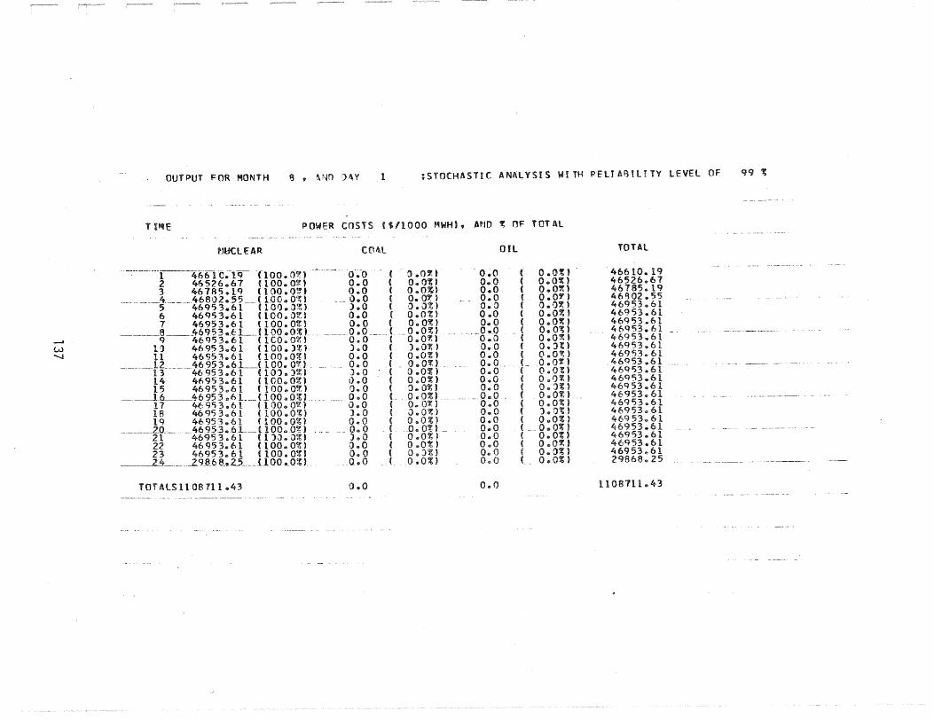
W "'-J
OUTPUT fOR MONTH 8 , &,1\10 ) 1\ V 1 ;STOCHASTIC ANALYSIS WiTH PELYABYLTTV LEVEL OF
T tflltE POWER COSTS (1/1000 MWH), AND ~ OF TOTAL
tJutLEAR
1 46-61-'::i~T9 -flOO. ()~n 2 46526.67 (100. osq 3 461A5.1q (lOO.O~t
______ 4. ______ 46802 .. 55 ___ « 1.00. OQ~) 5 469S3.61 (100.0%) 6 46953.61 (100.0t) 7 46953.61 (lOO.O%l
_____ 8~ __ 46953._6L_.« 1 00 .O~g) 9 46953.61 (ICO.O%)
1') 46953 .. 61 (lOO.)~~) 11 46~53.61 (100.0%)
______ 12 ______ 46953 ... 6L_tlOO .. O'f) _ 13 46t;l53 .. 61 (lO,) .. )~~) 14 46953.61 (lOO@O%) 15 46953 .. 61« lOO .. O~e)
_--.1_~_46 95 3,,6 L ___ (100 .. 0%»._ 11 46953.61 (lOO.O~) 18 46953.61 (lOOeO~) 19 46953.61 (100.0%)
. ___ 20. __ 46.953 .. 6_1._«- 1 OO .. O~) 21 46953.61 (110.0%) 22 46953 .. 61« 100 .. ot) 23 46953Q61 (100.0%)
____ ~ ____ ._.2.9J:t6 8..25 ____ 1..100 .. 0:&)
TOTAlSII08111.43
cnal
o~-o « C) .. 07.) 0.0 « 0 .. at I 0.0 ( O .. O~)
___ 0 .. 0 ( o.or) ).0 « 0 .. J%) 0.0 (0.01';) 0.0 « O. 0~10
_____ 0 .. 0 ____ ( __ o .. 0%) 0 .. 0 ( o .. o~n J .. 0 ( ) .. ow, ) 0.0 ( o .. O%} 0 .. 0 « 0 .. O'-f:) .),,0 ( o .. o~n 0 .. 0 « 0 .. 0%) Q .. 0 ( 0 .. 0%) 0 .. 0 «0 .. 0%) 0 .. 0 ( 0 .. 0%) ) .. 0 « J"O~) 0 .. 0 ( o .. o~n
_0 .. 0 .. ( _o .. o~n_ ) .. 0 ( 0 .. 0%) .) .. 0 ( 0 .. 0%) 0 .. 0 ( O .. J~)
__ Q .. O . ( 0 .. 0%)
0 .. 0
OIL
- 0.0 ( O .. O~) 0 .. 0 ( 0.0") 0.0 « O .. O~) 0.0 ( 0.0'" 0.0 ( 0 ... :)7; ) 0 .. 0 ( 0.02';' 0.0 ( O.O<J:)
. __ 0.0 - ( 0. O~) 0 .. 0 ( o .. o~q 0.,0 « O .. Jtl 0.0 « (\ .. O~) 0 .. 0 _ L 0 .. 0'1') 0 .. 0 ( O.Ot) 0 .. 0 ( O.i)'f:) 0 .. 0 ( O .. J~'
__ 0 ... 0 _ « _O"O~) 0 .. 0 ( O.O~) 0 .. 0 ( J .. O~) 0 .. 0 ( O .. O~) 0 .. 0 (. 0 .. O~) 0 .. 0 ( 0 .. 0%) 0 .. 0 « O .. O~) 0 .. 0 « o .. o~} 0 .. 0 t O .. _O~ )
0 .. 0
TOTAL
46610 .. 1C} 46526 .. 67 46185 .. 19 46902 .. 55 46953 .. 61 46953.61 46953 .. 61 46953 .. 61 46953,,61 46953 .. 61 46953,,61
_46953.61 469'>3 .. 61 46953.61 46953 .. 61 46953 .. 61 469')3.61 46953 .. 61 46953 .. 61 46953 .. 61 46953 .. 61 46Q53 .. 61 46953 .. 61 298M3 .. 25
1108111 .. 43
99 1.:

...... W 00
OUTPUT FOP -MO~TH 8 ? AND D ~y 1 ~STOCHAST(C A~IAlVSIS WITH RElIABlllTV lEVEL OF
COST SU~~ARV;All iN S -----". - .•... - --------------_ .. --_ .. _._-----
POWER COST ._._ •... _-_._--------------•.. _------ - .. -
NUCLEAR 1108711.43 , - -CO A[---------------------O ~-(j- ----
OIL 0 .. 0
CAP. COST
1351139.42 0.0-
0.0 --SfORAGE-·------cf;()----~---·- -- - -- ----1945qj ~ 99
RESERVOIR 162454.26 -----. -~-.-----. -----~.---.----
TOTALS 110e711.~~3 1108187 .. 66
- .. --------- -------.---- ------- -" .-.---- .---
-------------.. ". -- ~ ... _-- ---_ .. -
TOTAL COS t
2460450.85 -0.-0--
0 .. 0
1945q3 .. 9~
162454.26
2811499.0C;
qq :c