an application of hydraulic tomography to a large-scale fractured

An Application of Hydraulic Tomography to aLarge-Scale Fractured Granite Site, Mizunami,Japanby Yuanyuan Zha1,2, Tian-Chyi J. Yeh2, Walter A. Illman3, Tatsuya Tanaka4, Patrick Bruines4, Hironori Onoe5,Hiromitsu Saegusa5, Deqiang Mao6, Shinji Takeuchi7, and Jet-Chau Wen8,9

AbstractWhile hydraulic tomography (HT) is a mature aquifer characterization technology, its applications to characterize hydrogeology

of kilometer-scale fault and fracture zones are rare. This paper sequentially analyzes datasets from two new pumping tests as wellas those from two previous pumping tests analyzed by Illman et al. (2009) at a fractured granite site in Mizunami, Japan. Resultsof this analysis show that datasets from two previous pumping tests at one side of a fault zone as used in the previous study ledto inaccurate mapping of fracture and fault zones. Inclusion of the datasets from the two new pumping tests (one of which wasconducted on the other side of the fault) yields locations of the fault zone consistent with those based on geological mapping. Thenew datasets also produce a detailed image of the irregular fault zone, which is not available from geological investigation aloneand the previous study. As a result, we conclude that if prior knowledge about geological structures at a field site is consideredduring the design of HT surveys, valuable non-redundant datasets about the fracture and fault zones can be collected. Only withthese non-redundant data sets, can HT then be a viable and robust tool for delineating fracture and fault distributions over kilometerscales, even when only a limited number of boreholes are available. In essence, this paper proves that HT is a new tool for geologists,geophysicists, and engineers for mapping large-scale fracture and fault zone distributions.

1State Key Laboratory of Water Resources and HydropowerEngineering Science, Wuhan University, Wuhan, China.

2Department of Hydrology and Water Resources, University ofArizona, Tucson, AZ, USA.

3Department of Earth and Environmental Sciences, Universityof Waterloo, Waterloo, Ontario, Canada.

4Obayashi Corporation, Tokyo, Japan.5Japan Atomic Energy Agency, Mizunami, Japan.6Department of Geophysics, Colorado School of Mines, Golden,

CO, USA.7Department of Geosystem Sciences, Nihon University, Tokyo,

Japan.8Research Center for Soil and Water Resources and Natural

Disaster Prevention, National Yunlin University of Science andTechnology, Douliu, Taiwan.

9Corresponding author: Department of Safety, Health andEnvironmental Engineering, National Yunlin University of Scienceand Technology, Douliu 64002, Taiwan; 886-921-824183; fax:886-5-537-6916; [email protected]

Article Impact Statement: Kilometer-scale hydraulic tomog-raphy can complement geological mapping to yield more detailedhydrogeological characteristics of fault zones.

Received August 2015, accepted March 2016.© 2016, National Ground Water Association.doi: 10.1111/gwat.12421

IntroductionThe characterization of detailed hydraulic properties

of the fracture/fault zones is crucial to water resourcesand environmental issues. Approaches that quantitativelycharacterize hydraulic properties in fault zones and/orfractured rocks have evolved rapidly over the past fewdecades. For example, Hsieh et al. (1985) adopted aclassical analytical solution based on an equivalenthomogeneous media conceptual model to analyzedata from 20 cross-hole pumping tests. They obtainedanisotropy in K for the bulk equivalent homogeneousfractured rock, without delineating the spatial distributionof hydraulic parameters and fractures. Using single- andmultiple-well hydraulic tests at a site near Mirror Lake,New Hampshire, Hsieh et al. (1999) determined locationswhere fracture zones intersected individual boreholes andthe degree of hydraulic connection between boreholes. Atthe same site, Day-Lewis et al. (2000) used a simulated-annealing algorithm to generate three-dimensional (3D)realizations of fracture-zone geometry conditioned to(1) borehole data, (2) inferred hydraulic connectionsbetween packer-isolated borehole intervals, and (3)an indicator (fracture zone or background K bedrock)variogram model of spatial variability. Day-Lewis et al.(2003, 2006) subsequently combined geophysical data

NGWA.org Groundwater 1

and a conventional hydraulic test (a cross-hole test, nothydraulic tomography [HT]) as well as tracer tests at thesite to characterize the fracture-rock aquifer heterogeneity.

After the 3D HT simulation work by Yeh and Liu(2000), HT laboratory experiment by Liu et al. (2002),and transient 3D HT analysis by Zhu and Yeh (2005),exploring the possibility of high-resolution mapping offractured medium using HT, has become an activeresearch area. For example, Brauchler et al. (2003) usedHT to map the diffusivity of a single fracture in a largecore sample through laboratory experiments. Hao et al.(2008), using numerical experiments, showed that HT canmap the fracture pattern vividly, including its intercon-nectedness. Similarly, Ni and Yeh (2008) demonstratedthe usefulness of pneumatic tomography (PT) for imagingfractures based on numerical experiments. More recently,Sharmeen et al. (2012) confirmed in the laboratory theefficacy of HT to detect fractures and their connectivityand reported that the estimated K and S s could accu-rately predict the drawdown behavior in other pumpingtests not used in the inverse modeling effort. Overall, thefield applications of 3D HT work are still limited (Cardiffet al. 2013), and there are only a few HT field applica-tions in fractured media (e.g., Lavenue and de Marsily2001; Meier et al. 2001; Vesselinov et al. 2001; Illmanet al. 2009; Tiedeman et al. 2010).

With a pilot point method, Lavenue and de Marsily(2001) analyzed datasets from seven boreholes inducedby a series of sinusoidal pumping tests and availablegeologic facies data to characterize the K field in theCulebra-fractured dolomite formation within the DelawareBasin in southeastern New Mexico. Likewise, Meieret al. (2001) interpreted drawdown and recovery datasetsfrom seven boreholes induced by two cross-hole pumpingtests and one steady-state head dataset during non-pumping periods to map preferential flow paths in asubvertical shear zone in granitic rock at the Grimselrock laboratory (Switzerland). For mapping fractures inunsaturated media, Vesselinov et al. (2001) examinednumerous cross-hole pneumatic injection tests at theApache Leap Research Site (ALRS) in Arizona.

Based on the detailed site-scale subsurface stratigra-phy in a fractured-aquifer in West Trenton, New Jersey,Tiedeman et al. (2010) developed a three-dimensionalflow model consisting of predetermined 33 horizontaland inclined layers in addition to a known fault zonenear a boundary. In line with the suggestion by Yehand Lee (2007) for HT, they then took advantage of thegroundwater level data collected at 44-48 monitoringwells or intervals due to temporary shutdown of threepumping wells in a pump-and-treat operation to calibratethe K values of each layer of the model.

A recent comprehensive review by Illman (2014)emphasized that the accurate characterization of detaileddistribution and the connectivity of fractures in a geo-logical medium has been a technological challenge fordecades. Based on many different studies conductedaround the world, Illman (2014) concluded that HToffers much improved imaging of heterogeneity and, in

particular, connectivity of hydraulic parameters in com-parison to traditional mapping methods such as kriging,stochastic simulation, and stochastic inverse modeling ofsingle-pumping tests.

Nonetheless, the scales of most of the previousinvestigations were limited to fractured media of meters totens of meters. Very few cross-hole pumping or injectiontests have been conducted in a tomographic fashion overthousands of meters in fault and/or fracture zones, exceptfor those by the Japan Atomic Energy Agency (JAEA).During the past decade, JAEA installed several verticaland inclined boreholes over an area of several squarekilometers at depths of up to 1 km to characterize thehydrogeology near the Mizunami Underground ResearchLaboratory (MIU) site in central Japan. The site is situatedin a fractured and faulted granite formation (JAEA 2010).Two pumping tests during 2004-2005 were conducted atdifferent depths along one borehole, and responses of thesaturated granite formation were monitored using packed-off intervals at various depths within different boreholes.

With these datasets, Illman et al. (2009) estimatedthe hydraulic conductivity (K ) and specific storage (S s)tomograms as well as their uncertainties and delineatedthe large-scale connectivity of K and S s at the site basedon a sequential successive linear estimator (SSLE) (Zhuand Yeh 2005). They showed that the results of theiranalysis qualitatively corroborated well with observeddrawdown records, available fault information, and coseis-mic groundwater level responses during several largeearthquakes (e.g., Niwa and Takeuchi 2012). However,they suggested that estimated fracture pattern and faultlocations may still involve large uncertainty due to onlytwo pumping tests, with limited observations for inversemodeling.

Over the past few years, two large shafts for theunderground laboratory were excavated at the MIUsite. During the process of the excavation, groundwaterwas drained, and responses at all previously installedmonitoring locations were monitored. In addition, a newpumping test was conducted in 2010 at a new boreholelocated at the vicinity of the shafts, and responseswere collected with existing and additional observationboreholes. As these new datasets become available, wethus ask how much improvement can be obtained forthe characterization of hydraulic parameter fields at thesite as Illman et al. (2009) only used the data from twopumping tests. Furthermore, they used a uniform meshand a relatively small computational domain, which mayhave led to undesirable boundary effects. Therefore, thispaper aims to assess improvements of the estimated K andS s fields and patterns of fractures and faults at the MIUsite using all data collected with new pumping locationsand new observation boreholes. It also studies the impactsof selected domain size and boundary conditions as wellas prior geostatistical information.

Description of the Field Site and Pumping TestsA detailed description of the MIU site geology can

be found in Saegusa and Matsuoka (2011). According

2 Y. Zha et al. Groundwater NGWA.org

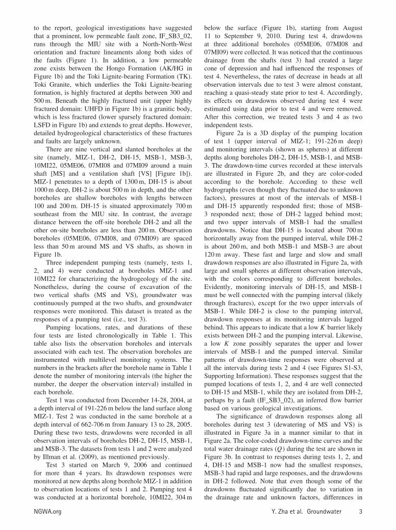
to the report, geological investigations have suggestedthat a prominent, low permeable fault zone, IF_SB3_02,runs through the MIU site with a North-North-Westorientation and fracture lineaments along both sides ofthe faults (Figure 1). In addition, a low permeablezone exists between the Hongo Formation (AK/HG inFigure 1b) and the Toki Lignite-bearing Formation (TK).Toki Granite, which underlies the Toki Lignite-bearingformation, is highly fractured at depths between 300 and500 m. Beneath the highly fractured unit (upper highlyfractured domain: UHFD in Figure 1b) is a granitic body,which is less fractured (lower sparsely fractured domain:LSFD in Figure 1b) and extends to great depths. However,detailed hydrogeological characteristics of these fracturesand faults are largely unknown.

There are nine vertical and slanted boreholes at thesite (namely, MIZ-1, DH-2, DH-15, MSB-1, MSB-3,10MI22, 05ME06, 07MI08 and 07MI09 around a mainshaft [MS] and a ventilation shaft [VS] [Figure 1b]).MIZ-1 penetrates to a depth of 1300 m, DH-15 is about1000 m deep, DH-2 is about 500 m in depth, and the otherboreholes are shallow boreholes with lengths between100 and 200 m. DH-15 is situated approximately 700 msoutheast from the MIU site. In contrast, the averagedistance between the off-site borehole DH-2 and all theother on-site boreholes are less than 200 m. Observationboreholes (05ME06, 07MI08, and 07MI09) are spacedless than 50 m around MS and VS shafts, as shown inFigure 1b.

Three independent pumping tests (namely, tests 1,2, and 4) were conducted at boreholes MIZ-1 and10MI22 for characterizing the hydrogeology of the site.Nonetheless, during the course of excavation of thetwo vertical shafts (MS and VS), groundwater wascontinuously pumped at the two shafts, and groundwaterresponses were monitored. This dataset is treated as theresponses of a pumping test (i.e., test 3).

Pumping locations, rates, and durations of thesefour tests are listed chronologically in Table 1. Thistable also lists the observation boreholes and intervalsassociated with each test. The observation boreholes areinstrumented with multilevel monitoring systems. Thenumbers in the brackets after the borehole name in Table 1denote the number of monitoring intervals (the higher thenumber, the deeper the observation interval) installed ineach borehole.

Test 1 was conducted from December 14-28, 2004, ata depth interval of 191-226 m below the land surface alongMIZ-1. Test 2 was conducted in the same borehole at adepth interval of 662-706 m from January 13 to 28, 2005.During these two tests, drawdowns were recorded in allobservation intervals of boreholes DH-2, DH-15, MSB-1,and MSB-3. The datasets from tests 1 and 2 were analyzedby Illman et al. (2009), as mentioned previously.

Test 3 started on March 9, 2006 and continuedfor more than 4 years. Its drawdown responses weremonitored at new depths along borehole MIZ-1 in additionto observation locations of tests 1 and 2. Pumping test 4was conducted at a horizontal borehole, 10MI22, 304 m

below the surface (Figure 1b), starting from August11 to September 9, 2010. During test 4, drawdownsat three additional boreholes (05ME06, 07MI08 and07MI09) were collected. It was noticed that the continuousdrainage from the shafts (test 3) had created a largecone of depression and had influenced the responses oftest 4. Nevertheless, the rates of decrease in heads at allobservation intervals due to test 3 were almost constant,reaching a quasi-steady state prior to test 4. Accordingly,its effects on drawdowns observed during test 4 wereestimated using data prior to test 4 and were removed.After this correction, we treated tests 3 and 4 as twoindependent tests.

Figure 2a is a 3D display of the pumping locationof test 1 (upper interval of MIZ-1; 191-226 m deep)and monitoring intervals (shown as spheres) at differentdepths along boreholes DH-2, DH-15, MSB-1, and MSB-3. The drawdown-time curves recorded at these intervalsare illustrated in Figure 2b, and they are color-codedaccording to the borehole. According to these wellhydrographs (even though they fluctuated due to unknownfactors), pressures at most of the intervals of MSB-1and DH-15 apparently responded first; those of MSB-3 responded next; those of DH-2 lagged behind most;and two upper intervals of MSB-1 had the smallestdrawdowns. Notice that DH-15 is located about 700 mhorizontally away from the pumped interval, while DH-2is about 260 m, and both MSB-1 and MSB-3 are about120 m away. These fast and large and slow and smalldrawdown responses are also illustrated in Figure 2a, withlarge and small spheres at different observation intervals,with the colors corresponding to different boreholes.Evidently, monitoring intervals of DH-15, and MSB-1must be well connected with the pumping interval (likelythrough fractures), except for the two upper intervals ofMSB-1. While DH-2 is close to the pumping interval,drawdown responses at its monitoring intervals laggedbehind. This appears to indicate that a low K barrier likelyexists between DH-2 and the pumping interval. Likewise,a low K zone possibly separates the upper and lowerintervals of MSB-1 and the pumped interval. Similarpatterns of drawdown-time responses were observed atall the intervals during tests 2 and 4 (see Figures S1-S3,Supporting Information). These responses suggest that thepumped locations of tests 1, 2, and 4 are well connectedto DH-15 and MSB-1, while they are isolated from DH-2,perhaps by a fault (IF_SB3_02), an inferred flow barrierbased on various geological investigations.

The significance of drawdown responses along allboreholes during test 3 (dewatering of MS and VS) isillustrated in Figure 3a in a manner similar to that inFigure 2a. The color-coded drawdown-time curves and thetotal water drainage rates (Q) during the test are shown inFigure 3b. In contrast to responses during tests 1, 2, and4, DH-15 and MSB-1 now had the smallest responses,MSB-3 had rapid and large responses, and the drawdownsin DH-2 followed. Note that even though some of thedrawdowns fluctuated significantly due to variation inthe drainage rate and unknown factors, differences in

NGWA.org Y. Zha et al. Groundwater 3

IF_SB3_02

DH-15

MIU Site

MIZ-1MSB-1

10MI22MSB-3

05ME06

07MI0807MI09

(a)

DH-2

MSVS

DH-2

Test 1

Test 2

DH-15MIZ-1

TK

UHFD

LSFD

Miz

unam

iG

rou p

(S

edim

enta

ryLa

yer )

Tok

igra

nite

IF_SB3_02

Low KBarrier

Flow Barrier

MSB-1MSB-3

Test 4

Test 3

10MI22

Pumping interval

(b)

VS MS

05

ME

06

07

MI0

8

07

MI0

9

Monitoring section

AK/HG: Hongo Formation

TK: Toki Lignite–bearing Formation

UHFD: Upper highly fractured domain

LSFD: Lower sparse fractured domain

950 m

510 m

Figure 1. (a) Map of lineaments and faults obtained on the basis of the geological and seismic surveys in the vicinity ofthe MIU site, where borehole locations as well as the locations of the main shafts (MS) and ventilation shafts (VS) areshown (modified from Illman et al. [2009]). (b) A schematic cross-section showing the boreholes, the pumped and observationintervals as well as the local geology along the dashed line connecting DH-1, MIZ-1, and DH-15 in a. The dashed curvesapproximately delineate the contact among various geological units.

responses are apparent. As indicated by the sizes of thespheres in Figure 3a, responses at the observation intervalsof MIZ-1 varied with their locations, in particular, largeresponses at deep intervals (for drawdown-time curvedetails, see Figure S17). Responses from this test suggestthat the two shafts are likely linked with MSB-3 andDH-2 but separated from DH-15 and MSB-1, perhaps bythe low K barrier (IF_SB3_02).

HT AnalysisTo quantitatively interpret the observed groundwater

responses during the four tests, we use the SimultaneousSuccessive Linear Estimator (SimSLE) algorithm (Xianget al. 2009). SimSLE takes all the available pumping testsinto consideration simultaneously to estimate the three-dimensional K and S s spatial distributions as well as their


Table 1The Detail of the Four Pumping Tests

Pumping location(s)

Test no.Average pumping

rate (m3/d) Period start Period endBorehole

nameDepth

intervals (m)Observation

intervals

1 14.4 December 12, 2004 December 28, 2004 MIZ-1 191-226 DH-2 (1-12)DH-15 (1-10)MSB-1 (1-5)MSB-3 (1-7)

2 7.2 January 13, 2005 January 28, 2005 MIZ-1 662-706 DH-2 (1-12)DH-15 (1-10)MSB-1 (1-5)MSB-3 (1-7)

3 5581 March 9, 2006 — MS&VS Change with time DH-2 (1-12)DH15 (1-10)MIZ1 (1-10)MSB1 (1-5)MSB3 (1-7)

4 288 August 11, 2010 September 9, 2010 10MI22 304 DH-2 (1, 5, 9, 12)DH15 (1-10)MIZ1 (1-3)MSB1 (1-5)MSB3 (1-7)

05ME06 (1-11)07MI08 (1-7)07MI09 (1-4)

1The average pumping rate from MS and VS for the first 15 days.

uncertainties. The algorithm and the computational costof SimSLE are presented in Supporting Information forinterested readers.

Data Utilized in the HT AnalysisIllman et al. (2009) excluded data that did not exhibit

clear responses to pumping from the upper intervals ofMSB-1 and MSB-3 during tests 1 and 2 because of theirvery small signal-to-noise ratios. However, we found thatthe upper intervals showed small but consistent responsesduring the four pumping tests. Thus, they were includedin the current HT analysis. Although all tests lasted fora long period of time (Table 1), we only used datacollected over the first 14 days for test 1 and 15 daysfor the other three tests. While drawdown data collectedduring longer pumping tests may carry information aboutheterogeneity at great distances, their usefulness for thisinvestigation is limited. This is because most of theboreholes were clustered at the center of the MIU site(near field), and only a limited number of monitoringintervals were installed at one borehole (DH-15) at afar distance (far field). Thus, it would be difficult tointerpret the large time drawdown as it likely representsthe effects of heterogeneity anywhere within or beyond thesimulation domain, unless more observation boreholes atdifferent locations were available.

Domain, Mesh, and Boundary ConditionsDifferent from the previous work (Illman et al.

2009), which employed uniform grids and a relatively

small three-dimensional domain (884 × 392 × 1054 m),this analysis adopted a larger three-dimensional domain(2000 × 2000 m in horizontal directions and 1400 m inthe vertical direction). In addition, an adaptive meshgenerator was developed to discretize the simulationdomain. This irregular 3D mesh for the simulation isillustrated in Figure S4 along with the locations of thepumping and observation boreholes and intervals. Thismesh discretization resulted in 43,470 nodes and 47,112elements. The corresponding computational and storagecosts for this inverse modeling effort are discussed in theAppendix S1.

For the HT analysis, we assumed that groundwaterwas hydrostatic prior to the beginning of each cross-hole pumping test. Constant head boundary conditionswere assigned to the lateral boundaries, while the topand bottom were treated as no-flux boundaries. Diagnosticsimulations indicated that different boundary conditionsdid not affect the inversion results as we deliberatelyselected a relatively large domain and short simulationtimes for the inversion.

Prior InformationThe prior information for SimSLE includes the mean

K and S s as well as their correlation scales. For thisHT analysis, the guessed mean and variance valueswere the same as in Illman et al. (2009) (i.e., meanK = 0.01 m/d, mean S s = 2.3 × 10−6 1/m, variance oflnK = 2.0, variance of lnS s = 0.5). The mean or effectiveK and Ss values (representing some average properties of


Q=14.4 m3/d

t (d)

Dra

wd

ow

n(m

)

0 2 4 6 8 10 12 140

0.05

0.1

0.15

0.2

DH-2(1-12)

DH-15(1-10)

MSB-1(1-5)

MSB-3(1-7)

(b) Drawdown vs. time curves

Figure 2. Observed drawdown responses induced by cross-hole pumping test 1. (a) 3D borehole plot and (b) drawdownvs. time curve. In a, the size of the sphere reflects the relativesignificance of the drawdown recorded at each monitoringinterval (see the interval number near the sphere) of eachborehole. In b, the lines with the same color denote responsesfrom different intervals of one borehole. The colors of thesphere correspond with the colors of the hydrographs. Thecube indicates the pumped location. Q is the pumping rate.More detailed drawdown curves are presented in Figure S15.

matrix, fracture, and fault) were derived from traditionalcross-hole pumping test analysis. Generally, such priorinformation, based on the unimodal distribution statistics,is often considered inadequate to characterize the bimodaldistribution of K for a fracture medium (e.g., Tsofliaset al. 2001). Nonetheless, according to Yeh and Liu(2000), prior information about mean, variance, and

Time (d)

Dra

wd

ow

n(m

)

Q(m

3/d

)

0 5 10 15

0

2

4

6

8

DH-2(1-12)

DH-15(1-10)

MSB-1(1-5)

MSB-3(1-7)

MIZ-1(1-10)

(b) Draw down vs. time curves

1000

Q from MS and VS

500

0

Figure 3. Observed drawdown responses induced by cross-hole pumping test 3 (a) 3D borehole plot and (b) drawdownvs. time curve. In a, the size of the sphere reflects the relativesignificance of the drawdown recorded at each monitoringinterval (see the interval number near the sphere) of eachborehole. In b, the lines with the same color denote responsesfrom different intervals of one borehole. The colors of thesphere correspond with the colors of the hydrographs. Thecube indicates the pumped location. Q is the pumping rate.More detailed drawdown curves are presented in Figure S17.

correlation scales does not play an important role inHT analysis for a porous medium if a large number ofspatial observations (such as in HT analysis) are available.For fractured medium, the effects of initial estimates(means, variances, correlation scales, and correlationfunctions) had been investigated by Meier et al. (2001).They concluded that the large-scale heterogeneity patternsestimated from different initial guesses were similar but


could introduce great uncertainty when they were usedin solute transport prediction. We also investigated theinfluence of initial guesses (shown in Figures S9-S10 inthe Supporting Information), resulting in similar findingsas those from Yeh and Liu (2000) and Meier et al. (2001).

Results and Discussion

Estimated Parameter Fields Using Data From FourPumping Tests

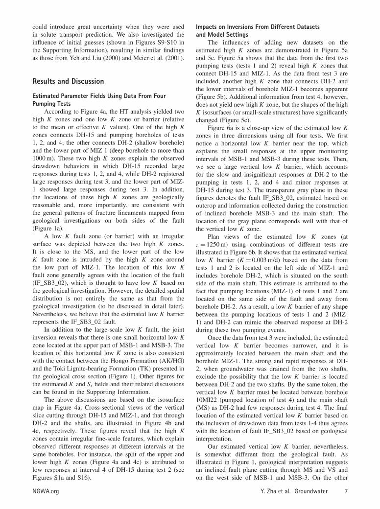
According to Figure 4a, the HT analysis yielded twohigh K zones and one low K zone or barrier (relativeto the mean or effective K values). One of the high Kzones connects DH-15 and pumping boreholes of tests1, 2, and 4; the other connects DH-2 (shallow borehole)and the lower part of MIZ-1 (deep borehole to more than1000 m). These two high K zones explain the observeddrawdown behaviors in which DH-15 recorded largeresponses during tests 1, 2, and 4, while DH-2 registeredlarge responses during test 3, and the lower part of MIZ-1 showed large responses during test 3. In addition,the locations of these high K zones are geologicallyreasonable and, more importantly, are consistent withthe general patterns of fracture lineaments mapped fromgeological investigations on both sides of the fault(Figure 1a).

A low K fault zone (or barrier) with an irregularsurface was depicted between the two high K zones.It is close to the MS, and the lower part of the lowK fault zone is intruded by the high K zone aroundthe low part of MIZ-1. The location of this low Kfault zone generally agrees with the location of the fault(IF_SB3_02), which is thought to have low K based onthe geological investigation. However, the detailed spatialdistribution is not entirely the same as that from thegeological investigation (to be discussed in detail later).Nevertheless, we believe that the estimated low K barrierrepresents the IF_SB3_02 fault.

In addition to the large-scale low K fault, the jointinversion reveals that there is one small horizontal low Kzone located at the upper part of MSB-1 and MSB-3. Thelocation of this horizontal low K zone is also consistentwith the contact between the Hongo Formation (AK/HG)and the Toki Lignite-bearing Formation (TK) presented inthe geological cross section (Figure 1). Other figures forthe estimated K and Ss fields and their related discussionscan be found in the Supporting Information.

The above discussions are based on the isosurfacemap in Figure 4a. Cross-sectional views of the verticalslice cutting through DH-15 and MIZ-1, and that throughDH-2 and the shafts, are illustrated in Figure 4b and4c, respectively. These figures reveal that the high Kzones contain irregular fine-scale features, which explainobserved different responses at different intervals at thesame boreholes. For instance, the split of the upper andlower high K zones (Figure 4a and 4c) is attributed tolow responses at interval 4 of DH-15 during test 2 (seeFigures S1a and S16).

Impacts on Inversions From Different Datasetsand Model Settings

The influences of adding new datasets on theestimated high K zones are demonstrated in Figure 5aand 5c. Figure 5a shows that the data from the first twopumping tests (tests 1 and 2) reveal high K zones thatconnect DH-15 and MIZ-1. As the data from test 3 areincluded, another high K zone that connects DH-2 andthe lower intervals of borehole MIZ-1 becomes apparent(Figure 5b). Additional information from test 4, however,does not yield new high K zone, but the shapes of the highK isosurfaces (or small-scale structures) have significantlychanged (Figure 5c).

Figure 6a is a close-up view of the estimated low Kzones in three dimensions using all four tests. We firstnotice a horizontal low K barrier near the top, whichexplains the small responses at the upper monitoringintervals of MSB-1 and MSB-3 during these tests. Then,we see a large vertical low K barrier, which accountsfor the slow and insignificant responses at DH-2 to thepumping in tests 1, 2, and 4 and minor responses atDH-15 during test 3. The transparent gray plane in thesefigures denotes the fault IF_SB3_02, estimated based onoutcrop and information collected during the constructionof inclined borehole MSB-3 and the main shaft. Thelocation of the gray plane corresponds well with that ofthe vertical low K zone.

Plan views of the estimated low K zones (atz = 1250 m) using combinations of different tests areillustrated in Figure 6b. It shows that the estimated verticallow K barrier (K = 0.003 m/d) based on the data fromtests 1 and 2 is located on the left side of MIZ-1 andincludes borehole DH-2, which is situated on the southside of the main shaft. This estimate is attributed to thefact that pumping locations (MIZ-1) of tests 1 and 2 arelocated on the same side of the fault and away fromborehole DH-2. As a result, a low K barrier of any shapebetween the pumping locations of tests 1 and 2 (MIZ-1) and DH-2 can mimic the observed response at DH-2during these two pumping events.

Once the data from test 3 were included, the estimatedvertical low K barrier becomes narrower, and it isapproximately located between the main shaft and theborehole MIZ-1. The strong and rapid responses at DH-2, when groundwater was drained from the two shafts,exclude the possibility that the low K barrier is locatedbetween DH-2 and the two shafts. By the same token, thevertical low K barrier must be located between borehole10MI22 (pumped location of test 4) and the main shaft(MS) as DH-2 had few responses during test 4. The finallocation of the estimated vertical low K barrier based onthe inclusion of drawdown data from tests 1-4 thus agreeswith the location of fault IF_SB3_02 based on geologicalinterpretation.

Our estimated vertical low K barrier, nevertheless,is somewhat different from the geological fault. Asillustrated in Figure 1, geological interpretation suggestsan inclined fault plane cutting through MS and VS andon the west side of MSB-1 and MSB-3. On the other


DH-15

MSB-3

Test 2

MIZ-1

MSB-1

Test 1

X (m)

Z(m

)

0 500 1000 1500 20000

700

1400

K (m/d)

5.30E+002.04E+007.88E-013.04E-011.17E-014.52E-021.74E-026.72E-032.59E-031.00E-03

(b) Slice across DH-15 and MIZ-1

4

10

1

10

5

4

1

MIZ-1

Test 3

DH-2

X (m)

Z (m

)

0 500 1000 1500 20000

700

1400

K (m/d)

5.30E+002.04E+007.88E-013.04E-011.17E-014.52E-021.74E-026.72E-032.59E-031.00E-03

(c) Slice across DH-2 and the shafts

10

6

1

312

1

Figure 4. The transient inversion results (K tomogram) using data from tests 1, 2, 3, and 4, with (a) highlighted isosurfacesof K = 0.06 m/d (high K zone) and K = 0.003 m/d (low K zone), (b) slice cutting through DH-15 and MIZ-1, and (c) slicethrough DH-2 and MIZ-1. The cubes in (a) mark the locations of the pumping boreholes in tests 1, 2, and 4. The circles arethe observation intervals numbered from top to bottom.

hand, the estimated vertical low K barrier using all theavailable data is highly irregular in shape and inclined,intercepting the main shaft, and running through the gapbetween MSB-1 and MSB-3. More importantly, our HTanalysis shows that this low K fault becomes thinnerwhere the additional boreholes (05ME06, 07MI08, and07MI09) are located.

Furthermore, responses at closely spaced boreholes(05ME06, 07MI08, and 07MI09) at test 4 (see Figure S3)allow mapping small-scale features of the heterogeneity.For instance, an opening (i.e., a high K zone) is found inthe middle of the vertical low K barrier. This estimated“hole” is responsible for the observed rapid and significantresponses observed in borehole 07MI08 (see Figure 5a),located at the west side of the low K fault, and whenthe water was pumping from 10MI22, located at theeast side of the low K fault. Thus, it is probable that07MI08 is connected to the pumped interval in 10MI22of test 4 through small-scale fractures across the low Kfault. This finding suggests that our HT test and analysisyield additional information about the fault, which is notavailable through the geological investigation.

The uncertainty maps of the estimates using differentsubsets of data are also presented in Figures S13-S14.These figures show that the uncertainties of K and S s are

reduced at the regions where new pumping locations orobservation boreholes are located.

Overall, our study shows that the connectivitybetween any two locations on either side of the fault(low permeable fault) can be substantiated only if thepumping tests are conducted on that side of the fault. Forexample, the estimated hydraulic properties on the westside of the fault remain ambiguous when only pumpingtests 1 and 2 (at the east side) are considered, eventhough there are observation boreholes on both sidesof fault. That is, if pumped locations are only locatedat one side of the barrier, signals are likely hinderedby the barrier, and the responses will be very weak.Thus, we suggest that the pumping wells and observationboreholes should be installed on both sides of the faultbased on geological and geophysical information. Thedistances between observation locations would determinethe resolution of heterogeneity estimates, as concludedby Yeh and Liu (2000). This result suggests that priorgeological or geophysical information is important to HTsurvey design (i.e., where the pumping and observationwells should be). Such that more detailed mapping offractures and faults can be obtained.

The impacts on the inversions from two differentmodel settings (the domains, meshes, and boundary


Fig

ure

5.K

(m/d

)to

mog

ram

sob

tain

edfr

omth

ein

vers

ion

ofda

tafr

om(a

)te

sts

1an

d2,

(b)

test

s1-

3,an

d(c

)te

sts

1-4.

Isos

urfa

ceK

=0.

06m

/dhi

ghlig

hts

the

high

Kzo

nes.

The

cube

sm

ark

the

loca

tion

sof

the

pum

ping

bore

hole

sin

test

s1,

2,an

d4.

The

circ

les

deno

teth

elo

cati

ons

ofth

eob

serv

atio

nin

terv

als.


X (m)

Y (m

)

600 800 1000 1200 1400 1600

480

640

800

960

1120

1280

VS

DH-2DH-15

NMSB-1

IF_SB3_02

MSB-3

MSTest 3

MIZ-1 (tests 1 and 2)

(2)(3)

(3) Using data from tests 1-4

(1)



10MI22 (test 4)

(b)

Figure 6. (a) Isosurface K = 0.003 m/d (highlighting the lowK zone) obtained from the inversion of data from tests 1-4.The possible location of fault IF_SB3_02 is also presented.(b) The plan view (z = 1250 m) of the derived locations ofthe fault (low K zone with K = 0.003 m/d) using differentdatasets and the geological location of the fault. Green faultis from the estimation using tests 1 and 2; pink fault is fromthe result using tests 1, 2, and 3; red fault is from the resultusing tests 1, 2, 3, and 4.

conditions) used here and in Illman et al. (2009) areanalyzed and presented in Figures S11-S12. We brieflymention here that the boundary conditions used in thisstudy are more reasonable than those in Illman et al.(2009) as they allow us to reveal the low permeable layernear the top boundary based on geological information(Figure 1b). Moreover, the larger domain used here ishelpful to minimize the boundary effect and suspicioushigh K values in Illman et al. (2009).

ConclusionsIllman et al. (2009) showed that HT is a promising

tool to characterize fault/fractured zones with only fewboreholes and two pumping tests. However, their pumpingtests were conducted on the east side of a geologicallymapped flow barrier (a fault zone). As a result, mostfeatures revealed by HT are limited to the east side,and the location of the barrier is uncertain, although itroughly agrees with that from geological investigation.Our analysis demonstrates that inclusion of new datasetsfrom pumping test 3, which was conducted on the westside of the flow barrier, are crucial to map the correctlocation and depict irregular shape of the barrier and thefracture zone on the west side of the fault. Moreover,the additional data from test 4, close to the barrierilluminate, detailed the shape of the flow barrier andrevealed some presence of preferential flow paths crossthe flow barrier (Figure 6b). These results unambiguouslystress the importance of consideration of prior geologicalinformation (fault zone) during the design of HT surveys,such that important non-redundant information can becollected to improve the resolution of HT estimates,corroborating the results from Yeh and Liu (2000); Wuet al. (2005); Illman et al. (2007); Huang et al. (2011);Berg and Illman (2011, 2013, 2015); Sun et al. (2013);Mao et al. (2013); and Yeh et al. (2014).

Our results also indicate that the inverse modeldomain, boundary conditions, and geostatistical priorinformation for inversion have some impacts on theestimates, which were not investigated in the study byIllman et al. (2009). Instead of assigning a constant headboundary at the top, as done by Illman et al. (2009), ouruse of lateral constant head boundary leads to geologicallyconsistent results, confirming the suggestion by Sun et al.(2013) based on synthetic examples. A larger domain wasproven useful to avoid suspicious boundary effect in theinversion. Furthermore, our analysis show that inversionsbased on different geostatistical prior information shareda common large-scale pattern but differed from each otherin detailed shapes.

Despite the successful application of HT at the MIUsite, it should be recognized that due to the highly discretenature of fractures and faults, it is difficult to map theirdetailed distributions with a limited number of wells.Collecting more non-redundant information is necessaryto increase the resolution (Bohling and Butler, 2010).Lastly, we concur with Bense et al. (2013) that synergisticefforts are required to gain a more integrated andcomprehensive understanding of fault zone hydrogeology.The uncertainty maps obtained in this study can be usedto guide the design of additional HT, geological, andgeophysical surveys.

AcknowledgmentsThis research was supported in part by the NSF EAR

grant 1014594 and in part by the Strategic Environmen-tal Research and Development Program (SERDP) under


grant ER-1365. Additional support for the project wasprovided to Walter A. Illman by the Natural Resourcesand Engineering Council of Canada (NSERC) through theDiscovery grant. The first author acknowledges the sup-port from National Natural Science Foundation of China(No. 51409192). J.-C. Wen would like to acknowledge theresearch support from NSC 101-2221-E-224-050, NSC102-2221-E-224-050, MOST 103-2221-E-224-054, andMOST 104-2221-E-224-039 by the Minister of Scienceand Technology, Taiwan. T.-C.J. Yeh also acknowledgesthe Outstanding Overseas Professorship award throughJilin University by the Department of Education, China.We thank the three anonymous reviewers for their instruc-tive and elaborate comments.

Authors’ NoteThe authors does not have any conflicts of interest or

financial disclosures to report.

Supporting InformationAdditional Supporting Information may be found in theonline version of this article:

Table S1. The computational cost for SimSLE periteration.Appendix S1. Successive Linear Estimator algorithm.Appendix S2. Drawdown responses.Appendix S3. Computational cost of inverse modeling.Appendix S4. Calibration and error issue.Appendix S5. Estimated K and Ss from the joint inversionof the four tests.Appendix S6. Influences of correlation functions.Appendix S7. Influences of model settings.Appendix S8. Uncertainty estimates.Appendix S9. Detailed drawdown-time plots.Figure S1. The drawdown responses during test 2 in asimilar manner as those from tests 1 and 3 presented inthe manuscript.Figure S2. The drawdown responses during test 4 in asimilar manner as those from tests 1 and 3 presented inthe manuscript.Figure S3. The drawdown responses during test 4 withadditional observation wells (05ME06, 07MI08, 07MI09)in a similar manner as those from tests 1 and 3 presentedin the manuscript.Figure S4. The numerical domain and mesh.Figure S5. The calibration map of the joint inversion forthe four tests.Figure S6. Displays the head calibration error and spatialvariances of estimated K and Ss as functions of iterationsduring inversions.Figure S7. The transient inversion results (K estimates)based on the four tests.Figure S8. The transient inversion results (Ss estimates)based on the four tests.Figure S9. The inverse K estimates using large correlationscales (100 m, 100 m and 50 m, respectively).

Figure S10. The inverse K results using the correlationfunction based on the information of the fault orientation.Figure S11. The inverse results (K estimates) using tests1 and 2 with different boundary conditions.Figure S12. The inverse results (Ss estimates) using tests1 and 2 with different boundary conditions.Figures S13. The uncertainty maps of the K estimatesusing different pumping tests.Figure S14. The uncertainty maps of the Ss estimatesusing different pumping tests.Figure S15. Drawdown-time plots for different intervalsof different observation boreholes induced by test 1.Figure S16. Drawdown-time plots for different intervalsof different observation boreholes induced by test 2.Figure S17. Drawdown-time plots for different intervalsof different observation boreholes induced by test 3.Figure S18. Drawdown-time plots for different intervalsof different observation boreholes induced by test 4.

ReferencesBense, V.F., T. Gleeson, S.E. Loveless, O. Bour, and J. Scibek.

2013. Fault zone hydrogeology. Earth-Science Review 127:171–192. DOI:10.1016/j.earscirev.2013.09.008.

Berg, S.J., and W.A. Illman. 2015. Comparison of hydraulictomography with traditional methods at a highlyheterogeneous site. Groundwater 53, no. 1: 71–89.DOI:10.1111/gwat.12159.

Berg, S.J., and W.A. Illman. 2013. Field study of subsurfaceheterogeneity with steady state hydraulic tomography.Groundwater 51, no. 1: 29–40. DOI:10.1111/j.1745-6584.2012.00914.x.

Berg, S.J., and W.A. Illman. 2011. Three-dimensional transienthydraulic tomography in a highly heterogeneous glacioflu-vial aquifer-aquitard system. Water Resources Research 47:W10507. DOI:10.1029/2011WR010616.

Bohling, G., and J. Butler. 2010. Inherent limitations ofhydraulic tomography. Ground Water 48, no. 6: 809–824.DOI:10.1111/j.1745-6584.2010.00757.x.

Brauchler, R., R. Liedl, and P. Dietrich. 2003. A travel timebased hydraulic tomographic approach. Water ResourcesResearch 39, no. 12: 1370. DOI:10.1029/2003WR002262.

Cardiff, M., W. Barrash, and P. Kitanidis. 2013. Hydraulic con-ductivity imaging from 3-D transient hydraulic tomographyat several pumping/observation densities. Water ResourcesResearch 49, no. 11: 7311–7326. DOI:10.1002/wrcr.20519.

Day-Lewis, F.D., J.W. Lane, and S.M. Gorelick. 2006. Com-bined interpretation of radar, hydraulic, and tracer data froma fractured-rock aquifer near Mirror Lake, New Hamp-shire, USA. Hydrogeology Journal 14, no. 1–2: 1–14.DOI:10.1007/s10040-004-0372-y.

Day-Lewis, F.D., J.W.L. Jr., J.M. Harris, and S.M. Gore-lick. 2003. Time-lapse imaging of saline-tracer trans-port in fractured rock using difference-attenuation radartomography. Water Resources Research 39, no. 10: 1290.DOI:10.1029/2002WR001722.

Day-Lewis, F.D., P.A. Hsieh, and S.M. Gorelick. 2000. Iden-tifying fracture-zone geometry using simulated annealingand hydraulic-connection data. Water Resources Research36, no. 7: 1707. DOI:10.1029/2000WR900073.

Hao, Y., T.-C.J. Yeh, J. Xiang, W.A. Illman, K. Ando, K.-C. Hsu, and C.-H. Lee. 2008. Hydraulic tomography fordetecting fracture zone connectivity. Ground Water 46, no.2: 183–192. DOI:10.1111/j.1745-6584.2007.00388.x.

Hsieh, P.A., A.M. Shapiro, and C.R. Tiedeman. 1999. Computersimulation of fluid flow in fractured rocks at the mirror


lake FSE well field, in U.S. Geological Survey ToxicSubstances Hydrology Program—Proceedings of theTechnical Meeting , vol. 3, ed. D.W. Morganwalp andH.T. Buxton, 777–781. Subsurface contamination frompoint sources. U.S. Geological Survey Water-ResourcesInvestigations Report 99-4018C, Charleston SouthCarolina.

Hsieh, P.A., S.P. Neuman, G.K. Stiles, and E.S. Simpson. 1985.Field determination of the three-dimensional hydraulic con-ductivity tensor of anisotropic media 2. Methodology andapplication to fractured rocks. Water Resources Research21, no. 11: 1667–1676. DOI:10.1029/WR021i011p01667.

Huang, S.-Y., J.-C. Wen, T.-C.J. Yeh, W. Lu, H.-L. Juan, C.-M.Tseng, J.-H. Lee, and K.-C. Chang. 2011. Robustness ofjoint interpretation of sequential pumping tests: Numericaland field experiments. Water Resources Research 47, no.10: W10530. DOI:10.1029/2011WR010698.

Illman, W.A. 2014. Hydraulic tomography offers improvedimaging of heterogeneity in fractured rocks. Groundwater52, no. 5: 659–684. DOI:10.1111/gwat.12119.

Illman, W.A., X. Liu, S. Takeuchi, T.-C.C.J. Yeh, K. Ando,and H. Saegusa. 2009. Hydraulic tomography in fracturedgranite: Mizunami underground research site, Japan. WaterResources Research 45, no. 1: W01406. DOI:10.1029/2007WR006715.

Illman, W.A., X. Liu, and A. Craig. 2007. Steady-statehydraulic tomography in a laboratory aquifer with deter-ministic heterogeneity: Multi-method and multiscale val-idation of hydraulic conductivity tomograms. Journalof Hydrology 341, no. 3–4: 222–234. DOI:10.1016/j.jhydrol.2007.05.011.

Japan Atomic Energy Agency. 2010. Master Plan of the Mizu-nami Underground Research Laboratory Project, JAEA-Review 010–016.

Lavenue, M., and G. de Marsily. 2001. Three-dimensionalinterference test interpretation in a fractured aquifer usingthe Pilot Point Inverse Method. Water Resources Research37, no. 11: 2659–2675.

Liu, S., T.-C.J. Yeh, and R. Gardiner. 2002. Effective-ness of hydraulic tomography: Sandbox experiments.Water Resources Research 38, no. 4: 5–1–5–9.DOI:10.1029/2001WR000338.

Mao, D., T.-C.J. Yeh, L. Wan, J.-C. Wen, W. Lu, C.-H. Lee, andK.-C. Hsu. 2013. Cross-correlation analysis and informationcontent of observed heads during pumping in unconfinedaquifers. Water Resources Research 49, no. 4: 1782–1796.DOI:10.1002/wrcr.20066.

Meier, P., A. Medina, and J. Carrera. 2001. Geostatistical inver-sion of cross-hole pumping tests for identifying preferentialflow channels within a shear zone. Groundwater 39, no. I:10–17. DOI:10.1111/j.1745-6584.2001.tb00346.x.

Ni, C.-F., and T.-C.J. Yeh. 2008. Stochastic inversion ofpneumatic cross-hole tests and barometric pressurefluctuations in heterogeneous unsaturated formations.Advances in Water Resources 31, no. 12: 1708–1718.DOI:10.1016/j.advwatres.2008.08.007.

Niwa, M., and R. Takeuchi. 2012. Groundwater pressure changesin Central Japan induced by the 2011 off the Pacific coastof Tohoku Earthquake. Geochemistry, Geophysics, Geosys-tems 13, no. 5: Q05020. DOI:10.1029/2012GC004052.

Saegusa, H., and T. Matsuoka. 2011. Final report on thesurface-based investigation phase (phase 1) at the MizunamiUnderground Research Laboratory project, JAEA-Research2010-067 Ibaraki, Japan.

Sharmeen, R., W.A. Illman, S.J. Berg, T.-C.J. Yeh, Y.-J. Park,E.A. Sudicky, and K. Ando. 2012. Transient hydraulictomography in a fractured dolostone: Laboratory rockblock experiments. Water Resources Research 48, no. 10:W10532. DOI:10.1029/2012WR012216.

Sun, R., T.-C.J. Yeh, D. Mao, M. Jin, W. Lu, and Y. Hao. 2013.A temporal sampling strategy for hydraulic tomographyanalysis. Water Resources Research 49, no. 7: 3881–3896.DOI:10.1002/wrcr.20337.

Tiedeman, C.R., P.J. Lacombe, and D.J. Goode. 2010. Multiplewell-shutdown tests and site-scale flow simulation infractured rocks. Ground Water 48, no. 3: 401–415.DOI:10.1111/j.1745-6584.2009.00651.x.

Tsoflias, G.P., T. Halihan, and J.M. Sharp. 2001. Monitoringpumping test response in a fractured aquifer using ground-penetrating radar of monitoring. Water Resources Research37, no. 5: 1221–1229.

Vesselinov, V.V., S.P. Neuman, and W.A. Illman. 2001.Three-dimensional numerical inversion of pneumatic cross-hole tests in unsaturated fractured tuff 2. Equivalentparameters, high-resolution stochastic imaging and scaleeffects. Water Resources Research 37, no. 12: 3019–3041.DOI:10.1029/2000WR000135.

Wu, C.-M., T.-C.J. Yeh, J. Zhu, T.H. Lee, N.-S. Hsu, C.-H. Chen,and A.F. Sancho. 2005. Traditional analysis of aquifer tests:Comparing apples to oranges? Water Resources Research41, no. 9: W09402. DOI:10.1029/2004WR003717.

Xiang, J., T.-C.J. Yeh, C.-H. Lee, K.-C. Hsu, and J.-C.Wen. 2009. A simultaneous successive linear estimatorand a guide for hydraulic tomography analysis. WaterResources Research 45, no. 2: W02432. DOI:10.1029/2008WR007180.

Yeh, T.-C.J., D. Mao, Y. Zha, K.-C.C. Hsu, C.-H.H. Lee, J.-C.C. Wen, W. Lu, and J. Yang. 2014. Why hydraulictomography works? Ground Water 52, no. 2: 168–172.DOI:10.1111/gwat.12129.

Yeh, T.-C.J., and C.-H. Lee. 2007. Time to change the waywe collect and analyze data for aquifer characteriza-tion. Ground Water 45, no. 2: 116–118. DOI:10.1111/j.1745–6584.2006.00292.x.

Yeh, T.-C.J., and S. Liu. 2000. Hydraulic tomography:Development of a new aquifer test method. WaterResources Research 36, no. 8: 2095–2105. DOI:10.1029/2000WR900114.

Zhu, J., and T. Yeh. 2005. Characterization of aquifer het-erogeneity using transient hydraulic tomography. WaterResources Research 41, no. 7: 1–10. DOI:10.1029/2004WR003790.


an application of hydraulic tomography to a large-scale fractured

Documents