an analysis of live streaming workloads on the internet · an analysis of live streaming workloads...
TRANSCRIPT
An Analysis of Live Streaming Workloads on the Internet�
Kunwadee Sripanidkulchai, Bruce Maggs,�
and Hui Zhang
Carnegie Mellon University
ABSTRACTIn this paper, we study the live streaming workload from a largecontent delivery network. Our data, collected over a 3 month pe-riod, contains over 70 million requests for 5,000 distinct URLs fromclients in over 200 countries. To our knowledge, this is the most ex-tensive data of live streaming on the Internet that has been studiedto date. Our contributions are two-fold. First, we present a macro-scopic analysis of the workload, characterizing popularity, arrivalprocess, session duration, and transport protocol use. Our resultsshow that popularity follows a 2-mode Zipf distribution, session in-terarrivals within small time-windows are exponential, session du-rations are heavy-tailed, and that UDP is far from having universalreach on the Internet. Second, we cover two additional character-istics that are more specific to the nature of live streaming applica-tions: the diversity of clients in comparison to traditional broadcastmedia like radio and TV, and the phenomena that many clients reg-ularly join recurring events. We find that Internet streaming doesreach a wide audience, often spanning hundreds of AS domains andtens of countries. More interesting is that small streams also havea diverse audience. We also find that recurring users often havelifetimes of at least as long as one-third of the days in the event.
Categories and Subject DescriptorsC.2 [Computer-Communication Networks]: Distributed Systems
General TermsMeasurement�This research was sponsored by DARPA under contract num-
ber F30602-99-1-0518, US Army Research Office under awardDAAD19-02-1-0389, and by NSF under grant numbers CareerAward NCR-9624979 ANI-9730105, ITR Award ANI-0085920,ANI-9814929, ANI-0331653,and CCR-0205523. Additional sup-port was provided by Intel. Views and conclusions contained inthis document are those of the authors and should not be interpretedas representing the official policies, either expressed or implied, ofDARPA, US ARO, NSF, Intel, or the U.S. government.�Bruce Maggs is also with Akamai Technologies.
Permission to make digital or hard copies of all or part of this work forpersonal or classroom use is granted without fee provided that copies arenot made or distributed for profit or commercial advantage and that copiesbear this notice and the full citation on the first page. To copy otherwise, torepublish, to post on servers or to redistribute to lists, requires prior specificpermission and/or a fee.IMC’04, October 25–27, 2004, Taormina, Sicily, Italy.Copyright 2004 ACM 1-58113-821-0/04/0010 ...$5.00.
KeywordsLive streaming, content delivery networks
1. INTRODUCTIONWhile live streaming is still in its early stages on the Internet, it
is likely to become an important traffic class because of both appli-cation pull and technology push. From an application’s perspective,the Internet provides a new medium for live streaming that has sev-eral advantages over traditional media. With traditional media suchas radio, TV, and satellite, there are a limited number of channels.Also, radio and TV usually have limited reach. These media arevery expensive and are accessible to only a few content publishers.In contrast, hundreds of thousands of sessions can be conducted si-multaneously over the Internet at any given time. The number ofparticipants in each session is determined by the application ratherthan the network. Therefore, the Internet provides an attractive al-ternative to reach global audiences ranging from small, medium tolarge sizes. As people become more mobile, traveling and workingaround the globe, the demand for “connecting back to home” bylistening or watching content that has traditionally been local willincrease. From a technology perspective, as broadband access be-comes more ubiquitous and multimedia devices become an integralpart of computers, PDAs, and cell phones, the technology barrier tolive streaming will disappear.
While there are extensive studies of Web [11, 9, 15, 2, 5] andon-demand streaming [24, 6, 1] workloads on the Internet, there area few live streaming [23]. Understanding live streaming workloadswill provide insight into how the broadcast medium is being usedand how it may be used in the future. Such insight is useful forsystem design, evaluation, planning, and management [4, 19, 22].
In this paper, we analyze the live streaming workloads fromAkamai Technologies, the largest content distribution network onthe Internet. Our data is collected over a 3-month period, with morethan 70 million requests for 5,000 distinct URLs. Our analysis cov-ers some of the common characteristics typically used to describeworkloads, such as popularity, session arrivals, session duration,and transport protocol usage. In addition, we cover two additionalcharacteristics that are more specific to the nature of live stream-ing: the diversity of the client population in comparison to tradi-tional broadcast media like radio and TV, and the recurring natureof clients. Overall our analysis is macroscopic, discussing commontrends observed across many URLs.
We summarize the findings in our paper below:� Audio traffic is more popular than video traffic on this CDN.
Only 1% of the requests are for video streams. And only 7%of streams are video streams.� The popularity of live streaming events follows a Zipf-likedistribution with 2 distinct modes. This is in stark contrast to

popularity of Web objects, but consistent with previous find-ings for on-demand streaming.� Non-stop streams have strong time-of-day and time zone cor-related behavior. Short streams have negligible time-of-daybehavior. Furthermore, a surprisingly large number of streamsexhibit flash crowd behavior. We find that 50% of all largestreams, non-stop and short durations, have flash crowds.� Session duration distributions are heavy-tailed. The tails have3 distinct shapes corresponding to 3 types of streams: non-stop with fresh content, non-stop with cyclic content, andshort streams.� Almost half of the AS domains seen in our logs tend to useTCP as the dominant transport protocol. Such characteristicscould perhaps be caused by the presence of network addresstranslators (NATs) and firewalls that disallow the use of UDP.� Client lifetime is bimodal for recurring events. Half of thenew clients who tune in to a stream will tune in for only oneday. For the remaining half, their average lifetime is at leastas long as one-third of the days in the event.� The diversity of clients accessing live streams on the Internetis much wider than traditional broadcast media such as radioand local TV. Almost all large streams reach 13 or more dif-ferent time zones, 10 or more different countries, and 200or more different AS domains. The majority of the smallstreams reach 11 or more different time zones, 10 or moredifferent countries, and 100 or more different AS domains.
In Section 2, we discuss our methodology and provide a high-level characterization of the workload. In Sections 3, 4, and 5,we analyze the popularity of streaming events, classify events intotypes, and characterize the session arrivals and durations. We dis-cuss the use of transport protocols in Section 6. In Section 7, wepresent our analysis on the diversity of the clients tuning in to thestreams. Section 8 discusses the client birthrate and the lifetime ofclients. We discuss related work in Section 9 and summarize ourfindings in Section 10.
2. METHODOLOGYIn this section, we discuss the methodology we use to collect
and process logs.
2.1 Data Source and Log CollectionThe logs used in our study are collected from thousands of
streaming servers belonging to Akamai Technologies which oper-ates a large content delivery network. Akamai’s streaming networkis a static overlay composed of (i) edge nodes that are located atthe edge of the network, close to clients, and (ii) intermediate nodesthat take streams from the original content publisher and split andreplicate them to the edge nodes. The logs that we use in this studyare from the edge nodes that directly serve client requests.
Our log collection process involves pulling logs from the pro-duction network into our log collection server. Each edge nodedumps hourly logs of all content that it has served into a centralizedrepository. The repository consists of a large number of machines inone physical location, and is part of the Akamai production network.Each machine in the repository runs NFS and can mount any of theother machines’ disk drives. To collect the logs for our study, wetapped into one of these machines and mounted all the relevant diskdrives. All hourly logs from all edge servers were then copied fromthe repository into our log collection server, which is separate fromthe Akamai production network. Note that an edge server generallyserves content belonging to multiple content publishers/URLs. To
facilitate our analysis, we sort and extract log entries from the thou-sands of edge servers into URL-based files at 24-hour granularities.
2.2 DefinitionsClients
A client is defined to be a unique user, identified by either its IPaddress or player ID. For most of the analysis in this paper, we useIP addresses unless otherwise stated.Events vs. Streams
We make a distinction between events and streams. An eventcorresponds to a URL. An event can happen for short durations (forexample, a 2-hour talk show), or non-stop across multiple days (forexample, a 24-hour a day, 7-days a week radio station). On theother hand, a stream is defined as a 24-hour chunk of the event. Ifan entire event lasts less than a day, then a stream is the equivalentof an event. All analysis in the following sections are conductedeither at the granularity of streams or events, as stated.
2.3 Log Format and ProcessingEach entry in the log corresponds to a session, or a request made
by a client to an edge server. The following fields extracted fromeach entry are used in our study.
� User identification: IP address and player ID� Requested object: URL� Time-stamps: session start time and session duration at thegranularity of seconds� Performance statistics: average received bandwidth for entireduration
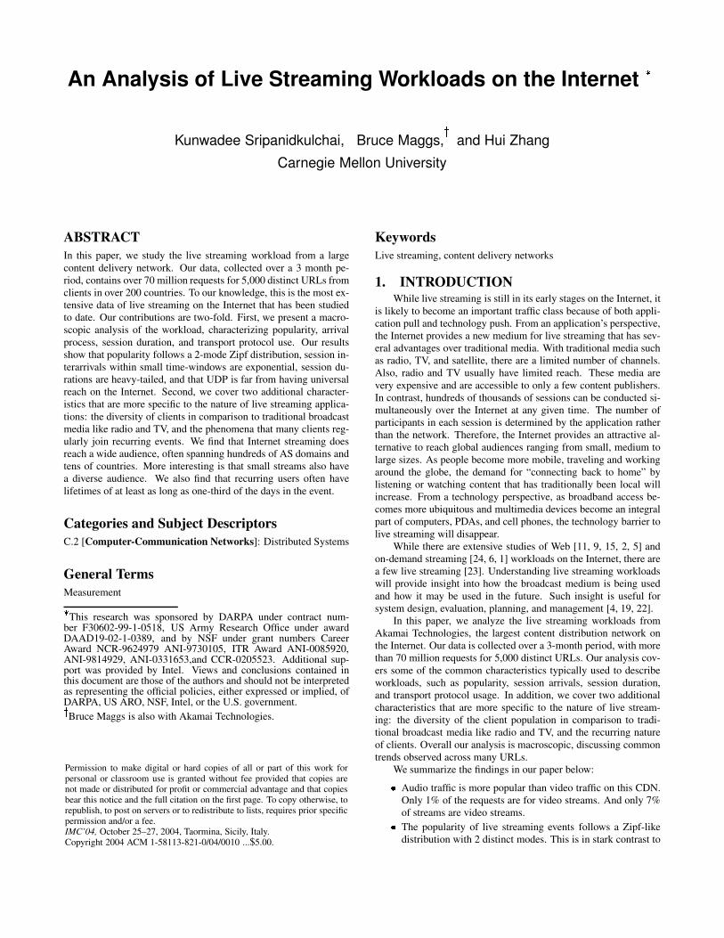
2.4 High-Level CharacteristicsThe logs were collected over a 3-month period from October
2003 to January 2004. The daily statistics for live streaming trafficduring that period are depicted in Figure 1. The traffic consists ofthree of the most popular streaming media formats, Apple Quick-Time, Microsoft Windows Media, and Real. As Figure 1(a) shows,there were typically 900-1,000 distinct streams on most days. How-ever, there was a sharp drop in early December and a drop againin mid-December to January (denoted by the vertical lines). This isbecause we had a problem with our log collection infrastructure anddid not collect logs for one of formats on those days. Figure 1(b)depicts the number of requests for live streams, which varies from600,000 on weekends to 1 million on weekdays. Again, the dropin requests from mid-December onwards is due to the missing logs.The total number of distinct client IP addresses served is roughly175,000 per day, as depicted in Figure 1(c). The patterns mimic thetotal number of requests. On average a distinct IP address issues 4requests.
2.5 Audio vs. Video Event IdentificationThe logs do not specify content type information. In order to
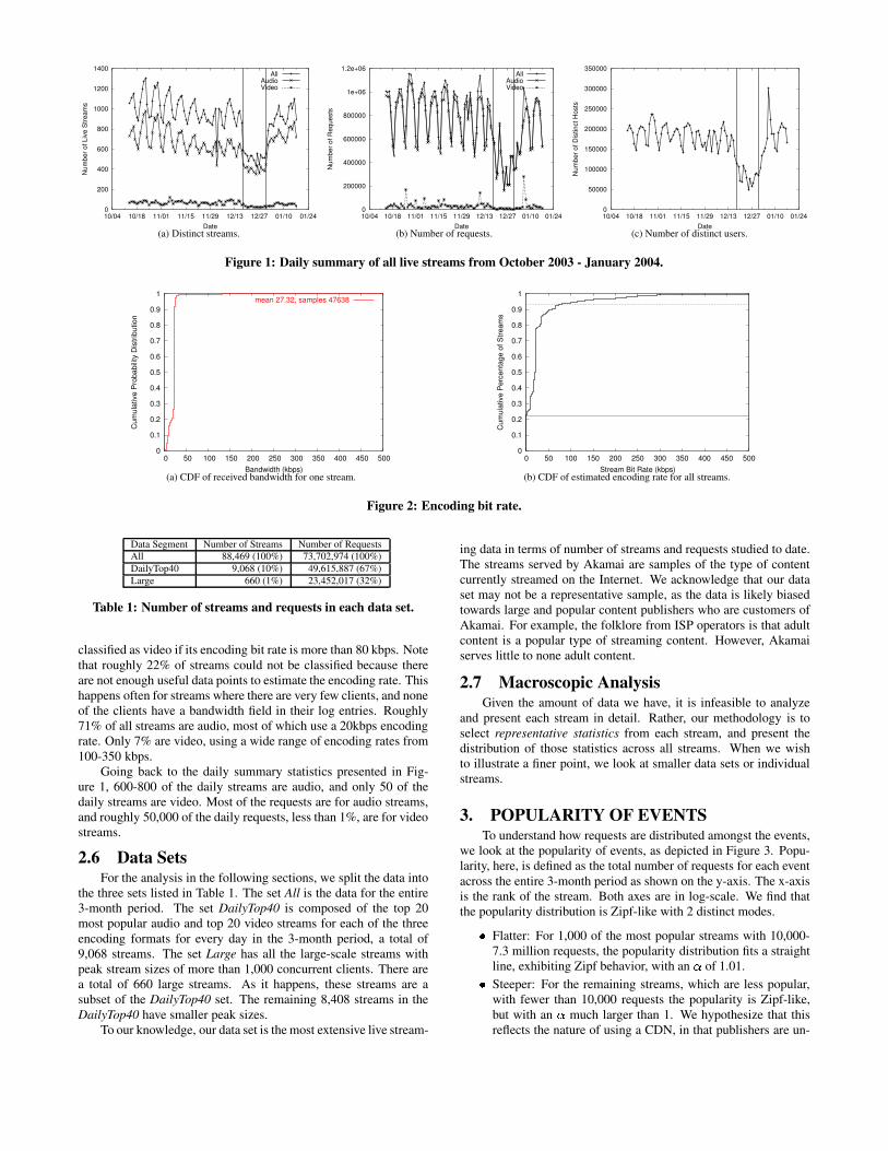
identify whether a stream corresponds to an audio or video stream,we look at the encoding bit rate. The encoding rate is estimatedfrom the logs using the median of the receiving bandwidth thatclients report back to the server across all clients receiving the samestream. We use the median (as opposed to the mean) as it is morerobust to large errors which may bias the estimate. Figure 2(a) de-picts the cumulative distribution of received bandwidth for an audiostream. Note that most hosts are receiving at 20 kbps, and the me-dian is at 20 kbps. The mean, however, is at 27 kbps because therewere a few log entries that erroneously reported bandwidth valuesof up to Mbps, biasing the mean.
Figure 2(b) depicts the cumulative distribution of estimated en-coding rate for all streams across the 3-month period. A stream is
0
200
400
600
800
1000
1200
1400
10/04 10/18 11/01 11/15 11/29 12/13 12/27 01/10 01/24
Num
ber o
f Liv
e S
tream
s
Date
AllAudioVideo
(a) Distinct streams.
0
200000
400000
600000
800000
1e+06
1.2e+06
10/04 10/18 11/01 11/15 11/29 12/13 12/27 01/10 01/24
Num
ber o
f Req
uest
s
Date
AllAudioVideo
(b) Number of requests.
0
50000
100000
150000
200000
250000
300000
350000
10/04 10/18 11/01 11/15 11/29 12/13 12/27 01/10 01/24
Num
ber o
f Dis
tinct
Hos
ts
Date(c) Number of distinct users.
Figure 1: Daily summary of all live streams from October 2003 - January 2004.
0
0.1
0.2
0.3
0.4
0.5
0.6
0.7
0.8
0.9
1
0 50 100 150 200 250 300 350 400 450 500
Cum
ulat
ive
Pro
babi
lity
Dis
tribu
tion
Bandwidth (kbps)
mean 27.32, samples 47638
(a) CDF of received bandwidth for one stream.
0
0.1
0.2
0.3
0.4
0.5
0.6
0.7
0.8
0.9
1
0 50 100 150 200 250 300 350 400 450 500
Cum
ulat
ive
Per
cent
age
of S
tream
s
Stream Bit Rate (kbps)(b) CDF of estimated encoding rate for all streams.
Figure 2: Encoding bit rate.
Data Segment Number of Streams Number of RequestsAll 88,469 (100%) 73,702,974 (100%)DailyTop40 9,068 (10%) 49,615,887 (67%)Large 660 (1%) 23,452,017 (32%)
Table 1: Number of streams and requests in each data set.
classified as video if its encoding bit rate is more than 80 kbps. Notethat roughly 22% of streams could not be classified because thereare not enough useful data points to estimate the encoding rate. Thishappens often for streams where there are very few clients, and noneof the clients have a bandwidth field in their log entries. Roughly71% of all streams are audio, most of which use a 20kbps encodingrate. Only 7% are video, using a wide range of encoding rates from100-350 kbps.
Going back to the daily summary statistics presented in Fig-ure 1, 600-800 of the daily streams are audio, and only 50 of thedaily streams are video. Most of the requests are for audio streams,and roughly 50,000 of the daily requests, less than 1%, are for videostreams.
2.6 Data SetsFor the analysis in the following sections, we split the data into
the three sets listed in Table 1. The set All is the data for the entire3-month period. The set DailyTop40 is composed of the top 20most popular audio and top 20 video streams for each of the threeencoding formats for every day in the 3-month period, a total of9,068 streams. The set Large has all the large-scale streams withpeak stream sizes of more than 1,000 concurrent clients. There area total of 660 large streams. As it happens, these streams are asubset of the DailyTop40 set. The remaining 8,408 streams in theDailyTop40 have smaller peak sizes.
To our knowledge, our data set is the most extensive live stream-
ing data in terms of number of streams and requests studied to date.The streams served by Akamai are samples of the type of contentcurrently streamed on the Internet. We acknowledge that our dataset may not be a representative sample, as the data is likely biasedtowards large and popular content publishers who are customers ofAkamai. For example, the folklore from ISP operators is that adultcontent is a popular type of streaming content. However, Akamaiserves little to none adult content.
2.7 Macroscopic AnalysisGiven the amount of data we have, it is infeasible to analyze
and present each stream in detail. Rather, our methodology is toselect representative statistics from each stream, and present thedistribution of those statistics across all streams. When we wishto illustrate a finer point, we look at smaller data sets or individualstreams.
3. POPULARITY OF EVENTSTo understand how requests are distributed amongst the events,
we look at the popularity of events, as depicted in Figure 3. Popu-larity, here, is defined as the total number of requests for each eventacross the entire 3-month period as shown on the y-axis. The x-axisis the rank of the stream. Both axes are in log-scale. We find thatthe popularity distribution is Zipf-like with 2 distinct modes.
� Flatter: For 1,000 of the most popular streams with 10,000-7.3 million requests, the popularity distribution fits a straightline, exhibiting Zipf behavior, with an � of 1.01.� Steeper: For the remaining streams, which are less popular,with fewer than 10,000 requests the popularity is Zipf-like,but with an � much larger than 1. We hypothesize that thisreflects the nature of using a CDN, in that publishers are un-

1
10
100
1000
10000
100000
1e+06
1e+07
1 10 100 1000 10000
Num
ber o
f Req
uest
s
Event Rank
Three monthsOne day
Figure 3: Popularity of events.
likely to pay a CDN to host unpopular content, as a singleserver hosted by the content publisher may suffice to get thejob done.
To see what the popularity distribution looks like at smallertimescales, we randomly pick one day from our logs, and plot thepopularity distribution of requests that arrived on that one day onthe same scale as the 3-month distribution. As depicted in Figure 3,the one-day distribution looks similar to the 3-month one.
Our findings are in contrast to previously studied popularity dis-tributions for Web objects that report that the popularity is Zipf-likewith only one mode [11, 9, 15, 2, 5]. However, a 2-mode Zipf distri-bution is consistent with studies of on-demand streaming objects [1,6] and multimedia file-sharing workloads [12].
4. CLASSIFICATION OF STREAMSIn this section, we present a scheme for classifying streams
(24-hour chunks of events) into types. We use this classificationthroughout the paper when we wish to show that certain propertiesare related to the type of stream.
4.1 Large vs. SmallThere are several definitions of large streams: total number of
requests (discussed in Section 3), total unique clients, and peak con-current clients. While all three definitions are related, for this paper,we choose the third definition: peak concurrent clients as it is anindicator of how much server capacity needs to be provisioned toaccommodate the stream. Using the definition from Section 2, largestreams have a peak of at least 1,000 concurrent clients. Out of our3-month data set, 660 streams are large. All other streams are small.
4.2 Non-Stop vs. Short DurationsNon-stop streams are streams that are broadcast live every day,
all hours of the day. This is similar to always being “on-the-air” inradio terminology. On the other hand, short duration streams havewell-defined durations typically on the order of a few hours. Anexample of a short-duration stream is a talk show that runs from9am-10am that is broadcast only during that period, and has no traf-fic at any other time during the day. To distinguish between thesetwo stream types we look at the stream duration. However, the logsdo not provide us with any explicit stream duration field. Therefore,we estimate the stream duration using two different methods. Wethen compare the resulting classification to confirm the accuracy ofthe methods.
The first method follows directly from our definition that a non-stop stream is always on 24-hours a day. To capture that prop-erty, we estimate the “stream duration” from the logs. We definethe stream duration as the period of time for which the stream has�������� ��
or more concurrent receivers, where�������� ��
is set at 10.A threshold of 10 is relatively robust at estimating stream durationfor large streams. If a stream duration is roughly 24 hours, then it isa non-stop stream.
Note that this methodology does not work for small streams.For example, consider an unpopular non-stop radio station that hasa sparse audience of 1-2 concurrent clients during the day and noclients at night even though the content is available 24 hours a day.Even with an
� ������ ��of 1, we would estimate the stream duration
to be only during the day, which is incorrect. For correctness, weonly classify large streams.
The cumulative distribution of stream durations for large streamsis depicted in Figure 4(a). The x-axis is the stream duration, and they-axis is the CDF. We find that 76% of streams are non-stop, and theremaining 24% have short durations. We also experimented withother
� ������ ��values and did not find significant differences except
for when the threshold was very low (1 or 2). In such cases, thismethod was susceptible to including “idle time” in the stream du-ration when one or two clients access the URL for a short durationstream before the stream officially started.
The second method examines the slope of the tail of the ses-sion duration distribution, where a session duration is defined as theamount of time a request lasts (how long the client associated withthe request receives data). If a stream’s tail has a steep slope, it is ashort duration stream. See Section 5.2 for a more detailed descrip-tion of this property. Figure 4(b) depicts the cumulative percentageof streams and the slope of the tail. Roughly 20% of streams hada tail slope of -4 or steeper (where steeper means a more negativenumber).
We then compared the streams classified using the two meth-ods against one another and found a good agreement: roughly 92%matched. When the two methods did not agree, it was for streamsthat were short, but had relatively long stream durations (close to 24hours).
We wish to note that in our data set, all video streams wereshort. It is possible that the higher cost of delivering non-stop videocompared to audio is a deterrent for content publishers.
4.3 Recurring vs. One-TimeA recurring stream is defined as one in which the event URL
(say Radio Station X) shows up on multiple days. Recurrence maybe periodic, for example, a daily event. Or, it may follow a pre-determined schedule, for example, a cricket series will often usethe same URL for many of its matches throughout the series. Wefind that 97% of large streams are recurring. Note that all non-stop streams are recurring by definition. However, there are alsorecurring short duration streams, such as daily 2-hour talk shows.About 21% of large streams are these short recurring streams.
4.4 Flash Crowd vs. Smooth ArrivalsDuring a flash crowd, there is a large increase in the number of
people wanting to tune in to the stream. In turn, the arrival rate andtotal number of concurrent clients increase at a rate that is higherthan average. A stream with smooth arrivals, on the other hand, seeseither no change or gradual changes (due to time of day effects).
All short duration streams have flash crowd behavior. Intu-itively, this is because short duration streams take place during aspecific period, for example 2 hours. It is natural for people to wantto start joining and watching the stream from the beginning. In ad-dition, a number of non-stop streams also have flash crowds. We
0
0.1
0.2
0.3
0.4
0.5
0.6
0.7
0.8
0.9
1
0 5 10 15 20 25
Cum
ulat
ive
Per
cent
age
of S
tream
s
Stream Duration (hours)(a) Stream duration.
0
0.1
0.2
0.3
0.4
0.5
0.6
0.7
0.8
0.9
1
-35 -30 -25 -20 -15 -10 -5 0
Cum
ulat
ive
Per
cent
age
of S
tream
s
Tail Slope(b) Tail slope.
Figure 4: Classify streams as non-stop or short.
believe that there are sometimes specific content-related events thathappen for a brief period during the non-stop stream. For example,an invited guest appearance can cause a flash crowd.
To detect whether or not a stream has flash crowd behavior, welook at the stream’s arrival rate over time. We first ran a low-passfilter on the data by looking at “smoothed” arrival rates, averagedover 10-minute windows. Any sudden increase (large slope) in thearrival rate is flagged as flash crowd behavior. We find that setting aminimum threshold at a slope of 3 (a 3-times increase in the arrivalrate compared to the previous window) is reasonable based on visualinspection. About 50% of the large streams are detected as havingflash crowd behavior.
The prominence of flash crowd events in the streams has severalimplications on systems design. While there are a few systems de-signs that consider flash crowds [19], the problem has been largelyignored. Our findings indicate that flash crowds are the norm inlive streaming workloads and systems must be able to cope withsizable changes in the request volume. The system should be ableto support new hosts wanting to connect (in the Akamai network,this requires a DNS-based name resolution to the IP address of aserver) and new hosts connecting to the system (a request packet toa streaming server). Over-engineering, redundancy [4], and mecha-nisms for rejecting requests to prevent the system from melt-downin both the DNS and the streaming infrastructure can help. To ourknowledge, throughout the 3-month data collection period, the Aka-mai network was able to serve the entire request volume presentedto it.
5. SESSION CHARACTERISTICSIn this section, we conduct our analysis on sessions. Recall that
a session is defined at the granularity of a client request, i.e., onerequest is one session. We first look at the session arrival process,and then at the session duration distribution.
5.1 Arrival Process
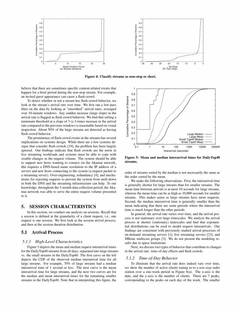
5.1.1 High-Level CharacteristicsFigure 5 depicts the mean and median request interarrival times
for the DailyTop40 streams from all days, separated into large streamsvs. the small streams in the DailyTop40. The first curve on the leftdepicts the CDF of the observed median interarrival time for alllarge streams. For example, 70% of large streams had a medianinterarrival time of 1 second or less. The next curve is the meaninterarrival time for large streams, and the next two curves are forthe median and mean interarrival times for the remaining smallerstreams in the DailyTop40. Note that in interpreting this figure, the
0
0.1
0.2
0.3
0.4
0.5
0.6
0.7
0.8
0.9
1
0.1 1 10 100 1000 10000 100000
Cum
ulat
ive
Per
cent
age
of S
tream
s
Interarrival (seconds)
Large MedianLarge Mean
Small Top40 MedianSmall Top40 Mean
Figure 5: Mean and median interarrival times for DailyTop40streams.
order of streams sorted by the median is not necessarily the same asthe order sorted by the mean.
We make the following observations. First, the interarrival timeis generally shorter for large streams than for smaller streams. Themean time between arrivals is at most 10 seconds for large streams,whereas the mean time can be as high as 10,000 seconds for smallerstreams. This makes sense as large streams have more requests.Second, the median interarrival time is generally smaller than themean indicating that there are some periods where the interarrivaltime is much longer than the other periods.
In general, the arrival rate varies over time, and the arrival pro-cess is not stationary over large timescales. We analyze the arrivalprocess at shorter (stationary) timescales and find that exponen-tial distributions can be used to model request interarrivals. Ourfindings are consistent with previously studied arrival processes ofon-demand streaming servers [1], live streaming servers [23], andMBone multicast groups [3]. We do not present the modeling re-sults due to space limitations.
Next, we discuss two types of behavior that contribute to changesin the arrival rate: time-of-day effects and flash crowds.
5.1.2 Time-of-Day BehaviorTo illustrate that the arrival rate does indeed vary over time,
we show the number of active clients tuning in to a non-stop radiostation over a one-week period in Figure 6(a). The x-axis is thedate, and the y-axis is the number of clients. There are 7 peaks,corresponding to the peaks on each day of the week. The smaller

0
200
400
600
800
1000
1200
10/14 10/15 10/16 10/17 10/18 10/19 10/20 10/21
Num
ber o
f Hos
ts
Date
All UK US PL
(a) Group membership.
0
5
10
15
20
25
30
35
40
14 15 16 17 18 19 20 21
Arriv
al R
ate
(clie
nts/
min
ute)
Date(b) Arrival rate smoothed over 10-minute intervals.
Figure 6: Arrivals for a radio station over a one week period.
peaks correspond to the weekend. The corresponding arrival ratesin number of clients/minute are shown in Figure 6(b). Note thatthe arrivals roughly mirror the weekly and daily trends in the groupmembership pattern. Over the course of a day, the arrival rates varyfrom 5 arrivals/minute to up to 20 arrivals/minute.
To better understand the time-of-day behavior, we break thegroup membership down by country. We map client IP addressesto their geographic location. Figure 6(a) depicts the group member-ship over time for the top 3 participating countries: the UK, the US,and Poland (labelled PL). The daily peaks in the group member-ship are shifted by several hours. The peak for PL occurs roughly2 hours before the peak in UK. And, the peak in the US followsthe UK peak by roughly 4-5 hours. This clearly reflects time-of-day differences as the clients of this one event are scattered acrossmultiple time zones. Interestingly, however, the peaks always occurat around 3-4pm local time. The arrival rates, not shown, are alsoshifted accordingly. When modeling arrival processes, one mustalso consider different arrival rates for clients from different timezones.
5.1.3 Flash CrowdsThis particular stream is interesting in that in addition to the
weekly and daily cyclical trends, there is also some flash crowdbehavior where the arrivals peak as high as 40 arrivals/minute com-pared to the usual 20 arrivals/minute. Flash crowds occurred on 3separate days, on the 15th, 16th and 17th. US clients caused theflash crowds on the 15th and 17th, whereas UK clients caused asmaller flash crowd on the 16th.
Our observations for this particular radio station holds for manyother non-stop streams. For short duration streams, we see lesstime-of-day and time-zone related behavior, as client requests areperhaps driven by the content itself. Perhaps people are willing totune in to a short duration stream at 4am in the morning if the con-tent is meaningful to them. One interesting observation is that all
0
0.1
0.2
0.3
0.4
0.5
0.6
0.7
0.8
0.9
1
0.01 0.1 1 10 100 1000 10000
Cum
ulat
ive
Per
cent
age
of S
tream
s
Session Duration (minutes)
Large MedianLarge Mean
Small Top40 MedianSmall Top40 Mean
Figure 7: Mean and median session duration for DailyTop40streams.
short duration streams exhibit flash crowd behavior, and some non-stop streams such as the one in Figure 6 also exhibit flash crowdbehavior on some days. Overall, we find that 50% of large streamshave flash crowds as reported in Section 4.4.
5.2 Session Duration
5.2.1 High-Level CharacteristicsFigure 7 depicts the mean and median session duration times in
minutes for all the DailyTop40 streams from all days, separated intolarge streams vs. the remaining smaller streams in the DailyTop40.The first two curves on the right correspond to the mean and mediansession durations for large streams, whereas the two curves on theleft correspond to the remaining smaller streams.
As one would expect, large streams have much larger sessiondurations than smaller streams. In terms of statistical measuresof correlation, we find that the correlation coefficient between agroup’s peak size and its median session duration is small at 0.2,but the Spearman’s rank correlation is much stronger at 0.7. Rankcorrelation gives a picture of how the rank of the streams sortedby peak group size agrees with the rank sorted by median sessionduration.
We make two additional observations from Figure 7. First, fora small portion of the streams, the median session duration is ex-tremely small–less than 10 seconds. While we do not know theactual cause of such small session durations, we hypothesize thatsome of it may be caused by “channel surfing.” Such small val-ues can have implications on systems design. The group member-ship for the stream is changing very rapidly. This indicates that theservers should quickly time-out on per-session state (for example,TCP time-outs should be short such that sockets can be freed fornewer connections),and servers should do only a minimal amountof work to set up a session as it will be shut down quickly.
Our second observation is that, for large streams, the sessiondurations are heavy tailed as the observed mean is much larger thanthe median for all sessions. There are a few clients who tune in tothe content for very long periods, whereas most clients only stay formuch shorter periods. The first curve from the right depicts the CDFof the observed mean session duration for all large streams. Forexample, all large streams had a mean session duration larger than30 minutes, and almost all (99.7%) had a mean session duration ofmore than an hour. While the mean is large for most sessions, themedian is much shorter, as depicted by the second curve from the
1e-06
1e-05
0.0001
0.001
0.01
0.1
1
0.01 0.1 1 10 100 1000 10000 100000
Cum
ulat
ive
Per
cent
age
of S
tream
s
Session Duration (minutes)(a) Non-stop streams.
1e-06
1e-05
0.0001
0.001
0.01
0.1
1
0.01 0.1 1 10 100 1000 10000 100000
Cum
ulat
ive
Per
cent
age
of S
tream
s
Session Duration (minutes)(b) Short streams.
Figure 8: Complementary cumulative distribution of session duration for large streams.
right. The median ranges from under 4 minutes to 140 minutes.About 40% of streams had median session durations of shorter than20 minutes.
5.2.2 Tail AnalysisNext, we focus our session duration analysis on the tail of the
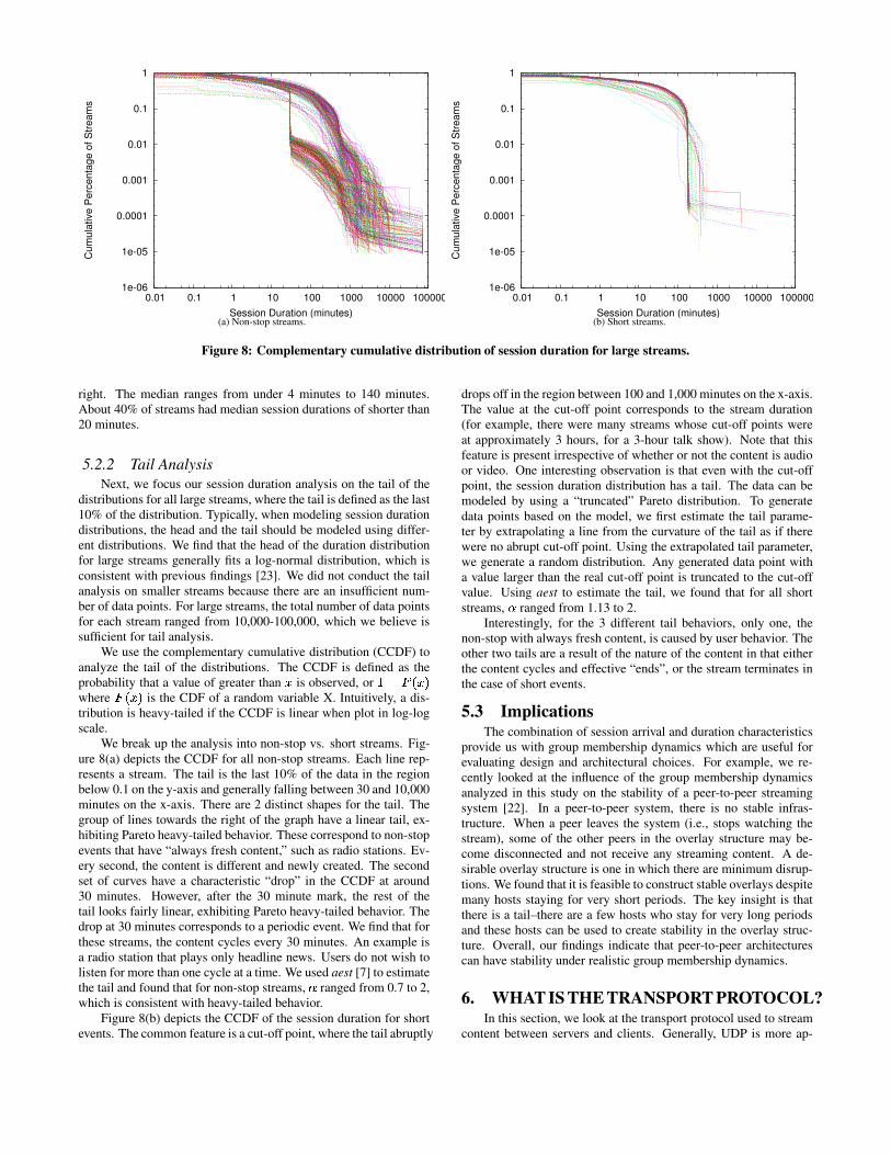
distributions for all large streams, where the tail is defined as the last10% of the distribution. Typically, when modeling session durationdistributions, the head and the tail should be modeled using differ-ent distributions. We find that the head of the duration distributionfor large streams generally fits a log-normal distribution, which isconsistent with previous findings [23]. We did not conduct the tailanalysis on smaller streams because there are an insufficient num-ber of data points. For large streams, the total number of data pointsfor each stream ranged from 10,000-100,000, which we believe issufficient for tail analysis.
We use the complementary cumulative distribution (CCDF) toanalyze the tail of the distributions. The CCDF is defined as theprobability that a value of greater than � is observed, or �����������where ������� is the CDF of a random variable X. Intuitively, a dis-tribution is heavy-tailed if the CCDF is linear when plot in log-logscale.
We break up the analysis into non-stop vs. short streams. Fig-ure 8(a) depicts the CCDF for all non-stop streams. Each line rep-resents a stream. The tail is the last 10% of the data in the regionbelow 0.1 on the y-axis and generally falling between 30 and 10,000minutes on the x-axis. There are 2 distinct shapes for the tail. Thegroup of lines towards the right of the graph have a linear tail, ex-hibiting Pareto heavy-tailed behavior. These correspond to non-stopevents that have “always fresh content,” such as radio stations. Ev-ery second, the content is different and newly created. The secondset of curves have a characteristic “drop” in the CCDF at around30 minutes. However, after the 30 minute mark, the rest of thetail looks fairly linear, exhibiting Pareto heavy-tailed behavior. Thedrop at 30 minutes corresponds to a periodic event. We find that forthese streams, the content cycles every 30 minutes. An example isa radio station that plays only headline news. Users do not wish tolisten for more than one cycle at a time. We used aest [7] to estimatethe tail and found that for non-stop streams, � ranged from 0.7 to 2,which is consistent with heavy-tailed behavior.
Figure 8(b) depicts the CCDF of the session duration for shortevents. The common feature is a cut-off point, where the tail abruptly
drops off in the region between 100 and 1,000 minutes on the x-axis.The value at the cut-off point corresponds to the stream duration(for example, there were many streams whose cut-off points wereat approximately 3 hours, for a 3-hour talk show). Note that thisfeature is present irrespective of whether or not the content is audioor video. One interesting observation is that even with the cut-offpoint, the session duration distribution has a tail. The data can bemodeled by using a “truncated” Pareto distribution. To generatedata points based on the model, we first estimate the tail parame-ter by extrapolating a line from the curvature of the tail as if therewere no abrupt cut-off point. Using the extrapolated tail parameter,we generate a random distribution. Any generated data point witha value larger than the real cut-off point is truncated to the cut-offvalue. Using aest to estimate the tail, we found that for all shortstreams, � ranged from 1.13 to 2.
Interestingly, for the 3 different tail behaviors, only one, thenon-stop with always fresh content, is caused by user behavior. Theother two tails are a result of the nature of the content in that eitherthe content cycles and effective “ends”, or the stream terminates inthe case of short events.
5.3 ImplicationsThe combination of session arrival and duration characteristics
provide us with group membership dynamics which are useful forevaluating design and architectural choices. For example, we re-cently looked at the influence of the group membership dynamicsanalyzed in this study on the stability of a peer-to-peer streamingsystem [22]. In a peer-to-peer system, there is no stable infras-tructure. When a peer leaves the system (i.e., stops watching thestream), some of the other peers in the overlay structure may be-come disconnected and not receive any streaming content. A de-sirable overlay structure is one in which there are minimum disrup-tions. We found that it is feasible to construct stable overlays despitemany hosts staying for very short periods. The key insight is thatthere is a tail–there are a few hosts who stay for very long periodsand these hosts can be used to create stability in the overlay struc-ture. Overall, our findings indicate that peer-to-peer architecturescan have stability under realistic group membership dynamics.
6. WHAT IS THE TRANSPORT PROTOCOL?In this section, we look at the transport protocol used to stream
content between servers and clients. Generally, UDP is more ap-

0
20
40
60
80
100
udp tcp
unkno
wnudp tcp udp tcp
unkno
wn
rtphttpmmsrtsp
Quicktime Real Windows media
Perc
enta
ge o
f req
uest
s
Figure 9: Transport protocol for each media format.
AS domains UDP-dominant TCP-dominantQuickTime 56% 44%Real 49% 51%Windows Media 12% 88%Countries UDP-dominant TCP-dominantQuickTime 75% 25%Real 72% 28%Windows Media 2% 98%
Table 2: Breakdown of transport protocol usage by AS domainand country.
propriate for streaming because it allows the application to have fullcontrol of buffering and retransmission of data. TCP, on the otherhand, has strict reliability semantics which may be in conflict withthe real-time requirements of live streaming.
Most of the recent versions of the media players, by default,will automatically probe the network to determine the best trans-port protocol to use. Network address translators (NATs), firewallsand ISPs on the path between a client and a server may disallow cer-tain protocols, and probing allows media players to discover whichprotocols may be used. For example, UDP may not be available fora host behind a firewall that filters UDP. Generally, players preferUDP over TCP, and will use UDP unless (i) it is not available, or(ii) the user intervenes and configures the player to use TCP. Wehypothesize that user intervention is not common.
Figure 9 depicts the percentage of sessions seen using eachtransport protocol. QuickTime and Real have predominantly UDPtraffic. However, roughly 40% of sessions are being streamed usingTCP. Given that this is consistent across the two formats, we spec-ulate that this may be capturing the state of UDP filtering on theInternet.
To understand whether the use of transport protocols is specificto a region, we break the requests down by AS domains and coun-tries in Table 2. Each region is determined to be TCP-dominant orUDP-dominant based on which protocol was used the most in thatregion. For QuickTime and Real, roughly 50% of AS domains areTCP-dominant, and over 25% of countries are TCP-dominant.
The transport protocol used by Windows Media, on the otherhand, is surprisingly different. TCP sessions are clearly the major-ity, at 80% of all sessions, with HTTP dominating the other stream-ing protocols. Microsoft’s proprietary streaming protocol, MMS,is the second most used. To understand why there are much moreTCP sessions compared to the other streaming formats, we lookcarefully at how the player probes the network. Version 9 of theWindows Media Player uses the following prioritization by default:(i) RTSP/TCP, (ii) RTSP/UDP, and (iii) HTTP, with MMS only used
0.00E+00
2.00E+05
4.00E+05
6.00E+05
8.00E+05
1.00E+06
1.20E+06
1.40E+06
1.60E+06USCNDEESFRGBCAJPPTCHBEMXNLSEKRBRAUPLIRITCountries
Num
ber o
f IP
Add
ress
es
Figure 10: Geographic clusters across all DailyTop40 streams.
as the last resort. Note that older players will strictly prioritize UDPover TCP. However, our data shows that HTTP, not RTSP/TCP isthe dominant protocol. Looking further, perhaps our measurementsfor Windows Media are capturing an Akamai-specific server con-figuration that prioritizes HTTP connections. The reason for us-ing HTTP is that it has been shown that HTTP scales better thanthe other streaming protocols for the Windows Media Server [18].Therefore, the numbers from Windows Media may not necessarilybe representative of transport protocol use on the Internet.
To summarize, we find that roughly 40-50% of the AS domainsare TCP-dominant. We hypothesize that hosts from such domainsare behind NATs or firewalls that limit the range of UDP commu-nications. This has implications on the deployment of UDP-basedcongestion control protocols [10]. Deployment may be limited todomains that allow UDP, and universal communications using UDPmay not be possible. In addition, our findings have similar impli-cations on the deployment of new applications and services in thenetwork, as they may need to be restricted to using TCP.
7. WHERE ARE HOSTS FROM?In this section, we look at the distribution of clients tuning in to
live streaming media.We answer the following questions:� Where are clients from?� What is the coverage of a stream?� What is the relative distance between clients participating in
the same stream?
7.1 High-Level CharacteristicsFigure 10 indicates where the clients of the DailyTop40 streams
are from. The x-axis is countries. The y-axis is the number of IP ad-dresses from each country. The mapping from IP address to countryis obtained using the methodology described in Section 7.2. Over-all, there are IP addresses from 223 countries in the trace, but forpresentation purposes we only show the 20 most common countriesin this figure. The country with the largest number of IP addressesis the US, which has twice as many IP addresses as any of the next4 countries: China, Germany, Spain, and France. The participationfrom all of Europe dominates all other continents.
7.2 Granularity of LocationsWe look at locations at four different granularities: AS do-
mains, cities, countries, and time zones. AS domains represent
network-level proximity. Geo-political regions of cities and coun-tries provide us with insight into the diversity (or lack thereof) ofpeople who are tuning in to streams. This also provides us with in-sight into whether or not Internet streaming is enabling new modesof communications reaching wider audiences than traditional radioor local TV stations which have physically concentrated audiences(within a few towns or cities). In addition, we would like to knowhow well the Internet’s truly “global” reach, crossing countries andoceans, is currently being exploited. Time zones provide insight onthe relative distance between people. Perhaps people in the sametime zone are likely to have similar behavior compared to peoplefrom different time zones due to time-of-day effects.
To map an IP address to a location, we use Akamai’s EdgeScapetool, a commercial product that maps IP addresses to AS domains,cities, countries, latitude-longitude positions, and many other geo-graphic and network properties. The mapping algorithms are basedon many sources of information, some of which are host-names,traceroute results, latency measurements, and registry information.We have compared the EdgeScape IP-to-AS mapping with the map-ping extracted from BGP routing tables available from the RouteViews project [20], and have found that the mappings are a nearperfect match. We also verified the country-level mapping, usingthe freely available GeoIP database [17], and found the differencesbetween the EdgeScape and GeoIP to be negligible. We manu-ally verified the city-level mapping for some DSL IP addresses anduniversity campuses (our own and others) and found it to be accu-rate. More formal verification [16] showed that the mapping resultsfrom EdgeScape are consistent with results from another commer-cial mapping tool, Ixia’s IxMapper [13].
We note that EdgeScape does not provide us with time zoneinformation. We estimate the time zone by bucketing longitudesinto 15 degree increments, roughly corresponding to time zones.
7.3 MetricsNext, we zoom in to each stream to better understand how
clients are distributed. We look at three metrics that capture clientdiversity, clustering, and the distance between clients.Diversity Index
Our first metric, the diversity index is defined as the number ofdistinct “locations” (AS domains, cities, countries, or time-zones)that a particular stream reaches. For example, if a stream is viewedby only clients located in the United States, the country diversityindex is a low value of 1.Clustering Index
The clustering index, our second metric captures how clusteredor skewed the client population is, and is defined as the minimumnumber of distinct locations that account for 90% of the IP ad-dresses tuning in to each stream. For example, if 95% of clientsare located in the United States, 3% are in the UK, and 2% are inPoland, the clustering index is 1. If the clustering index is small,then only a small number of locations account for most of interestsin the streams.Radius Index
The above two metrics give us a count on the number of distinctlocations, but does not provide us a proximity measure of how theselocations relate to one another. For example, if a stream covers 2distinct time zones, are these time zones next to each other on thesame continent, or is one of them on one continent and the otherone on another continent halfway around the world? To capturethe distance between locations, we use the time zone radius indexwhich captures the spacing between client time zones.
To compute the radius index for each stream, we compute thecentroid time zone defined as the time zone in which the averagedistance between the centroid and all points (all time zones weighted
0
0.1
0.2
0.3
0.4
0.5
0.6
0.7
0.8
0.9
0 2 4 6 8 10 12
Per
cent
age
of IP
Add
ress
es
Distance (Number of Time Zones)
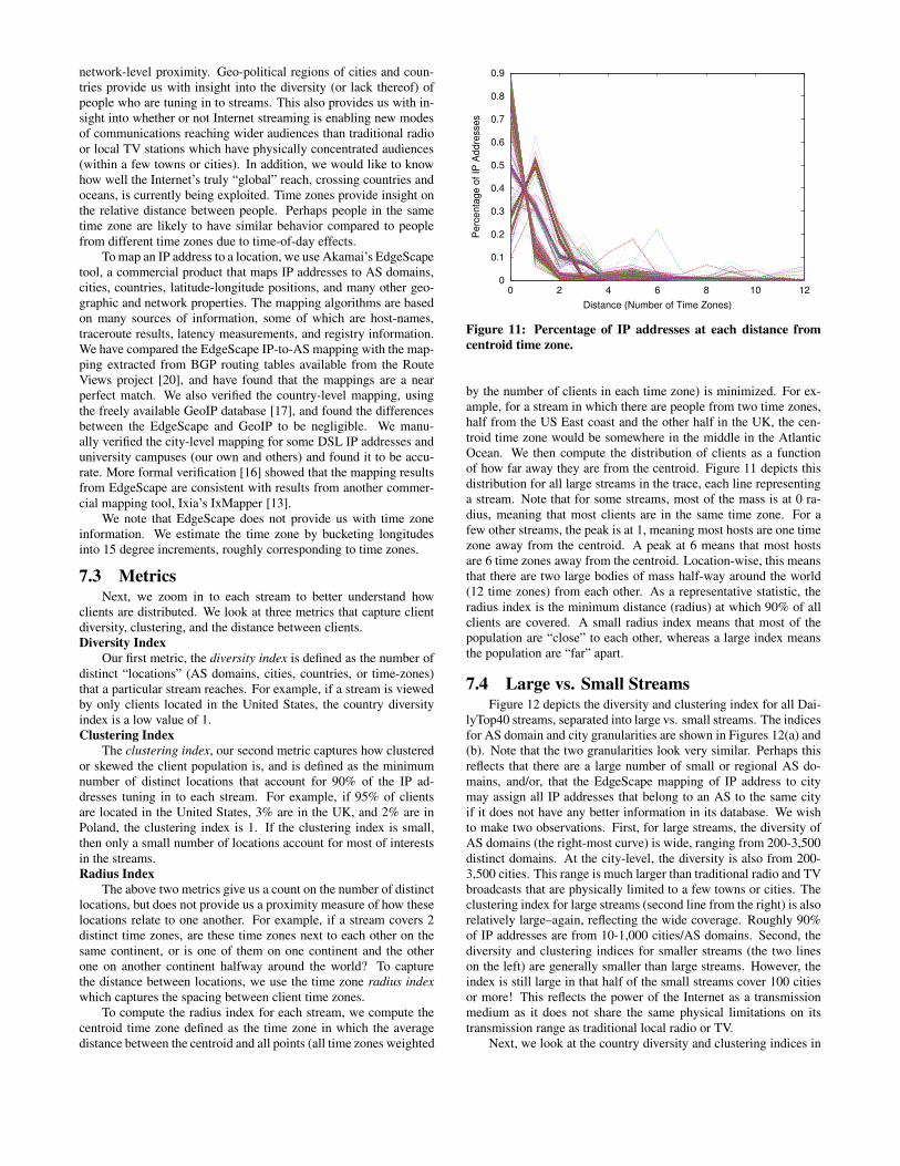
Figure 11: Percentage of IP addresses at each distance fromcentroid time zone.
by the number of clients in each time zone) is minimized. For ex-ample, for a stream in which there are people from two time zones,half from the US East coast and the other half in the UK, the cen-troid time zone would be somewhere in the middle in the AtlanticOcean. We then compute the distribution of clients as a functionof how far away they are from the centroid. Figure 11 depicts thisdistribution for all large streams in the trace, each line representinga stream. Note that for some streams, most of the mass is at 0 ra-dius, meaning that most clients are in the same time zone. For afew other streams, the peak is at 1, meaning most hosts are one timezone away from the centroid. A peak at 6 means that most hostsare 6 time zones away from the centroid. Location-wise, this meansthat there are two large bodies of mass half-way around the world(12 time zones) from each other. As a representative statistic, theradius index is the minimum distance (radius) at which 90% of allclients are covered. A small radius index means that most of thepopulation are “close” to each other, whereas a large index meansthe population are “far” apart.
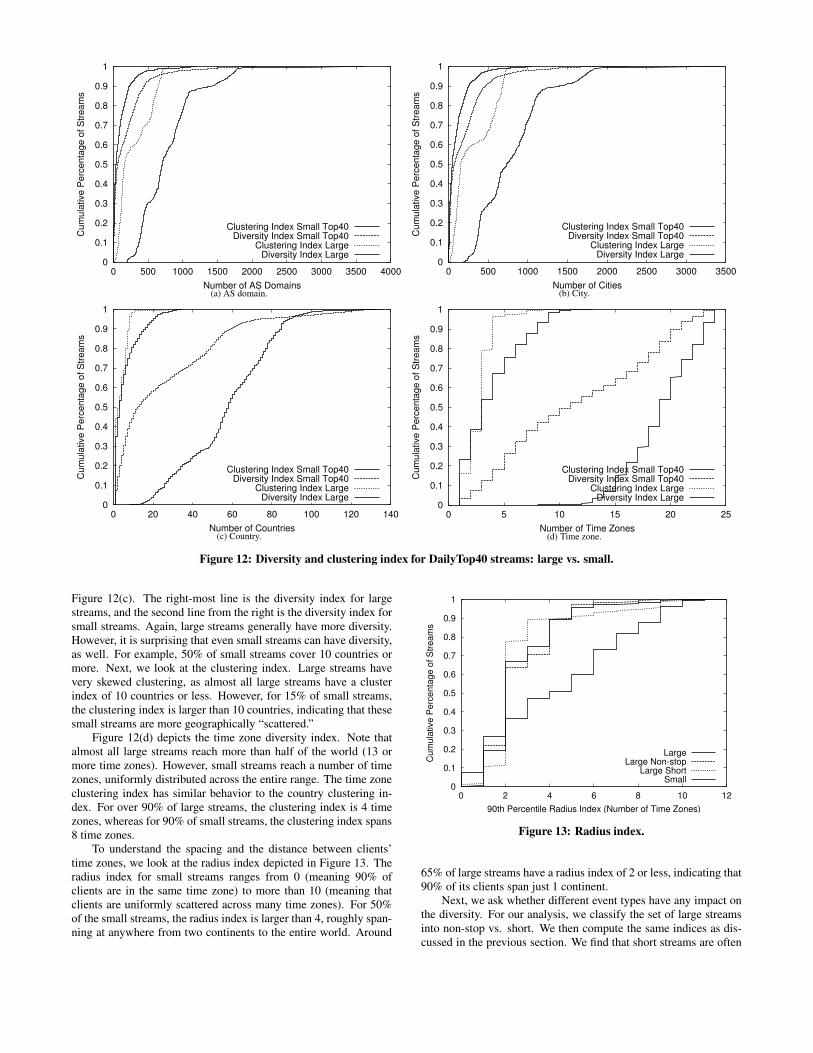
7.4 Large vs. Small StreamsFigure 12 depicts the diversity and clustering index for all Dai-
lyTop40 streams, separated into large vs. small streams. The indicesfor AS domain and city granularities are shown in Figures 12(a) and(b). Note that the two granularities look very similar. Perhaps thisreflects that there are a large number of small or regional AS do-mains, and/or, that the EdgeScape mapping of IP address to citymay assign all IP addresses that belong to an AS to the same cityif it does not have any better information in its database. We wishto make two observations. First, for large streams, the diversity ofAS domains (the right-most curve) is wide, ranging from 200-3,500distinct domains. At the city-level, the diversity is also from 200-3,500 cities. This range is much larger than traditional radio and TVbroadcasts that are physically limited to a few towns or cities. Theclustering index for large streams (second line from the right) is alsorelatively large–again, reflecting the wide coverage. Roughly 90%of IP addresses are from 10-1,000 cities/AS domains. Second, thediversity and clustering indices for smaller streams (the two lineson the left) are generally smaller than large streams. However, theindex is still large in that half of the small streams cover 100 citiesor more! This reflects the power of the Internet as a transmissionmedium as it does not share the same physical limitations on itstransmission range as traditional local radio or TV.
Next, we look at the country diversity and clustering indices in
0
0.1
0.2
0.3
0.4
0.5
0.6
0.7
0.8
0.9
1
0 500 1000 1500 2000 2500 3000 3500 4000
Cum
ulat
ive
Per
cent
age
of S
tream
s
Number of AS Domains
Clustering Index Small Top40Diversity Index Small Top40
Clustering Index LargeDiversity Index Large
(a) AS domain.
0
0.1
0.2
0.3
0.4
0.5
0.6
0.7
0.8
0.9
1
0 500 1000 1500 2000 2500 3000 3500
Cum
ulat
ive
Per
cent
age
of S
tream
s
Number of Cities
Clustering Index Small Top40Diversity Index Small Top40
Clustering Index LargeDiversity Index Large
(b) City.
0
0.1
0.2
0.3
0.4
0.5
0.6
0.7
0.8
0.9
1
0 20 40 60 80 100 120 140
Cum
ulat
ive
Per
cent
age
of S
tream
s
Number of Countries
Clustering Index Small Top40Diversity Index Small Top40
Clustering Index LargeDiversity Index Large
(c) Country.
0
0.1
0.2
0.3
0.4
0.5
0.6
0.7
0.8
0.9
1
0 5 10 15 20 25
Cum
ulat
ive
Per
cent
age
of S
tream
s
Number of Time Zones
Clustering Index Small Top40Diversity Index Small Top40
Clustering Index LargeDiversity Index Large
(d) Time zone.
Figure 12: Diversity and clustering index for DailyTop40 streams: large vs. small.
Figure 12(c). The right-most line is the diversity index for largestreams, and the second line from the right is the diversity index forsmall streams. Again, large streams generally have more diversity.However, it is surprising that even small streams can have diversity,as well. For example, 50% of small streams cover 10 countries ormore. Next, we look at the clustering index. Large streams havevery skewed clustering, as almost all large streams have a clusterindex of 10 countries or less. However, for 15% of small streams,the clustering index is larger than 10 countries, indicating that thesesmall streams are more geographically “scattered.”
Figure 12(d) depicts the time zone diversity index. Note thatalmost all large streams reach more than half of the world (13 ormore time zones). However, small streams reach a number of timezones, uniformly distributed across the entire range. The time zoneclustering index has similar behavior to the country clustering in-dex. For over 90% of large streams, the clustering index is 4 timezones, whereas for 90% of small streams, the clustering index spans8 time zones.
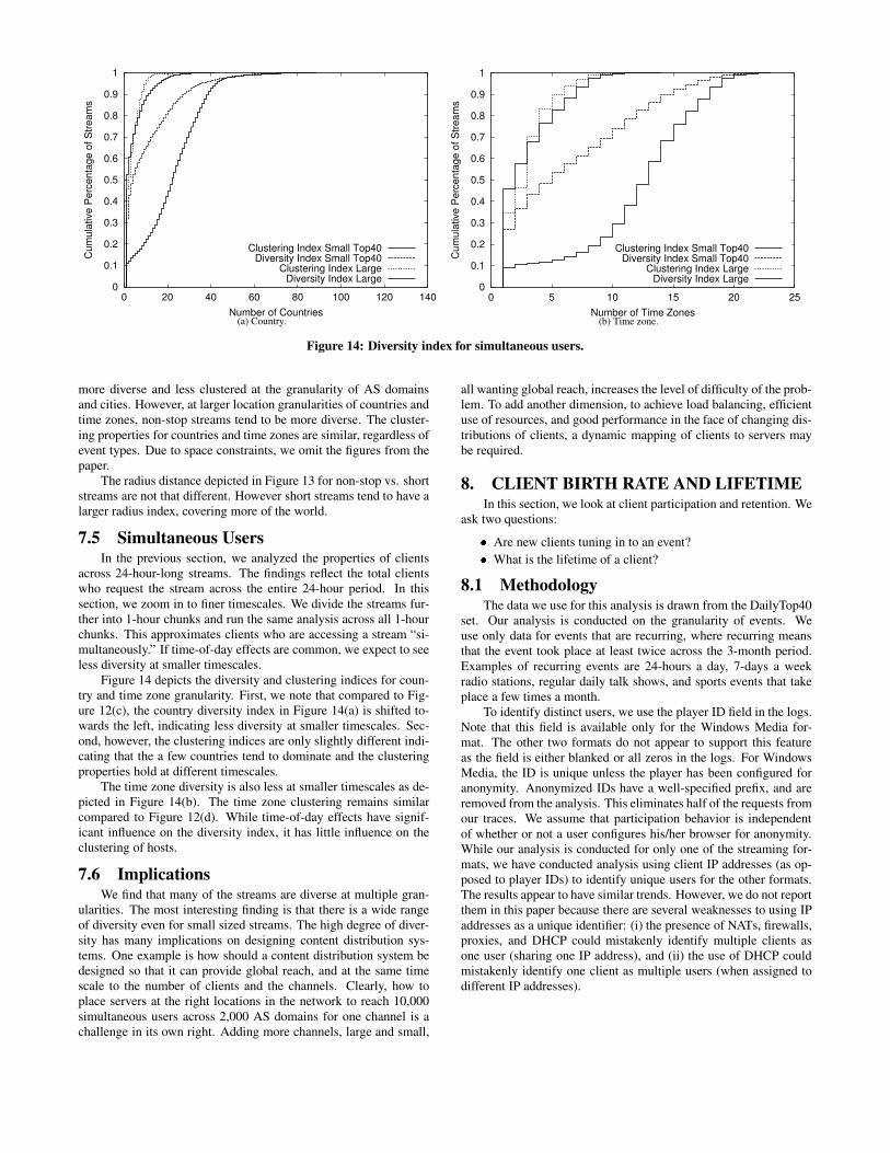
To understand the spacing and the distance between clients’time zones, we look at the radius index depicted in Figure 13. Theradius index for small streams ranges from 0 (meaning 90% ofclients are in the same time zone) to more than 10 (meaning thatclients are uniformly scattered across many time zones). For 50%of the small streams, the radius index is larger than 4, roughly span-ning at anywhere from two continents to the entire world. Around
0
0.1
0.2
0.3
0.4
0.5
0.6
0.7
0.8
0.9
1
0 2 4 6 8 10 12
Cum
ulat
ive
Per
cent
age
of S
tream
s
90th Percentile Radius Index (Number of Time Zones)
LargeLarge Non-stop
Large ShortSmall
Figure 13: Radius index.
65% of large streams have a radius index of 2 or less, indicating that90% of its clients span just 1 continent.
Next, we ask whether different event types have any impact onthe diversity. For our analysis, we classify the set of large streamsinto non-stop vs. short. We then compute the same indices as dis-cussed in the previous section. We find that short streams are often
0
0.1
0.2
0.3
0.4
0.5
0.6
0.7
0.8
0.9
1
0 20 40 60 80 100 120 140
Cum
ulat
ive
Per
cent
age
of S
tream
s
Number of Countries
Clustering Index Small Top40Diversity Index Small Top40
Clustering Index LargeDiversity Index Large
(a) Country.
0
0.1
0.2
0.3
0.4
0.5
0.6
0.7
0.8
0.9
1
0 5 10 15 20 25
Cum
ulat
ive
Per
cent
age
of S
tream
s
Number of Time Zones
Clustering Index Small Top40Diversity Index Small Top40
Clustering Index LargeDiversity Index Large
(b) Time zone.
Figure 14: Diversity index for simultaneous users.
more diverse and less clustered at the granularity of AS domainsand cities. However, at larger location granularities of countries andtime zones, non-stop streams tend to be more diverse. The cluster-ing properties for countries and time zones are similar, regardless ofevent types. Due to space constraints, we omit the figures from thepaper.
The radius distance depicted in Figure 13 for non-stop vs. shortstreams are not that different. However short streams tend to have alarger radius index, covering more of the world.
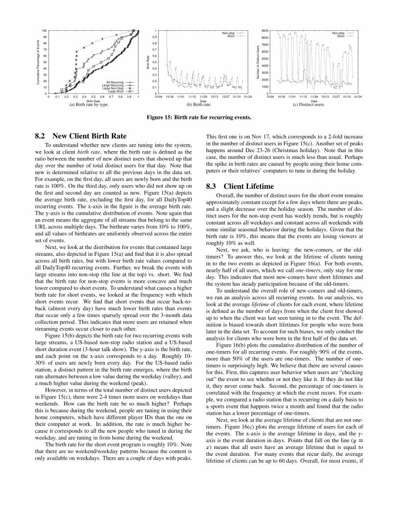
7.5 Simultaneous UsersIn the previous section, we analyzed the properties of clients
across 24-hour-long streams. The findings reflect the total clientswho request the stream across the entire 24-hour period. In thissection, we zoom in to finer timescales. We divide the streams fur-ther into 1-hour chunks and run the same analysis across all 1-hourchunks. This approximates clients who are accessing a stream “si-multaneously.” If time-of-day effects are common, we expect to seeless diversity at smaller timescales.
Figure 14 depicts the diversity and clustering indices for coun-try and time zone granularity. First, we note that compared to Fig-ure 12(c), the country diversity index in Figure 14(a) is shifted to-wards the left, indicating less diversity at smaller timescales. Sec-ond, however, the clustering indices are only slightly different indi-cating that the a few countries tend to dominate and the clusteringproperties hold at different timescales.
The time zone diversity is also less at smaller timescales as de-picted in Figure 14(b). The time zone clustering remains similarcompared to Figure 12(d). While time-of-day effects have signif-icant influence on the diversity index, it has little influence on theclustering of hosts.
7.6 ImplicationsWe find that many of the streams are diverse at multiple gran-
ularities. The most interesting finding is that there is a wide rangeof diversity even for small sized streams. The high degree of diver-sity has many implications on designing content distribution sys-tems. One example is how should a content distribution system bedesigned so that it can provide global reach, and at the same timescale to the number of clients and the channels. Clearly, how toplace servers at the right locations in the network to reach 10,000simultaneous users across 2,000 AS domains for one channel is achallenge in its own right. Adding more channels, large and small,
all wanting global reach, increases the level of difficulty of the prob-lem. To add another dimension, to achieve load balancing, efficientuse of resources, and good performance in the face of changing dis-tributions of clients, a dynamic mapping of clients to servers maybe required.
8. CLIENT BIRTH RATE AND LIFETIMEIn this section, we look at client participation and retention. We
ask two questions:� Are new clients tuning in to an event?� What is the lifetime of a client?
8.1 MethodologyThe data we use for this analysis is drawn from the DailyTop40
set. Our analysis is conducted on the granularity of events. Weuse only data for events that are recurring, where recurring meansthat the event took place at least twice across the 3-month period.Examples of recurring events are 24-hours a day, 7-days a weekradio stations, regular daily talk shows, and sports events that takeplace a few times a month.
To identify distinct users, we use the player ID field in the logs.Note that this field is available only for the Windows Media for-mat. The other two formats do not appear to support this featureas the field is either blanked or all zeros in the logs. For WindowsMedia, the ID is unique unless the player has been configured foranonymity. Anonymized IDs have a well-specified prefix, and areremoved from the analysis. This eliminates half of the requests fromour traces. We assume that participation behavior is independentof whether or not a user configures his/her browser for anonymity.While our analysis is conducted for only one of the streaming for-mats, we have conducted analysis using client IP addresses (as op-posed to player IDs) to identify unique users for the other formats.The results appear to have similar trends. However, we do not reportthem in this paper because there are several weaknesses to using IPaddresses as a unique identifier: (i) the presence of NATs, firewalls,proxies, and DHCP could mistakenly identify multiple clients asone user (sharing one IP address), and (ii) the use of DHCP couldmistakenly identify one client as multiple users (when assigned todifferent IP addresses).
0
10
20
30
40
50
60
70
80
90
100
0 0.1 0.2 0.3 0.4 0.5 0.6 0.7 0.8 0.9 1
Cum
ulat
ive
Per
cent
age
of E
vent
s
Birth Rate
All RecurringLarge RecurringLarge Non-Stop
Large Short
(a) Birth rate by type.
0
0.1
0.2
0.3
0.4
0.5
0.6
0.7
0.8
0.9
1
10/04 10/18 11/01 11/15 11/29 12/13 12/27 01/10 01/24
Birt
h R
ate
Date
Non-stopShort
(b) Birth rate.
0
1000
2000
3000
4000
5000
6000
7000
8000
9000
10/04 10/18 11/01 11/15 11/29 12/13 12/27 01/10 01/24
Num
ber o
f Dis
tinct
Use
rs
Date
Non-stopShort
(c) Distinct users.
Figure 15: Birth rate for recurring events.
8.2 New Client Birth RateTo understand whether new clients are tuning into the system,
we look at client birth rate, where the birth rate is defined as theratio between the number of new distinct users that showed up thatday over the number of total distinct users for that day. Note thatnew is determined relative to all the previous days in the data set.For example, on the first day, all users are newly born and the birthrate is 100%. On the third day, only users who did not show up onthe first and second day are counted as new. Figure 15(a) depictsthe average birth rate, excluding the first day, for all DailyTop40recurring events. The x-axis in the figure is the average birth rate.The y-axis is the cumulative distribution of events. Note again thatan event means the aggregate of all streams that belong to the sameURL across multiple days. The birthrate varies from 10% to 100%,and all values of birthrates are uniformly observed across the entireset of events.
Next, we look at the distribution for events that contained largestreams, also depicted in Figure 15(a) and find that it is also spreadacross all birth rates, but with lower birth rate values compared toall DailyTop40 recurring events. Further, we break the events withlarge streams into non-stop (the line at the top) vs. short. We findthat the birth rate for non-stop events is more concave and muchlower compared to short events. To understand what causes a higherbirth rate for short events, we looked at the frequency with whichshort events recur. We find that short events that occur back-to-back (almost every day) have much lower birth rates than eventsthat occur only a few times sparsely spread over the 3-month datacollection period. This indicates that more users are retained whenstreaming events occur closer to each other.
Figure 15(b) depicts the birth rate for two recurring events withlarge streams, a US-based non-stop radio station and a US-basedshort duration event (3-hour talk show). The y-axis is the birth rate,and each point on the x-axis corresponds to a day. Roughly 10-30% of users are newly born every day. For the US-based radiostation, a distinct pattern in the birth rate emerges, where the birthrate alternates between a low value during the weekday (valley), anda much higher value during the weekend (peak).
However, in terms of the total number of distinct users depictedin Figure 15(c), there were 2-4 times more users on weekdays thanweekends. How can the birth rate be so much higher? Perhapsthis is because during the weekend, people are tuning in using theirhome computers, which have different player IDs than the one ontheir computer at work. In addition, the rate is much higher be-cause it corresponds to all the new people who tuned in during theweekday, and are tuning in from home during the weekend.
The birth rate for the short event program is roughly 10%. Notethat there are no weekend/weekday patterns because the content isonly available on weekdays. There are a couple of days with peaks.
This first one is on Nov 17, which corresponds to a 2-fold increasein the number of distinct users in Figure 15(c). Another set of peakshappens around Dec 23-26 (Christmas holiday). Note that in thiscase, the number of distinct users is much less than usual. Perhapsthe spike in birth rates are caused by people using their home com-puters or their relatives’ computers to tune in during the holiday.
8.3 Client LifetimeOverall, the number of distinct users for the short event remains
approximately constant except for a few days where there are peaks,and a slight decrease over the holiday season. The number of dis-tinct users for the non-stop event has weekly trends, but is roughlyconstant across all weekdays and constant across all weekends withsome similar seasonal behavior during the holidays. Given that thebirth rate is 10%, this means that the events are losing viewers atroughly 10% as well.
Next, we ask, who is leaving: the new-comers, or the old-timers? To answer this, we look at the lifetime of clients tuningin to the two events as depicted in Figure 16(a). For both events,nearly half of all users, which we call one-timers, only stay for oneday. This indicates that most new-comers have short lifetimes andthe system has steady participation because of the old-timers.
To understand the overall role of new-comers and old-timers,we run an analysis across all recurring events. In our analysis, welook at the average lifetime of clients for each event, where lifetimeis defined as the number of days from when the client first showedup to when the client was last seen tuning in to the event. The def-inition is biased towards short lifetimes for people who were bornlater in the data set. To account for such biases, we only conduct theanalysis for clients who were born in the first half of the data set.
Figure 16(b) plots the cumulative distribution of the number ofone-timers for all recurring events. For roughly 90% of the events,more than 50% of the users are one-timers. The number of one-timers is surprisingly high. We believe that there are several causesfor this. First, this captures user behavior when users are “checkingout” the event to see whether or not they like it. If they do not likeit, they never come back. Second, the percentage of one-timers iscorrelated with the frequency at which the event recurs. For exam-ple, we compared a radio station that is recurring on a daily basis toa sports event that happens twice a month and found that the radiostation has a lower percentage of one-timers.
Next, we look at the average lifetime of clients that are not one-timers. Figure 16(c) plots the average lifetime of users for each ofthe events. The x-axis is the average lifetime in days, and the y-axis is the event duration in days. Points that fall on the line ( ���� ) means that all users have an average lifetime that is equal tothe event duration. For many events that recur daily, the averagelifetime of clients can be up to 60 days. Overall, for most events, if

0
0.1
0.2
0.3
0.4
0.5
0.6
0.7
0.8
0.9
1
0 10 20 30 40 50 60 70 80 90 100
Cum
ulat
ive
Per
cent
age
of U
sers
Life Time (Days)
Non-stopShort
(a) Lifetime for two recurring events.
0
0.1
0.2
0.3
0.4
0.5
0.6
0.7
0.8
0.9
1
0.1 0.2 0.3 0.4 0.5 0.6 0.7 0.8 0.9 1
Cum
ulat
ive
Per
cent
age
of E
vent
s
Percentage of One-Timers(b) Percentage of one-timers in each event.
0
10
20
30
40
50
60
70
80
90
100
0 10 20 30 40 50 60 70
Eve
nt D
urat
ion
(Day
s)
Life Time (Days)(c) Average client lifetime excluding one-timers.
Figure 16: Client lifetime.
a client shows up more than once, it will have an average lifetimeof at least one-third of the days in the event.
8.4 ImplicationsTo summarize, we have shown that for all events the birth rate
for new clients tuning in is roughly 10% or more. Roughly 50% ormore new clients are one-timers. However, the events have steadymembership because there are enough old-timers that have high av-erage lifetimes. To understand the significance of our findings, wepresent two examples of design decisions where our observationscan be applied. First, the presence of one-timers has direct implica-tions on the scalability of maintaining per-client “persistent” state atservers. Such state may be used by the server to customize contentserved to clients. To control the amount of overhead in maintainingstate, a caching-based algorithm can be used to rapidly time-out onthe one-timers, which are at least 50% of the client base. A sec-ond example is that clients can maintain performance history forthe servers that it visits. Given that clients keep accessing the sameevent/server repeatedly over many days, history should be useful forserver selection problems.
9. RELATED WORKLive streaming and MBone workloads
Veloso et al. [23] studied live streaming workloads from a serverlocated in Brazil. The focus of the analysis was on characterizing ar-rival processes and session durations for two non-stop video eventsto be used in a workload generator. Our findings for arrival pro-cesses and session durations from the Akamai workloads are con-sistent with their findings. However, to contrast, we have also an-alyzed several other properties such as the popularity of streams,the use of transport protocols, the diversity of clients, and the clientlifetime.
The join arrival process and session duration distribution formulticast groups on the MBone were also analyzed [3]. The keyfindings were that interarrivals follow an exponential distribution,and durations fit a Zipf distribution for non-stop multicast groups.For a group with short duration (for example, a 1-hour lecture),the session durations are exponential. While the interarrival find-ings are similar to our workload, the session durations are different.We identified that session durations are heavy-tailed irrespective ofwhether or not the stream is non-stop vs short duration. However,the shape of the tail is different (Pareto vs. truncated) for differentstream types.Location of users
Faloutsos et al. [8] looked at “spatial clustering” amongst usersin (i) Quake I, a network game, and (ii) MBone multicast groups.They focused on AS-level clustering inside a group and correlationsamongst groups. They found that for network games, there is lit-
tle clustering. However, there is significant clustering for multicastgroups. While we also look at AS-level clustering, we also look atgeographical and time-zone clustering. In addition, the number of“members” of streams in our data set is orders of magnitudes larger.
AS clustering amongst clients accessing the same web-site hasalso been studied [14]. The key findings are that cluster sizes areheavily skewed. There are a few very large clusters, and a numberof small clusters. In contrast to this study, we are also interested inhow these clusters relate to each other in terms of their distance. Welook at whether these clusters span the globe, or are concentrated inone geographical location.Web, on-demand streaming, and peer-to-peer workloads
Many studies of Web workloads have found that the popular-ity of Web objects follows a Zipf distribution [11, 9, 15, 2, 5].In contrast, we have found that the popularity distribution for livestreaming has two modes where the first mode (head) is flatter thanthe second mode (tail). Studies of on-demand streaming work-loads have also observed a popularity distribution with one [6] ortwo modes [1]. Session durations often exhibited heavy-tail behav-ior, similar to what we have observed for live streaming. In addi-tion, session interarrivals were found to be approximately exponen-tial during periods of stationary request arrivals. More recently, abimodal popularity distribution was also observed in peer-to-peermultimedia file-sharing workloads [12].
The join arrival process, session duration distribution, user di-versity, and new host birth rate was analyzed for End System Multi-cast (ESM), a peer-to-peer live streaming system with streams thatattract 100-1,000’s of users [21]. Overall the ESM and Akamai livestreaming workloads are similar. The join interarrival distributionis exponential and the session duration distribution is log-normal.Similar tail behavior for short duration events were also observed.Despite the small scale deployment, there is a wide diversity in userpopulation with users from more than 15 countries participatingin any one stream. Finally, new host birth rate for back-to-backstreams was roughly 50% which is high, but slightly lower than theaverage birth rate of 64% for Akamai streams.
10. SUMMARYIn this paper, we analyzed 3-months of live streaming work-
loads from a large content distribution network. We take a macro-scopic approach to identify common trends amongst the varioustypes of content. Specifically, from our data set, we found that:
� Most of the live streaming workload today is audio. Only 1%of the requests are for video streams. And only 7% of streamsare video streams.� A small number of events, mostly non-stop audio programslike radio, account for a huge fraction of the requests. Thepopularity distribution is Zipf-like with two distinct modes.
� Non-stop streams have strong time-of-day and time zone cor-related behavior. In addition, a surprisingly large number ofstreams exhibit flash crowd behavior. We find that 50% of alllarge streams, non-stop and short duration, have flash crowds.� Almost half of the AS domains seen in our logs tend to useTCP as the dominant transport protocol. Such characteristicscould perhaps be caused by the presence of network addresstranslators (NATs) and firewalls that disallow the use of UDP.� The diversity of clients accessing live streams on the Internetis much wider than traditional broadcast media such as radioand local TV. Almost all large streams reach 13 or more dif-ferent time zones, 10 or more different countries, and 200 ormore different AS domains. Half of the small streams reach11 or more different time zones, 10 or more different coun-tries, and 100 or more different AS domains.� Client lifetime is bimodal. Half of the new clients who tunein to a stream will tune in for only one day. For the remaininghalf, their average lifetime is at least as long as one-third ofthe days in the event.
Our work is a first step in understanding live streaming work-loads on the Internet. There are several directions that we wish topursue as future work. One important aspect is to study the implica-tions of the workloads on the system design. A second direction is tounderstand how the workloads may change over time and under dif-ferent operating environments. For example, in a few years, the last-mile bottleneck to the home may change from cable modem/DSL tofiber. In such conditions, will there be more high-bandwidth videocontent? Will bandwidth growth spur the development of new ap-plications that could dramatically change the use of live streamingon the Internet? If anyone on the Internet, as opposed to profes-sional publishers, can publish high-bandwidth content, would therebe orders of magnitude more small-scale groups with more diversityin the client population?
AcknowledgementsWe wish to thank Roberto De Prisco of the University of Salernoand Akamai Technologies, for assistance with collecting log datafrom the Akamai streaming servers. We also thank the anonymousreviewers for their valuable feedback.
11. REFERENCES[1] J. M. Almeida, J. Krueger, D. L. Eager, and M. K. Vernon.
Analysis of Educational Media Server Workloads. InProceedings of NOSSDAV, June 2001.
[2] V. Almeida, A. Bestavros, M. Crovella, and A. de Oliveira.Characterizing Reference Locality in the WWW. InProceedings of 1996 International Conference on Paralleland Distributed Information Systems (PDIS ’96), 1996.
[3] K. C. Almeroth and M. H. Ammar. Collecting and Modelingthe Join/Leave Behavior of Multicast Group Members in theMBone. In Proceedings of International Symposium on HighPerformance Distributed Computing (HPDC), August 1996.
[4] K. Andreev, B. M. Maggs, A. Meyerson, and R. Sitaraman.Designing Overlay Multicast Networks for Streaming. InProceedings of the Fifteenth Annual ACM Symposium onParallel Algorithms and Architectures (SPAA), 2003.
[5] L. Breslau, P. Cao, L. Fan, G. Phillips, and S. Shenker. WebCaching and Zipf-like Distributions: Evidence andImplications. In Proceedings of the IEEE INFOCOMM ’99,March 1999.
[6] M. Chesire, A. Wolman, G. Voelker, and H. Levy.Measurement and Analysis of a Streaming-Media Workload.
In Proceedings of Usenix Symposium on InternetTechnologies and Systems (USITS), March 2001.
[7] M. Crovella and M. Taqqu. Estimating the Heavy Tail Indexfrom Scaling Properties. In Methodology and Computing inApplied Probability, vol. 1, no. 1, 1999.
[8] J. Cui, M. Faloutsos, D. Maggiorini, M. Gerla, andK. Boussetta. Measuring and Modelling the GroupMembership in the Internet. In Proceedings of InternetMeasurement Conference (IMC), October 2003.
[9] C. Cunha, A. Bestavros, and M. Covella. Characteristics ofWWW Client Based Traces. Technical ReportBU-CS-95-010, Computer Science Department, BostonUniversity, 1995.
[10] S. Floyd, M. Handley, J. Padhye, and J. Widmer. MulticastRouting in Internetworks and Extended LANs. InProceedings of the ACM SIGCOMM, August 2000.
[11] S. Glassman. A Caching Relay for the World Wide Web. InProceedings of the First International Conference on theWorld-Wide Web, 1994.
[12] K. Gummadi, R. Dunn, S. Saroiu, S. Gribble, H. Levy, andJ. Zahorjan. Measurement, Modeling, and Analysis of aPeer-to-Peer File-Sharing Workload. In Proceedings of ACMSOSP, October 2003.
[13] IxMapper. http://www.ixiacom.com/products.[14] B. Krishnamurthy and J. Wang. On Network-Aware
Clustering of Web Clients. In Proceedings of ACMSIGCOMM, September 2000.
[15] T. M. Kroeger, J. C. Mogul, and C. Maltzahn. Digital’s webproxy traces. Available atftp://ftp.digital.com/pub/DEC/traces/proxy/webtraces.html,August 1996.
[16] A. Lakhina, J. W. Byers, M. Crovella, and I. Matta. On theGeographic Location of Internet Resources. In IEEE Journalon Selected Areas in Communications Vol. 21 No. 6, Aug2003.
[17] MaxMind GeoIP Free Country Database.http://www.maxmind.com/app/geoip country.
[18] Microsoft Windows Media Services 9 Series and WindowsMedia Services Version 4.1 - Performance Comparison.http://www.veritest.com/clients/reports/microsoft/ms media services.pdf.
[19] V. N. Padmanabhan, H. J. Wang, P. A. Chou, andK. Sripanidkulchai. Distributing Streaming Media ContentUsing Cooperative Networking. In Proceedings of NOSSDAV,May 2002.
[20] Route Views Project. http://www.routeviews.org/.[21] K. Sripanidkulchai. A Measurement-Driven Approach to
Designing Peer-to-Peer Systems. Ph.D. Thesis, CarnegieMellon University, 2004.
[22] K. Sripanidkulchai, A. Ganjam, B. Maggs, and H. Zhang.The Feasibility of Supporting Large-Scale Live StreamingApplications with Dynamic Application End-Points. InProceedings of ACM SIGCOMM, 2004.
[23] E. Veloso, V. Almeida, W. Meira, A. Bestavros, and S. Jin. AHierarchical Characterization of a Live Streaming MediaWorkload. In Proceedings of Internet Measurement Workshop(IMW), November 2002.
[24] Y. Wang, M. Claypool, and Z. Zuo. An Empirical Study ofRealVideo Performance Across the Internet. In Proceedingsof Internet Measurement Workshop (IMW), November 2001.