an analysis of algorithms for in vivo fiber tractography
TRANSCRIPT

An Analysis of Algorithms for In Vivo Fiber Tractography Using DW-MRI Data
780 Project
Jing Li
Supervised by: Dr. Burkhard Wuensche
The Computer Science Department
The University of Auckland
2005

ABSTRACT
In this paper, several nerve fiber tracking methods which are used to visualize the
connectivity of brain regions in vivo are analyzed using noise-affected synthetic diffusion
tensor fields with crossing tracts geometry. The simulated DTI dataset is constructed
using B-Spline curves wrapped with a tube, which represents a bundle of never fiber
tracts. Particularly, we compare three fiber tractography methods, Streamlines,
Tensorlines, and Tensor deflection (TEND). The analysis of the simulations revealed that
when estimating the crossing trajectories of white matter tracts in human brain,
Streamlines simulation completely deviate from the ideal pathway, whereas Tensorlines
and TEND methods keep a part of integrated tracts inside the ideal pathway, and are
suitable to be used to simulate the tracts of a diffusion tensor field with crossing,
branching, merging and brunching tracts geometries.

Contents
INTRODUCTION ........................................................................................................................................ 1 DIFFUSION TENSOR MAGNETIC RESONANCE IMAGING............................................................ 3
DTI DATA ACQUISITION.............................................................................................................................. 3 DTI DATA PROCESSING............................................................................................................................... 4 LIMITATION OF DIFFUSION TENSOR IMAGING ............................................................................................. 7
FIBER TRACTOGRAPHY MEHTODS ................................................................................................... 8 STREAMLINE TRACKING ............................................................................................................................. 8 TENSORLINE ALGORITHM ......................................................................................................................... 10 TENSOR DEFLECTION................................................................................................................................ 10
SYNTHETIC TENSOR FIELD................................................................................................................ 12 CONSTRUCTION OF EIGENVALUES AND EIGENVECTORS........................................................................... 12 SIMULATION PROCEDURE FOR ADDING NOISE TO A SYNTHETIC TENSOR FIELD ......................................... 13
IMPLEMENTATION................................................................................................................................ 16 CONSTRUCTION OF A SYNTHETIC TENSOR FIELD ..................................................................................... 16 GENERATING OF NOISED-CONTAMINATED SYNTHETIC TENSOR FIELDS..................................................... 18 SIMULATIONS OF FIBER TRACKS ............................................................................................................... 19 SOFTWARE ARCHITECTURE OF THE APPLICATION ..................................................................................... 21 USER GUIDE ............................................................................................................................................. 22
ERROR MEASUREMENTS..................................................................................................................... 24 ERROR MEASUREMENTS OF A SYNTHETIC TENSOR FIELD CONTAINING CROSSING TRACTS....................... 24
Error measurements of the average length of the simulated tracts..................................................... 24 Error measurements of the correctness of the simulated tracts .......................................................... 26 Least Square Error of the simulated tracts ......................................................................................... 29
ERROR MEASUREMENTS OF A SYNTHETIC TENSOR FIELD CONTAINING MERGING TRACTS........................ 31 Error measurements of the average length of the simulated tracts..................................................... 32 Error measurements of the correctness of the simulated tracts .......................................................... 34 Least Square Error of the simulated tracts ......................................................................................... 36
CONCLUSIONS......................................................................................................................................... 38 ACKNOWLEDGEMENTS ....................................................................................................................... 39 REFERENCES ........................................................................................................................................... 39

INTRODUCTION
Diffusion tensor image measures diffusion properties of water inside living
fibrous tissues such as nerves, muscles, ligaments, tendons, etc. (Basser, Pajevic et al.
2000). The diffusion tensor defines the directions of highest and lowest diffusion and
the diffusion coefficients in these directions of water in the living tissues. The
directional information of water diffusion in the brain can estimate the structure and
the orientation of the never fiber tracts as water tends to diffuse within white matter
along the axonal fiber direction in brain (Figure 1).
Figure 1: The basic structure of a nerve cell [1].
Nerve fiber tractography using DTI is a promising medical research tool for
studying and visualizing the nerve fiber tracts in vivo. Streamline algorithm can be
used to propagate the nerve fiber trajectories from a vector field which is computed
from the diffusion tensor field. It uses only the tensor major diffusion direction to
estimate the fiber direction, hence it fails to accurately follow the ideal pathways
when it meets the degenerated points as on such points the there are no particular
diffusion directions. To remedy such fault, the Tensorlines algorithm (Weinstein,
Kindlmann et al. 1999) incorporates information about the nearby orientation of the
local tensor to propagate stable tracts, and the Tensor Deflection algorithm (TEND)
1

(Lazar, Weinstein et al. 2003) uses the entire diffusion tensor information to deflect
the estimated fiber trajectory.
The three tractography methods, Streamlines, Tensorlines, and Tensor Deflection
were implemented in the project. To compare and analyze the three tractography
methods, synthetic diffusion tensor fields with crossing tracts are constructed. The
tracts simulated by the methods are compared with the ideal pathways of the synthetic
tensor fields that are well known in advance. To make the dataset more realistic,
Complex Gaussian normal noises with different levels of SNR are added to the real
and imaginary channels of the ideal signal for every voxel in the tensor fields (Skare,
Li et al. 2000; Jonasson, Hagmann et al. 2003).
2

DIFFUSION TENSOR MAGNETIC RESONANCE IMAGING
The Diffusion tensor T is a symmetric second-order tensor and is presented by a
3x3 symmetric, semi-positive definite matrix only using 6 independent elements
( ). zzyzyyxzxyxx DDDDDD ,,,,,
⎟⎟⎟
⎠
⎞
⎜⎜⎜
⎝
⎛
=
zzyzxz
yzyyxy
xzxyxx
DDDDDDDDD
T Equation 1
The six independent elements are determined from a set of diffusion weighted
signals. After acquisition ofT , the three principal diffusivities (eigenvalues) known as
321 ,, λλλ and diffusion directions (eigenvectors) known as can be calculated
from the tensorT as the eigenvectors and the eigenvalues fulfill the equator Eq. [2]
(Young 1993).
321 ,, eee
⎟⎟⎟
⎠
⎞
⎜⎜⎜
⎝
⎛
⎟⎟⎟
⎠
⎞
⎜⎜⎜
⎝
⎛=
⎟⎟⎟
⎠
⎞
⎜⎜⎜
⎝
⎛
3
2
1
3
2
1
3
2
1
000000
eee
eee
Tλ
λλ
Equation 2
DTI data acquisition
A diffusion tensor image is estimated from a series of diffusion weighted images
that are acquired with applied different diffusion weighted gradient direction vectors.
Two commonly used DTI schemes employ 6 or 7 diffusion weighted gradient
directions. The relationship of the diffusion weighted (DW) pixel intensity , the
tensor T and DW gradient vector is described by the equation Eq. [3] (Papadakis,
Xing et al. 1999).
S
)exp(0 dTd GTBGSS ••−= Equation 3
where is the baseline pixel intensity with the DW gradients are set to zero; is
the unit vector describing the DW gradient direction;
0S dG
B is called the b-factor, which
does not rely on DW gradient direction at all. and0S B are usually constants for a
tensor field.
We look at the details of the matrix production of . dTd GTG ••
3
( )
( )
( )
⎟⎟⎟⎟⎟⎟⎟⎟
⎠
⎞
⎜⎜⎜⎜⎜⎜⎜⎜
⎝
⎛
•=
+++++=
⎟⎟⎟
⎠
⎞
⎜⎜⎜
⎝
⎛•++++++=
⎟⎟⎟
⎠
⎞
⎜⎜⎜
⎝
⎛•⎟⎟⎟
⎠
⎞
⎜⎜⎜
⎝
⎛
•=••
yz
xz
xy
zz
yy
xx
dzdydzdxdxdxdzdydx
yzdzdyxzdzdxxydxdxzzdzyydyxxdx
dz
dy
dx
zzdzyzdyxzdxyzdzyydyxydxxzdzxydyxxdx
dz
dy
dx
zzyzxz
yzyyxy
xzxyxx
dzdydxdTd
DDDDDD
GGGGGGGGG
DGGDGGDGGDGDGDG
GGG
DGDGDGDGDGDGDGDGDG
GGG
DDDDDDDDD
GGGGTG
222
222
222
222
Defining the six-dimensional (6D) vectors
( )dzdydzdxdxdxdzdydx GGGGGGGGGg 222222= ,
( )Tyzxzxyzzyyxx DDDDDDt = , as a result, the Eq.[3] can be rewritten to )exp(0 tBgSS •−= , then we have
)ln(1 0
SS
Btg =• Equation 4
Provided the baseline signal , b-factor0S B , the diffusion weighted image pixel
intensity and the DW gradient direction vectors, then Eq.[4] is a linear function. By
solving it, the six unknown elements of the tensor are determined. Actually, the
S
tg • in the Eq. [4] is called the apparent diffusion coefficients (ADC) (Skare, Li et al.
2000).
DTI data processing
A general tensor is uniquely defined in terms of its three principal diffusivities
(eigenvalues: 321 ,, λλλ ) and three corresponding diffusion directions (eigenvectors:
) (Young 1993; Jonasson, Bresson et al. 2005). For a diffusion tensor field, 321 ,, eee
4

the tensor at any point is a 3x3 symmetric, semi-positive definite matrix. Its three
eigenvalues are all real and the three eigenvectors are mutually orthogonal (Young
1993). The Eq. [5] is used to construct a diffusion tensor field using three real
eigenvalues and three orthogonal eigenvectors.
( )⎟⎟⎟
⎠
⎞
⎜⎜⎜
⎝
⎛
⎟⎟⎟
⎠
⎞
⎜⎜⎜
⎝
⎛=
3
2
1
3
2
1
321
000000
eee
eeeTλ
λλ
Equation 5
where 321 λλλ ≥≥ , is the major eigenvector associated to the max eigenvalue
(
1e
1λ ), is the medium eigenvector associated to the middle eigenvalue (2e 2λ ), and
is the minor eigenvector associated to the minimum eigenvalue (
3e
3λ ).
The 1λ and determine the magnitude and direction of the primary principle axis
of the ellipsoid of the tensor. The shapes of the tensor field’s ellipsoids are described
by the
1e
321 :: λλλ ratio. Figure 2 shows the ellipsoids of a tensor field have three types
of shapes: highly prolate (e.g., 321 ,λλλ >> ) depicted in Figure 2a, oblate
(e.g., 321 λλλ >>≈ ) depicted in Figure 2b, and isotropic (e.g., 321 λλλ ≈≈ ) depicted
in Figure 2c.
(a) (b) (c)
Figure 2. Tensor shape classification: Linear case (prolate) (a), Planar case (oblate) (b) and
Spherical case (isotropic) (c).
Westin (Westin, Peled et al. 1997) introduced three definitions of linear ( ),
planar ( ) and spherical ( ) anisotropy coefficients in 1997:
lc
pc sc
321
21
λλλλλ++
−=lC Equation 6
321
32 )(2λλλ
λλ++
−=pC Equation 7
5

321
33λλλ
λ++
=sC Equation 8
The three coefficients defined by Eq. [6-8] quantify the continuum of
classifications within the three cases (linear, planar, and spherical) for real diffusion
tensor data.
If a tensor has a planar shape ellipsoid (planar anisotropy) depicted in Figure 2b or
a spherical shape ellipsoid (isotropy) depicted in Fig. 2c at a point P, the point P is a
degenerate point (Hesselink, Levy et al. 1997), at which the fiber tracts may cross,
merge, branch. The two eigenvectors with nearly equivalent eigenvalues have not
particular orientations, and span a particular plane in the case of planar anisotropy,
and water diffuses uniformly in the plane. For isotropy region, none of three
eigenvectors are individual meaningful, they have not particular orientations and span
a sphere, and water is distributed uniformly in any direction. The noise in the MRI
data may make a point as degenerate point which should not be.
The diffusion tensor has two important measurements: mean diffusivity and
anisotropy. The mean diffusivity is defined as the average of the three eigenvalues of
the tensor as Eq. [9]. The anisotropy is defined as Eq. [10] (Wuensche and Lobb
2003).
3
321 λλλλ ++=mean Equation 9
22 /))(( meanmeananisotropy ITtrace λλλ −= Equation 10
where the I is an identity 3x3 matrix.
The mean and the anisotropy are used to identify the regions of grey matter, white
matter and cerebrospinal fluid(CSF) (Pierpaoli, Jezzard et al. 1996; Wuensche and
Lobb 2003) in human brain. White matter region has the properties of
25.0≥anisotropyλ and , while CSF region with , grey
matter region with
36 1010*5 −− << meanλ 310−≥meanλ
25.0<anisotropyλ and . 36 1010*5 −− << meanλ
6

Limitation of Diffusion tensor imaging
When studying the axonal architecture using DTI data, we should understand
there are some limitations with the data due to the conventional DTI data acquisition
and processing techniques. Mori(Mori and Zijl 2002) pointed out three main
limitations: a voxel containing more than one fiber tracts with different orientations
may not be handled properly; DTI can not provide information on cellular-level fiber
connectivity, which multiple fiber tracts from individual cells may merge into or
branch out from one voxel; Afferent pathways of axonal tracts which carry
information from the sense organs towards the CNS and efferent pathways of axonal
tracts which carry signals from the CNS towards the target organs (Shahar), can not
be verified from the direction of water diffusion. Moreover, the noises generated
during the DTI acquisition processing due to several reasons such as the air, patient’s
motion, can affect the accuracy of the measured DT data, and may destroy the
property that it is semi-positive definite.
7

FIBER TRACTOGRAPHY MEHTODS
There are mainly two classification of the nerve fiber tracking methods, physics-
based and statistical methods. Streamlines, Tensorlines and Tensor deflection which
are based on the diffusion direction information of the tensor field when propagating
the tracts belong to neither category. They are simply based on the diffusion
information at a point and they are no real underlying physical or statistical methods.
To simulate the nerve fiber tracks using the three methods, first find the initial
locations (seed points) in the region of interests which are determined by the mean
diffusivity and the diffusion anisotropy, then from the starting point, bidirectional
tracks determined by the diffusion tensor T at the current position are been
propagated as the eigenvector calculated from the local tensor is without sign. The
integration is along with a certain direction which is calculated differently for
Streamline, tensor Line, and tensor deflection methods. For example, the propagating
of streamline method just follows the principal diffusion direction ( ). The tracks
were terminated where they reach the volume boundary of the tensor field or they
enter into the regions of non-interest, such as the regions of grey matter and CND in
human brain.
1e
Streamline tracking
Streamlines tracking is used on vector fields. It visualizes the structure of the
vector field. When it is employed to diffusion tensor fields, it integrates the fiber
tracts only based on the major diffusion direction ( ) of the local tensor. It is defined
as the solution to the differential equation
1e
))(()( tSvdt
tS= Equation 11
where the is the unit tangent vector at , t is the time step. The fiber
trajectories of the vector field can be generated by integrating Eq. [11] with an initial
condition which specifies a starting point of the fiber tract trajectory. The
Taylor series expansion can be used to derive a solution method. There are three most
common solvers, Euler, second-order Mid-point and fourth-order Runge-Kutta (RK4)
which take one, two and four terms of the expansion of the Taylor series respectively.
))(( tSv )(tS
0)0( SS =
8

9
The higher order the solver is, the bigger time step it can use, but more derivation
computation on each step it costs. Hence, RK4 is computational more expensive than
Mid-point (Basser, Pajevic et al. 2000; Wuensche 2004). The streamline integration
using a first order Euler method is depicted in Figure 3.
)( 1tv
)( 0tS) ( 1tS )(tS
Figure 3: Streamline integration using a first order Euler method.
The degenerate points of the tensor fields described in section “DTI processing”
need to be checked when simulating the fiber tract trajectories due to lack of
particular meaningful diffusion direction on such points and the diffusion direction
spins on a plane or a sphere (Hesselink, Levy et al. 1997). The streamline integration
should be terminated at singularity points as the fast diffusion direction is arbitrary
which will mislead the streamline propagation. Figure 4 shows such example. The
degenerate point is checked only as 21 λλ ≈ rather than at least two eigenvalues equal
(e.g. 323121 ,, λλλλλλ ≈≈≈ oror ) as the major eigenvector corresponding to the 1λ
still is meaningful on the case of 32 λλ ≈ .
Figure 4: The ideal fiber tracts path denoted by the dotted white line and the visualization of
streamline in red through anisotropy (left and right) and isotropic (middle) regions in synthetic
tensor field.

Tensorline algorithm
Weinstein(Weinstein, Kindlmann et al. 1999) introduced Tensorline fiber tracking
method in 1999. Their technique not only counts on the principal diffusion direction
of the local tensor, but also the nearby orientation information of the local tensor by
adding an advection term in a standard diffusion-based propagation method. Hence,
the propagation direction is a combination of the principal diffusion direction ( ), the
incoming vector from the previous integration step ( ) and the outgoing vector
which is the incoming vector transformed by the tensor matrix ( ).
1e
inv
outv
When doing propagation of fiber tracts, first an outgoing direction vector is
computed using the incoming direction and the tensor (Eq. [12]). The is the
direction of the previous propagation step, and the is the incoming vector
transformed by the tensor matrix.
outv
inv inv
outv
inout Tvv = Equation 12
The principal diffusion direction ( ), and are combined using Eq. [13] to
gain the proper propagation direction for current step.
1e inv outv
propv
))1)((1(1 outpunctinpunctllprop vwvwcecv +−−+= Equation 13
where, is the linear anisotropy coefficient of the local tensor computed using Eq.
[6]; is a weighting factor controlled by users, which varies from 0 to 1. The
weighting factor affects how much the propagation should be encouraged to
“puncture” to the incoming path when it goes through planar tensors by changing the
weights on the incoming vector and the outgoing vector (Weinstein, Kindlmann et al.
1999). Weinstein claimed that when integrating the fiber tracts in human brain, the
of 0.20 worked well in practice.
lc
punctw
punctw
Tensor deflection
Lazar(Lazar, Weinstein et al. 2003) introduced Tensor Deflection fiber tracking
method in 2003, which was called TEND. The method uses the entire diffusion tensor
information to deflect the incoming vector ( ) direction which is got from the
previous integration step.
inv
10

inout Tvv = Equation 14
where is the incoming vector transformed by the tensor matrix. outv
inv
1e
outv
Figure 5:Illustration of tensor deflection for a diffusion tensor
In the TEND algorithm, the incoming vector can be described using a linear
combination of the eigenvectors of the tensor.
332211 eeevin ααα ++= Equation 15
where 1α , 2α , 3α are the projections of incoming vector onto the axes of the coordinate system given by , , . 1e 2e 3e
33
22
11
evevev
in
in
in
===
ααα
Equation 16
The incoming vector is deflected toward the predominant principal eigenvector for
a tensor is more anisotropic. The less anisotropic the tensor is, the less amount the
incoming vector is deflected by the tensor.
For the formula of the Tensorlines algorithm (Eq. [13]), if equals 1, the
Tensorlines algorithm is equivalent to Streamlines method; if equals 0 and the
puncture coefficient is set to 1, the tensorlines algorithm is equivalent to Tensor
deflection method. We can see that the Tensorlines algorithm is the combination of
the Streamlines and the Tensor deflection methods.
lc
lc
punctw
11

Synthetic Tensor Field
In order to quantitatively compare the fiber tracts trajectory algorithms Synthetic
tensor fields (Westin, Maier et al. 1999; Basser, Pajevic et al. 2000; Jonasson,
Hagmann et al. 2003; Lazar and Alexander 2003; Lazar, Weinstein et al. 2003) are
required. A synthetic tensor filed is reconstructed using Eq. [5] in terms of three
eigenvalues and eigenvectors. To make the synthetic tensor more realistic, Rician
noise should be added to the tensor filed. But when the SNR of the DTI imaging is
above 3, we can approximate this noise with Gaussian normal noise.
Construction of Eigenvalues and Eigenvectors
The three eigenvalues and three eigenvectors need to be determined before
applying Eq. [5] to construct the synthetic tensor fields. Different types of fibers have
eigenvalues in certain range (Papadakis, Xing et al. 1999).
The three eigenvectors are determined by piecewise functions. In isotropic region,
they can set to uniformly distributed unit vectors which are mutually orthogonal. In
anisotropic region, the tangent unit vector of the ideal pathways of the synthetic fiber
tracts in the synthetic tensor fields is set to . Because a Frenet-frame of a space
curve is made of three vectors: tangent, normal, binormal vectors which are mutually
orthogonal, the Frenet-frame can be used to define the values for . and . Its
tangent vector indicates the direction of the pathway and is assigned to . Its normal
and binormal vectors are assigned to and respectively. The synthetic fiber tracts
should be smooth and low curvature to correspond with the natural properties of the
real never fiber tracts.
1e
1e 2e 3e
1e
2e 3e
2e 1e
3e
Figure 6: Using the Frenet-frame of a space curve to determine the eigenvectors of tensors of a synthetic tensor field.
12

Simulation procedure for adding noise to a synthetic tensor field
To make the synthetic diffusion tensor data more realistic, complex Gaussian
normal noise with zero mean and the standard deviation corresponding to the desired
SNR should be added to the real and imaginary channels of the ideal signal for every
voxel in the data. The procedure of adding noise to a synthetic tensor field is the
reverse of the process for DTI data acquisition, which solves the linear Eq. [4] to get
the six independent elements of a diffusion tensor from the baseline signal , b-
factor
0S
B , the diffusion weighted image pixel intensity and the DW gradient
direction vectors. Now, we have the noise-free tensor matrix, from that the ideal
signal can be computed. After knowing the ideal signal, we need to compute the
noised tensor with desired SNR level by assuming the baseline signal , b-factor
S
0S B ,
and the DW gradient direction vectors. The detail procedure is depicted in 7 steps
(Skare, Li et al. 2000).
1) Compute the noise-free tensor using Eq. [5] in terms of user-defined three
mutually orthogonal eigenvectors and three corresponding eigenvalues, and get
the six independent elements ( ) from the tensor. yzxzxyzzyyxx DDDDDD ,,,,,
2) Define the six diffusion weighting gradient direction vectors , as iq
⎥⎥⎥
⎦
⎤
⎢⎢⎢
⎣
⎡=
⎥⎥⎥
⎦
⎤
⎢⎢⎢
⎣
⎡=
⎥⎥⎥
⎦
⎤
⎢⎢⎢
⎣
⎡
−
−=
⎥⎥⎥
⎦
⎤
⎢⎢⎢
⎣
⎡
−−=
⎥⎥⎥
⎦
⎤
⎢⎢⎢
⎣
⎡−−
=⎥⎥⎥
⎦
⎤
⎢⎢⎢
⎣
⎡=
101
21,
011
21,
111
31
,11
1
31,
111
31,
111
31
111
121
qqq
qqq
Equation 17
The six apparent diffusion coefficients (ADC) without noises corresponding to the
can be computed from the tensor iq T and the six diffusion weighting gradient
direction vectors using Eq. [18]. iq
iTii TqqADC = Equation 18
By replacing the in Eq. [18] with the vectors defined in Eq. [17], we can get a
transformation matrix for transforming the six independent elements of tensor
iq
T to six
ADC.
13

⎟⎟⎟⎟⎟⎟⎟⎟
⎠
⎞
⎜⎜⎜⎜⎜⎜⎜⎜
⎝
⎛
=
⎟⎟⎟⎟⎟⎟⎟⎟
⎠
⎞
⎜⎜⎜⎜⎜⎜⎜⎜
⎝
⎛
yz
xz
xy
zz
yy
xx
DDDDDD
A
ADCADCADCADCADCADC
6
5
4
3
2
1
Equation 19
where
⎟⎟⎟⎟⎟⎟⎟⎟
⎠
⎞
⎜⎜⎜⎜⎜⎜⎜⎜
⎝
⎛
−−−−
−−
=
0102302
300102
32
3222111
222111222111
222111
31A Equation 20
3) Once the ADC is determined using Eq.[18] by step 2, the “ideal” noise-free DW
signal are calculated from Eq.[3], assuming a constant ideal value of
the baseline signal , and a constant value of the B-factor
6..1, =iSi
10000 =S
21000 mmsb = for each fiber type and DTI scheme. The choice of is very
arbitrary, but the ratio of to the standard deviation of the noise is very
important. The ration is called signal-to-noise ratio (SNR). As long as the noise is
scaled according to the ratio, can be set to one.
0S
0S
0S
SDSSNR 0= Equation 21
where is the standard deviation of normal Gaussian noise. For a standard DTI the currently accepted value for the B-factor is around
SD
215001000 mms− ,
however some people believe that high values for the B-factor of around 240003000 mm
s− are needed to help to resolve more complex fiber
connectivity, such as crossing fiber tracts (Tuch 2004).
4) To get complex noise-contaminated signals, the noise-free signal
computed in previous step is treated as a complex number ,
where . For simplicity, we set
6..1, =iSi ibaZ +=
)()( 22 basqrtSZMod +== 0, == bSa , and
independent normal Gaussian noises are then superimposed upon to the complex
number’s real and imaginary parts separately, which is demonstrated in Eq. [22].
14
6..1),(*)(' =++= inoiseBinoiseASZ i Equation 22
where and are independent random samples from a Gaussian
distribution of mean zero and standard deviation SD. The SD is defined by the
desired SNR in Eq. [21] which can be set to any desired level depending on the
simulations requirements. It is not hard to get a Gaussian random sample with a
desired mean and variance. First the unit normal random variables with
and
noiseA noiseB
0=mean
1var =iance are computed using gasdev (Press, Flannery et al. 1992), then
the noise is modified using Eq.[23].
noiseunitSDmeannoise _*+= Equation 23
The noise-contaminated signal is computed as the magnitude of the complex
number.
Equation 24 ))()(()mod( 22' noiseBnoiseASsqrtZnoiseS ii ++==
5) From the step 4, the noise-contaminated signals are obtained, then the noise-
contaminated ADC can be calculated using Eq. [4] (note: the tg • in the Eq. [4] is
the ADC).
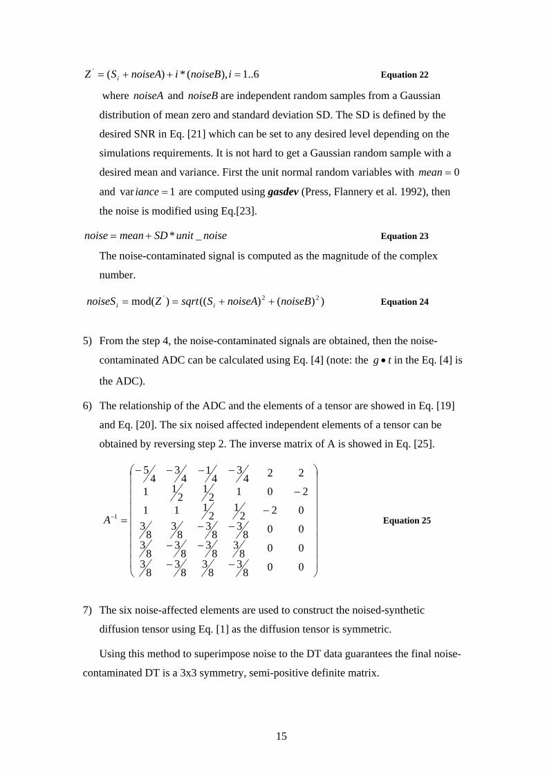
6) The relationship of the ADC and the elements of a tensor are showed in Eq. [19]
and Eq. [20]. The six noised affected independent elements of a tensor can be
obtained by reversing step 2. The inverse matrix of A is showed in Eq. [25].
⎟⎟⎟⎟⎟⎟⎟⎟⎟
⎠
⎞
⎜⎜⎜⎜⎜⎜⎜⎜⎜
⎝
⎛
−−
−−
−−−
−
−−−−
=−
0083
83
83
83
0083
83
83
83
0083
83
83
83
0221
2111
20121
211
2243
41
43
45
1A Equation 25
7) The six noise-affected elements are used to construct the noised-synthetic
diffusion tensor using Eq. [1] as the diffusion tensor is symmetric.
Using this method to superimpose noise to the DT data guarantees the final noise-
contaminated DT is a 3x3 symmetry, semi-positive definite matrix.
15

IMPLEMENTATION
The Streamlines, Tensorlines and TEND methods are tested using a synthetic
tensor filed with crossing fiber tracts with different levels of SNR. We first create a
synthetic tensor field with crossing fiber tracts, superimpose uniformly distributed
Gaussian noise with different levels of SNR to the tensor and integrate the fiber
pathways using Streamlines, Tensorlines and TEND techniques.
Construction of a Synthetic Tensor Field
The synthetic tensor fields we construct have 32x32x3 sample points. A B-Spline
space curve wrapped with a tube is used to present a synthetic fiber tract. The basic
idea is that tensors inside the tube are anisotropic; their eigenvectors are defined by
the Frenet-frame of the B-Spline space curve. On the other hand, the tensors outside
the tube are isotropic; their eigenvectors are random mutually orthogonal vectors. The
diffusion values of the isotropic tensor and anisotropic tensor are the following:
( ) ( )( ) ( )444
321
444321
10*4.010*5.210*7
10*310*310*3−−−
−−−
=
=
λλλ
λλλ
anisotropy
isotropy
T
T
The value’s units are smm2
(Lazar, Weinstein et al. 2003).
The Frenet-frame of a B-Spline curve is made of the tangent, normal and binormal
vectors. The tangent vector is computed by differentiating the parametric function of
the B-Spline curve. The normal vector is the cross production of the tangent vector
and the acceleration vector that is assumed normally to be a unit vector (0, 1, 0). If the
assumed acceleration vector is collinear to the tangent vector, it is reset to a unit
vector (1, 0, 0). The binormal vector is computed by taking the cross production of the
tangent and normal vectors after obtaining the tangent and normal vectors.
Each tensor in a 3D volume is tested if it is in the tube of the B-Spline by finding
the closet point on the B-Spline curve and computing the distance between the tensor
and the closet point. In this application the closest point is found using binary
searching the B-Spline curve which won’t cause ambiguity case as the B-Spline is
constructed to be smooth and low curvature (Figure 7).
16

Closest point Tube wrapping the curve
Tensor B-Spline
Figure 7: Finding closest point on the B-Spline curve using binary searching.
The synthetic tensor imaging with crossing fiber tracts is constructed by
combining two synthetic tensor fields with single fiber tracts in a way of averaging
their tensors in a region containing the crossing tracts. Figure 8 shows the crossing B-
Spline tubes and the synthetic tensor field constructed by the B-Spline tubes. It is
noticed that the tensors in the region containing crossing tracts are isotropic.
Figure 8: Right image shows the synthetic tensor fields constructed by the crossing tracts which are presented using two pink B-Spline tubes displayed in left image.
17

In the application, we also constructed a synthetic tensor field in which the fiber
tracts merge together (shown in Figure 9). For this tensor field, the tensors in the
region containing the merging tracts are anisotropic.
Figure 9: Right image shows the synthetic tensor fields with merging tracts which are presented using two pink B-Spline tubes displayed in left image.
To make the synthetic tensor field more realistic, Rician noise should be add to it
(Henkelman 1985; Gubjartsson and Patz 1995). In this application, Gaussian normal
noises are added to the tensor rather than Rician noise as the SNR level of the noises
are assumed greater than 3 (Jonasson, Hagmann et al. 2003).
Generating of noised-contaminated synthetic tensor fields
The procedure of adding Gaussian normal noises to the synthetic tensor field is
strictly followed the seven steps depicted in the previous section of “Simulation
procedure of adding noise to synthetic tensor field”. The noises with SNR of level 8,
16, 32, 64 …100000 are superimposed to the tensor field to test the fiber tracking
algorithms. Figure 10 shows the results of adding Gaussian normal noises with
different levels of SNR to the synthetic tensor field containing crossing fiber tracts.
18

Figure 10: Noised-contaminated synthetic tensor fields with the geometry of crossing fiber tracts with different level of SNR.
Simulations of fiber tracks
Streamlines, Tensorlines and Tensor Deflection (TEND) with Mid-point and RK-
4 integration methods are implemented and tested on the noised-affected synthetic
tensor fields with crossing fiber tracts with different levels of SNR. The simulations
start with choosing seed points for propagating observed fiber tracts. For each fiber
tractoraphy method, each tensor is test if it meets the seed point’s criteria. For instant,
if the tensor’s anisotropy is greater than 0.6 in the application, then it is a seed point.
19

After determining the seed point, two simulated tracts are issued from the seed point’s
center with a little offsets on XYZ directions. The two tracts extend along with the
positive direction and negative direction as is not able to verify if the
pathway is afferent or efferent. The simulation is terminated when the integration of
fiber tracts into a region where the tensors’ anisotropy is less than 0.2.
1e 1e 1e
On each step of computing the outgoing vectors of the local tensors from the
incoming vectors obtained from previous simulation step, the of the local tensors
are test first with the incoming vectors to see if the angle between them is less than
great than 90 degree. If the angle is, then the should be flipped, hence the outgoing
vectors are calculated based on the flipped .
1e
1e
1e
The main goal of the simulations is to test which fiber tracking algorithm is
reliable and stable on the regions containing fiber tracts with complex geometries,
such as crossing, merging, branching. Figure 11 shows the simulation results. The
integrated pathways of the fiber tracts in the synthetic tensor fields are colored in
different colors which show the pathways’ orientation in 3D (actually in 2D as the
simulation results are only displayed on a XY plane). The pathways extending mainly
on X, Y, Z directions are colored in blue, red and magenta respectively, other
pathways are colored in yellow.
20
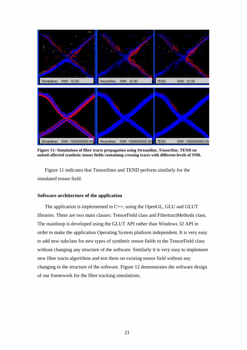
Figure 11: Simulations of fiber tracts propagation using Streamline, Tensorline, TEND on noised-affected synthetic tensor fields containing crossing tracts with different levels of SNR.
Figure 11 indicates that Tensorlines and TEND perform similarly for the
simulated tensor field.
Software architecture of the application
The application is implemented in C++, using the OpenGL, GLU and GLUT
libraries. There are two main classes: TensorField class and FibertractMethods class.
The mainloop is developed using the GLUT API rather than Windows 32 API in
order to make the application Operating System platform independent. It is very easy
to add new subclass for new types of synthetic tensor fields to the TensorField class
without changing any structure of the software. Similarly it is very easy to implement
new fiber tracts algorithms and test them on existing tensor field without any
changing to the structure of the software. Figure 12 demonstrates the software design
of our framework for the fiber tracking simulations.
21

Figure 12: Software architecture of the platform for the fiber tracts simulations.
User Guide
In the application, the mouse movements are used to rotate the rendered tensor
fields and the simulated fiber tracts around the center of the 3D space in a similar way
of rotating a 3D object in both hands. The following keys can be used to change
application settings:.
Key s/S: switch the rendering among
• Tensor field showed in ellipsoids with pathways simulated using
Streamline
• Colored pathways simulated using Streamline
• Tensor field showed in ellipsoids with pathways simulated using
Tensorline
• Colored pathways simulated using Tensorline
• Tensor field showed in ellipsoids with pathways simulated using TEND
• Colored pathways simulated using TEND
TensorField
Synthetic TensorField
Human Brain TensorField
Linear Synthetic TensorField
Crossing Synthetic TensorField
FibertractMethods
FibertractMethods
FibertractMethods
FibertractMethods
main
Is-A relationship Has-A relationship
22

• Ideal pathways of the synthetic tensor field showed tubes constructed by
B-Spline space curves.
Key w/W: increase/decrease the user-controlled parameter for Tensorline
simulations. The parameter varies from 0 to 1.
punctw
punctw
23

Error Measurements
The error of the three tract methods, Streamlines, Tensorlines, Tensor Deflection
(TEND) can be measured in three ways: 1. The average length of the simulated tracts;
2. The number of the tracts which follow the ideal tracts correctly; 3. The least square
error (LSE) of the simulated tracts. In the follow sections, SL stands for Streamline,
TL for Tensorlines in the charts and the tables.
Error Measurements of a Synthetic tensor field containing crossing tracts
The error measurements are done on the synthetic tensor field containing the
crossing fiber tracts which are described in Section “Implementation” and depicted in
Figure 8. First, we look at the changes of average length of the integrated tracts on the
synthetic tensor field with different levels of SNR without considering the tracts’
correctness.
Error measurements of the average length of the simulated tracts The average length is defined as a function of the minimum length which is the
integration condition for the simulation of the tracts. The whole length of the ideal
pathway in the synthetic tensor field is approximate 28 units.
Average Length (SNR=8)
0
24
6
810
12
1416
18
0 2 4 6 8 10 12 14 16
Min Length
Ave
rage
Len
gth
SL
TL
TEND
24

Average Length (SNR=16)
0
2
4
6
8
10
12
14
16
18
0 2 4 6 8 10 12 14 16 18
Min Length
Aver
age
Leng
th
SLTLTEND
Average Length (SNR=32)
0
5
10
15
20
25
0 5 10 15 20 25
Min Length
Aver
age
Leng
th
SLTLTEND
25

Average Length (SNR>1000000)
0
5
10
15
20
25
30
0 5 10 15 20 25 30
Min Length
Ave
rage
Len
gth
SLTLTEND
Figure 13: The changes of Average length of estimated tracts with levels of SNR ( 8, 16, 32 and over 1000000).
From the four charts rendered in Figure 13, it is obvious that TEND and
Tensorline generate much longer tracts than Streamline in the tensor filed with lower
SNR. At same situation, TEND is better than Tensorlines in terms of propagating
longer pathways.
When we study the white matter connectivity in vivo, the correctness of the tracts
are most important than other aspects, such as length, smoothness of the tracts. If the
simulated tracts can not represent the correct fiber tracts, it is pointless to study and
analyze such estimated tracts. Hence, another error measurement which has been done
in the application is measuring the number of correct tracts which follow the ideal
pathways which are constructed by using B-Spline space curves.
Error measurements of the correctness of the simulated tracts
A simulated tract is verified as correctly following the ideal pathway by testing
both of its end points inside the B-Spline tube which represent the ideal pathway.
Figure 14 includes 4 charts which demonstrate the changes of the number of the
correct tracts along with the minimum length on the synthetic tensor fields with
different levels of SNR. For example, the three methods can not propagate any
26

correct tracts when the minimum length that is the integration condition is increased
more than 13 units when the tensor field with SNR of 16.
Correctness of Simulated tracts (SNR=8)
0
5
10
15
20
25
30
35
40
0.0 1.0 2.0 3.0 4.0 5.0 6.0 7.0 8.0
Min Length
Num
ber o
f cor
rect
trac
ts
SLTLTEND
Correctness of Simulated tracts (SNR=16)
0
5
10
15
20
25
30
35
40
45
50
0.0 2.0 4.0 6.0 8.0 10.0 12.0 14.0
Min Length
Num
ber o
f cor
rect
trac
ts
SLTLTEND
27

Correctness of Simulated tracts (SNR=32)
0
10
20
30
40
50
60
70
0.0 5.0 10.0 15.0 20.0 25.0 30.0
Min Length
Num
ber o
f cor
rect
trac
ts
SLTLTEND
Correctness of Simulated tracts (SNR>1000000)
0
5
10
15
20
25
30
35
40
45
0.0 5.0 10.0 15.0 20.0 25.0 30.0
Min Length
Num
ber o
f cor
rect
trac
ts
SLTLTEND
Figure 14: Error measurement of correctness of tracts of a synthetic tensor field containing crossing fiber tracts.
We can see the three methods do not make much difference in generating correct
tracts when the synthetic tensor fields with lower SNR (such as 8, 16, and 32) from
the first three charts. When the SNR increases to almost an infinite number, the
synthetic tensor field is not affected by any noises, and the tensors are homogeneous
28
in all regions except the center where the two ideal pathways cross. In such situation,
Streamlines method can not generate any correct tracts when minimum length is
increased over half of the ideal pathway’s length. Though Streamline still propagates
longer and smooth tracts, all tracts deviate away from the right tracks when the
simulation enters into the region containing complex connectivity, such as tract
crossing, merging. On the other hand, Tensorlines and TEND methods do a much
better job than Streamline in such complex regions. Moreover, from the last chart of
Figure 14, TEND does a little bit better job than Tensorlines in terms of integrating
correct tracts.
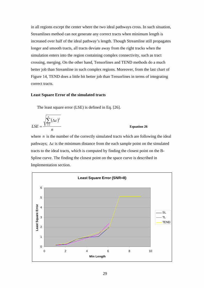
Least Square Error of the simulated tracts
The least square error (LSE) is defined in Eq. [26].
( )
nLSE
n
i∑=
∆= 1
2ε Equation 26
where is the number of the correctly simulated tracts which are following the ideal
pathways;
n
ε∆ is the minimum distance from the each sample point on the simulated
tracts to the ideal tracts, which is computed by finding the closest point on the B-
Spline curve. The finding the closest point on the space curve is described in
Implementation section.
Least Square Error (SNR=8)
0
1
2
3
4
5
6
0 2 4 6 8 10
Min Length
Leas
t Squ
are
Erro
r
SLTLTEND
29

Least Square Error (SNR=16)
0
0.5
1
1.5
2
2.5
0 2 4 6 8 10 12 14
Min Length
Leas
t Squ
are
Erro
r
SLTLTEND
Least Square Error (SNR=32)
0
0.2
0.4
0.6
0.8
1
1.2
1.4
1.6
1.8
2
0 2 4 6 8 10 12 14 16 18
Min Length
Leas
t Squ
are
Erro
r
SLTLTEND
30

Least Square Error (SNR>1000000)
0
0.5
1
1.5
2
2.5
3
3.5
4
0 5 10 15 20 25 30
Min Length
Leas
t Squ
are
Erro
r
SLTLTEND
Figure 15: The Least Square Error of the simulated tracts.
The first three graphs in Figure 15 indicate that the three methods do not make
much difference when the tensor fields with lower levels of SNR and the minimum
length is set to a small number. The last graph shows that on the synthetic tensor field
with higher levels of SNR that is great than 1000000, the simulated tracts generated
by using Tensorlines and the Tensor deflection methods have much more lower LSE
which keeps lower than 0.5, than the simulated tracts propagated by using Streamlines
which have much more bigger LSE which is never lower than 1. The last graph also
indicates that the TEND method does a little better job than the Tensorlines on such
synthetic tensor fields. The result is similar as the error measurement results of the
correctness of the tracts described in previous section.
Error Measurements of a Synthetic tensor field containing merging tracts
The error measurements are also done on the synthetic tensor fields containing the
merging fiber tracts which are described in Section “Implementation” and depicted in
Figure 9. Similarly as the error measurement done on the synthetic tensor fields
containing crossing fiber tracts, first we exam the changes of average length of the
integrated tracts on the synthetic tensor field with different levels of SNR without
considering the tracts’ correctness, then test the correctness of the tracts, finally exam
31

the Least Square Error of the simulated tracts. The whole length of the ideal pathway
in the field is about 29 units.
Error measurements of the average length of the simulated tracts
The error measurements are presented in graphs.
Average Length (SNR=8)
0
2
4
6
8
10
12
14
16
18
0 5 10 15 20
Min Length
Aver
age
Leng
th
SLTLTEND
Average Length (SNR=16)
0
5
10
15
20
25
0 5 10 15 20 25
Min Length
Ave
rage
Len
gth
SL
TL
TEND
32

Average Length (SNR=32)
0
5
10
15
20
25
30
0 5 10 15 20 25 30
Min Length
Aver
age
Leng
th
SLTLTEND
Average Length (SNR>100000)
0
5
10
15
20
25
30
0 5 10 15 20 25 30
Min Length
Aver
age
Leng
th
SLTLTEND
Figure 16: The changes of Average length of estimated tracts with levels of SNR ( 8, 16, 32 and over 1000000).
From the first two charts in Figure 15, The Tensorlines algorithm generates longer
simulated tracts than Streamlines and TEND methods do when the tensor fields with
lower levels of SNR. In order to see the difference among the Streamlines,
Tensorlines and TEND methods in the last chart in the Figure 15, Table 1 shows the
33

dataset which is depicted in the last chart. From the last two charts and the Table 1,
we can see that when the levels of SNR of the tensor fields become to 32 and over 32,
the three methods have quiet similar results.
Table 1: The average length over the min length (SNR>1000000)
minLength SL TL TEND minLength SL TL TEND 1.1 21.8241 22.4662 22.4921 14.1 27.7164 28.0264 28.0323 2.1 22.5336 23.1963 23.2232 15.1 27.9353 28.0264 28.0323 3.1 23.0103 23.4407 23.4679 16.1 27.9353 28.0264 28.0323 4.1 23.2411 23.674 23.7014 17.1 27.9353 28.2072 28.2132 5.1 23.7014 24.1454 24.1735 18.1 28.1023 28.2072 28.2132 6.1 23.9339 24.3732 24.4017 19.1 28.4495 28.3745 28.3793 7.1 23.9339 24.3732 24.4017 20.1 28.4495 28.3745 28.3793 8.1 24.1392 24.7963 24.8255 21.1 28.4495 28.3745 28.3793 9.1 24.5376 25.4404 25.4708 22.1 28.4495 28.3745 28.3793
10.1 24.7304 25.4404 25.4708 23.1 28.4495 28.3745 28.3793 11.1 24.9148 25.8418 25.873 24.1 28.4495 28.3745 28.3793 12.1 27.273 26.0375 25.873 25.1 28.4495 28.3745 28.3793 13.1 27.273 26.0375 25.873 26.1 28.4495 28.429 28.4339
Error measurements of the correctness of the simulated tracts Then three methods are tested in term of generating the correct tracts which are
following the ideal pathways. The datasets obtained from the error measurement
employed on the synthetic tensor fields with different levels of SNR are listed in
Table 2 to Table 5 rather than graphs as it is hard to see the difference from graphs. Table 2: Number of the correct tracts over the min length (SNR=8)
minLength SL TL TEND minLength SL TL TEND 1.1 29 25 28 6.1 0 1 1 2.1 17 14 13 7.1 0 1 1 3.1 8 9 7 8.1 0 1 0 4.1 3 6 4 9.1 0 0 0 5.1 1 3 2
Table 3: Number of the correct tracts over the min length (SNR=16)
minLength SL TL TEND minLength SL TL TEND 1.1 37 36 35 7.1 2 2 3 2.1 24 25 23 8.1 1 1 1 3.1 13 15 12 9.1 1 1 1 4.1 9 11 9 10.1 1 1 1 5.1 3 5 4 11.1 0 0 0 6.1 3 5 4
34

Table 4: Number of the correct tracts over the min length (SNR=32)
minLength SL TL TEND minLength SL TL TEND 1.1 40 44 41 14.1 3 3 3 2.1 31 35 33 15.1 3 3 3 3.1 23 26 24 16.1 3 3 3 4.1 16 19 18 17.1 3 3 3 5.1 12 14 16 18.1 3 3 3 6.1 11 13 12 19.1 3 3 3 7.1 8 9 9 20.1 3 3 3 8.1 7 9 9 21.1 3 3 3 9.1 5 6 6 22.1 3 3 3
10.1 4 4 5 23.1 2 2 2 11.1 3 3 3 24.1 2 2 2 12.1 3 3 3 25.1 1 2 2 13.1 3 3 3 26.1 0 2 1
Table 5: Number of the correct tracts over the min length (SNR>1000000)
minLength SL TL TEND minLength SL TL TEND 1.1 61 60 60 14.1 55 55 55 2.1 61 60 60 15.1 54 55 55 3.1 61 60 60 16.1 54 55 55 4.1 61 60 60 17.1 54 54 54 5.1 61 60 60 18.1 54 54 54 6.1 61 59 59 19.1 54 54 54 7.1 61 59 59 20.1 54 54 54 8.1 60 58 58 21.1 54 54 54 9.1 58 57 57 22.1 54 54 54
10.1 57 57 57 23.1 54 54 54 11.1 56 55 55 24.1 54 54 54 12.1 55 55 55 25.1 54 54 54 13.1 55 55 55 26.1 54 53 53
When SNR is lower and minimum length is smaller, Tensorlines and TEND
methods do a little bit better job than Streamlines algorithm. However the results of
the error measurement for the three methods are very similar when the value of the
SNR of the synthetic tensor fields is higher than 1000000. This is different from the
same error measurements done to the synthetic tensor fields with geometry of
crossing tracts, which are described in previous section. This is because the synthetic
tensor fields (Figure 9) containing merging tracts with high level of SNR almost are
anisotropic in the regions containing the fiber tracts which merge together to be a
single bundle of tracts, and the synthetic tensor fields (Figure 8) containing the
crossing tracts with whatever level of SNR are not anisotropic in the region where two
tracts cross each other.
35

Least Square Error of the simulated tracts The LSE is computed using Eq. 26 and the results of the error measurement are
presented in tables rather than graphs as the differences of the three methods are not
obvious to be seen in graphs.
Table 6: Least Square Error (SNR=8)
minLength SL TL TEND minLength SL TL TEND 1.1 0.187352 0.228236 0.228929 5.1 1.15345 1.05002 1.266142.1 0.245145 0.339293 0.416951 6.1 Not valid 2.69748 2.306863.1 0.401325 0.476245 0.512679 7.1 Not valid 2.69748 2.306864.1 0.852262 0.635407 0.758163 8.1 Not valid 2.69748 Not valid
Table 7: Least Square Error (SNR=16)
minLength SL TL TEND minLength SL TL TEND 1.1 0.150924 0.150036 0.153241 6.1 0.891907 0.607536 0.8130952.1 0.207892 0.192014 0.207385 7.1 1.26167 1.13778 1.053.1 0.339747 0.285552 0.344629 8.1 0.510967 0.564326 0.5191664.1 0.430911 0.348086 0.427186 9.1 0.510967 0.564326 0.5191665.1 0.891907 0.607536 0.813095 10.1 0.510967 0.564326 0.519166
Table 8: Least Square Error (SNR=32)
minLength SL TL TEND minLength SL TL TEND 1.1 0.167134 0.173625 0.181884 14.1 1.47771 1.58867 1.646942.1 0.207339 0.205514 0.218633 15.1 1.47771 1.58867 1.646943.1 0.26786 0.268389 0.290786 16.1 1.47771 1.58867 1.646944.1 0.356267 0.339106 0.356317 17.1 1.47771 1.58867 1.646945.1 0.44814 0.426445 0.381744 18.1 1.47771 1.58867 1.646946.1 0.488404 0.45886 0.506477 19.1 1.47771 1.58867 1.646947.1 0.629796 0.638573 0.654455 20.1 1.47771 1.58867 1.646948.1 0.695319 0.638573 0.654455 21.1 1.47771 1.58867 1.646949.1 0.966629 0.90241 0.955252 22.1 1.47771 1.58867 1.64694
10.1 1.20334 1.28251 1.14289 23.1 1.13969 1.14511 1.120211.1 1.47771 1.58867 1.64694 24.1 1.13969 1.14511 1.120212.1 1.47771 1.58867 1.64694 25.1 1.67759 1.14511 1.120213.1 1.47771 1.58867 1.64694 26.1 Not valid 1.14511 1.60319
Table 9: Least Square Error (SNR>1000000)
minLength SL TL TEND minLength SL TL TEND 1.1 0.235111 0.234524 0.235674 14.1 0.213207 0.215855 0.2172512.1 0.235111 0.234524 0.235674 15.1 0.207818 0.215855 0.2172513.1 0.235111 0.234524 0.235674 16.1 0.207818 0.215855 0.2172514.1 0.235111 0.234524 0.235674 17.1 0.207818 0.216664 0.2181365.1 0.235111 0.234524 0.235674 18.1 0.207818 0.216664 0.2181366.1 0.235111 0.232685 0.233861 19.1 0.207818 0.216664 0.2181367.1 0.235111 0.232685 0.233861 20.1 0.207818 0.216664 0.2181368.1 0.235114 0.232242 0.233497 21.1 0.207818 0.216664 0.2181369.1 0.226538 0.226592 0.227823 22.1 0.207818 0.216664 0.218136
10.1 0.22454 0.226592 0.227823 23.1 0.207818 0.216664 0.21813611.1 0.218967 0.215855 0.217251 24.1 0.207818 0.216664 0.21813612.1 0.213207 0.215855 0.217251 25.1 0.207818 0.216664 0.21813613.1 0.213207 0.215855 0.217251 26.1 0.207818 0.209722 0.211252
36

From the datasets listed in Table 6-9, we can see that the three methods have very
similar results of the measurements of the Least Square Error. However, when the
synthetic tensor fields which contain merging tracts have high levels of SNR, the
simulated tracts generated by using Streamlines algorithm have smaller LSE than the
tracts generated by using Tensorlines and TEND methods. The results of the
measurement of LSE are similar as the results of the error measurement of the
correctness of tracts for the synthetic tensor fields with the geometry of merging tracts.
The results of the three error measurements are in accordance with the purpose of
the Tensorlines and Tensor Deflection methods, which are designed to deal with the
un-anisotropic tensors. In a anisotropic tensor field, the three methods should generate
similar tracts.
37

CONCLUSIONS
A platform is created to test fiber tracking algorithms on noise-affected synthetic
tensor fields. The platform is easy to be extended by adding new types of synthetic
tensor fields or new fiber tractography methods for testing. Due to time constraints,
we could stimulate and test only two fiber configurations. The error measurements in
terms of average length of the estimated tracts, the number of correct tracts and the
Least Square Error of tracts are analyzed on noise-contaminated synthetic fields
containing crossing tracts and merging tracts with different levels of SNR respectively.
The limit results of error measurements indicate Tensorlines and TEND are more
suitable for inhomogeneous tensor fields than Streamline.
The three methods are not tested on linear or radiant homogeneous tensor fields in
this project as Lazar and Alexander have done it in 2003(Lazar and Alexander 2003).
More testing has to be done to obtain a better understanding of the advantage and
disadvantage of the three fiber tracking methods. And also, more fiber tractography
methods should be tested, such as Markov chain algorithm.
When adding noises to the synthetic tensor in the project, the B-factor is assumed
to 21000 mmsb = simply. The value may not be suitable for inhomogeneous tensors
containing more complex fiber connectivity. The effect of choosing of B-factor
should be considered when constructing synthetic tensor fields for testing fiber
tractography methods.
38

ACKNOWLEDGEMENTS
Many thanks to Burkhard for his supervision on the project. I greatly appreciated
the help from Lisa Jonasson, Donald Tournier and Peter Basser who answered my
questions promptly and clearly and sent me the papers that I could not find on the
internet. Without their help, I doubt I could finish the work.
REFERENCES Basser, P. J., S. Pajevic, et al. (2000). "In vivo fiber tractography using DT-MRI data." Magnetic Resonance in Medicine 44(4): 625-632. Gubjartsson, H. and S. Patz (1995). "The Rician distribution of noisy MRI data." Magn Reson Med 34: 910-914. Henkelman, R. (1985). "Measurement of signal intensity in the presence of noise in MR images." Med Phys 12: 232-233. Hesselink, L., Y. Levy, et al. (1997). "The topology of symmetric, second-order 3D tensor fields." IEEE Transactions on Visualization and Computer Graphics 3(1): 1-11. Jonasson, L., X. Bresson, et al. (2005). "White matter fiber tract segmentation in DT-MRI using geometric flows." Medical Image Analysis 9(3): 223-236. Jonasson, L., P. Hagmann, et al. (2003). White Matter Mapping in DT-MRI using geometric flows. 9th International Conference on Computer Aided Systems Theory, Las Palmas de Gran Canaria, Spain. Lazar, M. and A. L. Alexander (2003). "An error analysis of white matter tractography methods: synthetic diffusion tensor field simulations." Neuroimage 20: 1140-1153. Lazar, M., D. M. Weinstein, et al. (2003). "White matter tractography using diffusion tensor deflection." Human Brain Mapping 18(4): 306-321. Mori, S. and P. C. M. v. Zijl (2002). Fiber tracking: principles and strategies - a technical review. NMR in Blomedicine. 15: 468-480. Papadakis, N. G., D. Xing, et al. (1999). "A Comparative Study of Acquisition Schemes for Diffusion Tensor Imaging Using MRI." Journal of Magnetic Resonance 137: 67-82. Pierpaoli, C., P. Jezzard, et al. (1996). "Diffusion tensor MR imaging of the human brain." Radiology 201(3): 637-648.
39

Press, W. H., B. P. Flannery, et al. (1992). Numerical Recipes in C: The Art of Scientific Computing. Cambridge, Cambridge University Press. Shahar, A. R. B. "The Human Brain." http://www.imt.co.il/humanbrain.htm. Skare, S., T.-Q. Li, et al. (2000). "Noise consideraions in the determination of diffusion tensor anisotropy." Magnetic Resonance Imaging 18(6): 659-669. Tuch, D. S. (2004). "Q-Ball Imaging." Magnetic Resonance in Medicine 52: 1358-1372. Weinstein, D. M., G. Kindlmann, et al. (1999). Tensorlines: Advection-diffusion based propagation through diffusion tensor fields. Proceedings of Visualization. Westin, C.-F., S. E. Maier, et al. (1999). Image processing for diffusion tensor magnetic resonance imageing. Medical Image Computing and Computer-Assisted Intervention, Cambridge, UK, Springer Verlag. Westin, C.-F., S. Peled, et al. (1997). Geometrical diffusion measures for MRI from tensor basis analysis. Proceeding of ISMRM. Wuensche, B. (2004). Visualization Techniques for Vector Fields. Comupter Science 716 lecture notes, The university of auckland (http://www.cs.auckland.ac.nz/compsci716s2t/lectures/). Wuensche, B. and R. Lobb (2003). The 3D visualization of brain anatomy from diffusion-weighted magnetic resonance imaging data. Computer graphics and interactive techniques in Australasia and South East Asia. Young, E. C. (1993). Vector and Tensor Analysis, Marcel Dekker, Inc.
40