April 1990 LIDS-P-1967

An Alternating Direction Method for Linear Programming*

by

Jonathan ECKSTEINGraduate School of Business, Harvard UniversityBoston, MA 02163

Dimitri P. BERTSEKASLaboratory for Information and Decision Systems, Massachusetts Institute of TechnologyCambridge, MA 02139

Abstract

This paper presents a new, simple, massively parallel algorithm for linear programming,called the alternating step method. The algorithm is unusual in that it does not maintainprimal feasibility, dual feasibility, or complementary slackness; rather, all these conditions aregradually met as the method proceeds. We derive the algorithm from an extension of thealternating direction method of multipliers for convex programming, giving a new algorithm formonotropic programming in the course of the development. Concentrating on the linearprogramming case, we give a proof that, under a simple condition on the algorithmparameters, the method converges at a globally linear rate. Finally, we give somepreliminary computational results.

Key Words: Linear programming, parallel algorithms, proximal point algorithms,monotropic programming

Abbreviated Title for Running Heads: An Alternating Direction Method

* This paper consists mainly of refinements of dissertation research results of the first author.The dissertation was performed at M.I.T. under the supervision of the second author, andwas supported in part by the Army Research Office under grant number DAAL03-86-K-0171,and by the National Science Foundation under grant number ECS-8519058. Alliant FX/8computer time was donated by the Mathematics and Computer Science division of ArgonneNational Laboratories.

-1-

1. Introduction

This paper develops the alternating step method, a novel, simple algorithm for linear

programming that is very amenable to parallel implementation. This algorithm works by

applying simple linear updates alternately to the primal and dual variables of the linear

program (hence its name), but is unusual in that it does not enforce primal feasibility, dual

feasibility, or complementary slackness. Instead, all these properties are gradually satisfied

as the algorithm progresses. Simplex and dual relaxation methods for linear programming

generally enforce two of these properties, while working to satisfy the third; even interior

point methods generally enforce feasibility restrictions.

The alternating step method is original to the authors; however, a preliminary derivation

appears in Bertsekas and Tsitsiklis (1989, p. 254). The more thorough analysis presented

here is a refinement of that of Eckstein (1989).

We derive the alternating step method by specializing the generalized alternating direction

method of multipliers, a decomposition algorithm for convex programming (Eckstein and

Bertsekas 1989). This algorithm is presented in Section 2, and is an extension of the earlier

alternating direction method of multipliers, which was first introduced by Glowinski and

Marroco (1975), and by Gabay and Mercier (1976). Further contributions to the theory of the

alternating direction method of multipliers appeared in Fortin and Glowinski (1983), and

Gabay (1983). Glowinski and Le Tallec (1987) give an extensive treatment of the method

and its relatives, and a relatively accessible exposition appears in Bertsekas and Tsitsiklis

(1989, pp. 253-261). However, an intimate understanding of the workings of these

alternating direction methods is not necessary for the majority of this paper.

Section 3 uses the generalized alternating direction method of multipliers to derive the

alternating step method for monotropic programming, that is, linearly-constrained convex

programming with a separable objective (Rockafellar 1984), while Section 4 then specializes

-2 -

this algorithm to the case of linear programming. Related work in the literature includes

Spingarn's (1985b) application of the method of partial inverses to optimization, in particular

the algorithm for block-separable convex programming. Gol'shtein's "block" method of convex

programming (1985, 1986) are based on a fundamentally identical decomposition strategy.

The theoretical underpinnings relating the Spingarn and Gol'shtein convex programming

algorithms to the alternating direction method of multipliers are elaborated in Eckstein and

Bertsekas (1989) and Eckstein (1989), where additional references are given. A distin-

guishing feature of our approach is that we apply a dimension-increasing transformation to the

original monotropic program, increasing the number of variables from n to nm, where m is the

number of constraints. After deriving an algorithm for this expanded problem, we simplify it

until it involves only primal variables of dimension n and dual variables of dimension m. We

should also note that there have been numerous applications of the conventional (as opposed

to alternating direction) method of multipliers to linear programming. For one example,

consider De Leone and Mangasarian (1988).

Section 5 gives a proof that, under a simple condition on the algorithm parameters, the

alternating step method for linear programs converges at a globally linear rate. The analysis

draws on ideas from the convergence analysis of the proximal point algorithm (Luque 1984),

and results in linear programming stability theory (Mangasarian and Shiau 1987). Similar

preceeding work on convergence rates includes the asymptotic convergence rate result for

Spingarn's block-separable convex programming method (1985b, Section 4); however, that

analysis makes the rather stringent assumption that the problem meets the strong second-

order sufficiency conditions. Here, we make only the assumptions that the linear program in

question is feasible with bounded objective value. Our result is closer in spirit to Spingarn's

(1985a, 1987) finite termination and asymptotic convergence rate results concerning his

partial-inverse-based methods for linear inequality systems. These methods could in

principle be applied to linear programming by posing the primal and dual problems as a single

system of inequalities. However, we prove convergence at a global, as opposed to

asymptotic, linear rate. Because of the complexity of the analysis, Section 5 assumes

-3-

familiarity with the theory of the generalized alternating direction method of multipliers, and

the proximal point algorithm that underlies it (Eckstein and Bertsekas 1989, Lawrence and

Spingarn 1987, Eckstein 1988, Eckstein 1989). It is the only part of this paper that requires

such familiarity.

Section 6 gives preliminary computational results for the method, and describes some simple

heuristics that accelerate its convergence in practice. For general linear programming, the

method appears to be uncompetitive in a serial computing environmnet. Taking advantage of

parallelism and certain specialized constraint structures, however, the method does show

some promise. Versions of the method have been implemented on a variety of parallel

computers; details of these implementations are reserved for a future paper.

2. The Generalized Alternating Direction Method of Multipliers

We now present the generalized alternating direction method of multipliers, upon which our

derivation is based. For background material on convex analysis, see Rockafellar (1970).

First, consider a general finite-dimensional optimization problem of the form

minimize xEn fix) + g(Mx) , (P)

where f: R1n - (- oo, + oo] and g: Rs ---> (- o, + oo] are closed proper convex, and M is some

s x n matrix. One can also write (P) is the form

minimize fAx) + g(z) (P')subject to Mx = z ,

and attaching a multiplier vector p E R s to the constraints Mx = w, one obtains an equivalent

dual problem

maximize ps -f*(-MTp) + g*(p)) , (D)

where * denotes the convex conjugacy operation. The alternating direction method of

multipliers for (P) takes the form

-4-

xk+l = arg min {fix) + (pk, Mx) + 1I Mx - zk112}

zk+l = arg min {g(z) - (pk, z) + 2 II MXk+l _ Z112}

pk+l = pk + (Mxk+l _ zk+l)

where A is a given positive scalar. This method resembles the conventional Hestenes-

Powell method of multipliers for (P') (e.g. Bertsekas 1982), except that it minimizes the

augmented Lagrangian function

LA(x, z, p) = f(x) + g(z) + (pk, Mx - Z) + 2 II Mx - Z112

first with respect to x, and then with respect to z, rather than with respect to both x and z

simultaneously.

A pair (x, p) E R n x Rs is said to be a Kuhn-Tucker pair for (P) if -MTp E af(x) and p E

ag(Mx), where a denotes the subgradient mapping, as in Rockafellar (1970). It is a basic

exercise in convex analysis to show that if (x, p) is a Kuhn-Tucker pair, then x is optimal for

(P), p is optimal for (D), and the two problems have an identical, finite optimum value. We

now present the generalized alternating direction method of multipliers:

Theorem 1 (The generalized alternating direction method of multipliers). Consider a convex

program in the form (P), minimize x E lRn Jx) + g(Mx), where M has full column rank. Let pO,

ZO E Rm, and suppose we are given some scalar X > 0 and

00

{k}k'=O C [0, 00), Lk < 00k=O

{Vk}k=0 [0, oo), Vk 00k=O

{Pk}k= 0 C (0, 2) 0 < inf Pk < suppk < 2k O k>0

-5-

Suppose {xk}k= 1, {zk}k= 0 , and {pk}k= 0 conform, for all k, to

IIxk+ _ arg min {J(x) + (pk, Mx) + 11 Mx - zk 112} II < Ik

I zkl - arg min {g(z) - (pk, z) + 1 pkMx k +l + (1 - pk)zk - z 112} 1 < Vk

pk+l = pk + X(pkMxk+l + (1 - pk)zk - zk+l)

Then if (P) has a Kuhn-Tucker pair, {xk} converges to a solution of (P) and {pk} converges to

a solution of the dual problem (D). Furthermore, {zk} converges to Mx*, where x* is the

limit of {xk}. If (D) has no optimal solution, then at least one of the sequences {pk} or {zk}

is unbounded.

The proof of this theorem is given in Eckstein and Bertsekas (1989), and is based on an

equivalence to an extension of the proximal point algorithm. Basically, the generalized

alternating direction method of multipliers reduces to the alternating direction method of

multipliers is the special case that Pk = 1 for all k > 0, but also allows for approximate

minimization of the augmented Lagrangian.

3. Monotropic Programming

A monotropic program (Rockafellar 1984) is an optimization problem taking the canonical

form

nminimize E hj(xj)

(MP)subject to Ax = b

X En ,

where the hj: R ~ (-oo, + oo], j=l,...,n, are closed proper convex, A is a real m x n matrix, and

b E -6-m.

-6-

Since the hi can take on the value +oo, they may contain implicit constraints of the form xj > Ij

Ei R and xj < uj E- R. Thus, by proper choice of the hj and the familiar device of slack

variables, any convex optimization problem with a separable lower semicontinuous objective

and subject to a finite number of linear equality and inequality constraints can be converted to

the form (MP).

Given a monotropic program (MP), define d(i), the degree of constraint i, to be the number of

nonzero elements in row i of A. If A is the node-arc incidence matrix of a network or graph,

then this definition agrees with the usual notion of the degree of node i. Let aj denote column

j of A, 1 <j < n, and let Ai denote row i of A, 1 < i < m.

The surplus or residual ri(x) of constraint i of the system Ax = b, with respect to the primal

variables x, is bi - (Ai, x). Intuitively, ri(x) is the amount by which the ith constraint of the

system Ax = b is violated. Let r(x) denote the vector b - Ax of all m surpluses.

Let Qi, for 1 < i < m, be any set such that

{j I l<j<n, aij O} c_ Qi c {l,...,n}

Let qi = IQil for all i, hence d(i) < qi < n. Furthermore, let

Q= {(i,j) I < i < m,j E Qi}

We now convert (MP) to the form (P), minimize Ax) + g(Mx). Here, f will be defined on 1 n

and g on Rmn. Index the components of vectors z E pmn as zij, where 1 < i •< m and 1 < j < n.

Then let

n

f(x)= hj(xj)j=1

-7-

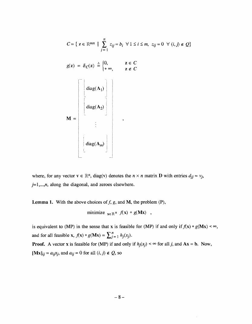
nC= { z E Rm n I z,= V I _< i < m, zij = O V (i,j) Q}

i=l

AJO, zE Cg(z) = C(Z) - + zX C

diag(Al)

diag(A 2)

M=

diag( Al)

where, for any vector v E kn, diag(v) denotes the n x n matrix D with entries djj = vj,

j=l,...,n, along the diagonal, and zeroes elsewhere.

Lemma 1. With the above choices off, g, and M, the problem (P),

minimize xRn f(x) + g(Mx) ,

is equivalent to (MP) in the sense that x is feasible for (MP) if and only if Ax) + g(Mx) < o,

and for all feasible x, fAx) + g(Mx) = =1 hj(xj).

Proof. A vector x is feasible for (MP) if and only if hj(xj) < M for all j, and Ax = b. Now,

[Mx]ij = aijxj, and aij = 0 for all (i, j) t Q, so

-8-

0 J X aijxj=bi V i, aijxj =O V(i,j) Q

g(Mx) - j=1

+ oo, otherwise

_ 10 , Ax=b- + oo ,otherwise

Thus, JAx) + g(Mx) is finite if and only if x is feasible for (MP), establishing the first claim.

For the second claim, note that x being feasible implies g(Mx) = 0, hence AJx) + g(Mx) = Afx)

= n=lhj(xj). ·

Lemma 2. Unless A has a column that consists entirely of zeroes, the matrix M defined

above has full column rank.

Proof. Let x E Rn be such that Mx = 0. Then aijxj = 0 for all i and j. As A is supposed to

have no zero columns, there exists, for every j, an i(j) E { 1,..., m} such that aiCe)j O. It

follows that xj = 0 for all j, and that x is the zero vector. ·

For any z E Rmn, and 1 < i < m, let zi E En be the subvector of z with components z ij,

j=l,...,n. Let

nCi ={zie Rn I A zij=b, z ij =O Vj Qi } ,

j=1

so that C= C 1 x ... x Cm.

We now apply the genernalize alternating direction method of multipliers to this formulation.

We let vk = 0 for all k, so that the method reduce to

-9-

Choose xk+l: II xk+l - arg min {f(x) + (pk, Mx) + 5- 11 Mx - zk 1121} ! < kx

zk+l = arg min {g(z) - (pk, z) + A 11 pkMxk+l + (1 - pk)zk - z 1121

pk+l = pk + 2.(pkMxk+l + (1 - pk)zk - zk+l)

Consider first the task of choosing xk+l. By the separability off and the form of M, this

problem can be decomposed into n independent tasks of the form

Choose xk+1' xk+l- arg min (x)+ai + (a -) 2 < ek= I t:jEQi

where we let ek = n(-1/2)!uk. Now consider the computation of zk+l , which decomposes into

the m independent calculations

min n Zzk+l = arg min i 2 (Pkaijx+ + (- Pk)-zi i =l,

zi Ci j= 1

To solve this problem for each i, we attach a single Lagrange multiplier 7zk +l to the constraint

j =1 Zij = bi which defines Ci. At the optimum, the Karush/Kuhn-Tucker conditions give,

for all i and j such that j e Qi, that

n n k~l f1,~7.\5r k 2\ _ '-(l, Zi) + /k+l(bi-= zij) + (Pkaij (1- =

Ozij) j 1 j =Pk 1 t

Equivalently,

Pijk - ik +l + ((zij- kaijxjk+l-(l -pk)zijk) = 0 tVE Qi

and so we obtain that

Pkaijx+ + (1- Pk)z Pzk+l _

i0 -

-10-

We determine the values of the 7rk+ l by setting, for each i,

/ =1 k+l =z) ·pkk( 1 £ al(j=l j Qi jE Qi jE Qi

For all k 2> 1, 1 j E Q z k = b i by construction. Assume that z0 is chosen so that

ji e i ZO = b i for all i. Then, for all k, we can simplify the above equation to

Pkbi = Pk aijx+l 1+ ( k + c/k+l)

jE Qi je Qi

Solving for 7rk+ and using the definition of ri(x),

Xk+l = (i Pkri(xk+l) -_ pk

j =- QJ

The final step in the generalized alternating direction method of multipliers iteration is the

update of the multipliers p, which takes the form

pk+1 = pk + 2(pkMxk+l + (1 - pk)zk - zk+l)

For (i, j) e Q, this multiplier update formula implies pk.+l = pik. For (i, J) E Q, we have

pk+l= pk + 1(Pkai x+l + (1 - Pk) k + 1)

=pk+x( 1 [pk+ rk+ 1)

-= _ k+l

Thus the Pijk+l, (i, j) E Q, do not vary with j. This is no coincidence, but is a natural

consequence of the structure of g and the monotone operator splitting method underlying the

generalized alternating direction method of multipliers (Eckstein 1989).

Now assume that p0 is such that for some no E ] m, Pii? = - T0 for all (i, j) E Q. It then

follows Pik = - 7cik for all k > 0 and (i, J) E Q. Noting that the values of the poi, (i, j) X Q, are

inconsequential, one can then substitute - 7ik for pi-k everywhere, and obtain the overall

method

Choosexl x'+ : x+l- arg min hj(xj) -(aj, k)xj + :j (a- zi i < e kChoose X) - 1 khi(xi) [k 2. 2u Ek

Irk+ 1 k + XPk ri(xk+ 1)qi

(Pzak+l + ( Pk) - ri(xk+l), (i,j) Qk+1 - Pk zk

zkl -l ~ 0 , (ij) O Q

Just as the sequence of mn-dimensional multipliers {pk} can be replaced by the m-

dimensional sequence {Ik}, the variables {zk} c_ Rmn can be replaced by a sequence {yk} c

1n, as follows:

Lemma 3. Assume that z0 is of the form

o Jaiy - ri(O), (i, j) Q

zi -0, (i,j) 0 Q

for some y°0 E Wn. Define the sequence {yk} via the recursion

yk+l = (1_pk)yk + pkxk +l Vk>O

Then

z = aijk ri(yk) V (i,j) , k O 0

Proof. The statement holds by hypothesis for k = 0. Assuming it holds for k, we have, for all

(i,j) e Q,

aijyjk+l _- ri(yk+1)

= aij((l -k) k + Pk X k+ l ))- (bi - (Ai, yk+l))

= (1 - pk)aijyJk + pkaijxjk+l - 1 ((1 - Pk)(bi - (Ai, yk)) + pk(bi - (Ai, xk+l)))

-12-

= (1 - k)[aijyj- ri(k)] + aijx +1 k ri(xk+l)

= (1 - k)Zik + Pkaijxjk +l - Pk ri(xk+l)

k+1

So, the claim holds by induction. A

Under the assumptions of Lemma 3, one can eliminate the zij and use that (i, j) o Q implies

aij = 0, obtaining

xk+l - arg min 'h.(xj) - (ajk)xj + 2 (aijxj -(aj)y + Ikri(Yk)))2 <kX -Xi j 2i:jeQ Ek

k+l = rk + X ri(xk+1)

k+l = (1 - Pk)Y + + PkX k +1

Collecting terms in the squared expressions, we obtain the alternating step method for

monotropic programming:

k X h1(x1) 2 1 __xjk+al ma m!rg m in ,hjxj ) +- (ASMP)

+=rk + iqtk ri(xk+l)

yk+l = (1 p -k)yk + pkxk +l ,

where yO E Rkn and sO0 E Rm are completely arbitrary. Note that there is no longer any direct

reference to the sets Q or Qi. We merely allow qi to be any integer between d(i) and n,

inclusive. In the degenerate case that d(i)=O for some i, we must require that qi be at least 1

so that (ASMP) remains well-defined. In practice, any such constraints of degree zero can be

immediately eliminated from the problem.

-13-

In the special case that Pk = 1 for all k, the sequences {xk} and {yk}, are identical, and the

method can be expressed

llaj112 nIx k maijri(xk)21tXf +1 =arg min hj(xj) -(aj, k)xj + 2 (iXj X ! 1 k)

(,k + 1= ( K+ q ri(x)k+ 1)I i qi

We use the term alternating step method because, in this form, the algorithm makes alternate

updates to the variables x of (MP) and those of its dual (Rockafellar 1984, Chapter 11A)

n

minimize ,,m h/*(aJ) - bTaj=1

where hj* denotes the convex conjugate of hj.

The updates of the primal variables xj and yj are completely independent over j, and the

updates of the dual variables 7ri are likewise independent over i. Thus, the method has the

potential for massive parallelism.

We now seek to apply Theorem 1 to show that (ASMP) converges. Theorem 1 requires the

existence of a Kuhn-Tucker pair, so we address this issue first. For any j, we say that hi is

pseudopolyhedral if

h) hi(x) , x E Vj

where hi is finite and convex throughout RI, and each Vj c R is a closed (but not necessarily

bounded) interval. For an explanation of this terminology, see Eckstein (1989), Section 3.5.1.

-14-

Lemma 4. If the hj are pseudopolyhedral for all j, then for the above definition off, g, and M,

(P) has a Kuhn-Tucker pair if and only if (MP) has a finite-valued optimal solution.

Proof. If (P) has a Kuhn-Tucker pair, then it has a finite optimal solution x*, and, by Lemma

1, x* must also be optimal for (MP). Conversely, suppose, that (MP) has a finite-valued

optimal solution x*. Then x* must be optimal for (P), and hence 0 E O[f + g o M](x*).

Writing f as f + BV, where

n

f(x) = i hj(xj)j=1

and

AVy() /0 xjE V j=l,...,n

\ + otherwis e,

we have that 6V and g o M are polyhedral functions, and, as (MP) is assumed to be feasible,

ri(dom fi n dom 3 v n dom(g o M)

= En (V1 x ... x Vn) n {x E Rn I Ax=b}0 .

Hence, (Rockafellar 1970, Theorem 23.8)

0[f + g o Ml(x*)Oaf + 8V + g oM(x*)

= af(x*) + 0Vy(x*) + 0[goM](x*)

= aflx*) + [g oM](x*)

As g o M is polyhedral, O[g o Ml(x*) = MrTg(x*) (Rockafellar 1970, Theorem 23.9), and so 0 E

aJ(x*) + MT0g(x*). This inclusion implies that there exists some p* such that (x*, p*) is a

Kuhn-Tucker pair. U

Theorem 2. Suppose one is given a monotropic program in the form (MP), where A has no

column consisting entirely of zeroes, and that hj is pseudopolyhedral for all j. Let {k}k = 0 C

[0, oo) and {Pklk =0 c (0, 2) be sequences such that

-15 -

00

I Ek < o- 0 < inf Pk < suppk < 2k=O k>kO k>0

Then, if (MP) has a finite-valued optimal solution, the sequence {xk} generated by the

alternating step method converges to a solution x* of (MP), {lk} converges to an optimal

solution n* of the dual problem (DMP), and ajTn* E ahj(xj*) for all j. If (MP) does not have

a finite-valued optimal soltution, and we also have that the conjugate functions hj* are

pseudopolyhedral, at least one of the sequences {yk} and {tk} is unbounded.

Proof. Given the integers qi, where d(i) < qi < n for i = l,...,m, choose the sets Qi in the

definition of C and g above such that IQiJ = qi for all i. Lemma 1 then assures the equivalence

of (P) and (MP), with the above choice off and M. Since A has no zero column, Lemma 2

gives that M has full column rank. Furthermore, by the analysis above, if we choose piy°

- riO for all i and j, and

a JaiY4ri(yO), (i,j) E Qo_ iYJ i(y) I

Z"-ij-= (i,j) 0 Q

then the sequences {xk} evolved by the generalized alternating direction method of multi-

pliers and (ASMP) are identical, and for the sequences {pk} and {zk}, we have pij = - rik for

all k > 0 and (i, ) E Q, while for all k > 0,

al k 1 ri(yk) (i, j) E Q

zk= 10,

Now consider the case that (MP) has a finite-valued optimal solution. By Lemma 4, (P) has

a Kuhn-Tucker pair, so Theorem 1 implies that {xk}, {pk}, and {zk} converge. In particular,

{xk} converges to a solution of (P), hence to a solution of (MP). The convergence of {pk}

implies the convergence of {ak}. Let

x* = lim xk * = lim lckk -oo k --

-16-

We now prove the dual optimality of 7*. Letting

sk = xk+l - arg min {f(x) + (pk, Mx) + 11IMx- zkll 2} V k > 0X

whence sk -- 0, we have, for all k and j,

n0 E ahj(xf+l s ) -aJXk + Xx ai jaij(x k+l ) )

that is,

a.jick + A aij(aij(4 s -) z) E ah(xj 1 -s)i=1

Since the hj are closed convex functions, the graphs of their subgradient mappings Ohj are

closed sets in R 2, and we may take the limits as k - oo, yielding ajTn* E Ohj(xj*) for all j,

where we have also used that zk --> Mx*. From the definition of the conjugacy operation, one

has that

n

f*(x) = h*j(xj)j=1

and that the dual problem (DMP) is that of minimizing f*(ATN) - bTic. From ajT* E Ohj(xj*)

for all j, it follows that xj* e Ohj*(ajT*) for all j (Rockafellar 1970, 1984), and thus that x* e

Of*(ATn). Rockafellar (1970), Theorem 23.9, gives Ax* E a[f*o AT]([). Thus,

arf*(AT) -bI]=. Ax* - b = 0

and a* is optimal for (DMP). Here, the notation "ag" denotes the subgradient with respect

to the variable m. This concludes the proof in the case that (MP) has a finite-valued optimal

solution.

- 17-

Now suppose that (MP) has no finite-valued optimal solution, and also that the hj* are

pseudopolyhedral. Then it follows by an argument almost identical to that of Lemma 4, but

applied to (D) instead of (P), that (D) has no solution, for otherwise a Kuhn-Tucker pair

would exist, and (P) would have a solution. Theorem 1 then implies that at least one of the

sequences {pk} or {zk} is unbounded. If {pk} is unbounded, then {ik} is unbounded. If {zk}

is unbounded, we have from

zj = aijyy -1 ri(yk), k> 0O, (i,j) e Q,

that {yk} must be unbounded. ·

Note that in the case where Pk = 1 for all sufficiently large k, the unboundedness of {yk}

implies the unboundedness of {xk}.

The theorem does not cover the degenerate case in which A contains entirely zero columns.

The variables xj associated with such columns may be set to their optimal values by a simple

one-dimensional minimization of the corresponding hi, and then removed from the problem.

The alternating step method is based on an alternating direction iteration in which some

variables, namely {pk} and {zk}, have dimension mn. However, both methods reduce to a

form in which all the variables have dimension either m or n. A convergence proof involving

only the lower-dimensional sequences {xk} E R]n, {yk} e Rnr, {1k} E Rm , and {r(x)} =

{(rl(xk),....rm(xk))} E Rm, and also allowing the qi to be non-integer, would be very

appealing. At present, it does not appear that any such alternate proof exists, and the topic

must be left open for future research. In practice, the question of non-integer qi appears to be

moot, since it seems optimal to set qi to the minimum possible value, d(i), thus allowing the

method to take the largest possible steps (see below).

-18-

4. Linear Programming

We now specialize the method of the previous section to linear programs of the form

minimize CTXsubject to Ax= b (LP)

where c E n, b E m, 1 E [-o, oo)n, U E (- oo, 1n, and A is an m x n real matrix. This

formulation is completely general, as it subsumes the standard primal form for which Ij = 0

and uj = oo for j=l,...,n.

Assume that A has no all-zero rows or columns. Neither of these assumptions is truly

restrictive: all-zero rows either make the linear program infeasible (if the corresponding bi is

non-zero), or can be immediately discarded (if the corresponding bi is zero). Much as in

general monotropic programming, all-zero columns can quickly be removed from the problem

by setting the corresponding variables to their upper or lower bounds, depending on the signs

of the corresponding cost coefficients.

For each j=l,...,n, define V(j) to be the (possibly unbounded) real interval [Ij, uj] n X , the

range of permissible values for xj. Then (LP) can be put into the standard monotropic pro-

gramming form (MP) by setting

=Cjxj, Xj E Vj)

hjxj) i+% Xj 0q Vj)

Let cj(n1) denote the reduced cost coefficient of the variable xj with respect to the dual

variables x, that is,

Cj( g) = Cj - iTaj ,

and let Ec(n) denote the vector c - ATn of these coefficients.

-19-

In applying the alternating step method to (MP) with this choice of objective function, the

calculation of each xk+1 becomes a one-dimensional quadratic problem, which can easily be

done exactly. Thus we set the tolerance parameter ek to zero for all k. The calculation of

x*+ 1 then takes the form

k+1 Ock) X.~ ~12 j~ r~_ 1+4xf+l= arg min cj(mk)xj + 2 1 ) xF V(J) 2xj '

Setting the derivative of the minimand to zero, and projecting onto the interval V(j), we obtain

the alternating step method for linear programming,

k+ ik+1 vtl)0Yj k l Cl2 (0 -- i j=2

y+l= (1 - Pk) + PkX j=l,...k,n (ASLP)

;k+1= ~k + 2Pk ri(xk+l) i=l,...,m

where the function Pv(l denotes projection onto V(j), that is

Pv()(t) = max{lj, min{t, uj}}

As before, y0 E Rn and O Ei Em are arbitrary, and the {qi}k= 1 are integers such that

d(i) < qi < n for all i. Setting Pk = 1 for all k yields the simpler method

k+l =P k + 1 ajr(xk) 1 rk)

- = k +1A ri(xk2l) i=l-,...,m

-20-

Theorem 3. Suppose that the matrix A of problem (LP) has no all-zero rows or columns.

Then for any starting point x0 E Rn and co E Em, any integers {qi}k= 1, where d(i) < qi < n00

for all i, and sequence {Pk}k = 0 c (0, 2) such that

0 < infPk < suppk < 2k>_ k>_O

the method (ASLP) produces a sequence {xk} converging to an optimal solution x* of (LP),

if such a solution exists. In this case, the sequence {ck} converges to a vector ir* of optimal

simplex multipliers for (LP), that is

x1 * > j j(*) < 0

Xj* < Uj cj*)2 >0

If, on the other hand, (LP) is infeasible or unbounded, at least one of the sequences {xk} or

{irk} is unbounded.

Proof. The choice of hi above meets the conditions of Theorem 2, so that if (LP) has an

optimal solution, xk - x* and nk -_ n*, where x* is optimal for (LP) and ajT* E- Dhj(xj*) for

all j. It remains to show that ni* is a vector of optimal multipliers. Now, the set

Kj = { (xj, j) I 3jeahj(xj)} c lR2

is equal to

((ljuj) X {cj})u ({j}x( oo,j)) u ({uj}x(cj,+oo))l r 2

Figure 1 depicts the set Kj, which constitutes the classical "kilter diagram" for xj (see also

Rockafellar 1984). From this description of ahj, we see that if xj* > ij, then ajTL 2> cj, that is,

cj(n*) < 0. Likewise, if xj* < uj, then ajTz < cj, that is, cj(R*) > 0. Now consider the case

that (LP) is infeasible or unbounded. The conjugate functions hi* are easily seen from their

definitions to be pseudopolyhedral (in fact, they are piecewise linear on certain closed

intervals, and + oo outside them; see Rockafellar 1984). Thus, Theorem 2 implies that at least

one of {yk} or I{k} is unbounded. X

-21 -

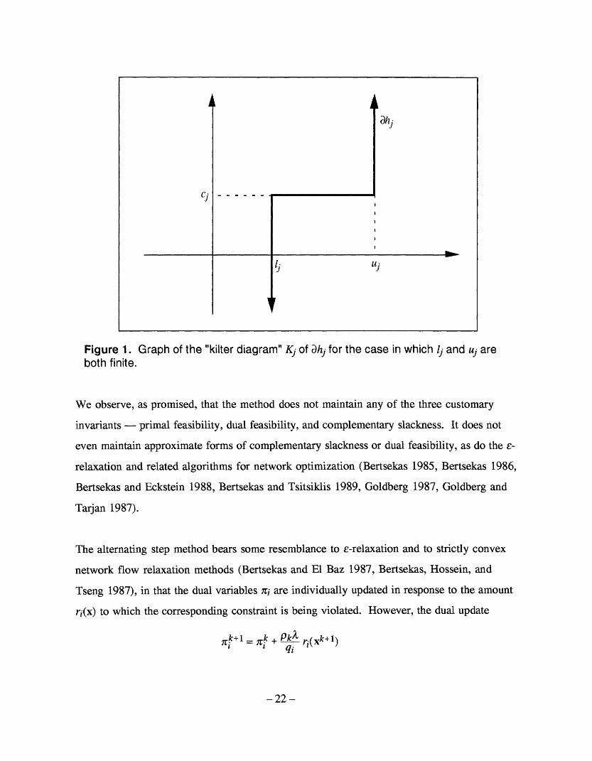
CI uh

Figure 1. Graph of the "kilter diagram" Kj of ahj for the case in which Ij and uj areboth finite.

We observe, as promised, that the method does not maintain any of the three customary

invariants - primal feasibility, dual feasibility, and complementary slackness. It does not

even maintain approximate forms of complementary slackness or dual feasibility, as do the E-

relaxation and related algorithms for network optimization (Bertsekas 1985, Bertsekas 1986,

Bertsekas and Eckstein 1988, Bertsekas and Tsitsiklis 1989, Goldberg 1987, Goldberg and

Tarjan 1987).

The alternating step method bears some resemblance to e-relaxation and to strictly convex

network flow relaxation methods (Bertsekas and El Baz 1987, Bertsekas, Hossein, and

Tseng 1987), in that the dual variables 7ri are individually updated in response to the amount

ri(x) to which the corresponding constraint is being violated. However, the dual update

i -sr i + RPkX r,(Xk+1)qj

-22-

is unique in that the dual adjustment is proportional to the surplus ri(xk+l), and the dual

variable may either rise or fall, depending on the sign of the surplus. In the e-relaxation and

related algorithms, dual variables can be adjusted in only one direction.

To further illuminate the comparison between the alternating step method and recent

proposed parallel methods for network optimization, consider the alternating step method

specialized to minimum cost network flow problems, with Pk fixed at 1. If one assumes that

A is the node-arc incidence matrix of a network and uses the index vw, rather than j, to

indicate arc (v, w), one obtains the method

X+1= PV(vw) kw+ I v ( xk) C vw(xk ) ) V arcs (v, w)K4 W2 2d(v) d(w) ;c

k +l= k+ d rv(xk+l) .V nodes vd(v)

Here, xvw denotes the flow on arc (v, w), ,v is the dual variable associated with node v, and

rv(x) is the amount of flow imbalance at node v. We offer the following interpretation: each

node v attempts to "push" away its surplus rv(xk), spreading it evenly among all its incident

arcs. If the surplus is negative, the node instead "pulls" flow evenly on all its incident arcs.

Each arc (v, w) then takes the two flows suggested by its "start" node v and "end" node w,

averages them, makes a further adjustment based on its reduced cost, and then projects the

result onto its feasible capacity range V(vw). Each node then makes a price adjustment

proportional to the surplus resulting from the new flows.

In summary, while there is some similarity to the alternating "pushing" and price adjustment

processes of e-relaxation, the rules governing these steps are quite different. Furthermore,

e-relaxation has not been generalized to constraint structures more complicated than

networks without gains, whereas the alternating step method may be applied to any

monotropic program.

-23 -

Another interesting feature of the alternating step method is that it does not solve a linear

system of equations at each iteration, nor does it update a solution to such a system, as does

the simplex method. However, by setting cj = O, Ij = -oo, and uj = + oo for all j, it could be

used to solve the system of equations Ax = b. Thus, it is an iterative method that appears to

be equally suited to optimizing linear programs or solving linear systems.

5. Linear Convergence Rate

We now show that, so long as Pk < 1 for all k, the alternating step method for linear

programming converges at a globally linear rate, in the sense that the distance of {xk} to the

set of optimal solutions and the distance of I{k} to the set of optimal simplex multipliers are

bounded above by convergent geometric sequences. Because of the complexity of the

analysis, this section assumes familiarity with the proximal point theory developed in

Eckstein and Bertsekas (1989).

We have already seen that the alternating step method is equivalent to the generalized

alternating direction method of multipliers under certain choices off, g, and M. From Eckstein

and Bertsekas (1989), we also know that this application of the generalized alternating

direction method of multipliers is equivalent to the generalized proximal point algorithm

tk+ l = (1 - Pk)tk + Pk(I + ckS)-l(tk) ,

where ck = 1 for all k > 0, and S is a certain set-valued maximal monotone operator. The key

to the analysis is that the sequence {tk} produced by this recursion converges to some zero

of S, that is, a point t* such that 0 E S(t*). The set of lJIJ .suwh .7.rs . tJ nePid S-l(0).

Figure 2 is intended to clarify the role of the relaxation factor Pk in the convergence of the

method. For p E (0, 2), let

tk+l(p) = (1 - p)tk + p(I + ckT)-l(tk)

From the figure, it is clear that

-24 -

for all p < 1 and t* E S- 1(0), so choosing p < 1 is unlikely to be beneficial. On the other hand,

there may be an interval (1, p) c_ (1, 2) on which p E (1, p-) implies

dist(tk+l(p), S-1(0)) < dist(tk+l(1), S- 1(0))

Thus, it should be possible for over-relaxation to accelerate convergence.

Possible range oftk+l(p)

tk+ 1(1) tk

... .. : ........v ...... ::::::::- .. ...... -:::-:::: :::-:. -... ::. : :

Figure 2. Illustration of the use of the relaxation parameters Pk. Here, tk+l(l) =(I + S)-l(tk), and t* is an arbitrary member of S-1(0). Because of the maximalmonotonicity of S, the angle 0 must be at least 90 degrees and the set S1(0) mustbe closed and convex.

Referring to Eckstein and Bertsekas (1989), and adopting that paper's notational convention

that S = { (t, w) I w e S(t)}, that is, that there is no distinction between an operator and its

graph, the expression for S is

S = {(v + Xb, u-v) i (u, b) e B,(v, a) E A, v+X.a = u - .b},

where A and B are the maximal monotone operators

-..25 -- 25 -

A = = -M()] = - f)-l (- M T)

B = g = (ag)- 1

on 1~nm. The equivalence of the two expressions for A is guaranteed because the column

space of -M r is all of 1n (Rockafellar 1970, Theorem 23.9). The basic approach to obtaining

a linear convergence rate is based on that of Luque (1984), and hinges on the following

question: is there a constant a such that w E S(t) implies dist(t, S-1(0)) < all w II ? To

answer this question, we must examine the structure of the operators A, B, and S.

First,

af c+x E X < u j 0, j> =j 0 , I < x < u

)f(x) ~0' otherwise .

Thus,

(af)-l(y)= { xE n I I < x< U, yjcjc xj=lj, yj > c xj=uj},

and so for any q E IR.m n ,

Aq = -M(af)-l(-MTq)

= {[-aijxj] e Rmn xe Rn,I <x<u, xj= Ij Vj: Cj+ m=L1 aijqij > 0,

xj=yuj j: cj + m= 1 aijqij < 0 }.

As for B = (0g)-1, we have

g(q) L0, q C

where VL is the orthogonal complement of the linear subspace V parallel to C, namely

VL = { pE Rlmn I Pij =Pil V (i,j), (i, ) Q} .

It then follows that for any p E V-, Bp = C, and otherwise Bp=0.

-26 -

We will now draw a connection with linear programming stability theory. We define x E I n

to be 3balanced if 1 < x < u and Ilr(x)100 < 5, that is, if ri(xk) < 3 for i = l,...,m. We also say

that (x, G) E 1Rn X Em obey e-complementary slackness (Tseng and Bertsekas 1987) if

I < x < u and

xj > lj = cj(1) < E

xj < Uj cj() > - E .

Alternatively, x is 3-balanced if and only if it is feasible for some problem obtained from (LP)

by replacing b by some b', where 11 b -b' II. < 6, and (x, n) obey e-complementary slackness

if and only if they obey conventional complementary slackness with respect to some costs c',

where 11 c - c' lloo < e.

Choose the sets Qi as in the proof of Theorem 2. We now state a technical lemma:

Lemma 5. Suppose (t, w) E S. Then there exist p, q, s, z E Rmn, x E ER!n, and X E Rm such

that

(p, z) E B(q, s) E Aq+Xs = p - Xzq+Lz=tp-q=wsij = - aijxj for i = l,...,m,j=l,...,nXi = - Pij for all (i, J) e Q,

and for any p, q, s, z, x and X satisfying these conditions,

x is dmaxllWll/X-balanced

(x, g) obeys amaxllwll-complementary slackness,

A where amax = max j=l,...,n {1la 1ll} and d max i

Proof. From the definition of S,

S = {(q + Xz, p - q) (p, z) B, (q, s) E A, q+s = p - Xz},

-27 -

we immediately have the existence of p, q, s, z E Rmn satisfying the first five conditions,

(p, z) E B(q, s) e Aq+Ls = p- Zzq+zz =tp-q=w.

In accordance with (q, s) E A and the form of A, let x' E Rn be such that x' obeys the bounds 1

• x' < u, xj' = Ij for all j such that cj + Jm= 1 aijqij > O, xj = uj for allj such that c+ m=

aijqij < 0, and sij = - aijxj' for all i and j. Given any x with the property

sij = - aijxj for all i and j, the fact that A has no zero columns gives x' = x. Note that q +Ls =

p - Lz implies a(s + z) = p - q = w. We have

[s + z]ij = zij- aijxj V i, j,

and, as 1Is + zl[ = Ilwll/X,

zij y-aijxjl < Ilwll/L V i, j,

whence

I E (zij- aijxj) I < d(i)Jlw}/X V i.

j: aO' o

Since (p, z) E B = V 1 x C, we must have z E C, and so zj= bi for all i. Thus, the last

inequality is equivalent to

I bi - AiTX I = Iri(x) I < d(i)llwll/X V i.

Thus, using the definition of dmax, we conclude that the primal solution x is dmaxIlwll/X-

balanced.

From (p, z) E B = V-Lx C, we also have p E V- , hence Pij = Pil for all (i, j), (i, I) E Q. In

particular, pij = pil for all (i, j), (i, 1) such that aij, ail * O. Then it is possible to uniquely

define c E JRm via iri' = - Pij for all (i, j) such that aij : O. We now consider p and q. For all j,

-28 -

I =l 1aij(pijl- qij)= I a T( + qj ) I < Iaj1- 11 + qj

where qj is the m-vector consisting of the {qij} i 1. Since 11 p - q 11 = liwll, II c + qj 11 < liwll,

and thus

I m 1 aij(Pij - qij) I <- la/ 11Llwil

Using that (q, s) E A, we have

xj c + m aijqij > 0 (cj- aij(Pi j - qij)) -= 1 aijni > O

xj > Ij = cj + ]m= 1 aijqij < O (cj - £m= aij(pij- qij)) - _ I aijii < o

Thus, (x, a;) obey complementary slackness if we permit a perturbation of each cost

coefficient cj by an amount m= 1aij(Pij - qij), whose magnitude cannot exceed Ilajl Ilwll.

Using that amax = max j {llall }, we conclude (x, wi) obeys amaxllwll-complementary slackness.

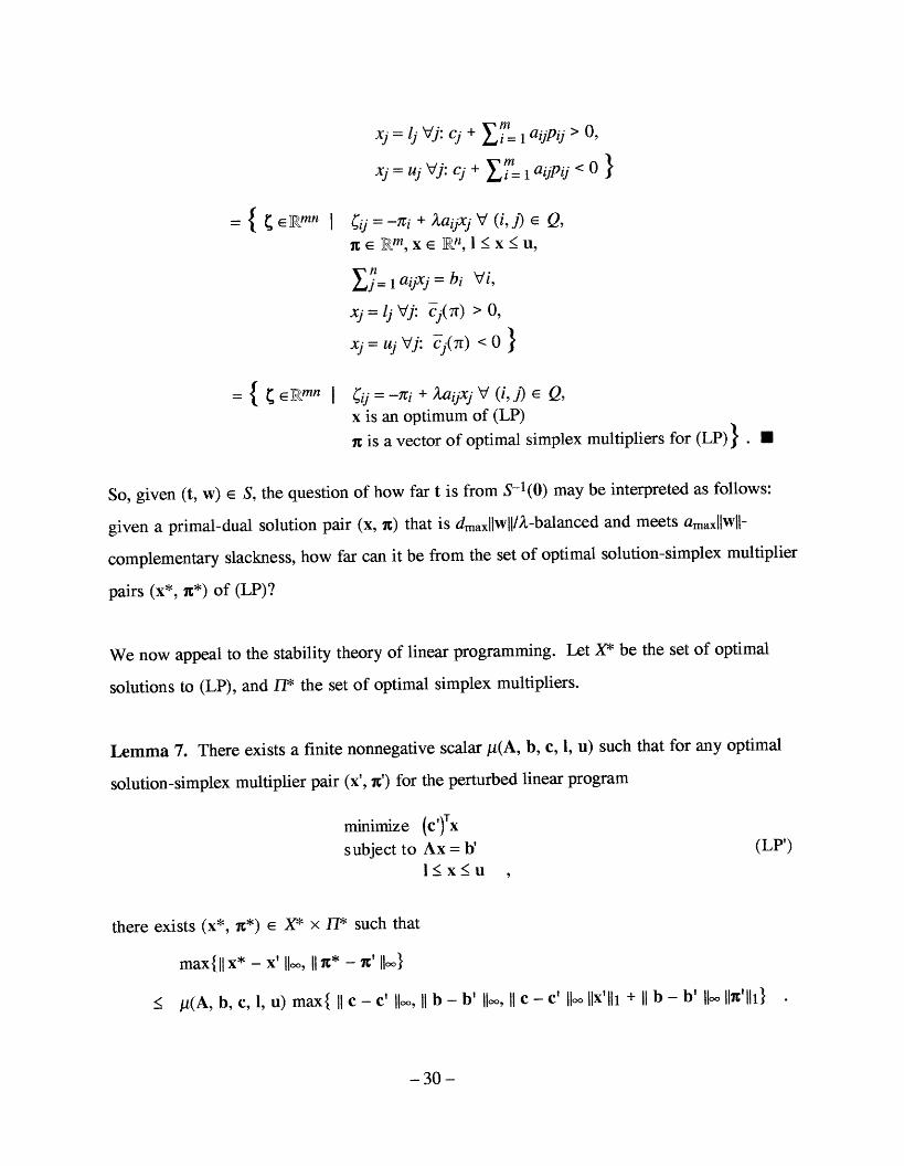
We now precisely characterize the zeroes of the operator S.

Lemma 6. For the choices of the maximal monotone operators A and B used in the

alternating step method for linear programming,

S-l(0) = { R mn I ~ij = -7i + Xaijxj V (i,) E Q,x is an optimum of (LP)

i is a vector of optimal simplex multipliers for (LP) .

Proof. Using Theorem 5 of Eckstein and Bertsekas (1989) and the form of A and B,

S-l(O) = {p+Zz I (p, z) E B, (p, -z) E A}

= { [Pij +,aijxj] I Pij = pil (i, j), (i, 1) e Q,x E 1Rn, 1 < x < u,

Ej= 1 aiixj = bi Vi,

-29 -

x IjVj: c + .i= aijpij > 0,

Xj = uy Vi: cj + i = aijPij c< }

={ { eRmn I 5ij =-rCi + aijxj V (i,j E Q,

K E j m, x E En, I < x < U,

j aixj j= bi Vi,

xj = Ij Vj: Cj(Tr) > O,

xj= uj Vj: C(~) < }

{ ;,mn [I j = -ri '+aij=axj V (i, j) E Q,

x is an optimum of (LP)

c is a vector of optimal simplex multipliers for (LP) } .

So, given (t, w) E S, the question of how far t is from S-1(O) may be interpreted as follows:

given a primal-dual solution pair (x, K) that is dmaxllwll/X-balanced and meets amallwll-

complementary slackness, how far can it be from the set of optimal solution-simplex multiplier

pairs (x*, n*) of (LP)?

We now appeal to the stability theory of linear programming. Let X* be the set of optimal

solutions to (LP), and H* the set of optimal simplex multipliers.

Lemma 7. There exists a finite nonnegative scalar p(A, b, c, 1, u) such that for any optimal

solution-simplex multiplier pair (x', K') for the perturbed linear program

minimize (c')Tx

subject to Ax = b' (LP')l<x<u

there exists (x*, K*) E X* x 1* such that

max{11 x* - x' Iloo, 1I X* - e' lloo}

< ,u(A, b, c, 1, u) max{ II c - c' Iloo, Ii b - b' Iloo, II c - c' IIoo II'IIl1 + II b - b' hloo I!'11l}

-30 -

Proof. We give a proof for the case that (LP) is in the standard primal form where Ij = 0 and

Xj = +oo for all j. The proof for other cases is entirely analogous. If (LP) has this form, then

(x, 1) is an optimal pair if and only if it solves the linear system

Ax = b- Ix <0 (*)

AT;i < C

cTx - bTn <0 ,

whereas we have

Ax' = b'- Ix' <0

ATWt' < C'c'Tx' - b'TI-' < 0

We may rewrite this last inequality as

CTX' - bT;' < (C - C')TX' - (b - b')T' ,

we conclude that (x', ;') is one possible solution in (x, n) of the system

Ax = b'- Ix <O

ATx < c'

CTX - bTi < (c - ')Tx ' - (b - b')T' ,

which differs from (*) only in the right-hand side. Then from Mangasarian and Shiau (1987),

Theorem 2.2, there exists a finite scalar > 2> 0 such that for all choices of b' and c',

b'-b

(x',~')-(x*.~*)~l <-' t c'-c

(C-c'-)Tx' + (b- b')T 'Tn'

< , max {b'- b .1, i c'- l (c -c')Tx'+ (b-b')T

< g max { b'-bIloo, II c'-c looII c'-c !IOlix'lil + II b'-bIIlool1iI }

Let tk= pk + Azk for all k > 0. Then, from Eckstein and Bertsekas (1989),

-31-

tk+l = (1 - pk)t k + pk(l + S)-I(tk)

= [I- pk(I - (I + S)-l)](tk)

= (I- pkK)(tk)

where K is the operator I - (I + S)- 1.

Lemma 8. Let 0 = inf {pk(2 - Pk) I k > 0} E (0, 1]. Then the following inequalities hold for

all k2 0:

(i) lltk+l - t* 112 < lItk - t* 112 - 011K(tk) 112 for all t* E S-1(0)

(ii) dist2 (tk+l, S-1(0)) < dist2(tk, S- 1(0)) - 011 K(tk)l112

Proof. From the proof of Theorem 3 of Eckstein and Bertsekas (1989), we have for all k 2 0

and t* E S-1(0) that

I tk+l - t* 112 < Itk - t* 112 - pk(2 - pk) II K(tk) 112

which implies (i). One then obtains (ii) by taking t* in (i) to be the projection of tk onto

S-1(0) (which is closed and convex by the maximality of S). ·

We know from Theorem 3 that if (LP) is feasible and bounded, that {xk} and { ik} are

bounded sequences. Define

D x = sup (llxkl11) < o

= sup ll < k>O

Rx = max {1, Dx}

RC = max { 1, Do}

y = /,(A, b, c, 1, u) [amaxRx + - -R r]

-32 -

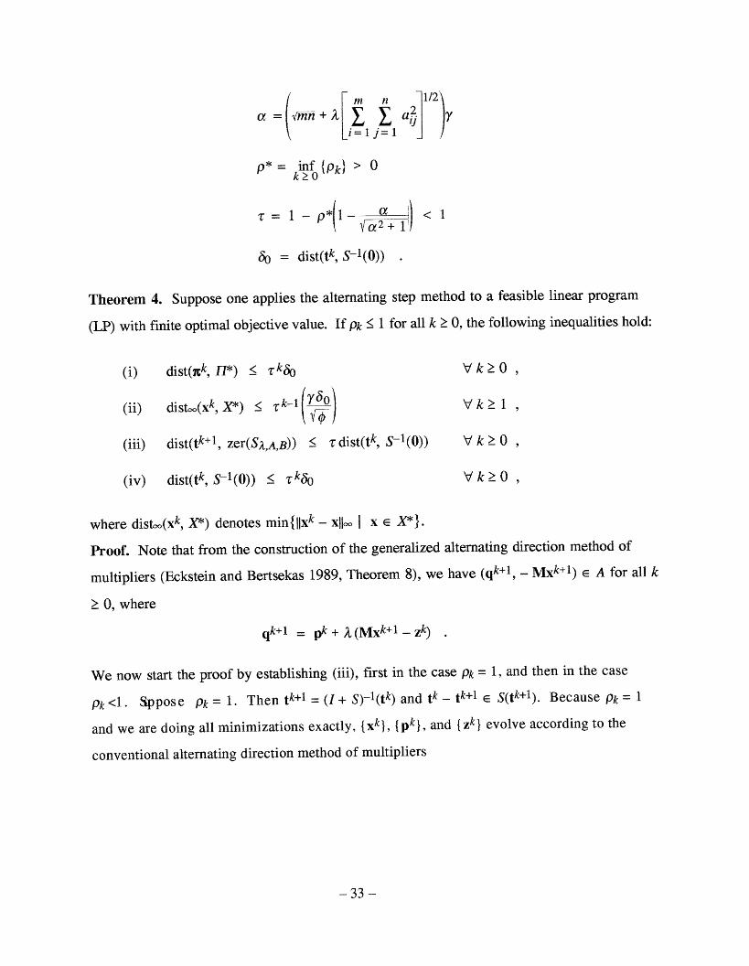
a Vm-n + a+ L

P*= inf {Pk) > 0

P= 1-p*l /- < 1

0 = dist(tk, S-l(0))

Theorem 4. Suppose one applies the alternating step method to a feasible linear program

(LP) with finite optimal objective value. If Pk < 1 for all k > 0, the following inequalities hold:

(i) dist(nk, H*) < k30 V k 0 ,

(ii) dist(Xk, X*) < r k - l (6 5 ) Vk> 1

(iii) dist(tk+l, zer(Sx,,A,B)) < zdist(tk, S-l(O)) Vk20 ,

(iv) dist(tk, S1 (0)) < zko V k > 0,

where distoo(xk, X*) denotes min{llxk - xllo I x E X*}.

Proof. Note that from the construction of the generalized alternating direction method of

multipliers (Eckstein and Bertsekas 1989, Theorem 8), we have (qk+l, - Mxk+l) E A for all k

> 0, where

qk+l = pk + Z (Mxk+l - zk)

We now start the proof by establishing (iii), first in the case Pk = 1, and then in the case

Pk <1. Sppose Pk = 1. Then tk+l = (I + S)-l(tk) and tk - tk+l e S(tk+l). Because Pk = 1

and we are doing all minimizations exactly, {xk}, {pk}, and {zk} evolve according to the

conventional alternating direction method of multipliers

-33 -

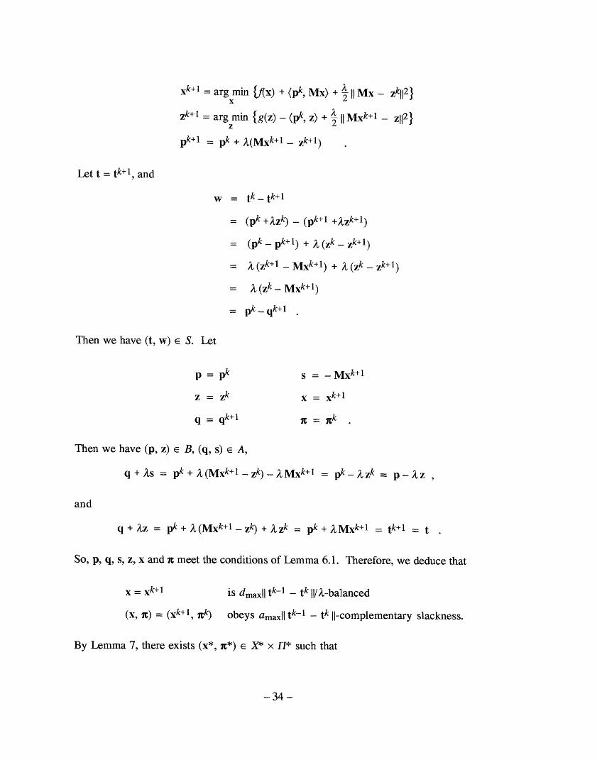
xk+1 - arg min {flx) + (pk, Mx) + 2 11 Mx - zkil2 }X 2

zk+l = arg min {g(z) - (pk, z) + A 11 Mxk+1 - z112}

pk+l = pk + X(Mxk+l - zk+l)

Let t = tk + l, and

w = tk tk+ l

= (pk + Xzk) - (pk+ +Azk+ 1

= (pk_ - pk+l) + X (zk _ zk+l)

= X (z k + l - Mxk+ l ) + 2, (zk _ zk+l )

= , (zk - Mxk+1)

pk_ qk+l

Then we have (t, w) E S. Let

p = pk s = -sMxk + l

z = zk x = x k +l

q = qk+l 1 = kk

Then we have (p, z) E B, (q, s) E A,

q + Xs = pk + (Mxk+l _z k ) _ Mxk+ l = pk_ Xzk = p-_z ,

and

q + z = pk + X(Mxk+l - zk) + zk = pk + XMxk+l = tk+l = t

So, p, q, s, z, x and 1i meet the conditions of Lemma 6.1. Therefore, we deduce that

x = xk+l is dmaxll tk-l - tk 11/X-balanced

(x, g) = (xk+ l, nk) obeys amaxll tk-l - tk II-complementary slackness.

By Lemma 7, there exists (x*, c*) E X* x H* such that

-34 -

.ma.rt Il - ' 'l IIl" '

- ' 1" J1

< ,u(A, b, c, I, u) max{ amaxll t k - l - tk 11,dmaxli tk- l - tk I/X,amaxll tk-l - tk 11 IIx'lII + dmaxl tk-l - tk II IlI11;ll/X}

< j(A, b, c, 1, u) [amaxRx + jdRir] IItk -l _ tk I1

y 1 tk-l1 - tk II

Defining p* by

P* = i* ' (i,j) e QPij_ 0, (i, j) Q

we have that t* = p* + XMx* E S-1 (0). Also,

IItk+l - t*1t < 1lpk - P*11 + IIMxk+l- Mx*11

< lipk - p*11 + XIIM(xk+l - x*)11

m n 1/2

< mip -p*k-Pll + j1 aj iIxk+l - x*1OOi=l j=l

, mmn llN k- -r*11 + A 1 aI IIxk+l - x*11oi= lj=l

m n 1/2< mnTy Iltk _ tk+lll + A ]£ 1 a ?j Iltk - tk+ll1

i=l j=l

=a IItk - tk+lll .

Thus,

dist(tk+l, S-1 (0)) < a Iltk- tk+111

When Pk = 1, the inequality

-35 -

II tk+l- t* 112 < II tk - t* 112 _ pk(2 - pk) II Q(tk) 112 V t* e S-1 (0)

reduces to

I tk+l -_ * 112 < 11 tk- t* 112 - litk - tk+1112 V t* E S-1(0),

implying

dist2(tk+l, S- 1(0)) < dist2(tk, S- 1(o)) - Iltk - tk+lll2

Hence,

dist2(tk+l, S-1 (0)) < dist2(tk, S-1(0)) - 12 dist2(tk+1, S-1())

Simplifying and taking the square root, we obtain

dist(tk+l, S-l(0)) < a dist(tk, S-1(0)) < rdist(tk S-l(0))

This gives (iii) in the case that Pk = 1. Now consider the case Pk < 1. Let

uk+l = (I + S)-l(tk

be the value that tk+1 would have taken had Pk been 1. Then we have

tk+l = (1 - Pk)tk + pkuk+l

and, by the convexity of the function dist( -, S1 (0)), we have

dist(tk+ l, S-1 (0)) < (1 - pk)dist(tk, S-1(0)) + pkdist(uk+l, S-1(0))

< (1-p- Pk(1- 2a ) dist(tk, S-1 (0))

< Tdist(tk, s-l(0))

which gives (iii). By induction, we obtain (iv).

-36 -

We now demonstrate (i) and (ii). For all k 2> 0, there exists some t*k E S-l(0) such that

IItk - t*kll •< rk60. Applying the nonexpansive operator (I + XB)- l to tk and t*k, one obtains

IIpk - p*kII < ko60, where p*k and z*k are such that

t*k = p*k + Xz*k

(p*k, z*k) E B

(p*k, _ z*k) e A

It follows that II k- K_*k;l < TkM, where I*k CE H* is defined by iri*k = -pij*k for all (i,J) E Q.

This fact implies (i). Finally, for k >0, we have from above that there exists x*(k+l) such that

I xk+l x*(k+l)loo < y l tk - Uk+l = Y K(tk)II

By Lemma 8,

II K(t" 112 < 1 dist2 (tk, S-l(0))

hence

1xk+1 - x*(k+l) 11oo < (-3)

which gives (ii). ·

A few comments: it is possible to place explicit bounds on the quantities /.t(A, b, c, 1, u), Dx,

and Dx, and hence on the other constants used in the proof. This analysis was omitted in the

interest of brevity, but can be found, in the case that all entries of A are integer, in Eckstein

(1989). The question of linear convergence in the case that Pk > 1 for an indefinite number of

k remains open. The general convergence methodology of Luque (1984) does not seem to

extend easily to the proximal point algorithm with over-relaxation (Pk > 1), although it does

apply to under-relaxation (Pk < 1).

-37 -

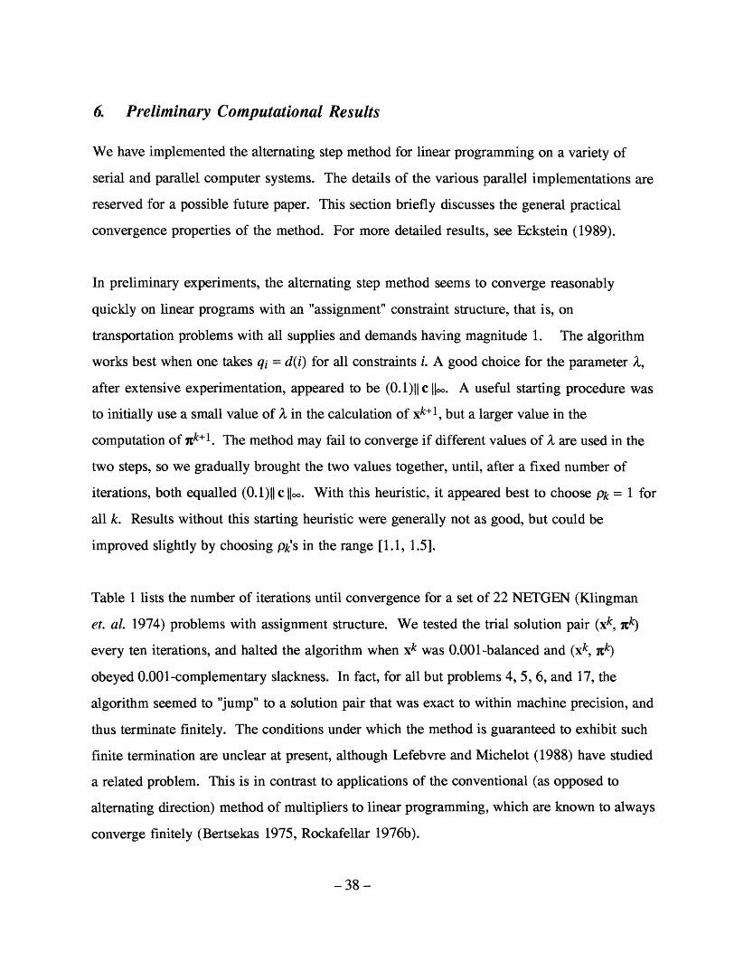
6. Preliminary Computational Results

We have implemented the alternating step method for linear programming on a variety of

serial and parallel computer systems. The details of the various parallel implementations are

reserved for a possible future paper. This section briefly discusses the general practical

convergence properties of the method. For more detailed results, see Eckstein (1989).

In preliminary experiments, the alternating step method seems to converge reasonably

quickly on linear programs with an "assignment" constraint structure, that is, on

transportation problems with all supplies and demands having magnitude 1. The algorithm

works best when one takes qi = d(i) for all constraints i. A good choice for the parameter X,

after extensive experimentation, appeared to be (0.1)1I c IIo. A useful starting procedure was

to initially use a small value of X in the calculation of xk+l, but a larger value in the

computation of xk+l. The method may fail to converge if different values of .X are used in the

two steps, so we gradually brought the two values together, until, after a fixed number of

iterations, both equalled (0.1)11 c IIoo. With this heuristic, it appeared best to choose Pk = 1 for

all k. Results without this starting heuristic were generally not as good, but could be

improved slightly by choosing pk's in the range [1.1, 1.5].

Table 1 lists the number of iterations until convergence for a set of 22 NETGEN (Klingman

et. al. 1974) problems with assignment structure. We tested the trial solution pair (xk, ck)

every ten iterations, and halted the algorithm when xk was 0.001-balanced and (xk, sk)

obeyed 0.001-complementary slackness. In fact, for all but problems 4, 5, 6, and 17, the

algorithm seemed to "jump" to a solution pair that was exact to within machine precision, and

thus terminate finitely. The conditions under which the method is guaranteed to exhibit such

finite termination are unclear at present, although Lefebvre and Michelot (1988) have studied

a related problem. This is in contrast to applications of the conventional (as opposed to

alternating direction) method of multipliers to linear programming, which are known to always

converge finitely (Bertsekas 1975, Rockafellar 1976b).

-38 -

Sourcesi CPUProblem Sinks Arcs II c llI Iterations Seconds

1 4 16 982 60 0.02

2 32 100 100 60 0.03

3 32 400 100 110 0.13

4 32 600 100 1020 1.47

5 32 800 100 770 1.40

6 32 900 100 350 0.70

7 32 1024 100 60 0.15

8 32 1024 100 50 0.12

9 32 1024 100 60 0.13

10 1024 5120 100 440 7.13

11 1024 5120 100 770 12.57

12 1024 5120 100 930 15.52

13 1024 5120 100 800 13.23

14 200 1000 100 180 0.58

15 400 2000 100 390 2.48

16 600 3000 100 430 4.07

17 100 500 100 490 0.83

18 105 525 200 140 0.25

19 110 550 400 160 0.32

20 115 575 800 140 0.27

21 129 600 1600 140 0.28

22 125 625 3200 150 0.32

Table 1. Detailed results for a FORTRAN implementation of the alternating stepmethod on linear programs with "assigment" constraint structure. CPU times arefor an Alliant FX/8, a "supermini" computer allowing a modest degree ofparallelism.

-39-

The results of Table 1 are fairly encouraging. With large speedups due to its inherent

parallelism, the alternating step method should prove quite competitive for problems of this

type.

For more general linear programs, including transportation problems, our early computational

experiments have been much less encouraging; the method seems prone to a curious "spiral"

convergene behavious, which we now illustrate. For all k 2 0, let

imax(k) = arg max ,{ I ri(xk) |i=l1,...,m

rmax(k ) = r[ix(k)l(xk)

Cj(7ck), tj CJ xk < ui

sj(k) = imax {cj(Ik) 0}, xJ = uk j = 1,...,n

min {-Cj(k), O}, xk = I

imax(k) = arg max { sj(k) | }

a(k) = S [jix(k)](k)

so that I rmax(k) I is an estimate of the feasibility of xk and I o(k) I is an estimate of how

closely (xk, uk)complementary slackness.

For a small transportation problem, Figure 3 shows a typical plot of rmax(k) and ac(k) for

large k; the graphs forms a very slowly-converging spiral around (0, 0). At present, we are

not sure how to accelerate this convergence behaviour.

So far, we have not tested the alternating step method on nonlinear monotropic programs. It

will be interesting, for instance, to compare it to dual relaxation methods for nonlinear

network problems (Bertsekas and E1l Baz 1987, Bertsekas, Hossein, and Tseng 1987, Zenios

and Lasken 1988). Unlike such dual relaxation methods, the alternating step method can

-40 -

solve problems with mixtures of linear cost and strictly convex cost arcs, and can handle

constraint structures more general than pure networks.

0.10

0.00

, -0.05

-0.10 - . , . , . , . . . . . .I-0.10-0.20 -0.15 -0.10 -0.05 0.00 0.05 0.10 0.15 0.20

Largest-Magnitude Complementary Slackness Violation

Figure 3: Data from a run of the alternating step method on a smalltransportation problem, depicting the largest-magnitude surplus rmx(k)versus the largest-magnitude complementary slackness violation a(k) forlarge k.

References

BERTSEKAS, D. P. (1975), "Necessary and Sufficient Conditions for a Penalty Method to beExact". Mathematical Programming 9:87-99.

BERTSEKAS, D. P. (1982), Constrained Optimization and Lagrange Multiplier Methods (NewYork: Academic Press).

BERTSEKAS, D. P. (1985), A Distributed Asynchronous Relaxation Algorithm for theAssignment Problem. Proceedings of the 24th IEEE Conference on Decision and Control,Fort Lauderdale, Florida, 1703-1704.

BERTSEKAS, D. P. (1986), Distributed Asynchronous Relaxation Methods for Linear NetworkFlow Problems. Report LIDS-P-1606, Laboratory for Information and DecisionSciences, MIT. (Original Report, September 1986, revised version, November 1986.)

-41 -

BERTSEKAS, D. P., ECKSTEIN, J. (1988), "Dual Coordinate Step Methods for Linear NetworkFlow Problems". Mathematical Programming 42(2):203-243.

BERTSEKAS, D. P., EL BAZ, D. (1987), "Distributed Asynchronous Methods for ConvexNetwork Flow Problems". SIAM Journal on Control and Optimization 25(1):74-85.

BERTSEKAS, D. P., HOSSEIN, P., TSENG, P. (1987), "Relaxation methods for network flowproblems with convex arc costs". SIAM Journal on Control and Optimization 25:1219-1243.

BERTSEKAS, D. P., TSITSIKLIS, J. (1989), Parallel and Distributed Computation: NumericalMethods (Englewood Cliffs: Prentice-Hall).

DE LEONE, R., MANGASARIAN, O. L. (1988), "Serial and Parallel Solution of Large ScaleLinear Programs by Augmented Lagrangian Successive Overrelaxation". InOptimization, Parallel Processing, and Applications, A. KURZHANSKI, K. NEUMANN,and D. PALLASCHKE, editors, Lecture Notes in Economics and Mathamatical Systems304 (Berlin: Springer-Verlag).

ECKSTEIN, J. (1988), The Lions-Mercier Algorithm and the Alternating Direction Method areInstances of the Proximal Point Algorithm. Report LIDS-P-1769, Laboratory forInformation and Decision Sciences, MIT.

ECKSTEIN, J. (1989), Splitting Methods for Monotone Operators with Applications to ParallelOptimization. Doctoral dissertation, department of civil engineering, MassachusettsInstitute of Technology. Available as report LIDS-TH-1877, Laboratory for Informationand Decision Sciences, MIT, or report CICS-TH-140, Brown/Harvard/MIT Center forIntelligent Control.

ECKSTEIN, J., BERTSEKAS, D. P. (1989). On the Douglas-Rachford Splitting Method and theProximal Point Algorithm for Maximal Monotone Operators. Report CICS-P-167,Brown/Harvard/MIT Center for Intelligent Control Systems, or Harvard BusinessSchool working paper 90-033 (Revision conditionally accepted to MathematicalProgramming).

FoRTIN, M., GLOWINSKI, R. (1983), "On Decomposition-Coordination Methods Using anAugmented Lagrangian". In M. FORTIN, R. GLOWINSKI, editors, AugmentedLagrangian Methods: Applications to the Solution of Boundary-Value Problems(Amsterdam: North-Holland).

GABAY, D. (1983), "Applications of the Method of Multipliers to Variational Inequalities".In M. FORTIN, R. GLOWINSK1, editors, Augmented Lagrangian Methods: Applicationsto the Solution of Boundary-Value Problems (Amsterdam: North-Holland).

GABAY, D., MERCIER B. (1976), "A Dual Algorithm for the Solution of Nonlinear VariationalProblems via Finite Element Approximations". Computers and Mathematics withApplications 2:17-40.

-42 -

GLOWINSKI, R., LE TALLEC, P. (1987), Augmented Lagrangian Methods for the Solution ofVariational Problems. MRC Technical Summary Report #2965, Mathematics ResearchCenter, University of Wisconsin - Madison.

GLOWINSKI, R., LIONS, J.-L., TREMOLIERES, R. (1981), Numerical Analysis of VariationalInequalities (Amsterdam: North-Holland).

GLOWINSKI, R., MARROCO, A. (1975), "Sur L'Approximation, par Elements Finis d'Ordre Un,et la Resolution, par Penalisation-Dualit6, d'une Classe de Problemes de Dirichlet nonLineares". Revue Francaise d'Automatique, Informatique et Recherche Opfrationelle9(R-2):41-76 (in French).

GOLDBERG, A. V. (1987), Efficient Graph Algorithms for Sequential and Parallel Computers.Technical Report TR-374, Laboratory for Computer Science, MIT.

GOLDBERG, A. V., TARJAN, R. E. (1987), Solving Minimum Cost Flow Problems bySuccessive Approximation, Proceedings of the 19th ACM Symposium on the Theory ofComputation.

GOL'SHTEIN, E. G. (1985), "Decomposition Methods for Linear and Convex ProgrammingProblems". Matekon 22(4):75-101.

GOL'SHTEIN, E. G. (1986), "The Block Method of Convex Programming". SovietMathematics Doklady 33(3):584-587.

KLINGMAN, D., NAPIER, A., STUTZ, J., (1974), "NETGEN - A Program for GeneratingLarge-Scale (Un)capacitated Assignment, Transportation, and Minimum Cost NetworkProblems". Management Science 20:814-822.

LEFEBVRE O., MICHELOT, C. (1988), "About the Finite Convergence of the Proximal PointAlgorithm". Trends in Mathematical Optimization: 4th French-German Conference onOptimization, International Series of Numerical Mathematics 84, K.-H. HOFFMANN ET.AL., editors (Basel: Birkhiuser-Verlag).

LIONS, P.-L., MERCIER, B. (1979), "Splitting Algorithms for the Sum of Two NonlinearOperators". SIAM Journal on Numerical Analysis 16(6):964-979.

LUQUE, F. J. (1984), "Asymptotic Convergence Analysis of the Proximal Point Algorithm".SIAM Journal on Control and Optimization 22(2):277-293.

MANGASARIAN, O. L., SHIAU T.-H. (1987), "Lipschitz Continuity of Solutions of LinearInequalities, Programs and Complementarity Problems". SIAM Journal on Control andOptimization 25(3):583-595.

ROCKAFELLAR, R. T. (1970), Convex Analysis (Princeton: Princeton University Press).

ROCKAFELLAR, R. T. (1976A), "Monotone Operators and the Proximal Point Algorithm".SIAM Journal on Control and Optimization 14(5):877-898.

-43 -

ROCKAFELLAR, R. T. (1976B), "Augmented Lagrangians and Applications of the ProximalPoint Algorithm in Convex Programming". Mathematics of Operations Research1(2):97-116.

ROCKAFELLAR, R. T. (1984), Network Flows and Monotropic Optimization (New York: JohnWiley).

SPINGARN, J. E. (1985A), "A Primal-Dual Projection Method for Solving Systems of LinearInequalities". Linear Algebra and Its Applications 65:45-62.

SPINGARN, J. E. (1985B), "Application of the Method of Partial Inverses to ConvexProgramming: Decomposition". Mathematical Programming 32:199-233.

SPINGARN, J. E. (1987), "A Projection Method for Least-Squares Solutions to Overdeter-mined Systems of Linear Inequalities". Linear Algebra and Its Applications 86:211-236.

TSENG, P., BERTSEKAS, D. P. (1987), "Relaxation Methods for Linear Programs".Mathematics of Operations Research 12(4):569-596.

ZENIOS, S. A., LASKEN, R. A. (1988), "Nonlinear Network Optimization on a MassivelyParallel Connection Machince". Annals of Operations Research 14:147-165

-44 -