an algorithm for computing solutions of variational ... · an algorithm for computing solutions of...

Numer. Math. (2010) 115:45–69DOI 10.1007/s00211-009-0270-2

NumerischeMathematik

An algorithm for computing solutions of variationalproblems with global convexity constraints

Ivar Ekeland · Santiago Moreno-Bromberg

Received: 12 April 2008 / Revised: 9 June 2009 / Published online: 15 October 2009© Springer-Verlag 2009

Abstract We present an algorithm to approximate the solutions to variationalproblems where set of admissible functions consists of convex functions. The mainmotivation behind the numerical method is to compute solutions to Adverse Selectionproblems within a Principal-Agent framework. Problems such as product lines design,optimal taxation, structured derivatives design, etc. can be studied through the scopeof these models. We develop a method to estimate their optimal pricing schedules.

Mathematics Subject Classification (2000) 49-04 · 49M25 · 49M37 · 65K10 ·91B30 · 91B32

1 Introduction

Isaac Newton was the first person to state and solve a variational problem with convex-ity constraints. In the Principia, he sought the shape of convex solid that encountersthe least resistance when moving through a fluid. The problem can be stated as follows.Let � be a smooth, convex subset of R

2. Define

We thank Guillaume Carlier and Yves Lucet for their thoughtful comments and suggestions. We wouldalso like to acknowledge two anonymous referees and the editor, whose thorough reading and suggestionsled to an improved version of our original manuscript.

I. EkelandDepartment of Mathematics, UBC, Canada Research Chair in Mathematical Economics,1984 Mathematics Road, Vancouver, BC V6T 1Z2, Canadae-mail: [email protected]

S. Moreno-Bromberg (B)Institut für Mathematik, Humboldt-Universität zu Berlin, Unter den Linden 6,10099 Berlin, Germanye-mail: [email protected]

123

46 I. Ekeland, S. Moreno-Bromberg

I [v] :=∫

�

dθ

1 + |∇v|2 , and C := {v : � → R | v is convex}.

One seeks the v in C which minimize(s) I . It should be noted that even if the Lagrangiansatisfied the necessary coercivity properties (see for example [11, Sect. 8]), the restric-tion v ∈ C would make it quite difficult to use the Euler–Lagrange equations, whichare satisfied only when the constraints are not binding. Newton solved the problem byassuming, quite naturally, that the function (and the domain) were radially symmetric.Four centuries later, Brock et al. [4] (see also [15]) showed that, if one removes the sym-metry assumption on the solution, one gets a lower minimum, and this result sparkednew interest to the study of variational problems with convexity constraints. At thesame time, such problems were also cropping up in finance and economics, because ofconcerns with asymmetry of information, particularly adverse selection (see [3] for acomprehensive account). Typically, when a monopolist addresses a market consistingof consumers with different tastes and means, he/she will not sell a single product,but will devise a line of products with different qualities and prices, each of whichaddresses a segment of the market. These products then compete with each other (evenif I am well off, I may want to buy the product devised for less wealthy people, eventhough the quality is less, because I find it a better bargain). The monopolist’s problem(also known in the economic literature as the principal-agent problem, the monopolistbeing the principal and the consumers the agents) is to devise a pricing schedule suchthat his/her profit is maximal. This is called non-linear pricing. The field took off in1978 with a seminal paper of Mussa and Rosen [17], and since then has produced aconsiderable stream of contributions ([2,7,19], etc.).

In models where goods are described by a single quality and the set of consumers isdifferentiated by a single parameter, it is in general possible to find closed form solu-tions for the pricing schedule, which is precisely the mathematical content of the paperby Mussa and Rosen. This is, however, not the case when multidimensional qualitiesand consumer types are considered. The question was first addressed by Rochet andChoné [19], who provided conditions for the existence of an optimal pricing rule andfully characterized the ways in which the monopolist discriminates among consumersin a multidimensional setting. They pointed out that it is only in very special casesthat one can expect to find closed form solutions. The same holds true for modelswhere the set of goods lies in an infinite-dimensional space, even when agent typesare one-dimensional. This framework was first used, to our knowledge, by Carlieret al. [7] to price OTC (over-the-counter) financial derivatives. It was then extendedby Horst and Moreno-Bromberg [12] to model the actions of a monopolist who hasan initial risky position that he/she evaluates via a coherent risk measure, and whointends to transfer part of his/her risk to a set of heterogenous agents. In both casesthe authors find that only very restrictive examples allow for explicit solutions.

Given that a great variety of problems, such as product lines design, optimal tax-ation, structured derivatives design, translate into variational problems with globalconvexity constraints, there is a clear need for robust and efficient numerical methodsthat approximate their solutions. Note here a particular requirement, which is an addi-tional burden on the numerics: the quantity of interest is not the solution itself, i.e. the

123

An algorithm for computing solutions of variational problems 47

maximizing function, but its gradient. Indeed, if f (x) is the solution, then ∇ f (x) isthe quality bought by consumers of type x .

The main difficulty is to find an approximation of the cone of convex functions.The first attempt in this direction, due to Kawohl and Schwab [13], consisted of usinga first-order finite elements method. Unfortunately it turned out to be flawed: indeed,Choné and Le Meur [9] proved that, given a family of structured meshes Mh , onecan always find a convex function u that is not a limit of convex functions uh , withuh piecewise linear on Mh . In other words, internal approximations with first-orderfinite elements are bound to fail, and the authors illustrate their point by numericalexamples. Carlier et al. [8] then introduced an external approximation by first-orderfinite elements, and showed that their algorithm converges when the functional to bemaximized (or minimized) is quadratic and there are no constraints. This is not the casefor the Rochet–Choné problem nor for most problems arising from economic theory,to which this method does not provide an answer. The editor has drawn our attentionto a very interesting paper by Anguilera and Morin [1], which appeared while this onewas being revised, and which takes yet another approach. Anguilera and Morin con-sider first- and second-order finite differences on a given family of structured meshesMh , which enables them do define a discrete gradient and a discrete Hessian; theythen consider the class of functions such that the discrete Hessian is non-negative, andprove that any convex function can be approximated in this way. On each mesh, thediscretized problem is solved using semi-definite programming (SDP), and when hgoes to 0 the corresponding solutions converge to the theoretical solution.

Our approach differs from the preceding ones. It is an interior method: at each stepthe approximate minimizer is convex. This is important from the economic point ofview because, as we mentioned earlier, the convexity condition embodies the infor-mation constraint which any proposed contract must satisfy: non-convex functionsrepresent contracts which cannot be implemented (i.e. agents will not behave in theway the principal expects). However, it is not a finite element method, nor does it usefinite differences or SPD: it relies on the well-known fact that a convex function is thesupremum of its affine minorants:

u(x) = sup(a,x∗)

{〈x, x∗〉 + a|∀y, 〈y.x∗〉 + a ≤ u(y)}

or, equivalently, of all its tangent hyperplanes:

u(x) = supy

{〈x − y, u′(y)〉 + u(y)}

We will replace the preceding formula by the following:

uh(x) = sup{〈x − y, u′(y)〉 + u(y)|y ∈ Mh

}

where Mh is a given mesh. It is clear that the function uh is convex, and we will showthat, under reasonable assumptions, it converges to u as the step h goes to 0. Thefunction uh is piecewise linear, in the sense that it is linear on certain cells downstairs,but these cells are unrelated to the mesh Mh we started from; in particular, they do

123


not have points in the mesh as vertices. In fact, the shape of these cells can be quitecomplicated, as illustrated in Figs. 5 and 6 of Sect. 4 (although, of course, they areconvex polyhedra). In this sense our method differs from a finite-elements method,where the given mesh determines the cells on which the approximate solution is linear(or rather, affine). This is why it evades the criticism of Choné and Le Meur: since thedecomposition into cells is not given a priori, but adapts to the solution, there cannotbe the same geometrical obstruction that befalls a decomposition where the shapesare defined a priori. The same reason may also explain why there are no geometri-cal obstruction either arising from the fact that our method uses simultaneously thefunction u and its gradient ∇u: since the decomposition into cells is unstructured, andadapts to the solution, it will also adapt to fit any integrability conditions. In Lachand-Robert and Oudet [14], have used a similar idea in a more geometrical setting: theyseek a convex body that minimizes a certain functional, and they proceed by startingfrom an admissible polyhedron and iteratively modifying the normals to the facets inorder to find an approximate minimizer.

We first apply our method to a benchmark problem, taken from Choné and Le Meur[9], where the solution can be computed explicitly, and we find that our method worksin situations where they find they do not have convergence. We then estimate the min-imizers for the well known Rochet–Choné problem (see [19]), where we find that oursolution matches the theoretical one, to a problem in OTC pricing of securities [7],and to a risk-minimization problem as in [12]. Our algorithm proves to be versatileenough to provide approximate solutions even when the criterion is non-convex, as in[7]. This is of particular interest for economic situations, since convexity goes hand-in-hand with the assumption that the agents have quasi-linear preferences, which inmany cases is simply too restrictive.

The remainder of this paper is organized as follows. In Sect. 2, we state our problemand provide our notation. Our algorithm and a proof of its convergence are presentedin Sect. 3, together with further discussion of the method. In Sect. 4, we show the solu-tions obtained via our algorithm to several problems found in the literature.1 Sincethese problems share a common microeconomic motivation, we include a brief dis-cussion on the latter. The examples include the well known Rochet–Choné problem, aone dimensional example from Carlier, Ekeland and Touzi and the risk transfer case ofHorst and Moreno-Bromberg for a principal who offers call options with type-depen-dent strikes and evaluates his/her risk via the “shortfall” of his/her position. This sectionis followed by our conclusions. Finally, the appendix is devoted to technical results.

2 Setting

Throughout this paper, we use the following notations:

• �, Q ⊂ Rn are convex and compact sets,

• µ denotes the Lebesgue Measure on Rn ,

• f is a (probability) density on �,• L(θ, z, p) = z − θ · p + C(p), where C is strictly convex and C1,

1 Our Matlab codes can be downloaded from: http://www2.hu-berlin.de/math-finance/?q=node/72.

123

http://www2.hu-berlin.de/math-finance/?q=node/72


• C := {v : � → R | v ≥ 0 is convex, and ∇v ∈ Q a.e},• I [v] := ∫

�L(θ, v(θ),∇v(θ)) f (θ)dθ .

Our objective is to (numerically) estimate the solution to

P := infv∈C

I [v]. (1)

Having in mind examples as the one presented in Sect. 4.1, we will refer to C asthe cost function. See Sect. 4.1 for the microeconomic motivation to the particularstructure of the Lagrangian. Given the properties of L and C we immediately have thefollowing

Proposition 2.1 Assume v solves P , then there is θ0 in � such that v(θ0) = 0.

Proof Let v0 = minθ∈� v(θ) (recall � is compact)and define u(θ) := v(θ) − v0,then

I [u] =∫

�

(u(θ) − θ · ∇u(θ) + C(∇u(θ))) f (θ)dθ = I [v] − v0 < I [v].

This would contradict the hypothesis of v being a minimizer of I over C unless v0 = 0.�

Remark 2.2 Notice that Proposition 2.1 would hold for any Lagrangian of the formL(θ, z, p) = G(θ, p) − θ · z for any strictly convex function G that does not dependon z.

It follows from Proposition 2.1 that we can redefine C to include only functionsthat have a root in �. This, together with the compactness of Q, implies the followingproposition, which we will use frequently.

Proposition 2.3 There exists 0 < K < ∞ such that v ≤ K for all v in C.

It follows from Proposition 2.3 and the restriction on the gradients that for eachchoice of cost function C , problem P has a unique solution, since the functional I willbe strictly convex, lower semicontinuous and the admissible set is closed and bounded(see [10]).

Remark 2.4 Our algorithm will still work with more general L’s as long as one canprove that the family of feasible minimizers is uniformly bounded.

3 The algorithm

This section contains a detailed description of our algorithm (Sect. 3.1), as well asa proof of its convergence (Sect. 3.2). From this point on, whenever we use super-scripts we refer to vectors. For example V k = (V k

1 , . . . , V km). On the other hand a

subscript indicates a function to be evaluated over some closed, convex subset of Rn

of non-empty interior, ie, {Vj } is a sequence of functions Vj : X → R for some Xcontained in R

n . We will only consider the domain � = [a, b]n . This choice is madefor computational simplicity and it plays no role in our proof of convergence.

123


3.1 Description

In order to find a interior approximation to the solution to P we proceed as follows:

1. We partition � into �k , which consists of kn equal cubes of volume µ(�k) :=( b−a

k )n . The elements of the partition �k will be denoted by σ kj , 1 ≤ j ≤ kn . Then

we define �k as the set of centers of the σ kj ’s. The elements of �k will be denoted

by θkj . The choice of a uniform partition is done for computational simplicity.

2. We denote f ki = ∫

σ ki

f (θ)dθ and associate such weight with θki .

3. We associate to each element θki of �k a non-negative number vk

i and an n-dimen-sional vector Dk

i . The former represents the value of v(θki ) and the latter ∇v(θk

i ).4. We solve the (non-linear) program

Pk := inf µ(�k)

kn∑i=1

L(θki , v

ki , Dk

i ) f ki (2)

over the set of all vectors of the form v = (v1, . . . , vkn ) and all matrices of theform D = (D1, . . . , Dkn ) such that:(a) v ≥ 0 (non-negativity),(b) Di ∈ Q for i = 1, . . . kn (feasibility),(c) vi − v j + Di · (θ j − θ i ) ≤ 0 for i, j ∈ {1, . . . , kn} i �= j (convexity).If the problem in hand includes Dirichlet boundary conditions these can be includedhere as linear constraints that the Dk

i ’s corresponding to points on the “boundary”of �k must satisfy.

5. Let (vk, Dk) be the solution to Pk . Define vk(θ) := maxi pi (θ), where

pi (θ) = vki + D

ki · (θ − θk

i ).

6. vk yields an approximation to the minimizer of P .

Remark 3.1 The constraints of the non-linear program determine a convex set. Noticethat the number of constraints associated to problem Pk over [a, b]n is kn + nkn +kn(kn − 1). The summands correspond to the positivity, feasibility and convexityconstraints respectively. Hence, this number grows polynomially with the number ofelements in the lattice and exponentially with dimension.

Remark 3.2 4 (c) guarantees that pi is a supporting hyperplane of the convex hull ofthe points {(θ1, v1), . . . , (θkn , vkn )}. Note that vk is a piecewise affine convex func-tion, but that the cells on which it is affine are unrelated to the cells of partition �k .We are not using a finite-elements method. This will be discussed further in Sect. 3,where examples will be given.

It should be noted that the evaluation of vk is non-local. This has the drawback ofbeing numerically very expensive; however, it yields intrinsically convex functions.Moreover, since these convex functions are lower semicontinuous (they are the point-wise supremum of linear functions) and finite, the algorithm produces continuousfunctions.

123


3.2 Convergence

In this section, we prove convergence of the algorithm. We denote, for notationalconvenience

Jk(vk, Dk) :=

kn∑i=1

(vk

i − θ i · Dki + C(Dk

i ))

µ(�k) f ki .

Proposition 3.3 Under the assumptions made on L, the problem Pk has a uniquesolution.

Proof The mapping

(vk, Dk) → Jk(vk, Dk)

is strictly convex. It follows from Proposition 2.3 that any feasible vector-matrix pair(vk, Dk) must lie in [0, K ]k ×Qk , which together with Remark 3.1 implies Pk consistsof minimizing a strictly convex function over a compact and convex set. The resultthen follows from general theory (see, for example [10]). � Proposition 3.4 There exists v ∈ C such that:

1. The sequence {vk} generated by the Pk’s has a subsequence {vk j }that convergesuniformly to v.

2. limk j →∞ I [vk j ] = I [v].Proof The bounded (Proposition 2.3) family {v j } is uniformly equicontinuous, as itconsists of convex functions with uniformly bounded subgradients (they are requiredto lie in Q). By the Arzela–Ascoli theorem we have that, passing to a subsequence ifnecessary, there is a non-negative and convex function v such that

vk → v uniformly on �.

By convexity ∇vk → ∇v almost everywhere (Lemma A.4); since ∇vk(θ) belongs tothe bounded set Q, the integrands are dominated. Therefore, by Lebesgue DominatedConvergence we have

limk→∞ I [vk] = I [v].

� Let u be the maximizer of I [·] within C. Our aim is to show that {vk} is a minimizing

sequence of problem P , in other words that

limk→∞ I [vk] = I [u] .

To this end, we need the following auxiliary definition:

123


Definition 3.5 Let u be such that infu∈C I [u] = I [u]. Given �k , define for i =1, . . . , kn :

1. uki := u(θk

i ),2. Gk

i := ∇u(θki ),

3. qi (θ) := uki + Gk

i · (θ − θki ), and

4. uk(θ) := maxi qi (θ).

Notice that uk(θ) is also constructed as the convex envelope of a family of affinefunctions. The inequalities

Jk(uk, Gk) ≥ Jk(v

k, Dk), (3)

and

I [vk] ≥ I [u] (4)

follow from the definitions of Jk(vk, D

k), vk and uk , as does the following

Proposition 3.6 Let u and uk be as above, then uk → u uniformly as k → ∞.

Proposition 3.7 For each k there exist ε1(k) and ε2(k) such that

∣∣∣Jk(vk, D

k) − I [vk]

∣∣∣ ≤ ε1(k), (5)

∣∣∣Jk(uk, Gk) − I [uk]

∣∣∣ ≤ ε2(k), (6)

and ε1(k), ε2(k) → 0 as k → ∞.

Proof We will show inequality (5) holds, the proof for (6) is analogous. Define thesimple function

wk(θ) := L(θkj , v

kj , D

kj ), θ ∈ σ k

j ,

hence

Jk(vk, D

k) =

∫

�

wk(θ)dθ. (7)

The left-hand side of (5) can be written as

∣∣∣∣∣∣∣∫

�

wk(θ)dθ − I [vk]

∣∣∣∣∣∣∣. (8)

123


It follows from Lemma A.6 that there exists ε1(k), such that

∣∣∣∣∣∣∣∫

�

wk(θ)dθ − I [vk]

∣∣∣∣∣∣∣≤ ε1(k),

and

ε1(k) → 0 when k → ∞.

� We can now prove our main theorem, namely

Theorem 3.8 The sequence {vk} is minimizing for problem P .

Proof It follows from Proposition 3.7 and Eq. (3) that

I [uk] + ε2(k) + ε1(k) ≥ I [vk] ≥ I [u]. (9)

Letting k → ∞ in (9) and using Proposition 3.4 yields the desired result. � Remark 3.9 In Choné and Le Meur [9] (see also Carlier et al. [8]), it was pointedout that, when using finite elements on regular meshes, one encounters a geometricalobstruction. Namely, let Tn be a sequence of quasiuniform regular triangulations Tn ,and suppose there are two vectors h and k such that, for every unit vector ν which isnormal to an edge of each element in the triangulation

〈ν, h〉 · 〈ν, k〉 ≥ 0.

Then, if u is the limit in L∞loc of a sequence of convex functions un which are piecewise

linear on the triangulation, we must have:

∂2u

∂h∂k≥ 0.

As Figs. 2 and 3 in the next section will show, the partition generated by our method isnot a triangulation, nor is it regular, so it is not affected by this geometrical obstruction.

4 Examples

In this section, we show some results of implementing our algorithm. The first threeexamples reduce quadratic programs, whereas the fourth and fifth ones are non-linearoptimization programs. All the computer coding has been written in Matlab. However,the supplemental Tomlab 6.0 Optimization Toolbox was used to speed up runningtimes. To develop Examples 4.2, 4.3 and 4.4 we have used the drop-in replacement for

123


quadprog in Matlab’s Optimization toolbox. We have also used the drop-in replace-ment for fmincon in Example 4.5. To solve the non-linear program in Example 4.6 weused Tomlab’s solver conSolve. In all of our examples the Exit Flag returned was 0. Inother words, the iteration points were close. These examples, which have been takenfrom [7,9,12,19], share a common microeconomic motivation, for which we providean overview. We refer the interested reader to [3] for a comprehensive presentation ofPrincipal-Agent models and Adverse Selection, as well as multiple references.

4.1 Some microeconomic motivation

Consider an economy with a single principal and a continuum of agents. The latter’spreferences are characterized by n-dimensional vectors. These are called the agents’types. The set of all types will be denoted by � ⊂ R

n . The individual types θ areprivate information, but the principal knows their statistical distribution, which has adensity f (θ).

We assume goods are characterized by (n-dimensional) vectors describing theirutility-bearing attributes. The set of technologically feasible goods that the prin-cipal can deliver will be denoted by Q ⊂ R

n+, and it will be assumed to be compactand convex. The cost to the principal of producing one unit of product q is denotedby C(q). Products are offered on a take-it-or-leave-it basis, each agent can buy one orzero units of a single product q and it is assumed there is no second-hand market. The(type-dependent) preferences of the agents are represented by the function

U : � × Q → R.

The (non-linear) price schedule for the technologically feasible goods is representedby

π : Q → R.

When purchasing good q at a price π(q) an agent of type θ has net utility

U (θ, q) − π(q).

Each agent solves the problem

maxq∈Q

{U (θ, q) − π(q)} .

By analyzing the choice of each agent type under a given price schedule π , the principal(partially) screens the market. Let

v(θ) := U (θ, q(θ)) − π(q(θ)), (10)

123


where q(θ) belongs to argmaxq∈Q{U (θ, q) − π(q)}. Notice that for all q in Q wehave

v(θ) ≥ U (θ, q) − π(q). (11)

Analogous to the concepts of subdifferential and convex conjugate from clas-sical Convex Analysis, we have that the subset of Q where (11) is an equality is calledthe U -subdifferential of v at θ and v is the U -conjugate of π (see, for example,[6]). We write

v(θ) = πU (θ),

and

∂U v(θ) := {q ∈ Q | πU (θ) + π(q) = U (θ, q)}.

To simplify notation let π(q(θ)) = π(θ). A single pair (q(θ), π(θ)) is called a con-tract, whereas {(q(θ), π(θ))}θ∈� is called a catalogue. A catalogue is calledindividually rational if v(θ) ≥ v0(θ) for all θ ∈ �, where v0(θ) is type’s θ

non-participation (or reservation) utility. We normalize the reservation utility of allagents to zero, and assume there is always an outside option q0 that denotes non-participation. Therefore we will only consider functions v ≥ 0. The Principal’s aim isto devise a pricing function π : Q → R as to maximize his/her income

∫

�

(π(θ) − C(q(θ))) f (θ)dθ. (12)

Inserting (10) into (12) we get the alternate representation

∫

�

(U (θ, q(θ)) − v(θ) − C(q(θ))) f (θ)dθ. (13)

Expression (13) is to be maximized over all pairs (v, q) such that v is U-convex andnon-negative and q(θ) ∈ ∂U v(θ). Characterizing ∂U v(θ) in a way that makes theproblem tractable can be quite challenging. In the case where U (θ, q(θ)) = θ · q(θ),as in [19], for a given price schedule π : Q → R, the indirect utility of an agent oftype θ is

v(θ) := maxq∈Q

{θ · q − π(q)} . (14)

Since v is defined as the supremum of its affine minorants, it is a convex functionof the types. It follows from the Envelope Theorem that the maximum in Eq. (14) isattained if q(θ) = ∇v(θ), and we may write

v(θ) = θ · ∇v(θ) − π(∇v(θ)). (15)

123


The principal’s aggregate surplus is given by

∫

�

(π(q(θ)) − C(q(θ))) f (θ)dθ. (16)

Inserting (15) into (16) we get that the principal’s objective is to maximize

I [v] :=∫

�

(θ · ∇v(θ) − C(∇v(θ)) − v(θ)) f (θ)dθ (17)

over the set

C := {v : � → R | v convex, v ≥ 0, ∇v(θ) ∈ Q} .

4.2 A benchmark

Following in the footsteps of Choné and Le Meur [9], we use the following exampleas a benchmark. Within this section, we use the notation

C :=(

1 ρ

ρ 1

),

where ρ ∈ (−1, 1). Our aim is to study the problem of minimizing

I [v] =∫

[0,1]2

(1

2∇v(θ)t C ∇v(θ) − θ · ∇v(θ)

)dθ

over the set of convex functions with positive partial derivatives. The main interestbehind approximating the solution to this problem is that the “true” solution can begiven explicitly. To do so, one first shows that the Euler–Lagrange equations for theabove problem have, up to an additive constant, the solution

v(θ1, θ2) = 1

2(1 − ρ2)

(θ2

1 − 2ρθ1θ2 + θ22

). (18)

It follows from general theory (see for example [11, Chapter 8]) that for A = H2

([0, 1]2), the problem infA I [v] has a unique solution. Next, one observes that for|ρ| < 1, v satisfies the convexity constraint and the positivity constraints on thepartial derivatives on [0, 1]2. Therefore Eq. (18) is the solution to the convexly-constrained problem. We proceed to compare the performance of our algorithm againstv. A description of how the quadratic program is setup can be found in Sect. 4.3, the

123


Fig. 1 The L2-error for ρ = −0.1, 0 and 0.1

only difference being that for partition �k , the the four k2 × k2 blocks towards theSoutheast corner of matrix H are of the form(

I ρ · I

ρ · I I

),

where I stands for the identity matrix of size k2 × k2. For the error estimates we haveused the L2 norm with a uniform discretization of the domain consisting of 106 points.In contrast to what was found by Choné and Le Meur in [9], our method exhibits goodconvergence behaviour for the case ρ < 0. In the case ρ ≥ 0, both out method andthe examples in their paper show an adequate reduction of the error as the partitions(or meshes) become finer. The running times for the �15 case and ρ = −0.1, 0 and0.1 were: 452.12 s, 388.21 s and 437.74 s, respectively (Fig. 1). These were obtainedrunning Matlab Release 2007a on a computer with an AMD Athlon 64×2 Dual-CoreProcessor running at 1.80 GHz and with 2 MB of RAM. It is interesting to note thatabout 30 s are devoted to the construction of the affine envelopes, while the rest goesinto solving the quadratic programs. Finally we present, for the case ρ = 0, the plot ofgraph{v} in Fig. 2a and the plot of graph{v} (the output of our algorithm) in Fig. 2b.We used a 14 × 14 lattice to generate Fig. 2b.

4.3 The Rochet–Choné problem

In this example, we test our algorithm on the Roche–Choné problem (also known asthe Mussa–Rosen problem in a square). A description of the solution to this problemwas found by Rochet and Choné in [19], and the output of our algorithm matches itin a satisfactory fashion. The following structures are shared with Example 4.4:

• x = (vk, Dk), this structure will determine any possible candidate for a minimizerto Jk(·, ·) in the following way: vk is a vector of length k2 that will contain the

123


Fig. 2 The true versus the approximate solutions for ρ = 0

approximate values of the optimal function v evaluated on the points of the lattice.The vector Dk has length 2 ∗ k2 and it contains what will be the partial derivativesof v at the same points.

• h is a vector of length 3∗ k2. The product h · x provides the discrete representationof the integral

∫�(θ · ∇v − v(θ)) f (θ)dθ .

• B is the matrix of constraints. The inequality Bx ≤ 0 imposes the non-negativityof v and D and the convexity of the resulting vk .

Let � = [1, 2]2, C(q) = 12‖q‖2, and assume the types are uniformly distributed.

In this case we have to solve the quadratic program

supx

{h · x − 1

2xt H x

}

subject to

Bx ≤ 0.

Here H is a (3∗k2)× (3∗k2) matrix whose first k2 columns are zero, since v does notenter the cost function; the four k2 × k2 blocks towards the Southeast corner form a(2∗ k2)× (2∗ k2) identity matrix. Therefore 1

2 xt H x is a the discrete representation of∫�

12‖∇v(θ)‖2dθ . Figure 3 was produced using a 17×17-points lattice and a uniform

density.In Fig. 4, we compare the region of traded qualities found in [19] (Fig. 4a) to the

output of the previous execution of our algorithm (Fig. 4b). Notice that the aboveexecution does a good job of capturing the region of “high quality” products, i.e. thosedestined to the upper echelon of the market. However, at this level of precision theSouthwest corner of the set of fully differentiated products is slightly widened. This isnot too surprising and it showcases the difficulty of the problem in hand: one requiresnot only v, but also ∇v.

Our algorithm generates at each step a new partition of the domain into cells onwhich the approximate minimizer is affine. Figures 5 and 6 show the cells correspond-

123


1 1.2 1.4 1.6 1.8 21

1.5

20

0.5

1

1.5

2

Fig. 3 Solution for uniformly distributed agent types

Fig. 4 The traded qualities

ing to the �3 to �6 cases (3 × 3 to 6 × 6 partitions of the domain). We stress againthat these sub-divisions arise ex-post: their characteristics are not known a priori, butfollow from the execution of the optimization routine.

4.4 The Mussa–Rosen problem with a non-uniform density

We keep the cost function and the partition of the previous example, but now assumethe types are distributed according to a bivariate normal distribution with mean (1.9, 1)

and variance-covariance matrix

[0.3 0.2

0.2 0.3

]

123


Fig. 5 Subdivisions of the domain for the 3 × 3 and 4 × 4 lattices

Fig. 6 Subdivisions of the domain for the 5 × 5 and 6 × 6 lattices

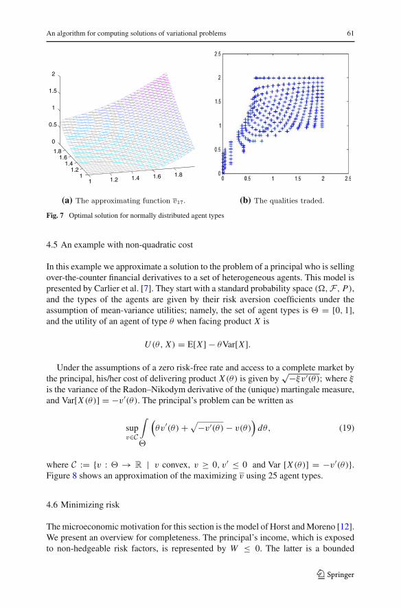
The weight assigned to each agent type is built into h and H , so the vector x remainsunchanged. We obtain Fig. 7.

Remark 4.1 It is interesting to see that in this case bunching of the second kind, asdescribed by Roché and Choné in [19], appears to be eliminated as a consequence ofthe skewed distribution of the agents. This can be seen in the non-linear level curvesof the optimizing function v, and it is also quite evident in the plot of the tradedqualities.

The codes for the two previous examples were run on Matlab 7.0.1.24704 (R14)in a Sun Fire V480 (4 × 1.2 HGz Ultra III, 16 GB RAM) computer running Solaris2.10 OS. In the first example 57.70 s of processing time were required. The runningtime in the second example was 81.72 s.

123


1 1.2 1.4 1.6 1.811.2

1.41.6

1.8

0

0.5

1

1.5

2

(a) (b)

Fig. 7 Optimal solution for normally distributed agent types

4.5 An example with non-quadratic cost

In this example we approximate a solution to the problem of a principal who is sellingover-the-counter financial derivatives to a set of heterogeneous agents. This model ispresented by Carlier et al. [7]. They start with a standard probability space (,F , P),and the types of the agents are given by their risk aversion coefficients under theassumption of mean-variance utilities; namely, the set of agent types is � = [0, 1],and the utility of an agent of type θ when facing product X is

U (θ, X) = E[X ] − θVar[X ].

Under the assumptions of a zero risk-free rate and access to a complete market bythe principal, his/her cost of delivering product X (θ) is given by

√−ξv′(θ); where ξ

is the variance of the Radon–Nikodym derivative of the (unique) martingale measure,and Var[X (θ)] = −v′(θ). The principal’s problem can be written as

supv∈C

∫

�

(θv′(θ) +√−v′(θ) − v(θ)

)dθ, (19)

where C := {v : � → R | v convex, v ≥ 0, v′ ≤ 0 and Var [X (θ)] = −v′(θ)}.Figure 8 shows an approximation of the maximizing v using 25 agent types.

4.6 Minimizing risk

The microeconomic motivation for this section is the model of Horst and Moreno [12].We present an overview for completeness. The principal’s income, which is exposedto non-hedgeable risk factors, is represented by W ≤ 0. The latter is a bounded

123


0 0.2 0.4 0.6 0.8 10

2

4

6

8

10

12

14

Fig. 8 The approximating function v25

random variable defined on a standard, non-atomic, probability space (,F , P). Theprincipal’s goal is to lay off parts of his/her risk with the agents whose preferencesare mean-variance. The agent types are indexed by their coefficients of risk aversion,which are assumed to lie � = [a, 1] for some a > 0. Notice that the variationalproblem that arises in this example is structurally different than the previous ones. Wehave included it to show that our method can be used in more general setting. Theprincipal underwrites call options on her income with type-dependent strikes:

X (θ) = (|W | − K (θ))+ with 0 ≤ K (θ) ≤ ‖W‖∞.

If the principal issues the catalogue {(X (θ), π(θ))}, he/she receives a cash amountof∫� π(θ)dθ and is subject to the additional liability

∫� X (θ)dθ . He/she evaluates

the risk associated with her overall position

W +∫

�

(π(θ) − X (θ))dθ

via the “entropic measure” of his/her position, i.e.

ρ

⎛⎜⎝W +

∫

�

(X (θ) − π(θ))dθ

⎞⎟⎠ ,

where ρ(X) = log(E[exp{−β X}]) for some β > 0. The principal’s problem is todevise a catalogue as to minimize his/her risk exposure. Namely, he/she chooses afunction v and contracts X from the set

{(X, v) | v ∈ C, v≤K1, −Var[(|W |−K (θ))+]=v′(θ), |v′|≤K2, 0≤K (θ)≤‖W‖∞},

123


in order to minimize

ρ

⎛⎜⎝W −

∫

�

{(|W | − F(v′(θ)))+ − E[(|W | − F(v′(θ)))+]} d

⎞⎟⎠− I (v),

where

I (v) =∫

�

(θv′(θ) − v(θ)

)dθ.

We assume the set of states of the World is finite with cardinality m. Each possiblestate ω j can occur with probability p j . The realizations of the principal’s wealth aredenoted by W = (W1, . . . , Wm). Note that p and W are treated as known data. Theobjective function of our non-linear program is

F(v, v′, K ) = log

⎛⎝exp

⎧⎨⎩−

n∑i=1

Wi pi + 1

n

n∑i=1

⎛⎝ n∑

j=1

T (K j − |Wi |)⎞⎠ pi

− 1

n

n∑i=1

⎛⎝ n∑

j=1

T (K j − |Wi |)⎞⎠ pi

⎫⎬⎭⎞⎠+ 1

n

∑vi − θ iv

′i

where K = (K1, . . . , Kn) denotes the vector of type dependent strikes. We denote byng the total number of constraints. The principal’s problem is to find

min(v,v′,K )

F(v, v′, K ) subject to G(v, v′, K ) ≤ 0,

where G : R3n → R

ng determines the constraints that keep (v, v′, K ) within the setof feasible contracts. Let (1/6, 2/6, . . . , 1) be the uniformly distributed agent types,

W = 4 ∗ (−2,−1.7, 1.4,−.7,−.5, 0) and

P = (1/10, 1.5/10, 2.5/10, 2.5/10, 1.5/10, 1/10).

The principal’s initial evaluation of his/her risk is 1.52. Figure 9 shows the plots for theapproximating v and the strikes. Note that for illustration purposes we have changedthe scale for the agent types in the second plot. The interpolates of the approximateto the optimal function v and the strikes are given in Table 1. After the exchanges withthe agents, the principal’s valuation of his/her risk decreases to −3.56.

Remark 4.2 Notice the “bunching” at the bottom.

123


0 0.2 0.4 0.6 0.8 10.5

1

1.5

2

2.5

3

3.5

4

4.5

5

5.5

(a)

1 2 3 4 5 60.7

0.75

0.8

0.85

0.9

0.95

1

1.05

1.1

(b)

Fig. 9 Optimal solution for underwriting call options

Table 1 The optimal function v

and the strikesv1 4.196344 K1 1.078869

v2 3.234565 K2 0.785079

v3 2.321529 K3 0.733530

v4 1.523532 K4 0.713309

v5 0.745045 K5 0.713309

v6 0.010025 K6 0.713309

5 Conclusions

In this paper, we have developed a numerical algorithm to estimate the minimizersof variational problems with convexity constraints, with our main motivation stem-ming from Economics and Finance. Ours is an internal method, so at each step theapproximate minimizers lie within the acceptable set of (convex) functions. This is ofparticular interest given our microeconomic motivation, where non-convex functionswould correspond to non-implementable contracts. Our examples are developed overone or two dimensional sets for illustration reasons, but the algorithm can be imple-mented in higher dimensions. However, it must be mentioned that, as is the case withthe other methods found in the related literature, implementing convexity has a highcomputational cost which increases geometrically with precision and exponentiallywith dimension.

A Appendix

In order to prove convergence of our algorithm we make use of the Convex Analysisresults contained in this section. We work on �, an open and convex subset of R

n andwe use the classical notation ∂ f (θ) to denote the subdifferential of f at θ . Recall that∂ f (θ) �= ∅ for any θ in the interior of the effective domain of f .

123


Definition A.1 A convex function f : � → R is said to be twice A-differentiableat a point θ0 ∈ C if ∇ f (θ0) exists and if there is a symmetric, positive definite matrixD2 f (θ0) (the Alexandrov Hessian of f at θ0), such that for any ε > 0 there isδ > 0 such that if ‖θ − θ0‖ < δ, then

supθ ∗∈∂ f (θ )

‖θ∗ − ∇ f (θ0) − D2 f (t0)(θ − θ0)‖ ≤ ε‖θ − θ0‖ (20)

The following theorem is due to Alexandrov [18]

Theorem A.2 Let f : � → R be convex, then it is almost everywhere twice A-dif-ferentiable on �. Moreover, if f is A-differentiable at θ0 ∈ B, then

limh→0

f (θ0 + h) − f (θ0) − 〈∇ f (θ0), h〉 − 12 〈D2 f (θ0)h, h〉

‖h‖2 = 0.

Corollary A.3 Let f : � → R be convex. Then the mapping

θ → ∇ f (θ)

is well defined and continuous almost everywhere.

Proof Let � be the set where f is twice A-differentiable. By definition ∇ f is welldefined on �, which is a set of full measure. When restricted to �, expression (20)can be written as

‖∇ f (θ) − ∇ f (θ0) − D2 f (t0)(θ − θ0)‖ ≤ ε‖θ − θ0‖,

which implies continuity of ∇ f . � The following is a well known property of convex functions. We were first made

aware of it by Carlier [5], but it probably dates back to Mosco or Joly (see for example[16]).

Proposition A.4 Let � ⊂ Rn be a convex, open set. Assume the sequence of con-

vex functions { fk : � → R} converges uniformly to f , then ∇ fk → ∇ f almosteverywhere on �.

Proof Denote by Di f the derivative of f in the direction of ei . The convexity offk and f implies the existence of a set B, with µ(�\B) = 0 such that the partialderivatives of fk and f exist and are continuous in B. Let θ ∈ B. To prove thatDi fk(θ) → Di f (θ), consider η such that θ + ηei ∈ �. Since fk is convex

fk(θ + hei ) − fk(θ)

h≥ Di fk(θ) ≥ fk(θ − hei ) − fk(θ)

h

for all 0 < h < η. Hence

fk(θ+hei )− fk(θ)

h−Di f (θ)≥ Di fk(θ)−Di f (θ)≥ fk(θ−hei )− fk(θ)

h−Di f (θ).

123


The left-hand side of this inequality is equal to

fk(θ + hei ) − f (θ + hei )

h+ f (θ) − fk(x)

h+ f (θ + hei ) − f (θ)

h− Di f (θ).

For ε > 0 let 0 < δ < η be such that

∣∣∣∣ f (θ + hei ) − f (θ)

h− Di f (θ)

∣∣∣∣ < ε (21)

for |h| ≤ δ. Let N ∈ N be such that

−εδ ≤ fn(θ) − f (θ) ≤ εδ,

n ≥ N . Hence, taking h = δ (notice that Eq. 21 still holds in this case), we have thatfor all n ≥ N ,

fn(θ + hei ) − f (θ + hei )

h≤ ε and

f (θ) − fn(θ)

h≤ ε.

Hence,

3ε ≥ Di fn(θ) − Di f (θ)

for all x ∈ B. The same argument shows that

−3ε ≤ Di fn(θ) − Di f (θ)

for all n ≥ N and all x ∈ B, which concludes the proof. �

Proposition A.5 Let � ⊂ Rn be a convex, compact set and let g : U → R be a

convex function such that for all θ ∈ �, the subdifferentials ∂g(θ) are contained in Qfor some compact set Q. Then there exists {g j : � → R} such that g j ∈ C1(�) andg j → g uniformly on �.

Proof Fix δ > 0 and define

�δ := {(1 + δ)x | x ∈ �}.

Extend g to be defined on �δ . Define

�(θ) :={

K e− 1

1−‖θ‖2 , ‖θ‖ < 1;0, otherwise.

123


Here K is chosen so that∫Rn �(θ)dθ = 1. For each ε > 0 define the mollifier

�ε(θ) := ε−n�(θ/ε) (for a discussion on the properties of mollifiers see, for exam-ple [11]). The functions

hε := g ∗ �ε

are convex, smooth and they converge uniformly to g on U as long as ε is small enoughso that

Uε := {θ ∈ �δ | d(x, ∂�δ) > ε}

is contained in �. Let n ∈ N be such that T1/n ⊂ �, then the sequence {g j := h1/j }has the required properties. � Lemma A.6 Consider φ(θ, z, p) ∈ C1(�×R× Q → R), where � = [a, b]n and Qis a compact convex subset of R

n. Let { fk : � → R} be a family of convex functionssuch that ∂ fK (θ) ⊂ Q for all θ ∈ �, and whose uniform limit is f . Let �k be theuniform partition of � consisting of kn cubes of volume µ(�k) := ( b−a

k )n. Denote byσ k

j , 1 ≤ j ≤ kn, be the elements of �k and let

µ(�k)

kn∑i=1

φ(θk

j , fk(θkj ),∇ fk(θ

kj ))

be the corresponding Riemann sum approximating∫� φ(x, fk(θ),∇ fk(θ))dθ , where

θkj ∈ σ k

j and σ kj ∈ �k . Then for any ε > 0 there is K ∈ N such that

∣∣∣∣∣∣∣∫

�

φ(θ, fk(θ),∇ fk(θ))dθ − µ(�k)

kn∑i=1

φ(θkj , fk(θ

kj ),∇ fk(θ

kj ))

∣∣∣∣∣∣∣≤ ε (22)

for any k ≥ K .

Proof By Lemma A.5, for each fk there exists a sequence of continuously differen-tiable convex functions {gk

j } such that

gkj → fk uniformly.

Let hk be the first element in {gkj } such that ‖hk− fk‖ ≤ 1

k and ‖∇hk(θ)−∇ fk(θ)‖ ≤ 1k

for all θ ∈ � where ∇ fk is continuous. Then hk → f uniformly, and by Lemma A.4we have that ∇hk(θ) → ∇ f (θ) a.e. It follows from Egoroff’s theorem that for everyn ∈ N there exists a set �n ⊂ � such that:

µ(�\�n) < 1/n and ∇hk → ∇ f uniformly on �n .

123


Let X σ kj(·) be the indicator function of σ k

j and define

gk(θ) := φ(θ, hk(θ),∇kk(θ)) −kn∑j=1

X σ kj(θ)φ(θk

j , hk(θkj ),∇hk(θ

kj )).

Fix n, consider θ0 ∈ �n and let {θk0} be the sequence of θk

j ’s converging to θ0 as the

partition is refined. By uniform convergence, ∇ f is continuous on �n , hence

limk→∞ hk(θ

k0) = f (θ0) and lim

k→∞ ∇hk(θk0) = ∇ f (θ0). (23)

It follows from (23) and the continuity of φ that gk → 0 almost everywhere on �n .Notice that as a consequence of the compactness of � and Q and the definition of hk

we have

‖φ(θ, fk(θ),∇ fk(θ))‖ ≤ K1, for all θ ∈ � and some K1 > 0,

and

∣∣∣∣∣∣gk(θ) −⎛⎝φ(θ, fk(θ),∇ fk(θ)) −

kn∑j=1

X σ kj(θ)φ(θk

j , fk(θkj ),∇ fk(θ

kj ))

⎞⎠∣∣∣∣∣∣ ≤ K2

k

for some K2 > 0 and all θ ∈ � where ∇ fk is continuous. Therefore

∣∣∣∣∣∣∣∫

�

φ(θ, fk(θ),∇ fk(θ))dθ − ‖σ kj ‖

kn∑i=1

φ(θkj , fk(θ

kj ),∇ fk(θ

kj ))

∣∣∣∣∣∣∣

≤ K2‖�‖k

+

∣∣∣∣∣∣∣∫

�

gk(θ)dθ

∣∣∣∣∣∣∣. (24)

By Lebesgue Dominated Convergence

limk→∞

∫

�n

gk(θ)dθ = 0,

moreover, the definition of �n implies

∫

�\�n

gk(θ)dθ ≤ 2K1

n.

123


Given ε > 0 take n ∈ N such that 2K1n ≤ ε

2 and K such that

K2‖�‖K

+

∣∣∣∣∣∣∣∫

�n

gK (θ)dθ

∣∣∣∣∣∣∣≤ ε

2.

Then Eq. (22) holds for all k ≥ K . �

References

1. Anguilera, N.E., Morin, P.: Approximating optimization problems over convex functions. Numer.Math. 111, 1–34 (2008)

2. Armstrong, M.: Multiproduct nonlinear pricing. Econometrica 64, 51–75 (1996)3. Bolton, P., Dewatripoint, M.: Contract Theory. MIT Press, Cambridge (2005)4. Brock, F., Ferone, V., Kawohl, B.: A symmetry problem in the calculus of variations. Calc. Var. Partial

Differ. Equ. 4, 593–599 (1996)5. Carlier, G.: Calculus of variations with convexity constraint. J. Nonlinear Convex Anal. 3(2), 125–143

(2002)6. Carlier, G.: Duality and existence for a class of mass transportation problems and economic applica-

tions. Adv. Mathe. Econ. 5, 1–21 (2003)7. Carlier, G., Ekeland, I., Touzi, N.: Optimal derivatives design for mean-variance agents under adverse

selection. Math. Finan. Econ. 1, 57–80 (2007)8. Carlier, G., Lachand-Robert, T., Maury, B.: A numerical approach to variational problems subject to

convexity constraints. Numer. Math. 88, 299–318 (2001)9. Choné, P., Le Meur, H.V.J.: Non-convergence result for conformal approximation of variational prob-

lems subject to a convexity constraint. Numer. Funct. Anal. Optim. 22(5), 529–547 (2001)10. Ekeland, I., Témam, R.: Convex analysis and variational problems. Classics in Applied Mathematics,

vol. 28. SIAM (1976)11. Evans, L.: Partial differential equations. Graduate Studies in Mathematics, vol. 19. American Mathe-

matical Society, Providence (2002)12. Horst, U., Moreno-Bromberg, S.: Risk minimization and optimal derivative design in a principal agent

game. Math. Finan. Econ. 2(1), 1–27 (2008)13. Kawohl, B., Schwab, C.: Convergent finite elements for a class of nonconvex variational problems. IMA

J. Numer. Anal. 18, 133–149 (1998)14. Lachand-Robert, T., Oudet, É.: Minimizing within convex bodies using a convex hull method. Siam

J. Optim. 16(2), 368–379 (2005)15. Lachand-Robert, T., Peletier, A.: Extremal points of a functional on the set of convex functions. In:

Proceedings of the American Mathematical Society, vol. 127–136, pp. 1723–1727 (1999)16. Mosco, U.: Convergence of convex sets and of solutions of variational inequalities. Adv. Math. 3,

510–585 (1969)17. Mussa, M., Rosen, S.: Monopoly and product quality. J. Econ. Theory 18, 301–317 (1978)18. Nicolescu, C., Persson, L.-E.: Convex Functions and their Applications. CMS Books in Mathematics.

Springer Science+Business Media, Heidelberg (2006)19. Rochet, J.-C., Choné, P.: Ironing, sweeping and multidimensional screening. Econometrica 66, 783–

826 (1988)

123

an algorithm for computing solutions of variational ... · an algorithm for computing solutions of...

Documents