1

An Agent-based Microeconomic Simulation of a local Market

Chris TroopEvangelos Milios

Faculty of Computer ScienceDalhousie University

Halifax, NS, B3H 1W5{troop,eem}@cs.dal.ca

Abstract

We describe an agent-based microeconomic simulation of a local market. Consumers and Sellers arerepresented as agents in the Aglets framework. Consumers follow a Cobb-Douglas utility function, andthey choose the seller that best matches their desired combination of goods and services. Different sellersprovide different combinations of goods and services. The amount of money available to consumers forspending depends on an external parameter representing the state of the economy. Sellers make profit i frevenues exceed costs. Although important aspects of a real economy, such as the total available moneysupply, the equilibrium between supply and demand, and the effect of the labour market, are not explicitlyrepresented in this simple model, they can be incorporated in the future. The advantages of an agent-basedsimulation are the following: global macroeconomic behaviors arise naturall y as a result of local agentinteractions; individual consumer and seller agents can become as sophisticated as desired (for example,spatial locations of consumers and sellers may influence consumer choice of a seller, or consumers canfollow an income and preference distribution that reflects a particular city), with no constraints imposed bytractabilit y of any mathematical models; the mobile agents (Aglets) framework allows a distributedimplementation of the economy over a network of workstations, thus allowing experiments on standardcomputing hardware with no requirement for access to a supercomputer. Future research wil l expand onthese advantages, to demonstrate the usefulness of the proposed framework for business planning (as a toolto answer what-if questions to a prospective seller), as a teaching tool in economics and business, and as aframework for electronic commerce, whereby real stores and real consumers are represented by agents,who carry out business transactions on their owners’ behalf.

2

1. Introduction

This paper describes an agent-based microeconomic simulation. Intelligent software

agents play the roles of buyers and sellers in a virtual marketplace. These agents are

imparted with realistic behaviors and goals. They are then introduced into an

environment where they behave and interact in an autonomous fashion. The results of the

simulation are the effects of their interaction.

The simulation is composed of four different agents. The primary agents in the

simulation are the Buyer and Seller agents. The Buyer is allotted an income for each

cycle. The Buyer is also imparted with preferences and a schedule of demand curves that

enable her to select a Seller and purchase goods from that Seller. The Seller agent

maintains a schedule of goods and prices. It presents a price index and value added index

to the Buyer. The Buyer uses these indices to select a Seller to do business with. The

third agent is the Controller agent. This agent permits the user to initialize the simulation.

The Controller also maintains an economic state, which the other agents will use as input

to make consumption decisions. There is only one Controller agent in the simulation at

any given time. The fourth and final agent is the Finder agent. It permits the other agents

to find the Sellers in the simulation. There is only one Finder agent in the simulation at

any given time. A more detailed description of the agents will be included in a later

section.

This report is organized in three sections with a conclusion. The background section will

outline conventional techniques used in economic simulations and modeling. It will also

include a more detailed description of agents and agent-based simulations and provide a

3

historical backdrop for this methodology. The background section will conclude with an

overview of related work in this area. The Simulation section wil l describe our model in

greater detail . It will provide a detailed description of the agents as well as the Buyers’

logic. The Future Work section will discuss the merits of the agent-based approach as

well as areas of potential research.

2. Background

Conventional economic models can be divided into two paradigms, static and dynamic.

The static model paradigm includes the graphical representations of supply and demand

found in virtually every introductory microeconomic textbook. Also included are single

equation and multiple equation models.

Dynamic models permit us to view the economy over time. This is the domain of

economic simulation. This is currently accomplished using one of two methods,

Dynamic multiple equation model and time series model. The following sections

describe these modeling techniques in greater detail.

Dynamic Multiple Equation Model

In this context, a simulation is a mathematical solution to a set of simultaneous equations.

These equations are known as difference equations. Pindyck and Rubinfeld define a

difference equation as an equation that “…relates the current value of one variable to

current and past values of other variables” . A set of these difference equations that can

be solved over time is known as a simulation model. The following is a classic

macroeconomic example of such a model. (Pindyck, 1981)

Ct = a1 + a2Yt-1

I t = b1 + b2(Yt-1 – Yt-2)Yt = Ct + I t + Gt

4

WhereY = gross national productC = consumptionI = investmentG = government spending

Time Series Model

Time series models are used to forecast future actions of a variable by making predictions

based on the past behavior of variables. As an example, an investor might predict the

future performance of a stock by evaluating how it performed in the past. Time series

models are useful when the use of a multi-equation model is no longer feasible. I.e. the

variables required for a multi-equation model may not have been recorded or the

relationships between the variables are unclear.

What is an agent?

The actual definition of a software agent is a matter of some debate. For our purposes we

will use the following description. (Lange)

“An agent is a software object that

1. Is situated within an execution environment2. Possesses the following mandatory properties3. Reactive: senses changes in the environment and acts according to those changes4. Autonomous: has control over its own actions5. Goal-driven: is proactive6. Temporarily continuous: is continuously executing7. And may possess any of the following orthogonal properties:8. Communicative: able to communicate with other agents9. Mobile: can travel from one host to another10. Learning: adapts in accordance with previous experience11. Believable: appears believable to the end user”

Agent-based Microeconomic Simulation

5

In an agent-based simulation intelligent software agents are used to play the roles of

participants in a complex economic system. In this case, agents act as buyers and sellers

in a virtual marketplace. These agents meet and engage in economic activities. This

system is able to simulate the “real world” by imparting the buyers and sellers with

realistic behaviors and goals. In an agent-based simulation we do not control the

simulation. We simply create the players and their environment and then allow them to

interact. Our results are the effects of their interaction. This enables the researcher to

create and observe a complex system while avoiding the difficulty of controlling it. Thus

avoiding the inherent complexity of a more mathematical methodology.

Related Work

The most recent example of this methodology is ASPEN. ASPEN is an agent-based

microeconomic simulation by Sandia National Laboratories. It makes use of intelligent

software agents to play the role of economic agents within a model of the US economy.

Microeconomic behaviors are combined to create macroeconomic results. ASPEN is

composed of household agents, firms, government and financial agents (banks and the

federal reserve).

Household consumption was not based on the maximization of a utility function, but

rather used ad hoc rules of thumb. For example, the demand for food was based on the

size of the household.

The model was used to test various federal monetary policies. The results were consistent

with accepted economic theory and practice (Basu, 1996).

3. The Simulation

6

Unlike the ASPEN model, which relied on ad hoc rules, this simulation relies on the

microeconomic theory of consumer choice. This theory models consumer-buying

behavior as a choice between two goods. This theory can be extended to model consumer

buying behavior as a choice between one good and all other goods (Varian, 1993). This

simulation models the choice consumers make between the physical good and the service

provided by the seller of the good. This simulation treats “service” as a good (not a bad)

that Buyers pay for. All Buyers value service. However, some value it more than others.

The Buyer makes a decision to spend X amount of his/her income on service and Y

amount of his/her income on physical goods.

Service can also be referred to as “value added”. Value added encompasses convenient

location, pleasant surroundings, convenient hours, knowledgeable staff, good after sale

service, etc… These are all costs that the Seller must incur and then recoup from the

buyers by charging higher prices.

3.1 Agents

3.1.1 Controller

The Controller agent controls the simulation. It directs the activities of the agents

involved in the marketplace. It also permits the user to initialize the marketplace.

Initialization refers to the process by which the user creates agents (buyers and sellers)

and provides them with behavioral attributes. The user is also permitted to alter the

simulation as it progresses. Sellers can be added or removed, and their pricing strategies

can be modified. There can be only one controller agent in the simulation.

The Controller enables user to initialize the agents in the simulation. Ιτ controls the

sequence of the simulation. (tells the Buyers to buy and the Sellers to report their status).

7

It also maintains an economic state that will be broadcast to the Buyers and Sellers in the

simulation. The economic state will affect their behaviors, in that a change in the

economic state will shift the Buyers’ demand curve. The Controller agent interacts with

the Buyers and the Sellers.

3.1.2 Buyer

The Buyer agents play the role of consumer within our virtual marketplace. The goal of

the Buyers is to purchase the preferred bundle of goods given their income and

preferences.

Each Buyer maintains a Cobb Douglas indifference curve as well as a demand curve for

each good in the simulation. Each Buyer also maintains an income. How the Buyer gets

this income is not part of our simulation (Although this increased sophistication could be

added). We simply give each Buyer an allotment of money at the beginning of each cycle

and the agent then spends the money according to her preferences. We assume that each

Buyer either works or receives some sort of social assistance as income. The Buyers

receive a message to shop from the controller agent and then communicate with then find

their ideal store by communicating with the Finder. Once their ideal Seller has been

found they purchase goods from this store. They may or may not spend all their money.

Buyer Choice

The Buyer chooses between services and goods. This choice between services and goods

leads to an optimal bundle (X, Y). Where X is the quantity of goods and Y is the quantity

of service.

Suppose the Buyer’s income per cycle is $10. And the buyer prefers $3 worth of service

and $7 worth of goods. We can treat this in percentage terms and say the Buyer prefers

8

30% of his/her income on service and 70% on durable goods. We can then treat these as

price and service indexes of .3 and .7 respectively.

Once the Buyer has decided upon his/her optimal bundle of goods/value added, he/she

must choose a Seller. The Seller presents the Buyers with two indices, a Price index and a

service index (may also be called value-added index).

The following table shows the price and service indices for three different sellers.

Seller 1 Seller 2 Seller 3

PI = .8 PI = .7 PI = .9

SI = .2 SI = .3 SI = .1

The Buyer looks at the sellers and we see that she will get her optimum combination of

price and service by buying from Seller 2.

Once the Buyer has chosen a Seller, he/she makes their purchases from that Seller given

their demand curve for each good. They purchase goods until they can make no more

purchases (may have money left over).

Different Buyers

Our simulation wil l involve the interaction of various types of Buyers. There will be three

basic types. 1) The frugal Buyer, he values low price over value added. 2) The average

Buyer, he values both price and value added. 3) The prestige Buyer, he is will ing to pay a

premium for value added. The type of buyer depends on the shape of their indifference

curve (indifference curves will be discussed in a later section).

3.1.3 Seller

Sellers play the role of Vendors in the virtual economy. Their goal is to maximize profits.

Profit = Revenue – Cost

9

Where…

Revenue = Price * QuantitySold

Cost = FixedCost + VariableCost * QuantitySold

VariableCost = UnitCost + CostOfValueAdded.

Price = UnitCost + UnitCost * Markup + UnitCost * ValueAddedIndex

In our simulation, the per unit cost of the good is the same for every Seller. However,

some Sellers have a higher variable cost due to the cost of delivering the Service (or

value added). Therefore, they must charge higher prices to recoup this loss. They may

also attempt to earn higher per unit profits.

All Sellers present a price and service index. If their service index is high their price

index will be low (high prices). The Sellers can also present a high price index (meaning

low prices) and a low service index (meaning little value added).

Each Seller maintains an inventory of goods. Just as the Seller’s income is external to the

simulation so is the production of good within the simulation. We assumed the Sellers

would purchase their goods from the same supplier. This way, all Sellers in this

economy have the same variable costs. The user is able to select what goods the Seller

will carry as well as how much the Seller will charge. The user is free to add or drop

goods from the Sellers product line at any time during the simulation. As well, the user is

able to alter the Seller’s pricing strategy. Altering the prices charged for the goods will

affect the Sellers price and value-added indices. Each Seller maintains these indices and

registers them with the Finder agent. This enables the Buyers to find the Seller with their

ideal bundle of goods and services. At the end of the cycle each Seller receives a “report”

message from the Controller. The Sellers then report their revenue, cost and profit to the

10

Controller. The Controller displays this information to the user. A Seller agent interacts

with the Controller, Finder and Buyer agents.

Types of Sellers

In their book, “Principles of Marketing” , Kotler, Armstrong and Cunningham (Kotler,

1999) identify three types of Sellers; self-service, limited-service and full -service. Our

simulation will make use of these distinctions. The self-service Seller provides minimal

value added but a low price. The limited-service Seller provides some value added at a

somewhat higher price. The full-service Seller provides high value added at a high price.

The self-service Seller accepts a lower margin than the full -service Seller does.

Under our model the self-service Seller will have a low value added index and a high

price index (this indicates low prices). The full-service Seller will have a high value

added index and a low price index (this indicates high prices).

3.1.4 Finder

The Finder agent allows the Buyer(s) and Seller(s) to meet in the virtual marketplace and

perform transactions. The Finder makes it possible for the Buyer(s) to find the Seller(s).

There can be only one Finder agent in the simulation. Once the Seller has been initialized

it registers itself with the finder agent. The Finder maintains references to all the Sellers

in the Economy. In this context Reference refers to the aglet id of each Seller agent. The

Finder acts as a “middle man” in our simulation by interacting with both Buyers and

Sellers.

3.2 Economic and Marketing Models

3.2.1 Buyer Behavior

11

The Buyers’ behavior within this simulation is modeled upon the microeconomic theory

of Consumer choice. The following is a brief description of this model.

3.2.2 The Budget Line.

The economic theory of consumer buying behavior assumes the buyer will attempt to

purchase the best bundle of goods they can afford (Varian, 1993). The selection of this

“best bundle” is dependent on the consumer’s preferences and budget. With this theory

we are able to reduce consumer behavior to a choice between two goods. The Consumer

chooses between good X and Y and decides on quantities Xi and Yi. Xi and Yi make up

the optimal bundle (Xi, Yi). This two good assumption may seem unrealistic at first.

However, we can treat one of the goods as representing all other goods the consumer may

want to consume. This good is known as a Composite good. This assumption greatly

simpli fies the graphical representation of this decision making process as well as future

calculations regarding this choice.

In choosing between two goods, the Buyer must decide what he/she is able to afford. This

requires the Budget Line. The Budget line can be represented in two-dimensional space.

The quantity of good one in measured on the horizontal axis and the quantity of good two

is measured on the vertical axis. The vertical intercept of this curve can be calculated by

dividing the Buyer’s income by the price of good 2. The Horizontal intercept can be

calculated by dividing the Buyers income by the price of good 2. A budget line is shown

in Fig 1.

12

Good 1

Goo

d 2

Horizontal intercep =income/price of good one.

Vertical intercept =income/price of good two

Fig 1.

3.2.3 Indifference Curve

13

The second part of the purchase decision involves what the Buyer wants, i.e. what

combination of good 1 and good 2 is the most desirable. This is done by examining the

Buyer’s indifference curve. The indifference curve maps the rate at which the buyer is

will ing to substitute good 1 for good 2. The indifference curve is generally a downward

sloping convex curve. The indifference curve shows all possible combinations of good 1

and good 2 that are equally satisfactory to the Buyer (Browning, 1992). The indifference

Curve is shown in Fig 2.

Good 1

Goo

d 2 Indifference Curve

Fig 2.

The Buyer is equally satisfied with any distribution along the indifference curve.

However, as the distribution moves down the indifference curve, the Buyer requires more

and more of good 1 to compensate him for a small loss of good 2. As the distribution

14

moves up the indifference curve the buyer requires more and more good 2 to compensate

him for a small loss of good 1.

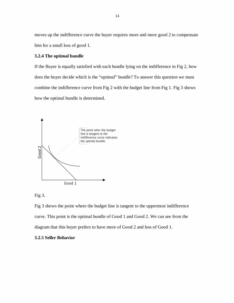
3.2.4 The optimal bundle

If the Buyer is equally satisfied with each bundle lying on the indifference in Fig 2, how

does the buyer decide which is the “optimal” bundle? To answer this question we must

combine the indifference curve from Fig 2 with the budget line from Fig 1. Fig 3 shows

how the optimal bundle is determined.

Good 1

Goo

d 2

The point wher the budgetline is tangent to theindifference curve indicatesthe optimal bundle.

Fig 3.

Fig 3 shows the point where the budget line is tangent to the uppermost indifference

curve. This point is the optimal bundle of Good 1 and Good 2. We can see from the

diagram that this buyer prefers to have more of Good 2 and less of Good 1.

3.2.5 Seller Behavior

15

Seller Behavior is modeled according to economic and marketing theories. An integral

part of the Seller’s behavior is the economist’s assumption of profit maximization. This

assumption does have its limitations. In the case of a small firm where the owner may

work in the firm profits may be traded off for increased leisure time. Or a firm may favor

the goals of social responsibil ity or increased market share (Mansfield, 1997). For our

purposes the goal of profit maximization will suffice. Another part of the Seller’s

behavior is the various business strategies the Seller can follow to achieve this goal. This

strategy is displayed by what kind of seller they are; self-service, limited-service or full -

service. Each Seller offers a different amount of value added to their good. The Buyer

pays for this value added by paying a higher price. The value added can be in the form of

convenient locations, good hours and increased customer service (Kotler, 1999).

The seller can take various forms. The discount seller is able to offer his goods at a low

price because he applies a small amount of value added to his goods. The average seller

offers his goods at a slightly higher price and offers a higher amount of value added. The

prestige seller offers the highest amount of value added and offers his goods at the

highest possible price.

4. Simulation Results

16

The simulation produced consistent results when initialized with a population of Buyers

and Sellers. The Buyers chose Sellers that were consistent with their preferences. As the

cost of providing value added changed (The price of value added increased or decreased)

some buyers would choose to shop at a different seller. We also found the aglets

framework to be extremely effective in modeling human behavior. Our Buyers use

conventional microeconomic theories of consumer behavior. It would also be possible to

take a more ad hoc approach and create a rules based system as proposed by researcher at

the first Workshop on Artificial Intelligence in Economics and Management (Hoffman,

1986).

5. Future Work

Economists have long used the distinction between microeconomics and

macroeconomics. Microeconomics focuses on the economic activities of the individuals

within an economy, and Macroeconomics analyzes the economy as a whole. Clearly this

is not an ideal starting point for the creation of a truly general economic theory. Present

macroeconomic theory does not suff iciently account for the heterogeneity of Agents (van

Ees, 1991) We feel that an agent-based framework can give macroeconomics in

particular and microeconomics in particular an individualistic foundation.

“There is no other more difficult branch of economics than dynamic economic models”

(Neal & Shone pg 124). The addition of time to an economic model greatly increases

complexity. The researcher must decide what time interval(s) will be used. With multiple

equation models each equation may require a different interval to achieve equil ibrium.

Also, an independent variable X at time t may require the calculation of a dependent

17

variable Y at time t – 1. Of course at time t – 1 Y it is an independent variable. It in turn

may require the calculation of variables at time t – 2, and so on. The researcher is then

forced to make assumptions to deal with these complications. These assumptions may

hinder the researcher’s quest for realism. In an agent-based model or simulation the

complexity of time is of no great concern. Each agent takes as much time as required to

perform her task as is required (as is the case in the real world). In fact it is the agent’s

abil ity to mirror the real world that makes it such a compell ing and (we think) useful tool

for researchers.

In our local market simulation the Buyer is required to choose a Seller that offers the

appropriate combination of goods and services. The next logical extension of this model

would be the addition of spatial constraints. Each agent in the economy would be given

an address and the location of the Seller would also be a part of the Buyers decision. Our

simulation was designed so this could be a feasible extension. Conventional multiple

equation models are ill equipped to deal with this added complication. There is the

possibility of using a gravity model to deal with a spatial environment. However, an

agent-based simulation could more easily reflect this reality. Agents could occupy a

location within an environment just as real-li fe Buyers and Sellers occupy a location.

We used the aglets framework to implement our local market simulation. Aglets are Java

objects that execute on a host. They are able to cease execution, store their state, transport

themselves to another host and resume execution. This capability makes an aglet a

Mobile Agent. Aglets also have the ability to send and receive messages. This makes the

18

aglet framework a powerful tool in modeling and simulation research. Whereas other

agent-based simulations might require powerful computational abil ity i.e. a super

computer. Aglets can be deployed on a network and the processing load can be

distributed over various hosts. The ASPEN project described in the Background section

of this paper ran on Sandia’s Paragon super computer. Our local market simulation is

able to run on a PC. As more agents are added to the simulation more PCs can be added

to the network to add processing capabil ity. The processing capacity required is

dependent on both the number and size of aglets within the simulation. Size referring to

the complexity of each aglet. Greater sophistication wil l lead to larger processing

requirements. This is somewhat of a subjective limitation. In that it is up to the researcher

to decide what is an acceptable length of processing time for each cycle. The network

paradigm could also be used to reflect the spatial reality of the marketplace being

modeled. Each workstation in the network could house the Buyers and Sellers of a

different neighborhood.

Macroeconomic fluctuations arise as a result of individual behaviors. Conventional

economics are ill equipped to deal with this reality. Modeling complex human behavior

within a mathematical framework is both conceptually and practically diff icult (Hoffman

et al. 1986) We believe that an agent based methodology would provide a more accurate

and easier to implement model of the real world. Buyers are represented by buyer agents.

Sellers are represented by seller agents. A central bank could be represented by a

banking agent, and so on. Researchers would no longer be required to represent an

economy (or part thereof) as a system of equations. This would also allow the researcher

19

to avoid the inevitable mathematical errors associated with the conventional multi-

equation approach.

Future research in this area is not limited to macroeconomic simulations. Our local

market simulation might be the first step in the replacement of the conventional gravity

model. The abil ity to model not only the spatial environment but the behaviors and

preferences of Buyers and Seller could make it interesting from a marketing or business

planning perspective. This local market simulation could also be extended to allow users

to create a buyer or seller agent to represent them and act on their behalf in this virtual

marketplace.

6. Conclusion

We conclude that software agents and the agent-based simulation methodology are valid

and useful tools for economic modeling. Even in its present state, our local market

simulation could prove interesting to those in the marketing and business community. It

could serve to answer various “what if questions” , as well as assist decision-makers in

selecting a product mix and pricing strategy.

Intuitively we know that macroeconomic phenomena arise as a result of individual

behaviors and activities. However, the micro-foundations of macroeconomics have

proven elusive with conventional mathematical modeling techniques. It is difficult for

researchers to model complex human behaviors within a mathematical framework.

20

This has forced economists to adopt the familiar microeconomic vs. macroeconomic

distinction. Software agents and agent-based simulations should permit economists to

soften this distinction, and provide an individualistic foundation to macroeconomics.

21

References

Basu N., R.J. Pryor, T. Quint and T. Arnold, (1996), ‘ASPEN: A Microsimulation Modelof the Economy’, Sandia National Laboratories, Albuquerque, New Mexico.

Browning Edgar K. and Jacquelene M. Browning, (1992) ‘Microeconomic Theory andApplications, Harper Collins’ .

Diamond Peter A., (1984) ‘A Search-Equilibrium Approach to the Micro Foundations ofMacroeconomics: The Wicksell Lectures’ , MIT Press, Cambridge.

Ees van Hans, (1991), ‘Macroeconomic Fluctuations and Individual Behaviour’ , GowerPublishing Company, Vermont.

Hansen Lars Peter and Thomas J. Sargent, (1991), ‘Rational Expectations Econometrics’ ,Westview Press, Boulder.

Hoffman Elizabeth, V. S. Jacob, James R. Marsden and Andrew Whinston, (1986),‘Artificial Intelligence in Economics—Expert Systems Modelling of MicroeconomicSystems’, From: ‘Artificial Intelligence in Economics and Management’ , Edited by L.F.Pau, North-Holland, New York.

Kotler Phil ip, Gary Armstrong, Peggy H. Cunningham, (1999), ‘Principles of Marketing’ ,Prentice Hall Canada Inc., Scarborough, Ontario.

Lange Danny B. and Mitsuru Oshima, ‘Programming and Deploying Java Mobile Agentswith Aglets’ , Addison-Wesley, Massachusetts.

Mansfield Edwin, (1997), ‘Microeconomics’ , WW Norton & Company, New York.

Neal F. and R. Shone, (1976), ‘Economic Model Building’ , The Macmillon Press Ltd.London.

Pindyck Robert S. and Daniel L. Rubinfeld, (1981), ‘Econometric Models andEconometric ForeCasts’ , second edition, McGraw-Hill Book Company, Toronto.

Varian Hal R., (1993), ‘ Intermediate Microeconomics’ , WW Norton & Company, NewYork.

Wichers Robert, (1996), ‘A Theory of Individual Behavior’ , Academic Press, Toronto.