an advanced subgrid-scale model for large eddy simulation ... · together with recent remarkable...

http://www.tytlabs.com/review/© Toyota Central R&D Labs., Inc. 2014 http://www.tytlabs.com/review/© Toyota Central R&D Labs., Inc. 2014

Research Report

11R&D Review of Toyota CRDL, Vol.45 No.4 (2014) 11-20

Special Feature: CAE and Simulation

Report received on Oct. 27, 2014

1. Introduction

Together with recent remarkable advances in computers, numerical methods and turbulence modeling, Computational Fluid Dynamics (CFD) has become one of the most useful tools for investigating engineering application problems and designing fluid machinery. Since in automobile engineering the fluid flow is mostly turbulent, simulating turbulence effects with high accuracy is important in order to predict the performance of fluid machines with sufficient reliability.

Large Eddy Simulation (LES) is a suitable approach to predicting such turbulent flows, which reproduces unsteady flow with turbulent fluctuations on computers. We developed a subgrid-scale (SGS) model(1) and a numerical method suited for practical LES, exhibiting high accuracy and high computational stability. Using these techniques, precise analysis of complex turbulent phenomena, e.g., unsteady vehicle aerodynamics,(2) aerodynamic noise generation,(3) and

the performance of the engine intake port(4) depending on the formation of turbulent vortices, has become possible.

On the other hand, the LES method is also an effective tool for predicting turbulent heat transfer and turbulent mixing of gas or liquid. In order to maintain high accuracy in simulations of such complex phenomena, an excellent SGS model for the thermal/passivescalar field as well as that for the velocity field is necessary. For this purpose, we have recently developed a new SGS model for the thermal field(5) in collaboration with Nagoya Institute of Technology. Since the proposed model automatically takes into account the effects of physical properties (Prandtl/Schmidt number), it is expected to be a refined and versatile SGS model for analyzing thermal and scalar fields. The Prandtl number is a dimensionless number indicating the ratio of kinematic viscosity to thermal diffusivity, and the Schmidt number is the ratio of kinematic viscosity to mass diffusivity. In the present paper, the construction of the proposed model

Computational Fluid Dynamics, Turbulent Flow, Heat Transfer, Large Eddy Simulation,Subgrid-scale Model, Boundary Layer, Turbulent Mixing, Heat Exchanger,

Manufacturing Process

A new subgrid-scale (SGS) model for Large Eddy Simulation (LES) of thermal field is proposed. The proposed model is an extended version of the mixed-time-scale SGS model for velocity field by Inagaki et al. (2005), where the hybrid time scale between the time scales of the velocity and thermal fields is introduced to represent the dissimilarity between the velocity and thermal fields. In addition, the wall-asymptotic behavior is satisfied by incorporating the wall-damping function for LES based on the Kolmogorov velocity scale by Inagaki et al. (2006).

The model performance is tested in plane channel flows at various Prandtl numbers of up to 95 and in the thermal entrance problem in a pipe flow. The results demonstrate that the superiority of the present model to the conventional Smagorinsky model and the dynamic Smagorinsky model, which is remarkable when using a coarse grid at a high Prandtl number. Since the proposed model is constructed with fixed model parameters, it does not suffer from the computational instability encountered with the dynamic model. Thus, the proposed model is confirmed to be a refined and versatile SGS model that is suited for practical LES of the thermal/passive scalar field. Using the proposed SGS model, LES of complex turbulent flows including heat and mass transfer as well as chemical reactions is expected to be more accurate and less expensive.

Masahide Inagaki

An Advanced Subgrid-scale Model for Large Eddy Simulation of Turbulent Heat and Mass Transfer

http://www.tytlabs.com/review/

12

© Toyota Central R&D Labs., Inc. 2014

R&D Review of Toyota CRDL, Vol.45 No.4 (2014) 11-20

described as follows:

(5)

(6)

(7)

where is the cube root of the grid-cell volume, the model parameters CMTS and CT are set to 0.025 and 10, respectively, and the vt is SGS eddy viscosity. Moreover, ( )^ denotes the space filtering operator with a filter width of 2 . Using the explicit filtering, the SGS kinetic energy is estimated as kes in Eq. (6), and

is used as the characteristic velocity scale in the SGS modeling. One advantage of this estimation is that the SGS eddy viscosity, vt , is consistently guaranteed to approach zero in the laminar-flow region because kes approaches zero by itself in this region.

Another essential point is that the timescale, tu, is defined as the harmonic average of tD and tS. The former stands for the characteristic timescale of the small scale motion corresponding to the cut-off scale, whereas the latter represents that of the large scales. Since the harmonic average changes the weight of the two timescales, the variation of vt according to the ratio of two timescales extends the applicability of the proposed model to a variety of flow fields.(1)

Moreover, since the proposed model consists of fixed model parameters, it does not suffer from numerical instability unlike the well-known dynamic Smagorinsky model. Note that Eq. (6) is slightly modified from the original equation. The modification is that a wall-damping function, fm , is supplemented for vt .

2. 2. 2 New Wall-damping Function Based on the Kolmogorov Velocity Scale

Although the original MTS model for velocity

field(1) does not follow the rigorous wall-asymptotic behavior of vt , i.e., vt ~ n3 (n: distance from the nearest wall), it does not lead to a reduction in the prediction accuracy for calculating velocity fields. Thus, the model essentially dispenses with the supplementation of an explicit wall-damping function. However, this shortcoming probably becomes discernible in the

and its validity are demonstrated.

2. Numerical Method

In LES, only the large energy-containing eddies are computed explicitly, whereas the effect of the unresolved subgrid scales is introduced using an SGS model. A space filtering is used to decompose the basis variables into grid-scale (GS) components, ( ) , and subgrid-scale (SGS) components, ( ) ' . For example, the GS velocity component is defined as follows:

(1)

where the integral is extended over the entire flow field, and Gi is a filtering function that serves to damp the spatial fluctuations with a shorter length than the filter width, Di. In practical use, a top-hat filter is usually applied.

2. 1 Space-filtered Basic Equations

The basic equations are obtained by applying the filtering operation to the Navier-Stokes, continuity, and energy (temperature transport) equations as follows:

(2)

(3)

(4)

where is the SGS stress tensor, and is the SGS heat flux vector, which

should be modeled. Here, the flow is assumed to be incompressible for simplicity.

2. 2 Subgrid-scale (SGS) Modeling

2. 2. 1 Mixed-timescale SGS Model for Velocity Field

The mixed-timescale (MTS) SGS model(1) that we proposed for tij is an eddy viscosity model, and is


13



(11)

(12)

(13)

where the model parameters CMTq and CTq are set to 0.042 and 10 (= CT), respectively. The at is the SGS eddy diffusivity for heat, and the damping function fl is obtained by Eq. (8) with A0 = 10.

Although a constant PrSGS (at = vt /PrSGS ) is often used for at , we avoid such a modeling in order to take into account the effect of Prandtl/Schmidt number. To attain that, a characteristic timescale of the thermal field, tG , is newly introduced, which is defined using an estimated SGS temperature fluctuation, kq . Here, kq is calculated using a space-filtering operator as when estimating kes. Finally, the timescale for at , tq , is given as the harmonic average of tu (timescale for velocity field) and tG in a similar manner to giving the timescale for vt . Consequently, the information on the thermal field is introduced into at , so that the proposed SGS model is applicable to flows with dissimilarity between velocity and thermal fields, e.g., flows at various Prandtl numbers.

3. Assessment of the SGS Model for Thermal Field in Basic Flows

3. 1 Fully Developed Channel Flow

3. 1. 1 Computational Conditions

The proposed SGS model is verified in plane channel flows at different Prandtl numbers. The computational condition and grid resolutions are shown in Table 1,where d is the channel half width. The Reynolds number based on the wall-friction velocity, Ret = dut /v, is set to 180, which corresponds to Rem = 2dum/v 5,600 defined using the bulk velocity. To examine the grid-dependency at the same time, we conduct several computations varying the number of grid points or the size of the computational domain. In Table 1, superscript + denotes the dimensionless value based on the wall-friction velocity and kinematic viscosity, v. In every case, the grid resolution in the wall-normal direction is sufficiently high. The no-slip condition is

calculation of a thermal field. In order to settle this problem, we developed a new wall-damping function(6) for LES as follows:

(8)

(9)

(10)

where the model parameters Cl and Ce are 4 and 0.835, respectively. Substituting the function f given by Eq. (8) for fm in Eq. (6), the modified MTS model satisfies the wall-limiting behavior, where A0 is set to 2. In addition, this function is also used in the thermal field modeling as shown later herein, which is more important to the accurate prediction of heat transfer at the wall surface.

Since this wall -damping function is based on the Kolmogorov velocity scale u'e instead of the wall-friction velocity that is conventionally used, its applicability is very high. The most important point in this function for LES is that the Kolmogorovvelocity scale u'e is estimated using a unique conversion method, i.e., multiplying , under the consideration of the grid dependency of eSGS. Consequently, we are able to obtain a proper wall-damping effect regardless of the grid resolution. Without the conversion method, the resultant damping effect strongly depends on the grid resolution used and the prediction accuracy becomes considerably worse.(6) Note that the distance from the nearest wall n needed in using the function is able to be easily computed by solving the following elliptic equation: ,where . The obtained wall-distance has a smooth distribution.(6) Alternatively, we can employ a calculation method(7) for a level set function that is often used for the simulation of interfacial flows.

2. 2. 3 Mixed-timescale SGS Model for Thermal Field

With the aid of the wall-damping function, we have constructed the MTS model(5) for thermal field as follows:


14



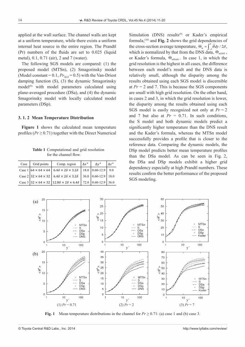
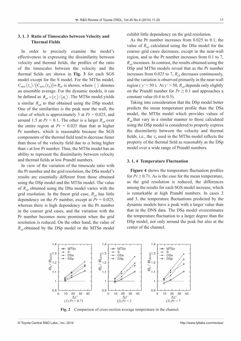
Simulation (DNS) results(9) or Kader’s empirical formula,(10) and Fig. 2 shows the grid dependencies of the cross-section average temperature, , which is normalized by that from the DNS data, ,or Kader’s formula, . In case 1, in which the grid resolution is the highest in all cases, the difference between each model’s result and the DNS data is relatively small, although the disparity among the results obtained using each SGS model is discernible at Pr = 2 and 7. This is because the SGS components are small with high grid resolution. On the other hand, in cases 2 and 3, in which the grid resolution is lower, the disparity among the results obtained using each SGS model is easily recognized not only at Pr = 2and 7 but also at Pr = 0.71. In such conditions, the S model and both dynamic models predict a significantly higher temperature than the DNS result and the Kader’s formula, whereas the MTSn model successfully provides a profile that is closer to the reference data. Comparing the dynamic models, the DSp model predicts better mean temperature profiles than the DSa model. As can be seen in Fig. 2,the DSa and DSp models exhibit a higher grid dependency especially at high Prandtl numbers. These results confirm the better performance of the proposed SGS modeling.

applied at the wall surface. The channel walls are kept at a uniform temperature, while there exists a uniform internal heat source in the entire region. The Prandtl (Pr) numbers of the fluids are set to 0.025 (liquid metal), 0.1, 0.71 (air), 2 and 7 (water).

The following SGS models are compared: (1) the proposed model (MTSn), (2) Smagorinsky model (Model constant = 0.1, PrSGS = 0.5) with the Van-Driest damping function (S), (3) the dynamic Smagorinsky model(8) with model parameters calculated using plane-averaged procedure (DSa), and (4) the dynamic Smagorinsky model with locally calculated model parameters (DSp).

3. 1. 2 Mean Temperature Distribution

Figure 1 shows the calculated mean temperature profiles (Pr ≥ 0.71) together with the Direct Numerical

Fig. 1 Mean temperature distributions in the channel for Pr ≥ 0.71: (a) case 1 and (b) case 3.

Table 1 Computational and grid resolution for the channel flow.

Case Grid points Comp. region

Case 1 18.0 0.60-12.9 9.0

Case 2 36.0 0.60-12.9 18.0

Case 3 72.0 0.60-12.9 36.0

(1) Pr = 0.71 (2) Pr = 2 (3) Pr = 7

(a)

(b)

(1) (2) 2 (3) 7y+ y+ y+

y+ y+ y+


15



exhibit little dependency on the grid resolution. As the Pr number increases from 0.025 to 0.1, the

value of Ruq calculated using the DSa model for the coarser grid cases decreases, except in the near-wall region, and as the Pr number increases from 0.1 to 7, Ruq increases. In contrast, the results obtained using the DSp and MTSn models reveal that as the Pr number increases from 0.025 to 7, Ruq decreases continuously, and the variation is observed primarily in the near-wall region ( y+ < 50 ). At y+ > 50, Ruq depends only slightly on the Prandtl number for Pr ≥ 0.1 and approaches a constant value (0.4 to 0.5).

Taking into consideration that the DSp model better predicts the mean temperature profile than the DSa model, the MTSn model which provides values of Ruq that vary in a similar manner to those calculated using the DSp model is considered to properly express the dissimilarity between the velocity and thermal fields, i.e., the tq used in the MTSn model reflects the property of the thermal field as reasonably as the DSp model over a wide range of Prandtl numbers.

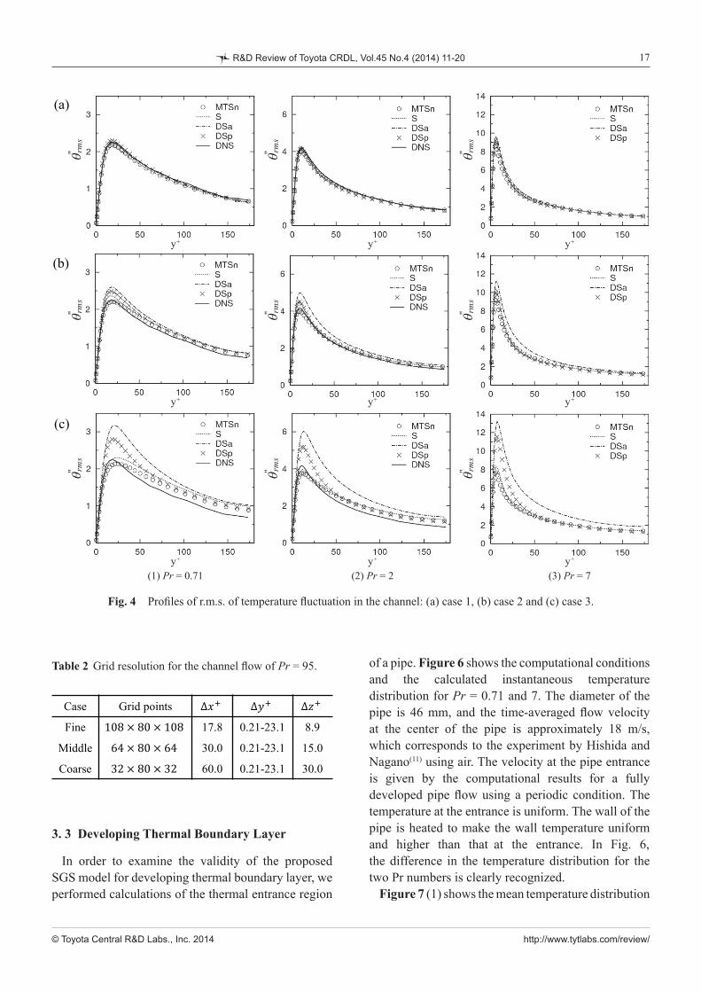
3. 1. 4 Temperature Fluctuation

Figure 4 shows the temperature fluctuation profiles for Pr ≥ 0.71. As is the case for the mean temperature, as the grid resolution is reduced, the differences among the results for each SGS model increase, which is remarkable at high Prandtl numbers. In cases 2 and 3, the temperature fluctuations predicted by the dynamic models have a peak with a larger value than that in the DNS data. The DSa model overestimates the temperature fluctuation to a larger degree than the DSp model, not only around the peak but also at the center of the channel.

3. 1. 3 Ratio of Timescales between Velocity and Thermal Fields

In order to precisely examine the model’s effectiveness in expressing the dissimilarity between velocity and thermal fields, the profiles of the ratio of the timescales between the velocity and the thermal fields are shown in Fig. 3 for each SGS model except for the S model. For the MTSn model,

is shown, where denotes an ensemble average. For the dynamic models, it can be defined as . The MTSn model yields a similar Ruq to that obtained using the DSp model. One of the similarities is the peak near the wall, the value of which is approximately 3 at Pr = 0.025, and around 1.5 at Pr = 0.1. The other is a larger Ruq over the entire region at Pr = 0.025 than that at higher Pr numbers, which is reasonable because the SGS components of the thermal field tend to decrease faster than those of the velocity field due to a being higher than v at low Pr number. Thus, the MTSn model has an ability to represent the dissimilarity between velocity and thermal fields at low Prandtl numbers.

In view of the variation of the timescale ratio with the Pr number and the grid resolution, the DSa model’s results are essentially different from those obtained using the DSp model and the MTSn model. The value of Ruq obtained using the DSa model varies with the grid resolution. In the finest grid case, Ruq has little dependency on the Pr number, except at Pr = 0.025, whereas there is high dependency on the Pr number in the coarser grid cases, and the variation with the Pr number becomes more prominent when the grid resolution is reduced. On the other hand, the value of Ruq obtained by the DSp model or the MTSn model

Fig. 2 Comparison of cross-section average temperature in the channel.

(1) Pr = 0.71 (2) Pr = 2 (3) Pr = 7(1) (2) 2 (3) 7Dz+ Dz+ Dz+


16



developed channel flow of technical oil (Pr = 95), which corresponds to the experiment by Neumann is performed. The Reynolds number, Rec = duc /v, is 10000, where uc is the velocity at the channel center. The grid resolutions are shown in Table 2.

Figure 5 shows the calculated temperature distributions. The results obtained using the MTSn model show better agreement with the experimental data and significantly lower grid dependency than the dynamic model, although some modification is introduced to the MTSn model. The proposed model has high applicability for a wide range of Prandtl number.

These better predictions of mean temperature and temperature fluctuation with the DSp model are attributed to the smaller Ruq , which leads to the larger at. This also confirms the validity of the timescale of the MTSn model for thermal field. As expected, the overestimations in the temperature fluctuation are well suppressed when using the MTSn model. The peak in the fluctuating temperature profiles obtained using the MTSn model is in best agreement with the DNS data regardless of the grid resolution employed.

3. 2 Channel Flow at a Very High Prandtl Number

In order to evaluate the proposed SGS model in very high Prandtl number fluids, the calculation of a fully

Fig. 3 Distributions of timescale ratio, Ruq in the channel: (a) case 1, (b) case 2 and (c) case 3.

(a)

(b)

(c)

(1) DSa (2) DSp (3) MTSny+ y+ y+

y+

y+

y+

y+

y+

y+


17



of a pipe. Figure 6 shows the computational conditions and the calculated instantaneous temperature distribution for Pr = 0.71 and 7. The diameter of the pipe is 46 mm, and the time-averaged flow velocity at the center of the pipe is approximately 18 m/s, which corresponds to the experiment by Hishida and Nagano(11) using air. The velocity at the pipe entrance is given by the computational results for a fully developed pipe flow using a periodic condition. The temperature at the entrance is uniform. The wall of the pipe is heated to make the wall temperature uniform and higher than that at the entrance. In Fig. 6,the difference in the temperature distribution for the two Pr numbers is clearly recognized.

Figure 7 (1) shows the mean temperature distribution

3. 3 Developing Thermal Boundary Layer

In order to examine the validity of the proposed SGS model for developing thermal boundary layer, we performed calculations of the thermal entrance region

Fig. 4 Profiles of r.m.s. of temperature fluctuation in the channel: (a) case 1, (b) case 2 and (c) case 3.

Table 2 Grid resolution for the channel flow of Pr = 95.

Case Grid points

Fine 17.8 0.21-23.1 8.9

Middle 30.0 0.21-23.1 15.0

Coarse 60.0 0.21-23.1 30.0

(1) (2) 2 (3) 7

(a)

(b)

(c)

'' rms

'' rms

'' rms

'' rms

'' rms

'' rms

'' rms

'' rms

'' rms

(1) Pr = 0.71 (2) Pr = 2 (3) Pr = 7y+ y+ y+

y+ y+ y+

y+ y+ y+


18



obtained using the proposed model for each section, and Fig. 7 (2) compares the predicted profiles of the Nusselt number along the streamwise direction with the experimental results for Pr = 0.71. The variation of mean temperature profiles in the streamwise direction is correctly reproduced by the proposed model. In addition, the obtained Nusselt number is in good agreement with the experimental data, whereas the dynamic model has less accuracy and less computational stability. The proposed model is confirmed to be a refined SGS model for thermal and passive scalar field.

4. Application to Engineering-relevant Problems

We have applied the developed SGS model to some engineering-relevant problems, e.g., thermo-fluid dynamics analysis of a heat exchanger. In order to realize a compact heat exchanger, the enhancement of heat transfer is usually necessary. As such, dimpled surfaces have been investigated in numerous studies. Moreover, some studies reported that a dimpled surface attains heat transfer enhancement over the increase of pressure drop. However, the mechanism of heat transfer enhancement by a dimpled surface and the relation between the pressure drop and the heat transfer remains unclear. In particular, the performance generally changes depending on the Prandtl number of the coolant. To investigate such phenomena, LES calculations using the proposed SGS model are

conducted. Figure 8 shows an example of an application to channel flows with a dimpled surface. The variation of the heat transfer enhancement with the Prandtl number is clearly explained.(12)

Another example is the thermo-fluid dynamics analysis of manufacturing processes with chemical reactions, in which the experimental measurement of the velocity and temperature distribution is difficult due to high temperature, and the

Fig. 5 Mean temperature distributions in the channel at Pr = 95.

Fig. 6 Computational condition and instantaneous temperature distribution for the thermal entrance problem in pipe.

Fig. 7 Computational results for the pipe flow.

Inflow (Fully-developed turbulent flow)

r x

Temperatureat inlet: Tin

Developing thermal boundary layer

D

Heat (Wall temperature: Tw)

Calculated instantaneous temperature distribution

low high

Pr = 0.71 (Air)

Pr = 7 (Water)

(1) DSa model (2) MTSn model(1) DSa model (2) MTSn modely+ y+

x/D = 1x/D = 1.9x/D = 3.9x/D = 5.9x/D = 14.9

(1) Mean temperature at each section (2) Nusselt number

11

1

(1) Mean temperature at each sectionr/R

(2) Nusselt numberx/D


19



rate with the main material concentration at the inlet is successfully estimated. Using the proposed simulation method, a low cost reactor may be designed, e.g., inlet gas concentration distribution (Fig. 11).

5. Conclusions

A new subgrid-scale model for the thermal/passive scalar field is proposed, which is an extended version of the mixed-timescale SGS model for the velocity field. In the proposed model, the hybrid timescale between the timescales of the velocity and thermal fields is introduced in order to represent the dissimilarity between the velocity and thermal fields. In addition,

concentration distribution of each component gas is even more difficult. Thus, the numerical prediction is an important tool for designing such a manufacturing process. Figure 9 demonstrates the computational result of Rayleigh-Benard convection caused by temperature difference of over 1000 K between the inflow gas and the heated wafer, which is encountered in a chemical vapor deposition reactor. This type of convection influences heat transfer, the deposition rate and their distributions at the wafer surface. As the rotation speed of the susceptor increases, the convection is suppressed, which can be predicted with sufficient accuracy. Figure 10 shows the predicted surface reaction rate.(13) The variation of the reaction

Fig. 11 Concentration distributions of material and by-product gases with inlet gas concentration distribution in a reactor.

Fig. 8 Prediction of heat transfer enhancement by dimpled surface.

Fig. 9 Rayleigh-Benard convection caused by temperature difference of over 1000 K between the inflow gas and the heated wafer in a CVD reactor.

Color map: Temperature distributions

Arrows: Velocity vectors

< Top view >

Heated wallOutlet

Inlet

Outlet< Side view >

lower higher

A A’

A A’

Color map: Concentration of by-product gasReaction surface

Color map: Concentration of main material gasReaction surface

Outlet Outlet

Dilute material gas Dilute material gasDense material gas

Fig. 10 Predicted surface reaction rate.

Inlet concentration of main material gas

Sur

face

reac

tion

rate Exp. Calc.

H

L Temperature

L

HVelocity

Flow

Temperature distribution

Enhanced cooling by turbulent vortices

Dimple

HeatCoolant / Air


20



Large Eddy Simulation Employing Kolmogorov Velocity Scale”, Int. J. of Heat and Fluid Flow,

Vol. 32 (2011), pp. 26-40.(7) Sethian, J. A., “A Fast Marching Level Set Method for

Monotonically Advancing Fronts”, Proc. of the Natl. Acad. of Sci. of USA, Vol. 93, No. 4 (1996),

pp. 1591-1595.(8) Germano, M., Piomelli, U., Moin, P. and Cabot, W. H., “A Dynamic Subgrid-scale Eddy Viscosity Model”,

Phys. of Fluids A, Vol. 3, No. 7 (1991), pp. 1760-1765.(9) Kim, J. and Moin, P., “Transport of Passive Scalars in

a Turbulent Channel Flow”, Turbulent Shear Flows 6 (1989), pp. 85-96.

(10) Kader, B. A., “Temperature and Concentration Profiles in Fully Turbulent Boundary Layers”, Int. J. of Heat and Mass Transfer, Vol. 24, No. 9 (1981), pp. 1541-1544.

(11) Hishida, M. and Nagano, Y., “Structure of Turbulent Temperature and Velocity Fluctuations in the Thermal Entrance Region of a Pipe”, Proc. of 6th Int. Heat Transfer Conference, Vol. 2 (1978), pp. 531-536.

(12) Sato, N., Kaneda, K., Inagaki, M., Horinouchi, N. and Ota, A., “Numerical Analysis of Unsteady Heat Transfer in a Simpled Channel Flow”, Proc. of 49th Natl. Heat Transfer Symp. of Japan (in Japanese) (2012), F313.

(13) Makino, S., Inagaki, M., Nakashima, K., Horinouchi, N., Kozawa, T. and Itoh, T., “Numerical

Simulation of Si Epitaxial Growth in a Vertical Rotating-disk Reactor”, Proc. of SCEJ 79th Annual Meeting (in Japanese) (2014), F220.

Table 1 and Figs. 1-4Reprinted from Int. J. of Heat and Fluid Flow, Vo. 34 (2012),pp. 47-61, Inagaki, M., Hattori, H. and Nagano, Y.,A Mixed-timescale SGS Model for Thermal Field at Various Prandtl Numbers, © 2012 Elsevier, with permission from Elsevier.

the wall-limiting behavior is satisfied by incorporating the newly developed wall-damping function for LES based on the Kolmogorov velocity scale.

The validity of the proposed SGS model is examined in canonical channel flows at various Prandtl numbers of up to Pr = 95 and in the thermal entrance problem for a pipe flow. The results reveal the superiority of the proposed model as compared to the conventional SGS models, which is remarkable when using a coarse grid at a high Prandtl number. Since the proposed model is constructed with fixed model parameters, it does not suffer from the computational instability encountered when using dynamic models in a complex geometry. Thus, the proposed model is confirmed to be a refined and versatile SGS model for thermal/passive scalar fields.

In addition, some applications to engineering-relevant problems were also presented. The LES of complex turbulent flows that include heat and mass transfer and chemical reactions is expected to be more accurate and less expensive using the proposed SGS model.

Acknowledgement

The application examples were prepared by Dr. N. Satoand Mr. S. Makino of TOYOTA CRDL, INC.

References

(1) Inagaki, M., Kondoh, T. and Nagano, Y., “A Mixed-time-scale SGS Model with Fixed Model-parameters for Practical LES”, J. of Fluids

Eng., Vol. 127, No. 1 (2005), pp. 1-13.(2) Sato, N., Kawakami, M., Kato, Y. and Inagaki, M., “LES Analysis of Flows Around a Simplified Car Model in Vertical Motions”, Proc. of 8th Int.

ERCOFTAC Symp. on Eng. Turbulence Modelling and Meas. (2010), pp. 424-429.

(3) Inagaki, M., Horinouchi, N., Ichinose, K. and Nagano, Y., “Predictions of Wall-pressure Fluctuation in Separated Complex Flows with Improved LES and Quasi-DNS”, Proc. of 3rd Int. Symp. of on Turbulence and Shear Flow Phenomena (2003), pp. 941-946.

(4) Inagaki, M., Nagaoka, M., Horinouchi, N. and Suga, K., “Large Eddy Simulation Analysis of Engine Steady Intake Flows Using a Mixed-time-scale Subgrid-scale Model”, Int. J. of Engine Res., Vol. 11, No. 3 (2010), pp. 229-241.

(5) Inagaki, M., Hattori, H. and Nagano, Y., “A Mixed-timescale SGS Model for Thermal Field at

Various Prandtl Numbers”, Int. J. of Heat and Fluid Flow, Vo. 34 (2012), pp. 47-61.

(6) Inagaki, M., “A New Wall-damping Function for

Masahide Inagaki Research Fields: - Analysis of Heat and Mass Transfer in Manufacturing Process and Cooling System - Computational Fluid Dynamics - Turbulence Modeling Academic Degree: Dr.Eng. Academic Societies: - The Japan Society of Mechanical Engineers - Japan Society of Fluid Mechanics - Heat Transfer Society of Japan Awards: - JSME Medal for Outstanding Paper, The Japan Society of Mechanical Engineers, 2003 - Best Author Award from JSIAM, The Japan Society for Industrial and Applied Mathematics, 2006

an advanced subgrid-scale model for large eddy simulation ... · together with recent remarkable...

Documents