an advance distributed control design for wide-area power...
TRANSCRIPT

AN ADVANCE DISTRIBUTED CONTROL DESIGN
FOR WIDE-AREA POWER SYSTEM STABILITY
by
Ibrahem E. Atawi
B.S., King Fahad University of Petroleum and Minerals, 2005
M.S., Florida Institute of Technology, 2008
Submitted to the Graduate Faculty of
the Swanson School of Engineering in partial fulfillment
of the requirements for the degree of
Doctor of Philosophy
University of Pittsburgh
2013

UNIVERSITY OF PITTSBURGH
SWANSON SCHOOL OF ENGINEERING
This dissertation was presented
by
Ibrahem E. Atawi
It was defended on
April 8, 2013
and approved by
Zhi-Hong Mao, Ph.D., Associate Professor, Electrical and Computer Engineering
Department
Gregory Reed, Ph.D., Associate Professor, Department of Electrical and Computer
Engineering
Ching-Chung Li, Ph.D., Professor, Department of Electrical and Computer Engineering
William Stanchina, Ph.D., Professor, Department of Electrical and Computer Engineering
Mingui Sun, Ph.D., Professor, Department of Bioengineering
Dissertation Director: Zhi-Hong Mao, Ph.D., Associate Professor, Electrical and Computer
Engineering Department
ii

Copyright c© by Ibrahem E. Atawi
2013
iii

AN ADVANCE DISTRIBUTED CONTROL DESIGN FOR WIDE-AREA
POWER SYSTEM STABILITY
Ibrahem E. Atawi, PhD
University of Pittsburgh, 2013
The development of control of a power system that supply electricity is a major concern in
the world. Some trends have led to power systems becoming overstated including the rapid
growth in the demand for electrical power, the increasing penetration of the system from
renewable energy, and uncertainties in power schedules and transfers. To deal with these
challenges, power control has to overcome several structural hurdles, a major one of which
is dealing with the high dimensionality of the system.
Dimensionality reduction of the controller structure produces effective control signals
with reduced computational load. In most of the existing studies, the topology of the control
and communication structure is known prior to synthesis, and the design of distributed
control is performed subject to this particular structure. However, in this thesis we present
an advanced model of design for distributed control in which the control systems and their
communication structure are designed simultaneously. In such cases, a structure optimization
problem is solved involving the incorporation of communication constraints that will punish
any communication complexity in the interconnection and thus will be topology dependent.
This structure optimization problem can be formulated in the context of Linear Matrix
Inequalities and `1-minimization.
Interconnected power systems typically show multiple dominant inter-area low-frequency
oscillations which lead to widespread blackouts. In this thesis, the specific goal of stability
control is to suppress these inter-area oscillations. Simulation results on large-scale power
system are presented to show how an optimal structure of distributed control would be
iv

designed. Then, this structure is compared with fixed control structures, a completely de-
centralized control structure and a centralized control structure.
Keywords: power system, control, distributed, inter-area oscillations.
v

TABLE OF CONTENTS
PREFACE . . . . . . . . . . . . . . . . . . . . . . . . . . . . . . . . . . . . . . . . . xii
1.0 INTRODUCTION . . . . . . . . . . . . . . . . . . . . . . . . . . . . . . . . . 1
2.0 LITERATURE REVIEW . . . . . . . . . . . . . . . . . . . . . . . . . . . . . 4
2.1 DIMENSIONALITY REDUCTION IN CONTROL OF A LARGE-SCALE
SYSTEM . . . . . . . . . . . . . . . . . . . . . . . . . . . . . . . . . . . . . 4
2.2 DAMPING CONTROL FOR INTER-AREA OSCILLATIONS . . . . . . . 8
3.0 OBJECTIVE . . . . . . . . . . . . . . . . . . . . . . . . . . . . . . . . . . . . 12
3.1 INTRODUCTION . . . . . . . . . . . . . . . . . . . . . . . . . . . . . . . . 12
3.2 DESIGN OF A HIERARCHICAL ARCHITECTURE OF CONTROL WITH
OPTIMAL TOPOLOGY . . . . . . . . . . . . . . . . . . . . . . . . . . . . 13
3.3 DEMONSTRATION OF THE HIERARCHICAL CONTROL SYSTEM . . 15
4.0 BACKGROUND . . . . . . . . . . . . . . . . . . . . . . . . . . . . . . . . . . 16
4.1 INTER-AREA OSCILLATIONS . . . . . . . . . . . . . . . . . . . . . . . . 16
4.1.1 Power System Modeling . . . . . . . . . . . . . . . . . . . . . . . . . . 16
4.1.2 Eigenvalues Stability Analysis . . . . . . . . . . . . . . . . . . . . . . 24
4.2 OPTIMIZATION TECHNIQUES . . . . . . . . . . . . . . . . . . . . . . . . 24
4.2.1 Linear Matrix Inequality . . . . . . . . . . . . . . . . . . . . . . . . . 24
4.2.2 `1-Minimization . . . . . . . . . . . . . . . . . . . . . . . . . . . . . . 26
5.0 DESIGN METHODS . . . . . . . . . . . . . . . . . . . . . . . . . . . . . . . 27
5.1 TASK I: FORMULATING AND SOLVING THE SYSTEM STABILIZA-
TION PROBLEM FOR VARIOUS CONTROL STRUCTURES . . . . . . . 27
5.1.1 System Model. . . . . . . . . . . . . . . . . . . . . . . . . . . . . . . . 28
vi

5.1.2 Controller Structure. . . . . . . . . . . . . . . . . . . . . . . . . . . . 28
5.1.3 Stabilization . . . . . . . . . . . . . . . . . . . . . . . . . . . . . . . . 30
5.2 TASK II: FORMULATING AND SOLVING THE SYSTEM STABILIZA-
TION PROBLEM UNDER COMMUNICATION CONSTRAINTS. . . . . . 32
5.2.1 Model Communication Channels . . . . . . . . . . . . . . . . . . . . . 32
5.2.2 Model of Augmented System . . . . . . . . . . . . . . . . . . . . . . . 34
5.2.3 Stabilization Problem . . . . . . . . . . . . . . . . . . . . . . . . . . . 35
5.3 TASK III: FORMULATING AND SOLVING THE STRUCTURAL OPTI-
MIZATION PROBLEM FOR CONTROL STRUCTURE SYNTHESIS . . . 36
5.3.1 Structural Optimization Problem . . . . . . . . . . . . . . . . . . . . . 37
5.3.2 Role of the Central Controller in the Hierarchy . . . . . . . . . . . . . 38
5.4 DESIGN OF OPTIMAL STRUCTURE . . . . . . . . . . . . . . . . . . . . 39
5.5 DEMONSTRATION OF CONTROL DESIGN METHODS . . . . . . . . . 40
6.0 SIMULATION RESULTS AND DISCUSSION . . . . . . . . . . . . . . . 42
6.1 SIMULATION RESULTS . . . . . . . . . . . . . . . . . . . . . . . . . . . . 42
6.1.1 Power System Description . . . . . . . . . . . . . . . . . . . . . . . . 42
6.1.2 Open-loop System Analysis . . . . . . . . . . . . . . . . . . . . . . . . 48
6.1.3 Designing Distributed Control . . . . . . . . . . . . . . . . . . . . . . 50
6.1.4 Optimal Design Simulation . . . . . . . . . . . . . . . . . . . . . . . . 59
6.2 DISCUSSION . . . . . . . . . . . . . . . . . . . . . . . . . . . . . . . . . . . 63
7.0 CONCLUSION . . . . . . . . . . . . . . . . . . . . . . . . . . . . . . . . . . . 70
APPENDIX. MORE SIMULATION RESULTS . . . . . . . . . . . . . . . . . 72
BIBLIOGRAPHY . . . . . . . . . . . . . . . . . . . . . . . . . . . . . . . . . . . . 84
vii

LIST OF TABLES
1 Decomposition of the IEEE 39-bus power system. . . . . . . . . . . . . . . . . 44
2 Generator, turbine, and governor parameters for the IEEE 39-bus system (per
unit). . . . . . . . . . . . . . . . . . . . . . . . . . . . . . . . . . . . . . . . . 45
3 Line parameters for the IEEE 39-bus power system (per unit). . . . . . . . . 46
4 Voltage and angle parameters for the IEEE 39-bus power system (per unit). . 47
5 Synchronizing torque coefficient between the buses (per unit). . . . . . . . . . 48
6 The eigenvalues, natural frequencies, and damping ratios for the optimal struc-
ture . . . . . . . . . . . . . . . . . . . . . . . . . . . . . . . . . . . . . . . . . 61
7 Control laws for the ten controllers. . . . . . . . . . . . . . . . . . . . . . . . 62
8 The eigenvalues, natural frequencies, and damping ratios for the centralized
structure. . . . . . . . . . . . . . . . . . . . . . . . . . . . . . . . . . . . . . . 77
9 The eigenvalues, natural frequencies, and damping ratios for the completely
decentralized structure. . . . . . . . . . . . . . . . . . . . . . . . . . . . . . . 78
10 The eigenvalues, natural frequencies, and damping ratios for open-loop system. 79
11 The eigenvalues, natural frequencies, and damping ratios for open-loop system
(cont.). . . . . . . . . . . . . . . . . . . . . . . . . . . . . . . . . . . . . . . . 80
viii

LIST OF FIGURES
1 (a) U.S. energy consumption by sector (data from [4]). (b) World renewable
electricity generation by source (data from [3]) . . . . . . . . . . . . . . . . . 2
2 Research contribution . . . . . . . . . . . . . . . . . . . . . . . . . . . . . . . 4
3 United Sates power network (figure adapted from [2]). . . . . . . . . . . . . . 5
4 Examples of dimensionality deduction methods for the sensory data. . . . . . 6
5 Northeast and midwestern U.S. states blackout of 2003. (Left satellite image)
shows light activity on August 14 at 9:29 p.m. EDT about 20 hours before
blackout. (Right satellite image) shows light activity on August 15 at 9:14
p.m. EDT about 7 hours after blackout (figure adapted from [1]). . . . . . . . 10
6 Block diagram of the Phasor Measurement Unit (figure adapted from [30]). . 11
7 (a) Centralized control structure in a large-scale power system. (b) Completely
decentralized control structure in a large-scale power system. . . . . . . . . . 12
8 Illustration of our design of distributed control structure in a large-scale power
system. . . . . . . . . . . . . . . . . . . . . . . . . . . . . . . . . . . . . . . . 14
9 The frequency and torque relation. . . . . . . . . . . . . . . . . . . . . . . . . 18
10 The frequency and power relation. . . . . . . . . . . . . . . . . . . . . . . . . 19
11 The frequency and load power relation. . . . . . . . . . . . . . . . . . . . . . 19
12 Block diagram of a power system. . . . . . . . . . . . . . . . . . . . . . . . . 21
13 (a) Two-area system. (b) Electrical equivalent. . . . . . . . . . . . . . . . . . 21
14 Block diagram of one area of an interconnected power system. . . . . . . . . . 22
15 Gain matrix structures of a (a) centralized (b) completely decentralized (c)
distributed control structure. . . . . . . . . . . . . . . . . . . . . . . . . . . . 29
ix

16 Block diagram of communication channel between subsystems. . . . . . . . . 33
17 IEEE 39-bus power system (figure adapted from [1]). . . . . . . . . . . . . . . 41
18 IEEE 39-bus power system decomposed into ten control areas. . . . . . . . . 43
19 Eigenvalues of the open-loop system. . . . . . . . . . . . . . . . . . . . . . . . 49
20 Open-loop system response to a non-zero initial condition in Areas 4 and 8. . 50
21 (a) The structure of the diagonal decision matrix YD. (b) The structure of the
full dimension decision matrix LD. . . . . . . . . . . . . . . . . . . . . . . . . 51
22 (a) YD solution matrix. (b) LD solution matrix. . . . . . . . . . . . . . . . . . 52
23 KD solution matrix resulting from step 2. . . . . . . . . . . . . . . . . . . . . 53
24 Feedback gain values in the KD matrix. . . . . . . . . . . . . . . . . . . . . . 53
25 Example of a fixed KD(i) matrix structure. . . . . . . . . . . . . . . . . . . . 54
26 (a) Example of the structure of the diagonal decision matrix YD(i). (b) Exam-
ple of the fixed structure of decision matrix LD(i). . . . . . . . . . . . . . . . 54
27 KD(i) matrix structure with actual feedback gain values. . . . . . . . . . . . 55
28 The variation in the dimensions of each of the ten controllers. . . . . . . . . . 56
29 The relationship between total control dimension, damping ratio, and energy
cost. . . . . . . . . . . . . . . . . . . . . . . . . . . . . . . . . . . . . . . . . . 57
30 Optimal feedback gain structure of distributed control. . . . . . . . . . . . . . 58
31 Communication channels assigned among the ten controllers. . . . . . . . . . 58
32 Eigenvalues of open and closed (optimal structure) loop system. . . . . . . . . 59
33 Control (optimal structure) system response to a non-zero initial condition in
Areas 4 and 8. . . . . . . . . . . . . . . . . . . . . . . . . . . . . . . . . . . . 60
34 Various control structures. . . . . . . . . . . . . . . . . . . . . . . . . . . . . 63
35 Controllers dimensions for all control structures. . . . . . . . . . . . . . . . . 64
36 Lowest five damping ratios. . . . . . . . . . . . . . . . . . . . . . . . . . . . . 65
37 Total control dimension vs. energy cost for different control structures. . . . . 66
38 Control (completely decentralized structure) system response to a non-zero
initial condition in Areas 4 and 8. . . . . . . . . . . . . . . . . . . . . . . . . 67
39 Control (”X” structure) system response to a non-zero initial condition in
Areas 4 and 8. . . . . . . . . . . . . . . . . . . . . . . . . . . . . . . . . . . . 67
x

40 Control (”Y” structure) system response to a non-zero initial condition in
Areas 4 and 8.. . . . . . . . . . . . . . . . . . . . . . . . . . . . . . . . . . . . 68
41 Control (”Z” structure) system response to a non-zero initial condition in Areas
4 and 8. . . . . . . . . . . . . . . . . . . . . . . . . . . . . . . . . . . . . . . . 68
42 Control (centralized structure) system response to a non-zero initial condition
in Areas 4 and 8. . . . . . . . . . . . . . . . . . . . . . . . . . . . . . . . . . . 69
43 Eigenvalues of the closed-loop (decentralized structure) system. . . . . . . . . 72
44 eigenvalues of the closed-loop (”X” structure) system. . . . . . . . . . . . . . 73
45 eigenvalues of the closed-loop (”Y” structure) system. . . . . . . . . . . . . . 74
46 Eigenvalues of the closed-loop (”Z” structure) system. . . . . . . . . . . . . . 75
47 Eigenvalues of the closed-loop (centralized structure) system. . . . . . . . . . 76
48 Feedback gain matrix structures during optimization development (part 1/3). 81
49 Feedback gain matrix structures during optimization development (part 2/3). 82
50 Feedback gain matrix structures during optimization development (part 3/3). 83
xi

PREFACE
My deep gratitude goes to Dr. Zhi-Hong Mao, who is my thesis supervisor. He has given
me so much support not only in research but also in my life. His motivation, perspective,
and hard work is appreciated, as it has enabled me to complete this thesis, and I am very
proud to have him as my research adviser.
I would also like to thank my committee members, Dr. Gregory Reed, Dr. Ching-Chung
Li, Dr. William Stanchina, and Dr. Mingui Sun, for all their suggestions and guidance.
Also, my deepest gratitude goes to my beloved Mrs. Hanouf Atawi for her support and
encouragement, and to my little two kids, Layan and Vayan. Moreover, my gratitude goes
overseas back home, Saudi Arabia, to my mother, brothers, and sisters for their support.
xii

1.0 INTRODUCTION
A power system is a small or large scale network that is used to supply and deliver electrical
power to residential and commercial consumers. The development of control of a power
system that supply electricity is a major concern in many countries such as the United
States and countries in Europe. Over the last five decades power systems have continued to
serve the growing needs of individuals and industry, but some trends in the filed of energy
supply have led to the current power system network becoming overstressed [65].
The first of these trends is the rapid, ongoing increase in the demand for electrical
power, as detailed in Figure 1a. In the U.S., from 2010 to 2035 the demand for electricity is
expected to grow by 22 percent from 3,877 billion kilowatt-hours to 4,716 billion kilowatt-
hours. Over the same period residential demand is expected to grow by 18 percent to
1,718 billion kilowatt-hours, and continued population shifts to climatically warmer regions
that will require power systems to accommodate greater cooling requirements . In 2035,
commercial demand is expected to increase by 28 percent to 1,699 billion kilowatt-hours.
From 2010 to 2035 transportation demand is expected to increase from 7 billion kilowatt-
hours to 22 billion kilowatt-hours. [3, 4]
The second trend that has led to the current power system network becoming overstressed
is the increasing penetration of energy from renewable sources such as wind and solar energy.
Wind energy constitutes the largest share of renewable energy, with expected increases from
99.7 billion kilowatts in 2005 to 1628.4 billion kilowatts in 2035 globally, as shown in 1b.
Also, both solar energy and biomass energy, while starting off slower than wind energy, are
expected to grow even more quickly. Overall, then, total renewable energy is expected to
grow quite rapidly in the short term. [3, 4]
1

Finally, electrical power is transferred considerable distances through high voltage trans-
mission systems, and these lines have flow limitations. Thus, there are large number of
sources of uncertainty in the operation of a power system, in terms of schedules and trans-
fers.
1980 1990 2000 2010 2020 2030 20400
5
10
15
20
25
30
35
Years
Qua
drill
ion
Btu
Delivered energy consumption by sector
ResidentialCommercialIndustrialTransportation
2005 2010 2015 2020 2025 2030 20350
500
1000
1500
2000
Years
Bill
ion
kWh
World renewable electricity generation by source
WindSolarGeothermalBiomass,Waste
Figure 1: (a) U.S. energy consumption by sector (data from [4]). (b) World renewable
electricity generation by source (data from [3])
To address these challenges, the power system network not only need to be upgraded
with advanced hardware and equipment, but also must be reconfigured to make it smarter –
capable of optimizing the use of the existing infrastructure while securing electrical service
that is reliable, economical, efficient, safe, and environmentally responsible [46]. In order to
2

achieve the aforementioned benefits that the smart grid provides, power control has to over-
come several structural hurdles, a major one of which is dealing with the high dimensionality
of the control system.
3

2.0 LITERATURE REVIEW
Dimensionality Reduction Techniques
Page 2
Power System Stability Concerns
System model
Sensory data
Controller structure
Frequency Voltage
Power System Control
Research Contribution
Inter-area oscillation
Figure 2: Research contribution
2.1 DIMENSIONALITY REDUCTION IN CONTROL OF A
LARGE-SCALE SYSTEM
In the United States the power grid is a huge interconnected network, as shown in Figure 3.
The North American network has between 10,000 and 100,000 nodes or branches and about
100 control centers [43]. The mathematical description of this network involves differential
and algebraic equations with extraordinarily high dimensional variable space [76]. The net-
work also requires the coordination of a large number of local actions on the part of the
energy generation and transmission controllers [29]. Furthermore, this network exhibits a
large range of characteristics, some which are highly nonlinear, such as bifurcation and chaos
4

[89]. These nonlinearities are generally hard to handle in control, even after simplification in
modeling [61]. Moreover, a large-scale power system needs to be controlled under condition
of distributed disturbances caused by noise and transmission delays scattered throughout
the network.
Figure 3: United Sates power network (figure adapted from [2]).
In control of a complex network, such as a large-scale power system, dimensionality
reduction become essential to the computation of control signals in real time. The purpose
of dimensionality reduction is to promote the efficiency and robustness of the power system by
reducing the computational and communicational complexity of the control. Dimensionality
reduction can be implemented for (i) the sensory data, (ii) the system model, and (iii)
controller structure, respectively.
Dimensionality reduction of the sensory data aims to transform date of high dimen-
sionality into a meaningful representation exhibiting reduced dimensionality, as shown in
Figure 4. Techniques commonly used to achieve this goal include linear methods such as
principle component analysis (PCA) [49] and multidimensional scaling (MSD) [28]. Exam-
ples of nonlinear methods are isomap [88], kernel (PCA) [83], diffusion maps [59], locally
liner embedding [80], locally linear coordination [87], Laplacian eigenmaps[12], and manifold
charting [19]. Sensory-data dimensionality reduction can also be achieved by directly reduc-
5

Figure 4: Examples of dimensionality deduction methods for the sensory data.
ing the number of sensory channels or sampling rates. For example, in power system design,
many research efforts have been made to determine optimal minimum sensor placements in
the network [13, 21, 40, 75]. To reduce the sampling rate, a novel sampling, paradigmcom-
pressive sensing, has been proposed, given that it can recover certain signals from far fewer
samples than traditional methods can [22, 23, 33]. For data collection in networked control
systems, compressive sensing can be realized in a decentralized manner [41, 10].
Dimensionality reduction of the system model aims to replace the original model with
one of a much smaller dimension. The reduced model should be a sufficiently accurate
approximation of the original model. One category of model-reduction methods is based
on identifying and preserving certain modes of interest [24], e.g. modal model reduction
[5, 16, 63]. Another category of these methods focuses on the observability and control-
lability properties of the system and is based on singular value decomposition (SVD) [7],
e.g., balanced truncation [66] and Hankel norm approximation [47]. In addition, moment
matching methods based on Krylov subspaces have been used for model reduction [6, 11, 24].
6

This thesis will focus only on the dimensionality reduction of the controller structure.
This reduction technique aims to produce effective control signals with reduced computa-
tional load. In comparison with entirely centralized control, completely decentralized control
has been a more popular choice of control architecture because of its ability to effectively
solve the problems of dimensionality, uncertainty, and information structure constraints in
large-scale systems [45]. Completely decentralized control most likely requires the weak inter-
connection assumption used in a large-scale network. A large body of existing literature has
contributed to the development of distributed control for large-scale systems [48, 84, 91, 93].
In particular, the optimal design of distributed control has been widely studied since at least
the 1970s [42, 81, 82]. In recent years, a trend has been to converge control, communication,
and computation in the design of a distributed structure for networked control systems [8].
However, in most of the existing research, the topology of the control and communication
structure are known prior to synthesis, and the optimal design for distributed control is
performed subject to this particular structure. To the best of our knowledge, only Langbort
and Gupta [55] have designed the controller and the topology the controller structure at the
same time.
min
∫ ∞0
XTQX + UTRU
subject to (2.1)
xi(t) = Aixi(t) +Biui(t) ∀t > 0, ∀i = 1, . . . , N
xi(0) = x0i
These researchers formulated the controller design as a linear quadratic regulation (LQR)
problem, in which communication was indirectly reflected in their problem formulation by a
topology dependent matrix in the LQR cost function, as shown in Equation (2.1). However,
the effect of these communication constraints in control cannot be objectively and quantita-
tively evaluated. In this thesis, we will study the synthesis problem in the control structure
and explicitly model the communication channels, considering time delay and uncertainties,
and directly defining, in the cost function, a term that punishes communication complexity
7

within the controller structure. We will transform the structural optimization problem into
a problem which seeks sparse solutions that can be solved using `1-minimization [32].
2.2 DAMPING CONTROL FOR INTER-AREA OSCILLATIONS
Power systems have a large number of generators and controllers, as well as many types
of loads. The entry of more controllers and loads increase the complexity and nonlinearity
of a power system. As a result, power systems are viewed as complex nonlinear systems
that are vulnerable to a number of instability problems. In power systems, we can classify
instability problems into three main types: voltage, phase, and frequency related problems
[27, 31, 54, 56, 57, 58, 62, 71, 77, 79]. These instability problems may be studied separately
for large-scale power systems. In this thesis, we will only focus on subclass of phase angle
related instability problems.
The ability of synchronous machines in an interconnected power system to remain syn-
chronize after being subjected to small disturbances is known as small signal stability, a type
of phase angle instability problem. The performance of an interconnected power system de-
pends on machine capability in order to maintain equilibrium between the electromagnetic
torque and mechanical torque of synchronous machines. The unbalanced between electro-
magnetic torque and mechanical torque can be maintained into two mechanisms:
• A synchronizing torque component in phase with rotor angle deviation. The lack of
sufficient synchronizing torque results in non-oscillatory instability.
• A damping torque component in phase with speed deviation. The lack of damping torque
results in low frequency oscillations.
make space
8

The main reason for oscillations in the power system is the unbalance between power
demand and available power, which in turn causes an unbalance between electromagnetic
torque and mechanical torque. Increasing and decreasing phase angle with a low frequency
will be reflected in the goal of maximum power transfer and optimal power system secu-
rity. Low frequency oscillations are generator rotor angle oscillations that have a frequency
between 0.1 -2.0 Hz and are classified based on the source of the oscillation [54, 72] as follows:
• Local oscillation: This occurs because of the swinging of generators at power station
against the rest of the power system, and happens to a small part of the power system.
Normally, the range of the frequency is 1-2 Hz.
• Inter-area oscillation: This occurs because of the swinging of many generators in one part
of power system against other generators in different parts of power system. Normally,
the range of the frequency is 0.1-1 Hz.
In addition to these types of oscillation, there can be other types associated with the
controllers, and are the result of poor design controllers [72]. Since the 1960s and 1970s,
the conventional controllers for oscillation damping control include the automatic voltage
regulator (AVR) [14], the power system stabilizer (PSS) [15], the speed governor [74], and
the field excitation control [52]. These controllers are single-input single-output (SISO)
controllers and work in a completely decentralized control structure. In a large-scale power
system, the inter-area frequencies may fall well below 0.2 Hz while local oscillations may
exceed 4 Hz [50]. Conventional SISO controllers cannot handle such a wide frequency range;
consequently, many incidents related to low frequency oscillations have been reported [70].
For example, as a result of an incidence of LFO on August 14, 2003, a massive power outage
occurred throughout eight northeastern and midwestern U.S. states, as well as Ontario,
Canada, as shown in Figure 5.
In recent years, wide-area measurement systems (WAMS) using synchronized phase mea-
surement units as shown in Figure 6 have been introduced into the design for damping control
[25, 30, 34, 35, 51, 64, 68, 69, 95, 96]. Wide-area measurement systems with PMU have made
it possible to implement centralized [92] and hierarchical control [34, 44, 51, 69] for oscil-
lation damping. However, in all of the studies mentioned above, the structure of damping
9

Figure 5: Northeast and midwestern U.S. states blackout of 2003. (Left satellite image)
shows light activity on August 14 at 9:29 p.m. EDT about 20 hours before blackout. (Right
satellite image) shows light activity on August 15 at 9:14 p.m. EDT about 7 hours after
blackout (figure adapted from [1]).
control is fixed, and the controller design is subjected to a fixed structure. In this thesis, we
present and demonstrate a hierarchical control system and control-communication co-design
for hundling inter-area oscillations in the damping control. Our controller structure has the
advantages of being synthesizeable and optimizable, taking into consideration of the cost
due to communication delays and data losses.
10

ABB Review 1/2001 59
data samples, positive-sequence voltages
and currents are calculated [1] and time-
stamped so that the exact microsecond
when the phasor measurement is taken
is permanently attached to it. The device
assembles a message from the time
stamp and the phasor data in a format
defined in IEEE standard 1344 [2], which
can then be transmitted to a remote
site over any available communication
link. Positive-sequence phasor data from
all substations equipped with such
devices are collected at an appropriate
central site using a data concentrator
or exchanged between local units for
protection/control applications.
Collecting and collating these measure-
ments provides a basis for new, very
powerful techniques for monitoring,
protecting and controlling power
networks.
Communication issues
Different technologies
Communication of the time-stamped
measurements to the data concentrator
is critical to the implementation. While
time is distributed to the PMUs through
an intricate network of satellites, present
devices utilize telephone, digital serial
and ethernet communications
technologies to provide the connection
to the data concentrator. The different
technologies involved in the communi-
cations infrastructure include direct
wiring, licensed and unlicensed radio
networks, microwave, public telephone,
cellular telephone, digital wireless, plus
combinations of these technologies.
Synchrophasor format
IEEE Standard 1344 [2] defines the
formats for output files provided by the
Phasor Measurement Units. Two files
(Header and Configuration) are defined
for setting up and assisting in
interpreting the phasor data, as well as
the format for the real-time binary output
file consisting of phasors and the time
stamp, which comprise the principal
output of the PMUs. The standard has
been of great help in ensuring that all
future applications of the synchronized
phasor measurements are able to access
the phasor data provided by PMUs from
different manufacturers.
Power system applications
The synchronized phasor measurement
technology is relatively new, and
consequently several research groups
around the world are actively developing
applications of this technology. It seems
clear that many of these applications can
be conveniently grouped as follows:
■ Power system monitoring
■ Advanced network protection
■ Advanced control schemes
2
Analoginputs
Anti-aliasingfilters
Phasormicro-
processor
GPSreceiver
Phase-lockedoscillator
A/Dconverter
Modems
Block diagram of the Phasor Measurement Unit1
SystemControl, protectionfunctionsArchival database
Advancedapplicationsoftware
PMU
PMU
PMU
PMU
DataConcentratorand collator
PMU utilization in a power system2
Figure 6: Block diagram of the Phasor Measurement Unit (figure adapted from [30]).
11

3.0 OBJECTIVE
3.1 INTRODUCTION
Figure 7: (a) Centralized control structure in a large-scale power system. (b) Completely
decentralized control structure in a large-scale power system.
The control structure for a complex network such as a large scale power system can be
classified as one of three main structures: a centralized structure, a completely decentralized
structure, or a distributed structure. Centralized control, as shown in Figure 7a, would entail
having a single controller measure all outputs of the power system, compute all the optimal
12

control input, and apply this control to all areas in one optimization problem. For a large-
scale system such as a power system, it would be decidedly unreasonable to implement a
centralized controller. A completely decentralized control system employs a single controller
for each area with no communication between individual controllers as shown in Figure 7b.
In this type of system, controllers ignore the interaction between the different subsystems.
This type of structure may contribute to insufficient performance in power system control,
especially if those subsystems are required to cooperate significantly in an interconnected
power system. The third structure, distributed control, also involves a single controller for
each subsystem, but, unlike the completely decentralized system, allows these subsystems to
communicate with each other by sharing information.
Significantly in terms of, a large scale network such as a power system requires reducing
the dimensionality inherent in the centralized configuration while avoiding the poor perfor-
mance that can result from utilizing a completely decentralized configuration. This fact,
along with the previously mentioned continuing increase in demand for electricity and the
growing incorporation of renewable energy into the power system, has led many researchers
to focus on distributed control in their search for a faster performing, more efficient control
structure for large-scale power systems.
3.2 DESIGN OF A HIERARCHICAL ARCHITECTURE OF CONTROL
WITH OPTIMAL TOPOLOGY
The main innovation of this section consists of reducing the dimensionality of control via
minimizing the topology of the control and communication network needed to achieve a
particular control goal. In most existing studies of hierarchical control, the interconnection
topology is fixed. In our thesis, the distributed controllers and their connection topology
are designed at the same time. Our structure optimization problem integrates control and
communication in the design. Our hierarchical control architecture has two layers, as shown
in Figure 8. The first layer is the decentralized layer, consisting of a distributed local
controller similar to that which is presented in Figure 7b. However within the layer the
13

Figure 8: Illustration of our design of distributed control structure in a large-scale power
system.
local controllers are allowed to connect and cooperate with one another. The connection
structure of these controllers is a part of the design and needs to be determined by solving
a structure optimization problem that involves incorporating a communication constraint,
which will punish any communication complexity in the interconnection and thus will be
topology dependent. This structure optimization problem can be formulated in the context
of Linear Matrix Inequalities [18] and `1-minimization [32].
The second layer of our design is a single central controller, similar to the one presented
in Figure 7a. However, the central controller in our method does not control the actuators
directly. Rather, it supervises and coordinates the operation of the local controllers in the
14

first layer, adaptively optimizing the control and communication structure in real time. As
a result, this central controller has greatly reduced responsibilities for control of the entire
system.
3.3 DEMONSTRATION OF THE HIERARCHICAL CONTROL SYSTEM
In terms of the stabilization problem of the power system, the specific goal of stabilization is
to suppress inter-area low frequency oscillations. Conventional controllers for power system
stabilization include an automatic voltage regulator (AVR) [14], a power system stabilizer
(PSS) [15], a speed governor [74], and a field excitation control [52]. These controllers are
single-input single-output (SISO) linear controllers and work in a completely decentralized,
non-cooperative manner; as a result, they cannot always guarantee stability when severe
disturbances occur in the power system. Our solution utilization is a hierarchical control
system that implements wide-area monitoring and control. Communication constraints will
be considered to determine optimal connections among the local controllers. We compare
the performance of our design with those having conventional designs and centralized control
under communication constraints.
15

4.0 BACKGROUND
4.1 INTER-AREA OSCILLATIONS
4.1.1 Power System Modeling
In designing, an optimal topology of distributed control to suppress inter-area low frequency
oscillation, we performed the steps presented here to obtain a dynamic model of a large scale
power system. The notation is borrowed from [53]. When there is an unbalance between the
mechanical torque (Tm) and electromagnetic torque (Te), the net torque causing acceleration
(or deceleration) is
Ta = Tm − Te (4.1)
where
Ta: acceleration motion torque N ·m.
Tm: mechanical torque N ·m.
Te: electromagnetic torque N ·m.
In the above equation, Tm and Te are positive for a generator and negative for a motor.
The combined inertia of the generator and prime mover is accelerated by the unbalance of
the applied torques. Hence, the equation of motion is
Jdωm
dt= Ta = Tm − Te (4.2)
where
J : the combined moment of inertia of the generator and turbine, kg ·m2.
ωm: the angular velocity of the rotor, rad/s.
16

The above equation can be normalized in terms of per unit inertia, using the constant H,
defined as the kinetic energy in watt-seconds at the rated speed divided by the VA base.
Using ωom to denote the rated angular velocity in mechanical radians per second, the moment
of inertia J in terms of H is
J =2H
ω20m
V Abase. (4.3)
Substituting the above in Equation (4.2) gives
2H
ω20m
V Abasedωm
dt= Tm − Te. (4.4)
If Tbase = V Abase
ω0m, rewriting the above equation yields the following:
2Hd(ωm/ω0m)
dt=Tm − TeTbase
= Tm − T e (4.5)
where Tm and T e are mechanical and electrical torque per unit (p.u.), respectively.
In the above equationωm
ω0m
=ω/pfω0/pf
=ω
ω0
= ω (4.6)
where ω is the angular velocity of the rotor in electrical rad/s, ωo is its rated value, and pf
is the number of filed poles.
Now we can rewrite Equation (4.5) as follows:
2Hdω
dt= Tm − T e. (4.7)
If δ is the angular position of the rotor in electrical radians with respect to a synchronously
rotating reference and δ0 is its value at t = 0,
δ = ωt− ω0t+ δ0. (4.8)
17

Taking the time derivative of the above equation, we have
dδ
dt= ω − ω0 = ∆ω. (4.9)
Based on Equation (4.6), we can write the above equation as
1
ω0
dδ
dt= ∆ω. (4.10)
Subsequently, the per unit equations of motion of a synchronous machine can be written as:
dω
dt=
1
2H(Tm − T e) (4.11)
dδ
dt= ω0∆ω (4.12)
where the mechanical torque (Tm), electrical torque (T e), angular velocity (speed rotor)
(ω) and angular position (frequency)(δ) are in per unit (p.u.).
The block diagram form representation of Equations (4.11 and 4.12) is shown in Figure 9:
eT
mT
1
2Hs 0
s
Figure 9: The frequency and torque relation.
In this thesis, we represent the frequency in terms of mechanical and electrical power.
The relationship between the power and the torque is presented in [53, p.583]. Figure 10
expresses the frequency deviation output in terms of mechanical power and electrical power.
18

1
s
eP
mP
1
2Hs
Figure 10: The frequency and power relation.
For some loads, such as motor loads, electrical power changes with the change in speed
rotor. This type of load is dependent on speed rotor. However, the electrical power is
independent of the speed rotor for resistive loads, such as lighting. Therefore, the electrical
power can be express as follows:
∆P e = ∆PL +Dω (4.13)
where
∆PL: independent frequency load
Dω: frequency load
D: load damping constant.
The effect of load damping is showing in Figure 11.
1
s
LP
mP
1
2Hs D
Figure 11: The frequency and load power relation.
19

A turbine is used to convert natural energy, such as water or steam, into mechanical
power. In general, there are three common types of turbines used in power systems: reheat,
non-reheat, and hydraulic. In all three types, the governor is the control unit of the power
system. When the load on the system changes, the governor senses the frequency bias and
cancels the change by adjusting the input of the turbines, which in turn changes the rotor
speed. The turbine and governor can be represented in the transfer function as follows:
1. Turbine: (4.14)
(a) Non-reheat turbine: T (s) =1
Tchs+ 1
Tch : time delay.
(b) Reheat turbine: T (s) =FhpTrhs+ 1
(Tchs+ 1)(Trhs+ 1)
Trh : low pressure reheat time. Fhp : high pressure stage rating.
(c) Hydraulic turbine: T (s) =
(TRs+ 1
TR(RT/R)s+ 1
)(−TW s+ 1
(TW/2)s+ 1
)TW : water starting time. TR : reset time.
RT : temporary droop. T : permanent droop.
2. Governor: T (s) =1
Tgs+ 1(4.15)
Tg : time constant of the governor.
make space
20

For simplicity, a non-reheat turbine is chosen here to generate mechanical power. As
such, the block diagram form including a turbine and governor is shown in Figure 12.
1
s
LP
mP
vPu
1
1gT s
1
1chT s
1
2Hs D
1/ R
Figure 12: Block diagram of a power system.
where u is the input control signal.
Interconnected power system
Figure 13: (a) Two-area system. (b) Electrical equivalent.
To form the basis for supplementary control of interconnected power systems, let us
consider area i to be connected with area j by a tie-line of reactance Xtie as shown in Figure
13a. Figure 13b shows the electrical equivalent of the system. The power flow on the tie-line
from area i to area j is
P ij =EiEj
XT
sin(δi − δj) (4.16)
21

where XT is the equivalent of reactance.
Linearizing about an initial operation point, we have
∆P ij = Tij∆δij (4.17)
where ∆δij = ∆δi −∆δj, and Tij is the synchronizing torque coefficient given as
Tij =EiEj
XT
cos(δi − δj). (4.18)
The block diagram for i power system connected to j power system by the tie-line power
can be modeled as shown in Figure 14.
1
2 i iH s D
1
s
iLP
i i
imP
1
1ichT s
1
1igT s
ivP
1/ iR
ijP
ijT
iu
j
Figure 14: Block diagram of one area of an interconnected power system.
To simplify notation, we replace the stated variable symbols ω, P ij, Pm and P v with
ω, Pij, Pm and Pv throughout the thesis, but all stated variables still per unit. Considering
area i to be connected to more than one area j; the dynamic model of area i in state-space
form can be is given as follows:
22

∆ω
i(t)
∆Pij(t)
∆Pmi(t)
∆Pvi(t)
=
− Di
2Hi− 1
2Hi
12Hi
0∑i 6=j Tij 0 0 0
0 − 1Tchi
0 1Tchi
− 1TgiRi
0 0 − 1Tgi
∆ωi(t)
∆Pij(t)
∆Pmi(t)
∆Pvi(t)
+
0
0
0
1Tgi
ui(t)
+∑i 6=j
0 0 0 0
−Tij 0 0 0
0 0 0 0
0 0 0 0
∆ωj(t)
∆Pji(t)
∆Pmj(t)
∆Pvj(t)
(4.19)
or
xi(t) = Aiixi(t) +Biui(t) +∑i 6=j
Aijxj(t) (4.20)
where xi = [∆ωi,∆Pij,∆Pmi,∆Pvi ]
T is the local state variables, ui is local control input,
and xj =[∆ωj,∆Pji,∆Pmj
,∆Pvj
]Tis the neighbor state variables.
Generally, we can write the dynamic model of a power system under a centralized struc-
ture as follows:
x1(t)
x2(t)...
xN(t)
=
A11 A12 . . . A1N
A21 A22 . . . A2N
......
. . ....
AN1 AN2 . . . ANN
x1(t)
x2(t)...
xN(t)
+
B1 0 . . . 0
0 B2 . . . 0...
.... . .
...
0 0 . . . BN
u1(t)
u2(t)...
uN(t)
(4.21)
where x is the state vector, u is the control input vector, and N is the total number
subsystems. Aii, Aij, and Bi (i = 1, · · · , N , j = 1, · · · , N , and i 6= j) can be constructed as
in Equation (4.19).
23

4.1.2 Eigenvalues Stability Analysis
The special interest of this thesis is inter-area low-frequency oscillation. As previously men-
tioned, the unbalanced between power demands and available power can create low frequency
oscillations in the power system. Low frequency oscillations are normally analyzed in a power
system in steady state as creating small disturbances. By looking to the eigenvalues of the
A matrix in Equation (4.21), we can analyze the steady state stability of the system. The
eigenvalues of A are given as follows:
(A− λI)ν = 0 (4.22)
where λ is the eigenvalues and ν is the eigenvectors. The number of eigenvalues depends on
the dimensions of matrix A or the number of state variables considered in the system. All
the eigenvalues should be located in the open left half plane, in order to suppress oscillations
in the power system. The system will be unstable if any of the real part of the eigenvalues
are positive. Moreover, the damping ratio should be positive and in excess of critical value.
The eigenvalues are given in the complex form (λ = −a ± b); the damping ratio is defined
as follows:
ζ =−a√a2 + b2
(4.23)
How to accurately define the critical value for the damping ratio is not clearly known, but
according to how utilities operate in practice, damping ratio should be at least 5 percent.
Therefore, in order to suppress oscillations in the power system the real part of the eigenvalues
should be negative and the damping ratio should be positive critical value grater than 5
percent.
4.2 OPTIMIZATION TECHNIQUES
4.2.1 Linear Matrix Inequality
Linear Matrix Inequality (LMI) is a form of convex optimization used to solve problems in
system and control theory. LMI helps to convert very large control problems to standard
24

convex optimization problems, which can then be solved efficiently and capably. The history
of LMI began when Lyapunov demonstrated that the differential equation
d
dtx = Ax(t) (4.24)
is stable if and only if there exits P such that
P > 0 and ATP + PA < 0. (4.25)
Equation (4.25) is a special form of an LMI which can be analytically solved. Thus,
the oldest form of LMI problem was to analyze the stability of a system by using Lyapunov
theory. Subsequently, LMI has been developed and implemented in solving control problems
with extreme efficiency. More recently, Nesterov and Nemirovskii [67] developed a interior-
point method that applied Linear Matrix inequalities to convex problems.
A linear matrix inequality (LMI) has the form
F (x) ≡ F0 +m∑i=1
xiFi (4.26)
where x ∈ Rm is the variable and the symmetric matrices Fi = F Ti ∈ Rnxn,i = 0, ....,m,
are given. The LMI in Equation (4.26) is a convex constraint on x, i.e., the set {x|F (x) > 0}
is convex. In their book, Linear Matrix Inequalities (LMI) in System and Control Theory
[17], Boyd et al. have shown some problems of system and control theory, demonstrating
how to decrease the size of convex optimization problems that involve inequality matrices.
In this thesis, we apply efficient tools such as Linear Matrix Inequalities (LMI) to power
system control problems which have a great variety of control design requirements, such as
the size and structure of the feedback gain matrix, communication and time delay constraints,
and the degree of exponential stability. LMI has provided a great flexibility in dealing with
these types of control problems. Furthermore, a guide on how to implement LMI in MATLAB
can be found in LMI Control Toolbox [36].
25

4.2.2 `1-Minimization
Most control engineers prefer to represent data in the most parsimonious terms possible.
In stability control problems specifically, they consider designing the feedback gain matrix
as sparsely as feasible in certain controller structures, such as in distributed control. For
example, solving stability problems under different controller structures is accomplished by
finding the feedback gain matrix K such as in the following:
P > 0 and (A+BK)TP + P (A+BK) < 0. (4.27)
Under different controller structures, the `0 norm ‖K‖0 is simply the number of nonzero in
K. The optimal solution involves finding sparsest feedback gain by solving the optimization
problem:
min ‖K‖0 subject to P > 0 and (A+BK)TP + P (A+BK) < 0 (4.28)
The difficulty of solving above optimization problem is that it requires enumeration subsets
of the library A. The computational complexity of such a subset search grows exponentially
with increasing dimension of K. In order to deal with this difficulty, consider replacing `0-
minimization in above optimal problem with `1-minimization, by replacing ‖K‖0 with ‖K‖1.
After doing so, we can rewrite the stabilization optimization problem as
min ‖K‖1 subject to P > 0 and (A+BK)TP + P (A+BK) < 0 (4.29)
where ‖K‖1 =∑
i
∑j |Kij|, the sum of the absolute values of all elements of K.
The `1-minimization ‖K‖1 in the above optimization problem can be considered a kind
of convexitaion of the problem of minimizing ‖K‖0. The added benefit of `1-minimization is
that this can be cast of as linear programming problem and can be solved by modern interior
point methods.
26

5.0 DESIGN METHODS
This thesis aims to find an optimal topology of distributed control, which is required in
order to achieve a particular control goal. We propose to use two layers of hierarchical con-
trol architecture, shown in Figure 8. The first layer is a distributed control layer consisting
of local controllers that can cooperate with each other. The advantage of these controllers
and their interconnected topology is that they are designed at the same time by solving a
structure optimization problem. This structural optimization problem aims to integrate the
communication perspective in control system design. The cost function of the optimization
problem includes a term that punishes the communication complexity of controller inter-
connection topology. The second layer of the hierarchical control architecture is a single
central controller that coordinates the operations of the local controllers in the first layer
and adaptively optimizes and updates the control and communication topology in real time.
This thesis involves the completion of three tasks. The first two tasks serve as preparation
for the third, i.e., the main task, which aims to formulate and solve the structure optimization
problem for controller structure synthesis.
5.1 TASK I: FORMULATING AND SOLVING THE SYSTEM
STABILIZATION PROBLEM FOR VARIOUS CONTROL
STRUCTURES
We start with this task in order to evaluate and develop intuitions about the performance
and computational loads of various controller structures in stabilizing a power system. This
task also provides us with opportunities to practice the system modeling and design, through
27

which we can gain insights that will be valuable when dealing with more complex and difficult
design problems.
5.1.1 System Model.
As described in Section (4.1.1), under a centralized structure, the dynamic of a power system
can be modeled as follows:
x(t) = Ax(t) +Bu(t) (5.1)
orx1(t)
x2(t)...
xN(t)
=
A11 A12 . . . A1N
A21 A22 . . . A2N
......
. . ....
AN1 AN2 . . . ANN
x1(t)
x2(t)...
xN(t)
+
B1 0 . . . 0
0 B2 . . . 0...
.... . .
...
0 0 . . . BN
u1(t)
u2(t)...
uN(t)
(5.2)
where x is the state vector, u is the control input vector, and N is the total number of
subsystems. Aii, Aij, and Bi (i = 1, · · · , N , j = 1, · · · , N , and i 6= j) can be constructed as
in Equation (4.19).
5.1.2 Controller Structure.
Under the centralized architecture of the control, shown in Figure 7a, we consider the most
commonly used control law-constant gain, full state feedback control [26]:
u(t) = Kx(t) (5.3)
where K =
K11 K12 . . . K1N
K21 K22 . . . K2N
......
. . ....
KN1 KN2 . . . KNN
. make space
The system under control can now be described by the equation:
x(t) = (A+BK)x(t) (5.4)
28

In cases of completely decentralized or distributed control architecture as in Figure 7b
or 8, the control law has the form
u(t) = KDx(t) (5.5)
where KD is a sparse matrix with many zero elements. Note that different controller struc-
tures can be indicated by different nonzero patterns of the control gain matrices. Under
centralized control, the state feedback gain matrix as, in Equation (5.3), is not sparse. This
can be seen in Figure 15a. In contrast, with a completely decentralized structure as in Figure
15b, the gain matrix shown in Equation (5.5) is a block diagonal matrix. For a distributed
structure, it forms an overlapping structure where each local controller shares information
with its respective neighboring subsystem but not with the overall subsystem, as in the ex-
ample shown in Figure 15c.
(a)
(b)
(c)
Figure 15: Gain matrix structures of a (a) centralized (b) completely decentralized (c)
distributed control structure.
make space
29

5.1.3 Stabilization
In this study, the specific control problem in which we are interested is the stabilization
problem. Let us first consider the centralized control. To ensure the global asymptotic
stability of the closed loop system (Equation (5.4)), we search for a control gain K and
Lyapunov function
V (x) = xTPx (5.6)
with matrix P being symmetric so that
P > 0 and (A+BK)TP + P (A+BK) < 0. (5.7)
Note that in Equation (5.7), P and K are not linear, so it is generally difficult to solve this
matrix inequality. To avoid such difficulty, we follow a procedure proposed in [38, 93] and
introduce new matrices:
Y = τP−1 (τ > 0) and L = KY (5.8)
with which we can rewrite Equation (5.7) as
Y > 0 and Y AT + AY + LTBT +BL < 0. (5.9)
Any feasible Y and L which is subject to the above inequalities can produce a control gain
matrix
K = LY −1 (5.10)
which ensures global asymptotically in the stability of the system (5.4). In order to prevent
‖K‖2 from becoming unacceptably large, we need to add conditions to bound the norm of K
. We therefore introduce the following inequality about L and Y to bound ‖K‖2 implicitly:
−κLI LT
L −I
< 0 and
Y I
I κY I
> 0 (5.11)
where κL and κY represent scalar variables.
make space
30

Use of the Schur complement formula [18] reveals that matrix (5.11) is equivalent to the
constraints ‖L‖2 <√κL and ‖Y −1‖2 < κY , which imply that ‖K‖2 < ‖L‖2‖Y −1‖2 <
√κLκY .
Therefore, the stabilization problem under centralized control can be converted to the fol-
lowing optimization problem:
min c1κL + c2κY
subject to
Y > 0
Y AT + AY + LTBT +BL < 0 (5.12) −κLI LT
L −I
< 0
Y I
I κY I
> 0
where the coefficients c1 and c2 represent positive weight, reflecting the relative importance
of the optimization variables κL and κY .
Now let us consider the system stabilization problem under completely decentralized or
distributed control. Recall that the problem in (5.12) produces a gain matrix K = LY −1.
When KD is a matrix with a nonzero pattern such as block diagonal or an overlapping gain
matrix, as shown in Figures 15b and 15c, the problem of finding a distributed control gain
can be transformed into the task of searching for matrices L and Y , which are both block
diagonal in the case of a completely decentralized structure. Moreover, L has an identical
nonzero pattern as that of matrix KD and Y has a diagonal form in the case of a distributed
control structure [73]. When such matrices are denoted as LD and YD, the distributed con-
trol design problem takes the following form:
31

min c1κL + c2κY
subject to
YD > 0
YDAT + AYD + LT
DBT +BLD < 0 (5.13) −κLI LT
D
LD −I
< 0
YD I
I κY I
> 0.
Alternatively, we can follow the procedure proposed in [94] to construct LD and YD in
order to achieve distributed control gain with an arbitrary nonzero pattern, where KD =
LDY−1D .
5.2 TASK II: FORMULATING AND SOLVING THE SYSTEM
STABILIZATION PROBLEM UNDER COMMUNICATION
CONSTRAINTS.
For this task, we model the dynamics of communication channels considering both time
delays and uncertainties and seek to derive the optimal gain matrix for control under the
communication constraints. The aim of this task is to evaluate the performance of various
controller structures in stabilizing the power system under communication limitations. By
performing this task, we expect to gain insights, valuable in formulating and solving the
control structure optimization problem in Task III.
5.2.1 Model Communication Channels
Consider the communication between the two local controllers shown in Figure 16. Without
losing generality, consider the channel that delivers the state information of subsystem j,
32

i i i i i
i i i
x A x B u
y C x
iK
( )d d d d d d
ji ji ji ji j ji ji
d d d
j ji ji
x A x B x h x
x C x
ix
d
jx
jx
iu iy ju
jy
jK
( )d d d d d d
ij ij ij ij i ij ij
d d d
i ij ij
x A x B x h x
x C x
j j j j j
j j j
x A x B u
y C x
ix
d
ix
jx
Subsystem j
Subsystem i
Communication channels
Communication channels
Plant j
Plant i
Reference (zero)
Reference
(zero)
Figure 16: Block diagram of communication channel between subsystems.
i.e., xj, from the controller of j to that of i. First, the transmission delay in the channel
can be modeled by employing a strictly proper rational transfer function, using the Pade
approximation [11, 34].The state space equation for the transfer function of the delay is given
as
xdji = Adjix
dji +Bd
jixj
xdj = Cdjix
dji (5.14)
where xdji is the delay state vector, xj is the controller j state vector and the input vector to
the channel, and xdj is the channel’s output vector to be received at controller i.
Second, the uncertainty, distance, and nonlinearity in the channel can be modeled by a
nonlinear function of the state: hdji(xdji). Therefore, we rewrite (5.14) as the following:
xdji = Adjix
dji + hdji(x
dji) +Bd
jixj
xdj = Cdjix
dji. (5.15)
33

Through the communication channels, controller i can collect the state information from
the other nodes j and use this information to calculate the control signal according to the
following:
ui = Kiixi +∑i 6=j
Kijxdj ≡ Kixi (5.16)
where Kii and xi are the gain matrix and the state vector for local controller i, respectively.
Kij is the gain matrix assigned to the state information (xdj ) which is sent from node j. Ki
and xi are symbols introduced to simplify the expressions:
xi =
(xd1)T , · · · , (xdj )T , · · · , (xdi−1)T︸ ︷︷ ︸
1≤j<i
, (xi)T , (xdi+1)
T , · · · , (xdj )T , · · · , (xdN)T︸ ︷︷ ︸i<j≤N
T
(5.17)
Ki =
Ki,1, · · · , Ki,j, · · · , Ki,i−1︸ ︷︷ ︸1≤j<i
, Ki, Ki,i+1, · · · , Ki,j, · · · , Ki,N︸ ︷︷ ︸i<j≤N
(5.18)
5.2.2 Model of Augmented System
We now combine the dynamics of the power system and those of the communication channels
to form an augmented system:
˙x = (A+ BKD)x+ h(x). (5.19)
In the above equation, x is the augmented state vector, defining x = [xT1 , xT2 , · · · , xTN ], where
each xi is defined by (5.17) and (5.15); A, B, and KD can be derived from (5.2), along
with (5.14)-(5.18). KD depends linearly on the elements of KD, which characterize the in-
terconnection topology of the controllers; h(x) summarizes the unmolded nonlinearities or
uncertainties of the power system and communication channels.
34

5.2.3 Stabilization Problem
Consider the system stabilization problem under the communication constraints and the
controller interconnection topology characterized by the nonzero patterns of matrix KD .
Equation (5.19) contains the nonlinear term h(x). In order to simplify the analysis, we
consider a specific, yet sufficiently general class of functions which satisfies the inequality
hT (x)h(x) ≤ α2xTHTHx (5.20)
where H is a constant square matrix of dimension, and α is a scalar parameter. Here α can
be viewed as a measure of robustness with respect to uncertainties. One objective in this
procedure is to maximize such robustness, or α, by choosing the appropriate control gain KD.
With respect to h(x) and inequality (5.20), system (5.19) is globally asymptotically sta-
ble if we can find a control gain KD, symmetric matrix P > 0, and scalar τ > 0 such that
(A+ BKD)TP + P (A+ BKD) + τα2HTH P
P −τI
< 0. (5.21)
Introducing matrices YD, LD, and positive scalar γ defined by the equations
YD = τP−1, LD = KDYD, and γ = 1/α2. (5.22)
We can use the Schur complement formulation [39] to express (5.21) as
YDA
T + AYD + LTDB
T + BLD I YDHT
I −I 0
HYD 0 −γI
< 0 (5.23)
35

Moreover, by following the same procedure as used in (5.11) to bound KD, in (5.23) the
stabilization optimization problem becomes
min c1κL + c2κY + c3γ
YD > 0YDA
T + AYD + LTDB
T + BLD I YDHT
I −I 0
HYD 0 −γI
< 0
−κLI LTD
LD −I
< 0 (5.24)
YD I
I κY I
> 0
where the coefficients c1, c2, and c3 represent positive weights reflecting the relative impor-
tance of the optimization variables κL , κL , and γ . If the LMI optimization is feasible, the
resulting gain matrix stabilizes the close loop system for all nonlinearities or uncertainties
which satisfy (5.20).
5.3 TASK III: FORMULATING AND SOLVING THE STRUCTURAL
OPTIMIZATION PROBLEM FOR CONTROL STRUCTURE
SYNTHESIS
Having completed the preparation, consisting of Tasks I and II, we can formulate the con-
troller structure synthesis problem, the goal of which is to find the optimal topology of the
distributed controller in Figure 8. This structure minimization or optimization problem
integrates concerns with communication complexity in the design of the control system.
36

5.3.1 Structural Optimization Problem
The main design innovation in this thesis is to include in the cost function a term that
punishes communication complexity in controller interconnection topology. Note that com-
munication complexity can be reflected in the number of channels established to exchange
information between controllers. In other words, the complexity of communication is closely
related to the sparsity or nonzero pattern of the control gain matrix KD . A sparser matrix
KD corresponds to a network control topology with fewer demands on its communication
capacity. Therefore, we can use the number of nonzero elements in KD to quantify commu-
nication complexity. Whenever the system performance permits, we prefer to use a sparser
KD to reduce the dimensionality in control and communication.
It should be noted that KD does not appear explicitly in the system stabilization problem
(5.24), but is computed through LD and YD (where KD = LDY−1D ). Matrix LD has a nonzero
pattern identical to that of matrix KD [73]. Therefore, the problem becomes one of finding
a sparser LD to reduce the communication complexity and dimensionality in the control, in
order to find the optimal topology.
Formally, we want to add to the cost function of (5.24) a punishment term c4‖LD‖0,
where ‖LD‖0 denotes the number of nonzero elements in LD, while c4 is a positive weight re-
flecting how desirable it is to reduce the communication complexity. In general, the resulting
optimization problem is difficult to solve, because it requires enumerating the nonzero pat-
terns of LD. The computational complexity of this procedure grows exponentially with the
dimensions of LD [32]. Instead of minimizing c4‖LD‖0 directly, we can consider an approxi-
mation of it using `1-minimization. In order to do this, we replace ‖LD‖0 with∑
i
∑j |Lij|,
the sum of the absolute values of all elements of LD, where Lij denotes the element on the
i’th row and the j’th column of matrix. Use of the `1- minimization problem to minimize∑i
∑j |Lij| can be considered to be a type of convexification of the problem of minimizing
‖LD‖0: the former is the closest convex optimization problem to the latter LD [32]. An
added benefit of using `1-minimization is that it can produce a sparse solution [78].
37

Base on the above arguments, we formulate the structure optimization problem as
min c1κL + c2κY + c3γ + c4∑i
∑j
|Lij|
YD > 0YDA
T + AYD + LTDB
T + BLD I YDHT
I −I 0
HYD 0 −γI
< 0
−κLI LTD
LD −I
< 0 (5.25)
YD I
I κY I
> 0
where the coefficients c1, c2, c3, and c4 represent positive weights reflecting the relative
importance of the terms in the cost function. The above problem can be solved efficiently
using standard optimization techniques for LMI optimization and `1- minimization.
5.3.2 Role of the Central Controller in the Hierarchy
The central controller is located in the top layer of the hierarchical control architecture
as shown in Figure 8. Its role is to coordinate the operations of the local controllers in
the decentralized control layer: to accomplish this, it adaptively optimizes and updates the
control and communication topology in real time.
make space
38

5.4 DESIGN OF OPTIMAL STRUCTURE
Step 1 : Design decision matrix YD as a block diagonal matrix and decision matrix LD as a
full dimension matrix.
Step 2 : Insert YD and LD decision matrices into the structure optimization problem (5.25).
min c1κL + c2κY + c3γ + c4∑i
∑j
|Lij|
YD > 0YDA
T + AYD + LTDB
T + BLD I YDHT
I −I 0
HYD 0 −γI
< 0
−κLI LTD
LD −I
< 0
YD I
I κY I
> 0
Step 3 : Compute KD = LDY−1D .
Step 4 :
(a) for i = 1 : . . . : M , where M is the total number of feedback gain with sharing state
variables.
(b) obtain the KD(i) structure.
(c) redesign decision matrix LD(i) to have the same matrix structure as as KD(i), redesign
decision matrix YD(i) as a block diagonal matrix.
make space
39

(d) insert decision matrices YD(i) and LD(i) into the fixed structure optimization problem
(5.24).
min c1κL + c2κY + c3γ
YD > 0YDA
T + AYD + LTDB
T + BLD I YDHT
I −I 0
HYD 0 −γI
< 0
−κLI LTD
LD −I
< 0
YD I
I κY I
> 0
(e) compute KD(i) = LD(i)Y −1D (i).
(f) calculate the energy cost, then go to Step 4(a).
Step 5 : The optimal topology of distributed control is the KD(i) structure with minimum
energy cost J(i).
5.5 DEMONSTRATION OF CONTROL DESIGN METHODS
In this task, we demonstrate on a test-bed the hierarchical control architecture and controller-
structure design methods developed in three tasks. The goal of the control system is to
suppress of the inter-area low-frequency oscillations. Communication constraints are used to
compare the performance of our design with those of the conventional designs and centralized
control design under communication constraints. For this thesis, we demonstrate our control
design methods on an IEEE 39-bus power system.
The IEEE 39-bus power system includes 10 generators, 29 loads, and 40 transmission
lines, as shown in Figure 17. The power system is modeled as shown in Section 4.1.1.
The performance of the control system synthesized by our method will be evaluated by the
40

eigenvalues and the damping ratio of the open-loop and closed-loop systems and through
nonlinear simulations. For comparison purposes, we have run both a completely decentralized
and an entirely centralized design in our system modeling, including in our design both time
delays and communication uncertainties.
Figure 17: IEEE 39-bus power system (figure adapted from [1]).
41

6.0 SIMULATION RESULTS AND DISCUSSION
6.1 SIMULATION RESULTS
In this section, we have applied our hierarchical control architecture and controller structure
design methods developed in Tasks I, II, and III on an IEEE 39-bus power system as shown in
Figure 17, with the goal to design a control system that suppresses inter-area low-frequency
oscillations. In our design, we consider communication constraints.
6.1.1 Power System Description
The IEEE 39-bus power system includes 10 generators, 29 loads, and 40 transmission lines.
For purpose of this study, this system was partitioned into ten control areas, with one
generator in each area, as shown in Figure 18. The structure of decomposition and the
connected tie-lines for the ten areas are shown in Table 1. The tie-line topology between
areas was selected arbitrarily. The generator, turbine, and governor parameters are shown
in Table 2. The line parameters are given in Table 3. The load flow solution [97] for the
voltages and angles of the buses are shown in Table 4. Table 5 provides the synchronizing
torques of the tie-lines, which were calculated based on a power flow analysis of the IEEE
39-bus power system using Equation 4.18.
make space
42

29
28
27
26
17
G8
G1
G2
G3
2518
2
1
5
4
39
9
8
3
31
6
7
14
11
12
13
10
20
19
16
15
G4
23
24
G6
21
22
Area 10Area 8
Area 6
Area 7
Area 3
Area 5
Area 2
Area 1
Area 4
Area 9
32
G7G5
3436
G9
38
37
30
33
G10
Figure 18: IEEE 39-bus power system decomposed into ten control areas.
43

Table 1: Decomposition of the IEEE 39-bus power system.
Area Generator Buses Connected to Area Connected tie-line
1 G1 1, 3, 4, 5, 2 7-8
8, 9, 39 3 4-14
10 1-2, 2-3, 3-18
2 G2 6, 7, 31 1 7-8
3 6-11
3 G3 10, 11, 12, 13, 1 4-14
14, 15 2 6-11
4 15-16
4 G4 16, 19, 33 3 15-16
5 19-20
6 16-21
7 16-24
8 16-17
5 G5 20, 34 4 19-20
6 G6 21, 22 4 15-16
7 22-23
7 G7 23, 24, 36 4 16-24
6 22-23
8 G8 17, 25, 27, 37 4 16-17
9 26-27
10 17-18, 2-25
9 G9 26, 28, 29, 38 8 26-27
10 G10 2, 18, 30 1 1-2, 2-3, 3-18
8 17-18, 2-25
44

Table 2: Generator, turbine, and governor parameters for the IEEE 39-bus system (per unit).
Generator M D Tch Tg R
1 6.0 5.0 0.20 0.25 0.05
2 3.0 4.0 0.20 0.25 0.05
3 2.5 4.0 0.20 0.25 0.05
4 4.0 6.0 0.20 0.25 0.05
5 2.0 3.5 0.20 0.25 0.05
6 3.5 3.0 0.20 0.25 0.05
7 3.0 7.5 0.20 0.25 0.05
8 2.5 4.0 0.20 0.25 0.05
9 2.0 6.5 0.20 0.25 0.05
10 4.0 5.0 0.20 0.25 0.05
45

Table 3: Line parameters for the IEEE 39-bus power system (per unit).
Line 1-2 1-39 2-3 2-25 2-30 3-4 3-18 4-5
r 0.0035 0.0020 0.0013 0.0070 0.0000 0.0013 0.0011 0.0008
x 0.0411 0.0500 0.0151 0.0086 0.0181 0.0213 0.0133 0.0128
Line 4-14 5-6 5-8 6-7 6-11 6-31 7-8 8-9
r 0.0008 0.0002 0.0008 0.0006 0.0007 0.0000 0.0004 0.0023
x 0.0129 0.0026 0.0112 0.0092 0.0082 0.0500 0.0046 0.0363
Line 9-39 10-11 10-13 10-32 12-11 12-13 13-14 14-15
r 0.0010 0.0004 0.0004 0.0000 0.0016 0.0016 0.0009 0.0018
x 0.0250 0.0043 0.0043 0.0200 0.0435 0.0435 0.0101 0.0217
Line 15-16 16-17 16-19 16-21 16-24 17-18 17-27 19-20
r 0.0009 0.0007 0.0016 0.0008 0.0003 0.0007 0.0013 0.0007
x 0.0094 0.0089 0.0195 0.0135 0.0059 0.0082 0.0173 0.0138
Line 19-33 20-34 21-22 22-23 22-35 23-24 23-36 25-26
r 0.0007 0.0009 0.0008 0.0006 0.0000 0.0022 0.0005 0.0032
x 0.0142 0.0180 0.0140 0.0096 0.0143 0.0350 0.0272 0.0323
Line 25-37 26-27 26-28 26-29 28-29 29-38
r 0.0006 0.0014 0.0043 0.0057 0.0014 0.0008
x 0.0232 0.0147 0.0474 0.0625 0.0151 0.0156
46

Table 4: Voltage and angle parameters for the IEEE 39-bus power system (per unit).
Bus 1 2 3 4 5 6 7 8
V 1.0163 0.9979 0.9616 0.9267 0.9299 0.9327 0.9223 0.9223
δ -0.1779 -0.1269 -0.1811 -0.1959 -0.1709 -0.1565 -0.2015 -0.2119
Bus 9 10 11 12 13 14 15 16
V 0.9861 0.9421 0.9372 0.9165 0.9377 0.9334 0.9393 0.9606
δ -0.2097 -0.1083 -0.1247 -0.1251 -0.1229 -0.1572 -0.1668 -0.1390
Bus 17 18 19 20 21 22 23 24
V 0.9584 0.9572 0.9795 0.9808 0.9721 1.0075 1.0052 0.9697
δ -0.1590 -0.1760 -0.0461 -0.0713 -0.0921 -0.0073 -0.0114 -0.1368
Bus 25 26 27 28 29 30 31 32
V 1.0059 0.9725 0.9571 0.9817 0.9940 1.0475 0.9820 0.9831
δ -0.0997 -0.1213 -0.1620 -0.0517 0.0015 -0.0836 0 0.0325
Bus 33 34 35 36 37 38 39
V 0.9972 1.0123 1.0493 1.0635 1.0278 1.0265 1.0300
δ 0.0451 0.0194 0.0807 0.1304 0.0211 0.1270 -0.2074
47

Table 5: Synchronizing torque coefficient between the buses (per unit).
Line 1-2 1-39 2-3 2-25 2-30 3-4 3-18
Tij 24.6435 20.9267 63.4551 116.6763 57.6973 41.8318 69.2054
Line 4-5 4-14 5-6 5-8 6-7 6-11 6-31
Tij 67.3023 67.0026 333.5492 76.5113 93.4085 106.5469 18.0944
Line 7-8 8-9 9-39 10-11 10-13 10-32 12-11
Tij 184.9111 25.0545 40.6272 205.3064 205.4216 45.8507 19.7458
Line 12-13 13-14 14-15 15-16 16-17 16-19 16-21
Tij 19.7563 86.6074 40.4010 95.9514 103.4219 48.0436 69.0943
Line 16-24 17-18 17-27 19-20 19-33 20-34 21-22
Tij 157.9292 111.8595 53.0220 69.5934 68.4999 54.9324 69.7051
Line 22-23 22-35 23-24 23-36 25-26 25-37 26-27
Tij 105.4928 73.6419 27.6311 38.9081 30.2789 44.2384 63.2659
Line 26-28 26-29 28-29 29-38
Tij 20.0927 15.3502 64.5317 64.8921
6.1.2 Open-loop System Analysis
Before designing the distributed control of the power system, we have shown the eigenvalues
of the open-loop system. Examining the eigenvalues of the open-loop system (5.1) under a
centralized structure, we note that there are some poles in the open right half plane. The
poles with positive values are shown in Figure 19. Therefore, the system is unstable.
In such an unstable system, once any area of the power system faces a small disturbance,
inter-area oscillations may result. Assuming that the power system is operating at a steady
state condition, we create non-zero initial frequency state conditions in Area 4 and Area
8, which may be caused by the changing load in these areas. Figure 20 shows the system
response of the open-loop system to a non-zero initial frequency occurring in Areas 4 and
48

8. Should this occur, every generator increases or decreases power in order to meet the
increasing or decreasing demand of the load. It is clear that small disturbances in two areas
cause a change in frequency in all areas; moreover, the frequencies cannot return to a steady
state. This leads to a swing of the generator in each area against generators in other areas.
Such a small signal disturbance in an uncontrolled system could cause the system to
experience inter-area low-frequency oscillations. This may cause serious problems that can
lead to wide spread blackouts in the power system. Therefore, the goal of our control method
is to design a topology of distributed control for the power system to ensure global asymptotic
stability.
−10 −8 −6 −4 −2 0 2−20
−15
−10
−5
0
5
10
15
20
Real
Imag
inar
y
Eigenvalues of the open−loop system
Open−loop
Figure 19: Eigenvalues of the open-loop system.
49

0 0.5 1 1.5 2 2.5 3 3.5 4 4.5 5−1
0
1Frequency state response
Time (sec)
Fre
quen
cy (
p.u.
)
0 0.5 1 1.5 2 2.5 3 3.5 4 4.5 5−50
0
50Power flow state response
Time (sec)
Pow
er (
p.u.
)
0 0.5 1 1.5 2 2.5 3 3.5 4 4.5 5
−20
0
20
Mechanical power state response
Time (sec)
Pow
er (
p.u.
)
0 0.5 1 1.5 2 2.5 3 3.5 4 4.5 5−50
0
50
Governor power state response
Time (sec)
Pow
er (
p.u.
)
Figure 20: Open-loop system response to a non-zero initial condition in Areas 4 and 8.
6.1.3 Designing Distributed Control
In this section, we show the steps we have taken to find the optimal topology of distributed
control for the ten areas chosen for the simulation. All the simulations in this thesis were
completed using the MATLAB toolbox from [60] and [86].
Step 1 : As mentioned earlier, KD does not appear explicitly in the system stabilization
problem (5.25), but it is computed through LD and YD. Therefore, the first step was to
design the decision matrix YD as a block diagonal matrix and a decision matrix LD as a
full dimension matrix, both of which are shown in Figure 21. Each small square represents
a subsystem (one area). In the LD matrix, each small colored square signifies that each
subsystem (area) is allowed to communicate with other subsystems (areas) only through
their shared state variables. Making LD a full dimension matrix that each controller has the
opportunity to establish communication with all other controllers. make space
50

(a)
(b)
Figure 21: (a) The structure of the diagonal decision matrix YD. (b) The structure of the
full dimension decision matrix LD.
Step 2 : We inserted decision matrices YD and LD into the structure optimization prob-
lem (5.25), and then exported the solution matrices YD and LD as shown in Figure 22.
min c1κL + c2κY + c3γ + c4∑i
∑j
|Lij|
YD > 0YDA
T + AYD + LTDB
T + BLD I YDHT
I −I 0
HYD 0 −γI
< 0
−κLI LTD
LD −I
< 0
YD I
I κY I
> 0
make space
51

(a)
(b)
Figure 22: (a) YD solution matrix. (b) LD solution matrix.
Step 3 : We computed the KD matrix such that KD = LDY−1D . Because the LD matrix
was designed as a full dimension matrix, the KD matrix was also expected to be a full di-
mension matrix as shown in Figure 23. This KD matrix, as a locally centralized structure,
allows each controller communicate with all other controllers. However, because of the `1-
minimization of LD in the cost function of the optimization problem, this KD matrix provides
valuable information about the weaknesses and strengths of the feedback gain values. These
weaknesses and strengths can in turn be represented as the weaknesses and strengths of the
communication between controllers. Figure 24 shows these feedback gain values for each of
four state variables. Approximately two thirds of the feedback gain values are near to zero,
which may be considered non-communication.
make space
52

Figure 23: KD solution matrix resulting from step 2.
0 20 40 60 80
0
0.2
0.4
0.6
0.8
1
Nor
mal
ized
K v
alue
s
with
1st
sta
te v
aria
ble
Iteration0 20 40 60 80
0
0.2
0.4
0.6
0.8
1
Nor
mal
ized
K v
alue
s
with
2nd
sta
te v
aria
ble
Iteration
0 20 40 60 80
0
0.2
0.4
0.6
0.8
1
Nor
mal
ized
K v
alue
s
with
3rd
sta
te v
aria
ble
Iteration0 20 40 60 80
0
0.2
0.4
0.6
0.8
1
Nor
mal
ized
K v
alue
s
with
4th
sta
te v
aria
ble
Iteration
Figure 24: Feedback gain values in the KD matrix.
53

Step 4 : We identified the communication channels necessary to stabilize the global sys-
tem at the minimum energy cost, by applying following loop.
(a) for i = 1, . . . ,M , where M is the total number of feedback gain values with each state
variable.
(b) obtain the KD(i) structure, as shown in Figure 25.
Figure 25: Example of a fixed KD(i) matrix structure.
(c) redesign the decision matrix LD(i) to be identical to the KD(i) matrix structure; redesign
the decision matrix YD(i) as a block diagonal matrix. make space
(a)
(b)
Figure 26: (a) Example of the structure of the diagonal decision matrix YD(i). (b) Example
of the fixed structure of decision matrix LD(i).
54
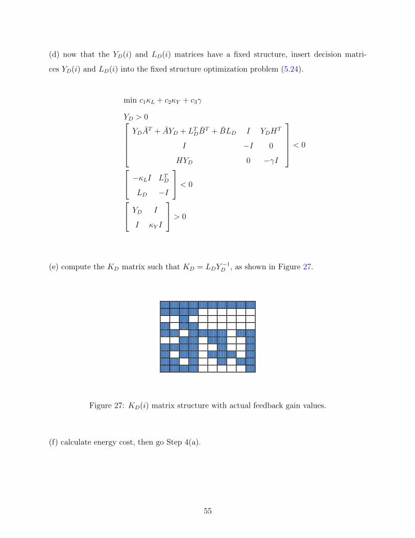
(d) now that the YD(i) and LD(i) matrices have a fixed structure, insert decision matri-
ces YD(i) and LD(i) into the fixed structure optimization problem (5.24).
min c1κL + c2κY + c3γ
YD > 0YDA
T + AYD + LTDB
T + BLD I YDHT
I −I 0
HYD 0 −γI
< 0
−κLI LTD
LD −I
< 0
YD I
I κY I
> 0
make space
(e) compute the KD matrix such that KD = LDY−1D , as shown in Figure 27. make space
Figure 27: KD(i) matrix structure with actual feedback gain values.
(f) calculate energy cost, then go Step 4(a).
make space
55
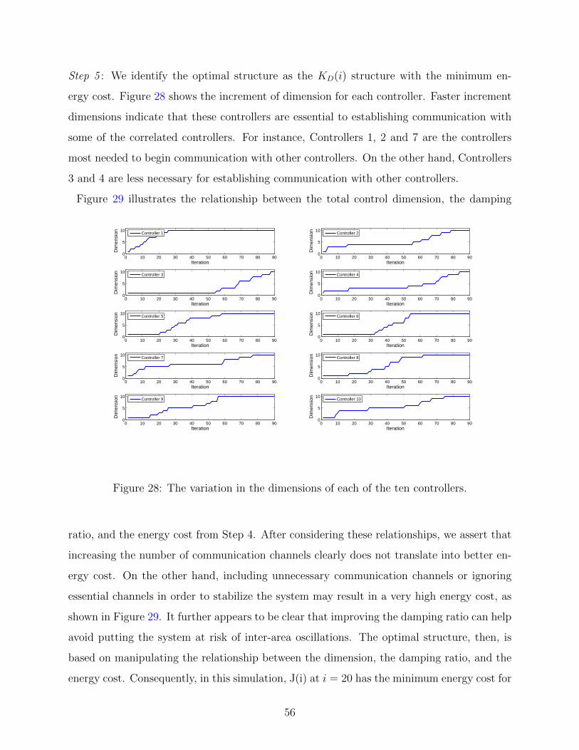
Step 5 : We identify the optimal structure as the KD(i) structure with the minimum en-
ergy cost. Figure 28 shows the increment of dimension for each controller. Faster increment
dimensions indicate that these controllers are essential to establishing communication with
some of the correlated controllers. For instance, Controllers 1, 2 and 7 are the controllers
most needed to begin communication with other controllers. On the other hand, Controllers
3 and 4 are less necessary for establishing communication with other controllers.
Figure 29 illustrates the relationship between the total control dimension, the damping
0 10 20 30 40 50 60 70 80 900
5
10
Dim
ensi
on
Iteration
Controller 1
0 10 20 30 40 50 60 70 80 900
5
10
Dim
ensi
on
Iteration
Controller 2
0 10 20 30 40 50 60 70 80 900
5
10
Dim
ensi
on
Iteration
Controller 3
0 10 20 30 40 50 60 70 80 900
5
10
Dim
ensi
onIteration
Controller 4
0 10 20 30 40 50 60 70 80 900
5
10
Dim
ensi
on
Iteration
Controller 5
0 10 20 30 40 50 60 70 80 900
5
10D
imen
sion
Iteration
Controller 6
0 10 20 30 40 50 60 70 80 900
5
10
Dim
ensi
on
Iteration
Controller 7
0 10 20 30 40 50 60 70 80 900
5
10
Dim
ensi
on
Iteration
Controller 8
0 10 20 30 40 50 60 70 80 900
5
10
Dim
ensi
on
Iteration
Controller 9
0 10 20 30 40 50 60 70 80 900
5
10
Dim
ensi
on
Iteration
Controller 10
Figure 28: The variation in the dimensions of each of the ten controllers.
ratio, and the energy cost from Step 4. After considering these relationships, we assert that
increasing the number of communication channels clearly does not translate into better en-
ergy cost. On the other hand, including unnecessary communication channels or ignoring
essential channels in order to stabilize the system may result in a very high energy cost, as
shown in Figure 29. It further appears to be clear that improving the damping ratio can help
avoid putting the system at risk of inter-area oscillations. The optimal structure, then, is
based on manipulating the relationship between the dimension, the damping ratio, and the
energy cost. Consequently, in this simulation, J(i) at i = 20 has the minimum energy cost for
56

the design of a feedback state control of this system. At the same time, the K(i) structure at
i = 20 is the optimal structure for distributed control with a high damping ratio, as shown in
Figure 30. The arrangement of the communication channels designed to connect controllers
is shown in Figure 31. Controller 1 receives state information from Controllers 3-5 and 7-10.
Controllers 1, 3, and 4 send their state variables to Controller 2. Controller 4 would receive
state information from Controllers 1 and 3 and so forth, for the other controllers.
0 10 20 30 40 50 60 70 80 900
0.2
0.4
0.6
0.8
1
Nor
mal
ized
of t
otal
dim
ensi
on c
ontr
ol
Iteration
0 10 20 30 40 50 60 70 80 900.3
0.35
0.4
0.45
0.5
0.55
Dam
ping
rat
io
Iteration
0 10 20 30 40 50 60 70 80 900.7
0.8
0.9
1
1.1
Nor
mal
ized
of c
ost (
J)
Iteration
Figure 29: The relationship between total control dimension, damping ratio, and energy
cost.
make space
57

Figure 30: Optimal feedback gain structure of distributed control.
1 2
3
4
5
6 7
8
9
10
Two-way communication
One-way communication
Figure 31: Communication channels assigned among the ten controllers.
58

6.1.4 Optimal Design Simulation
In Figure 32 we can see that all eigenvalues of the closed-loop (optimal structure) system are
on the left side of the imaginary axis of the complex plan. Therefore, the system is stable.
Furthermore, as shown in Table 6, all damping ratios corresponding to the eigenvalues are
above the critical ratio. In order to validate our design, we created non-zero initial frequency
state conditions in Areas 4 and 8, which was caused by changing of the load in these areas.
The optimal design successfully returned all states to a zero steady state after two seconds,
as shown in Figure 33. The other states in the other controller areas were not influenced by
the non-zero initial frequency state conditions. Based on the optimal structure solution, we
can write the control law for each controller, as shown in Table 7.
−20 −15 −10 −5 0−20
−15
−10
−5
0
5
10
15
20
Real
Imag
inar
y
Eigenvalues of open & closed (optimal structure) loop global systems
Open−loopClose−loop
Figure 32: Eigenvalues of open and closed (optimal structure) loop system.
59

0 0.5 1 1.5 2 2.5 3 3.5 4 4.5 5−0.2
0
0.2Frequency state response
Time (sec)
Fre
quen
cy (
p.u.
)
0 0.5 1 1.5 2 2.5 3 3.5 4 4.5 5−20
−10
0
10Power flow state response
Time (sec)
Pow
er (
p.u.
)
0 0.5 1 1.5 2 2.5 3 3.5 4 4.5 5−10
−5
0
5Mechanical power state response
Time (sec)
Pow
er (
p.u.
)
0 0.5 1 1.5 2 2.5 3 3.5 4 4.5 5−20
−10
0
10Governor power state response
Time (sec)
Pow
er (
p.u.
)
Figure 33: Control (optimal structure) system response to a non-zero initial condition in
Areas 4 and 8.
make space
60

Table 6: The eigenvalues, natural frequencies, and damping ratios for the optimal structure
Eigenvalue Frequency (Hz) Damping ratio
−0.72108 0.11476 1.00
−0.74444 0.11848 1.00
−0.8088 0.12872 1.00
−1.0575 0.16831 1.00
−4.3211 0.68773 1.00
−7.5767 1.2059 1.00
−7.847 1.2489 1.00
−22.519 3.584 1
−0.71833 ± j0.39834 0.13073 0.87453
−1.3373 ± j0.20232 0.21526 0.98875
−1.0763 ± j0.93613 0.22703 0.75454
−1.5512 ± j0.29733 0.25137 0.98212
−1.8488 ± j0.399 0.30102 0.97749
−1.9307 ± j0.70375 0.32706 0.93953
−5.2834 ± j5.3005 1.1911 0.70597
−4.5556 ± j8.1267 1.4828 0.48898
−4.9626 ± j8.9686 1.6313 0.48415
−7.0743 ± j7.4667 1.6370 0.68777
−7.0626 ± j8.0457 1.7039 0.6597
−7.8056 ± j8.0436 1.7839 0.69641
−7.1454 ± j8.8194 1.8065 0.62951
−7.5779 ± j8.7012 1.8364 0.65675
−8.3967 ± j11.02 2.2050 0.60608
−8.9823 ± j12.007 2.3865 0.59903
61

Table 7: Control laws for the ten controllers.
Area Note
u1(t) = K1X1(t) K1 = [K11, K13, K14, K15, K17, K18, K19, K110] and
X1(t) =[x1(t);x
d3(t);x
d4(t);x
d5(t);x
d7(t);x
d8(t);
xd9(t);xd10(t)
]u2(t) = K2X2(t) K2 = [K21, K22, K23, K24] and
X2(t) =[xd1(t);x2(t);x
d3(t), x
d4(t)]
u3(t) = K3X3(t) K3 = [K33] and X3 = [x3(t)]
u4(t) = K4X4(t) K4 = [K41, K43, K44] and
X4(t) =[xd1(t);x
d3(t);x4(t)
]u5(t) = K5X5(t) K5 = [K55] and X5(t) = [x5(t)]
u6(t) = K6X6(t) K6 = [K66] and X6(t) = [x6(t)]
u7(t) = K7X7(t) K7 = [K72, K73, K74, K77, K710] and
X7(t) =[xd2(t);x
d3(t);x
d4(t);x7(t);x
d10(t)
]u8(t) = K8X8(t) K8 = [K83, K88] and X8(t) =
[xd3(t);x8(t)
]u9(t) = K9X9(t) K9 = [K94, K99, K910] and
X9(t) =[xd4(t);x9(t);x
d10(t)
]u10(t) = K10X10(t) K10 = [K102, K103, K104, K1010] and
X10(t) =[xd2(t);x
d3(t);x
d4(t);x10(t)
]where Kii and xi are the gain matrix and state vector for local controller i,
respectively. Kij is the gain matrix assigned to the state information (xdj )
which is sent from node j.
62

6.2 DISCUSSION
The main purpose of this section is to compare the performance of our optimal structure
with those of random fixed structures, a completely decentralized structure, and a centralized
structure. For the purpose of this comparison, the fixed structures were randomly chosen,
as shown in Figure 34, with the exception the ”Y” structure, for which we allowed the
same areas to be connected through tie-lines, enabling additional communication, as shown
previously in Figure 18. Each small square represents a subsystem (area). For example in
the ”Y” structure, Subsystem 1 sends local state variables to Subsystems 2,3, and 4, and
receives their state variables. We applied the same paradigm to all other subsystems. Figure
35 shows the dimensions of each single controller in the control structure.
(a) Comp. decentralized structure
(b) "X" structure
(c) "Y" structure
(d) "Z" structure
(e) Optimal structure
(f) Centralized structure
Figure 34: Various control structures.
make space
63

0
1
2
3
4
5
6
7
8
9
10
Decentralized "Z" "Y" "X" Optimal Centralized
C1 C2 C3 C4 C5 C6 C7 C8 C9 C10
Figure 35: Controllers dimensions for all control structures.
Figures 38, 39, 40, 41, and 42 illustrate that the feedback control designed for all struc-
tures were able to stabilize the system by returning the disturbance states to zero steady
state when non-zero initial frequency conditions were created in Areas 4 and 8. However,
there are significant differences between these control structures. Figure 36 clearly supports
the conclusion that the central controller represents significant additional damping of the
system. Figure 29 shows a comparison between the control dimension and energy cost. The
centralized structure has the lowest energy cost, but it has a full dimensional controller. On
the other hand, the completely decentralized structure has the lowest controller dimension
but entails high energy cost. When we moved from a completely decentralized structure
to the ”Z” structure by allowing some controllers to communicate, the energy cost is still
high. By allowing more controllers to communicate as in the ”Y” structure, we still were not
64

successful at decreasing the energy cost. This finding would indicate that adding unneces-
sary communication between controllers does not improve performance. Moving to the ”X”
structure by assigning more than half of the available communication channels improved
the performance, but still did not guarantee getting the minimum energy cost. However,
our model was able to obtain the best structure between controllers in order to meet power
system stabilization requirements at minimum energy cost.
0
0.1
0.2
0.3
0.4
0.5
0.6
0.7
Decentralized "Z" "Y" "X" Optimal Centralized
Figure 36: Lowest five damping ratios.
make space
65

0
0.2
0.4
0.6
0.8
1
Decentralized "Z" "Y" "X" Optimal Centralized
Total cost (J) Dimension control
Figure 37: Total control dimension vs. energy cost for different control structures.
66

0 0.5 1 1.5 2 2.5 3 3.5 4 4.5 5−0.2
−0.1
0
Frequency state response
Time (sec)
Fre
quen
cy (
p.u.
)
0 0.5 1 1.5 2 2.5 3 3.5 4 4.5 5−10
−5
0
Power flow state response
Time (sec)
Pow
er (
p.u.
)
0 0.5 1 1.5 2 2.5 3 3.5 4 4.5 5−10
−5
0
Mechanical power state response
Time (sec)
Pow
er (
p.u.
)
0 0.5 1 1.5 2 2.5 3 3.5 4 4.5 5−20
−10
0
Governor power state response
Time (sec)
Pow
er (
p.u.
)
Figure 38: Control (completely decentralized structure) system response to a non-zero initial
condition in Areas 4 and 8.
0 0.5 1 1.5 2 2.5 3 3.5 4 4.5 5−0.2
−0.1
0
Frequency state response
Time (sec)
Fre
quen
cy (
p.u.
)
0 0.5 1 1.5 2 2.5 3 3.5 4 4.5 5−10
−5
0
Power flow state response
Time (sec)
Pow
er (
p.u.
)
0 0.5 1 1.5 2 2.5 3 3.5 4 4.5 5−10
−5
0
Mechanical power state response
Time (sec)
Pow
er (
p.u.
)
0 0.5 1 1.5 2 2.5 3 3.5 4 4.5 5−20
−10
0
Governor power state response
Time (sec)
Pow
er (
p.u.
)
Figure 39: Control (”X” structure) system response to a non-zero initial condition in Areas
4 and 8.
67

0 0.5 1 1.5 2 2.5 3 3.5 4 4.5 5−0.2
−0.1
0
Frequency state response
Time (sec)
Fre
quen
cy (
p.u.
)
0 0.5 1 1.5 2 2.5 3 3.5 4 4.5 5−10
−5
0
Power flow state response
Time (sec)
Pow
er (
p.u.
)
0 0.5 1 1.5 2 2.5 3 3.5 4 4.5 5−10
−5
0
Mechanical power state response
Time (sec)
Pow
er (
p.u.
)
0 0.5 1 1.5 2 2.5 3 3.5 4 4.5 5−20
−10
0
Governor power state response
Time (sec)
Pow
er (
p.u.
)
Figure 40: Control (”Y” structure) system response to a non-zero initial condition in Areas
4 and 8..
0 0.5 1 1.5 2 2.5 3 3.5 4 4.5 5−0.2
−0.1
0
Frequency state response
Time (sec)
Fre
quen
cy (
p.u.
)
0 0.5 1 1.5 2 2.5 3 3.5 4 4.5 5−10
−5
0
Power flow state response
Time (sec)
Pow
er (
p.u.
)
0 0.5 1 1.5 2 2.5 3 3.5 4 4.5 5−10
−5
0
Mechanical power state response
Time (sec)
Pow
er (
p.u.
)
0 0.5 1 1.5 2 2.5 3 3.5 4 4.5 5−20
−10
0
Governor power state response
Time (sec)
Pow
er (
p.u.
)
Figure 41: Control (”Z” structure) system response to a non-zero initial condition in Areas
4 and 8.
68

0 0.5 1 1.5 2 2.5 3 3.5 4 4.5 5−0.2
0
0.2Frequency state response
Time (sec)
Fre
quen
cy (
p.u.
)
0 0.5 1 1.5 2 2.5 3 3.5 4 4.5 5−10
−5
0
Power flow state response
Time (sec)
Pow
er (
p.u.
)
0 0.5 1 1.5 2 2.5 3 3.5 4 4.5 5−4
−2
0
2Mechanical power state response
Time (sec)
Pow
er (
p.u.
)
0 0.5 1 1.5 2 2.5 3 3.5 4 4.5 5−15
−10
−5
0
5Governor power state response
Time (sec)
Pow
er (
p.u.
)
Figure 42: Control (centralized structure) system response to a non-zero initial condition in
Areas 4 and 8.
69

7.0 CONCLUSION
Dimensionality reduction in a controller structure produces effective control signals with
reduced computational load. In the control design of large-scale power systems, the ma-
nipulation of effective control signals, diminutive control dimensions, and suitable damping
ratios presents a very challenging problem. The model we demonstrate in his thesis pro-
vides a solution to this challenge by integrating control and communication in the design of
advance control structures for large-scale power systems. In particular, the control system
present here avoids the potential ineffective performance of system based on fixed structures,
which either include unnecessary communication channels or exclude essential communica-
tion channels between controllers. In our simulation, we have shown that the relationship
between the control signal and the control dimension is based on system behavior. We were
able to reduce the communication complexity of the control design and design a communi-
cation structure in order to achieve robust control.
Unlike other studies, in which the communication was indirectly reflected by a topology
dependent matrix in the LQR cost function, our model considers the control structure and its
communication channels in the cost function which helps to punish communication complex-
ity of the controller structure. As a result our model was able to recognize communications
as either essential or unessential during the design of the controller structure and thereby
reduce the dimension of the controller. A design for distributed control, which is essential to
suppressing inter-area low frequency oscillations in large-scale power systems, was presented
in this thesis.
In the designing centralized or distributed control structures, communication constraints
and time delay should be taken into account, in order to satisfy the performance specifications
of a large-scale power system. Recent studies ignore the impact of time delay on the design
70

of robust control. If communication constraints and time delay are not considered in the
design of such distributed control, system performance may be weak and may even cause
instability in the system.
The design presented in this thesis creates innovative schemes for the system control
design of a power system and is expected to contribute significantly to the national needs for
power system control. First, this study integrates control and communication in the design
of advanced control architectures for complex and large scale engineering systems, including
the power system in this country and internationally. The principles, methods, and tools
developed from this study enables the building of more complex systems and will ensure that
these systems are reliable, efficient, and robust. Second, this study offers more applications
in the field of power system control. The detailed implementation of the hierarchical control
in this study can serve as a guideline, which can be readily generalized to other optimization
and control problems in power systems, such as the optimal power flow problem [9] and the
dynamic unit commitment problem [85]. Third, this study of control in complex networks
will accelerate the progress of other research areas in complex networked systems, such as
understanding network structure, understanding network dynamics, and predictive modeling
and simulation for networks [20].
71

APPENDIX
MORE SIMULATION RESULTS
−20 −15 −10 −5 0−20
−15
−10
−5
0
5
10
15
20
Real
Imag
inar
y
Eigenvalues of open & closed (completely decentralized structure) loop global systems
Open−loopClose−loop
Figure 43: Eigenvalues of the closed-loop (decentralized structure) system.
72

−20 −15 −10 −5 0−20
−15
−10
−5
0
5
10
15
20
Real
Imag
inar
y
Eigenvalues of open & closed ("X" structure) loop global systems
Open−loopClose−loop
Figure 44: eigenvalues of the closed-loop (”X” structure) system.
73

−20 −15 −10 −5 0−20
−15
−10
−5
0
5
10
15
20
Real
Imag
inar
y
Eigenvalues of open & closed ("Y" structure) loop global systems
Open−loopClose−loop
Figure 45: eigenvalues of the closed-loop (”Y” structure) system.
74

−20 −15 −10 −5 0−20
−15
−10
−5
0
5
10
15
20
Real
Imag
inar
y
Eigenvalues of open & closed ("Z" structure) loop global systems
Open−loopClose−loop
Figure 46: Eigenvalues of the closed-loop (”Z” structure) system.
75

−20 −15 −10 −5 0−20
−15
−10
−5
0
5
10
15
20
Real
Imag
inar
y
Eigenvalues of open & closed (centralized structure) loop global systems
Open−loopClose−loop
Figure 47: Eigenvalues of the closed-loop (centralized structure) system.
76

Table 8: The eigenvalues, natural frequencies, and damping ratios for the centralized struc-
ture.
Eigenvalue Frequency (Hz) Damping ratio
−0.69316 0.11032 1
−1.5874 0.25265 1
−2.5062 0.39887 1
−2.8874 0.45955 1
− 4.7005 0.74811 1
−8.1858 1.3028 1
−8.647 1.3762 1
− 12.264 1.9518 1
−3.2465 ± j1.4159 0.5637 0.9166
−1.6037 ± j0.36607 0.2618 0.9749
−2.2552 ± j0.3967 0.36444 0.9848
−1.8788 ± j 4.4925 0.77501 0.3858
−2.1211 ± j 4.9558 0.85794 0.3934
−2.324 ± j6.1393 1.0448 0.3540
−7.428 ± j0.16033 1.1825 0.9997
−3.4794 ± j 7.6899 1.3433 0.4122
−1.7802 ± j8.6778 1.4099 0.2009
−0.72728 ± j 9.9041 1.5805 0.0732
−2.3382 ± j 9.7529 1.5962 0.2331
−7.8041 ± j 8.1038 1.7906 0.6936
−3.1033 ± j 11.116 1.8368 0.2689
−5.9278 ± j 10.585 1.9308 0.4886
−12.658 ± j4.7356 2.1510 0.9366
− 5.8564 ± j 14.168 2.4400 0.3820
77

Table 9: The eigenvalues, natural frequencies, and damping ratios for the completely decen-
tralized structure.
Eigenvalue Frequency (Hz) Damping ratio
−0.69428 0.1105 1
−0.72404 0.11523 1
−0.75599 0.12032 1
−1.0571 0.16824 1
−4.3295 0.68906 1
−5.9268 0.94327 1
−7.2437 1.1529 1
−7.6724 1.2211 1
−0.71666 ± j 0.40385 0.13092 0.8712
−0.95019 ± j0.62198 0.18075 0.8366
−0.93525 ± j0.82541 0.19853 0.7497
−1.4052 ± j0.36455 0.23104 0.9679
−1.6828 ± j0.45002 0.27725 0.9660
−1.6931 ± j 0.50219 0.28107 0.9587
−5.283 ± j5.3029 1.1913 0.7057
−4.3205 ± j7.9709 1.443 0.4765
−5.082 ± j8.4639 1.5712 0.5147
−7.1256 ± j 7.4649 1.6425 0.6904
−7.139 ± j8.0028 1.7068 0.6656
−7.8202 ± j8.0183 1.7826 0.6982
−7.1796 ± j8.6827 1.7931 0.6372
−7.8532 ± j 8.771 1.8737 0.6670
−8.4416 ± j 10.972 2.2033 0.6097
−8.9831 ± j12.007 2.3865 0.5990
78

Table 10: The eigenvalues, natural frequencies, and damping ratios for open-loop system.
Eigenvalue Frequency (Hz) Damping ratio
−1.2391 0.1972 1
−1.5548 0.2476 1
−2.3351 0.37163 1
−2.5308 0.40279 1
−2.656 0.42272 1
−2.9548 0.47027 1
−3.0597 0.48696 1
−3.3167 0.52787 1
−5.5592 0.88477 1
−5.9535 0.94753 1
−6.0219 0.95842 1
−6.2948 1.0019 1
−6.344 1.0097 1
−6.6197 1.0536 1
−6.8357 1.0879 1
−7.0185 1.117 1
−7.6245 1.2135 1
−7.9511 1.2655 1
3.6457e-16 5.8023e-17 -1
0.81081 ± j 4.0553 0.65819 −0.19606
1.383 ± j 5.7033 0.93401 −0.23566
1.2899 ± j 7.0433 1.1396 −0.18015
1.6634 ± j 7.4759 1.2189 −0.21719
1.5923 ± j 9.4434 1.5242 −0.16627
79

Table 11: The eigenvalues, natural frequencies, and damping ratios for open-loop system
(cont.).
Eigenvalue Frequency (Hz) Damping ratio
1.7368 ± j 10.225 1.6507 −0.16746
1.6581 ± j 11.522 1.8527 −0.14244
1.6974 ± j 13.516 2.1681 −0.12461
1.7646 ± j 15.728 2.5189 −0.1115
1.9111 ± j 17.801 2.8494 −0.10674
80
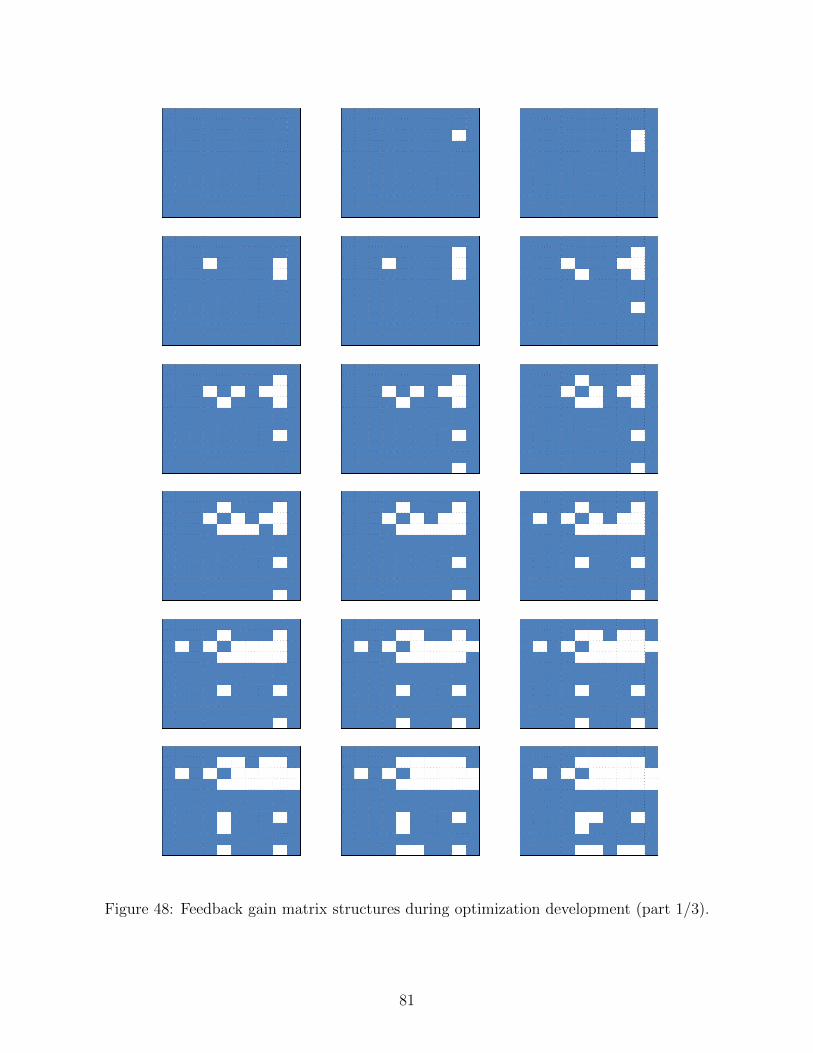
Figure 48: Feedback gain matrix structures during optimization development (part 1/3).
81

Figure 49: Feedback gain matrix structures during optimization development (part 2/3).
82

Figure 50: Feedback gain matrix structures during optimization development (part 3/3).
83

BIBLIOGRAPHY
[1] The Earth Observatory is part of the EOS Project Science Office located at NASA God-dard Space Flight Center.
[2] U.S. National Grid Map. Global Energy Network Institute.
[3] U S Energy Information Administration. Annual Energy Outlook 2012, with ProjectionsTo 2035. U.S. Government Printing Office, 2012.
[4] U S Energy Information Administration. Early Release Overview of Annual EnergyOutlook 2013, with Projections To 2040. U.S. Government Printing Office, 2013.
[5] L.A. Aguirre. Quantitative measure of modal dominance for continuous systems. InDecision and Control, 1993., Proceedings of the 32nd IEEE Conference on, pages 2405–2410 vol.3, dec 1993.
[6] B.D.O. Anderson and A.C. Antoulas. Rational interpolation and state variable real-izations. In Decision and Control, 1990., Proceedings of the 29th IEEE Conference on,pages 1865 –1870 vol.3, dec 1990.
[7] A. C. Antoulas, D. C. Sorensen, and S. Gugercin. A survey of model reduction methodsfor large-scale systems. Contemporary Mathematics, 280:193–219, 2001.
[8] P. Antsaklis and J. Baillieul. Special issue on technology of networked control systems.Proceedings of the IEEE, 95(1):5 –8, jan. 2007.
[9] A.M. Azmy. Optimal power flow to manage voltage profiles in interconnected networksusing expert systems. Power Systems, IEEE Transactions on, 22(4):1622 –1628, nov.2007.
[10] W. Bajwa, J. Haupt, A. Sayeed, and R. Nowak. Joint source-channel communicationfor distributed estimation in sensor networks. Information Theory, IEEE Transactionson, 53(10):3629 –3653, oct. 2007.
[11] G.A. Baker. Essentials of Pade approximants. Academic Press, 1975.
84

[12] Mikhail Belkin and Partha Niyogi. Laplacian eigenmaps and spectral techniques forembedding and clustering. In Advances in Neural Information Processing Systems 14,pages 585–591. MIT Press, 2001.
[13] Wang Bo, Quanyuan Jiang, and Yijia Cao. Transmission network fault location us-ing sparse pmu measurements. In Sustainable Power Generation and Supply, 2009.SUPERGEN ’09. International Conference on, pages 1 –6, april 2009.
[14] K. Bollinger and R. Lalonde. Tuning synchronous generator voltage regulators using on-line generator models. Power Apparatus and Systems, IEEE Transactions on, 96(1):32–37, Jan.
[15] K.E. Bollinger, R. Winsor, and A. Campbell. Frequency response methods for tuningstabilizers to damp out tie-line power oscillations: Theory and field-test results. PowerApparatus and Systems, IEEE Transactions on, PAS-98(5):1509–1515, Sept.
[16] D. BONVIN and D. A. MELLICHAMP. A unified derivation and critical review ofmodal approaches to model reduction. International Journal of Control, 35(5):829–848,1982.
[17] S. Boyd, L. El Ghaoui, E. Feron, and V. Balakrishnan. Linear Matrix Inequalitiesin System and Control Theory, volume 15 of Studies in Applied Mathematics. SIAM,Philadelphia, PA, June 1994.
[18] S. Boyd, L.E. Ghaoul, E. Feron, and V. Balakrishnan. Linear Matrix Inequalities inSystem and Control Theory. Siam Studies in Applied Mathematics. Society for Industrialand Applied Mathematics, 1994.
[19] Matthew Brand. Charting a manifold. In Advances in Neural Information ProcessingSystems 15, pages 961–968. MIT Press, 2003.
[20] James M. Brase and David L. Brown. Modeling, simulation and analysis ofcomplexnetworked systems: A program plan. 2009.
[21] Dennis J. Brueni and Lenwood S. Heath. The pmu placement problem. SIAM J. Discret.Math., 19(3):744–761, July 2005.
[22] E.J. Candes, J. Romberg, and T. Tao. Robust uncertainty principles: exact signal re-construction from highly incomplete frequency information. Information Theory, IEEETransactions on, 52(2):489 – 509, feb. 2006.
[23] E.J. Candes and M.B. Wakin. An introduction to compressive sampling. Signal Pro-cessing Magazine, IEEE, 25(2):21 –30, march 2008.
[24] D. Chaniotis and M.A. Pai. Model reduction in power systems using krylov subspacemethods. Power Systems, IEEE Transactions on, 20(2):888 – 894, may 2005.
85

[25] N.R. Chaudhuri, B. Chaudhuri, S. Ray, and R. Majumder. Wide-area phasor poweroscillation damping controller: A new approach to handling time-varying signal latency.Generation, Transmission Distribution, IET, 4(5):620–630, May.
[26] C.T. Chen. Linear System Theory and Design. The Oxford Series In Electrical AndComputer Engineering. Oxford University Press, 1999.
[27] J.H. Chow, Juan J. Sanchez-Gasca, Haoxing Ren, and S. Wang. Power system dampingcontroller design-using multiple input signals. Control Systems, IEEE, 20(4):82–90, Aug.
[28] T.F. Cox and M.A.A. Cox. Multidimensional Scaling. Monographs on Statistics andApplied Probability. Chapman & Hall/CRC, 2001.
[29] M. L. Crow, C. Gill, F. Liu, B. Mcmillin, D. Niehaus, and D. Tauritz. Engineeringthe advanced power grid: Research challenges and tasks. In RTAS 2006 Workshop onResearch Directions for Security and Networking in Critical Real-Time and EmbeddedSystems, 2006.
[30] Vasudev Gharpure Damir Novosel Daniel Karlsson Mehmet Kaba David G. Hart,David Uy. Pmus a new approach to power network monitoring. ABB Review, pages58–61, 2001.
[31] F.P. DeMello and Charles Concordia. Concepts of synchronous machine stability asaffected by excitation control. Power Apparatus and Systems, IEEE Transactions on,PAS-88(4):316–329, April.
[32] David L. Donoho and Michael Elad. Optimally sparse representation in general (non-orthogonal) dictionaries via 1 minimization. In Proc. Natl Acad. Sci. USA 100 2197202,2003.
[33] D.L. Donoho. Compressed sensing. Information Theory, IEEE Transactions on,52(4):1289 –1306, april 2006.
[34] D. Dotta, A.S. e Silva, and I.C. Decker. Wide-area measurements-based two-level controldesign considering signal transmission delay. Power Systems, IEEE Transactions on,24(1):208 –216, feb. 2009.
[35] H.G. Far, H. Banakar, Pei Li, Changling Luo, and Boon-Teck Ooi. Damping interareaoscillations by multiple modal selectivity method. Power Systems, IEEE Transactionson, 24(2):766–775, May.
[36] P. Gahinet, A. Nemirovski, A. J. Laub, and M. Chilali. LMI Control Toolbox: For usewith MATLAB. 1995.
[37] A.J. Germond and R. Podmore. Dynamic aggregation of generating unit models. PowerApparatus and Systems, IEEE Transactions on, PAS-97(4):1060–1069, July.
86

[38] J.C. Geromel, J. Bernussou, and P.L.D. Peres. Decentralized control through parameterspace optimization. Automatica, 30(10):1565 – 1578, 1994.
[39] G.H. Golub and C.F. Van Loan. Matrix Computations. Johns Hopkins Studies in theMathematical Sciences. Johns Hopkins University Press, 1996.
[40] B. Gou. Generalized integer linear programming formulation for optimal pmu placement.Power Systems, IEEE Transactions on, 23(3):1099 –1104, aug. 2008.
[41] J. Haupt, W.U. Bajwa, M. Rabbat, and R. Nowak. Compressed sensing for networkeddata. Signal Processing Magazine, IEEE, 25(2):92 –101, march 2008.
[42] S. Haykin and E. Moulines. Special issue on large-scale dynamic systems. Proceedingsof the IEEE, 95(5):849 –852, may 2007.
[43] Bruce A. Hendrickson and Margaret H. Wright. Mathematical research challenges inoptimization of complex systems. 2006.
[44] S. Hirano, T. Michigami, A. Kurita, D.B. Klapper, N.W. Miller, J.J. Sanchez-Gasca, andT.D. Younkins. Functional design for a system-wide multivariable damping controller[for power systems]. Power Systems, IEEE Transactions on, 5(4):1127–1136, Nov.
[45] D.D. iljak and A.I. Zeevi. Control of large-scale systems: Beyond decentralized feedback.Annual Reviews in Control, 29(2):169 – 179, 2005.
[46] The NETL Modern Grid Initiative. A systems view of the modern grid. 2007.
[47] A. Ishchenko, J.M.A. Myrzik, and W.L. Kling. Dynamic equivalencing of distributionnetworks with dispersed generation using hankel norm approximation. Generation,Transmission Distribution, IET, 1(5):818 –825, september 2007.
[48] M. Jamshidi. Large-scale systems: modeling, control, and fuzzy logic. Prentice Hallseries on environmental and intelligent manufacturing systems. Prentice Hall, 1997.
[49] I.T. Jolliffe. Principal Component Analysis. Springer Series in Statistics. Springer-Verlag, 2002.
[50] I. Kamwa, R. Grondin, D. Asber, J.P. Gingras, and G. Trudel. Active-power stabiliz-ers for multimachine power systems: challenges and prospects. Power Systems, IEEETransactions on, 13(4):1352–1358, Nov.
[51] I. Kamwa, R. Grondin, and Y. Hebert. Wide-area measurement based stabilizing controlof large power systems-a decentralized/hierarchical approach. Power Systems, IEEETransactions on, 16(1):136–153, Feb.
[52] P.C. Krause and J.N. Towle. Synchronous machine damping by excitation control withdirect and quadrature axis field windings. Power Apparatus and Systems, IEEE Trans-actions on, PAS-88(8):1266–1274, Aug.
87

[53] P. Kundur, N.J. Balu, and M.G. Lauby. Power system stability and control. The EPRIpower system engineering series. McGraw-Hill, 1994.
[54] P. Kundur, M. Klein, G.J. Rogers, and M.S. Zywno. Application of power system sta-bilizers for enhancement of overall system stability. Power Systems, IEEE Transactionson, 4(2):614–626, May.
[55] Cedric Langbort and Vijay Gupta. Minimal interconnection topology in distributedcontrol design. SIAM J. Control Optim., 48(1):397–413, February 2009.
[56] E.V. Larsen and D. A. Swann. Applying power system stabilizers part i: Generalconcepts. Power Apparatus and Systems, IEEE Transactions on, PAS-100(6):3017–3024, June.
[57] E.V. Larsen and D. A. Swann. Applying power system stabilizers part ii: Performanceobjectives and tuning concepts. Power Apparatus and Systems, IEEE Transactions on,PAS-100(6):3025–3033, June.
[58] E.V. Larsen and D. A. Swann. Applying power system stabilizers part iii: Practical con-siderations. Power Apparatus and Systems, IEEE Transactions on, PAS-100(6):3034–3046, June.
[59] M.H.C. Law and A.K. Jain. Incremental nonlinear dimensionality reduction by manifoldlearning. Pattern Analysis and Machine Intelligence, IEEE Transactions on, 28(3):377–391, march 2006.
[60] J. Lfberg. Yalmip : A toolbox for modeling and optimization in MATLAB. In Proceed-ings of the CACSD Conference, Taipei, Taiwan, 2004.
[61] Chao Lu, Jennie Si, Xiaochen Wu, and Peng Li. Approximate dynamic programmingcoordinated control in multi-infeed hvdc power system. In Power Systems Conferenceand Exposition, 2006. PSCE ’06. 2006 IEEE PES, pages 2131 –2135, 29 2006-nov. 12006.
[62] J. Machowski, J. Bialek, and J.R. Bumby. Power system dynamics and stability. JohnWiley, 1997.
[63] N. Martins, L.T.G. Lima, and H.J.C.P. Pinto. Computing dominant poles of powersystem transfer functions. Power Systems, IEEE Transactions on, 11(1):162 –170, feb1996.
[64] S. Mohagheghi, G.K. Venayagamoorthy, and R.G. Harley. Optimal wide area con-troller and state predictor for a power system. Power Systems, IEEE Transactions on,22(2):693–705, May.
[65] J.A. Momoh. Smart grid design for efficient and flexible power networks operation andcontrol. In Power Systems Conference and Exposition, 2009. PSCE ’09. IEEE/PES,pages 1 –8, march 2009.
88

[66] B. Moore. Principal component analysis in linear systems: Controllability, observability,and model reduction. Automatic Control, IEEE Transactions on, 26(1):17 – 32, feb 1981.
[67] Y. Nesterov and A. Nemirovskii. Interior Point Polynomial Algorithms in Convex Pro-gramming. Studies in Applied and Numerical Mathematics. Society for Industrial andApplied Mathematics, 1987.
[68] Hui Ni, G.T. Heydt, and L. Mili. Power system stability agents using robust wide areacontrol. Power Systems, IEEE Transactions on, 17(4):1123 – 1131, nov 2002.
[69] F. Okou, L-A Dessaint, and O. Akhrif. Power systems stability enhancement using awide-area signals based hierarchical controller. Power Systems, IEEE Transactions on,20(3):1465–1477, Aug.
[70] International Conference on Large High Voltage Electric Systems. Analysis and Controlof Power System Oscillations: Final Report. CIGRE technical brochure. CIGRE, 1996.
[71] B. Pal and B. Chaudhuri. Robust Control in Power Systems. Power Electronics andPower Systems. Springer, 2005.
[72] B. Pal and B. Chaudhuri. Robust Control in Power Systems. Power Electronics AndPower Systems. Springer, 2005.
[73] F. Palacios-Quinonero and J. M. Rossell. Decentralized control with information struc-ture constraints. 15th International Workshop on Dynamics and Control, 2009.
[74] Wei Qiao, Ganesh K. Venayagamoorthy, and Ronald G. Harley. Optimal wide-areamonitoring and nonlinear adaptive coordinating neurocontrol of a power system withwind power integration and multiple facts devices. Neural Networks, 21(23):466 – 475,2008.
[75] Chawasak Rakpenthai, Suttichai Premrudeepreechacharn, Sermsak Uatrongjit, andNeville R. Watson. An optimal pmu placement method against measurement loss andbranch outage. Power Delivery, IEEE Transactions on, 22(1):101 –107, jan. 2007.
[76] Sara Robinson. The Power Grid: Fertile Ground for Math Research. SIAM News, 2003.
[77] G. Rogers. Power system oscillations. Kluwer international series in engineering andcomputer science: Power electronics & power systems. Kluwer Academic, 2000.
[78] G. Rogers. Power system oscillations. Kluwer international series in engineering andcomputer science: Power electronics & power systems. Kluwer Academic, 2000.
[79] G. Rogers. Demystifying power system oscillations. Computer Applications in Power,IEEE, 9(3):30–35, Jul.
[80] Sam T. Roweis and Lawrence K. Saul. Nonlinear dimensionality reduction by locallylinear embedding. Science, 290(5500):2323–2326, 2000.
89

[81] Jr. Sandell, N. and M. Athans. Solution of some nonclassical lqg stochastic decisionproblems. Automatic Control, IEEE Transactions on, 19(2):108 – 116, apr 1974.
[82] Jr. Sandell, N., P. Varaiya, M. Athans, and M. Safonov. Survey of decentralized controlmethods for large scale systems. Automatic Control, IEEE Transactions on, 23(2):108– 128, apr 1978.
[83] J. Shawe-Taylor and N. Cristianini. Kernel Methods for Pattern Analysis. CambridgeUniversity Press, 2004.
[84] D.D. Siljak. Large-Scale Dynamic Systems: Stability and Structure. Dover Civil andMechanical Engineering Series. Dover Publications, 2007.
[85] T.K. Siu, G.A. Nash, and Z.K. Shawwash. A practical hydro dynamic unit commitmentand loading model. In Power Industry Computer Applications, 2001. PICA 2001. In-novative Computing for Power - Electric Energy Meets the Market. 22nd IEEE PowerEngineering Society International Conference on, pages 26 –29, 2001.
[86] J. F. Sturm. Using sedumi 1.02, a MATLAB toolbox for optimization over symmetriccones. Optimization Methods and Software, 11–12:625–653, 1999.
[87] Joshua B. Tenenbaum, Vin de Silva, and John C. Langford. A global geometric frame-work for nonlinear dimensionality reduction. Science, 290(5500):2319–2323, 2000.
[88] Li Teng, Hongyu Li, Xuping Fu, Wenbin Chen, and I-Fan Shen. Dimension reductionof microarray data based on local tangent space alignment. In Cognitive Informatics,2005. (ICCI 2005). Fourth IEEE Conference on, pages 154 – 159, aug. 2005.
[89] T. Van Cutsem and C. Vournas. Voltage Stability of Electric Power Systems. KluwerInternational Series in Engineering and Computer Science. Kluwer Academic Publishers,1998.
[90] R. Witzmann. Damping of interarea oscillations in large interconnected power systems.IPST 2001, pages 411–416, 2001.
[91] Hansheng Wu. Decentralized adaptive robust control for a class of large-scale systemsincluding delayed state perturbations in the interconnections. Automatic Control, IEEETransactions on, 47(10):1745 – 1751, oct 2002.
[92] Hongxia Wu, K.S. Tsakalis, and G.T. Heydt. Evaluation of time delay effects to wide-area power system stabilizer design. Power Systems, IEEE Transactions on, 19(4):1935–1941, Nov.
[93] A.I. Zecevic and D.D. Siljak. Control Of Complex Systems: Structural Constraints andUncertainty. Communications and Control Engineering. Springer, 2010.
[94] A.I. Zeevi and D.D. iljak. Control design with arbitrary information structure con-straints. Automatica, 44(10):2642 – 2647, 2008.
90

[95] Yang Zhang and A. Bose. Design of wide-area damping controllers for interarea oscilla-tions. Power Systems, IEEE Transactions on, 23(3):1136–1143, Aug.
[96] M. Zima, M. Larsson, P. Korba, C. Rehtanz, and G. Andersson. Design aspects forwide-area monitoring and control systems. Proceedings of the IEEE, 93(5):980–996,May.
[97] R.D. Zimmerman, C.E. Murillo-Sanchez, and R.J. Thomas. Matpower: Steady-state op-erations, planning, and analysis tools for power systems research and education. PowerSystems, IEEE Transactions on, 26(1):12 –19, feb. 2011.
91