Accident Analysis and Prevention xxx (2003) xxx–xxx

An accident waiting to happen: a spatial approach toproactive pedestrian planning

Robert J. Schneider∗, Rhonda M. Ryznar1, Asad J. Khattak1

Department of City and Regional Planning, University of North Carolina at Chapel Hill, CB 3140 New East Bldg., Chapel Hill, NC 27599-3140, USA

Received 14 May 2001; received in revised form 21 January 2002; accepted 13 February 2002

Abstract

There are about 75,000 pedestrian crashes in the United States each year. Approximately 5000 of these crashes are fatal, accounting for12% of all roadway deaths. On college campuses, pedestrian exposure and crash-risk can be quite high. Therefore, we analyzed pedestriancrashes on the campus of the University of North Carolina at Chapel Hill (UNC) as a test case for our spatially-oriented prototype toolthat combines perceived-risk (survey) data with police-reported crash data to obtain a more complete picture of pedestrian crash-risk. Weuse spatial analysis techniques combined with regression models to understand factors associated with risk. The spatial analysis is basedon comparing two distributions, i.e. the locations of perceived-risk with police-reported crash locations. The differences between the twodistributions are statistically significant, implying that certain locations on campus are perceived as dangerous, though pedestrian crasheshave not yet occurred there, and there are actual locations of police-reported crashes that are not perceived to be dangerous by pedestriansor drivers. Furthermore, we estimate negative binomial regression models to combine pedestrian and automobile exposure with roadwaycharacteristics and spatial/land use information. The models show that high exposure, incomplete sidewalks and high crosswalk densityare associated with greater observed and perceived pedestrian crash-risk. Additionally, we found that people perceive a lower risk nearuniversity libraries, stadiums, and academic buildings, despite the occurrence of crashes.© 2003 Elsevier Science Ltd. All rights reserved.

Keywords:Pedestrian; Safety; Survey; Spatial Analysis; Geographic Information Systems; Negative binomial model

1. Introduction

On average, a pedestrian injury occurs every 6 min anda pedestrian fatality occurs every 107 min in the UnitedStates (NHTSA, 2000). The 4906 pedestrian fatalities in1999 accounted for approximately 12% of highway deathsthat year (BTS, 1999). Yet, this fact may inspire little localaction until a serious pedestrian injury or fatality occurs ina neighborhood, in a specific commercial area, or on a col-lege campus. One of the 4906 pedestrian fatalities of 1999occurred in November on the campus of the University ofNorth Carolina at Chapel Hill (UNC) when a post-doc wasstruck by an automobile while trying to cross ManningDrive near the hospital. As a result, student rallies wereheld, a series of pedestrian safety articles ran in local papers,

∗ Corresponding author. Present address: Toole Design Group, 535 MainStreet, Suite 211, Laurel, MD 20707, USA. Tel.:+1-301-362-1600;fax: +1-301-362-1780.E-mail addresses:rschneider@tooledesign.com (R.J. Schneider),rhonda.ryznar@tufts.edu (R.M. Ryznar), khattak@email.unc.edu(A.J. Khattak).

1 Tel.: +1-919-962-4760; fax:+1-919-962-5206.

and a Pedestrian Safety Committee, with members fromUNC, the Town of Chapel Hill, and the North Carolina De-partment of Transportation was formed. Yet, this responsewas reactive rather than proactive. Though no fatalities hadoccurred to focus attention on pedestrian safety during theprevious 5 years, the 57 pedestrian crashes that had beenreported on campus could have indicated safety problems.In addition, pedestrians and drivers who used the UNCCampus roadways each day could have suggested locationswhere pedestrian safety problems existed. To prevent futurefatalities, proactivemethods are needed to identify wherepedestrian problems exist and what types of factors arerelated to pedestrian crash-risk on campuses, in neighbor-hoods, in commercial areas, and all other areas where peoplewalk.

1.1. Objective

This study has two objectives. First, to determine if per-ception data can add important information for a proactiveapproach to crash avoidance. This is accomplished by firstdemonstrating that there is a difference between the locations

0001-4575/03/$ – see front matter © 2003 Elsevier Science Ltd. All rights reserved.doi:10.1016/S0001-4575(02)00149-5

2 R.J. Schneider et al. / Accident Analysis and Prevention xxx (2003) xxx–xxx

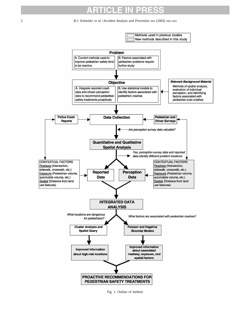
Fig. 1. Outline of method.

R.J. Schneider et al. / Accident Analysis and Prevention xxx (2003) xxx–xxx 3

of perceived high-risk areas and the locations of actual re-ported crash data. If the two point patterns are from two dif-ferent spatial distributions then we may safely assume thatperception data could add some important information aboutthe environmental factors associated with pedestrian-autocrashes, such as roadway features, exposure, etc. It is likelythat the locations of both actual and perceived pedestrianrisk depend on a combination of physical/environmental, aswell as, individual factors. Physical/environmental factorsinclude the presence of sidewalks, traffic, and roadway cross-ings, while individual factors include the ability to judge dis-tance and speed, visual capabilities, and the physical abilityto move quickly and change direction.

Our second objective is then to analyze the factors fromboth geographic distributions through a regression analysis.Our analysis focuses on several specific, measurable phys-ical/environmental factors that can be changed through en-gineering, education, and enforcement policies to improvepedestrian conditions (prevent crashes and improve percep-tions of safety). Therefore, the methodology outlined in thispaper could be used by decision makers as a tool to se-lect appropriate pedestrian crash countermeasures at key lo-cations (Fig. 1). By including the factors from perceivedhigh-risk locations we are taking a proactive approach thatmight avoid an accident “waiting to happen.”

2. Previous safety research on perception andspatial analysis

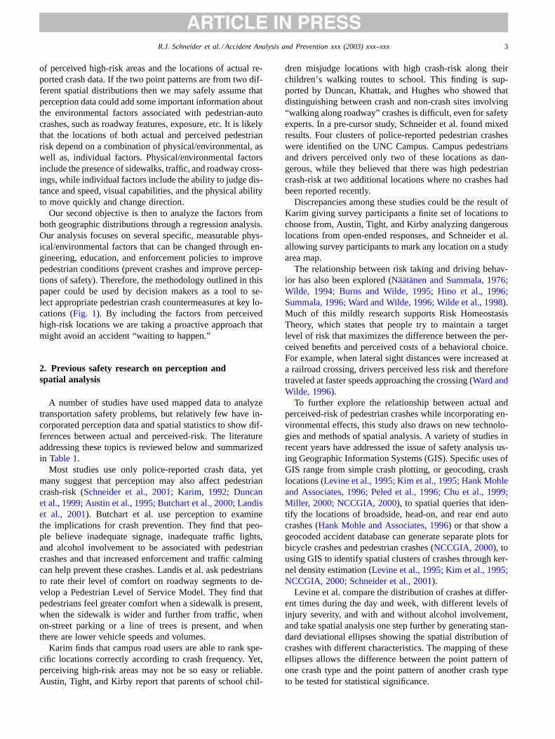
A number of studies have used mapped data to analyzetransportation safety problems, but relatively few have in-corporated perception data and spatial statistics to show dif-ferences between actual and perceived-risk. The literatureaddressing these topics is reviewed below and summarizedin Table 1.

Most studies use only police-reported crash data, yetmany suggest that perception may also affect pedestriancrash-risk (Schneider et al., 2001; Karim, 1992; Duncanet al., 1999; Austin et al., 1995; Butchart et al., 2000; Landiset al., 2001). Butchart et al. use perception to examinethe implications for crash prevention. They find that peo-ple believe inadequate signage, inadequate traffic lights,and alcohol involvement to be associated with pedestriancrashes and that increased enforcement and traffic calmingcan help prevent these crashes. Landis et al. ask pedestriansto rate their level of comfort on roadway segments to de-velop a Pedestrian Level of Service Model. They find thatpedestrians feel greater comfort when a sidewalk is present,when the sidewalk is wider and further from traffic, whenon-street parking or a line of trees is present, and whenthere are lower vehicle speeds and volumes.

Karim finds that campus road users are able to rank spe-cific locations correctly according to crash frequency. Yet,perceiving high-risk areas may not be so easy or reliable.Austin, Tight, and Kirby report that parents of school chil-

dren misjudge locations with high crash-risk along theirchildren’s walking routes to school. This finding is sup-ported by Duncan, Khattak, and Hughes who showed thatdistinguishing between crash and non-crash sites involving“walking along roadway” crashes is difficult, even for safetyexperts. In a pre-cursor study, Schneider et al. found mixedresults. Four clusters of police-reported pedestrian crasheswere identified on the UNC Campus. Campus pedestriansand drivers perceived only two of these locations as dan-gerous, while they believed that there was high pedestriancrash-risk at two additional locations where no crashes hadbeen reported recently.

Discrepancies among these studies could be the result ofKarim giving survey participants a finite set of locations tochoose from, Austin, Tight, and Kirby analyzing dangerouslocations from open-ended responses, and Schneider et al.allowing survey participants to mark any location on a studyarea map.

The relationship between risk taking and driving behav-ior has also been explored (Näätänen and Summala, 1976;Wilde, 1994; Burns and Wilde, 1995; Hino et al., 1996;Summala, 1996; Ward and Wilde, 1996; Wilde et al., 1998).Much of this mildly research supports Risk HomeostasisTheory, which states that people try to maintain a targetlevel of risk that maximizes the difference between the per-ceived benefits and perceived costs of a behavioral choice.For example, when lateral sight distances were increased ata railroad crossing, drivers perceived less risk and thereforetraveled at faster speeds approaching the crossing (Ward andWilde, 1996).

To further explore the relationship between actual andperceived-risk of pedestrian crashes while incorporating en-vironmental effects, this study also draws on new technolo-gies and methods of spatial analysis. A variety of studies inrecent years have addressed the issue of safety analysis us-ing Geographic Information Systems (GIS). Specific uses ofGIS range from simple crash plotting, or geocoding, crashlocations (Levine et al., 1995; Kim et al., 1995; Hank Mohleand Associates, 1996; Peled et al., 1996; Chu et al., 1999;Miller, 2000; NCCGIA, 2000), to spatial queries that iden-tify the locations of broadside, head-on, and rear end autocrashes (Hank Mohle and Associates, 1996) or that show ageocoded accident database can generate separate plots forbicycle crashes and pedestrian crashes (NCCGIA, 2000), tousing GIS to identify spatial clusters of crashes through ker-nel density estimation (Levine et al., 1995; Kim et al., 1995;NCCGIA, 2000; Schneider et al., 2001).

Levine et al. compare the distribution of crashes at differ-ent times during the day and week, with different levels ofinjury severity, and with and without alcohol involvement,and take spatial analysis one step further by generating stan-dard deviational ellipses showing the spatial distribution ofcrashes with different characteristics. The mapping of theseellipses allows the difference between the point pattern ofone crash type and the point pattern of another crash typeto be tested for statistical significance.

4R

.J.S

chn

eid

er

et

al./A

ccide

nt

An

alysis

an

dP

reven

tion

xxx(2

00

3)

xxx–xxx

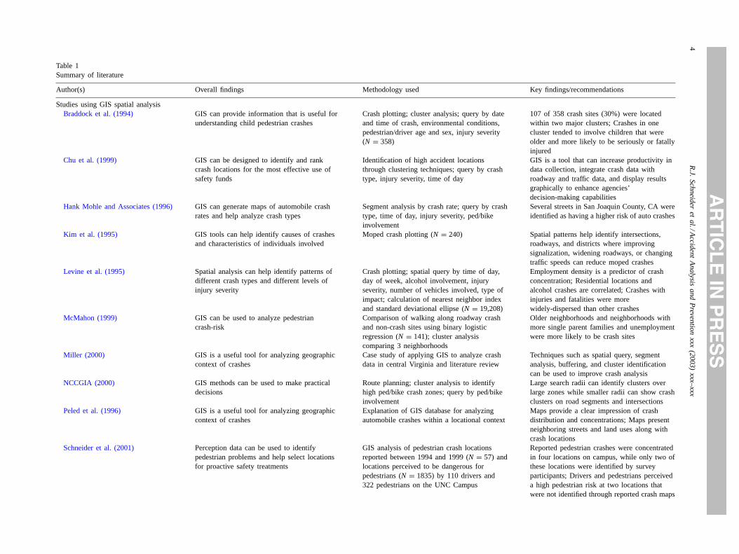
Table 1Summary of literature

Author(s) Overall findings Methodology used Key findings/recommendations

Studies using GIS spatial analysisBraddock et al. (1994) GIS can provide information that is useful for

understanding child pedestrian crashesCrash plotting; cluster analysis; query by dateand time of crash, environmental conditions,pedestrian/driver age and sex, injury severity(N = 358)

107 of 358 crash sites (30%) were locatedwithin two major clusters; Crashes in onecluster tended to involve children that wereolder and more likely to be seriously or fatallyinjured

Chu et al. (1999) GIS can be designed to identify and rankcrash locations for the most effective use ofsafety funds

Identification of high accident locationsthrough clustering techniques; query by crashtype, injury severity, time of day

GIS is a tool that can increase productivity indata collection, integrate crash data withroadway and traffic data, and display resultsgraphically to enhance agencies’decision-making capabilities

Hank Mohle and Associates (1996) GIS can generate maps of automobile crashrates and help analyze crash types

Segment analysis by crash rate; query by crashtype, time of day, injury severity, ped/bikeinvolvement

Several streets in San Joaquin County, CA wereidentified as having a higher risk of auto crashes

Kim et al. (1995) GIS tools can help identify causes of crashesand characteristics of individuals involved

Moped crash plotting (N = 240) Spatial patterns help identify intersections,roadways, and districts where improvingsignalization, widening roadways, or changingtraffic speeds can reduce moped crashes

Levine et al. (1995) Spatial analysis can help identify patterns ofdifferent crash types and different levels ofinjury severity

Crash plotting; spatial query by time of day,day of week, alcohol involvement, injuryseverity, number of vehicles involved, type ofimpact; calculation of nearest neighbor indexand standard deviational ellipse (N = 19,208)

Employment density is a predictor of crashconcentration; Residential locations andalcohol crashes are correlated; Crashes withinjuries and fatalities were morewidely-dispersed than other crashes

McMahon (1999) GIS can be used to analyze pedestriancrash-risk

Comparison of walking along roadway crashand non-crash sites using binary logisticregression (N = 141); cluster analysiscomparing 3 neighborhoods

Older neighborhoods and neighborhoods withmore single parent families and unemploymentwere more likely to be crash sites

Miller (2000) GIS is a useful tool for analyzing geographiccontext of crashes

Case study of applying GIS to analyze crashdata in central Virginia and literature review

Techniques such as spatial query, segmentanalysis, buffering, and cluster identificationcan be used to improve crash analysis

NCCGIA (2000) GIS methods can be used to make practicaldecisions

Route planning; cluster analysis to identifyhigh ped/bike crash zones; query by ped/bikeinvolvement

Large search radii can identify clusters overlarge zones while smaller radii can show crashclusters on road segments and intersections

Peled et al. (1996) GIS is a useful tool for analyzing geographiccontext of crashes

Explanation of GIS database for analyzingautomobile crashes within a locational context

Maps provide a clear impression of crashdistribution and concentrations; Maps presentneighboring streets and land uses along withcrash locations

Schneider et al. (2001) Perception data can be used to identifypedestrian problems and help select locationsfor proactive safety treatments

GIS analysis of pedestrian crash locationsreported between 1994 and 1999 (N = 57) andlocations perceived to be dangerous forpedestrians (N = 1835) by 110 drivers and322 pedestrians on the UNC Campus

Reported pedestrian crashes were concentratedin four locations on campus, while only two ofthese locations were identified by surveyparticipants; Drivers and pedestrians perceiveda high pedestrian risk at two locations thatwere not identified through reported crash maps

R.J.

Sch

ne

ide

re

ta

l./Accid

en

tA

na

lysisa

nd

Preve

ntio

nxxx

(20

03

)xxx–

xxx5

Table 1 (Continued)

Author(s) Overall findings Methodology used Key findings/recommendations

Studies incorporating perceptionAustin et al. (1995) Parents do not perceive dangerous walking

locations correctlySimple analysis of parental survey thatidentified locations of safety concern on kids’routes to school (N = unreported)

Unsafe locations identified in parentalcomments did not correspond closely toreported accident locations

Butchart et al. (2000) Perception of pedestrian injury risk can beused for crash prevention

Survey of households in six neighborhoods ina low income area of Johannesburg, SouthAfrica (N = 1075)

Inadequate signage, traffic lights+ alcoholinvolvement were perceived as pedestrian riskfactors; Increased enforcement+ trafficcalming were perceived as preventativemeasures

Duncan et al. (1999) Perception of safety is difficult, even for experts Delphi process in which five pedestrian safetyexperts attempted to identify crash sites fromamong those with and without crashes (N= 147)

Professionals had difficulty determining crashsites based only on visible physical roadwaycharacteristics

Harrell (1991) Expectations affect driver detection ofpedestrians

Citation of 1985 study by Shinar Drivers detected pedestrians at night more oftenwhen pedestrian encounters were expected

Karim (1992) Road users are aware of accident-pronelocations on campus

Simple statistical analysis of survey responsesregarding accident-prone locations (N= unreported)

Road users ranked specific locations correctlyin terms of crash frequency on survey

Landis et al. (2001) The comfort level of pedestrians on roadwaysegments with different characteristics can bemodeled to create a pedestrian level of service

Stepwise multivariate regression estimatedeffect of sidewalk presence, lateral separationof pedestrians from roadway traffic, drivewayfrequency, and vehicle mix, volume and speedon pedestrian comfort (N = 74 participants,N= 1250 observations,N = 42 directionalroadway segments)

Pedestrian convenience and comfort increasewhen a sidewalk is present, when the sidewalkis wider and further from traffic, when on-streetparking or a line of trees is present, and whenthere are lower vehicle speeds and volumes

Schneider et al. (2001) Perception data can be used to identifypedestrian problems and help select locationsfor proactive safety treatments

GIS analysis of pedestrian crash locationsreported between 1994 and 1999 (N = 57) andlocations perceived to be dangerous forpedestrians (N = 1835) by 110 drivers and322 pedestrians on the UNC Campus

Reported pedestrian crashes were concentratedin four locations on campus, while only two ofthese locations were identified by surveyparticipants; Drivers and pedestrians perceiveda high pedestrian risk at two locations thatwere not identified through reported crash maps

N: sample size.

6 R.J. Schneider et al. / Accident Analysis and Prevention xxx (2003) xxx–xxx

2.1. Gaps in the literature

We found no studies that: (a) use quantitative spatialtests to identify clusters of pedestrian crashes; (b) per-form inter-distributional spatial tests to show the differencebetween police-reported crash locations and locations per-ceived to have a high crash-risk; (c) estimate appropriaterigorous models to identify factors associated with pedes-trian crash-risk; or (d) examine the effect of pedestrianexposure on pedestrian crash-risk.

This study attempts to fill some of these gaps by utilizingGIS and spatial analysis capabilities to analyze the spatialdistribution of both actual and perceived pedestrian crash

Fig. 2. UNC-Chapel Hill land use (January 2001).

locations, and then to determine which environmental fac-tors, including nearby land uses, may have an effect on theiroccurrence.

3. Description of study area and data collection

Our technique of integrating police-reported crash datawith perception survey data was tested on the campus ofthe University of North Carolina at Chapel Hill, a 300-ha(740-acre) area that is home to over 23,000 students, 2800faculty, and many other employees (Peterson’s, 2000). Thegeographic distribution of land uses on the UNC Campus

R.J. Schneider et al. / Accident Analysis and Prevention xxx (2003) xxx–xxx 7

makes the campus an excellent area to study the spatial re-lationships between pedestrian problems and pedestrian andvehicle flows, development character, and activity destina-tions. Like many other college campuses, the UNC Campusstreets contain a mix of pedestrians, bicycles, and automo-biles. Conflicts between pedestrians and vehicles occur as

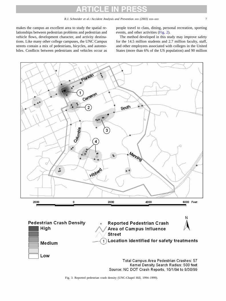
Fig. 3. Reported pedestrian crash density (UNC-Chapel Hill, 1994–1999).

people travel to class, dining, personal recreation, sportingevents, and other activities (Fig. 2).

The method developed in this study may improve safetyfor the 14.5 million students and 2.7 million faculty, staff,and other employees associated with colleges in the UnitedStates (more than 6% of the US population) and 90 million

8 R.J. Schneider et al. / Accident Analysis and Prevention xxx (2003) xxx–xxx

college students and teachers worldwide, many of whomwalk on campuses (US Department of Education, 2000).In addition, the method presented here can be applied toneighborhoods, commercial areas, and other locales withlarge numbers of pedestrians.

3.1. Spatial data

There were 57 police-reported collisions between vehi-cles and pedestrians on the UNC Campus between October1994 and September 1999. Reports for each of these crasheswere extracted from the state crash database and the crash

Fig. 4. Perception of pedestrian crash-risk (locations perceived to have a high-risk of pedestrian crashes by pedestrians and drivers on UNC-ChapelHillCampus).

locations were geocoded on a GIS map with an accuracyof better than 30 m (100 ft) (this was the level of measure-ment accuracy used in the police reports). UsingCrimeStat,a spatial statistics software package (Levine, 1999), the datarevealed four main clusters of crashes.Fig. 3 shows theseclusters and the density of crashes associated with them asdetermined through kernel estimation.

A perception survey was also designed to gather addi-tional data about locations where pedestrian safety problemscould exist on campus. Four hundred fifty pedestrian sur-veys were mailed to a random list of students, faculty, andother employees, and 510 driver surveys were mailed to a

R.J. Schneider et al. / Accident Analysis and Prevention xxx (2003) xxx–xxx 9

random list of people with campus parking permits. Over21% of each group responded. Two hundred fifteen extrapedestrian surveys were given in person at five locations oncampus. Though people may have been more likely to marklocations near where the surveys were distributed, pedes-trians were over-sampled to ensure that people who walkin all areas of campus were selected. Because it was likelythat most pedestrian survey participants had also driven oncampus and that most people taking the driver survey hadalso walked on campus, the pedestrian survey participantswere instructed to complete the survey from their perspec-tive as a pedestrian, and driver survey participants wereasked to complete the survey from their perspective as adriver. In all, 312 pedestrian and 110 driver surveys wereanalyzed.

The surveys included two identical maps of the cam-pus area. Participants used the first map to mark the threelocations that they believed had the highest risk of pedes-trian crashes during daylight. If participants felt that therisk of pedestrian crashes on campus changed at night,they marked the three locations with the highest risk ofpedestrian crashes during darkness on a second map. Thisnumber of locations was required so that there would beadequate variation in locations if all respondents agreedthat one location was the most dangerous point on campus,and that the number of locations would be small enoughfor respondents to think of and mark on the survey quickly.Yet, some respondents still marked only one or two loca-tions. In all, the 422 pedestrians and drivers provided 1835locations (data points) on campus that were perceived tohave a high-risk of pedestrian crashes (compared to only 57police-reported crash locations). Twenty-seven off-campuslocations were also marked, but these were not used in fur-ther analyses. Because there were only minor differencesbetween locations identified during daylight and darkness,the 1835 locations identified in the surveys were combinedto create a composite map representing the perception ofpedestrian crash-risk on campus (Fig. 4).

4. Reported crashes and risk perception: comparingpoint distributions

If no difference is found between the spatial distribu-tion of perceived pedestrian risk and the police-reportedcrash-risk, the survey data would add little value in iden-tifying future crash locations. However, even a visual com-parison ofFigs. 3 and 4shows that there are differencesbetween the locations of police-reported crashes and the lo-cations where pedestrians and drivers perceived pedestriancrash problems on the UNC Campus. This visual assessmentmust be supported by statistical methods to reveal whetherthe differences between the two point distributions are sig-nificant. We use two quantitative techniques (Chi-squaredand nearest neighbor cluster analyses) to test the null hy-pothesis thatthe spatial distribution of risk perceptions is

not significantly different from the spatial distribution ofpolice-reported pedestrian crash locations.

4.1. A note about estimating surfaces

We use kernel density estimation to create a probabil-ity surface of crashes. Both the kernel density and nearestneighbor cluster analyses assume complete spatial random-ness, which implies that there is the potential for reportedand perceived pedestrian crash-risk across the entire mapsurface, i.e. in buildings and in other open spaces awayfrom the roadway network. Though this assumption cannotrealistically be made, the purpose of the spatial testing isto show the differences in the actual and perceived-riskdistributions. Since the point distributions are naturallyconstrained to the same roadway network (crashes occurredon roadways, at intersections, and in parking lots, and peo-ple marked risky locations on roadways, at intersections,and in parking lots), the crash-risk that is estimated is alsoconstrained along the roadways and, therefore the spatialcomparisons presented here are appropriate.

4.2. Chi-squared analysis

The first statistical test used is a Chi-squared test,which examines the relationshipbetweenpoints in eachdistribution (Taylor, 1977; Getis and Boots, 1978). Thisinter-distributional test shows whether the total counts ofpolice-reported crashes and the points perceived as danger-ous on each of the 94 campus roadway network segmentsor intersections can be classified into similar ranges, andtherefore, are distributed similarly. Note that the test doesnot account for the location of each segment/intersection,but it is an appropriate test to make an initial comparison be-tween both point distributions along the network segments.Each of the 94 campus roadway segments/intersections areclassified as having 0, 1, 2, or at least 3 reported crashes.This classification is then compared to the expected num-ber of crashes on each segment/intersection if the crasheswere distributed in the same spatial pattern as the perceiveddangerous locations.

This parallel classification scheme allows a Chi-squaredstatistic to be calculated:

χ2 =n∑

i=1

(Oir − Oie)2

Oie

(1)

where i represents each of the four categories (0, 1, 2,or at least 3 or more police-reported crashes),Oir is thenumber of segments/intersections falling into categoryiaccording to the number of police-reported crashes on thesegment/intersection, andOie is the expected number ofsegments/intersections that would fall into categoryi if thepolice-reported crashes were spatially distributed on theroadway segments/intersections in the same manner as the

10 R.J. Schneider et al. / Accident Analysis and Prevention xxx (2003) xxx–xxx

perception survey responses. The test is also performedusing the perception data as a base:

χ2 =n∑

i=1

(Oip − Oie)2

Oie

(2)

wherei represents each of the five categories (0–29, 30–59,60–89, 90–119, or 120 or more perception points) andOip

is the number of segments/intersections falling into cate-gory i according to the number of perception points on thesegment/intersection.

4.3. Chi-squared results

Both Chi-squared tests showed that the counts of crashesand risk-perception locations on each segment/intersectionwere distributed into different categories. When the expectednumber of police-reported crashes on each roadway seg-ment/intersection was based on the distribution of locationsperceived to be dangerous, the Chi-squared value was 46.4with three degrees of freedom (Table 2). Therefore, we are99.9% confident that there are differences in the manner inwhich reported and perceived dangerous locations are dis-tributed on the campus roadway intersections and segments.Similarly, a Chi-squared value of 14.5 with four degrees offreedom was generated when the expected number of loca-tions perceived to be dangerous on each segment/intersectionwas based on the number of police-reported crashes, mean-ing that the two distributions were significantly different atthe 99.0% level.

Table 2Chi-squared test (N = 94 segments/intersections)

i, class (number of reported crashes onsegment/intersection)

Oir , number ofsegments in classi

Oie, expected number of segments in classi if reported crashes weredistributed in same spatial pattern as perception locations

Reported crash data(χ2 = ∑n

i=1(Oir − Oie)2/Oie

)0 ≤ x < 1 59 801 ≤ x < 2 22 102 ≤ x < 3 9 2x ≥ 3 4 2

Total 94 94

χ2 46.4d.f. 3α(0.001) 16.3

i, class (number of perception locations onsegment/intersection)

Oip, number ofsegments in classi

Oie, expected number of segments in classi if perception locationswere distributed in same spatial pattern as reported crashes

Perception data(χ2 = ∑n

i=1(Oip − Oie)2/Oie

)0 ≤ x < 30 76 5930 ≤ x < 60 13 2260 ≤ x < 90 2 990 ≤ x < 120 1 2x ≥ 120 2 2

Total 94 94

χ2 14.5d.f. 4α(0.01) 13.3

Though these differences did not account for the spatial ar-rangement of the segments/intersections, this result showedthat some parts of the campus roadway network with largerproportions of police-reported crashes were not matchedwith a large proportion of perception survey responses (suchas the intersection of Franklin Street and Columbia Street)and that specific areas with large proportions of survey re-sponses had few crashes reported in the last 5 years (such asthe segment of Manning Drive to the east of its intersectionwith Columbia Street).

4.4. Nearest neighbor cluster analysis

The second type of spatial comparison, nearest neighboranalysis, is used to identify clusters of points within eachspatial distribution. After they are identified, the clusters ofone distribution are compared with clusters of the other dis-tribution. This intra-distributional technique uses Euclideandistance to identify sets of points that are clustered moreclosely than would be expected by random chance. Pointsare considered clustered when the mean random distancebetween them is less than a minimum distance based on thestandard error of a random distribution:

minimum distance= 0.5

√A

N− t

[0.26136√

N2/A

](3)

whereA is the area of the study region,N is the number ofcrash locations (N = 57) or locations perceived to be dan-gerous (N = 1835),t is a probability level in the Student’st-distribution, and [0.26136/(

√N2/A)] is the standard error

R.J. Schneider et al. / Accident Analysis and Prevention xxx (2003) xxx–xxx 11

distance of a random distribution (Levine, 1999). In otherwords, for a one-tailed probability,P, fewer thanP percentof the points would have nearest neighbor distances less thanthis lower limit if the point distribution was completely ran-dom. For this analysis we use aP-value of 0.01 so that wecan be 99% confident that the police-reported and percep-tion location clusters did not occur by random chance. Theminimum number of points required to make a cluster is setat three reported crashes and 40 locations perceived to bedangerous.

The standard deviational ellipse of each nearest neigh-bor cluster and the number of points they contain are alsoreported. The standard deviational ellipse measures the dis-persion and orientation of the points around the mean cen-ter (mean latitude, mean longitude) of the cluster. Equa-tions for drawing standard deviational ellipses are presentedby Levine (1999). Similarity between the two distributionsis demonstrated when the standard deviational ellipses ofthe police-reported crash clusters overlap corresponding per-ceived location cluster ellipses. Yet, if the standard devia-tional ellipse of a reported crash cluster does not contain themean center of the closest cluster of perceived locations, wecan be 99% confident that the two types of data are identi-fying different locations with pedestrian problems.

4.5. Nearest neighbor cluster results

Cluster analysis revealed notable differences betweenconcentrations of reported crashes and locations perceivedto be dangerous (Fig. 5). Only three police-reported crashclusters were identified at the 99% significance level us-ing the nearest neighbor cluster method. In contrast, therewere six clusters of perception locations. The relationshipbetween location and size of the clusters of police-reportedcrashes and clusters of locations perceived to be dangerousis important to note. At the intersection of Franklin Streetand Columbia Street, the center of the cluster of nine re-ported crashes and center of the perceived location clusterwere within 12 m (40 ft) of each other and their standarddeviational ellipses overlapped. This means that the percep-tions of pedestrians and drivers verified reported pedestrianproblems at that intersection. Yet, neither of the other twoclusters of reported crashes corresponded closely to a clusterof locations perceived to be dangerous. Though the clusterof five reported crashes on South Road was only 100 m(320 ft) from a cluster of locations perceived to be danger-ous on South Road, their standard deviational ellipses didnot overlap (Fig. 5). Therefore, we are 99% confident thatthey refer to different locations of pedestrian problems. Theperception cluster is centered on the crosswalk between theStudent Union and Student Recreation Center, while thepolice-reported crash cluster may represent general prob-lems in the vicinity of South Road. The final cluster of fourreported crashes was located off Manning Drive near thehospital complex, but its standard deviational ellipse didnot overlap with either cluster of locations perceived to be

dangerous on Manning Drive. We conclude that the clustersgenerated by the police-reported crash locations and loca-tions perceived to be dangerous provide further evidencethat the two data sets have different spatial characteristics.

4.6. Spatial testing summary

Several other spatial statistics were used to test for sig-nificant differences between reported and perceived-riskpoint patterns. Though they are not reported here, Ripley’sK-function (Bailey and Gatrell, 1995; Levine, 1999) anda G-function (Bailey and Gatrell, 1995) also revealedsignificant differences between the locations of the twodistributions.

Overall, the spatial analyses show that some locations ofreported pedestrian crashes are identified accurately by per-ception survey participants, while there is also evidence of a“perception mismatch” between clusters of reported crashesand perceived pedestrian crash-risk. Based on the results ofthis spatial analysis, there are statistically significant dif-ferences between the distribution of police-reported crashesand the distribution of locations perceived to be dangerous,implying that risk-perception data can be valuable in proac-tive pedestrian planning.

4.7. Applying perception mismatch to crash prevention

The “perception mismatch” between police-reportedcrash and survey locations has implications for crash pre-vention. Recommendations can be made for four differenttypes of locations:

(1) High reported and high perceived-risk: Top-priority ar-eas for engineering, education, and enforcement treat-ments.

(2) High reported and low perceived-risk: Both engineer-ing and education improvements should be explored.These are locations where there is a physical problemyet people are not aware of the danger. The physicalaspect of the problem can be treated with engineeringchanges, and the awareness aspect can be treated by ed-ucating drivers and pedestrians. Note that education maybe implemented much more quickly than an engineer-ing treatment, which may have to go through a CapitalImprovement Program before being made.

(3) Low reported and high perceived-risk: Evaluate theseareas to see if pedestrian and driver experience hasaccurately identified existing and potential problems. Ifproblems are found, it may be possible to treat the sitesproactively with appropriate engineering, education, andenforcement measures to prevent future pedestriancrashes.

(4) Low reported and low perceived-risk: No countermea-sures necessary, but continue normal monitoring.

Note that it is possible that people simply do not useor they walk with extreme caution in areas where there is

12R

.J.S

chn

eid

er

et

al./A

ccide

nt

An

alysis

an

dP

reven

tion

xxx(2

00

3)

xxx–xxx

Fig. 5. Cluster analysis. Nearest neighbor clusters (UNC Campus reported crash locations vs. locations perceived to be dangerous).

R.J. Schneider et al. / Accident Analysis and Prevention xxx (2003) xxx–xxx 13

extreme danger (i.e. high-speed arterials, multi-lane road-ways, streets with high traffic and no sidewalks, etc.).We emphasize that our methodology is most useful forsituations and areas where there is a moderate perceivedcrash-risk (common on campuses, in neighborhoods, and incommercial areas). Depending on their ability to confrontdanger (which may be affected by age, weather, drugs, etc.),pedestrians may walk in these moderate-risk locations. Evenpedestrians who perceive danger, but may not take unwar-ranted risks, can suggest where crashes may occur to others.Further, speeding or reckless drivers who are unaware ofpedestrians may cause pedestrian crashes, no matter howcareful the pedestrians are when they are in the roadway.Therefore, it is useful to know about the locations wherepedestrians perceive danger—it is locations like these wherepedestrian crashes could occur in the future if engineering,education, and enforcement treatments are not made.

It is especially important to identify risky locations proac-tively for pedestrians because pedestrian injuries are oftenmuch more severe when accidents occur. In locations thathave experienced no pedestrian crashes, the very first crashcan be fatal, as we saw on the UNC Campus. In addition,perceived-risk can be used for more than a superficial ex-amination of personal ability to “read” the safety of the en-vironment. The perception survey and resulting maps canbe shared with the public to point out specific locations asbeing dangerous and in need of attention.

5. Modeling reported and perceived crash-risk

On the UNC Campus, reported crash locations do notcorrespond closely to perception survey locations near theUNC Hospital and south of Manning Drive; perception sur-vey locations do not correspond closely to police-reportedcrash locations along parts of Cameron Street and onColumbia Street between South Road and Manning Drive(compareFigs. 3 and 4). The spatial pattern of “perceptionmismatch” requires further investigation. A richer under-standing of this spatial pattern can be obtained by exam-ining the combinations of pedestrian and vehicle volumes,roadway features, and nearby land uses that may be under-lying physical/environmental causes of pedestrian crashesand risk perception.

We use Poisson and negative binomial crash models toshow the exposure, roadway, and land use factors that arerelated significantly (at least at the 90% confidence level) tothe police-reported and perceived-risk of pedestrian crashes.Incorporating these geographic/land use factors in the re-gression modeling process demonstrates the connectivitybetween spatial and multivariate crash analysis.

5.1. Regression model data

The campus roadway network is divided into 38 inter-sections (nodes, defined as the area within 15 m (50 ft) of

the intersection of two or more roadway center lines) and56 segments (links, defined as lengths of roadway betweenintersections), each of which are assigned specific pedes-trian crash-risk, exposure, roadway, and land use charac-teristics. These 94 units of analysis will be referred to assegments/intersections in the following sections. By con-sidering the geographic context of the UNC Campus, thisstudy shows that exposure, physical roadway, andspatialcharacteristicsare related to pedestrian safety problems.

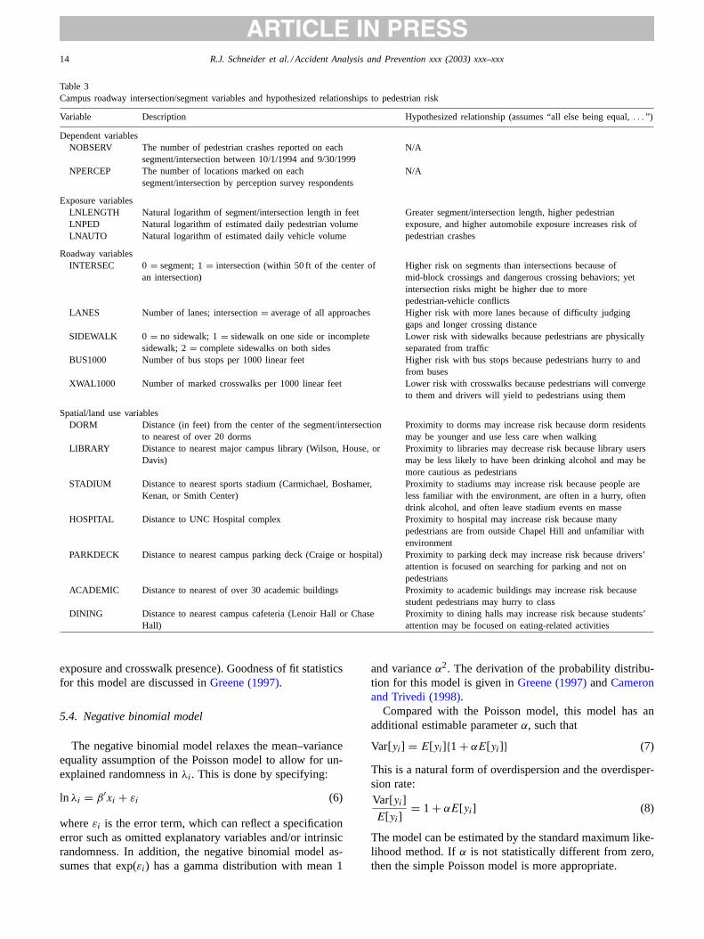
Three exposure, five roadway, and seven land use char-acteristics were collected for each segment/intersectionfrom traffic and pedestrian volume maps, field observation,and GIS measurement. Descriptions of these variables andtheir hypothesized relationships to pedestrian crash-risk(represented by the number of reported crashes or numberof perceived locations on each segment/intersection) arepresented inTable 3.

5.2. Regression models

The Poisson statistical distribution represents the occur-rence of “infrequent events.” Therefore, Poisson modeling isappropriate for modeling the number, or count, of actual orperceived crash locations on each campus roadway intersec-tion/segment. However, the Poisson model requires that themean equal the variance of the count data. The negative bi-nomial regression model can relax the mean–variance equal-ity assumption (Greene, 1997; Cameron and Trivedi, 1998).The difference between the means and variances of reportedcrashes (mean= 0.606, variance= 1.44) and locations per-ceived as dangerous (mean= 19.5, variance= 946) is rela-tively large, favoring the negative binomial model. However,for comparison, both Poisson and negative binomial modelsare presented.

5.3. Poisson model

The Poisson model usesYi to denote the number of crashoccurrences or locations perceived to be dangerous for theith of N = 94 campus roadway segments/intersections.This number of crash occurrences on each element can bePoisson distributed with probability density:

P [Yi = yi] = eλiλyi

i

yi!(4)

where λi is the segment/intersectioni’s expected crashfrequency;yi = 0, 1, 2,. . . (realized value of the crash fre-quency); andi = 1, 2, . . . , N andyi! denotes the factorialof yi. Note that the mean and variance ofYi equalsλi.

To incorporate explanatory variablesxi the parameterλi

is specified to be

λi = exp(β′xi) (5)

whereβ′ is the vector of estimated parameters; andxi is theroadway elementi’s explanatory variables (e.g. pedestrian

14 R.J. Schneider et al. / Accident Analysis and Prevention xxx (2003) xxx–xxx

Table 3Campus roadway intersection/segment variables and hypothesized relationships to pedestrian risk

Variable Description Hypothesized relationship (assumes “all else being equal,. . . ”)

Dependent variablesNOBSERV The number of pedestrian crashes reported on each

segment/intersection between 10/1/1994 and 9/30/1999N/A

NPERCEP The number of locations marked on eachsegment/intersection by perception survey respondents

N/A

Exposure variablesLNLENGTH Natural logarithm of segment/intersection length in feet Greater segment/intersection length, higher pedestrian

exposure, and higher automobile exposure increases risk ofpedestrian crashes

LNPED Natural logarithm of estimated daily pedestrian volumeLNAUTO Natural logarithm of estimated daily vehicle volume

Roadway variablesINTERSEC 0= segment; 1= intersection (within 50 ft of the center of

an intersection)Higher risk on segments than intersections because ofmid-block crossings and dangerous crossing behaviors; yetintersection risks might be higher due to morepedestrian-vehicle conflicts

LANES Number of lanes; intersection= average of all approaches Higher risk with more lanes because of difficulty judginggaps and longer crossing distance

SIDEWALK 0 = no sidewalk; 1= sidewalk on one side or incompletesidewalk; 2= complete sidewalks on both sides

Lower risk with sidewalks because pedestrians are physicallyseparated from traffic

BUS1000 Number of bus stops per 1000 linear feet Higher risk with bus stops because pedestrians hurry to andfrom buses

XWAL1000 Number of marked crosswalks per 1000 linear feet Lower risk with crosswalks because pedestrians will convergeto them and drivers will yield to pedestrians using them

Spatial/land use variablesDORM Distance (in feet) from the center of the segment/intersection

to nearest of over 20 dormsProximity to dorms may increase risk because dorm residentsmay be younger and use less care when walking

LIBRARY Distance to nearest major campus library (Wilson, House, orDavis)

Proximity to libraries may decrease risk because library usersmay be less likely to have been drinking alcohol and may bemore cautious as pedestrians

STADIUM Distance to nearest sports stadium (Carmichael, Boshamer,Kenan, or Smith Center)

Proximity to stadiums may increase risk because people areless familiar with the environment, are often in a hurry, oftendrink alcohol, and often leave stadium events en masse

HOSPITAL Distance to UNC Hospital complex Proximity to hospital may increase risk because manypedestrians are from outside Chapel Hill and unfamiliar withenvironment

PARKDECK Distance to nearest campus parking deck (Craige or hospital) Proximity to parking deck may increase risk because drivers’attention is focused on searching for parking and not onpedestrians

ACADEMIC Distance to nearest of over 30 academic buildings Proximity to academic buildings may increase risk becausestudent pedestrians may hurry to class

DINING Distance to nearest campus cafeteria (Lenoir Hall or ChaseHall)

Proximity to dining halls may increase risk because students’attention may be focused on eating-related activities

exposure and crosswalk presence). Goodness of fit statisticsfor this model are discussed inGreene (1997).

5.4. Negative binomial model

The negative binomial model relaxes the mean–varianceequality assumption of the Poisson model to allow for un-explained randomness inλi. This is done by specifying:

ln λi = β′xi + εi (6)

whereεi is the error term, which can reflect a specificationerror such as omitted explanatory variables and/or intrinsicrandomness. In addition, the negative binomial model as-sumes that exp(εi) has a gamma distribution with mean 1

and varianceα2. The derivation of the probability distribu-tion for this model is given inGreene (1997)andCameronand Trivedi (1998).

Compared with the Poisson model, this model has anadditional estimable parameterα, such that

Var[yi] = E[yi]{1 + αE[yi]} (7)

This is a natural form of overdispersion and the overdisper-sion rate:Var[yi]

E[yi]= 1 + αE[yi] (8)

The model can be estimated by the standard maximum like-lihood method. Ifα is not statistically different from zero,then the simple Poisson model is more appropriate.

R.J. Schneider et al. / Accident Analysis and Prevention xxx (2003) xxx–xxx 15

5.5. Regression modeling process

With 57 crashes reported on 94 segments/intersectionsin 5 years, a single pedestrian crash on one of the seg-ments/intersections has a large influence on the statis-tical significance of its exposure, roadway, and spatialattributes (there are an average of 0.606 police-reportedcrashes on each segment/intersection, and 63% of the seg-ments/intersections have no crashes). When using percep-tion data, the average segment/intersection has 19.5 markedsurvey locations. Therefore, even if a few respondents over-estimate the risk of future pedestrian crashes at a location,their individual response will not have a large effect on theaccuracy of the perception model. Comparing the factorsfrom these two types of models provides a deeper under-standing of the factors that influence pedestrian crash-risk.

The effects of exposure, roadway, and land use (spa-tial/environmental) factors on reported pedestrian crashlocations and perception of crash-risk were hypothesizedin Table 3. First, separate exposure, roadway, and spatialmodels were estimated. Interaction terms were tested inthese models, but they did not improve their fit. Then, thevariables from the exposure, roadway, and spatial mod-els were used to estimate Poisson and negative binomialcombined models. Finally, the most statistically significantvariables from the combined models were kept and used toestimate refined models. Results from the refined modelsare presented below.

Table 4Poisson and negative binomial models (N = 94)

Independent variable Observed-risk: coefficient, significance level (P) Perceived-risk: coefficient, significance level (P) Mean

Poisson Model 1: Negbin Model 2: Poisson Model 3: Negbin Model 4:

Constant −13.5, (0.0000) −13.5, (0.0033) −19.9, (0.0000) −14.4, (0.0000)Exposure factors

LNLENGTH 0.625, (0.0165) 0.625, (0.0870) 1.05, (0.0000) 0.867, (0.0000) 5.87LNPED 0.672, (0.0091) 0.667, (0.0771) 1.25, (0.0000) 0.871, (0.0000) 7.09LNAUTO 0.381, (0.154) 0.383, (0.262) 1.05, (0.0000) 0.796, (0.0000) 8.85

Roadway factorsINTERSEC −0.935, (0.129) −0.932, (0.276) −0.797, (0.0000) −0.246, (0.451) 0.404SIDEWALK 0.0940, (0.851) 0.101, (0.851) −1.01, (0.0000) −0.697, (0.0029) 1.61BUS1000 −0.159, (0.0958) −0.158, (0.0281) 0.00750, (0.619) 0.0159, (0.774) 1.09XWAL1000 0.0810, (0.0089) 0.0806, (0.0665) 0.090, (0.0000) 0.0643, (0.0002) 5.29

Spatial factorsLIBRARY −0.000841, (0.0685) −0.000822, (0.103) 0.000218, (0.0063) 0.000316, (0.0884) 1910ACADEMIC 0.000996, (0.0599) 0.000973, (0.120) −0.000225, (0.0137) −0.000348, (0.107) 983STADIUM 0.000783, (0.0300) 0.000764, (0.0379) −0.000636, (0.0000) −0.000644, (0.0001) 1690

α 0.0215, (0.944) 0.332, (0.0000)

Summary statisticslog likelihood −83.0 −83.0 −500 −307Restrictive log likelihood −107 −82.978 −1510 −500Goodness of fitR2

p 0.300 0.799Goodness of fitR2

d 0.361 0.763χ2 48.1, (0.0000) 0.0114, (0.915) 2030, (0.0000) 386, (0.0000)

Dependent variable= NOBSERV (µ = 0.606) Dependent variable= NPERCEP (µ = 19.5)

5.6. Regression modeling results

Independent variable coefficients, standard errors, signif-icance levels and overall model summary statistics are pre-sented for the four refined models inTable 4. These fourrefined models include two Poisson (Models 1 and 3) andtwo negative binomial models (Models 2 and 4) estimatingpolice-reported and perceived-risk frequencies.

The Poisson Model 1 is preferred to Model 2 because ithas more significant parameter estimates andα is not sta-tistically significant. However, the negative binomial Model4 is preferred to Model 3 based on goodness-of-fit and thesignificance ofα. Therefore, Models 1 and 4 are discussed,in this order.

As expected, longer segments/intersections and higherpedestrian volumes are significantly related to higher lev-els of police-reported crashes, though higher automobilevolumes are not statistically significant. In addition, theelasticity of the exposure factors is less than one, indicatingthat as length or pedestrian volume increase, the number ofpolice-reported crashes on road segments or intersectionsincrease at a decreasing rate. For example, a one percentincrease in pedestrian volume increases the number ofpolice-reported crashes by 0.672%.

After accounting for exposure, the results show that whensegments/intersections had more marked crosswalks perlinear foot, they had a greater number of police-reportedpedestrian crashes. Though this result is counter to our

16 R.J. Schneider et al. / Accident Analysis and Prevention xxx (2003) xxx–xxx

expectations, it is consistent with studies byHerms (1972)and Zegeer et al. (2001)who find some locations withmarked crosswalks have more pedestrian crashes than con-trol locations without marked crosswalks. However, thisresult does not necessarily suggest that providing markedcrosswalks “causes” pedestrian crashes. Our data does notindicate where the crashes occurred relative to crosswalks.The relation of higher crosswalk density to a higher inci-dence of pedestrian crashes may result from more danger-ous pedestrian or driver behavior in the vicinity of markedcrosswalks, weak crosswalk design, or other factors. Fur-ther study of crosswalks and related behavior is needed toassess the effectiveness of this treatment.

The number of bus stops was statistically significant in thecrash model (90% level), indicating that more bus stops donot create a greater pedestrian crash-risk. The intersectionvariable was not statistically significant in the model. Finally,the number of lanes was statistically non-significant anddropped from the final model specification.

Among spatial factors, proximity to academic buildingsand stadiums is associated with higher crash-risk, whereasproximity to libraries with lower crash-risk. At this point,it is interesting to compare the results of Models 1 and 4.The coefficients for the significant spatial variables in thereported crash model and the perceived-risk model have op-posite signs. Therefore, people perceive less risk near sometypes of land uses where crashes have occurred and per-ceive more risk near other land-uses where no crashes haveoccurred. Locations near the main campus libraries haveexperienced fewer crashes, but they are perceived to havemore danger. In contrast, proximity to academic buildingsincreases police-reported crash-risk but is not perceived todo so. Finally, locations near stadiums are more dangerousaccording to police-reported crash data than people think.The distance from the segments/intersections to the closestdorm, hospital, parking deck, and dining hall were not in-cluded in the refined models because they lacked statisticalsignificance.

The relationship between proximity to certain land usesand crash-risk clearly needs further investigation. Spa-tial/land use factor results may have implications for thedesign of college campuses and neighborhoods. Further re-search could also examine whether a dense traffic networkwith short blocks and many intersections or dense residentialneighborhoods are related to greater actual and perceivedpedestrian risk. Our study used segments and intersectionsas the unit of analysis, so we did not test these relationships.

The results of exposure and roadway factors are quiteconsistent across Models 1 and 4, increasing our confidencein the appropriateness of behavioral data. Though sidewalkpresence was not statistically significant in Model 1, it issignificant in Model 4. The negative coefficient indicatesthat pedestrians and drivers perceived a lower pedestriancrash-risk when more complete sidewalks were provided andmore danger when segments/intersections had incompletesidewalks.

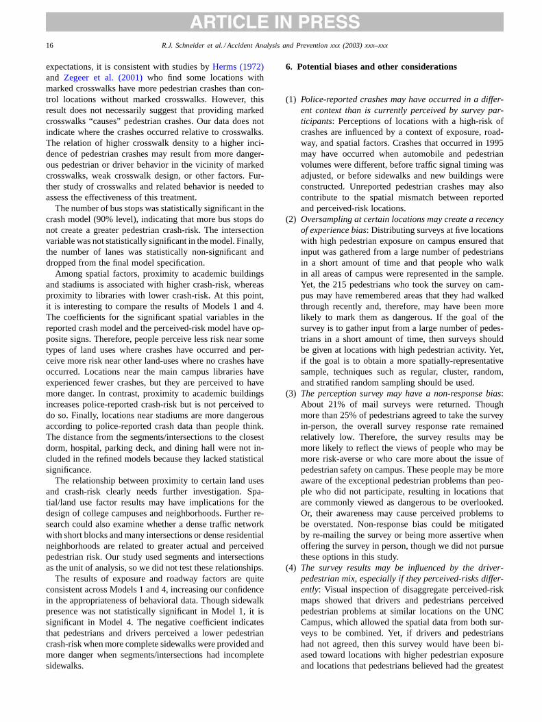
6. Potential biases and other considerations

(1) Police-reported crashes may have occurred in a differ-ent context than is currently perceived by survey par-ticipants: Perceptions of locations with a high-risk ofcrashes are influenced by a context of exposure, road-way, and spatial factors. Crashes that occurred in 1995may have occurred when automobile and pedestrianvolumes were different, before traffic signal timing wasadjusted, or before sidewalks and new buildings wereconstructed. Unreported pedestrian crashes may alsocontribute to the spatial mismatch between reportedand perceived-risk locations.

(2) Oversampling at certain locations may create a recencyof experience bias: Distributing surveys at five locationswith high pedestrian exposure on campus ensured thatinput was gathered from a large number of pedestriansin a short amount of time and that people who walkin all areas of campus were represented in the sample.Yet, the 215 pedestrians who took the survey on cam-pus may have remembered areas that they had walkedthrough recently and, therefore, may have been morelikely to mark them as dangerous. If the goal of thesurvey is to gather input from a large number of pedes-trians in a short amount of time, then surveys shouldbe given at locations with high pedestrian activity. Yet,if the goal is to obtain a more spatially-representativesample, techniques such as regular, cluster, random,and stratified random sampling should be used.

(3) The perception survey may have a non-response bias:About 21% of mail surveys were returned. Thoughmore than 25% of pedestrians agreed to take the surveyin-person, the overall survey response rate remainedrelatively low. Therefore, the survey results may bemore likely to reflect the views of people who may bemore risk-averse or who care more about the issue ofpedestrian safety on campus. These people may be moreaware of the exceptional pedestrian problems than peo-ple who did not participate, resulting in locations thatare commonly viewed as dangerous to be overlooked.Or, their awareness may cause perceived problems tobe overstated. Non-response bias could be mitigatedby re-mailing the survey or being more assertive whenoffering the survey in person, though we did not pursuethese options in this study.

(4) The survey results may be influenced by the driver-pedestrian mix, especially if they perceived-risks differ-ently: Visual inspection of disaggregate perceived-riskmaps showed that drivers and pedestrians perceivedpedestrian problems at similar locations on the UNCCampus, which allowed the spatial data from both sur-veys to be combined. Yet, if drivers and pedestrianshad not agreed, then this survey would have been bi-ased toward locations with higher pedestrian exposureand locations that pedestrians believed had the greatest

R.J. Schneider et al. / Accident Analysis and Prevention xxx (2003) xxx–xxx 17

danger (almost three times as many pedestrian surveyswere analyzed). In such a case, it would be necessaryto generate separate maps and models of pedestrian anddriver perception. The perception mismatch betweenpedestrians and drivers is also important to note be-cause the most dangerous locations may be where oneof these two groups do not perceive a high-risk.

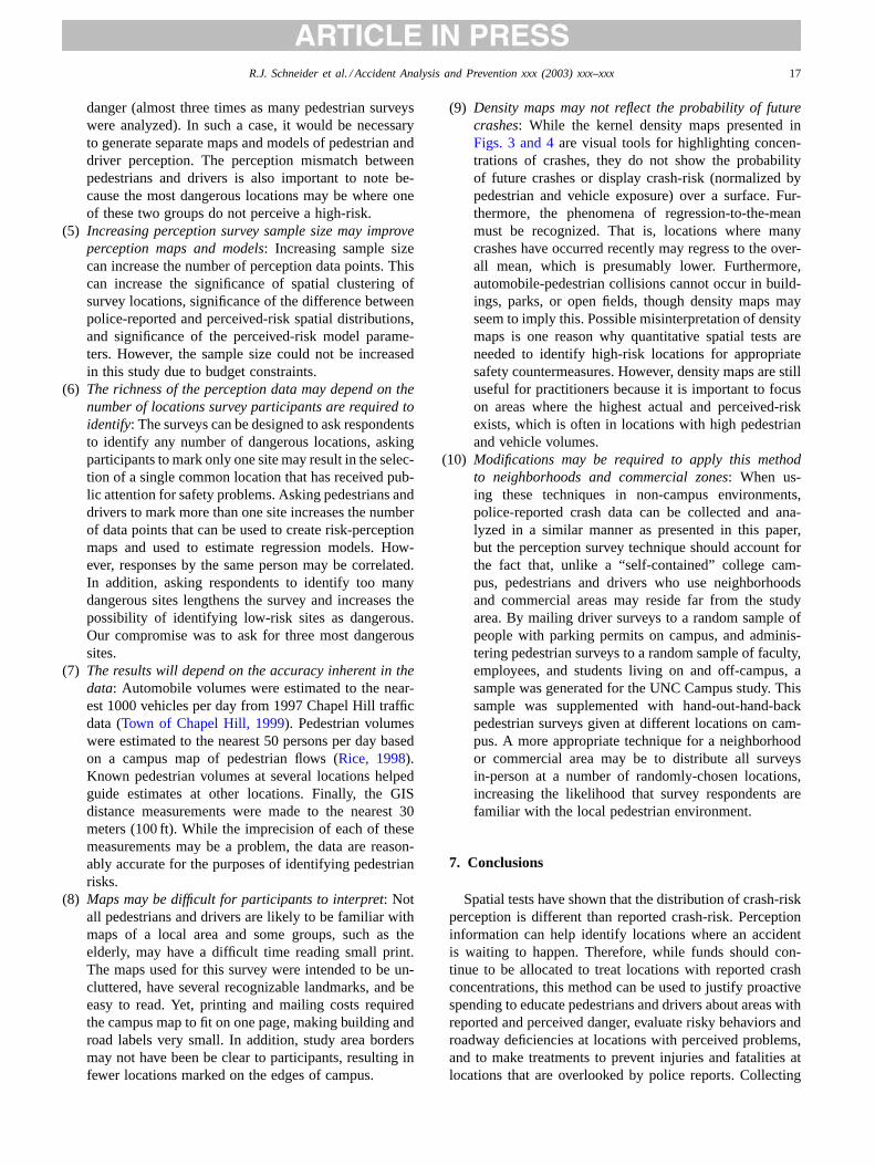
(5) Increasing perception survey sample size may improveperception maps and models: Increasing sample sizecan increase the number of perception data points. Thiscan increase the significance of spatial clustering ofsurvey locations, significance of the difference betweenpolice-reported and perceived-risk spatial distributions,and significance of the perceived-risk model parame-ters. However, the sample size could not be increasedin this study due to budget constraints.

(6) The richness of the perception data may depend on thenumber of locations survey participants are required toidentify: The surveys can be designed to ask respondentsto identify any number of dangerous locations, askingparticipants to mark only one site may result in the selec-tion of a single common location that has received pub-lic attention for safety problems. Asking pedestrians anddrivers to mark more than one site increases the numberof data points that can be used to create risk-perceptionmaps and used to estimate regression models. How-ever, responses by the same person may be correlated.In addition, asking respondents to identify too manydangerous sites lengthens the survey and increases thepossibility of identifying low-risk sites as dangerous.Our compromise was to ask for three most dangeroussites.

(7) The results will depend on the accuracy inherent in thedata: Automobile volumes were estimated to the near-est 1000 vehicles per day from 1997 Chapel Hill trafficdata (Town of Chapel Hill, 1999). Pedestrian volumeswere estimated to the nearest 50 persons per day basedon a campus map of pedestrian flows (Rice, 1998).Known pedestrian volumes at several locations helpedguide estimates at other locations. Finally, the GISdistance measurements were made to the nearest 30meters (100 ft). While the imprecision of each of thesemeasurements may be a problem, the data are reason-ably accurate for the purposes of identifying pedestrianrisks.

(8) Maps may be difficult for participants to interpret: Notall pedestrians and drivers are likely to be familiar withmaps of a local area and some groups, such as theelderly, may have a difficult time reading small print.The maps used for this survey were intended to be un-cluttered, have several recognizable landmarks, and beeasy to read. Yet, printing and mailing costs requiredthe campus map to fit on one page, making building androad labels very small. In addition, study area bordersmay not have been be clear to participants, resulting infewer locations marked on the edges of campus.

(9) Density maps may not reflect the probability of futurecrashes: While the kernel density maps presented inFigs. 3 and 4are visual tools for highlighting concen-trations of crashes, they do not show the probabilityof future crashes or display crash-risk (normalized bypedestrian and vehicle exposure) over a surface. Fur-thermore, the phenomena of regression-to-the-meanmust be recognized. That is, locations where manycrashes have occurred recently may regress to the over-all mean, which is presumably lower. Furthermore,automobile-pedestrian collisions cannot occur in build-ings, parks, or open fields, though density maps mayseem to imply this. Possible misinterpretation of densitymaps is one reason why quantitative spatial tests areneeded to identify high-risk locations for appropriatesafety countermeasures. However, density maps are stilluseful for practitioners because it is important to focuson areas where the highest actual and perceived-riskexists, which is often in locations with high pedestrianand vehicle volumes.

(10) Modifications may be required to apply this methodto neighborhoods and commercial zones: When us-ing these techniques in non-campus environments,police-reported crash data can be collected and ana-lyzed in a similar manner as presented in this paper,but the perception survey technique should account forthe fact that, unlike a “self-contained” college cam-pus, pedestrians and drivers who use neighborhoodsand commercial areas may reside far from the studyarea. By mailing driver surveys to a random sample ofpeople with parking permits on campus, and adminis-tering pedestrian surveys to a random sample of faculty,employees, and students living on and off-campus, asample was generated for the UNC Campus study. Thissample was supplemented with hand-out-hand-backpedestrian surveys given at different locations on cam-pus. A more appropriate technique for a neighborhoodor commercial area may be to distribute all surveysin-person at a number of randomly-chosen locations,increasing the likelihood that survey respondents arefamiliar with the local pedestrian environment.

7. Conclusions

Spatial tests have shown that the distribution of crash-riskperception is different than reported crash-risk. Perceptioninformation can help identify locations where an accidentis waiting to happen. Therefore, while funds should con-tinue to be allocated to treat locations with reported crashconcentrations, this method can be used to justify proactivespending to educate pedestrians and drivers about areas withreported and perceived danger, evaluate risky behaviors androadway deficiencies at locations with perceived problems,and to make treatments to prevent injuries and fatalities atlocations that are overlooked by police reports. Collecting

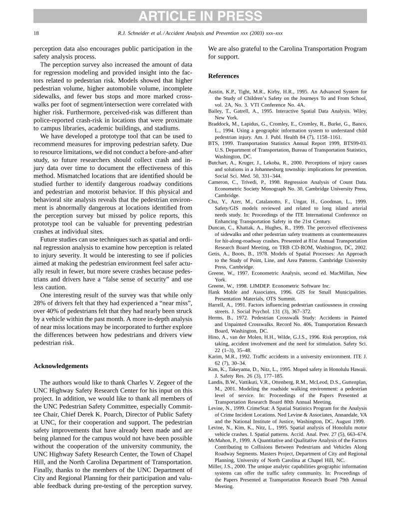
18 R.J. Schneider et al. / Accident Analysis and Prevention xxx (2003) xxx–xxx

perception data also encourages public participation in thesafety analysis process.

The perception survey also increased the amount of datafor regression modeling and provided insight into the fac-tors related to pedestrian risk. Models showed that higherpedestrian volume, higher automobile volume, incompletesidewalks, and fewer bus stops and more marked cross-walks per foot of segment/intersection were correlated withhigher risk. Furthermore, perceived-risk was different thanpolice-reported crash-risk in locations that were proximateto campus libraries, academic buildings, and stadiums.

We have developed a prototype tool that can be used torecommend measures for improving pedestrian safety. Dueto resource limitations, we did not conduct a before-and-afterstudy, so future researchers should collect crash and in-jury data over time to document the effectiveness of thismethod. Mismatched locations that are identified should bestudied further to identify dangerous roadway conditionsand pedestrian and motorist behavior. If this physical andbehavioral site analysis reveals that the pedestrian environ-ment is abnormally dangerous at locations identified fromthe perception survey but missed by police reports, thisprototype tool can be valuable for preventing pedestriancrashes at individual sites.

Future studies can use techniques such as spatial and ordi-nal regression analysis to examine how perception is relatedto injury severity. It would be interesting to see if policiesaimed at making the pedestrian environment feel safer actu-ally result in fewer, but more severe crashes because pedes-trians and drivers have a “false sense of security” and useless caution.

One interesting result of the survey was that while only28% of drivers felt that they had experienced a “near miss”,over 40% of pedestrians felt that they had nearly been struckby a vehicle within the past month. A more in-depth analysisof near miss locations may be incorporated to further explorethe differences between how pedestrians and drivers viewpedestrian risk.

Acknowledgements

The authors would like to thank Charles V. Zegeer of theUNC Highway Safety Research Center for his input on thisproject. In addition, we would like to thank all members ofthe UNC Pedestrian Safety Committee, especially Commit-tee Chair, Chief Derek K. Poarch, Director of Public Safetyat UNC, for their cooperation and support. The pedestriansafety improvements that have already been made and arebeing planned for the campus would not have been possiblewithout the cooperation of the university community, theUNC Highway Safety Research Center, the Town of ChapelHill, and the North Carolina Department of Transportation.Finally, thanks to the members of the UNC Department ofCity and Regional Planning for their participation and valu-able feedback during pre-testing of the perception survey.

We are also grateful to the Carolina Transportation Programfor support.

References

Austin, K.P., Tight, M.R., Kirby, H.R., 1995. An Advanced System forthe Study of Children’s Safety on the Journeys To and From School,vol. 2A, No. 3. VTI Conference No. 4A.

Bailey, T., Gatrell, A., 1995. Interactive Spatial Data Analysis. Wiley,New York.

Braddock, M., Lapidus, G., Cromley, E., Cromley, R., Burke, G., Banco,L., 1994. Using a geographic information system to understand childpedestrian injury. Am. J. Publ. Health 84 (7), 1158–1161.

BTS, 1999. Transportation Statistics Annual Report 1999, BTS99-03.U.S. Department of Transportation, Bureau of Transportation Statistics,Washington, DC.

Butchart, A., Kruger, J., Lekoba, R., 2000. Perceptions of injury causesand solutions in a Johannesburg township: implications for prevention.Social Sci. Med. 50, 331–344.

Cameron, C., Trivedi, P., 1998. Regression Analysis of Count Data.Econometric Society Monograph No. 30, Cambridge University Press,Cambridge.

Chu, Y., Azer, M., Catalanotto, F., Ungar, H., Goodman, L., 1999.Safety/GIS models reviewed and related to long island arterialneeds study. In: Proceedings of the ITE International Conference onEnhancing Transportation Safety in the 21st Century.

Duncan, C., Khattak, A., Hughes, R., 1999. The perceived effectivenessof sidewalks and other pedestrian safety treatments as countermeasuresfor hit-along-roadway crashes. Presented at 81st Annual TransportationResearch Board Meeting, on TRB CD-ROM, Washington, DC, 2002.

Getis, A., Boots, B., 1978. Models of Spatial Processes: An Approachto the Study of Point, Line, and Area Patterns. Cambridge UniversityPress, Cambridge.

Greene, W., 1997. Econometric Analysis, second ed. MacMillan, NewYork.

Greene, W., 1998. LIMDEP. Econometric Software Inc.Hank Mohle and Associates, 1996. GIS for Small Municipalities.

Presentation Materials, OTS Summit.Harrell, A., 1991. Factors influencing pedestrian cautiousness in crossing

streets. J. Social Psychol. 131 (3), 367–372.Herms, B., 1972. Pedestrian Crosswalk Study: Accidents in Painted

and Unpainted Crosswalks. Record No. 406, Transportation ResearchBoard, Washington, DC.

Hino, A., van der Molen, H.H., Wilde, G.J.S., 1996. Risk perception, risktaking, accident involvement and the need for stimulation. Safety Sci.22 (1–3), 35–48.

Karim, M.R., 1992. Traffic accidents in a university environment. ITE J.62 (7), 30–34.

Kim, K., Takeyama, D., Nitz, L., 1995. Moped safety in Honolulu Hawaii.J. Safety Res. 26 (3), 177–185.

Landis, B.W., Vattikuti, V.R., Ottenberg, R.M., McLeod, D.S., Guttenplan,M., 2001. Modeling the roadside walking environment: a pedestrianlevel of service. In: Proceedings of the Papers Presented atTransportation Research Board 80th Annual Meeting.

Levine, N., 1999. CrimeStat: A Spatial Statistics Program for the Analysisof Crime Incident Locations. Ned Levine & Associates, Annandale, VAand the National Institute of Justice, Washington, DC, August 1999.

Levine, N., Kim, K., Nitz, L., 1995. Spatial analysis of Honolulu motorvehicle crashes. I. Spatial patterns. Accid. Anal. Prev. 27 (5), 663–674.

McMahon, P., 1999. A Quantitative and Qualitative Analysis of the FactorsContributing to Collisions Between Pedestrians and Vehicles AlongRoadway Segments. Masters Project, Department of City and RegionalPlanning, University of North Carolina at Chapel Hill, NC.

Miller, J.S., 2000. The unique analytic capabilities geographic informationsystems can offer the traffic safety community. In: Proceedings ofthe Papers Presented at Transportation Research Board 79th AnnualMeeting.

R.J. Schneider et al. / Accident Analysis and Prevention xxx (2003) xxx–xxx 19

Näätänen, R., Summala, H., 1976. Road User Behavior and TrafficAccidents. North-Holland, Amsterdam.

NHTSA, 2000. Traffic Safety Facts 1999, DOT HS 809-093, U.S.Department of Transportation, National Highway Traffic SafetyAdministration (NHTSA), National Center for Statistics and Analysis.Online available from 17 November 2000 at <http://www.nhtsa.dot.gov/people/ncsa>.

North Carolina Center for Geographic Information and Analysis(NCCGIA), 2000. Pedestrian and Bicycle Safety Analysis Tools.

Peled, A., Haj-Yehia, B., Hakkert, A.S., 1996. ArcInfo-Based Geogra-phical Information System for Road Safety Analysis and Improvement.http://www.esri.com/library/userconf/proc96/TO50/PAP005/P5.HTM,accessed on 23 January 2000.

Peterson’s, 2000. Peterson’s Thomson Learning. Peterson’s 4 YearsColleges, Lawrenceville, NJ.

Rice, C.A., 1998. University of North Carolina Estimated Pedestrian FlowsMap. September 1998.

Schneider, R.J., Khattak, A.J., Zegeer, C.V., 2001. A proactive method ofimproving pedestrian safety using GIS: example from a college campus.Transportation Research Record, 1773, TRB, National ResearchCouncil, Washington, DC, pp. 97–107.

Summala, H., 1996. Accident risk and driver behaviour. Safety Sci.22 (1–3), 103–117.

Taylor, P., 1977. Quantitative Methods in Geography: An Introduction toSpatial Analysis. Houghton Mifflin Company, Boston.

Town of Chapel Hill, 1999. Chapel Hill traffic and pedestrian levels. Draftof long-range plan. Transportation, Section 6. North Carolina PlanningDepartment, NC.

US Department of Education, 2000. Digest of Educational Statistics, 1999.NCES 2000-031 (by Thomas D. Snyder, Production Manager; CharleneM. Hoffman), National Center for Education Statistics, WashingtonDC.

Ward, N.J., Wilde, G.J.S., 1996. Driver approach behaviour at anunprotected railway crossing before and after enhancement of lateralsight distances: an experimental investigation of a risk perception andbehavioural compensation hypothesis. Safety Sci. 22 (1–3), 63–75.

Wilde, G.J.S., 1994. Target Risk: Dealing with the Danger of Death,Disease, and Damage in Everyday Decisions. PDE Publications,Toronto, Ont.

Wilde, G.J.S., Gerszke, D., Paulozza, L., 1998. Risk optimization trainingand transfer. Transport. Res. Part F 1, 77–93.

Zegeer, C.V., Stewart, J.R., Huang, H., 2001. Safety Effects of MarkedVs. Unmarked Crosswalks at Uncontrolled Locations: ExecutiveSummary and Recommended Guidelines, FHWA-RD-01-075. U.S.Department of Transportation, Federal Highway Administration, March2002.