ampl models for “not linear” optimization using linear solvers
TRANSCRIPT

Robert Fourer, AMPL Models for “Not Linear” Optimization Using Linear SolversINFORMS Annual Meeting — November 13-16, 2011 — SessionTC10 1
AMPL Models for “Not Linear” Optimization Using Linear Solvers
Robert Fourer
AMPL Optimization LLCwww.ampl.com — +1 773-336-AMPL
Industrial Eng & Management Sciences, Northwestern Univ
INFORMS Annual MeetingCharlotte, NC — November 13-16, 2011Session TC10, Software Demonstrations

Robert Fourer, AMPL Models for “Not Linear” Optimization Using Linear SolversINFORMS Annual Meeting — November 13-16, 2011 — SessionTC10 2
AMPL Models for Unconventional Optimization Using Conventional Solvers
Robert Fourer
AMPL Optimization LLCwww.ampl.com — +1 773-336-AMPL
Industrial Eng & Management Sciences, Northwestern Univ
INFORMS Annual MeetingCharlotte, NC — November 13-16, 2011Session TC10, Software Demonstrations

Robert Fourer, AMPL Models for “Not Linear” Optimization Using Linear SolversINFORMS Annual Meeting — November 13-16, 2011 — SessionTC10 4
AMPL
Algebraic modeling language: symbolic data
set SHIFTS; # shifts
param Nsched; # number of schedules;set SCHEDS = 1..Nsched; # set of schedules
set SHIFT_LIST {SCHEDS} within SHIFTS;
param rate {SCHEDS} >= 0; # pay ratesparam required {SHIFTS} >= 0; # staffing requirements
param least_assign >= 0; # min workers on any schedule used

Robert Fourer, AMPL Models for “Not Linear” Optimization Using Linear SolversINFORMS Annual Meeting — November 13-16, 2011 — SessionTC10 5
AMPL
Algebraic modeling language: symbolic model
var Work {SCHEDS} >= 0 integer;var Use {SCHEDS} >= 0 binary;
minimize Total_Cost:sum {j in SCHEDS} rate[j] * Work[j];
subject to Shift_Needs {i in SHIFTS}: sum {j in SCHEDS: i in SHIFT_LIST[j]} Work[j] >= required[i];
subject to Least_Use1 {j in SCHEDS}:least_assign * Use[j] <= Work[j];
subject to Least_Use2 {j in SCHEDS}:Work[j] <= (max {i in SHIFT_LIST[j]} required[i]) * Use[j];

Robert Fourer, AMPL Models for “Not Linear” Optimization Using Linear SolversINFORMS Annual Meeting — November 13-16, 2011 — SessionTC10 6
AMPL
Explicit data independent of symbolic model
set SHIFTS := Mon1 Tue1 Wed1 Thu1 Fri1 Sat1Mon2 Tue2 Wed2 Thu2 Fri2 Sat2Mon3 Tue3 Wed3 Thu3 Fri3 ;
param Nsched := 126 ;
set SHIFT_LIST[1] := Mon1 Tue1 Wed1 Thu1 Fri1 ;set SHIFT_LIST[2] := Mon1 Tue1 Wed1 Thu1 Fri2 ;set SHIFT_LIST[3] := Mon1 Tue1 Wed1 Thu1 Fri3 ;set SHIFT_LIST[4] := Mon1 Tue1 Wed1 Thu1 Sat1 ;set SHIFT_LIST[5] := Mon1 Tue1 Wed1 Thu1 Sat2 ; .......
param required := Mon1 100 Mon2 78 Mon3 52 Tue1 100 Tue2 78 Tue3 52Wed1 100 Wed2 78 Wed3 52Thu1 100 Thu2 78 Thu3 52Fri1 100 Fri2 78 Fri3 52Sat1 100 Sat2 78 ;
Robert Fourer, AMPL Models for “Not Linear” Optimization Using Linear SolversINFORMS Annual Meeting — November 13-16, 2011 — SessionTC10 7
AMPL
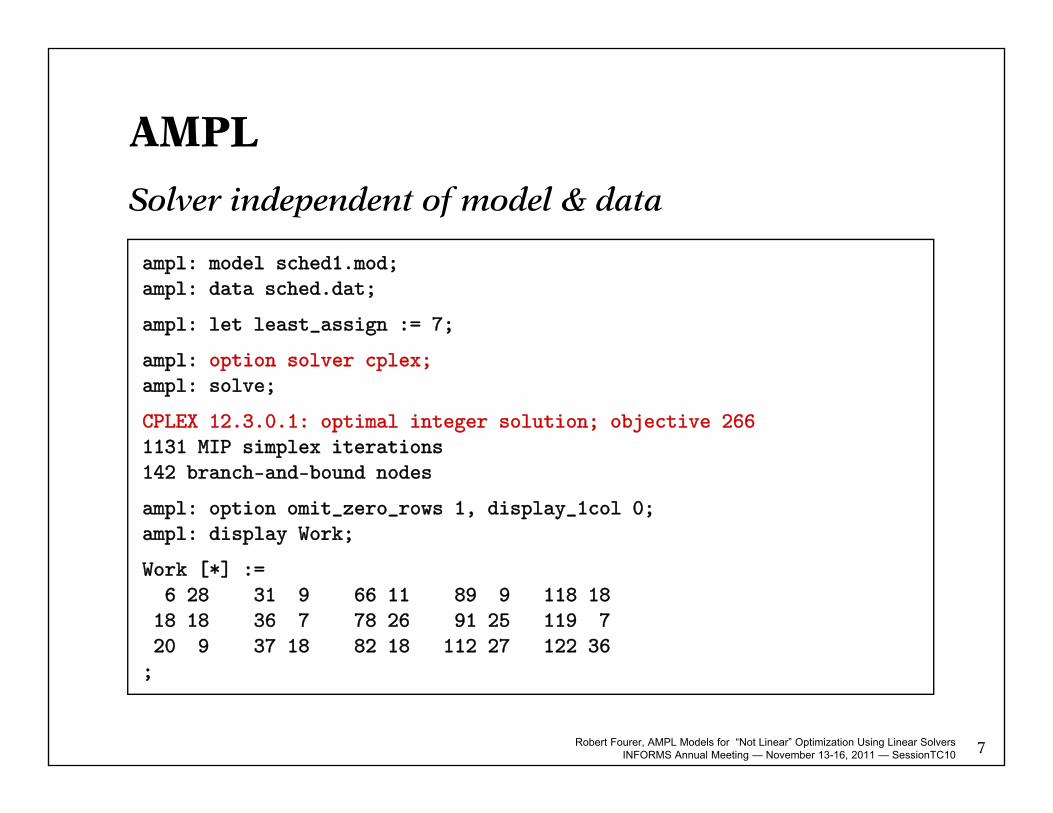
Solver independent of model & data
ampl: model sched1.mod;ampl: data sched.dat;
ampl: let least_assign := 7;
ampl: option solver cplex;ampl: solve;
CPLEX 12.3.0.1: optimal integer solution; objective 2661131 MIP simplex iterations142 branch-and-bound nodes
ampl: option omit_zero_rows 1, display_1col 0;ampl: display Work;
Work [*] :=6 28 31 9 66 11 89 9 118 18
18 18 36 7 78 26 91 25 119 720 9 37 18 82 18 112 27 122 36;

Robert Fourer, AMPL Models for “Not Linear” Optimization Using Linear SolversINFORMS Annual Meeting — November 13-16, 2011 — SessionTC10 8
AMPL
Language independent of solver
ampl: option solver gurobi;ampl: solve;
Gurobi 4.5.0: optimal solution; objective 266504 simplex iterations50 branch-and-cut nodes
ampl: display Work;
Work [*] :=1 20 37 36 89 28 101 12 119 72 8 71 7 91 16 109 28 122 8
21 36 87 7 95 8 116 17 124 28;
Robert Fourer, AMPL Models for “Not Linear” Optimization Using Linear SolversINFORMS Annual Meeting — November 13-16, 2011 — SessionTC10
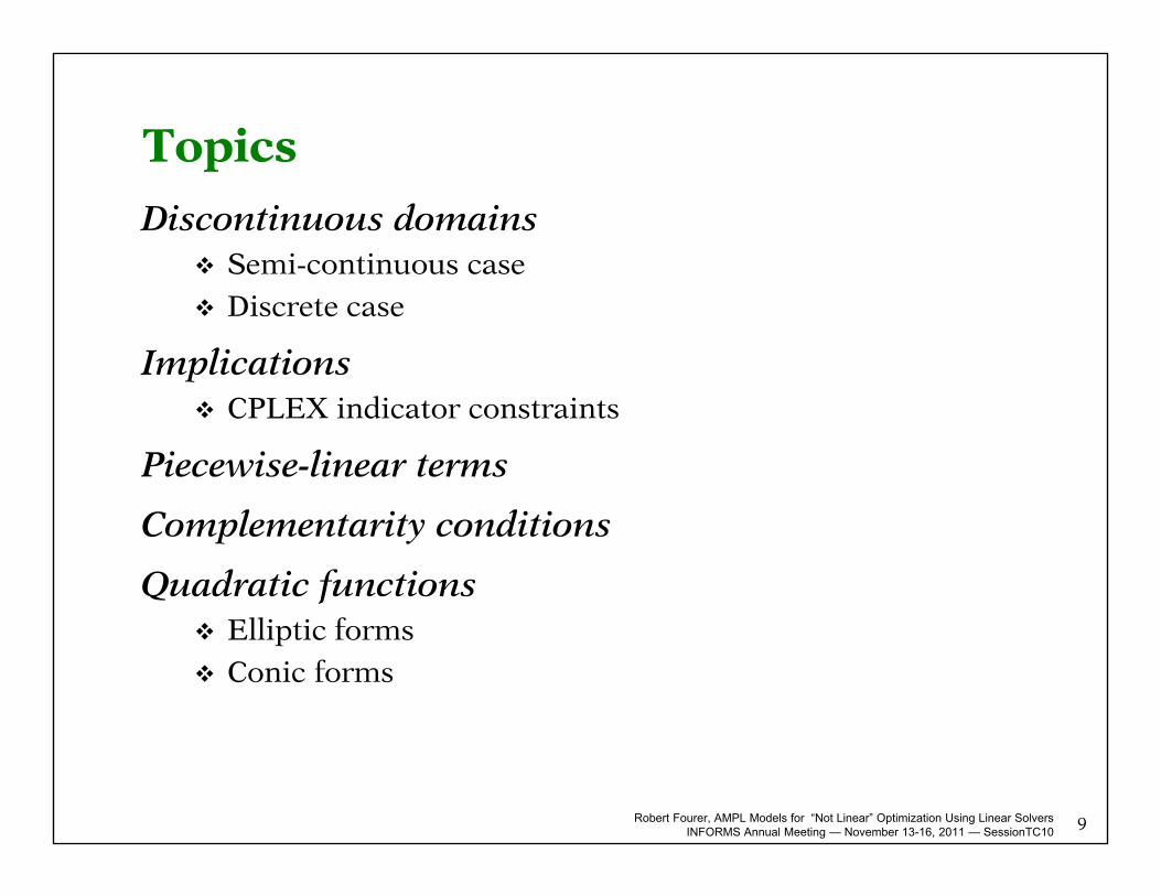
Discontinuous domains Semi-continuous case
Discrete case
Implications CPLEX indicator constraints
Piecewise-linear terms
Complementarity conditions
Quadratic functions Elliptic forms
Conic forms
9
Topics

Robert Fourer, AMPL Models for “Not Linear” Optimization Using Linear SolversINFORMS Annual Meeting — November 13-16, 2011 — SessionTC10
var Work {SCHEDS} >= 0 integer;var Use {SCHEDS} >= 0 binary;
subject to Least_Use1 {j in SCHEDS}:least_assign * Use[j] <= Work[j];
subject to Least_Use2 {j in SCHEDS}:Work[j] <= (max {i in SHIFT_LIST[j]} required[i]) * Use[j];
Formulation with zero-one variables
Discontinuous Domains
var Work {j in SCHEDS} integer, in {0} union
interval [least_assign, (max {i in SHIFT_LIST[j]} required[i])];
Formulation with discrete domains

Robert Fourer, AMPL Models for “Not Linear” Optimization Using Linear SolversINFORMS Annual Meeting — November 13-16, 2011 — SessionTC10 11
Two Common CasesInstead of a continuous variable . . .
var Buy {j in FOOD} >= 0;
Semi-continuous case
var Buy {j in FOOD} in {0} union interval[30,40];
Discrete case
var Buy {j in FOOD} in {1,2,5,10,20,50};
. . . any union of points & intervals possible
Discontinuous Domains

Robert Fourer, AMPL Models for “Not Linear” Optimization Using Linear SolversINFORMS Annual Meeting — November 13-16, 2011 — SessionTC10 12
Semi-Continuous CaseContinuous
CPLEX 12.3.0.1: optimal solution; objective 88.21 dual simplex iterations (0 in phase I)
ampl: display Buy;
BEEF 0 FISH 0 MCH 46.6667 SPG 0CHK 0 HAM 0 MTL 0 TUR 0
Semi-Continuous
CPLEX 12.3.0.1: optimal integer solution; objective 116.4
27 MIP simplex iterations5 branch-and-bound nodes
ampl: display Buy;
BEEF 0 FISH 0 MCH 30 SPG 0CHK 0 HAM 0 MTL 30 TUR 0
Discontinuous Domains

Robert Fourer, AMPL Models for “Not Linear” Optimization Using Linear SolversINFORMS Annual Meeting — November 13-16, 2011 — SessionTC10 13
Semi-Continuous Case (cont’d)Continuous
8 variables, all linear
4 constraints, all linear; 31 nonzeros
1 linear objective; 8 nonzeros.
Semi-Continuous
16 variables:8 binary variables8 linear variables
20 constraints, all linear; 63 nonzeros
1 linear objective; 8 nonzeros.
Discontinuous Domains
Robert Fourer, AMPL Models for “Not Linear” Optimization Using Linear SolversINFORMS Annual Meeting — November 13-16, 2011 — SessionTC10 14
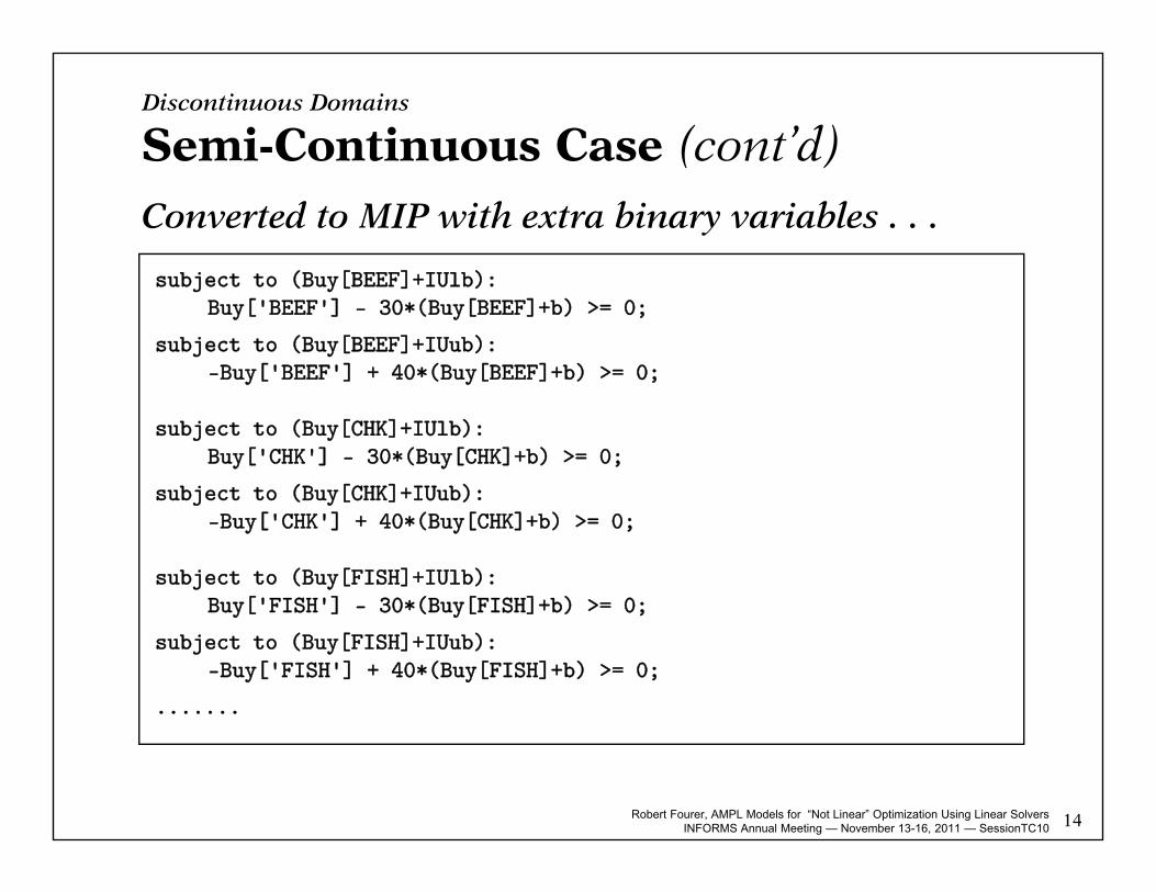
Semi-Continuous Case (cont’d)
Converted to MIP with extra binary variables . . .
subject to (Buy[BEEF]+IUlb):Buy['BEEF'] - 30*(Buy[BEEF]+b) >= 0;
subject to (Buy[BEEF]+IUub):-Buy['BEEF'] + 40*(Buy[BEEF]+b) >= 0;
subject to (Buy[CHK]+IUlb):Buy['CHK'] - 30*(Buy[CHK]+b) >= 0;
subject to (Buy[CHK]+IUub):-Buy['CHK'] + 40*(Buy[CHK]+b) >= 0;
subject to (Buy[FISH]+IUlb):Buy['FISH'] - 30*(Buy[FISH]+b) >= 0;
subject to (Buy[FISH]+IUub):-Buy['FISH'] + 40*(Buy[FISH]+b) >= 0;
.......
Discontinuous Domains

Robert Fourer, AMPL Models for “Not Linear” Optimization Using Linear SolversINFORMS Annual Meeting — November 13-16, 2011 — SessionTC10 15
Discrete CaseContinuous
CPLEX 12.3.0.1: optimal solution; objective 88.21 dual simplex iterations (0 in phase I)
ampl: display Buy;
BEEF 0 FISH 0 MCH 46.6667 SPG 0CHK 0 HAM 0 MTL 0 TUR 0
Discrete
CPLEX 12.3.0.1: optimal integer solution; objective 95.49
51 MIP simplex iterations23 branch-and-bound nodes
ampl: display Buy;
BEEF 1 FISH 1 MCH 10 SPG 5CHK 20 HAM 1 MTL 2 TUR 1
Discontinuous Domains

Robert Fourer, AMPL Models for “Not Linear” Optimization Using Linear SolversINFORMS Annual Meeting — November 13-16, 2011 — SessionTC10 16
Discrete Case (cont’d)
Continuous
8 variables, all linear
4 constraints, all linear; 31 nonzeros
1 linear objective; 8 nonzeros.
Discrete
Substitution eliminates 8 variables.
48 variables, all binary
12 constraints, all linear; 234 nonzeros
1 linear objective; 48 nonzeros.
Discontinuous Domains

Robert Fourer, AMPL Models for “Not Linear” Optimization Using Linear SolversINFORMS Annual Meeting — November 13-16, 2011 — SessionTC10 17
Discrete Case (cont’d)
Converted to MIP in binary variables . . .
minimize Total_Cost:
3.19*(Buy[BEEF]+b)[0] + 6.38*(Buy[BEEF]+b)[1] + 15.95*(Buy[BEEF]+b)[2] + 31.9*(Buy[BEEF]+b)[3] + 63.8*(Buy[BEEF]+b)[4] + 159.5*(Buy[BEEF]+b)[5] + 2.59*(Buy[CHK]+b)[0] + 5.18*(Buy[CHK]+b)[1] + 12.95*(Buy[CHK]+b)[2] + 25.9*(Buy[CHK]+b)[3] + 51.8*(Buy[CHK]+b)[4] + 129.5*(Buy[CHK]+b)[5] + ...
subject to Diet['A']:
700 <= 60*(Buy[BEEF]+b)[0] + 120*(Buy[BEEF]+b)[1] + 300*(Buy[BEEF]+b)[2] + 600*(Buy[BEEF]+b)[3] + 1200*(Buy[BEEF]+b)[4] + 3000*(Buy[BEEF]+b)[5] + 8*(Buy[CHK]+b)[0] + 16*(Buy[CHK]+b)[1] + 40*(Buy[CHK]+b)[2] + 80*(Buy[CHK]+b)[3] + 160*(Buy[CHK]+b)[4] + 400*(Buy[CHK]+b)[5] + ...
Discontinuous Domains

Robert Fourer, AMPL Models for “Not Linear” Optimization Using Linear SolversINFORMS Annual Meeting — November 13-16, 2011 — SessionTC10 18
Discrete Case (cont’d)
and SOS type 1 constraints . . .
subject to (Buy[BEEF]+sos1):
(Buy[BEEF]+b)[0] + (Buy[BEEF]+b)[1] + (Buy[BEEF]+b)[2] + (Buy[BEEF]+b)[3] + (Buy[BEEF]+b)[4] + (Buy[BEEF]+b)[5] = 1;
subject to (Buy[CHK]+sos1):
(Buy[CHK]+b)[0] + (Buy[CHK]+b)[1] + (Buy[CHK]+b)[2] + (Buy[CHK]+b)[3] + (Buy[CHK]+b)[4] + (Buy[CHK]+b)[5] = 1; ...
Discontinuous Domains
Robert Fourer, AMPL Models for “Not Linear” Optimization Using Linear SolversINFORMS Annual Meeting — November 13-16, 2011 — SessionTC10 19
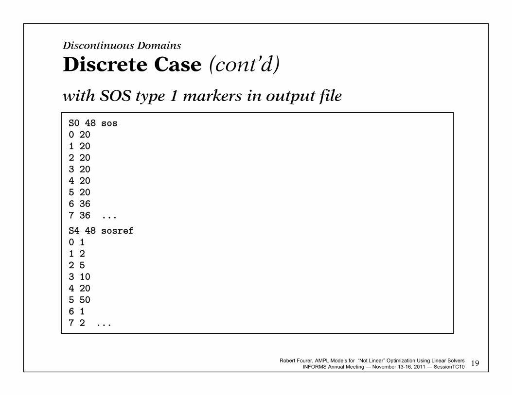
Discrete Case (cont’d)
with SOS type 1 markers in output file
S0 48 sos0 201 202 203 204 205 206 367 36 ...
S4 48 sosref0 11 22 53 104 205 506 17 2 ...
Discontinuous Domains

Robert Fourer, AMPL Models for “Not Linear” Optimization Using Linear SolversINFORMS Annual Meeting — November 13-16, 2011 — SessionTC10
General case Arbitrary union of points and intervals
Auxiliary binary variable for each point or interval
3 auxiliary constraints for each variable
Union of points Auxiliary binary variable for each point
Auxiliary constraint for each variable
Enhanced branching in solver “special ordered sets of type 1”
Zero union interval (semi-continuous) Auxiliary binary variable for each variable
2 auxiliary constraints for each variable
Enhanced branching in solver
20
Conversion for SolverDiscontinuous Domains

Robert Fourer, AMPL Models for “Not Linear” Optimization Using Linear SolversINFORMS Annual Meeting — November 13-16, 2011 — SessionTC10
subject to Least_Use1 {j in SCHEDS}:least_assign * Use[j] <= Work[j];
subject to Least_Use2 {j in SCHEDS}:Work[j] <= (max {i in SHIFT_LIST[j]} required[i]) * Use[j];
Formulation with zero-one variables
Implications
subject to Least_Use1_logical {j in SCHEDS}:Use[j] = 1 ==> Work[j] >= least_assign;
subject to Least_Use2_logical {j in SCHEDS}:Use[j] = 0 ==> Work[j] = 0;
Formulation with implications
subject to Least_Use_logical {j in SCHEDS}:Use[j] = 1 ==> least_assign <= Work[j] else Work[j] = 0;

Robert Fourer, AMPL Models for “Not Linear” Optimization Using Linear SolversINFORMS Annual Meeting — November 13-16, 2011 — SessionTC10
General possibilities Conditional expression
Conditional constraint
Conditional command
AMPL syntax choices if condition then expr1 else expr2
condition ==> constraint1 else constraint2 also <== and <==>
if condition then {commands} else {commands}
Supported by solvers Nonlinear if-then-else
CPLEX indicator constraints
22
Design of Conditional OperatorsImplications

Robert Fourer, AMPL Models for “Not Linear” Optimization Using Linear SolversINFORMS Annual Meeting — November 13-16, 2011 — SessionTC10 23
Nonlinear if-then-elseMore stable expression near zero
subject to logRel {j in 1..N}:
(if X[j] < -delta || X[j] > delta
then log(1+X[j]) / X[j] else (1 - X[j] / 2) <= logLim;
Implications
Robert Fourer, AMPL Models for “Not Linear” Optimization Using Linear SolversINFORMS Annual Meeting — November 13-16, 2011 — SessionTC10
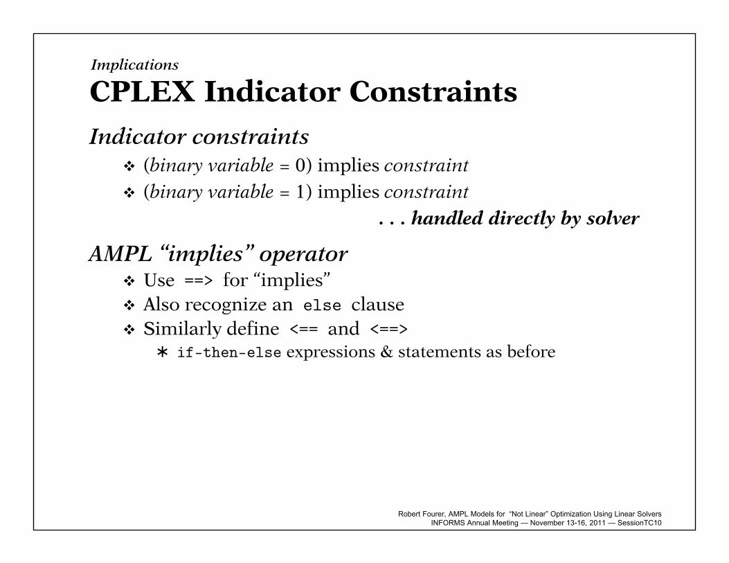
CPLEX Indicator ConstraintsIndicator constraints
(binary variable = 0) implies constraint
(binary variable = 1) implies constraint
. . . handled directly by solver
AMPL “implies” operator Use ==> for “implies” Also recognize an else clause Similarly define <== and <==>
if-then-else expressions & statements as before
Implications

Robert Fourer, AMPL Models for “Not Linear” Optimization Using Linear SolversINFORMS Annual Meeting — November 13-16, 2011 — SessionTC10
Example 1Multicommodity flow with fixed costs
set ORIG; # originsset DEST; # destinationsset PROD; # products
param supply {ORIG,PROD} >= 0; # amounts available at originsparam demand {DEST,PROD} >= 0; # amounts required at destinationsparam limit {ORIG,DEST} >= 0;
param vcost {ORIG,DEST,PROD} >= 0; # variable shipment cost on routesparam fcost {ORIG,DEST} > 0; # fixed cost on routes
var Trans {ORIG,DEST,PROD} >= 0; # actual units to be shippedvar Use {ORIG, DEST} binary; # = 1 iff link is used
minimize total_cost:sum {i in ORIG, j in DEST, p in PROD} vcost[i,j,p] * Trans[i,j,p]
+ sum {i in ORIG, j in DEST} fcost[i,j] * Use[i,j];
Implications

Robert Fourer, AMPL Models for “Not Linear” Optimization Using Linear SolversINFORMS Annual Meeting — November 13-16, 2011 — SessionTC10
Example 1 (cont’d )
Conventional constraints
subject to Supply {i in ORIG, p in PROD}:sum {j in DEST} Trans[i,j,p] = supply[i,p];
subject to Demand {j in DEST, p in PROD}:sum {i in ORIG} Trans[i,j,p] = demand[j,p];
subject to Multi {i in ORIG, j in DEST}:sum {p in PROD} Trans[i,j,p] <= limit[i,j] * Use[i,j];
subject to Supply {i in ORIG, p in PROD}:sum {j in DEST} Trans[i,j,p] = supply[i,p];
subject to Demand {j in DEST, p in PROD}:sum {i in ORIG} Trans[i,j,p] = demand[j,p];
subject to UseDefinition {i in ORIG, j in DEST, p in PROD}:Trans[i,j,p] <= min(supply[i,p], demand[j,p]) * Use[i,j];
Implications

Robert Fourer, AMPL Models for “Not Linear” Optimization Using Linear SolversINFORMS Annual Meeting — November 13-16, 2011 — SessionTC10
Example 1 (cont’d )
Indicator constraint formulations
subject to DefineUsedB {i in ORIG, j in DEST, p in PROD}:
Use[i,j] = 0 ==> Trans[i,j,p] = 0;
subject to DefineUsedC {i in ORIG, j in DEST}:
Use[i,j] = 0 ==> sum {p in PROD} Trans[i,j,p] = 0
else sum {p in PROD} Trans[i,j,p] <= limit[i,j];
subject to DefineUsedA {i in ORIG, j in DEST}:
Use[i,j] = 0 ==> sum {p in PROD} Trans[i,j,p] = 0;
Implications

Robert Fourer, AMPL Models for “Not Linear” Optimization Using Linear SolversINFORMS Annual Meeting — November 13-16, 2011 — SessionTC10
Example 2Assignment to groups with “no one isolated”
var Lone {(i1,i2) in ISO, j in REST} binary;
param give {ISO} default 2;param giveTitle {TITLE} default 2;param giveLoc {LOC} default 2;
param upperbnd {(i1,i2) in ISO, j in REST} :=min (ceil((number2[i1,i2]/card {PEOPLE}) * hiDine[j]) + give[i1,i2],
hiTargetTitle[i1,j] + giveTitle[i1],hiTargetLoc[i2,j] + giveLoc[i2], number2[i1,i2]);
subj to Isolation1 {(i1,i2) in ISO, j in REST}:Assign2[i1,i2,j] <= upperbnd[i1,i2,j] * Lone[i1,i2,j];
subj to Isolation2a {(i1,i2) in ISO, j in REST}:Assign2[i1,i2,j] >= Lone[i1,i2,j];
subj to Isolation2b {(i1,i2) in ISO, j in REST}:Assign2[i1,i2,j] +
sum {ii1 in ADJACENT[i1]: (ii1,i2) in TYPE2} Assign2[ii1,i2,j]>= 2 * Lone[i1,i2,j];
Implications

Robert Fourer, AMPL Models for “Not Linear” Optimization Using Linear SolversINFORMS Annual Meeting — November 13-16, 2011 — SessionTC10
Example 2Same using indicator constraints
var Lone {(i1,i2) in ISO, j in REST} binary;
subj to Isolation1 {(i1,i2) in ISO, j in REST}:Lone[i1,i2,j] = 0 ==> Assign2[i1,i2,j] = 0;
subj to Isolation2b {(i1,i2) in ISO, j in REST}:Lone[i1,i2,j] = 1 ==> Assign2[i1,i2,j] +sum {ii1 in ADJACENT[i1]: (ii1,i2) in TYPE2} Assign2[ii1,i2,j] >= 2;
Implications
Robert Fourer, AMPL Models for “Not Linear” Optimization Using Linear SolversINFORMS Annual Meeting — November 13-16, 2011 — SessionTC10
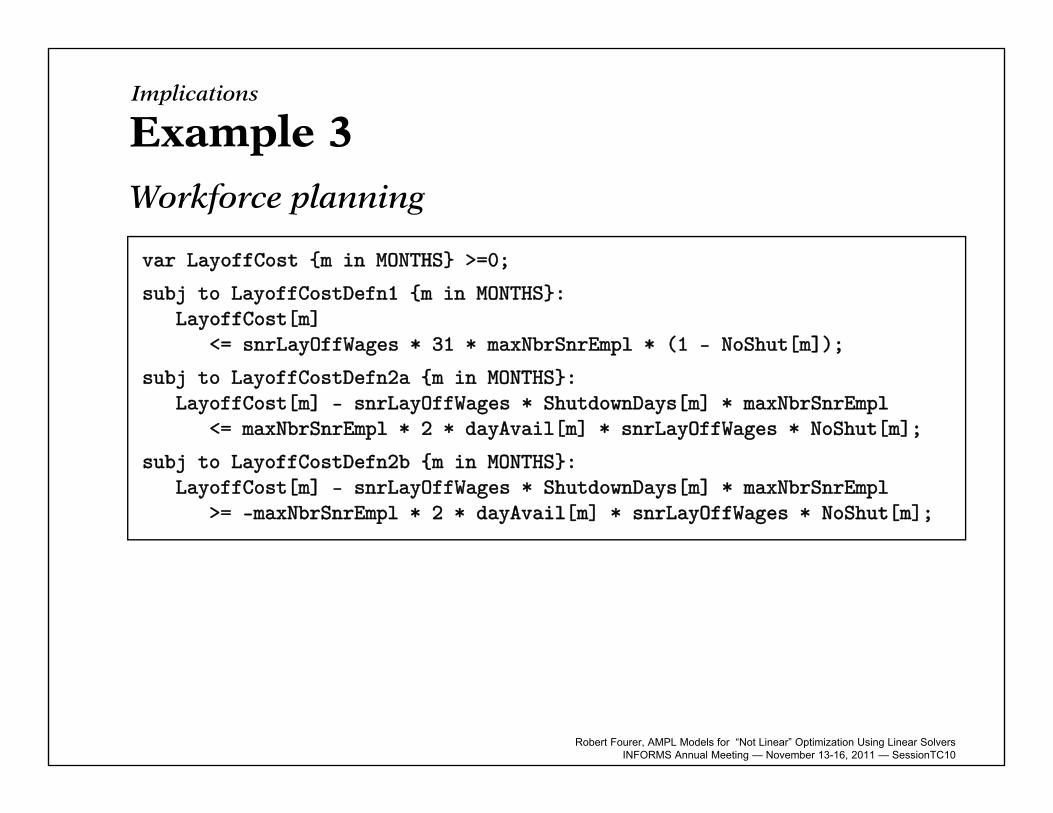
Example 3Workforce planning
var LayoffCost {m in MONTHS} >=0;
subj to LayoffCostDefn1 {m in MONTHS}:LayoffCost[m]
<= snrLayOffWages * 31 * maxNbrSnrEmpl * (1 - NoShut[m]);
subj to LayoffCostDefn2a {m in MONTHS}:LayoffCost[m] - snrLayOffWages * ShutdownDays[m] * maxNbrSnrEmpl
<= maxNbrSnrEmpl * 2 * dayAvail[m] * snrLayOffWages * NoShut[m];
subj to LayoffCostDefn2b {m in MONTHS}:LayoffCost[m] - snrLayOffWages * ShutdownDays[m] * maxNbrSnrEmpl
>= -maxNbrSnrEmpl * 2 * dayAvail[m] * snrLayOffWages * NoShut[m];
Implications

Robert Fourer, AMPL Models for “Not Linear” Optimization Using Linear SolversINFORMS Annual Meeting — November 13-16, 2011 — SessionTC10
Example 3Same using indicator constraints
var LayoffCost {m in MONTHS} >=0;
subj to LayoffCostDefn1 {m in MONTHS}:NoShut[m] = 1 ==> LayoffCost[m] = 0;
subj to LayoffCostDefn2 {m in MONTHS}:NoShut[m] = 0 ==> LayoffCost[m] =
snrLayoffWages * ShutdownDays[m] * maxNumberSnrEmpl;
Implications

Robert Fourer, AMPL Models for “Not Linear” Optimization Using Linear SolversINFORMS Annual Meeting — November 13-16, 2011 — SessionTC10
Conversion for SolverPass logic to CPLEX
AMPL writes “logical” constraints as expression trees AMPL-CPLEX driver “walks” the trees
detects indicator forms converts to CPLEX library calls
CPLEX solves using standard MIP software
Implications
ampl: solve;
252 variables, all nonlinear17 algebraic constraints, all linear; 630 nonzeros
17 inequality constraints126 logical constraints1 linear objective; 2 nonzeros.
CPLEX 12.3.0.1: optimal integer solution; objective 2661265016 MIP simplex iterations231882 branch-and-bound nodes

Robert Fourer, AMPL Models for “Not Linear” Optimization Using Linear SolversINFORMS Annual Meeting — November 13-16, 2011 — SessionTC10
Which is Fastest?Use[j] = 1 ==> least_assign <= Work[j] else Work[j] = 0;
Implications
CPLEX 12.3.0.1: optimal integer solution; objective 2661265016 MIP simplex iterations231882 branch-and-bound nodes
least_assign * Use[j] <= Work[j];Work[j] <= (max {i in SHIFT_LIST[j]} required[i]) * Use[j];
CPLEX 12.3.0.1: optimal integer solution; objective 266776836 MIP simplex iterations109169 branch-and-bound nodes
Use[j] = 1 ==> least_assign <= Work[j] <= (max {i in SHIFT_LIST[j]} required[i]) else Work[j] = 0;
CPLEX 12.3.0.1: optimal integer solution; objective 26613470 MIP simplex iterations2161 branch-and-bound nodes

Robert Fourer, AMPL Models for “Not Linear” Optimization Using Linear SolversINFORMS Annual Meeting — November 13-16, 2011 — SessionTC10
Definition Function of one variable
Linear on intervals
Continuous
Issues Describing the function
choice of specification syntax in the modeling language
Communicating the function to a solver direction description transformation to linear or linear-integer
34
Piecewise-Linear Terms

Robert Fourer, AMPL Models for “Not Linear” Optimization Using Linear SolversINFORMS Annual Meeting — November 13-16, 2011 — SessionTC10
Possibilities List of breakpoints and either:
change in slope at each breakpoint value of the function at each breakpoint
List of slopes and either: distance between breakpoints bounding each slope value of intercept associated with each slope
Lists of breakpoints and slopes
Also needed in some cases One particular breakpoint
One particular slope
Value at one particular point
35
SpecificationPiecewise-Linear

Robert Fourer, AMPL Models for “Not Linear” Optimization Using Linear SolversINFORMS Annual Meeting — November 13-16, 2011 — SessionTC10 36
AMPL Specification: ExamplesPiecewise-Linear
<<0; -1,1>> x[j]
<<-1,1,3,5; -5,-1,0,1.5,3>> x[j]
<<3,5; 0.25,1.00,0.50>> x[j]

Robert Fourer, AMPL Models for “Not Linear” Optimization Using Linear SolversINFORMS Annual Meeting — November 13-16, 2011 — SessionTC10
General forms <breakpoint-list; slope-list> variable
Zero at zero Bounds on variable specified independently
<breakpoint-list; slope-list> (variable, zero-point) Zero at zero-point
<breakpoint-list; slope-list> variable + constant Has value constant at zero
Breakpoint & slope list forms Simple list
<<lim1[i,j],lim2[i,j]; r1[i,j],r2[i,j],r3[i,j]>>
Indexed list << {k in 1..nlim[i,j]} lim[i,j,k];
{k in 1..nlim[i,j]+1} r[i,j,k]>>
37
AMPL Specification: SyntaxPiecewise-Linear

Robert Fourer, AMPL Models for “Not Linear” Optimization Using Linear SolversINFORMS Annual Meeting — November 13-16, 2011 — SessionTC10 38
AMPL Applications (1)Design of a planar structure
var Force {bars}; # Forces on bars:# positive in tension, negative in compression
minimize TotalWeight: (density / yield_stress) *
sum {(i,j) in bars} length[i,j] * <<0; -1,+1>> Force[i,j];
# Weight is proportional to length# times absolute value of force
subject to Xbal {k in joints: k <> fixed}:
sum {(i,k) in bars} xcos[i,k] * Force[i,k]- sum {(k,j) in bars} xcos[k,j] * Force[k,j] = xload[k];
subject to Ybal {k in joints: k <> fixed and k <> rolling}:
sum {(i,k) in bars} ycos[i,k] * Force[i,k]- sum {(k,j) in bars} ycos[k,j] * Force[k,j] = yload[k];
# Forces balance in# horizontal and vertical directions
Piecewise-Linear

Robert Fourer, AMPL Models for “Not Linear” Optimization Using Linear SolversINFORMS Annual Meeting — November 13-16, 2011 — SessionTC10 39
AMPL Applications (2)Data fitting for credit scoring
var Wt_const; # Constant term in computing all scores
var Wt {j in factors} >= if wttyp[j] = 'pos' then 0 else -Infinity<= if wttyp[j] = 'neg' then 0 else +Infinity;
# Weights on the factors
var Sc {i in people}; # Scores for the individuals
minimize Penalty: # Sum of penalties for all individuals
Gratio * sum {i in Good} << {k in 1..Gpce-1} if Gbktyp[k] = 'A'
then Gbkfac[k]*app_amt else Gbkfac[k]*bal_amt[i];
{k in 1..Gpce} Gslope[k] >> Sc[i] +
Bratio * sum {i in Bad} << {k in 1..Bpce-1} if Bbktyp[k] = 'A'
then Bbkfac[k]*app_amtelse Bbkfac[k]*bal_amt[i];
{k in 1..Bpce} Bslope[k] >> Sc[i];
Piecewise-Linear
Robert Fourer, AMPL Models for “Not Linear” Optimization Using Linear SolversINFORMS Annual Meeting — November 13-16, 2011 — SessionTC10 40
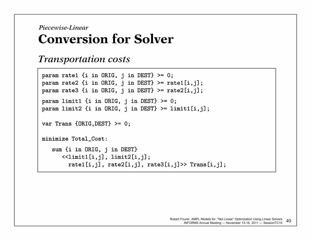
Conversion for Solver
Transportation costs
param rate1 {i in ORIG, j in DEST} >= 0;param rate2 {i in ORIG, j in DEST} >= rate1[i,j];param rate3 {i in ORIG, j in DEST} >= rate2[i,j];
param limit1 {i in ORIG, j in DEST} >= 0;param limit2 {i in ORIG, j in DEST} >= limit1[i,j];
var Trans {ORIG,DEST} >= 0;
minimize Total_Cost:
sum {i in ORIG, j in DEST} <<limit1[i,j], limit2[i,j]; rate1[i,j], rate2[i,j], rate3[i,j]>> Trans[i,j];
Piecewise-Linear

Robert Fourer, AMPL Models for “Not Linear” Optimization Using Linear SolversINFORMS Annual Meeting — November 13-16, 2011 — SessionTC10 41
Minimizing Convex CostsEquivalent linear program
ampl: model trpl2.mod; data trpl.dat; solve;
Substitution eliminates 15 variables.21 piecewise-linear terms replaced by 35 variables and 15 constraints.
Adjusted problem:41 variables, all linear10 constraints, all linear; 82 nonzeros1 linear objective; 41 nonzeros.
CPLEX 10.1.0: optimal solution; objective 19910012 dual simplex iterations (0 in phase I)
ampl: display Trans;
: DET FRA FRE LAF LAN STL WIN :=
CLEV 500 0 200 500 500 500 400GARY 0 0 900 300 0 200 0PITT 700 900 0 200 100 1000 0 ;
Piecewise-Linear
Robert Fourer, AMPL Models for “Not Linear” Optimization Using Linear SolversINFORMS Annual Meeting — November 13-16, 2011 — SessionTC10 42
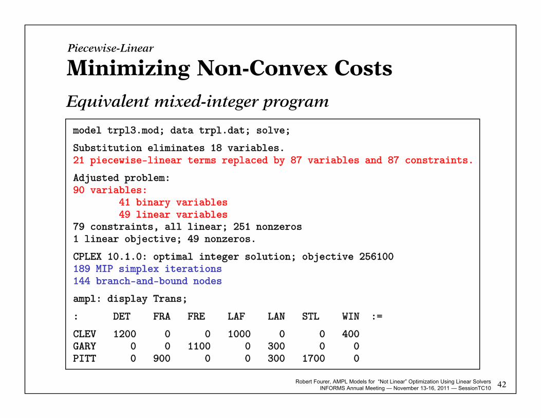
Minimizing Non-Convex CostsEquivalent mixed-integer program
model trpl3.mod; data trpl.dat; solve;
Substitution eliminates 18 variables.21 piecewise-linear terms replaced by 87 variables and 87 constraints.
Adjusted problem:90 variables:
41 binary variables49 linear variables
79 constraints, all linear; 251 nonzeros1 linear objective; 49 nonzeros.
CPLEX 10.1.0: optimal integer solution; objective 256100189 MIP simplex iterations144 branch-and-bound nodes
ampl: display Trans;
: DET FRA FRE LAF LAN STL WIN :=
CLEV 1200 0 0 1000 0 0 400GARY 0 0 1100 0 300 0 0PITT 0 900 0 0 300 1700 0
Piecewise-Linear
Robert Fourer, AMPL Models for “Not Linear” Optimization Using Linear SolversINFORMS Annual Meeting — November 13-16, 2011 — SessionTC10 43
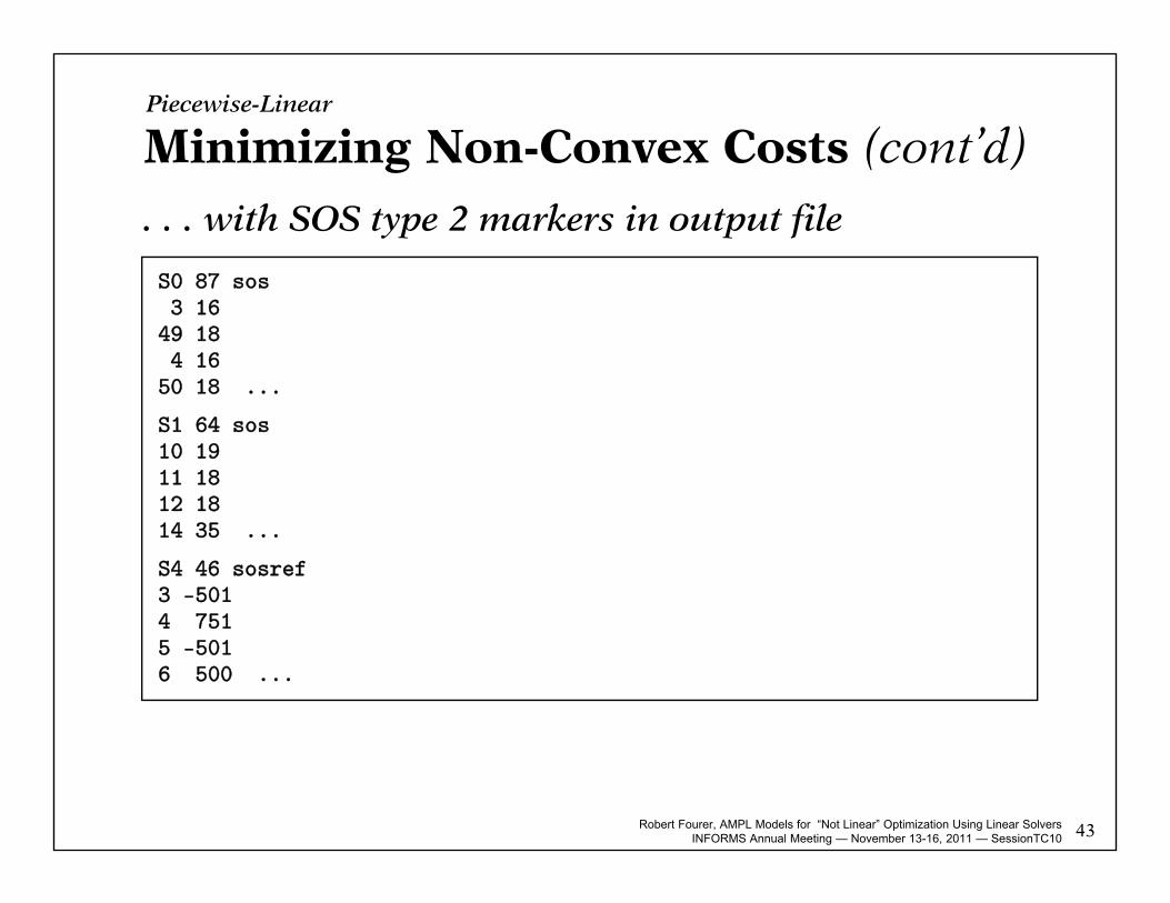
Minimizing Non-Convex Costs (cont’d)
. . . with SOS type 2 markers in output file
S0 87 sos3 1649 184 1650 18 ...
S1 64 sos10 1911 1812 1814 35 ...
S4 46 sosref3 -5014 7515 -5016 500 ...
Piecewise-Linear

Robert Fourer, AMPL Models for “Not Linear” Optimization Using Linear SolversINFORMS Annual Meeting — November 13-16, 2011 — SessionTC10
Equivalent linear program if . . . Objective
minimizes convex (increasing slopes) or maximizes concave (decreasing slopes)
Constraints expressions convex and on the left-hand side of a ≤ constraint convex and on the right-hand side of a ≥ constraint concave and on the left-hand side of a ≥ constraint concave and on the right-hand side of a ≤ constraint
Equivalent mixed-integer program otherwise At least one binary variable per piece
Enhanced branching in solver “special ordered sets of type 2”
44
Conversion for SolverPiecewise-Linear

Robert Fourer, AMPL Models for “Not Linear” Optimization Using Linear SolversINFORMS Annual Meeting — November 13-16, 2011 — SessionTC10
Closely associated with optimization Two inequalities must both hold
At least one must hold with equality
Now can be readily solved Send to standard solver like KNITRO
Let solver reformulate for tractability
45
Complementarity Conditions

Robert Fourer, AMPL Models for “Not Linear” Optimization Using Linear SolversINFORMS Annual Meeting — November 13-16, 2011 — SessionTC10
Elliptic functions
Conic functions
61
Quadratic Functions

Robert Fourer, AMPL Models for “Not Linear” Optimization Using Linear SolversINFORMS Annual Meeting — November 13-16, 2011 — SessionTC10 62
Elliptic Quadratic: ExamplePortfolio optimization
set A; # asset categoriesset T := {1973..1994}; # years
param R {T,A}; # returns on asset categoriesparam mu default 2; # weight on variance
param mean {j in A} = (sum {i in T} R[i,j]) / card(T);
param Rtilde {i in T, j in A} = R[i,j] - mean[j];
var Frac {A} >=0;
var Mean = sum {j in A} mean[j] * Frac[j];
var Variance = sum {i in T} (sum {j in A} Rtilde[i,j]*Frac[j])^2 / card{T};
minimize RiskReward: mu * Variance - Mean;
subject to TotalOne: sum {j in A} Frac[j] = 1;

Robert Fourer, AMPL Models for “Not Linear” Optimization Using Linear SolversINFORMS Annual Meeting — November 13-16, 2011 — SessionTC10 63
Example (cont’d)
Portfolio data
set A := US_3-MONTH_T-BILLS US_GOVN_LONG_BONDS SP_500 WILSHIRE_5000NASDAQ_COMPOSITE LEHMAN_BROTHERS_CORPORATE_BONDS_INDEX EAFE GOLD;
param R:US_3-MONTH_T-BILLS US_GOVN_LONG_BONDS SP_500 WILSHIRE_5000 NASDAQ_COMPOSITE LEHMAN_BROTHERS_CORPORATE_BONDS_INDEX EAFE GOLD :=
1973 1.075 0.942 0.852 0.815 0.698 1.023 0.851 1.677 1974 1.084 1.020 0.735 0.716 0.662 1.002 0.768 1.722 1975 1.061 1.056 1.371 1.385 1.318 1.123 1.354 0.760 1976 1.052 1.175 1.236 1.266 1.280 1.156 1.025 0.960 1977 1.055 1.002 0.926 0.974 1.093 1.030 1.181 1.200 1978 1.077 0.982 1.064 1.093 1.146 1.012 1.326 1.295 1979 1.109 0.978 1.184 1.256 1.307 1.023 1.048 2.212 1980 1.127 0.947 1.323 1.337 1.367 1.031 1.226 1.296 1981 1.156 1.003 0.949 0.963 0.990 1.073 0.977 0.688 1982 1.117 1.465 1.215 1.187 1.213 1.311 0.981 1.084 1983 1.092 0.985 1.224 1.235 1.217 1.080 1.237 0.872 1984 1.103 1.159 1.061 1.030 0.903 1.150 1.074 0.825 ...
Elliptic Quadratic

Robert Fourer, AMPL Models for “Not Linear” Optimization Using Linear SolversINFORMS Annual Meeting — November 13-16, 2011 — SessionTC10 64
Example (cont’d)
Solving with CPLEX
ampl: model markowitz.mod;ampl: data markowitz.dat;
ampl: option solver cplexamp;
ampl: solve;
8 variables, all nonlinear1 constraint, all linear; 8 nonzeros1 nonlinear objective; 8 nonzeros.
CPLEX 12.2.0.0: optimal solution; objective -1.09836247112 QP barrier iterations
ampl:
Elliptic Quadratic

Robert Fourer, AMPL Models for “Not Linear” Optimization Using Linear SolversINFORMS Annual Meeting — November 13-16, 2011 — SessionTC10 65
Example (cont’d)
Solving with CPLEX (simplex)
ampl: model markowitz.mod;ampl: data markowitz.dat;
ampl: option solver cplexamp;ampl: option cplex_options 'primalopt';
ampl: solve;
8 variables, all nonlinear1 constraint, all linear; 8 nonzeros1 nonlinear objective; 8 nonzeros.
CPLEX 12.2.0.0: primaloptNo QP presolve or aggregator reductions.
CPLEX 12.2.0.0: optimal solution; objective -1.0983624765 QP simplex iterations (0 in phase I)
ampl:
Elliptic Quadratic

Robert Fourer, AMPL Models for “Not Linear” Optimization Using Linear SolversINFORMS Annual Meeting — November 13-16, 2011 — SessionTC10 66
Example (cont’d)
Optimal portfolio
ampl: option omit_zero_rows 1;
ampl: display Frac;
EAFE 0.216083GOLD 0.185066
LEHMAN_BROTHERS_CORPORATE_BONDS_INDEX 0.397056WILSHIRE_5000 0.201795 ;
ampl: display Mean, Variance;
Mean = 1.11577Variance = 0.00870377
ampl:
Elliptic Quadratic
Robert Fourer, AMPL Models for “Not Linear” Optimization Using Linear SolversINFORMS Annual Meeting — November 13-16, 2011 — SessionTC10 67
Example (cont’d)
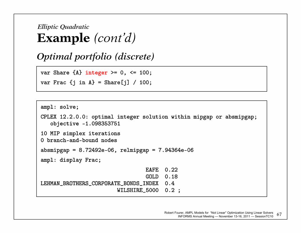
Optimal portfolio (discrete)
var Share {A} integer >= 0, <= 100;
var Frac {j in A} = Share[j] / 100;
Elliptic Quadratic
ampl: solve;
CPLEX 12.2.0.0: optimal integer solution within mipgap or absmipgap; objective -1.098353751
10 MIP simplex iterations0 branch-and-bound nodes
absmipgap = 8.72492e-06, relmipgap = 7.94364e-06
ampl: display Frac;
EAFE 0.22GOLD 0.18
LEHMAN_BROTHERS_CORPORATE_BONDS_INDEX 0.4WILSHIRE_5000 0.2 ;

Robert Fourer, AMPL Models for “Not Linear” Optimization Using Linear SolversINFORMS Annual Meeting — November 13-16, 2011 — SessionTC10
Symbolic detection Objectives
Minimize +. . .+ Minimize ∑ ( + ) , ≥ 0
Constraints +. . . + ≤ ∑ ( + ) ≤ , ≥ 0
Numerical detection Objectives
Minimize + Constraints
+ ≤ . . . where Q is positive semidefinite
68
Detection for SolverElliptic Quadratic

Robert Fourer, AMPL Models for “Not Linear” Optimization Using Linear SolversINFORMS Annual Meeting — November 13-16, 2011 — SessionTC10
Representation Much like LP
Coefficient lists for linear terms Coefficient lists for quadratic terms
A lot simpler than general NLP
Optimization Much like LP
Generalizations of barrier methods Generalizations of simplex methods Extensions of mixed-integer branch-and-bound schemes
Simple derivative computations
Less overhead than general-purpose nonlinear solvers. . . actual speedup will vary
69
SolvingElliptic Quadratic

Robert Fourer, AMPL Models for “Not Linear” Optimization Using Linear SolversINFORMS Annual Meeting — November 13-16, 2011 — SessionTC10 73
Conic Quadratic: Example
Traffic network: symbolic data
set INTERS; # intersections (network nodes)
param EN symbolic; # entranceparam EX symbolic; # exit
check {EN,EX} not within INTERS;
set ROADS within {INTERS union {EN}} cross {INTERS union {EX}};
# road links (network arcs)
param base {ROADS} > 0; # base travel timesparam sens {ROADS} > 0; # traffic sensitivitiesparam cap {ROADS} > 0; # capacities
param through > 0; # throughput
Robert Fourer, AMPL Models for “Not Linear” Optimization Using Linear SolversINFORMS Annual Meeting — November 13-16, 2011 — SessionTC10 74
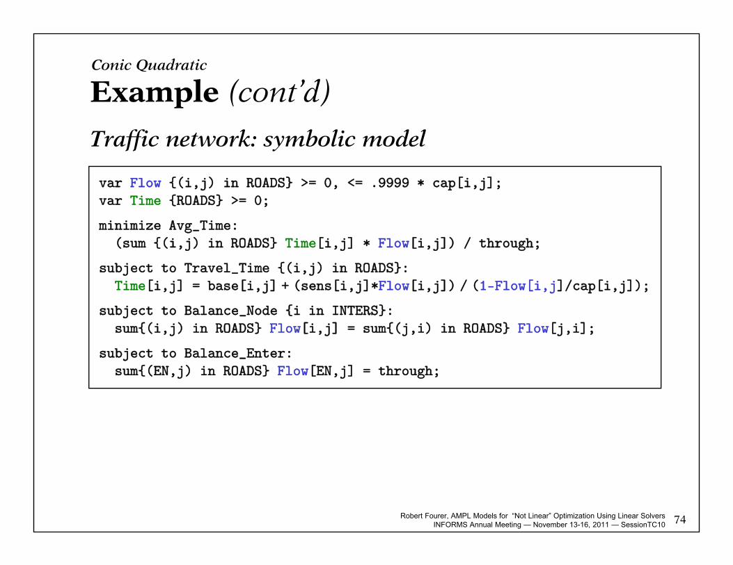
Example (cont’d)
Traffic network: symbolic model
var Flow {(i,j) in ROADS} >= 0, <= .9999 * cap[i,j];var Time {ROADS} >= 0;
minimize Avg_Time:(sum {(i,j) in ROADS} Time[i,j] * Flow[i,j]) / through;
subject to Travel_Time {(i,j) in ROADS}:Time[i,j] = base[i,j] + (sens[i,j]*Flow[i,j]) / (1-Flow[i,j]/cap[i,j]);
subject to Balance_Node {i in INTERS}:sum{(i,j) in ROADS} Flow[i,j] = sum{(j,i) in ROADS} Flow[j,i];
subject to Balance_Enter:sum{(EN,j) in ROADS} Flow[EN,j] = through;
Conic Quadratic

Robert Fourer, AMPL Models for “Not Linear” Optimization Using Linear SolversINFORMS Annual Meeting — November 13-16, 2011 — SessionTC10 75
Example (cont’d)
Traffic network: sample data
set INTERS := b c ;
param EN := a ;param EX := d ;
param: ROADS: base cap sens :=a b 4 10 .1a c 1 12 .7c b 2 20 .9b d 1 15 .5c d 6 10 .1 ;
param through := 20 ;
Conic Quadratic

Robert Fourer, AMPL Models for “Not Linear” Optimization Using Linear SolversINFORMS Annual Meeting — November 13-16, 2011 — SessionTC10 76
Example (cont’d)
Model + data = problem to solve, using KNITRO
ampl: model traffic.mod;ampl: data traffic.dat;
ampl: option solver knitro;ampl: solve;
KNITRO 7.0.0: Locally optimal solution.objective 61.04695019; feasibility error 3.55e-1412 iterations; 25 function evaluations
ampl: display Flow, Time;
: Flow Time :=a b 9.55146 25.2948a c 10.4485 57.5709b d 11.0044 21.6558c b 1.45291 3.41006c d 8.99562 14.9564;
Conic Quadratic

Robert Fourer, AMPL Models for “Not Linear” Optimization Using Linear SolversINFORMS Annual Meeting — November 13-16, 2011 — SessionTC10 77
Example (cont’d)
Same with integer-valued variables
ampl: solve;
KNITRO 7.0.0: Locally optimal solution.objective 76.26375; integrality gap 03 nodes; 5 subproblem solves
ampl: display Flow, Time;
: Flow Time :=a b 9 13a c 11 93.4b d 11 21.625c b 2 4c d 9 15;
var Flow {(i,j) in ROADS} integer >= 0, <= .9999 * cap[i,j];
Conic Quadratic

Robert Fourer, AMPL Models for “Not Linear” Optimization Using Linear SolversINFORMS Annual Meeting — November 13-16, 2011 — SessionTC10 78
Example (cont’d)
Model + data = problem to solve, using CPLEX?
ampl: model traffic.mod;ampl: data traffic.dat;
ampl: option solver cplex;ampl: solve;
CPLEX 12.3.0.0: Constraint _scon[1] is not convex quadratic since it is an equality constraint.
Conic Quadratic

Robert Fourer, AMPL Models for “Not Linear” Optimization Using Linear SolversINFORMS Annual Meeting — November 13-16, 2011 — SessionTC10 79
Example (cont’d)
Look at the model again . . .
var Flow {(i,j) in ROADS} >= 0, <= .9999 * cap[i,j];var Time {ROADS} >= 0;
minimize Avg_Time:(sum {(i,j) in ROADS} Time[i,j] * Flow[i,j]) / through;
subject to Travel_Time {(i,j) in ROADS}:Time[i,j] = base[i,j] + (sens[i,j]*Flow[i,j]) / (1-Flow[i,j]/cap[i,j]);
subject to Balance_Node {i in INTERS}:sum{(i,j) in ROADS} Flow[i,j] = sum{(j,i) in ROADS} Flow[j,i];
subject to Balance_Enter:sum{(EN,j) in ROADS} Flow[EN,j] = through;
Conic Quadratic

Robert Fourer, AMPL Models for “Not Linear” Optimization Using Linear SolversINFORMS Annual Meeting — November 13-16, 2011 — SessionTC10 80
Example (cont’d)
Quadratically constrained reformulation
var Flow {(i,j) in ROADS} >= 0, <= .9999 * cap[i,j];var Delay {ROADS} >= 0;
minimize Avg_Time:sum {(i,j) in ROADS} (base[i,j]*Flow[i,j] + Delay[i,j]) / through;
subject to Delay_Def {(i,j) in ROADS}:sens[i,j] * Flow[i,j]^2 <= (1 - Flow[i,j]/cap[i,j]) * Delay[i,j];
subject to Balance_Node {i in INTERS}:sum{(i,j) in ROADS} Flow[i,j] = sum{(j,i) in ROADS} Flow[j,i];
subject to Balance_Enter:sum{(EN,j) in ROADS} Flow[EN,j] = through;
Conic Quadratic
Robert Fourer, AMPL Models for “Not Linear” Optimization Using Linear SolversINFORMS Annual Meeting — November 13-16, 2011 — SessionTC10 81
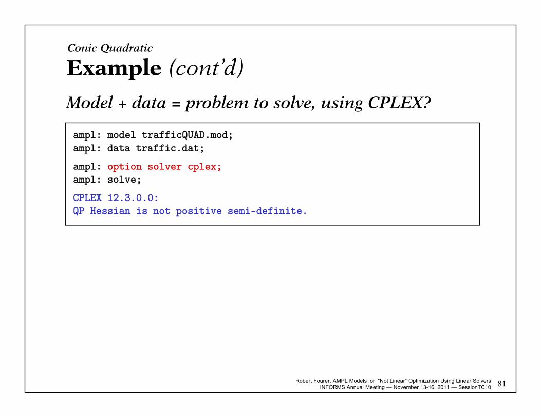
Example (cont’d)
Model + data = problem to solve, using CPLEX?
ampl: model trafficQUAD.mod;ampl: data traffic.dat;
ampl: option solver cplex;ampl: solve;
CPLEX 12.3.0.0: QP Hessian is not positive semi-definite.
Conic Quadratic

Robert Fourer, AMPL Models for “Not Linear” Optimization Using Linear SolversINFORMS Annual Meeting — November 13-16, 2011 — SessionTC10 82
Example (cont’d)
Quadratic reformulation #2
var Flow {(i,j) in ROADS} >= 0, <= .9999 * cap[i,j];var Delay {ROADS} >= 0;var Slack {ROADS} >= 0;
minimize Avg_Time:sum {(i,j) in ROADS} (base[i,j]*Flow[i,j] + Delay[i,j]) / through;
subject to Delay_Def {(i,j) in ROADS}:sens[i,j] * Flow[i,j]^2 <= Slack[i,j] * Delay[i,j];
subject to Slack_Def {(i,j) in ROADS}:Slack[i,j] = 1 - Flow[i,j]/cap[i,j];
subject to Balance_Node {i in INTERS}:sum{(i,j) in ROADS} Flow[i,j] = sum{(j,i) in ROADS} Flow[j,i];
subject to Balance_Enter:sum{(EN,j) in ROADS} Flow[EN,j] = through;
Conic Quadratic

Robert Fourer, AMPL Models for “Not Linear” Optimization Using Linear SolversINFORMS Annual Meeting — November 13-16, 2011 — SessionTC10 83
Example (cont’d)
Model + data = problem to solve, using CPLEX!
ampl: model trafficSOC.mod;ampl: data traffic.dat;
ampl: option solver cplex;ampl: solve;
CPLEX 12.3.0.0: primal optimal; objective 61.0469396815 barrier iterations
ampl: display Flow;
Flow :=a b 9.55175a c 10.4482b d 11.0044c b 1.45264c d 8.99561;
Conic Quadratic

Robert Fourer, AMPL Models for “Not Linear” Optimization Using Linear SolversINFORMS Annual Meeting — November 13-16, 2011 — SessionTC10 84
Example (cont’d)
Same with integer-valued variables
ampl: solve;
CPLEX 12.3.0.0: optimal integer solution within mipgap or absmipgap; objective 76.26375017
19 MIP barrier iterations0 branch-and-bound nodes
ampl: display Flow;
Flow :=a b 9a c 11b d 11c b 2c d 9;
var Flow {(i,j) in ROADS} integer >= 0, <= .9999 * cap[i,j];
Conic Quadratic

Robert Fourer, AMPL Models for “Not Linear” Optimization Using Linear SolversINFORMS Annual Meeting — November 13-16, 2011 — SessionTC10
General nonlinear solver Fewer variables
More natural formulation
MIP solver with convex quadratic option Mathematically simpler formulation
No derivative evaluations no problems with nondifferentiable points
More powerful large-scale solver technologies
85
Which Solver Is Preferable?Conic Quadratic

Robert Fourer, AMPL Models for “Not Linear” Optimization Using Linear SolversINFORMS Annual Meeting — November 13-16, 2011 — SessionTC10
Standard cone
86
Second-Order Cone Programs (SOCPs)
. . . boundary not smooth
Rotated cone ≤ , ≥ 0, ≥ 0, . . .
y
z
+ ≤ ≥ 0 + ≤ , ≥ 0Conic Quadratic
Robert Fourer, AMPL Models for “Not Linear” Optimization Using Linear SolversINFORMS Annual Meeting — November 13-16, 2011 — SessionTC10
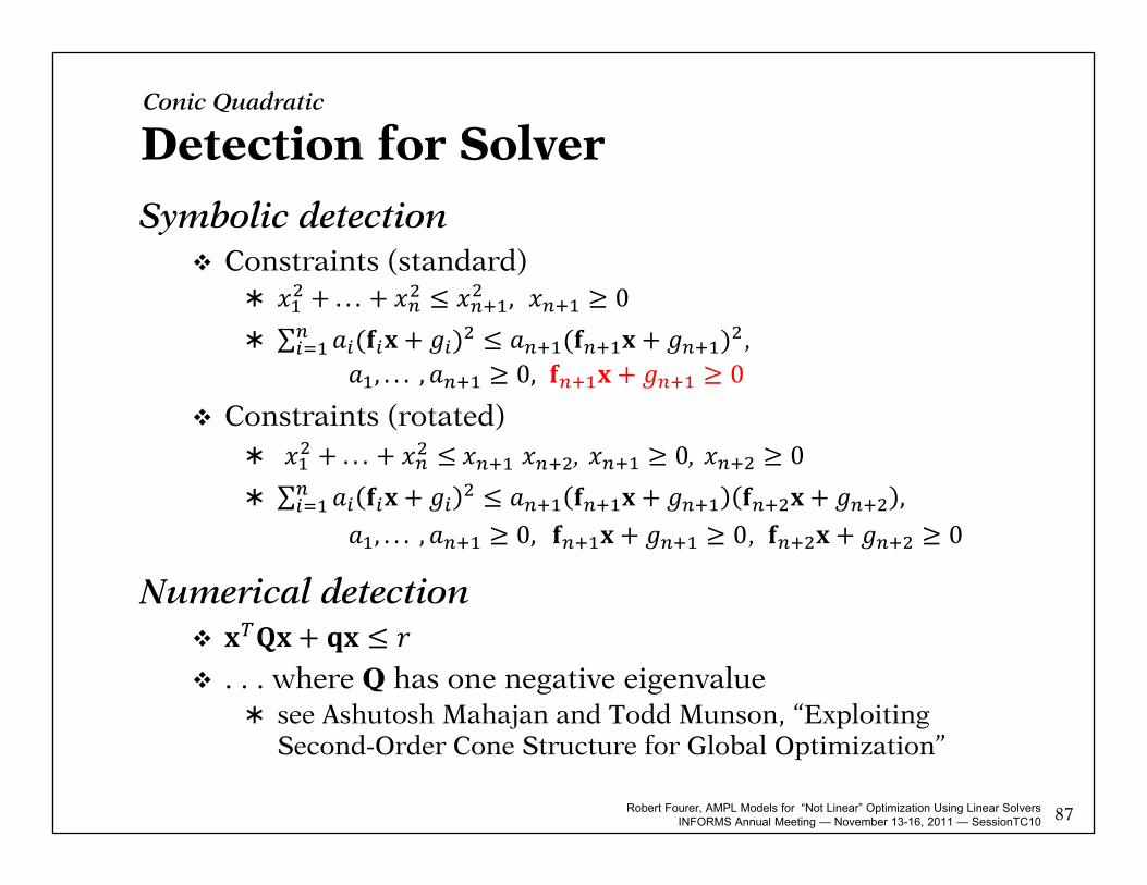
Symbolic detection Constraints (standard)
+. . . + ≤ , ≥ 0 ∑ ( + ) ≤ ( + ) ,, . . . , ≥ 0, + ≥ 0
Constraints (rotated) +. . . + ≤ , ≥ 0, ≥ 0 ∑ + ≤ + + ,, . . . , ≥ 0, + ≥ 0, + ≥ 0
Numerical detection + ≤ . . . where Q has one negative eigenvalue
see Ashutosh Mahajan and Todd Munson, “Exploiting Second-Order Cone Structure for Global Optimization”
87
Detection for SolverConic Quadratic

Robert Fourer, AMPL Models for “Not Linear” Optimization Using Linear SolversINFORMS Annual Meeting — November 13-16, 2011 — SessionTC10
SOC-representable functions Quadratic-linear ratios
Geometric means and generalizations
Norms, p-norms, and generalizations
Available transformations Objectives: Minimize ( ) Constraints: ≤ + , where + ≥ 0 Combinations of these
sums minimums positive multiples
Other objective functions Generalized product-of-powers
Logarithmic Chebychev88
Detection & Conversion for SolverConic Quadratic
Robert Fourer, AMPL Models for “Not Linear” Optimization Using Linear SolversINFORMS Annual Meeting — November 13-16, 2011 — SessionTC10
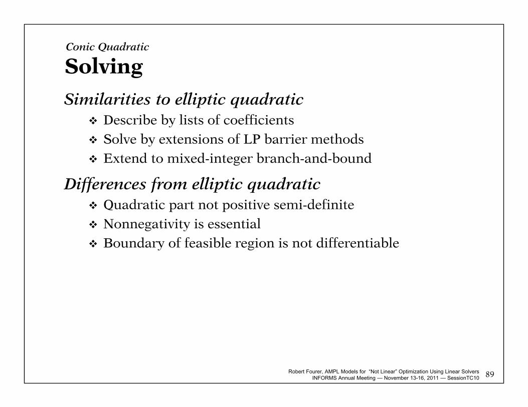
Similarities to elliptic quadratic Describe by lists of coefficients
Solve by extensions of LP barrier methods
Extend to mixed-integer branch-and-bound
Differences from elliptic quadratic Quadratic part not positive semi-definite
Nonnegativity is essential
Boundary of feasible region is not differentiable
89
SolvingConic Quadratic

Robert Fourer, AMPL Models for “Not Linear” Optimization Using Linear SolversINFORMS Annual Meeting — November 13-16, 2011 — SessionTC10
Survey of Test Problems12% of 1238 nonlinear problems were SOC-solvable!
not counting QPs with sum-of-squares objectives
from Vanderbei’s CUTE & non-CUTE, and netlib/ampl
A variety of forms detected hs064 has 4⁄ + 32⁄ + 120⁄ ≤ 1 hs036 minimizes − hs073 has 1.645 0.28 + 0.19 + 20.5 + 0.62 ≤. . . polak4 is a max of sums of squares
hs049 minimizes − + − 1 + − 1 + − 1 emfl_nonconvex has ∑ − ≤
. . . survey of integer programs to come. . . solver tests to come
90
Conic Quadratic