[american institute of aeronautics and astronautics 47th aiaa/asme/asce/ahs/asc structures,...

Path Definitions for Elastically Tailored Conical Shells

Adriana W. Blom∗

Delft University of Technology, Delft, 2629HS, The Netherlands

Brian F. Tatting†

ADOPTECH, Inc., Blacksburg, Virginia, 24060, USA

Jan M.A.M. Hol‡ and Zafer Gurdal§

Delft University of Technology, Delft, 2629HS, The Netherlands

Elastic stiffness tailoring of laminated composite panels by allowing the fibers to curve

within the plane of the laminae has been proven to be beneficial and practical for flat

rectangular plate designs. In this paper the field of application of this variable-stiffness

concept is extended to three-dimensional conical shells with arbitrary dimensions that can

be fabricated using advanced tow-placement machines. The general representation of the

cone geometry is defined to be a function of the two radii and the cone angle. In addition

to cones, the two extreme cases of the cone angle α, namely α = 90◦ and α = 0

◦ yield flat

circular plate and cylinder configurations. Four different path definitions are derived that

describe the variation of the fiber angle along the length of the cone. Manufacturability of

the paths using advanced tow-placement machines has been checked as a function of the

cone geometry and path variables. For those paths that are manufacturable, a complete

ply can be constructed by placing multiple courses on the cone and a complete laminate is

made by stacking multiple plies on top of each other. During this process overlaps or gaps

can occur between the successive passes of the tow-placement machine head, depending

on the cone geometry and fiber angle variation. Tow overlaps may be eliminated by using

the capability to cut and restart the individual tows in the overlap regions so that shells

with uniform thickness are produced. Alternatively, the overlaps may be used to achieve

a grid of integral stiffeners. This paper presents the detailed derivation of the fiber paths

for generalized conical shell surfaces, ranging from annular plates to cylindrical shells.

Different path definitions and resulting laminate geometries are discussed. Implementation

of fabrication details and constraints in terms of the steering radius of curvature and tow

cutting capabilities based on advanced tow-placement technology are demonstrated.

Nomenclature

r Average radius, mw Width of the tow-placement machine, mA Axial length of a cone, mL Longitudinal length along the surface of a cone, ml Arc length, mN Number of coursesn Course identifierp Course width at one side of the central path, mp Perpendicular distance to the central path, mr Radius, m

∗PhD Student, Aerospace Engineering, Delft, Member†Senior Engineer, Blacksburg‡Assistant professor, Aerospace Engineering, Delft§Professor, Aerospace Engineering, Delft, Associate Fellow

1 of 14

American Institute of Aeronautics and Astronautics

47th AIAA/ASME/ASCE/AHS/ASC Structures, Structural Dynamics, and Materials Confere1 - 4 May 2006, Newport, Rhode Island

AIAA 2006-1940

Copyright © 2006 by A.W. Blom. Published by the American Institute of Aeronautics and Astronautics, Inc., with permission.

s Longitudinal surface coordinate, mT User defined fiber orientation angle, radw Course width, mx Longitudinal surface coordinate starting at the small radius, m

Subscripts

0 At the cone end with the small radius1 At the cone end with the large radiuseff Effectiveedge At the edge of a courseorigin At the central path of a coursered Reduced

Conventions

τ Tangent unit vector on the cone surfaceξ In-plane path normal unit vector on the cone surfacea Longitudinal surface unit vectorc Circumferential surface unit vectori Carthesian unit vectorj Carthesian unit vectork Carthesian unit vectorn Surface normal unit vector−→R Vector to an arbitrary point~κ Curvature vector

Symbols

α Cone angle, radβ Angular coordinate on the flattened cone surface, radκ In-plane curvature, m−1

φ Constant fiber orientation angle, radθ Angular coordinate, radϕ Orientation angle of the fiber path, rad

I. Introduction

Traditionally metals have been used as material for aerospace structures. During the last decades othermaterials like fiber reinforced composites and fiber metal laminates started to appear as well, promising

substantial weight savings. Due to the different behavior of these materials new design strategies andproduction methods had to be developed in order to fully exploit their superior properties. Manufacturingof the early applications was mostly done by hand lay-up which introduced many problems: it was notcost competitive, quality of products depended on the craftsman’s skills and therefore the process was notrepeatable. Automated fabrication processes, such as filament winding and tow placement, are a naturalsolution to these problems. They provide repeatable and improved quality production, while reducingproduction cycle time.

Another aspect of the earlier mentioned tow-placement machine is the capability of fabricating tailoredlaminates. Traditionally, unidirectional layers of a composite laminate are placed such that the fibers withinone layer all have the same constant orientation, or have discrete jumps when going from one section toanother. By limiting each ply to a single orientation, the designer is unable to fully utilize the directionalmaterial properties offered by advanced composites for structures that possess stress states that vary as afunction of location within the laminate. Tow-placement machines make it possible to curve the fibers withinthe plane of the laminate, thereby varying the stiffness. This way non-uniform stress states can be accountedfor and even principal load paths can be altered.

Previous research done by Gurdal and Tatting1–3 has focused on applying variable stiffness to flat plateswith central holes, loaded in compression and shear. The results showed that buckling loads could beincreased significantly, ranging from several percent up to a doubling or almost tripling of the buckling load.

2 of 14


Stimulated by these results the next step is to investigate the applicability of variable stiffness for real-life structures, starting by extending the variable-stiffness concept to three-dimensional geometries.4 Inthis paper the definitions for a variable-stiffness cone are derived, while manufacturing limits are takeninto account. Although features like doubly curved surfaces are not present, the first steps are made inunderstanding the difficulties that will be encountered with three-dimensional structures.

II. Fiber Placement Technology

Alaminate constructed by a tow-placement machine is made by having multiple passes of the machine

head following predefined paths. Each path traversed by the tow-placement head which lays down towsis called a course and every arrangement of courses defined to cover a certain area makes up a ply.Although a tow-placement machine can produce much more complex shapes than, for example, a filamentwinding machine, tow placement also has its limitations. If these limitations are already considered in thedesign phase, time will be saved by avoiding unfeasible laminates. Two known limitations of a tow-placementmachine are the minimum turning radius (also called the curvature constraint, where curvature is the inverseof the turning radius) and the minimum cut length.The minimum turning radius of a fiber placement machine is one of the major limitations in producingcurved fiber paths. When fibers are steered, tows at the inner radius might wrinkle if the turning radius istoo small, causing a reduced quality of the laminate. Taking into account the curvature constraint in an earlyphase of defining fiber paths ensures that this limitation will not cause any problems during production.The minimum cut length refers to the minimum length of a tow that can be accurately placed onto a surface.This depends on the distance between the cutting mechanism and the clamps or rollers that hold the towswithin the fiber placement head. When a course is applied to the surface individual tows can be cut andrestarted to adjust the course width locally. If a tow is restarted and cut before the end is adequatelycontrolled, it will not be fed correctly to the compaction roller and hence no accurate placement on the partwill take place.

III. Paths on Conical Shells

In order to make the theory that will be derived as widely applicable as possible, first a general representationof a conical shell will be defined. After that, equations will be derived that define arbitrary fiber paths on

this general cone.

A. Geometry of a Conical shell

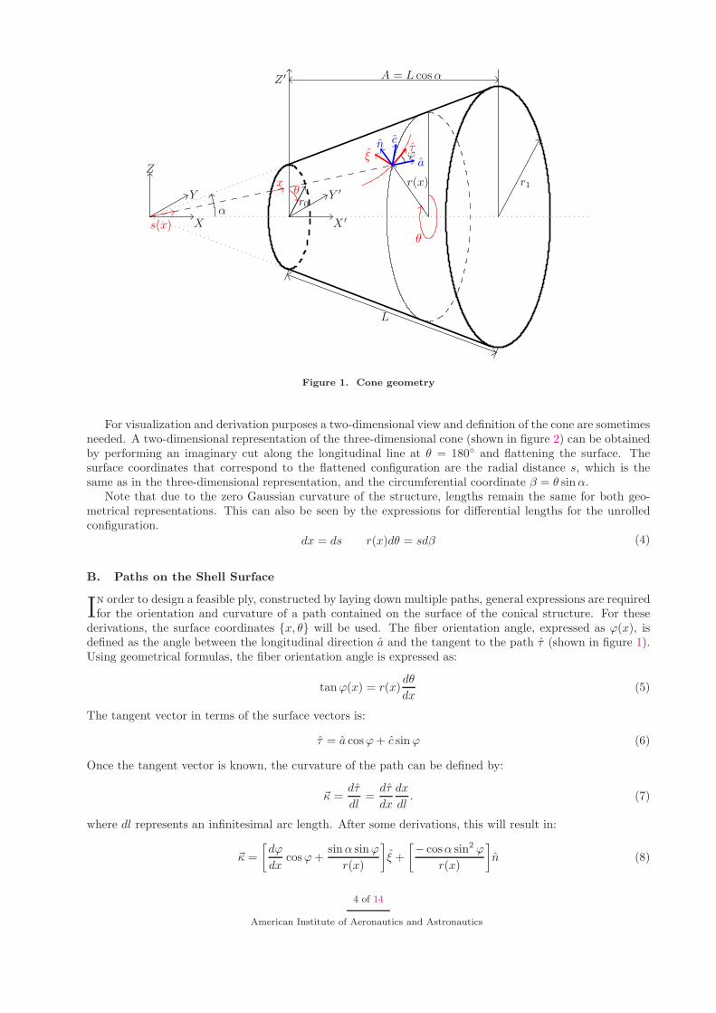
The three-dimensional representation of the geometry of a conical shell is shown in figure 1. The gener-alized coordinates for the thin conical shell are the longitudinal distance x, which runs along the surface

and starts from the small radius of the shell, and the circumferential angle θ, which is measured in theindicated direction with θ = 0 ◦ at the positive Z-axis. The basic parameters to define the shell are the coneangle α and the small and large radii at the two ends r0 and r1, respectively. Alternatively, the axial lengthA or the length along the surface L could be defined, together with the two radii r0 and r1. The cone angleα can then be deduced for further calculations:

tan α =r1 − r0

Aor sin α =

r1 − r0

L(1)

Additionally, the radius r(x) is defined, which is the perpendicular distance from the axis of revolution to apoint on the shell, varying linearly for this conical shell configuration.

r(x) = r0 + x sin α (2)

The conical longitudinal surface coordinate s(x) measures the distance from the cone vertex to a point onthe surface:

s =r(x)

sin α= x +

r0

sinα(3)

Besides the rectangular coordinate system {X, Y, Z} shown in figure 1, the unit vectors for the longitudinaland circumferential surface directions, a and c respectively, as well as the surface normal n will be used.

3 of 14


A = L cosα

ϕ

r1

Z

X

Y

Z ′

X ′

Y ′

x

θ

θr0

r(x)

L

α

a

τcn

ξ

s(x)

Figure 1. Cone geometry

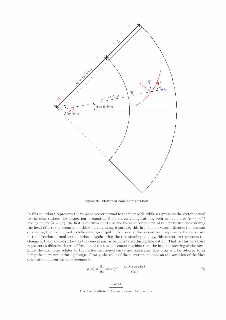
For visualization and derivation purposes a two-dimensional view and definition of the cone are sometimesneeded. A two-dimensional representation of the three-dimensional cone (shown in figure 2) can be obtainedby performing an imaginary cut along the longitudinal line at θ = 180◦ and flattening the surface. Thesurface coordinates that correspond to the flattened configuration are the radial distance s, which is thesame as in the three-dimensional representation, and the circumferential coordinate β = θ sin α.

Note that due to the zero Gaussian curvature of the structure, lengths remain the same for both geo-metrical representations. This can also be seen by the expressions for differential lengths for the unrolledconfiguration.

dx = ds r(x)dθ = sdβ (4)

B. Paths on the Shell Surface

In order to design a feasible ply, constructed by laying down multiple paths, general expressions are requiredfor the orientation and curvature of a path contained on the surface of the conical structure. For these

derivations, the surface coordinates {x, θ} will be used. The fiber orientation angle, expressed as ϕ(x), isdefined as the angle between the longitudinal direction a and the tangent to the path τ (shown in figure 1).Using geometrical formulas, the fiber orientation angle is expressed as:

tan ϕ(x) = r(x)dθ

dx(5)

The tangent vector in terms of the surface vectors is:

τ = a cosϕ + c sin ϕ (6)

Once the tangent vector is known, the curvature of the path can be defined by:

~κ =dτ

dl=

dτ

dx

dx

dl. (7)

where dl represents an infinitesimal arc length. After some derivations, this will result in:

~κ =

[

dϕ

dxcosϕ +

sin α sin ϕ

r(x)

]

ξ +

[

− cosα sin2 ϕ

r(x)

]

n (8)

4 of 14


2π sinα

β = θ sinα

a

cξ τs 0

=r 0/ s

inα

s = r/ sinα

−→R

ϕ

i

j

L

Figure 2. Flattened cone configuration

In this equation ξ represents the in-plane vector normal to the fiber path, while n represents the vector normalto the cone surface. By inspection of equation 8 for known configurations, such as flat plates (α = 90 ◦)and cylinders (α = 0 ◦), the first term turns out to be the in-plane component of the curvature. Envisioningthe head of a tow-placement machine moving along a surface, this in-plane curvature dictates the amountof steering that is required to follow the given path. Conversely, the second term represents the curvaturein the direction normal to the surface. Again using the tow-steering analogy, this curvature represents thechange of the mandrel surface as the conical part is being rotated during fabrication. That is, this curvaturerepresents a different degree of freedom of the tow-placement machine than the in-plane steering of the tows.Since the first term relates to the earlier mentioned curvature constraint, this term will be referred to asbeing the curvature κ during design. Clearly, the value of the curvature depends on the variation of the fiberorientation and on the cone geometry:

κ(x) =dϕ

dxcosϕ(x) +

sin α sin ϕ(x)

r(x)(9)

5 of 14


IV. Ply Construction and Property Tracing

First, general expressions will be derived for constructing a ply and for tracing the properties of anarbitrary point in that ply. Consecutively, these expressions will be used and/or simplified for four

specific course definitions, being a geodesic path, a constant angle path, a path with a linearly varying fiberangle and a path with constant curvature.

A. Constructing a Ply

The first step in constructing a variable-stiffness ply is defining a feasible fiber path, which will be followedby the centerline of the machine head. This fiber path is governed by the fiber orientation angle ϕ(x) and

is defined by the three-dimensional circumferential coordinate θ(x), or alternatively by the two-dimensionalcircumferential coordinate β(s) (shown in figure 2). These are related by:

s = s0 + x

β = θ sin α(10)

A complete ply can be constructed by laying down multiple courses next to each other. Due to the ax-isymmetric nature of the cone, a neighbouring course is found by rotating the original course over an offsetangle, ∆θ. This offset angle depends on the number of courses, N , that is used to build up a ply:

∆θ =2π

N(11)

Alternatively, the offset angle can be expressed in the two-dimensional coordinate ∆β:

∆β = ∆θ sin α =2π sin α

N(12)

In this paper, complete coverage of the cone by one ply is desired, while a minimum number of coursesis used in order to reduce production time. This implies that at every longitudinal location, the numberof courses multiplied by the width of the course in the circumferential direction, called the effective headwidth, weff, should be at least as large as the local circumference. Due to the curved surface and the non-zerofiber orientation, this effective course width differs from the physical width of the course, w. This coursewidth can be equal to the head width of the tow-placement machine w or, if tows are being dropped, smallerthan the machine head width. The analysis needed to find the effective course width will be shown later.The condition for complete coverage is represented by the following equation:

Nweff ≥ 2πr(x) 0 ≤ x ≤ L (13)

The number of courses, which has to be an integer value, is defined by:

N =[

ceil(2πr(x)

weff

)]

max0 ≤ x ≤ L (14)

where the ceil function rounds the real number to the nearest integer towards infinity.For calculation of the effective course width, it is necessary to find the course edges, βleft and βright,

as shown in figure 3. If the course width at one side of the central path is known, the coordinates of thecourse edges can be found by vector analysis. Since the machine head extends perpendicular to the fiberpath, the unit in-plane normal vector ξ (see figure 2) should be multiplied by the course width at one side

of the central path, p (−w

2≤ p ≤

w

2) and added to the vector pointing to the central path. After applying

some transformations, both the vector pointing to an arbitrary point on the course and the normal vectorat that point can be expressed in rectangular coordinates as shown in figure 2:

−→R = s cosβi + s sin βj

ξ = −sin(β + ϕ)i + cos (β + ϕ)j(15)

The edges of a finite head can then be found as:

−→R edge =

[

s cosβ − p sin (β + ϕ)]

i +[

s sin β + p cos (β + ϕ)]

j (16)

6 of 14


{s, β}

{sorigin, βorigin}

{s, βleft}

{s, βright}

p

Left course edge

Course centerline

Right course edge

Figure 3. Course Edges

The corresponding s and β will be:

sedge =√

s2 + p2 − 2ps sinϕ(s) (17)

tan βedge =s sinβ(s) + p cos (β(s) + ϕ(s))

s cosβ(s) − p sin (β(s) + ϕ(s))(18)

In these two equations s and β represent a point on the centerline, which is defined by the path definition.In order to find the effective course width at an arbitrary location s∗, βedge at sedge = s∗ is needed andtherefore s will have to be solved from equation (17). Once s is found, this value will be substituted inequation (18). This way the left and right edges of a course, βleft and βright as shown in figure 3, can be

found as function of s by taking pleft =w

2and pright = −

w

2. The effective course width is related to these

edge coordinates by:weff = s(βleft − βright) (19)

Once this effective course width is calculated for every location along the length of the cone, the minimumnumber of courses can be determined using equation 14.

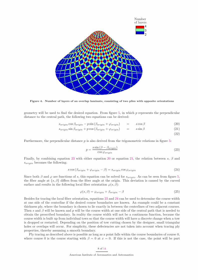
The complete coverage assumption leaves two types of plies that can be constructed: a constant thicknessply and a ply with overlaps. When the course width is kept constant along the path (i.e. no tows are beingdropped), naturally overlaps will occur. By using the tow cutting and restarting capabilities of the tow-placement machine a constant thickness ply can be achieved. In this case, the course width w, or actuallyeven pleft and pright, will be a function of location. Besides the constant thickness ply and the overlap plywhich is made using a constant course width, more control over the overlap is possible by having a coursewidth which is in between the one needed for constant thickness and the maximum course width. An exampleof the thickness buildup for a ±ϕ(x) overlap layer with constant course width is shown in figure 4.

B. Tracing local properties

When a course is laid down, the machine head will be perpendicular to the local fiber orientation.Consequently, every point on a line perpendicular to the fiber direction (e.g. {s, β} in figure 5) will

have the same orientation as the point at the centerline of the machine head ({sorigin, βorigin} in figure 5).The points on the line do not have the same s-coordinate as the center point, though, which implies thatthe fiber angle of a point that does not lie on the centerline deviates from ϕ(s) and needs to be calculated.Therefore, the fiber orientation at any arbitrary point will be a function of both s and β, instead of only afunction of s. In order to find this angle ϕ(s, β), the s-coordinate (= sorigin) that is crossed by the centerof the machine head at the moment that the fiber at {s, β} is laid down, needs to be determined. Simple

7 of 14


Numberof layers

Figure 4. Number of layers of an overlap laminate, consisting of two plies with opposite orientations

geometry will be used to find the desired equation. From figure 5, in which p represents the perpendiculardistance to the central path, the following two equations can be derived:

sorigin cosβorigin − p sin (βorigin + ϕorigin) = s cosβ (20)

sorigin sin βorigin + p cos (βorigin + ϕorigin) = s sin β (21)

(22)

Furthermore, the perpendicular distance p is also derived from the trigonometric relations in figure 5:

p =s sin (β − βorigin)

cosϕorigin

(23)

Finally, by combining equation 23 with either equation 20 or equation 21, the relation between s, β andsorigin becomes the following:

s cos (βorigin + ϕorigin − β) = sorigin cosϕorigin (24)

Since both β and ϕ are functions of s, this equation can be solved for sorigin. As can be seen from figure 5,the fiber angle at {s, β} differs from the fiber angle at the origin. This deviation is caused by the curvedsurface and results in the following local fiber orientation ϕ(s, β):

ϕ(s, β) = ϕorigin + βorigin − β (25)

Besides for tracing the local fiber orientation, equations 23 and 24 can be used to determine the course widthat one side of the centerline if the desired course boundaries are known. An example could be a constantthickness ply, where the boundary is chosen to lie exactly in between the centerlines of two adjacent courses.Then s and β will be known and p will be the course width at one side of the central path that is needed toobtain the prescribed boundary. In reality the course width will not be a continuous function, because thecourse width is built up from individual tows so that the course width will have a discrete change when a towis dropped or restarted. Depending on the position of tow cutting chosen by the designer, small triangularholes or overlaps will occur. For simplicity, these defeciencies are not taken into account when tracing plyproperties, thereby assuming a smooth boundary.

Ply tracing as described above is possible as long as a point falls within the course boundaries of course 0,where course 0 is the course starting with β = 0 at x = 0. If this is not the case, the point will be part

8 of 14


of another course and transformation to course 0 will be necessary. If the courses are numbered such that

course 0 has an initial shift angle β0 = 0 and course n has β0 = n∆β (∆β =2π sin α

N), then the number of

the course in which the point lies can be found by:

n = floor

(

βi − βright(si)

∆β

)

(26)

where the floor function rounds the real number to the nearest integer towards minus infinity. The coursenumber n can be either positive or negative. Due to periodicity every course n is equal to a course n± iN . Apoint on course n can be traced back to a point on course 0 by rotating it, so that βi0 = βred = βi−n∆β. Onceβred is known, the coordinates of the central path can be calculated. After that the local fiber orientationangle ϕ can be calculated as a function of the corresponding s-coordinate of the central path.

βorigin

ϕorigin

ϕorigin

ϕorigin

β − βorigin

ϕ(s, β)

β

{sorigin, βorigin}

{s, β}

p

Course centerline

Arbitrary fiber within a course

Figure 5. Course geometry

For a constant thickness ply each point belongs to a unique course, but in a ply with overlap, an arbitrarypoint could be part of multiple courses and the course numbers of all the courses have to be determined.The order in which courses overlap each other depends on the order in which the courses are being laid downduring manufacturing. Again the first course identifier is found by equation (26), while the presence of anyadditional courses is found by increasing an integer k, starting from 1, such that:

nk+1 = n − k (27)

provided the following condition is fulfilled:

βright ≤ βi − (n − k)∆β ≤ βleft (28)

Once the course numbers are identified, the procedure for finding the fiber angle can be followed for everyindividual layer.Scanning all plies successively and using the order in which the courses are being laid down during manu-facturing, this procedure will provide the local stacking sequence so that the local stiffness matrix can becalculated.

C. Path candidates

Four different path definitions4 are made suitable for use in a design environment. The first is the geodesicpath definition, which is a path laid down on a surface in a natural manner (i.e. no steering required).

The second is a constant angle path, which is useful from an analytical point of view. Third, a linearangle variation is derived, analogous to the definitions used for flat plates1 and finally a path with constantcurvature is defined, which simplifies evaluation of the curvature constraint.

9 of 14


1. Geodesic Path

The first path definition, having zero curvature, is a geodesic path. Because experience in the field ofgeodesic paths is already present, this path definition serves as a basis for other path definitions. Using

the fact that κ = 0, equation 9 can be solved by a change of variables (u(x) = r(x) sin ϕ(x)). Then, bystipulating the fiber angle at the small radius to be T0, the fiber angle variation for a geodesic path will be:

sinϕ =r0 sin T0

r(x)=

s0 sin T0

s(29)

The actual path θ(x) is found by integration of equation 5. Alternatively, this equation can be writtenin the unrolled coordinates (figure 2):

tan ϕ(s) = sdβ

ds(30)

Then the path of the geodesic is defined by:

β(s) = (β0 + T0) − ϕ(s) (31)

where β0 defines the starting position of the path.

2. Constant Angle Path

An alternative to the geodesic path is a constant angle path, which is easy to analyse. The fiber angle isdefined to be:

ϕ(x) = φ (32)

Substituting this in equations 5 and 9, the governing equations for a constant angle path are the following:

dθ

dx=

tan φ

r(x)

κ(x) =sin α sin φ

r(x)

(33)

Looking at this equation it can be noted that the largest value of the curvature occurs at the small radiusof the cone, which makes it easy to determine the feasibility of a path once the geometry is known. Thefunction defining the path will be:

β(s) = tanφ ln

[

s

s0

]

+ β0 or s(β) = s0e

β − β0

tan φ (34)

3. Path with Linearly Varying Fiber Angles

Apath definition that has been used for flat plates is the linearly varying angle path, in which the fiber

angle varies linearly from T0 at the small radius to T1 at the large radius:

ϕ(x) = T0 + (T1 − T0)x

L(35)

The expressions for the three dimensional path definition and the curvature are:

dθ

dx=

tan(

T0 + (T1 − T0)x

L

)

r(x)

κ(x) =T1 − T0

Lcosϕ +

sin α sinϕ

r(x)

(36)

Unfortunately, the path definition can not be written as an explicit function of x and θ, so that the coordinateswill have to be determined numerically by integrating equation 5:

θ(x) =∫ x

0tan

(

T0 + (T1 − T0)x

L

) dx

r(x)

⇒ β(s) =∫ s

s0

tan(

T0 + (T1 − T0)s − s0

L

)ds

s

(37)

Also the minimum curvature will have to be found numerically.

10 of 14


4. Constant Curvature Path

Finally, a path with constant curvature will be defined, so that the curvature constraint can be readilyevaluated. The angle variation will be:

sinϕ(x) =r0 sin T0

r(x)+

κ

sin α

(

r(x)2 − r20

2r(x)

)

=s0 sin T0

s+ κ

(

s2 − s20

2s

)

(38)

If the desired fiber angle at the small radius is set to T0 and the fiber angle at the large radius is set to be T1,the value of the curvature is:

κ =(r1

rsin T1 −

r0

rsin T0

) 1

L

[

r =r0 + r1

2

]

(39)

For the path on the shell surface use is made of the fact that the fiber path is part of a circle. If the2-dimensional angle β as a function of s is desired, the point can be considered to lie on the intersectionof two circles, being the circle that describes the path and the circle with radial coordinate s used for theflattened cylindrical coordinate system.

V. Results

As demonstration for the derived theory, a conical shell with a small radius r0 = 0.125 m, a large radiusr1 = 0.8 m, and a cone angle α = 40 ◦ will serve as a representative cone for a realistic structure.

Furthermore, the specifications of a VIPER advanced tow-placement machine3 developed by CincinattiMilacron will be used. With this machine Gurdal and Tatting produced the variable-stiffness flat testpanels. The limits are based on the use of maximum 24 tows with a tow width of 3.175 mm each (maximumcourse width is 67.2 mm), which has a minimum turning radius ρmin = 0.635m, or equivalently a maximumcurvature κmax = 1.57m−1.

In figure 6(a) three courses with different path definitions are plotted on the three-dimensional conesurface. For each course, the centerline, the left edge and right edge are shown. The displayed constantcurvature path, constant angle path and geodesic path all have the same starting angle T0 = 45 ◦, while theconstant curvature path also has T1 = 45 ◦. Since the constant angle path can be considered to be a specialcase of the linearly varying angle path with T0 = T1, this path can also be seen as a path with T1 = 45 ◦.Although the constant angle and constant curvature path have the same starting and ending angles, thepaths are completely different, as can also be seen in the flattened cone configuration of figure 6(b). Onthe flattened cone the geodesic path is represented by a straight line, which deviates considerably from theother two paths, although this might be expected based on the variation of the fiber orientation as definedin equation 29 and which is plotted in figure 6(c). The fiber orientation of a geodesic path will always goto zero when moving from the small to the large radius of a cone and therefore it will never resemble pathsthat have a (relatively) large angle at the large radius.

The large difference between the constant curvature and constant angle path is caused by the variationof the fiber angle in between the small and large radius, which is also plotted in figure 6(c).

Besides the differences in angle variation, manufacturability of the three paths varies as well. Sincemanufacturability is determined by the maximum curvature of a path, this is an important parameter aswell. The curvature variation of the three paths is plotted in figure 6(d), together with the maximum allowedcurvature. Clearly, the geodesic path can be manufactured, because any geodesic path will always have zerocurvature. Furthermore, the constant curvature path does not violate the maximum curvature constrainteither. Only the constant angle path exceeds the maximum allowed curvature, which means that it cannotbe manufactured using the VIPER tow-placement machine.

11 of 14


Constant curvatureConstant angleGeodesic

(a) Paths on the 3D cone


(b) Paths on the flattened cone


0 0.1 0.2 0.3 0.4 0.5 0.6 0.7 0.8 0.8 1.0

10

20

30

40

50

60

Normalized longitudinal distance, x/L, -

Fib

erangle

,ϕ,deg

(c) Variation of the fiber angle

4 Constant curvatureConstant angleGeodesicMaximum allowed curvature

00 0.1 0.2 0.3 0.4

0.5

0.5 0.6 0.7 0.8 0.8

1.0

1.0

1.5

2.0

2.5

3.0

3.5


Curv

atu

re,κ,m

−1

(d) Variation of the curvature

Figure 6. Different fiber paths with T0 = T1 = 45 ◦

12 of 14


Another example of three courses with varying fiber orientations is shown in figure 7. These paths all havea zero starting angle, while the linearly varying angle path and the constant curvature path have T1 = −70 ◦.As can be seen from figures 7(a) until 7(c), these last two paths are very similar. Again, the major differencebetween the two is the curvature, as is shown in figure 7(d). The constant curvature path just obeys thecurvature constraint, while the linearly varying angle path violates it.

Constant curvatureLinear variationGeodesic

(a) Paths on the 3D cone


(b) Paths on the flattened cone


0

0 0.1 0.2 0.3 0.4 0.5 0.6 0.7 0.8 0.8 1.0

10

-10

-20

-30

-40

-50

-60

-70


Fib

erangle

,ϕ,deg

(c) Variation of the fiber angle

Constant curvatureLinear variationGeodesicMaximum allowed curvature

0

0 0.1

0.2

0.2 0.3

0.4

0.4 0.5

0.6

0.6 0.7

0.8

0.8 0.8

1.0

1.0

1.2

1.4

1.6

1.8

2.0


Curv

atu

re,κ,m

−1

(d) Variation of the curvature

Figure 7. Different fiber paths with T0 = 0 ◦ and T1 = −70 ◦

A more general overview of feasible combinations of T0 and T1 is given in figure 8. In these two figures, acontour plot of the maximum curvature is given as function of the design variables T0 and T1. The feasibledesign space consists of the combinations of T0 and T1 for which the maximum curvature is less than orequal to the tow-placement machine dependent curvature κmax = 1.57m−1.

13 of 14


Fiber orientation angle at the small radius, T0, (deg)

Fib

erori

enta

tion

angle

at

the

larg

era

diu

s,T

1,(d

eg)

-80

-80

-60

-60

-40

-40

-20

-20

20

20

40

40

60

60

80

80

0

00.0

0.5

1.0

1.5

2.0

2.5

3.0

3.5

4.0

4.5

5.0Infeasible design

Infeasible design

(a) Linear angle path definitionFiber orientation angle at the small radius, T0, (deg)

Fib

erori

enta

tion

angle

at

the

larg

era

diu

s,T

1,(d

eg)

-80

-80

-60

-60

-40

-40

-20

-20

20

20

40

40

60

60

80

80

0

00.0

0.5

1.0

1.5

2.0

2.5

3.0

3.5

4.0

4.5

5.0

Infeasible design

Infeasible design

(b) Constant curvature path definition

Figure 8. Maximum curvature, with a marker at the maximum curvature κmax = 1.57m−1

VI. Conclusion

The procedure that is developed for defining fiber paths on a cone with arbitrary dimensions provides afirm basis for constructing stiffness models that take into account varying stiffness in the form of varying

fiber orientation angles and varying thickness. Additionally, the design space for a conical shell with arbitrarydimensions can be determined by calculating the curvature in advance. The developed theory can be usedto generate structural (finite element) analysis models.

References

1Tatting, B. F. and Gurdal, Z., “Design and Manufacture of Elastically Tailored Tow Placed Plates,” Nasa/cr-2002-211919,aug 2002.

2Jegley, D. C., Tatting, B. F., and Gurdal, Z., “Optimization of Elastically Tailored Tow-Placed Plates with Holes,”Proceedings of the 44th AIAA/ASME/ASCE/AHS/ASC Structures, Structural Dynamics and Materials (SDM) Conference,AIAA, apr 2003.

3Tatting, B. F. and Gurdal, Z., “Automated Finite Element Analysis of Elastically-Tailored Plates,” Nasa/cr-2003-212679,dec 2003.

4Blom, A. W., Design of a Variable-Stiffness Cone, Tow Placement Applied to a Section of the Apache Tailboom, Master’sthesis, Delft University of Technology.

14 of 14


[american institute of aeronautics and astronautics 47th aiaa/asme/asce/ahs/asc structures,...

Documents