alternative risk premia: what do we know? - thierry … · alternative risk premia: what do we...

Alternative Risk Premia: What Do We Know?∗

Thierry RoncalliQuantitative Research

Amundi Asset Management, [email protected]

February 2017

Abstract

The concept of alternative risk premia is an extension of the factor investing ap-proach. Factor investing consists in building long-only equity portfolios, which aredirectly exposed to common risk factors like size, value or momentum. Alternative riskpremia designate non-traditional risk premia other than a long exposure to equities andbonds. They may involve equities, rates, credit, currencies or commodities and corre-spond to long/short portfolios. However, contrary to traditional risk premia, it is moredifficult to define alternative risk premia and which risk premia really matter. In fact,the term “alternative risk premia” encompasses two different types of systematic riskfactor: skewness risk premia and market anomalies. For example, the most frequentalternative risk premia are carry and momentum, which are respectively a skewness riskpremium and a market anomaly. Because the returns of alternative risk premia exhibitheterogeneous patterns in terms of statistical properties, option profile and drawdown,asset allocation is more complex than with traditional risk premia. In this context, riskdiversification cannot be reduced to volatility diversification and skewness risk becomesa key component of portfolio optimization. Understanding these different concepts andhow they interconnect is essential for improving multi-asset allocation.

Keywords: Alternative risk premium, factor investing, skewness risk, market anomalies,systematic risk factor, diversification, carry, momentum, value, low beta, short volatility,payoff function, alternative beta, hedge funds, multi-asset allocation.

JEL classification: C50, C60, G11.

1 Introduction

After the emergence of risk-based investing, factor investing has been the new hot topic inthe asset management industry since the 2008 Global Financial Crisis. The two concepts arerelated to the notion of diversification, but take different standpoints. The goal of risk-basedinvesting is to build a better diversified portfolio than a mean-variance optimized portfolio.The idea is that mathematical optimization and volatility minimization do not always leadto financial diversification. The aim of factor investing is to extend the universe of assets forbuilding a diversified allocation by capturing systematic risk factors. For instance, in the

∗This survey has been prepared for the book Factor Investing and Alternative Risk Premia edited byEmmanuel Jurczenko. It is extensively based on my previous three co-authored articles Facts and FantasiesAbout Factor Investing, A Primer on Alternative Risk Premia and Risk Parity Portfolios with SkewnessRisk: An Application to Factor Investing and Alternative Risk Premia. I am profoundly grateful to Em-manuel Jurczenko, Didier Maillard, Bruno Taillardat and Ban Zheng for their helpful comments.

1

Alternative Risk Premia: What Do We Know?

equity space, the capital asset pricing model has been supplemented by a five-factor model,which is based on size, value, momentum, low beta and quality risk factors.

The concept of alternative risk premia (ARP) is an extension of factor investing, whichis a term generally reserved for long-only equity risk factors. Indeed, alternative risk pre-mia concern all the asset classes, not only equities, but also rates, credit, currencies andcommodities. Moreover, they may be implemented using long/short portfolios. To be moreprecise, a risk premium is compensation for taking a risk that cannot be hedged or diver-sified. Traditionally, we consider that there are two main risk premia, which correspond toa long exposure to equities and bonds. However, since the eighties, academics have shownthat there are other sources of risk premia. For instance, cat bonds must incorporate arisk premium, because the investor takes a large risk that cannot be diversified. Therefore,alternative risk premia designate all the risk premia other than a long exposure to equitiesand bonds.

Contrary to traditional risk premia, whose risk/return profile is relatively easy to un-derstand, the behavior of alternative risk premia is more heterogeneous. In fact, they covertwo main categories of strategies: skewness risk premia and market anomalies. Skewnessrisk premia are ‘pure’ risk premia, meaning that they reward systematic risks in bad times.Conversely, market anomalies are strategies that have performed well in the past, but thisperformance cannot be explained by the existence of a risk premium. For example, mo-mentum and trend-following strategies are market anomalies, whereas carry strategies aregenerally considered as skewness risk premia. As a result, statistical properties and optionprofiles are different from one risk premium to another. In particular, skewness risk premiamay exhibit a high skewness risk. Whereas portfolio allocation between traditional risk pre-mia is usually based on expected returns and the covariance matrix, portfolio managementcannot ignore the third statistical moment. This issue is particularly important, becausesome investors see portfolios of alternatives risk premia as all-weather strategies. However,this is not the case in reality.

Diversification is the primary objective when investing in alternative risk premia. Thesecond motivation is the search for higher returns, especially in a low-rate environment. Inthis context, alternative risk premia are performance assets, and not only diversificationassets. It is therefore natural that the development of alternative risk premia impacts thehedge fund industry. First, it offers a new framework for analyzing the risk/return profileof hedge fund strategies and institutional portfolios invested in alternative assets. Second,it provides new investment products that replicate the alternative beta of hedge funds.But the most significant influence of alternative risk premia certainly involves multi-assetmanagement, which cannot be reduced to an allocation between stocks and bonds. Indeed,alternative risk premia constitute the other building blocks of multi-asset portfolios. Thisis why they participate in the convergence of traditional and alternative investments.

This chapter is organized as follows. In section two, we present the rationale of alterna-tive risk premia, in particular the difference between systematic, arbitrage and specific riskfactors. The study of factor investing in the equity market also helps in understanding themotivations behind the emergence of this new framework. In section three, we define moreprecisely the concept of alternative risk premia and make the distinction between skewnessrisk premia and market anomalies. We can then review the different generic strategies. Inparticular, carry and momentum are the two most relevant alternative risk premia acrossthe different asset classes. Section four deals with the issue of diversification and portfoliomanagement in the presence of skewness risk. Finally, section five offers some concludingremarks.

2


2 The rationale of alternative risk premia

In order to understand the relationship between alternative risk premia and the concept ofdiversification, we have to go back to the works of Markowitz (1952) on this topic. In a firststep, we show that diversification depends on the allocation model, but also on the definitionof the common risk factors. In a second step, using the results on the equity asset class, weshow that common risk factors are the only bets that are compatible with diversification.

2.1 Difference between common risk factors and arbitrage factors

We consider a universe of n assets. Let µ and Σ be the vector of expected returns and thecovariance matrix of asset returns. We denote by x = (x1, . . . , xn) the vector of weights in theportfolio. For Markowitz (1952), the financial problem of the investor consists in maximizingthe expected excess return of his portfolio subject to a constraint on the portfolio’s volatility:

x? = arg maxx> (µ− r1)

u.c.√x>Σx ≤ σ? (1)

where r is the return of the risk-free asset. Markowitz (1956) showed that this non-linearoptimization problem is equivalent to a quadratic optimization problem:

x? = arg min1

2x>Σx− γx> (µ− r1) (2)

where γ is a parameter that controls the risk aversion of the investor. Without any con-straints, the mean-variance optimized (MVO) portfolio x? is equal to γΣ−1 (µ− r1). Moregenerally, in the presence of linear equality and inequality constraints, MVO portfolios areof the following form:

x? ∝ f(µ,Σ−1

)(3)

where f is a complicated function that depends on the constraints. More precisely, thesolution of the Markowitz optimization problem depends on the inverse of the covariancematrix and not the covariance matrix itself. Therefore, the important quantity in portfoliooptimization is the information matrix I = Σ−1.

In order to better understand the notion of information matrix, we consider the eigen-decomposition of the covariance matrix Σ:

Σ = V ΛV > (4)

where V is the matrix of eigenvectors of Σ and Λ is the diagonal matrix, whose elementsare the eigenvalues of Σ. We have:

Σ−1 =(V ΛV >

)−1

=(V >)−1

Λ−1V −1

= V Λ−1V > (5)

because V is an orthogonal matrix. It follows that the eigenvectors of the information matrixI are the same as those of the covariance matrix. This is not the case of eigenvalues. Indeed,the eigenvalues of I are the inverse of the eigenvalues of Σ.

3


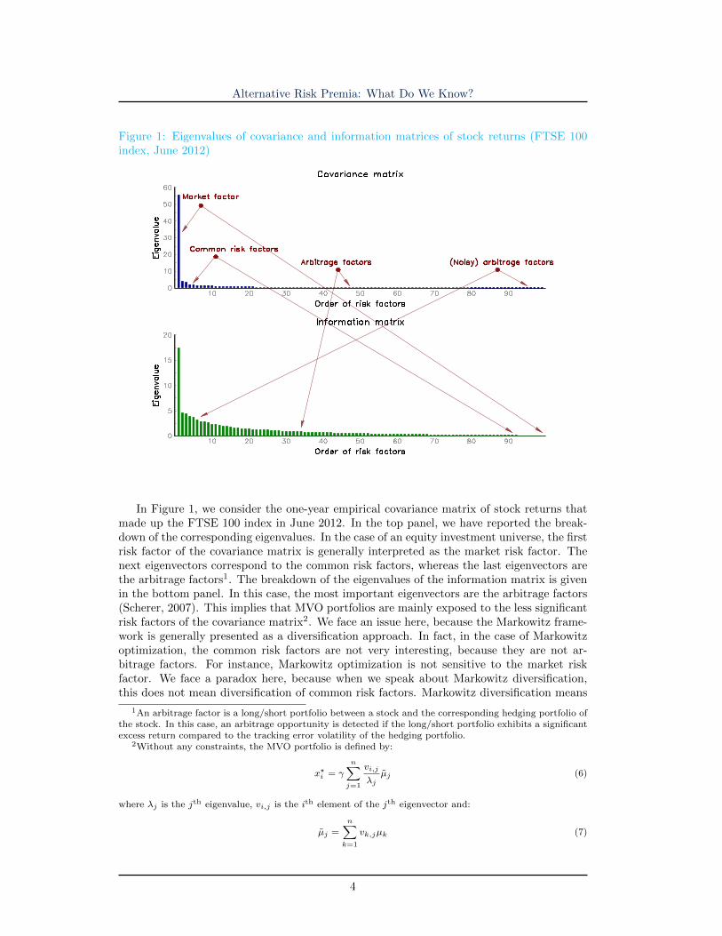
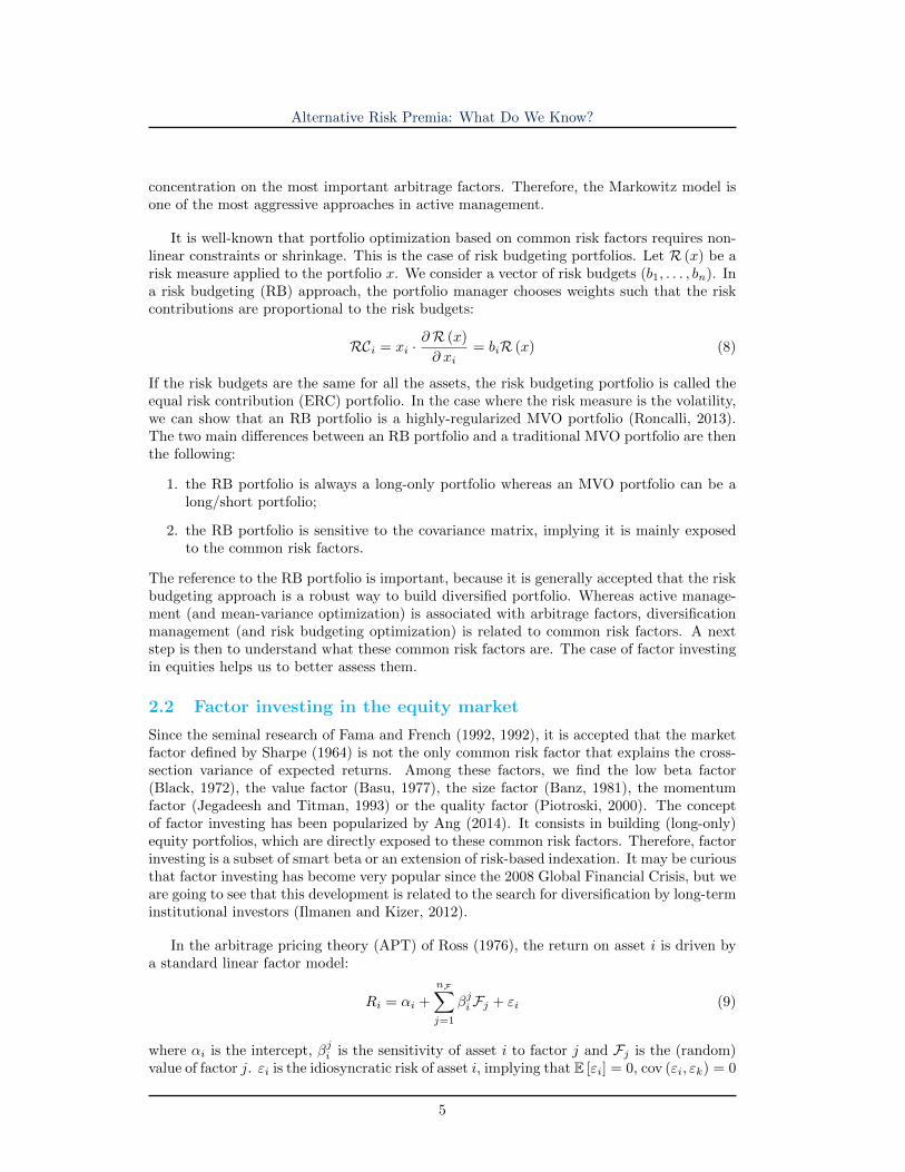
Figure 1: Eigenvalues of covariance and information matrices of stock returns (FTSE 100index, June 2012)

In Figure 1, we consider the one-year empirical covariance matrix of stock returns thatmade up the FTSE 100 index in June 2012. In the top panel, we have reported the break-down of the corresponding eigenvalues. In the case of an equity investment universe, the firstrisk factor of the covariance matrix is generally interpreted as the market risk factor. Thenext eigenvectors correspond to the common risk factors, whereas the last eigenvectors arethe arbitrage factors1. The breakdown of the eigenvalues of the information matrix is givenin the bottom panel. In this case, the most important eigenvectors are the arbitrage factors(Scherer, 2007). This implies that MVO portfolios are mainly exposed to the less significantrisk factors of the covariance matrix2. We face an issue here, because the Markowitz frame-work is generally presented as a diversification approach. In fact, in the case of Markowitzoptimization, the common risk factors are not very interesting, because they are not ar-bitrage factors. For instance, Markowitz optimization is not sensitive to the market riskfactor. We face a paradox here, because when we speak about Markowitz diversification,this does not mean diversification of common risk factors. Markowitz diversification means

1An arbitrage factor is a long/short portfolio between a stock and the corresponding hedging portfolio ofthe stock. In this case, an arbitrage opportunity is detected if the long/short portfolio exhibits a significantexcess return compared to the tracking error volatility of the hedging portfolio.

2Without any constraints, the MVO portfolio is defined by:

x?i = γn∑

j=1

vi,j

λjµj (6)

where λj is the jth eigenvalue, vi,j is the ith element of the jth eigenvector and:

µj =

n∑k=1

vk,jµk (7)

4


concentration on the most important arbitrage factors. Therefore, the Markowitz model isone of the most aggressive approaches in active management.

It is well-known that portfolio optimization based on common risk factors requires non-linear constraints or shrinkage. This is the case of risk budgeting portfolios. Let R (x) be arisk measure applied to the portfolio x. We consider a vector of risk budgets (b1, . . . , bn). Ina risk budgeting (RB) approach, the portfolio manager chooses weights such that the riskcontributions are proportional to the risk budgets:

RCi = xi ·∂R (x)

∂ xi= biR (x) (8)

If the risk budgets are the same for all the assets, the risk budgeting portfolio is called theequal risk contribution (ERC) portfolio. In the case where the risk measure is the volatility,we can show that an RB portfolio is a highly-regularized MVO portfolio (Roncalli, 2013).The two main differences between an RB portfolio and a traditional MVO portfolio are thenthe following:

1. the RB portfolio is always a long-only portfolio whereas an MVO portfolio can be along/short portfolio;

2. the RB portfolio is sensitive to the covariance matrix, implying it is mainly exposedto the common risk factors.

The reference to the RB portfolio is important, because it is generally accepted that the riskbudgeting approach is a robust way to build diversified portfolio. Whereas active manage-ment (and mean-variance optimization) is associated with arbitrage factors, diversificationmanagement (and risk budgeting optimization) is related to common risk factors. A nextstep is then to understand what these common risk factors are. The case of factor investingin equities helps us to better assess them.

2.2 Factor investing in the equity market

Since the seminal research of Fama and French (1992, 1992), it is accepted that the marketfactor defined by Sharpe (1964) is not the only common risk factor that explains the cross-section variance of expected returns. Among these factors, we find the low beta factor(Black, 1972), the value factor (Basu, 1977), the size factor (Banz, 1981), the momentumfactor (Jegadeesh and Titman, 1993) or the quality factor (Piotroski, 2000). The conceptof factor investing has been popularized by Ang (2014). It consists in building (long-only)equity portfolios, which are directly exposed to these common risk factors. Therefore, factorinvesting is a subset of smart beta or an extension of risk-based indexation. It may be curiousthat factor investing has become very popular since the 2008 Global Financial Crisis, but weare going to see that this development is related to the search for diversification by long-terminstitutional investors (Ilmanen and Kizer, 2012).

In the arbitrage pricing theory (APT) of Ross (1976), the return on asset i is driven bya standard linear factor model:

Ri = αi +

nF∑j=1

βjiFj + εi (9)

where αi is the intercept, βji is the sensitivity of asset i to factor j and Fj is the (random)value of factor j. εi is the idiosyncratic risk of asset i, implying that E [εi] = 0, cov (εi, εk) = 0

5


for i 6= k and cov (εi,Fj) = 0. The R-squared coefficient associated with Model (9) is equalto:

R2i = 1− σ2 (εi)

σ2 (Ri)(10)

It measures the part of the variance of asset returns explained by common factors. It followsthat the part due to the idiosyncratic risk is equal to 1−R2

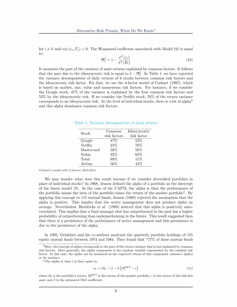
i . In Table 1, we have reportedthe variance decomposition of daily returns of 6 stocks between common risk factors andthe idiosyncratic risk factor. For that, we use the 4-factor model of Carhart (1997), whichis based on market, size, value and momentum risk factors. For instance, if we considerthe Google stock, 47% of the variance is explained by the four common risk factors and53% by the idiosyncratic risk. If we consider the Netflix stock, 76% of the return variancecorresponds to an idiosyncratic risk. At the level of individual stocks, there is a lot of alpha3

and this alpha dominates common risk factors.

Table 1: Variance decomposition of stock returns

StockCommon Idiosyncratic

risk factors risk factorGoogle 47% 53%Netflix 24% 76%Mastercard 50% 50%Nokia 32% 68%Total 89% 11%Airbus 56% 44%

Carhart’s model with 4 factors, 2010-2014.

We may wonder what does this result become if we consider diversified portfolios inplace of individual stocks? In 1968, Jensen defined the alpha of a portfolio as the interceptof the linear model (9). In the case of the CAPM, the alpha is then the performance ofthe portfolio minus the beta of the portfolio times the return of the market portfolio4. Byapplying this concept to 115 mutual funds, Jensen (1968) rejected the assumption that thealpha is positive. This implies that the active management does not produce alpha onaverage. Nevertheless, Hendricks et al. (1993) noticed that this alpha is positively auto-correlated. This implies that a fund manager that has outperformed in the past has a higherprobability of outperforming than underperforming in the future. This result suggested thenthat there is a persistence of the performance of active management and this persistence isdue to the persistence of the alpha.

In 1995, Grinblatt and his co-authors analyzed the quarterly portfolio holdings of 155equity mutual funds between 1974 and 1984. They found that “77% of these mutual funds

3Here, the concept of alpha corresponds to the part of the return variance that is not explained by commonrisk factors. More generally, the alpha component is the random variable represented by the residual riskfactor. In this case, the alpha can be measured as the expected return of this component (Jensen’s alpha)or its variance.

4The alpha at time t is then equal to:

αt = (Rt − r) − β(RMKT

t − r)

(11)

where Rt is the portfolio’s return, RMKTt is the return of the market portfolio, r is the return of the risk-free

asset and β is the estimated OLS coefficient.

6


were momentum investors”. Two years later, Mark Carhart proposed a four-factor modelfor explaining the persistence of equity mutual funds. These four factors are the market(or the traditional beta), size, value and momentum. Carhart (1997) found that the alphacalculated with the four-factor model is not auto-correlated. Carhart concluded that thepersistence of the performance of active management is not due to the persistence of thealpha, but it is due to the persistence of the performance of common risk factors.

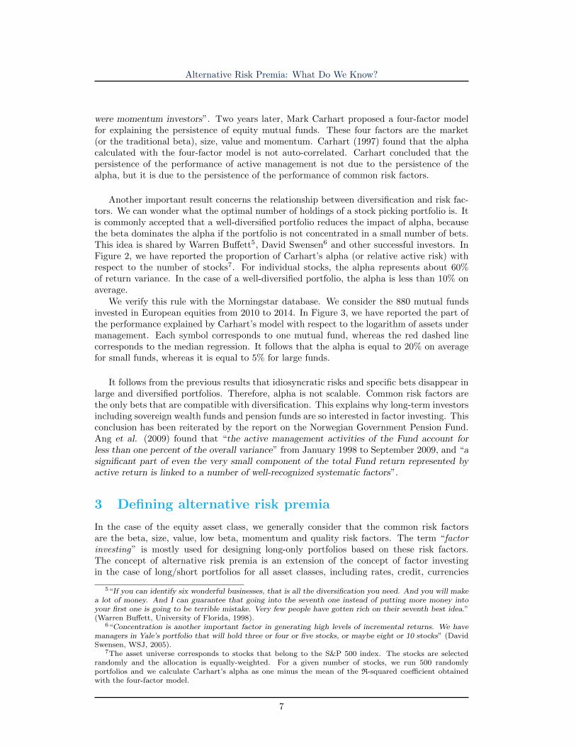
Another important result concerns the relationship between diversification and risk fac-tors. We can wonder what the optimal number of holdings of a stock picking portfolio is. Itis commonly accepted that a well-diversified portfolio reduces the impact of alpha, becausethe beta dominates the alpha if the portfolio is not concentrated in a small number of bets.This idea is shared by Warren Buffett5, David Swensen6 and other successful investors. InFigure 2, we have reported the proportion of Carhart’s alpha (or relative active risk) withrespect to the number of stocks7. For individual stocks, the alpha represents about 60%of return variance. In the case of a well-diversified portfolio, the alpha is less than 10% onaverage.

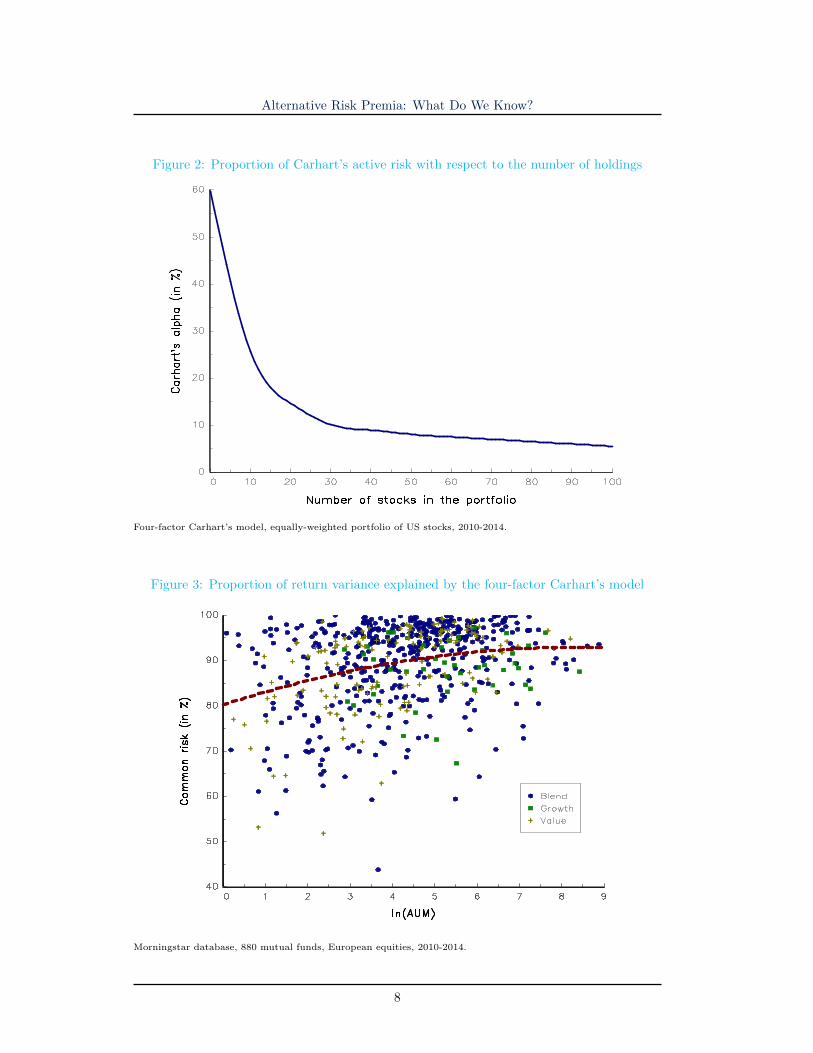
We verify this rule with the Morningstar database. We consider the 880 mutual fundsinvested in European equities from 2010 to 2014. In Figure 3, we have reported the part ofthe performance explained by Carhart’s model with respect to the logarithm of assets undermanagement. Each symbol corresponds to one mutual fund, whereas the red dashed linecorresponds to the median regression. It follows that the alpha is equal to 20% on averagefor small funds, whereas it is equal to 5% for large funds.

It follows from the previous results that idiosyncratic risks and specific bets disappear inlarge and diversified portfolios. Therefore, alpha is not scalable. Common risk factors arethe only bets that are compatible with diversification. This explains why long-term investorsincluding sovereign wealth funds and pension funds are so interested in factor investing. Thisconclusion has been reiterated by the report on the Norwegian Government Pension Fund.Ang et al. (2009) found that “the active management activities of the Fund account forless than one percent of the overall variance” from January 1998 to September 2009, and “asignificant part of even the very small component of the total Fund return represented byactive return is linked to a number of well-recognized systematic factors”.

3 Defining alternative risk premia

In the case of the equity asset class, we generally consider that the common risk factorsare the beta, size, value, low beta, momentum and quality risk factors. The term “factorinvesting” is mostly used for designing long-only portfolios based on these risk factors.The concept of alternative risk premia is an extension of the concept of factor investingin the case of long/short portfolios for all asset classes, including rates, credit, currencies

5“If you can identify six wonderful businesses, that is all the diversification you need. And you will makea lot of money. And I can guarantee that going into the seventh one instead of putting more money intoyour first one is going to be terrible mistake. Very few people have gotten rich on their seventh best idea.”(Warren Buffett, University of Florida, 1998).

6“Concentration is another important factor in generating high levels of incremental returns. We havemanagers in Yale’s portfolio that will hold three or four or five stocks, or maybe eight or 10 stocks” (DavidSwensen, WSJ, 2005).

7The asset universe corresponds to stocks that belong to the S&P 500 index. The stocks are selectedrandomly and the allocation is equally-weighted. For a given number of stocks, we run 500 randomlyportfolios and we calculate Carhart’s alpha as one minus the mean of the R-squared coefficient obtainedwith the four-factor model.

7


Figure 2: Proportion of Carhart’s active risk with respect to the number of holdings

Four-factor Carhart’s model, equally-weighted portfolio of US stocks, 2010-2014.

Figure 3: Proportion of return variance explained by the four-factor Carhart’s model

Morningstar database, 880 mutual funds, European equities, 2010-2014.

8


and commodities. It is interesting to notice that some asset classes, like currencies andcommodities, may exhibit alternative risk premia, but no traditional risk premia.

Alternative risk premia refer to non-traditional risk premia other than long-only ex-posures on equities and bonds. However, alternative risk premia also refer to alternativeinvestments and hedge fund strategies (Blin et al., 2017). Whereas factor investing affectsthe industry of equity active management, alternative risk premia is clearly a new analysisand investment framework for multi-asset allocation and portfolios of hedge funds.

3.1 Skewness risk premia and market anomalies

Strictly speaking, a risk premium rewards an exposure to a non-diversifiable or system-atic risk. For instance, the equity risk premium is defined as the reward that investorsexpect for being exposed to the equity risk. In fact, equity and bond risk premia are thetwo traditional risk premia. But there are other risk premia. A famous example is thepremium embedded in cat bonds, which are insurance-linked securities that transfer catas-trophe risks like hurricanes to investors. In this specific case, it is obvious that the risktaken by investors is non-diversifiable and non-hedgeable and must be rewarded. However,the existence of a risk premium is not always easy to justify for many strategies. Neverthe-less, the consumption-based model of Lucas (1978) helps to better characterize the conceptof risk premia. According to Cochrane (2001), the risk premium associated with an asset isequal to8:

Et [Rt+1 −Rf,t]︸︷︷︸Risk premium

∝ −ρ (u′ (Ct+1) , Rt+1)︸︷︷︸Correlation term

× σ (u′ (Ct+1))︸︷︷︸Smoothing term

× σ (Rt+1)︸︷︷︸Volatility term

(12)

where Rt+1 is the one-period return of the asset, Rf,t is the risk-free rate, Ct+1 is thefuture consumption and u (C) is the utility function. In bad times, investors decrease theirconsumption and the marginal utility is high. Therefore, investors agree to pay a high pricefor an asset that helps to smooth their consumption. To hedge bad times, investors can useassets with a low or negative risk premium. They will invest in assets that are positivelycorrelated with these bad times only if their risk premium is high. This is why investorsrequire a high risk premium in order to buy assets that are negatively correlated with themarginal utility and are highly volatile. Therefore, in the consumption-based model, therisk premium is compensation for accepting risk in bad times (Ang, 2014).

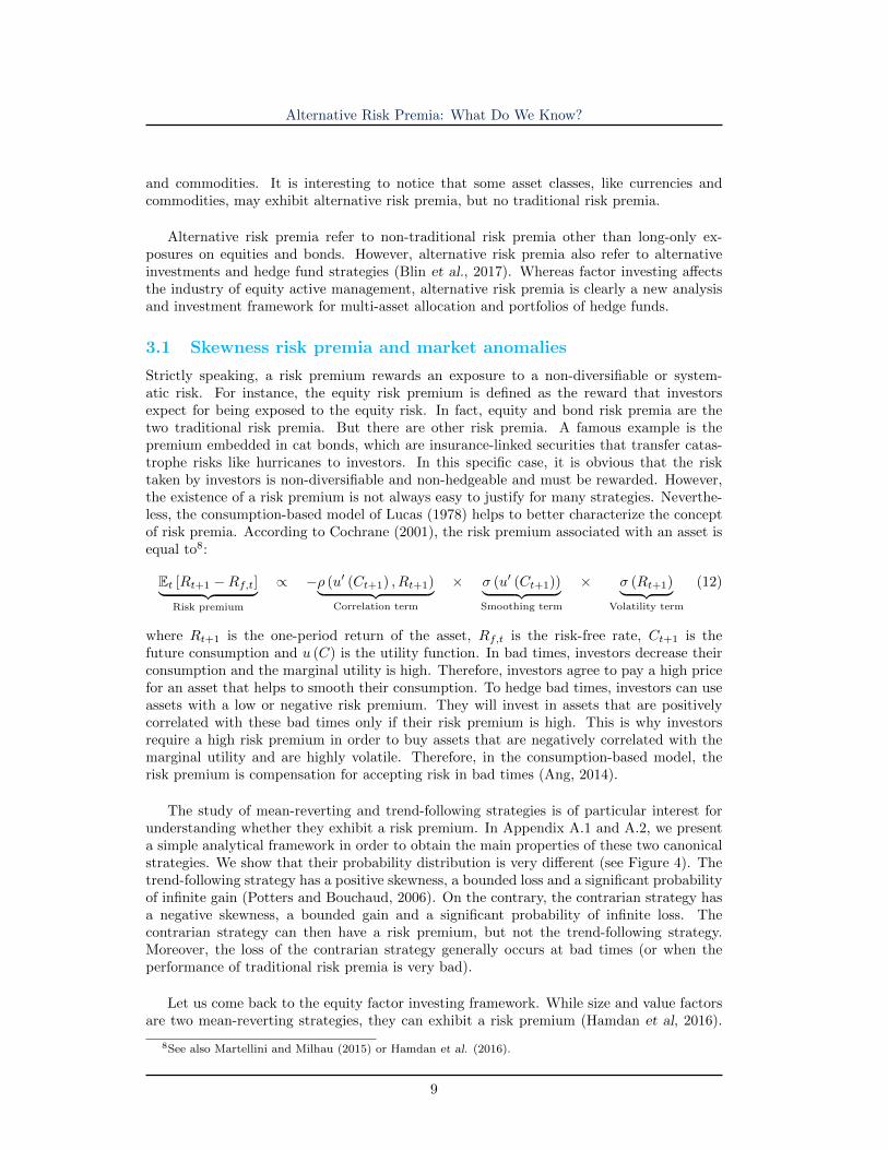
The study of mean-reverting and trend-following strategies is of particular interest forunderstanding whether they exhibit a risk premium. In Appendix A.1 and A.2, we presenta simple analytical framework in order to obtain the main properties of these two canonicalstrategies. We show that their probability distribution is very different (see Figure 4). Thetrend-following strategy has a positive skewness, a bounded loss and a significant probabilityof infinite gain (Potters and Bouchaud, 2006). On the contrary, the contrarian strategy hasa negative skewness, a bounded gain and a significant probability of infinite loss. Thecontrarian strategy can then have a risk premium, but not the trend-following strategy.Moreover, the loss of the contrarian strategy generally occurs at bad times (or when theperformance of traditional risk premia is very bad).

Let us come back to the equity factor investing framework. While size and value factorsare two mean-reverting strategies, they can exhibit a risk premium (Hamdan et al, 2016).

8See also Martellini and Milhau (2015) or Hamdan et al. (2016).

9


Figure 4: Probability density function of contrarian and trend-following strategies

This is not the case of the momentum risk factor. Concerning low beta and quality factors,there is no evidence that they reward a non-diversifiable risk during bad times. Here wehave precisely the opposite situation. During a stock market crisis, these two strategies aregenerally more resilient and outperform a buy-and-hold strategy in a cap-weighted index.Therefore, the good past performance of momentum, low beta and quality risk factors isnot due to a risk premium, but is explained by the theory of behavioral finance9. When astrategy has performed well in the past and it is not due to the existence of a risk premium,it is called a market anomaly (Hou et al., 2015).

In practice, investors and portfolio managers consider that alternative risk premia covertwo types of strategies:

1. The pure risk premia that are also called skewness risk premia.They correspond to the previous definition (Lemperiere et al., 2014). For example, thesize and value risk factors are two skewness risk premia.

2. The market anomalies.They correspond to trading strategies that have delivered good performance in thepast, but their performance cannot be explained by the existence of a systematic riskat bad times. Their performance can only be explained by behavioral theories. Forexample, the momentum, low beta and quality risk factors are three market anomalies.

9For instance, the momentum pattern may be explained by either an under-reaction to earnings an-nouncements and news, a delayed reaction, excessive optimism or pessimism, etc. (Barberis and Thaler,2003). The strong performance of low beta and low volatility assets may be explained by investors’ lever-age aversion (Frazzini and Pedersen, 2014). The quality strategy is another good example of strong andconsistent abnormal returns not related to risk (Asness et al., 2014).

10


Figure 5: Which option profile may exhibit a risk premium?

Figure 6: The case of a long straddle profile

11


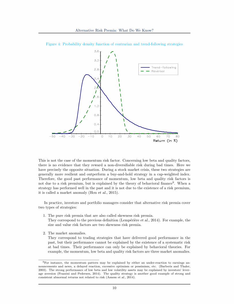
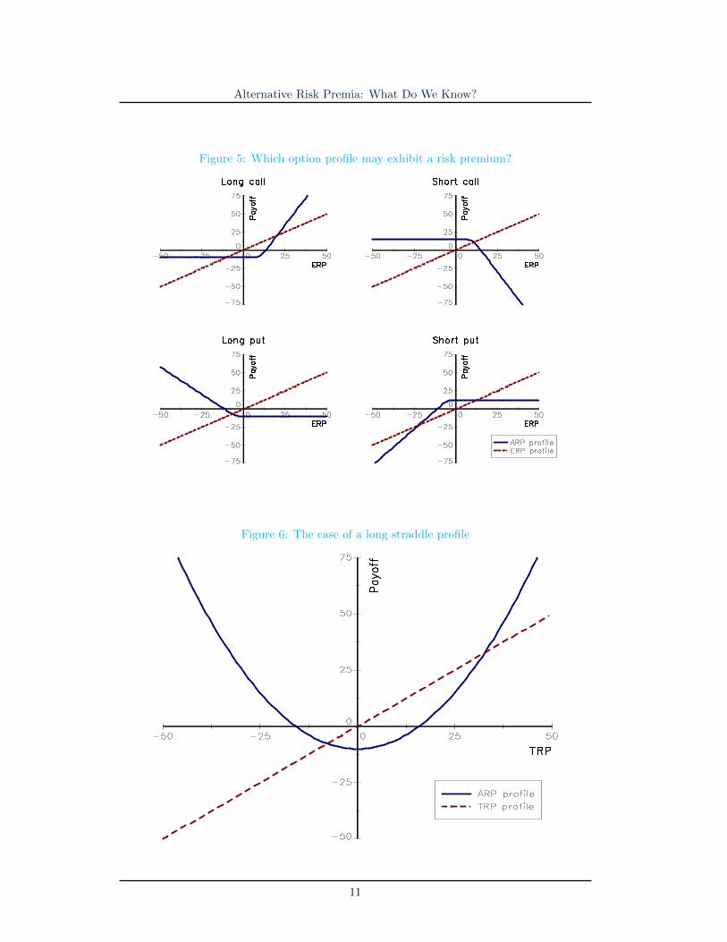
In order to better understand the difference between a skewness risk premium and a marketanomaly, we report generic payoffs of trading strategies with respect to the equity riskpremium (ERP) in Figure 5. In this case, bad times correspond to the drawdown of thestock market. If the payoff function of the trading strategy is a long call, it cannot be arisk premium, because the investor is not exposed to a skewness risk. Indeed, the loss ofthe trading strategy is limited and small. If the payoff function of the trading strategy isa long put, again it cannot be a risk premium, because the investor is rewarded in a bearmarket and this strategy hedges bad times. Therefore, this is an insurance premium andnot a risk premium. The case of the short call profile is interesting, because it exhibits adrawdown when the market is up. This means that the drawdown occurs in good times10

and not in bad times. If this trading strategy has a positive expected return, it can only be amarket anomaly, not a skewness risk premium. However, if the payoff function of the tradingstrategy is a short put, the investor takes a risk at bad times, when the performance of theequity market is negative. In this case, this type of strategy is a skewness risk premium11. Itis interesting to relate this analysis to the trend-following strategy on multi-asset classes12.Fung and Hsieh (2001) showed that this strategy has a long straddle option profile13 (Figure6). Based on our analysis, it is obvious that this strategy is a market anomaly, because itsdrawdown is not correlated to bad times.

3.2 Identification of alternative risk premia

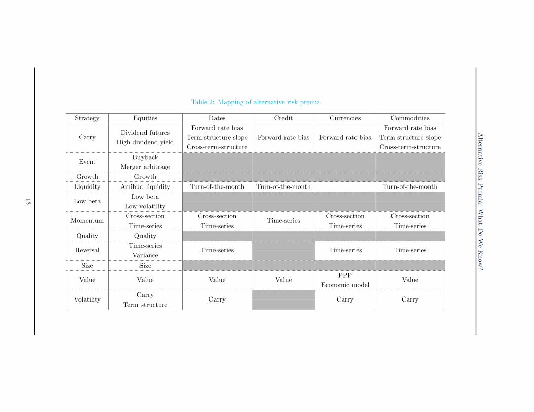
Identifying alternative risk premia is not an easy task, because there is no consensus. Forinstance, Harvey et al. (2016) found more than 300 academic publications that have exhib-ited new risk factors and tried to explain the cross-section of expected returns. They finallyconcluded that “most claimed research findings in financial economics are likely false”.Therefore, identifying alternative risk premia cannot be reduced to backtesting a strategyand performing a statistical analysis of past performance (Cochrane, 2011). In fact, theexistence of an alternative risk premium must be backed by the existence of investmentproducts, whose goal is indeed to harvest and replicate this risk premium. Otherwise, thismeans that the asset management industry does not believe in this risk premium. Thisunderlying idea is the starting point of the empirical study of Hamdan et al. (2016), whohave compiled a database of 1 120 existing indices, which are sponsored and calculated byasset managers, banks and index providers. They have classified these products accordingto the mapping shown in Table 2.

The different categories of risk premia are the following: carry, event, growth, liquidity,low beta, momentum, quality, reversal, size, value, volatility. This list is certainly non-exhaustive according to academic research. However, the asset management industry haseither not developed, or developed to a lesser extent, products based on the other categories,meaning that they are marginal from an investment point of view. Moreover, we notice thatsome categories of risk premia are not present in all asset classes. For instance, the event,growth, low beta, quality and size categories only concern the equity market. We also noticethat some risk premia can be implemented in several ways and correspond to differentstrategies. For instance, the equity carry risk premium corresponds to the high dividend

10When the stock market posts a very good performance.11This strategy has a negative skewness. However, a strategy that exhibits a short call option payoff may

also have a negative skewness. So, the value of the skewness can not be the only criterion. Indeed, theimportant point is when the skewness events occur. In some sense, the concept of skewness risk premia canbe related to the concept of the conditional co-skewness (Ilmanen, 2012).

12In the hedge fund industry, this strategy is known as the CTA strategy.13This strategy performs well when the market presents a significant (positive or negative) trend and posts

negative returns in rangy or reversal markets.

12

Altern

ativeR

iskP

remia:

Wh

atD

oW

eK

now

?

Table 2: Mapping of alternative risk premia

Strategy Equities Rates Credit Currencies Commodities

CarryDividend futures

High dividend yield

Forward rate bias Forward rate bias

Term structure slope Forward rate bias Forward rate bias Term structure slope

Cross-term-structure Cross-term-structure

EventBuyback

Merger arbitrage

Growth Growth

Liquidity Amihud liquidity Turn-of-the-month Turn-of-the-month Turn-of-the-month

Low betaLow beta

Low volatility

MomentumCross-section Cross-section

Time-seriesCross-section Cross-section

Time-series Time-series Time-series Time-series

Quality Quality

ReversalTime-series

Time-series Time-series Time-seriesVariance

Size Size

Value Value Value ValuePPP

ValueEconomic model

VolatilityCarry

Carry Carry CarryTerm structure

13


yield strategy and the dividend futures strategy. The first strategy consists in buildinga portfolio that is long on stocks with high dividend yields and short on stocks with lowdividend yields. The aim of the second strategy consists in capturing the difference betweenimplied and realized dividends.

Let us briefly define the different categories14. The underlying idea of a carry strategyis to capture a spread or a return by betting that the underlying risk will not occur or thatmarket conditions will stay the same (Koijen et al., 2017; Baltas, 2017). One famous exampleof such a strategy is the currency carry trade. It consists in being long on currencies withhigh interest rates and short on currencies with low interest rates. If exchange rates do notchange, this portfolio generates a positive return. In the case of bonds and commodities,we generally distinguish between several forms of carry strategies, depending on whetherthe carry is calculated using one maturity of the term structure (forward rate bias), twomaturities of the same term structure (term structure slope) or one maturity of two differentterm structures (cross-yield curve).

The event category covers several idiosyncratic risk strategies, like merger arbitrage,convertible arbitrage and buyback strategy. The growth strategy consists in selecting stocksof companies that are growing substantially faster than others. Contrary to popular belief,this is not the same as the anti-value strategy.

In the liquidity category, we find strategies whose goal is to capture the illiquidity pre-mium of some assets (Pastor and Stambaugh, 2003). In the equity asset class, the mostpopular illiquidity measure is the Amihud ratio (Amihud, 2002). In the other asset classes,liquidity strategies consist in market timing strategies and generally exploit the turn-of-the-month effect. Indeed, some (passive) investors have to roll futures contracts at somepre-defined periods, resulting in liquidity pressures around these rolling periods. The lowbeta anomaly consists in building a portfolio with exposure to low volatility stocks.

Two strategies define the momentum risk premium: cross-section momentum (Jegadeeshand Titman, 1993) and time-series momentum (Moskowitz et al., 2012). The two strategiesassume that the past trend is a predictor of the future trend. The cross-section momentumstrategy consists in building a portfolio that is long on assets that have outperformed andshort on assets that have underperformed. In the case of the time-series momentum strategy,the portfolio is long on assets with a positive past trend and short on assets with a negativepast trend15.

The quality factor is a market anomaly that cannot be explained by a risk premium. Ithas been exhibited by Piotroski (2000) and the strategy corresponds to a portfolio long onquality stocks and short on junk stocks without any reference to market prices (Asness et al.,2014). Typical quality measures include equity-to-debt, return-on-equity or income-to-salesfinancial ratios.

The reversal strategy is also known as the contrarian or the mean-reverting strategy. Insome sense, it is the opposite of the trend-following strategy. For an asset class, the twostrategies can coexist because they do not involve the same time frequency. For instance, inthe case of equities, it is widely recognized that the market is contrarian in the short term

14See Hamdan et al. (2016) for a detailed explanation of each category of risk premia and the relatedstrategies.

15Whereas cross-section momentum is related to relative returns, time-series momentum considers absolutereturns.

14


(less than one month), trend-following in the medium term (between one month and twoyears) and mean-reverting in the long run (greater than two years). When we speak aboutthe reversal premium, we generally consider the short-term contrarian strategy, whereas thelong-term mean reverting strategy is classified with the value risk premium. Like manyalternative risk premia, there are several ways to implement such a strategy. For example,it can use short-term trends (time-series reversal) or variance differences of returns betweentwo time horizons (variance reversal).

The underlying idea of the size factor is that small stocks have a natural excess returnwith respect to large stocks. This excess return may be explained by a liquidity premium orbecause this market is less efficient than a market of large caps. In the asset managementindustry, this factor is only implemented in the equity asset class.

The value equity factor was popularized by Fama and French (1993, 1998). This strategygoes long on under-valuated stocks and short on over-valuated stocks. Whereas Fama andFrench use the price-to-book value ratio as the value measure, asset managers generally com-bine different financial ratios (earnings yield, dividend yield, etc.). Choosing the approachto implement the value factor is crucial, because it impacts the nature of the captured riskpremium. Some products focus on the short-term value premium, whereas the majorityof products try to capture the long-term value premium or the fundamental component ofthe value premium. In the other asset classes, the value strategy corresponds more to along-term contrarian strategy. There are generally two main approaches for defining thelong-run fundamental price. The first approach uses economic models whereas the secondapproach consists in estimating the long-run equilibrium price using statistical methods.

The last risk premium concerns the volatility asset class. The volatility carry risk pre-mium corresponds to a portfolio that captures the spread between implied volatility andrealized volatility. It is also known as the short volatility strategy. Another strategy con-cerns the term structure of VIX futures contracts, and aims to capture the roll-down effectof the slope of the term structure.

In Table 2, we notice that some risk premia are not present in all asset classes, becausethey are not implemented in the industry of financial indices16. This mapping was valid atthe end of December 2015. It does not mean that it will continue to be valid in the comingyears. For example, there have been some recent attempts by asset managers to apply thequality factor to the fixed-income universe. Another identification issue is the robustness ofa given category. If a category contains very few products, we can consider that the riskpremium is anecdotal. For example, Hamdan et al. (2006) only found three momentumrisk premium indices on the US credit asset class. In this case, we may wonder if this riskpremium really exists.

For a risk premium to be robust, there must be a sufficient number of products but theyalso must be sufficiently homogenous in order to represent the same common risk factor. Letus consider the case of the traditional equity risk premium in the US market. The investorhas the choice between different indices to harvest this risk premium. Selecting the index isa minor problem, because the correlation between the different indices is very high17. This

16Of course, they can be implemented in other forms by the asset management industry. For example,the event factor on fixed-income instruments is implemented by some hedge funds. The fact that there isno index means that it is more a ‘discretionary’ strategy than a risk premium. In this case, the skill of thefund manager is essential to deliver good performance.

17For example, the cross-correlation between the daily returns of the S&P 500, FTSE USA, MSCI USA,Russell 1000 and Russell 3000 indices was greater than 99.5% between 2000 and 2015.

15


is not the case with alternative risk premia. Suppose that we have a category with fiveindices and that the cross-correlation between them is lower than 50%. In this case, we canbelieve that this category is more representative of a strategy than a risk premium. Indeed,the performance will be explained more by the portfolio construction than the intrinsicreturn of the common risk factor. In order to obtain a homogeneous category, Hamdanet al. (2016) proposed a selection procedure in order to estimate the generic performanceof the risk premium. They found that some categories are so heterogeneous that it is notpossible to obtain a subset of indices that present the same patterns. This is the case withthe following strategies: the carry risk premium based on dividend futures, the liquiditypremium in equities, rates and currencies, the value risk premium in rates and commodities,the reversal risk premium based on the variance approach and risk premia in the creditmarket.

3.3 Carry and momentum everywhere

According to Hamdan et al. (2016), the most important18 risk premia in equities are thevalue risk factor, followed by the carry based on the high dividend yield approach, the lowvolatility, the short volatility and the momentum risk factor. In the case of currencies andcommodities, the two important risk premia are the carry and momentum strategies. Forthe fixed-income asset class, these same risk premia are important, in addition to the shortvolatility strategy.

We notice that carry and momentum are the most relevant alternative risk premia.We find them in the four asset classes, even if they are differently implemented. Thisis particularly true for the carry risk premium. It corresponds to strategies on the termstructure for rates and commodities, and income strategies for equities and currencies. Italso encompasses the famous short volatility strategy. For the momentum risk premium,both cross-section and time-series strategies are appropriate.

The title of this section refers to the article of Asness et al. (2013) entitled ‘Value andMomentum Everywhere’, that found “significant return premia to value and momentum inevery asset class”. The difference comes from the fact that the approach of Asness et al.(2013) is based on backtesting whereas the approach of Hamdan et al. (2016) is based on theexistence of current investment indices. It is interesting to notice that the asset managementindustry believes more in carry than in value, except for the equity asset class. This resultmay change in the future. For example, some recent research also exhibits a value pattern inthe universe of corporate bonds (Bektic et al., 2017; Houweling and van Zundert, 2017; Israelet al., 2016). However, it is unlikely that the value risk premium enjoys the same status ascarry and momentum in the case of commodities and currencies. The issue comes from themean-reverting frequency of the value strategy. When the frequency is very low (e.g. fiveyears), it is extremely difficult for the asset management industry to propose investmentvehicles with such a long time horizon, but investors can always implement such a strategyat their own level. In the case of equities, two value strategies exist with two different mean-reverting frequencies19. The success of the value strategy in the equity space comes fromthe mixing of these two time horizons, which are shorter than the value frequency observedin the other asset classes.

18The importance is measured in terms of the number of homogenous indices within the category.19A short-term strategy with a one-month frequency and a strategy, whose frequency is more than two

years. For instance, Bourguignon and de Jong (2006) broke down the performance of the value strategyinto a transitory time component and a structural time component. They showed that a large part of theperformance is explained by the short-term component.

16


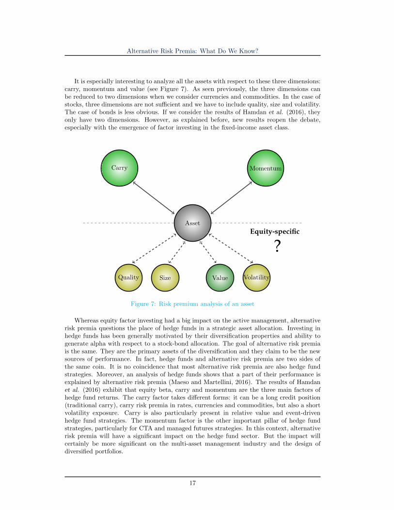
It is especially interesting to analyze all the assets with respect to these three dimensions:carry, momentum and value (see Figure 7). As seen previously, the three dimensions canbe reduced to two dimensions when we consider currencies and commodities. In the case ofstocks, three dimensions are not sufficient and we have to include quality, size and volatility.The case of bonds is less obvious. If we consider the results of Hamdan et al. (2016), theyonly have two dimensions. However, as explained before, new results reopen the debate,especially with the emergence of factor investing in the fixed-income asset class.

Equity-specific

?

Carry Momentum

Asset

Quality Size Value Volatility

Figure 7: Risk premium analysis of an asset

Whereas equity factor investing had a big impact on the active management, alternativerisk premia questions the place of hedge funds in a strategic asset allocation. Investing inhedge funds has been generally motivated by their diversification properties and ability togenerate alpha with respect to a stock-bond allocation. The goal of alternative risk premiais the same. They are the primary assets of the diversification and they claim to be the newsources of performance. In fact, hedge funds and alternative risk premia are two sides ofthe same coin. It is no coincidence that most alternative risk premia are also hedge fundstrategies. Moreover, an analysis of hedge funds shows that a part of their performance isexplained by alternative risk premia (Maeso and Martellini, 2016). The results of Hamdanet al. (2016) exhibit that equity beta, carry and momentum are the three main factors ofhedge fund returns. The carry factor takes different forms: it can be a long credit position(traditional carry), carry risk premia in rates, currencies and commodities, but also a shortvolatility exposure. Carry is also particularly present in relative value and event-drivenhedge fund strategies. The momentum factor is the other important pillar of hedge fundstrategies, particularly for CTA and managed futures strategies. In this context, alternativerisk premia will have a significant impact on the hedge fund sector. But the impact willcertainly be more significant on the multi-asset management industry and the design ofdiversified portfolios.

17


4 Portfolio allocation with alternative risk premia

Using a universe of alternative risk premia makes the asset allocation policy more difficultthan using traditional risk premia. First, alternative risk premia are generally long-shortstrategies. It may be difficult to understand the behavior of some ARP with respect to atraditional long exposure on equities or bonds. Second, the skewness risk cannot be ignoredand must be managed.

4.1 Volatility diversification

Let X1 and X2 be two random variables. The volatility of the sum is less than the sum ofindividual volatilities:

σ (X1 +X2) ≤ σ (X1) + σ (X2) (13)

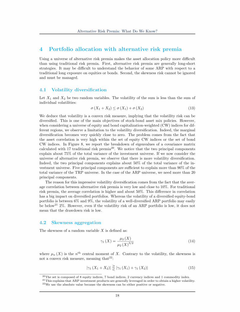
We deduce that volatility is a convex risk measure, implying that the volatility risk can bediversified. This is one of the main objectives of stock-bond asset mix policies. However,when considering a universe of equity and bond capitalization-weighted (CW) indices for dif-ferent regions, we observe a limitation to the volatility diversification. Indeed, the marginaldiversification becomes very quickly close to zero. The problem comes from the fact thatthe asset correlation is very high within the set of equity CW indices or the set of bondCW indices. In Figure 8, we report the breakdown of eigenvalues of a covariance matrixcalculated with 17 traditional risk premia20. We notice that the two principal componentsexplain about 75% of the total variance of the investment universe. If we now consider theuniverse of alternative risk premia, we observe that there is more volatility diversification.Indeed, the two principal components explains about 50% of the total variance of the in-vestment universe. Five principal components are sufficient to explain more than 90% of thetotal variance of the TRP universe. In the case of the ARP universe, we need more than 20principal components.

The reason for this impressive volatility diversification comes from the fact that the aver-age correlation between alternative risk premia is very low and close to 10%. For traditionalrisk premia, the average correlation is higher and about 50%. This difference in correlationhas a big impact on diversified portfolios. Whereas the volatility of a diversified equity-bondportfolio is between 6% and 9%, the volatility of a well-diversified ARP portfolio may easilybe below21 2%. However, even if the volatility risk of an ARP portfolio is low, it does notmean that the drawdown risk is low.

4.2 Skewness aggregation

The skewness of a random variable X is defined as:

γ1 (X) =µ3 (X)

µ2 (X)3/2

(14)

where µn (X) is the nth central moment of X. Contrary to the volatility, the skewness isnot a convex risk measure, meaning that22:

|γ1 (X1 +X2)| T |γ1 (X1) + γ1 (X2)| (15)

20The set is composed of 8 equity indices, 7 bond indices, 2 currency indices and 1 commodity index.21This explains that ARP investment products are generally leveraged in order to obtain a higher volatility.22We use the absolute value because the skewness can be either positive or negative.

18


Figure 8: Principal component analysis of TRP and ARP investment universes

Source: Hamdan et al. (2016).

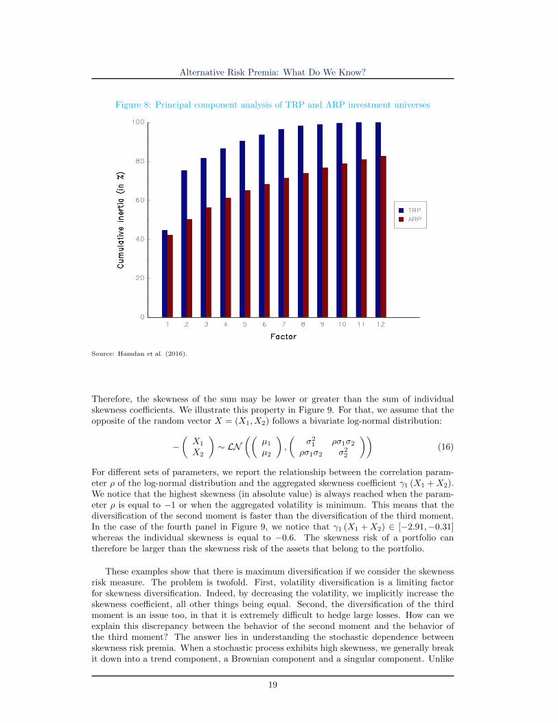
Therefore, the skewness of the sum may be lower or greater than the sum of individualskewness coefficients. We illustrate this property in Figure 9. For that, we assume that theopposite of the random vector X = (X1, X2) follows a bivariate log-normal distribution:

−(X1

X2

)∼ LN

((µ1

µ2

),

(σ2

1 ρσ1σ2

ρσ1σ2 σ22

))(16)

For different sets of parameters, we report the relationship between the correlation param-eter ρ of the log-normal distribution and the aggregated skewness coefficient γ1 (X1 +X2).We notice that the highest skewness (in absolute value) is always reached when the param-eter ρ is equal to −1 or when the aggregated volatility is minimum. This means that thediversification of the second moment is faster than the diversification of the third moment.In the case of the fourth panel in Figure 9, we notice that γ1 (X1 +X2) ∈ [−2.91,−0.31]whereas the individual skewness is equal to −0.6. The skewness risk of a portfolio cantherefore be larger than the skewness risk of the assets that belong to the portfolio.

These examples show that there is maximum diversification if we consider the skewnessrisk measure. The problem is twofold. First, volatility diversification is a limiting factorfor skewness diversification. Indeed, by decreasing the volatility, we implicitly increase theskewness coefficient, all other things being equal. Second, the diversification of the thirdmoment is an issue too, in that it is extremely difficult to hedge large losses. How can weexplain this discrepancy between the behavior of the second moment and the behavior ofthe third moment? The answer lies in understanding the stochastic dependence betweenskewness risk premia. When a stochastic process exhibits high skewness, we generally breakit down into a trend component, a Brownian component and a singular component. Unlike

19


Figure 9: Illustration of skewness aggregation with the bivariate log-normal distribution

regular and irregular variations that are easy to diversify, it is difficult to hedge discontinuousvariations. In their simplest form, these singular variations are jumps. The worst-casescenario concerning skewness aggregation is thus to build a well-diversified portfolio bydramatically reducing the volatility of the portfolio. Indeed, it is extremely difficult todiversify the negative jump of an asset. For that, we need to find a second asset that jumpsat the same time and has a positive jump. Moreover, bad times of skewness risk premia tendto occur at the same time. By accumulating alternative risk premia, we then increase thevolatility diversification and reduce the absolute value of the drawdown, but the drawdownof the portfolio compared to its realized volatility appears to be very high. This explainsthat the Sharpe ratio is not the right measure for evaluating the risk/return ratio of an ARPportfolio.

4.3 Portfolio management

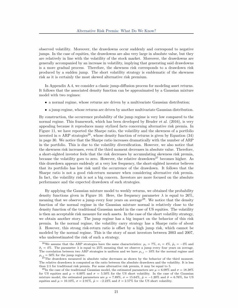
In order to establish clear rules about asset allocation, we have to understand the significanceof the skewness risk23. In the top panel in Figure 10, we report the cumulative performanceof US equities24 and the US volatility carry premium25. If we consider weekly returns, itappears that the skewness of the US volatility carry premium is 13 times the skewness ofUS equities. This high skewness risk is explained by the magnitude of historical drawdownswith respect to the historical volatility. Indeed, we notice that the short volatility strategyexperienced very low volatility most of times, implying that this risk premium seems tohave a very low risk during long historical periods. However, in a period of stress, the shortvolatility strategy may suffer greatly, and its drawdowns appear very large compared to the

23See Jurczenko and Maillet (2006) for a review of the literature on portfolio management with skewness.24It is approximated by the S&P 500 index25We use the generic performance of the US short volatility strategy obtained by Hamdan et al. (2016).

20


observed volatility. Moreover, the drawdowns occur suddenly and correspond to negativejumps. In the case of equities, the drawdowns are also very large in absolute value, but theyare relatively in line with the volatility of the stock market. Moreover, the drawdowns aregenerally accompanied by an increase in volatility, implying that generating said drawdownsis a more gradual process. Therefore, the skewness risk corresponds to a drawdown riskproduced by a sudden jump. The short volatility strategy is emblematic of the skewnessrisk as it is certainly the most skewed alternative risk premium.

In Appendix A.4, we consider a classic jump-diffusion process for modeling asset returns.It follows that the associated density function can be approximated by a Gaussian mixturemodel with two regimes:

• a normal regime, whose returns are driven by a multivariate Gaussian distribution;

• a jump regime, whose returns are driven by another multivariate Gaussian distribution.

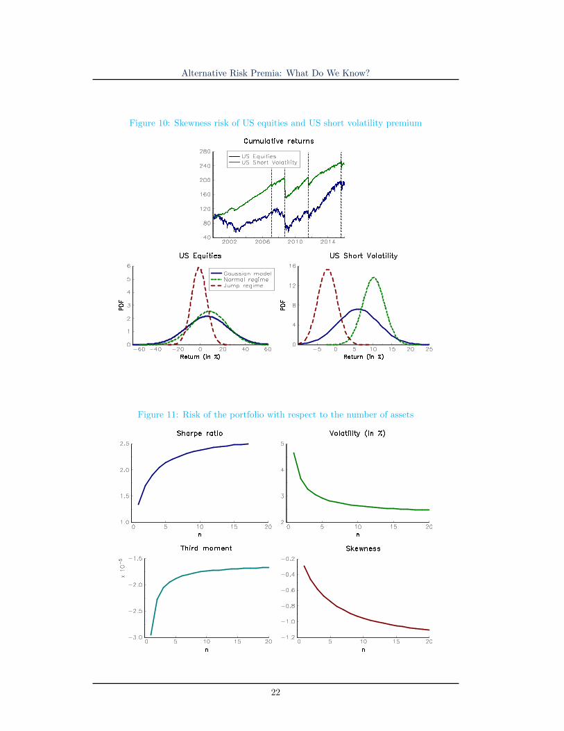
By construction, the occurrence probability of the jump regime is very low compared to thenormal regime. This framework, which has been developed by Bruder et al. (2016), is veryappealing because it reproduces many stylized facts concerning alternative risk premia. InFigure 11, we have reported the Sharpe ratio, the volatility and the skewness of a portfolioinvested in n ARP strategies26, whose density function of returns is given by Equation (34)in page 30. We notice that the Sharpe ratio increases dramatically with the number of ARPin the portfolio. This is due to the volatility diversification. However, we also notice thatthe skewness risk increases, even if the third moment decreases in absolute value. Therefore,a short-sighted investor feels that the risk decreases by accumulating skewness risk premia,because the volatility goes to zero. However, the relative drawdown27 becomes higher. Asthis drawdown appears suddenly at a very low frequency, the short-sighted investor believesthat its portfolio has low risk until the occurrence of the drawdown. It follows that theSharpe ratio is not a good risk-return measure when considering alternative risk premia.In fact, the volatility risk is not a big concern. Investors are more focused on the absoluteperformance and the expected drawdown of such strategies.

By applying the Gaussian mixture model to weekly returns, we obtained the probabilitydensity functions given in Figure 10. Here, the frequency parameter λ is equal to 26%,meaning that we observe a jump every four years on average28. We notice that the densityfunction of the normal regime in the Gaussian mixture normal is relatively close to thedensity function of the traditional Gaussian model in the case of US equities. The volatilityis then an acceptable risk measure for such assets. In the case of the short volatility strategy,we obtain another story. The jump regime has a big impact on the behavior of this riskpremia. In the normal regime, the volatility carry strategy has a Sharpe ratio of about3. However, this strong risk-return ratio is offset by a high jump risk, which cannot bemodeled by the normal regime. This is the story of most investors between 2003 and 2007,who underestimated the risk of such a strategy.

26We assume that the ARP strategies have the same characteristics: µi = 7%, σi = 4%, µi = −3% andσi = 4%. The parameter λ is equal to 25% meaning that we observe a jump every four years on average.The correlation between two ARP strategies is uniform and we have ρi,j = 10% for the normal regime andρi,j = 50% for the jump regime.

27The drawdown measured in absolute value decreases as shown by the behavior of the third moment.The relative drawdown is computed as the ratio between the absolute drawdown and the volatility. It is lessthan 2.5 for traditional risk premia. For some alternative risk premia, it may be equal to 5.

28In the case of the traditional Gaussian model, the estimated parameters are µ = 6.09% and σ = 18.38%for US equities and µ = 6.00% and σ = 5.50% for the US short volatility. In the case of the Gaussianmixture model, the estimated parameters are µ = 7.89%, σ = 15.64%, µ = −1.20% and σ = 6.76%, for USequities and µ = 10.10%, σ = 2.91%, µ = −2.23% and σ = 2.57% for the US short volatility.

21


Figure 10: Skewness risk of US equities and US short volatility premium

Figure 11: Risk of the portfolio with respect to the number of assets

22


We have seen previously that risk budgeting is the right approach for building a diversifiedportfolio, and alternative risk premia are the common risk factors for diversifying a strategicasset allocation. Therefore, professionals have naturally combined the two approaches inorder to provide well-diversified multi-asset portfolios. Generally, the construction of theportfolio is a two-stage process. First, the manager selects the best alternative risk premia.Second, the portfolio is rebalanced at a fixed frequency by defining volatility risk budgets.However, we have seen that the volatility is certainly not relevant to assess the risk ofskewness risk premia, because we cannot manage their bad times with a traditional riskparity method29. Moreover, the occurrence of a drawdown of a given skewness risk premiumis followed by an increase of the realized volatility, implying that the risk parity portfolioreduces dramatically the allocation on this strategy. However, it is generally too late. Ifwe consider again the short volatility strategy, we notice that the strategy rebounds sharplyafter a drawdown. Therefore, the optimal investment decision is not to reduce, but tomaintain or increase the exposure.

Bruder et al. (2016) propose to replace the volatility risk measure of the risk budgetingmethod by the expected shortfall30 based on the Gaussian mixture model. Their approachhas the advantage of taking into account the skewness risk and eliminating the jumps in theallocation. This allocation is then more stable, because the risk measure integrates ex-antethe jump risk, meaning that the dynamic of the allocation is mainly driven by the truevolatility and not by jumps. This point is very important, because we understand that thenature of the skewness risk is different than the nature of the volatility risk in terms ofallocation dynamics. The skewness risk is a decision of strategic asset allocation, implyingthat the investor must allocate a skewness risk budget for each risk premium in the long-runand stick to this allocation even if a drawdown occurs. The volatility risk is a decision oftactical asset allocation, implying that the investor may dynamically change the allocationby considering the true volatility of risk premia. Therefore, the challenge is to separatevolatility and skewness effects. For instance, the empirical volatility is a biased estimatorof the true volatility, because it incorporates jumps. This is why we have to adopt filteringapproaches for estimating the volatility of alternative risk premia.

The approach of Bruder et al. (2016) can be simplified as follows. Suppose that wewould like to allocate the risk budgets b1, . . . , bn to a universe of n risk premia. The ideais to transform these risk budgets that incorporate the skewness risk into new risk budgetsb′1, . . . , b

′n that are only based on the volatility risk. We can then manage the portfolio by

using a traditional risk budgeting approach and a filtered covariance matrix, which do nottake into account skewness events. This simplified approach shows that skewness risk premiaand market anomalies do not have the same status. For instance, if we wanted to allocatethe same risk budget between a skewness risk premium and a market anomaly, this impliesthat the volatility budget will be higher for the market anomaly.

29By traditional risk party, we mean an equal risk contribution portfolio based on the volatility riskmeasure.

30See also Jurczenko and Teıletche (2015) and Roncalli (2015) for risk budgeting methods based on theexpected shortfall.

23


5 Conclusion

Alternative risk premia cover two types of strategy: skewness risk premia and market anoma-lies. Skewness risk premia reward systematic risks taken by investors in bad times. Anexample is the short volatility strategy, and more generally carry strategies. Market anoma-lies correspond to trading strategies that have delivered good performance in the past, buttheir performance can be explained by behavioral theories, but not by a skewness risk. Forinstance, momentum is a market anomaly.

Diversification covers two main risks: volatility risk and skewness risk. It is very impor-tant to understand that volatility diversification is very different to skewness diversification.In particular, managing the skewness risk is a strategic asset allocation decision, whereasmanaging the volatility risk is a tactical asset allocation decision. Moreover, we notice thatit is extremely difficult to hedge the skewness risk, because there is a floor to skewnessdiversification.

Alternative risk premia and diversification are highly related. Until recently, multi-assetallocation was reduced to stock-bond and country allocation. Alternative risk premia arenow an extension to the traditional risk premia universe. Investors have then a large choiceof building blocks or primary assets. Of course, this new approach challenges the placeof hedge funds in a strategic asset allocation. Moreover, it also participates in the debateabout alpha versus beta, but also in the debate about passive management versus activemanagement. Every day, the importance of alpha is decreasing alarmingly, implying that theportfolio performance is mainly explained by systematic risk factors and not by specific riskfactors. And the emergence of alternative risk premia renews risk/return and benchmarkinganalysis. However, it does not mean that active management does not play an importantrole in this context. Whereas it is more efficient to capture traditional betas using passivemanagement, it is not straightforward that it is the same thing for alternative betas. Let ustake the case of carry and momentum risk premia. Even if these two premia are theoreticallywell-defined, there are many ways for implementing them. We can harvest them using anindex that encapsulates a fully detailed systematic strategy or using a portfolio manager thatconsiders a more sophisticated quantitative model, which can be adapted to the investmentand liquidity environment31. Certainly, these two approaches will co-exist, meaning thatthe shift of active management from alpha towards alternative risk premia has just begun.

This chapter is dedicated to alternative risk premia based on traditional financial assets(equities, rates, credit, currencies and commodities). Another important question concernsthe place of risk premia on ‘alternative’ assets (real estate, private debt, private equity,infrastructure) in a strategic asset allocation. By construction, the asset allocation policybetween these risk premia cannot be driven by volatility diversification. Therefore, skew-ness32 diversification remains the main issue when managing a portfolio of real assets.

31Moreover, the allocation between alternative risk premia with respect to macro-economic factors remainsan open question for active management.

32in a very broad sense including cross-skewness and time-skewness management.

24


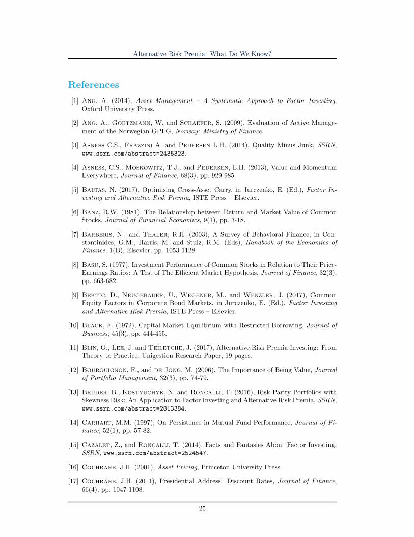
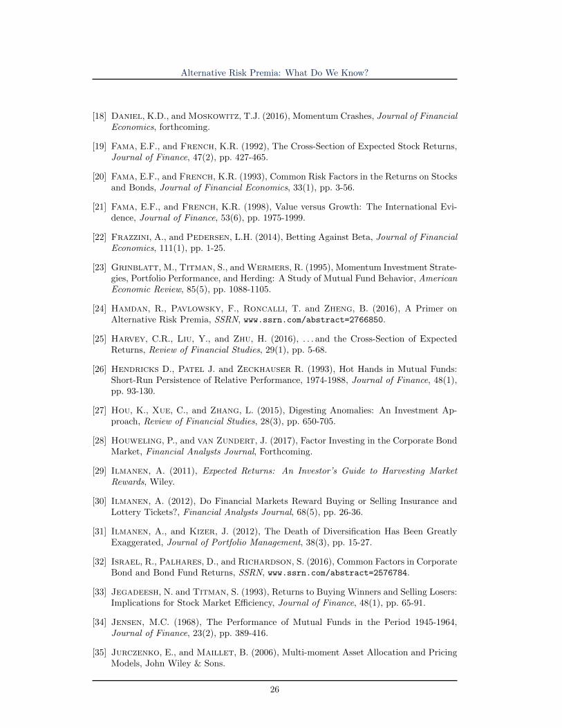
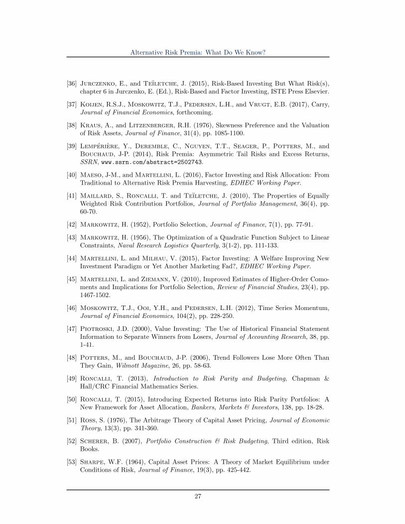
References

[1] Ang, A. (2014), Asset Management – A Systematic Approach to Factor Investing,Oxford University Press.

[2] Ang, A., Goetzmann, W. and Schaefer, S. (2009), Evaluation of Active Manage-ment of the Norwegian GPFG, Norway: Ministry of Finance.

[3] Asness C.S., Frazzini A. and Pedersen L.H. (2014), Quality Minus Junk, SSRN,www.ssrn.com/abstract=2435323.

[4] Asness, C.S., Moskowitz, T.J., and Pedersen, L.H. (2013), Value and MomentumEverywhere, Journal of Finance, 68(3), pp. 929-985.

[5] Baltas, N. (2017), Optimising Cross-Asset Carry, in Jurczenko, E. (Ed.), Factor In-vesting and Alternative Risk Premia, ISTE Press – Elsevier.

[6] Banz, R.W. (1981), The Relationship between Return and Market Value of CommonStocks, Journal of Financial Economics, 9(1), pp. 3-18.

[7] Barberis, N., and Thaler, R.H. (2003), A Survey of Behavioral Finance, in Con-stantinides, G.M., Harris, M. and Stulz, R.M. (Eds), Handbook of the Economics ofFinance, 1(B), Elsevier, pp. 1053-1128.

[8] Basu, S. (1977), Investment Performance of Common Stocks in Relation to Their Price-Earnings Ratios: A Test of The Efficient Market Hypothesis, Journal of Finance, 32(3),pp. 663-682.

[9] Bektic, D., Neugebauer, U., Wegener, M., and Wenzler, J. (2017), CommonEquity Factors in Corporate Bond Markets, in Jurczenko, E. (Ed.), Factor Investingand Alternative Risk Premia, ISTE Press – Elsevier.

[10] Black, F. (1972), Capital Market Equilibrium with Restricted Borrowing, Journal ofBusiness, 45(3), pp. 444-455.

[11] Blin, O., Lee, J. and Teıletche, J. (2017), Alternative Risk Premia Investing: FromTheory to Practice, Unigestion Research Paper, 19 pages.

[12] Bourguignon, F., and de Jong, M. (2006), The Importance of Being Value, Journalof Portfolio Management, 32(3), pp. 74-79.

[13] Bruder, B., Kostyuchyk, N. and Roncalli, T. (2016), Risk Parity Portfolios withSkewness Risk: An Application to Factor Investing and Alternative Risk Premia, SSRN,www.ssrn.com/abstract=2813384.

[14] Carhart, M.M. (1997), On Persistence in Mutual Fund Performance, Journal of Fi-nance, 52(1), pp. 57-82.

[15] Cazalet, Z., and Roncalli, T. (2014), Facts and Fantasies About Factor Investing,SSRN, www.ssrn.com/abstract=2524547.

[16] Cochrane, J.H. (2001), Asset Pricing, Princeton University Press.

[17] Cochrane, J.H. (2011), Presidential Address: Discount Rates, Journal of Finance,66(4), pp. 1047-1108.

25


[18] Daniel, K.D., and Moskowitz, T.J. (2016), Momentum Crashes, Journal of FinancialEconomics, forthcoming.

[19] Fama, E.F., and French, K.R. (1992), The Cross-Section of Expected Stock Returns,Journal of Finance, 47(2), pp. 427-465.

[20] Fama, E.F., and French, K.R. (1993), Common Risk Factors in the Returns on Stocksand Bonds, Journal of Financial Economics, 33(1), pp. 3-56.

[21] Fama, E.F., and French, K.R. (1998), Value versus Growth: The International Evi-dence, Journal of Finance, 53(6), pp. 1975-1999.

[22] Frazzini, A., and Pedersen, L.H. (2014), Betting Against Beta, Journal of FinancialEconomics, 111(1), pp. 1-25.

[23] Grinblatt, M., Titman, S., and Wermers, R. (1995), Momentum Investment Strate-gies, Portfolio Performance, and Herding: A Study of Mutual Fund Behavior, AmericanEconomic Review, 85(5), pp. 1088-1105.

[24] Hamdan, R., Pavlowsky, F., Roncalli, T. and Zheng, B. (2016), A Primer onAlternative Risk Premia, SSRN, www.ssrn.com/abstract=2766850.

[25] Harvey, C.R., Liu, Y., and Zhu, H. (2016), . . . and the Cross-Section of ExpectedReturns, Review of Financial Studies, 29(1), pp. 5-68.

[26] Hendricks D., Patel J. and Zeckhauser R. (1993), Hot Hands in Mutual Funds:Short-Run Persistence of Relative Performance, 1974-1988, Journal of Finance, 48(1),pp. 93-130.

[27] Hou, K., Xue, C., and Zhang, L. (2015), Digesting Anomalies: An Investment Ap-proach, Review of Financial Studies, 28(3), pp. 650-705.

[28] Houweling, P., and van Zundert, J. (2017), Factor Investing in the Corporate BondMarket, Financial Analysts Journal, Forthcoming.

[29] Ilmanen, A. (2011), Expected Returns: An Investor’s Guide to Harvesting MarketRewards, Wiley.

[30] Ilmanen, A. (2012), Do Financial Markets Reward Buying or Selling Insurance andLottery Tickets?, Financial Analysts Journal, 68(5), pp. 26-36.

[31] Ilmanen, A., and Kizer, J. (2012), The Death of Diversification Has Been GreatlyExaggerated, Journal of Portfolio Management, 38(3), pp. 15-27.

[32] Israel, R., Palhares, D., and Richardson, S. (2016), Common Factors in CorporateBond and Bond Fund Returns, SSRN, www.ssrn.com/abstract=2576784.

[33] Jegadeesh, N. and Titman, S. (1993), Returns to Buying Winners and Selling Losers:Implications for Stock Market Efficiency, Journal of Finance, 48(1), pp. 65-91.

[34] Jensen, M.C. (1968), The Performance of Mutual Funds in the Period 1945-1964,Journal of Finance, 23(2), pp. 389-416.

[35] Jurczenko, E., and Maillet, B. (2006), Multi-moment Asset Allocation and PricingModels, John Wiley & Sons.

26


[36] Jurczenko, E., and Teıletche, J. (2015), Risk-Based Investing But What Risk(s),chapter 6 in Jurczenko, E. (Ed.), Risk-Based and Factor Investing, ISTE Press Elsevier.

[37] Koijen, R.S.J., Moskowitz, T.J., Pedersen, L.H., and Vrugt, E.B. (2017), Carry,Journal of Financial Economics, forthcoming.

[38] Kraus, A., and Litzenberger, R.H. (1976), Skewness Preference and the Valuationof Risk Assets, Journal of Finance, 31(4), pp. 1085-1100.

[39] Lemperiere, Y., Deremble, C., Nguyen, T.T., Seager, P., Potters, M., andBouchaud, J-P. (2014), Risk Premia: Asymmetric Tail Risks and Excess Returns,SSRN, www.ssrn.com/abstract=2502743.

[40] Maeso, J-M., and Martellini, L. (2016), Factor Investing and Risk Allocation: FromTraditional to Alternative Risk Premia Harvesting, EDHEC Working Paper.

[41] Maillard, S., Roncalli, T. and Teıletche, J. (2010), The Properties of EquallyWeighted Risk Contribution Portfolios, Journal of Portfolio Management, 36(4), pp.60-70.

[42] Markowitz, H. (1952), Portfolio Selection, Journal of Finance, 7(1), pp. 77-91.

[43] Markowitz, H. (1956), The Optimization of a Quadratic Function Subject to LinearConstraints, Naval Research Logistics Quarterly, 3(1-2), pp. 111-133.

[44] Martellini, L. and Milhau, V. (2015), Factor Investing: A Welfare Improving NewInvestment Paradigm or Yet Another Marketing Fad?, EDHEC Working Paper.

[45] Martellini, L. and Ziemann, V. (2010), Improved Estimates of Higher-Order Como-ments and Implications for Portfolio Selection, Review of Financial Studies, 23(4), pp.1467-1502.

[46] Moskowitz, T.J., Ooi, Y.H., and Pedersen, L.H. (2012), Time Series Momentum,Journal of Financial Economics, 104(2), pp. 228-250.

[47] Piotroski, J.D. (2000), Value Investing: The Use of Historical Financial StatementInformation to Separate Winners from Losers, Journal of Accounting Research, 38, pp.1-41.

[48] Potters, M., and Bouchaud, J-P. (2006), Trend Followers Lose More Often ThanThey Gain, Wilmott Magazine, 26, pp. 58-63.

[49] Roncalli, T. (2013), Introduction to Risk Parity and Budgeting, Chapman &Hall/CRC Financial Mathematics Series.

[50] Roncalli, T. (2015), Introducing Expected Returns into Risk Parity Portfolios: ANew Framework for Asset Allocation, Bankers, Markets & Investors, 138, pp. 18-28.

[51] Ross, S. (1976), The Arbitrage Theory of Capital Asset Pricing, Journal of EconomicTheory, 13(3), pp. 341-360.

[52] Scherer, B. (2007), Portfolio Construction & Risk Budgeting, Third edition, RiskBooks.

[53] Sharpe, W.F. (1964), Capital Asset Prices: A Theory of Market Equilibrium underConditions of Risk, Journal of Finance, 19(3), pp. 425-442.

27


A Mathematical results

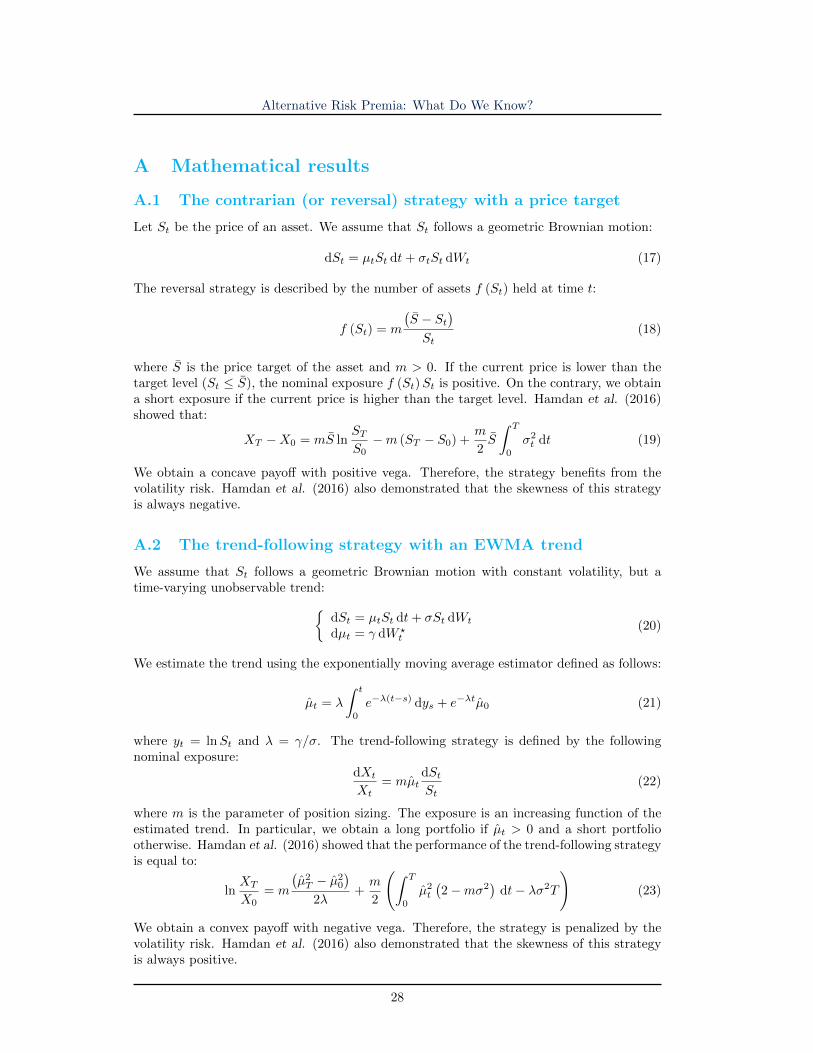
A.1 The contrarian (or reversal) strategy with a price target

Let St be the price of an asset. We assume that St follows a geometric Brownian motion:

dSt = µtSt dt+ σtSt dWt (17)

The reversal strategy is described by the number of assets f (St) held at time t:

f (St) = m

(S − St

)St

(18)

where S is the price target of the asset and m > 0. If the current price is lower than thetarget level (St ≤ S), the nominal exposure f (St)St is positive. On the contrary, we obtaina short exposure if the current price is higher than the target level. Hamdan et al. (2016)showed that:

XT −X0 = mS lnSTS0−m (ST − S0) +

m

2S

∫ T

0

σ2t dt (19)

We obtain a concave payoff with positive vega. Therefore, the strategy benefits from thevolatility risk. Hamdan et al. (2016) also demonstrated that the skewness of this strategyis always negative.

A.2 The trend-following strategy with an EWMA trend

We assume that St follows a geometric Brownian motion with constant volatility, but atime-varying unobservable trend:{

dSt = µtSt dt+ σSt dWt

dµt = γ dW ?t

(20)

We estimate the trend using the exponentially moving average estimator defined as follows:

µt = λ

∫ t

0

e−λ(t−s) dys + e−λtµ0 (21)

where yt = lnSt and λ = γ/σ. The trend-following strategy is defined by the followingnominal exposure:

dXt

Xt= mµt

dStSt

(22)

where m is the parameter of position sizing. The exposure is an increasing function of theestimated trend. In particular, we obtain a long portfolio if µt > 0 and a short portfoliootherwise. Hamdan et al. (2016) showed that the performance of the trend-following strategyis equal to:

lnXT

X0= m

(µ2T − µ2

0

)2λ

+m

2

(∫ T

0

µ2t

(2−mσ2

)dt− λσ2T

)(23)

We obtain a convex payoff with negative vega. Therefore, the strategy is penalized by thevolatility risk. Hamdan et al. (2016) also demonstrated that the skewness of this strategyis always positive.

28


A.3 Skewness aggregation of two log-normal random variables

We assume that (X1, X2) follows a bivariate log-normal distribution. This implies thatlnX1 ∼ N

(µ1, σ

21

)and lnX2 ∼ N

(µ2, σ

22

). Moreover, we note ρ the correlation between

lnX1 and lnX2. The skewness of X1 is equal to:

γ1 (X1) =e3σ2

1 − 3eσ21 + 2(

eσ21 − 1

)3/2 (24)

whereas the skewness of X1 +X2 is equal to:

γ1 (X1 +X2) =µ3 (X1 +X2)

µ3/22 (X1 +X2)

(25)

where µn (X) is the nth central moment of X. We can show that:

µ2 (X1 +X2) = µ2 (X1) + µ2 (X2) + 2 cov (X1, X2) (26)

where:

µ2 (X1) = e2µ1+σ21

(eσ

21 − 1

)(27)

and:

cov (X1, X2) = (eρσ1σ2 − 1) eµ1+ 12σ

21eµ2+ 1

2σ22 (28)

For the third moment of X1 +X2, we use the following formula:

µ3 (X1 +X2) = µ3 (X1) + µ3 (X2) + 3 (cov (X1, X1, X2) + cov (X1, X2, X2)) (29)

where:

µ3 (X1) = e2µ3+ 32σ

21

(e3σ2

1 − 3eσ21 + 2

)(30)

and:

cov (X1, X1, X2) = (eρσ1σ2 − 1) e2µ1+σ21+µ2+

σ222

(eσ

21+ρσ1σ2 + eσ

22 − 2

)(31)

A.4 A skewness model of asset returns

For modeling the skewness risk of a portfolio, Bruder et al. (2016) assume that the vectorof asset prices St = (S1,t, . . . , Sn,t) follows a jump-diffusion process:{

dSt = diag (St) dLtdLt = µdt+ Σ1/2 dWt + dZt

(32)

where µ and Σ are the vector of expected returns and the covariance matrix, Wt is a n-dimensional standard Brownian motion and Zt is the irregular component independent fromWt. More precisely, Zt =

∑Nti=1 Zi is a pure n-dimensional compound Poisson process with

a finite number of jumps, where Nt is a scalar Poisson process with constant intensityparameter λ > 0, and Z1, . . . , ZNt are vectors of i.i.d. random jump amplitudes with lawν (dz). They also assume that ν (dz) = λf (z) dz where f (z) is the probability density

function of the multivariate Gaussian distribution N(µ, Σ

), µ is the expected value of

jump amplitudes and Σ is the associated covariance matrix.

29


A.4.1 Probability distribution of asset returns

When λ is sufficiently small, we can show that asset returns33 Rt = (R1,t, . . . , Rn,t) havethe following multivariate density function:

f (y) =1− λ dt

(2π)n/2 |Σ dt|1/2

e−12 (y−µ dt)>(Σ dt)−1(y−µ dt) +

λ dt

(2π)n/2∣∣∣Σ dt+ Σ

∣∣∣1/2 e−12 (y−(µ dt+µ))>(Σ dt+Σ)

−1(y−(µ dt+µ)) (34)

It follows that it is equivalent to using a Gaussian mixture distribution for modeling assetreturns. There are two regimes:

• The ‘normal ’ regime has the probability (1− λ dt) of occurring. In this case, assetreturns are driven by the Gaussian distribution N (µdt,Σ dt).

• The ‘jump’ regime has the probability λ dt of occurring. In this case, asset returnsjump simultaneously and the jump amplitudes are driven by the Gaussian distribution

N(µ, Σ

).

We can show that the two first moments of asset returns are:

E [Rt] = µdt+ πµ (35)

and:cov (Rt) =

(Σ + λΣ

)dt+ λ (1− λ dt) µµ> dt (36)

For the skewness coefficient of Asset i, we obtain the following expression:

γ1 (Ri,t) =λ (1− λ dt)

((1− 2λ dt) µ3

i + 3µiσ2i

)dt

((σ2i + λσ2

i ) dt+ λ (1− λ dt) µ2i dt)

3/2(37)

A.4.2 Probability distribution of the portfolio’s return

Let x = (x1, . . . , xn) be the vector of weights in the portfolio satisfying∑ni=1 xi = 1. We

note Rt (x) the portfolio’s return:

Rt (x) =

n∑i=1

xiRi,t (38)

Bruder et al. (2016) show that Rt (x) has the following probability density function:

f (y) = (1− λ dt)1√

x> (Σ dt)xφ

(y − x> (µdt)√x> (Σ dt)x

)+

(λ dt)1√

x>(

Σ dt+ Σ)x

φ

y − x> (µdt+ µ)√x>(

Σ dt+ Σ)x

(39)

33The return Ri,t of asset i is defined for the holding period [t− dt, t]:

Ri,t = lnSi,t − lnSi,t−dt (33)

30


We obtain a Gaussian mixture distribution. We can show that:

E [Rt (x)] = x> (µ+ λµ) dt (40)

and:

σ (Rt (x)) =

√x>(

Σ + λΣ)xdt+ λ (1− λ dt) (x>µ)

2dt (41)

For the skewness coefficient, we obtain:

γ1 (Rt (x)) =λ (1− λ dt)

((1− 2λ dt)

(x>µ

)3+ 3

(x>µ

) (x>Σx

))dt(

x>(

Σ + λΣ)xdt+ λ (1− λ dt) (x>µ)

2dt)3/2

(42)

31

alternative risk premia: what do we know? - thierry … · alternative risk premia: what do we...

Documents