alternation on cellular automata

ELSEVIER Theoretical Computer Science 180 (1997) 229-241

Theoretical Computer Science

Alternation on cellular automata ’

Martin Matamala *

Departumento de Ingenieria Matembtica, Fact&ad de Ciencias Fisicas y Matemriticas, Universidad de Chile, Casilla 170-correo 3 Santiago, Chile

Received November 1995; revised December 1995 Communicated by E. Gales

Abstract

In this paper we consider several notions of alternation in cellular automata: non-uniform, uniform and weak alternation. We study relations among these notions and with alternating Turing machines. It is proved that the languages accepted in polynomial time by alternating Turing machines are those accepted by alternating cellular automata in polynomial time for all the proposed alternating cellular automata. In particular, this is true for the weak model where the difference between existential and universal states is omitted for all the cells except the first one. It is proved that real time alternation in cellular automata is strictly more powerful than real time alternation in Turing machines, with only one read-write tape. Moreover, it is shown

that in linear time uniform and weak models agree.

Keywords: Cellular automata; Alternation; Nondeterminism

1. Introduction

A one-dimensional cellular automata (CA) is a bi-infinite line of identical finite

machines each being in a state which is represented by a symbol taken in a finite

alphabet Q. The transition function for all finite machines is given by a function

f: Q3 + Q. The new state for a finite machine is obtained by looking its own state,

x, and the states y and z of their right and left neighbors, respectively, and then

by computing f(z,x, y). A step on the cellular automata is achieved by computing,

simultaneously, a new state for each finite machine.

A conjiguration for a CA is a function C : Z + Q which assigns to each cell an

element q in Q. Let C, be a configuration for a CA at time t. Then a configuration at

time t + 1, Ct+t , is given by

C+,(i) = f(C,(i - l),C,(i),C,(i + 1)), i E Z.

’ This work was supported under grant CEE Marie Curie ERBCISTGT 920031

* E-mail: [email protected]

0304-3975/97/$17.00 @ 1997-Elsevier Science B.V. All rights reserved PII SO304-3975(96)00214-9

230 M. Matamalal Theoretical Computer Science 180 (1997) 229-241

Cellular automata have been studied in several contexts [2,4,5,7, lo]. One of them

is to study cellular automata as language acceptors [5,9, IO]. In this sense, we consider

(U,#, Qa), where U is the input alphabet (a subset of Q), # is the quiescent state

having the quiescent property f(#, #, #) = # and Qa C Q is the set of accepting states.

Initially, an input u = uo . . .24,-l, Ui E U, i = 0,. . . , n - 1, is put in cells 0,. . . , n - 1

defining configuration Ct given by:

# i < 0 or i>n Cl(i) =

I

~~~#Uf)U, . ..U._,#.‘. 4 i E (0,. ..,n- 1) .

The input u is accepted if at some time the first cell enters an accepting state.

As for Turing machines, several generalizations can be introduced in cellular au-

tomaton models. Nondeterminism in finite automata or Turing machines gives to these

devices the possibility of multiple transitions. So, the next state (next head state, next

tape state, next move) for finite automata (Turing machine) can be chosen from a set

of possible transitions.

Nondeterminism was defined for cellular automata by Smith in [lo], where several

language complexity results were obtained. In [8], it was studied another way to in-

troduce nondeterminism on cellular automata. There, the authors relate their notion to

space and time complexity classes in Turing machines.

In model given in [lo], all the cells make an independent choice in the set of

all possible next states given by a transition function f: Q3 -+ 28. We will call that,

nonuniform model.

An nonuniform nondeterministic cellular automata (NCA) is like a CA except that

the transition function for the finite machines is a function f: Q3 + 2Q. So, a step in

NCA is achieved by choosing, independently for each finite machine, a state belongs

to f (x, y, z), where y is the state of the finite machine and, x and z are the states of

its left and right neighbors, respectively.

In the uniform version of the above definition, at each computation step some deter-

mination for f is chosen, i.e. a function f I: Q3 --) Q such that f'(x,y,z) E f(x,y,z) for every (x,~,z) E Q3 and this determination is used to update the cells.

We will see in Section 4 (Theorem 5) that the nonuniform models are at least as

much powerful than uniform ones. This result will be obtained using a synchronization

procedure.

We denote a (U)NCA, defined as above, by A = (Q, f ). Another possible nondeterministic version consists in permitting nondeterministic

transitions only in the first cell. So, we give the following definition.

A weak nondeterministic cellular automata (WNCA) is like a CA but the transition

function for cell at origin (the cell associated to position 0) is a function fo: Q --+ 2Q. We denote a WNCA by A = (Q, f, f o), where f: Q3 -+ Q is the transition function

for any cell outside the origin.

The notion of configuration for NCA, UNCA and WNCA is as for CA. If C, is a

configuration at time t of a NCA (Q, f ), then a configuration at time t + 1, Ct+i, is

M. Matamalal Theoretical Computer Science 180 (1997) 229-241 231

such that

G,l(i) E f(G(i - l), G(i), G(i + 1)).

We impose that c,+l(i) = c(+l(j) whenever ct](i-i,i,i+l) = ctl+l,j,,+il, in the case

of UNCA. This is equivalent to choose some determination f’ for f and update cells

with this determination.

For a WNCA, (Q, f, fo) the next configuration is given by

G+i(i) = .f(G(i - l), G(i), G(i + 1 I), i # 0

and

G,l(O) E fo(Ct(-l),C,(O),C,(1)).

We will prove that in polynomial time these models have the same power. This will

be a consequence of simulation results.

The results will be given in a more general framework by introducing the alternation

in cellular automata. Alternation was introduced for finite automata and later for Tur-

ing machines as models for parallel computations [3]. It consists to classify the states

(head state) of a finite automaton (Turing machine) as existential or universal ones.

An existential state, as in the nondeterministic case, is interpreted as an option in the

computation, The universal ones are associated to transitions where the device makes

two or more simultaneous actions. Since alternation is strongly related to nondetetmin-

ism we will have three kinds of alternation in cellular automata: nonuniform, uniform

and weak alternation. Other kinds of alternations could be defined but we will study

only relations between these three models. This work will focus on suitable time or

space restriction on models, so as to show where these models and Turing machines

differ or agree.

The paper is organized as follows. Section 2 is devoted to definition of alternation on

cellular automata and on Turing machine. Moreover, we define time complexity classes.

In Section 3 we give simulations of alternating cellular automata models by alternating

Turing machines (Theorem 1) and vice versa (Theorem 2). In the first case each step

in the alternating cellular automata is simulated by O(n) steps in the alternating Turing

machine, where n is the size of the current configuration in the alternating cellular

automata. In the second case, n consecutive actualizations in alternating Turing machine

are performed by 2n actualizations with a weak alternating cellular automata. Theorem

1 is a natural extension of theorems given in [lo]. Theorem 2 uses a different technique.

It consists in moving the Turing machine tape representation around the Turing machine

head representation which will be fixed at the origin cell of the cellular automata. It

is easy to see that this simulation can be extended to uniform cellular automata and

nonuniform ones. So, polynomial time restrictions are equivalent in all models.

In Section 4 we study special time restrictions: real time and linear time. In the

former, we prove that there exists a language which is recognized by a cellular automata

in real time and which is not recognized in real time by any alternating Turing machine,

with only one read-write tape.


Relations between weak and uniform models will be given, permitting to conclude

that in linear time both models agree. To complete these relations we prove that the

nonuniform model is the most powerful of all the proposed models.

2. Definitions

2.1. Alternation on cellular automata and Turing machines

An acceptor (uniform) (weak) alternating cellular automata (U)(W)ACA is a 4-

tuple d = (u,#,Qa,A) where A = (Q,J,(fo)) is a (U)(W)NCA whose states are

partitioned into existential and universal. U c Q is the input alphabet, # is the quiescent

state and Qa G Q is the set of accepting states. The (U)(W)NCA satisfies the quiescent

I= {#I

property given by

f(#, #, #) = {#I f o(#, #, #

and # cannot be created.

In order to define when an input is accepted by an (U)(W)ACA we introduce the

notion of computation tree [l]. A computation tree, T(,ol,u), for a (U)(W)ACA d

on input u, is a finite tree whose nodes are labeled by configurations and whose root

is labeled by Ci.

A computation tree for an ACA is built as follows:

Let a be a configuration with r+s nonquiescent states. Cells il, . . . , is are in existential

states and cells jl , . . . ,j, are in universal ones.

The node labeled by tx has K children labeled by configurations /?l,l,...,l, . . , ~lJQ,-.J+

where

We choose ~6 E f(c+i, aik, tlik+i ) for k = 1,. . . ,s and then we build configurations fi’,‘,..., 1,. . .) B”‘,“‘,...> n, as follows:

For every (Ii , . . . , I,), p”‘“““(ik) = a&, k = 1,. . . ,s and pl”.““‘(jk) = qf,, k = 1,. . . , Y.

So, configurations pi,‘,-.,‘, _ _ _ , pnl,n2-nr agree in sites ik and may differ in sites jk.

For WACA and UACA models the ConJigurations are divided into universal and

existential. A configuration is existential (resp. universal) when the state at origin is

existential (resp. universal).

A computation tree for WACA or UACA is a tree such that the children of any

internal node labeled by an universal (existential) configuration include all (one) of

the next configurations.

A tree T(&‘,u) is accepting if all its leaves are accepting conjgurations, i.e., con-

figurations where the state at origin belongs to Qa. We say that an ACA, UACA

or WACA & accepts u if there exists an accepting tree for & on u. The language


accepted by a (W)(U)ACA d is given by

L(.Pe) = {u/.d accepts 24},

An alternating Turing machine (ATM) is a generalization of a nondeterministic Tur-

ing machine (NTM), which is defined analogously to ACA. The states in an ATM are

divided into existential and universal ones. The definition of a configuration is slightly

different than that for CA’s: it describes the current state of the machine, the contents

of the tape (we suppose only one tape is used) and the position of the read-write head.

A new configuration is obtained by performing a step in the Turing machine, i.e., by

reading the tape symbol and, in a nondeterministic way, computing the new head state,

the new tape symbol and the next head move. A configuration is existential (universal)

if the head state is an existential (universal) one. A computation tree for an ATM M

on input u, T(M,u), is a finite tree whose nodes are labeled by configurations of M

on u, such that the root is the initial configuration and the children of any internal

node labeled by a universal (existential) configuration include all (one) of the next

configurations. The notion of accepting tree, acceptance and language accepted by A4

are analogous to those of alternating cellular automata.

2.2. Lunguages and complexity classes

We say that LY, an ATM or (W)(U)ACA, is t(n)-time bounded if for any u E L(.d)

there exists an accepting tree whose height is less than tt’juj), where ju\ is the length

of the input word u.

We define, for a (U)(W)ACA and for an ATM the following complexity classes:

(W)(U)ACA(t(n)) = {L(d)/& is a (W)(U)ACA t(n)-time bounded},

ATM(t(n)) = {L(d)/d is an ATM t(n)-time bounded}.

3. Simulating ACA in ATM

In this section, we prove that the evolution of an ACA C can be simulated by an

ATM M. A4 simulates one step of C for a configuration of size n in 3n + 5 steps.

In the first n + 1 steps, A4 moves from left to right copying the state in cell i into

cell i + 1. In the following 2(n + 2) steps, M moves from right to left making the

actualization of all the cells.

Theorem 1. Let C be an ACA. Then there exists an ATM M such that L(C) =

L(M). If C has time complexity t(n) then M has time complexity O(t2(n)).

Proof. The simulation of one step of C can be done through 3n + 5 steps of M. Set

!&=Qcx{R,LH}U{ > h w w ere w is the accepting state, and the alphabet

4~ = 4?c u <Qc x {*)I u Q:: u <Q$ x {*)I.


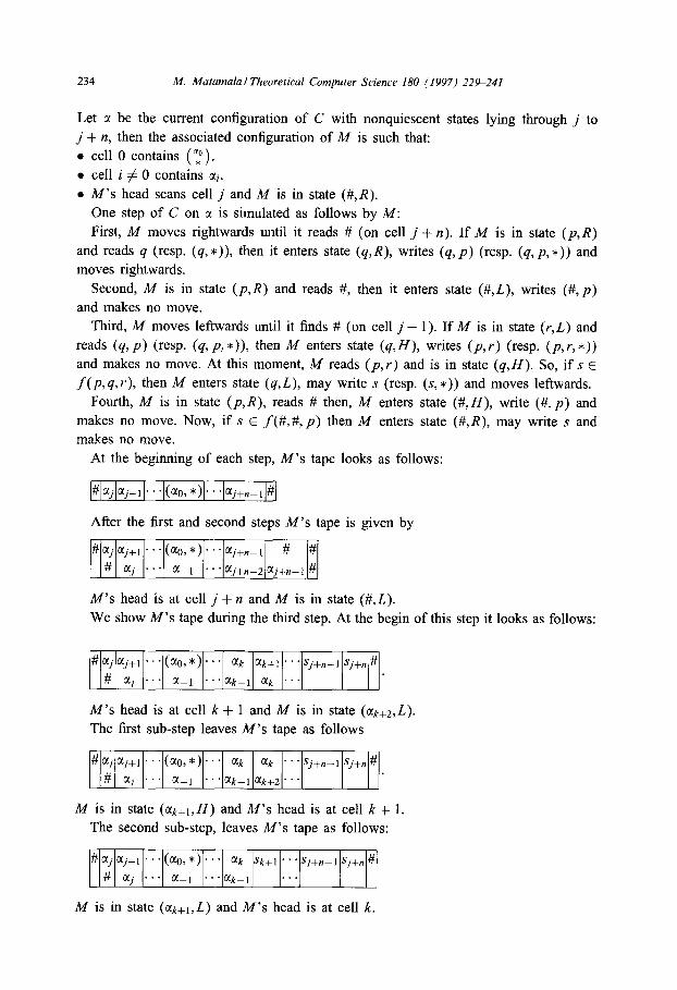
Let c( be the current configuration of C with nonquiescent states lying through j to

j + n, then the associated configuration of A4 is such that:

0 cell 0 contains (“*“).

0 cell i # 0 contains ai.

l M’s head scans cell j and A4 is in state (#,R).

One step of C on a is simulated as follows by M:

First, M moves rightwards until it reads # (on cell j + n). If M is in state (p,R)

and reads q (resp. (q, *)), then it enters state (q,R), writes (q, p) (resp. (q, p, *)) and

moves rightwards.

Second, M is in state (p,R) and reads #, then it enters state (#,L), writes (#, p)

and makes no move.

Third, M moves leftwards until it finds # (on cell j - 1). If M is in state (r,L) and

reads (q, p) (resp. (q, p, *)), then M enters state (q,H), writes (p, r) (resp. (p, r, *))

and makes no move. At this moment, M reads (p, r) and is in state (q,H). So, if s E

f(p,q,r), then M enters state (q,L), may write s (resp. (s, *)) and moves leftwards.

Fourth, M is in state (p,R), reads # then, M enters state (#, H), write (#, p) and

makes no move. Now, if s E f(#, #, p) then M enters state (#,R), may write s and

makes no move.

At the beginning of each step, M’s tape looks as follows:

I#lajlaj+ll.. #ao, *)I. * -IC(i+n_ll#

After the first and second steps M’s tape is given by

#cljoLj+l -..(a~,*)...CCj+~-l # # # OIj ... a-1 ... oIj+,_2 aj+-l#

M’s head is at cell j + n and M is in state (#,L).

We show M’s tape during the third step. At the begin of this step it looks as follows:

# aj aj+i . . . (a0, *) ’ . . ak ak+l . . . Sj+,-1 Sj+n #

# aj .” a-1 “‘ak__l ak . . .

M’s head is at cell k + 1 and M is in state (ak+&L).

The first sub-step leaves M’s tape as follows

8 aj aj+i ’ (a0, *) . . . ak ak . . . Sj+,-1 Sj+n #

# aj ‘.’ a-1 “‘ak__lak+2”’

M is in state (ak+i,H) and M’s head is at cell k + 1.

The second sub-step, leaves M’s tape as follows:

# Uj aj+l . . (ao, *) . . ak Sk+1 . . ’ Sj+,_l Sj+n #

# aj ... a-1 “‘&-_I ...

M is in state (ak+l ,L) and M’s head is at cell k.

M. Matamalai Theoretical Computer Science 180 (1997) 229-241 235

The simulation finishes when A4 finds the symbol #. At this time M’s tape looks as

follows:

A4 is in state (#,R) and M’s head is at cell j - 1.

The simulation of one transition of C takes (n + 1) + 2(n + 2) = 3n + 5 steps, then

we get the quadratic bound:

States of the form (q,H) will be existential if q is existential (resp. are universal if

q is universal). Other states lead to deterministic moves.

Now, since accepting configurations in C were defined as having an accepting state

in the origin, the accepting state w is entered in M’s head when a state (8) appears

in the origin, with q an accepting state. 0

Now, we want to give the inverse result, i.e., we want to simulate the behavior

of an ATM into an ACA. Next theorem shows how to simulate the evolution of an

ATM into a WACA. We could make it by associating a pair (z) to the scanned

symbol and leave unchanged the other cells position. Since M could make nonde-

terministic transitions in any position, the WACA should go at the first position to

make the simulation of M’s transition and then came back to the position where M’s

head should move. This solution is ‘sequential’ like and we should obtain a simulation

of M’s evolution in quadratic time. We can improve this result with a more parallel

solution.

Theorem 2. Let M be an ATM. Then there exists a WACA C accepting L(M). IJ

M has t(n)-time complexity then C has 2t(n)-time complexity.

Proof. The idea is to move M’s tape around the origin. M’s head will always be at

origin represented by vector states n

0 4 where a E (0, 1) is a control character, 4 is

the state of M and cr is the symbol slanned by M. When M moves right (resp. left)

two families of signal, (‘f ) and (‘f ) (resp. ( “> and (If) ) are produced moving M’s

head representation one position to the left (resp. right) of the origin. Signals (‘p) and

( > ‘” move rightwards while signals (‘f) and ‘f; move leftwards.

( ) Before giving formal proof we show in an example how the simulation evolves.

Suppose the evolution on M is

# a0 a1 . ..an_.# v

+ #ah rJ’1 cT2...(T,_,# 4cJ;o; 02 g3...fJn-,#+ v v

40 4 4;

+ #ah ai 0:. . .a,-,#+ # ah ay...a,_t# V V

4; 9;’

236 M. Matamala J Theoreiicaf Curnputer Science 180 (1997) 229-241

These steps are simulated in C by

# #

# #

# #

# #

# #

# 00 01 62 Q3

0

# 0

00 01 62 (73

40

# # (2) (;$ (z) (T3 (;) ‘76 (;I”) #

# (f) # (p1) df (I) (74 (it) # #

and signal evolutions are given by


when M’s transition is (q,c) -+ (q’,c’, I) and

when M’s transition is (q,c) -+ (q’,c’,r). Here, symbol ? at position i signifies that

the information to update site i is incompleted.

Let (ql,yf,il) be the configuration at time t for M. It can be proved, by induction

on t that:

w>o 0

. c*‘+‘(o) = qr

0

l yj> lC?‘+Iqj) = ‘l;,+i

Y:, l M moves right at time t then Vj 2 2

Yi,-j+l Yi,-j+l # #

otherwise

0 kt moves left at time t then vj’jb2

C 2f+2+jl{_j_l,_j) =

d-j-1 d-j-1 # # otherwise

Therefore, each transition in M is simulated by two steps in C.


States 0

L are existential (resp. universal) when q is existential (resp. universal). 9

All other states are deterministic. Moreover,

Q:, = /q accepting state for M

So, any accepting computation tree for M on u has associated an accepting computation

tree of C on u with twice its height. 0

Remark 1. For UACA and for ACA we can make an analogous construction ob-

taining real time simulations. It is due to the fact that UACA and ACA can make

nondeterministic transition in any cell.

Previous results prove that polynomial time languages for (W)(U)ACA and ATM

agree. This fact came from polynomial simulation of these models.

Now, we analyze another time restrictions: linear and real time.

4. Real and linear time on ATM and ACA

4.1. rATMcrACA

In this subsection, we prove that there exists a Ianguage recognized in real time by

a deterministic CA and which is not recognized by an ATM in real time.

This language is the palindrome set defined by

~={w~U*/w=w’}, wherew=wiw2...wn andw’=w,...w2wi.

Proposition 1. 9 E rCA and P 4 rATM.

Proof. The former affirmation is proved in [5] for cellular automaton where the input

is put step by step in the first cell and later in [lo] it was proved also for the cellular

automata defined like those defined here.

In order to prove the second affirmation we observe that if there were an ATM

accepting 9 it should read all its inputs to give any answer. So, since we want to

make it in real time the machine at time i reads the ith position and moves right.

Since the machine cannot read symbols already read then it has to works like a finite

automata. In [3,6] it is proved that the power of a finite automata, nondeterministic

finite automata and alternating finite automata are the same when they work as language

recognizers. Furthermore, it is known that 22’ is not a regular language which concludes

the proof. 0

Corollary. rATM c rACA.

M. Matamalal Theoretical Computer Science I80 (1997) 229-241 239

Proof. Since CA(t(n)) &ACA(t(n)) from Proposition 1 we get that 9 E rACA. From

Remark 1 we know that rATM 5 rACA and so the result holds. q

4.2. Linear time in ACA

In this subsection, we prove that UACA and WACA agree in linear time. For that we

prove two theorems which execute the simulation of UACA by WACA and reciprocally

of WACA by UACA.

Theorem 3. Let C be a WACA. Then, there exists a UACA C’ such that L(C) = L(C’). If C is t(n)-time bounded then C’ is t(n)-time bounded.

Proof. Let J‘, fo and Q be the transition functions and the state set for C. We define

the transition function for C’ g as f in states which belong to Q and as f. in states

which belong to {*} x Q.

Let T(C,u) be a computation tree for C on u. We build a computation tree, T(C’, u) for C’ on u, which is accepting if and only if T(C, u) is accepting. Let a a configuration

in T(C, u). We associate in T(C’, u) a configuration @(a) given by

@(a): . ..a_.... * ( > c(, . ..q..

UO

It is easy to see that the children for @(c() in T(C’,u) are @(p’) where p’ are the

children of CI in T(C, u) 0

Theorem 4. Let C be an UACA. Then there exists a WACA C’ such that L(C) =

L(C’). If C is t(n)-time bounded then C’ is 0(2t(n)) time bounded.

Proof. Let T(C,u) be an accepting tree for u. Let p be its height. We build an

accepting tree T(C’, u) for u of height 2p. Let qh, h 3 1 a configuration labeling a

node in T(C, u), at level h, let ei, e2, . , eh be the choices leading from the root to czh

and .‘,EI ,..., ~8 the configurations labeling the path in T(C, u) defined by the choices

el,. . . ,eh. We associates to fxh a configuration in T(C’,u), @ = @(ah,crh-‘, ,cz”,

eh,...,eo) given by

The transition in C’ transforms @ into @’ given by

240 M. Matamalai Theoretical Computer Science 180 (1997) 229-241

States (i) are existential for C’ if and only if u is existential for C (universal other-

wise). So, when E; is an existential state, &h will have only one child in T(C,u), ah+’

which is obtained by updating c? via some determination of f. In this case @(ah) will

have @‘(ah) as the only child and eh+l gives the determination chosen by C. Then

updating once more C’ we obtain a configuration @“(ah), which is equal to @(czh+l).

When ~1 is an universal state, @h will have as children all the configurations obtained

from gh by applying some determination off. So, @(ah) will have as children all the

configurations Qji< ah) given by

@j(Mh) : ” ’ (d$) ( iF21) (a (;;) (2 ( 4) (a8 -2 a2

where j E {1,2,. . . ,K} and K = niEej If(i 0

Corollary. 1 UACA = 1 WACA.

Proof. Since O(2n) = O(n) the proof comes directly from the last theorems. 0

Theorem 5. UACA(t(n)) &AC4 (t(n)).

Proof. Let C be an UACA given by (Q, f, U, Qa, #). Let C’ = (Q’, g, U, QL, #) be the

ACA simulating C. We take Q’ = (0, 1, . . . , K} x Q U Q where K is the number of

possible determinations for f. We define the maps (pi, i = 1,2. qp’ is defined from Q’

into Q. It is the identity function over Q and is the second projection over the set

(031,. . ., K} x Q. (p2 is the first projection over the set (0, 1, . . . , K} x Q and is defined

as 1 over Q. Function g is defined as follows:

cj = fj(t#?(u), 4’(v), #l(w)>, j = 1,. . . ,K}

if +2(u) = 952(u) = 42(w) # 0,

otherwise.

So, at time t31 the nonquiescent part of a configuration for C’ will be 0

‘: c; ’

. ..> 0 4 c: .

Let C’ be an accepting configuration for C on u at time t. Since acceptance is

defined in the cell at origin, C’ must be sure that its accepting configurations are only

those obtained by uniform elections on cell that may modify the values of cell at origin

at time t. At time s < t, these cells are those belonging to {-(t - s), . . . , (t - s)}. It is

easy to see, by induction on t that if ef is the value of the first coordinate (for these

cells being in a non-quiescent state) of the ith cell at time t then ef # 0 if and only if

M. Maramalal Theoretical Computer Science 180 (1997) 229-241 241

Vl <I’ <t t7’j E {i - (t - t’), i + t - t’} e$’ = e:‘. So, accepting trees for C on u have

associated at least one accepting tree for C’ on U.

5. Conclusion

It was proved that alternating cellular automata and alternating Turing machine have

the same power when there are no restrictions in the sources. This is true even when

polynomial restriction is made on the time. This is no longer true when we considered

real time since we can then separate the class defined by alternating cellular automata

and alternating Turing machine.

We observe that all the results obtained here apply to the nondeterministic case when

we consider only existential states.

From Theorems 1, 2 and 3 we have seen that general alternation in cellular automata

is as powerful as weak alternation when we consider the polynomial time class. This

could be interesting for simulation of alternation, in particular random simulation, be-

cause our result says that if simulation time is reasonably larger (polynomial), then one

can make random choices only in the first position and still obtain the same language

complexity.

References

[I] J.L. BalcBzar, _I. Diaz and J.Gabarr6. Structural Complexity II, EATCS monograph Series, Vol. 22

(Springer, Berlin, 1990).

[2] W. Bucher and K. Culik II, On real time and linear time cellular automata, RAIRO Inform. Theor. 18 (4) (1984) 307-325.

[3] A.K. Chandra, D.C. Kozen and L.J. Stockmeyer, Alternation, J. ACM 28 (1981) 114-133.

[4] J.H. Changa, O.H. Ibarra and A. Vergis, On the power of one-way communication. J. ACM 35 (3) (I 988) 697-726.

[S] S.N. Cole, Real-time computation by n-dimensional iterative arrays of finite-state machines, IEEE Trans

comput. cl8 (14) (1969) 349-365.

[6] J.E. Hopcroti and J.D. Ullman, Introduction to Automata theory, Languages and Compuration (Addison-Wesley, Reading, MA, 1979).

[7] 0. Ibarra and T. Jiang, On one-way cellular arrays, SIAM J. Comput. 16 (6) (1987) 1135-I 154.

[8] K. Krithivasan and M. Mahajan. Nondeterministic, probabilistic and alternating computations on

cellular array models, preprint, Department of Computer Science and Engineering, lndian Institute of

Technology, Madras 600 036, India.

[9] J. Mazoyer and N. Reimen, A linear speed-up theorem for cellular automata, Theoret. Comput. Sci 101 (1992) 59-98.

[lo] A.R. Smith Ill, Real-time language recognition by one-dimensional cellular automata, J. Compur. System Sci. 6 (1972) 223-253.

alternation on cellular automata

Documents