almost robust optimization with binary variables robust... · almost robust optimization with...

Almost Robust Optimization with Binary Variables

Opher Baron, Oded Berman, Mohammad M. Fazel-ZarandiRotman School of Management, University of Toronto, Toronto, Ontario M5S 3E6, Canada,

[email protected], [email protected], [email protected]

Abstract

The main goal of this paper is to develop a simple and tractable methodology (boththeoretical and computational) for incorporating data uncertainty into optimizationproblems in general and into discrete (binary decision variables) optimization prob-lems in particular. We present the Almost Robust Optimization (ARO) model thataddresses data uncertainty for discrete optimization models. The ARO model trade-offs the objective function value with robustness, to find optimal solutions that arealmost robust (feasible under most realizations). The proposed model is attractive dueto its simple structure, its ability to model dependence among uncertain parameters,and its ability to incorporate the decision maker’s attitude towards risk by controllingthe degree of conservatism of the optimal solution. Specifically, we define the Robust-ness Index that enables the decision maker to adjust the ARO to better suit her riskpreference. We also demonstrate the potential advantages of being almost robust asopposed to being fully robust. To solve the ARO model with discrete decision vari-ables efficiently, we develop a decomposition approach that decomposes the model intoa deterministic master problem and a single subproblem that checks the master prob-lem solution under different realizations and generates cuts if needed. Computationalexperiments demonstrate that the decomposition approach is able to find the optimalsolutions up to three orders-of-magnitude faster than the original formulation. Wedemonstrate our methodology on the knapsack problem with uncertain weights, thecapacitated facility location problem with uncertain demands, and the vehicle routingproblem with uncertain demands and travel times.

1. Introduction

Binary requirements on decision variables are essential in many operational and planning

models. A variety of applications with such requirements include: facility location, vehicle

routing, production planning and scheduling. Traditional optimization models for these

1

applications assume that the parameters and data are known and certain. In practice,

however, such assumptions are often unrealistic, e.g., the data may be noisy or incomplete.

Two of the main approaches used to incorporate uncertainty are stochastic program-

ming (see Ruszczynski and Shapiro (2003) and references therein) and chance constrained

programming (Charnes and Cooper (1959)). In stochastic programming (which are usu-

ally modeled in two stages) the decision maker optimizes an expected value of an objective

function that involves random parameters. In the Chance Constrained Programming, the

decision maker wants to ensure that the constraints hold with at least a specified level of

probability. Both approaches are typically not effective when the inclusion of discrete deci-

sion variables is required, then these problem becomes very challenging to solve.

Another approach to handle uncertainty is robust mathematical programming, Mulvey

et al. (1995), which presents an approach that integrates goal programming formulations

with scenario-based description of the problem data. The approach seeks to generate so-

lutions that are less sensitive to the specific realization of the data. Mulvey et al. (1995)

only consider convex optimization models and compare the advantages of their model to

parameter sensitivity analysis and to solutions obtained from stochastic programming.

Another method to incorporate uncertainty into optimization problems is robust op-

timization. Unlike stochastic programming, chance constrained programming, and robust

mathematical programming that use probabilistic information, in robust optimization the

uncertainty is set-based, requiring no specific information about the distribution functions.

In such models, the decision-maker seeks to find solutions that are feasible for any realiza-

tion of the uncertainty in a given set (see Ben-Tal and Nemirovski (1998, 1999, 2000, 2001),

El-Ghaoui et al. (1998), Bertsimas and Sim (2004), Chen et al. (2007), Natarajan et al.

(2008)). The majority of these papers, however, focus on convex optimization and limited

work is done on discrete optimization problems (exceptions include: Kouvelis and Yu (1997),

Averbakh (2001), Bertsimas and Sim (2003), Atamturk (2006), Atamturk and Zhang (2007),

and Baron et al. (2011)).

In this paper, we present the Almost Robust Optimization (ARO) model that incorpo-

rates data uncertainty, into optimization models. The ARO, trade-offs the objective function

value with robustness of the solution (robustness is measured by the amount of violation of

2

the uncertain constraints under different realizations) to find optimal solutions that are al-

most robust (feasible for most data realizations). The ARO also incorporates the decision

maker’s attitude towards risk (control over the degree of conservatism of the optimal solution

and the degree of the robustness of the solution). An important advantage of our model is

its tractability for problems with discrete (binary) decision variables. Thus, our exposition

is focused on such problems, modeling the data uncertainty using a set of scenarios. But our

model can also be utilized for optimization problems with general uncertainty sets.

The ARO approach combines ideas from stochastic programming, chance constrained

programming, robust mathematical programming, and robust optimization. A comparison

of these approaches with ARO is presented in Table 1 and further discussed below.

• Robust optimization vs. ARO: Both robust optimization and ARO seek to find solu-

tions that are robust given an uncertainty set and can incorporate the decision makers’

risk attitude (Bertsimas and Sim (2004), Natarajan et al. (2009), and Ben-Tal et al.

(2010)); there are two main differences between them. First, unlike robust optimiza-

tion, ARO can use probabilistic knowledge of the uncertain data. In particular, ARO

can be setup to suit a wide spectrum of available probabilistic information such as:

full probabilistic information, no probabilistic information, and partial probabilistic

information. Second, in robust optimization the constraints are usually hard, i.e., the

constraints must be satisfied for all possible realizations of the data, (exceptions in-

clude Ben-Tal et al. (2006) and Ben-Tal et al. (2010))) while in ARO, both hard and

soft constraints can be accommodated, i.e., the decision maker has the choice to de-

cide whether or not to allow infeasibility under some realizations. Note that even the

framework of generalized robust optimization that allows large data variations, which

can be thought of as rare scenarios, treats the constraints as hard (see chapter 3 of

Ben-Tal et al. (2009)).

• Stochastic programming vs. ARO: The main similarity between the two models is that

they use probabilistic knowledge of the uncertain parameters; but ARO also applies to

situations with limited probabilistic information. The main difference is that stochastic

programming models seek to minimize the expected cost (dis-utility) of a decision made

3

in the first stage, while ARO seeks to find solutions that are almost robust (feasible

under most realizations). Furthermore, unlike ARO which accommodates both hard

and soft constraints, stochastic programming only considers soft constraints. Finally,

while discrete variables can make stochastic programming hard and computationally

intractable, the discrete variable version of the ARO (as will be discussed shortly) is

much more tractable.

• Chance constrained programming vs. ARO: As we show in Section 2.2, chance con-

straints are a special case of ARO. Conceptually, however, there are two main difference

between these models: first, we believe that the ARO is more suitable for cases where

the decision maker faces quantitative risk (i.e., cases where measuring the amount of

constraint violation is important), whereas chance-contraints are more suited for cases

with qualitative risk (i.e., cases where instead of the amount of violation, including

violation with its probability is important); secondly, while chance constraints require

probabilistic knowledge of the uncertain parameters, ARO can be applied to setting

with limited (or no) probabilistic information.

• Robust mathematical programming vs. ARO: The ARO retains the advantages of ro-

bust mathematical programming while offering the following additional advantages:

first, ARO allows control of the degree of conservatism for every constraint (i.e., gives

the decision maker control over the amount of violation allowed for each uncertain con-

straint), thus, fully integrating the decision makers’ risk attitude in the optimization

model. Second, while robust mathematical programming only considers a scenario-

based description of the uncertain data, the ARO can also address general uncertainty

structures. Third, while robust mathematical programming assumes that the prob-

ability distribution of the scenarios are known, ARO can also be used for setting in

which the probabilistic information of the uncertain data is limited. Finally, while ro-

bust mathematical programming focuses on convex optimization, we focus on discrete

optimization models. This generalization makes the problems much more difficult to

solve and thus the issue of tractability arises. To overcome this issue, we develop a

tractable decomposition approach for solving such problems.

4

Model Constraint Uncertainty Incorporate RiskType Type Risk Type

Stochastic Programming Soft Probabilistic Indirectly QuantitativeChance Constrained Programming Soft / Hard Probabilistic Directly QualitativeRobust Mathematical Programming Soft Probabilistic Indirectly QuantitativeRobust Programming Usually Hard Non-Probabilistic Directly QualitativeARO Soft / Hard Probabilistic / Directly Quantitative

Non-Probabilistic (accommodates Qualitative)

Table 1: Comparison of ARO with Other Approaches.

The main goal of this paper is to develop a simple, practical, and tractable methodol-

ogy for incorporating data uncertainty into discrete optimization problems. Therefore, the

exposition is focused on the discrete optimization version of the ARO, which we refer to as

the Almost Robust Discrete Optimization model (ARDO).

Due to both its combinatorial and uncertain nature, ARDO can be difficult to solve.

To overcome such difficulties, we develop a decomposition approach, in which the ARDO

is decomposed into a deterministic master problem and a single subproblem which checks

the master problem solution under different realizations and generates cuts if needed. Our

computational experiments demonstrate that the decomposition approach is very effective,

i.e., it is able to find an optimal solution up to three orders-of-magnitude faster than the orig-

inal formulation. Furthermore, unlike the original formulation, in which the computational

difficulty drastically increases with the number of scenarios, the number of scenarios does

not substantially affect the computational difficulty of the decomposition approach. Another

important upside of our approach is that since the master problem is a deterministic discrete

optimization problem, existing approaches for solving such problems can be incorporated into

the decomposition model to speed up the solution procedure. Our decomposition approach

also overcomes the main drawbacks of the integer L-shape method (Laporte and Louveaux

(1993)), which is the main tool used to solve stochastic integer programs. Specifically, unlike

the L-shaped method, in which the subproblems are integer programs and are hard to solve,

the subproblem in our model is very simple to solve; furthermore, in the integer L-shape

method, the cuts are generated from the relaxed LP dual of the subproblems (this relax-

ation can substantially decreases the efficiency of the approach), while our cuts are uniquely

designed for integer programs.

In summary, the main contributions of this paper are threefold. First, we introduce

5

the Almost Robust Optimization model and formulation that is simple, intuitive, flexible,

and easy to communicate to managers. This formulation allows uncertainty in the decision

making process and bridges stochastic programming and robust optimization. Second, we

develop a decomposition approach to efficiently solve the Almost Robust Optimization model

with discrete (binary) decision variables. We show that our methodology is practical and

computationally tractable for discrete optimization problems that are subject to uncertainty.

Third, by defining the Robustness Index we demonstrate the potential advantages of being

almost robust as opposed to being fully robust.

The paper is organized as follows. Section 2 presents the general framework and formu-

lation of the ARO. The details of the decomposition approach are described in Section 3.

Some applications are provided in Section 4. Computational results are presented in Section

5. Section 6 concludes the paper. Proofs and extensions are included in the Appendices.

2. Almost Robust Optimization

In this section, we present models that incorporate data uncertainty in the decision making

process using a scenario-based description of the data (as we demonstrate in Section 6, our

approach also works when the uncertainty has other structures). Scenarios are used since

they are very powerful, convenient and practical in representing uncertainty, and they allow

the decision maker considerable flexibility in the specification of uncertainty (e.g., uncertain

data may be highly correlated, may be samples from simulation, and/or may be obtained

from historical data).

This section is divided into two parts. We first present some prior formulations in which

scenario-based data are incrementally incorporated into a deterministic optimization model,

and discuss their advantages and disadvantages. Then, we present our Almost Robust Op-

timization model.

2.1 Prior Optimization Models

Deterministic Model: Consider a deterministic optimization problem of the form

6

min z = cTxs.t. Ax ≤ b , (Deterministic Model)

x ∈ X,

where x, c, and b are N × 1 vectors and A is a (M + J)×N matrix.

The classical paradigm in mathematical programming assumes that the input data of the

above formulation is known. In practice, however, portions of the data may be uncertain.

Without loss of generality, we assume that the data uncertainty affects only a partition of

A. As is standard (see Ben-Tal et al. (2009)), we assume that both c and b are deterministic.

(These can be achieved by incorporating them into the uncertain partition of A, by adding

the constraint z − cTx ≤ 0, introducing a new variables 1 ≤ xn+1 ≤ 1, and transforming the

constraints to Ax − bxn+1 ≤ 0.) We discuss a treatment on uncertain objectives in a more

general manner in Section 2.2. We partition A into a deterministic M ×N matrix, D, and

an uncertain J × N matrix U . Similarly, we partition the vector b into a M × 1 vector bD

corresponding to the deterministic partition of A, and a J × 1 vector bU corresponding to

the uncertain partition.

As discussed in the introduction, we focus on discrete optimization problems in which

x ∈ X ⊆ 0, 1N . Such problems are often difficult to solve due to the their integrality

and combinatorial nature, and indeed many of them are NP-hard. In particular, convexity,

which often exists in problems with continuous variables, no longer holds in problems with

integrality constraints. For a comprehensive discussion of the theory of optimization prob-

lems with integrality constraints, and the general tools developed for solving them efficiently

see Nemhauser and Wolsey (1988), Wolsey (1998), and Bertsimas and Weismantel (2005).

As stated earlier, in the body of the paper (except in Section 6) we assume that the

uncertain data is represented by a set of scenarios S = 1, 2, ..., |S|, with probabilities ps

for each s ∈ S. Each scenario is associated with a particular realization of the uncertain

matrix, U s with corresponding entries usij. Note that later in this section, we show that our

Almost Robust Optimization model can also be setup to suit a wide spectrum of available

probabilistic information such as: full probabilistic information, no probabilistic information,

and partial probabilistic information.

7

We next introduce two existing models that incorporate scenarios into the deterministic

model and discuss their advantages and disadvantages.

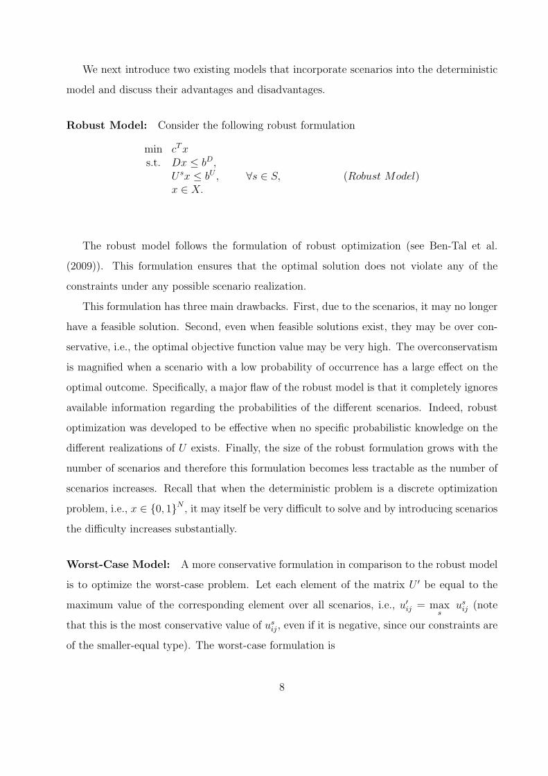
Robust Model: Consider the following robust formulation

min cTxs.t. Dx ≤ bD,

U sx ≤ bU , ∀s ∈ S, (Robust Model)x ∈ X.

The robust model follows the formulation of robust optimization (see Ben-Tal et al.

(2009)). This formulation ensures that the optimal solution does not violate any of the

constraints under any possible scenario realization.

This formulation has three main drawbacks. First, due to the scenarios, it may no longer

have a feasible solution. Second, even when feasible solutions exist, they may be over con-

servative, i.e., the optimal objective function value may be very high. The overconservatism

is magnified when a scenario with a low probability of occurrence has a large effect on the

optimal outcome. Specifically, a major flaw of the robust model is that it completely ignores

available information regarding the probabilities of the different scenarios. Indeed, robust

optimization was developed to be effective when no specific probabilistic knowledge on the

different realizations of U exists. Finally, the size of the robust formulation grows with the

number of scenarios and therefore this formulation becomes less tractable as the number of

scenarios increases. Recall that when the deterministic problem is a discrete optimization

problem, i.e., x ∈ 0, 1N , it may itself be very difficult to solve and by introducing scenarios

the difficulty increases substantially.

Worst-Case Model: A more conservative formulation in comparison to the robust model

is to optimize the worst-case problem. Let each element of the matrix U ′ be equal to the

maximum value of the corresponding element over all scenarios, i.e., u′ij = max

susij (note

that this is the most conservative value of usij, even if it is negative, since our constraints are

of the smaller-equal type). The worst-case formulation is

8


U ′x ≤ bU , (Worst− Case Model)x ∈ X.

As can be seen, the worst-case model, which is a special case of Soyster (1973) in which

uncertain matrix belong to a convex set of scenarios, has all the drawbacks of the robust

model (its solution is even more conservative). The main upside of this model compared to

the robust model is its smaller size that makes it more tractable in general (its complexity

is the same as that of the deterministic model independent of the number of scenarios).

2.2 The Almost Robust Optimization Model

We next introduce a model that overcomes the issues of infeasibility and overconservatism,

and which integrates the decision maker’s risk attitude into the optimization process. This

model, which we refer to as the Almost Robust Optimization (ARO) model trade-offs the

solution value with robustness to find solutions that are almost robust (feasible under most

realizations). In such a model infeasibility of the uncertain constraints under some of the

scenarios may be allowed at a penalty.

Consider the jth uncertain constraint, U sj x ≤ bUj . For every j ∈ 1, .., J , the amount of

infeasibility of solution x in scenario s can be measured by

Qsj(x) = max0, (U s

j x− bUj ) ≡ (U sj x− bUj )

+, (1).

Our approach allows other measures of infeasibility such as the absolute value of in-

feasibility, Qsj(x) = |U s

j x − bUj |, which is applicable for equality constraints. In the body

of the paper, we focus on the infeasibility measure (1), and defer the explanation of the

incorporation of the absolute value measure to Appendix C.

We now introduce penalty functions to penalize uncertain constraint violations. Three

alternative penalty functions (based on the available probabilistic information) are:

• Expected Penalty Function: this penalty function is suitable for situations where the

decision maker has full probabilistic knowledge of the scenarios. This penalty function

has the form:

9

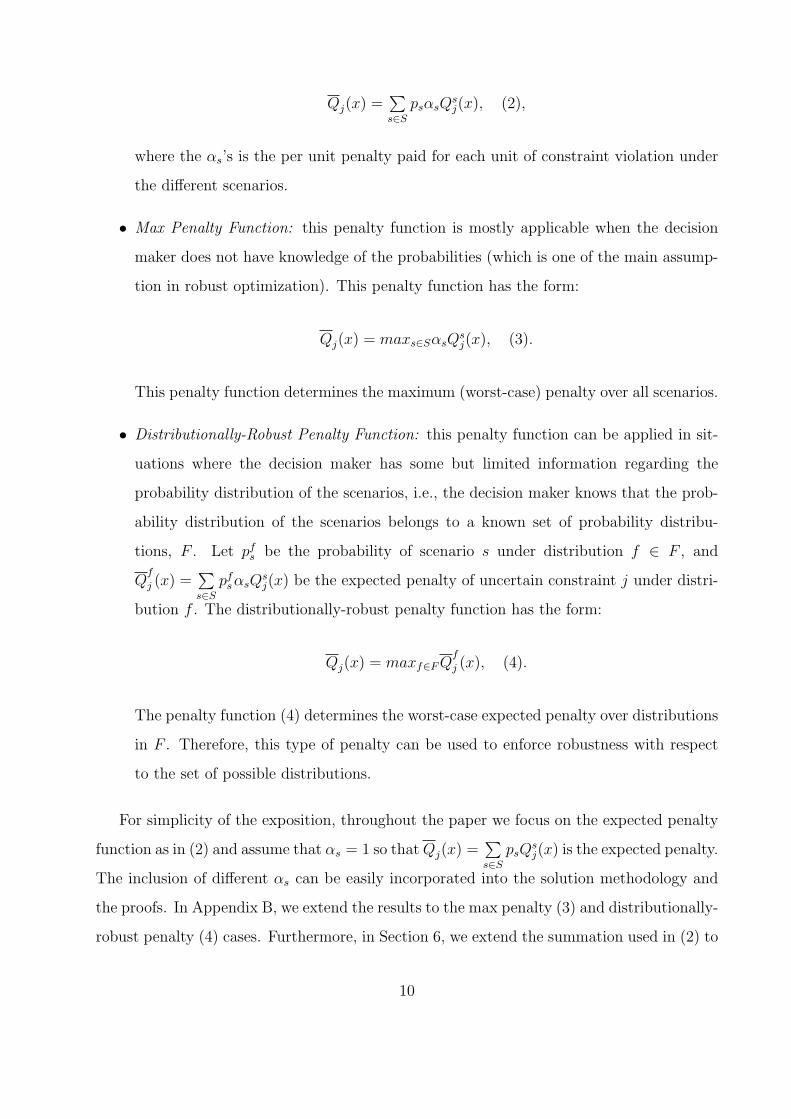
Qj(x) =∑s∈S

psαsQsj(x), (2),

where the αs’s is the per unit penalty paid for each unit of constraint violation under

the different scenarios.

• Max Penalty Function: this penalty function is mostly applicable when the decision

maker does not have knowledge of the probabilities (which is one of the main assump-

tion in robust optimization). This penalty function has the form:

Qj(x) = maxs∈SαsQsj(x), (3).

This penalty function determines the maximum (worst-case) penalty over all scenarios.

• Distributionally-Robust Penalty Function: this penalty function can be applied in sit-

uations where the decision maker has some but limited information regarding the

probability distribution of the scenarios, i.e., the decision maker knows that the prob-

ability distribution of the scenarios belongs to a known set of probability distribu-

tions, F . Let pfs be the probability of scenario s under distribution f ∈ F , and

Qf

j (x) =∑s∈S

pfsαsQsj(x) be the expected penalty of uncertain constraint j under distri-

bution f . The distributionally-robust penalty function has the form:

Qj(x) = maxf∈FQf

j (x), (4).

The penalty function (4) determines the worst-case expected penalty over distributions

in F . Therefore, this type of penalty can be used to enforce robustness with respect

to the set of possible distributions.

For simplicity of the exposition, throughout the paper we focus on the expected penalty

function as in (2) and assume that αs = 1 so thatQj(x) =∑s∈S

psQsj(x) is the expected penalty.

The inclusion of different αs can be easily incorporated into the solution methodology and

the proofs. In Appendix B, we extend the results to the max penalty (3) and distributionally-

robust penalty (4) cases. Furthermore, in Section 6, we extend the summation used in (2) to

10

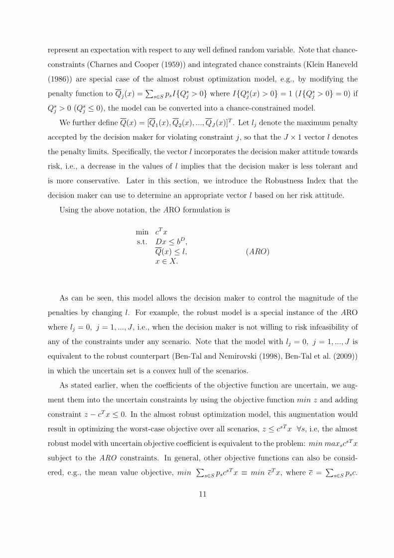
represent an expectation with respect to any well defined random variable. Note that chance-

constraints (Charnes and Cooper (1959)) and integrated chance constraints (Klein Haneveld

(1986)) are special case of the almost robust optimization model, e.g., by modifying the

penalty function to Qj(x) =∑

s∈S psIQsj > 0 where IQs

j(x) > 0 = 1 (IQsj > 0 = 0) if

Qsj > 0 (Qs

j ≤ 0), the model can be converted into a chance-constrained model.

We further define Q(x) = [Q1(x), Q2(x), ..., QJ(x)]T . Let lj denote the maximum penalty

accepted by the decision maker for violating constraint j, so that the J × 1 vector l denotes

the penalty limits. Specifically, the vector l incorporates the decision maker attitude towards

risk, i.e., a decrease in the values of l implies that the decision maker is less tolerant and

is more conservative. Later in this section, we introduce the Robustness Index that the

decision maker can use to determine an appropriate vector l based on her risk attitude.

Using the above notation, the ARO formulation is


Q(x) ≤ l, (ARO)x ∈ X.

As can be seen, this model allows the decision maker to control the magnitude of the

penalties by changing l. For example, the robust model is a special instance of the ARO

where lj = 0, j = 1, ..., J , i.e., when the decision maker is not willing to risk infeasibility of

any of the constraints under any scenario. Note that the model with lj = 0, j = 1, ..., J is

equivalent to the robust counterpart (Ben-Tal and Nemirovski (1998), Ben-Tal et al. (2009))

in which the uncertain set is a convex hull of the scenarios.

As stated earlier, when the coefficients of the objective function are uncertain, we aug-

ment them into the uncertain constraints by using the objective function min z and adding

constraint z − cTx ≤ 0. In the almost robust optimization model, this augmentation would

result in optimizing the worst-case objective over all scenarios, z ≤ csTx ∀s, i.e, the almost

robust model with uncertain objective coefficient is equivalent to the problem: min maxscsTx

subject to the ARO constraints. In general, other objective functions can also be consid-

ered, e.g., the mean value objective, min∑

s∈S pscsTx ≡ min cTx, where c =

∑s∈S psc.

11

Such a mean value objective function can be extended to the distributionally-robust model

(discussed in Section 6) in which the objective is: min maxf∈F∑

s∈S pfs c

sTx.

We now focus on the ARO with integrality constraints x ∈ X ⊆ 0, 1N , which we de-

note as the Almost Robust Discrete Optimization (ARDO) model. The ARDO incorporates

data uncertainty into discrete optimization problems (unlike the deterministic model), while

trading-off the solution value and the model robustness in view of the total penalty allowed

by the decision maker. As perviously discussed, the ARDO produces solutions that are al-

most robust, and that are less conservative than those of the robust or worst-case models.

Furthermore, the ARDO is flexible in incorporating the decision maker’s risk attitude.

The main drawback of the ARDO is that similar to the robust model, the combination

of integer variables and scenarios can make the ARDO computationally intractable. Specif-

ically, the intractability is caused by the integrality of the decision variables and the need

to linearize the penalty constraints by introducing new variables and adding new inequality

constraints that significantly increases the problem’s size. Therefore, in Section 3 we propose

a decomposition approach that overcomes this difficulty.

2.3 Robustness Index

As stated earlier, in order to aid the decision maker in determining the appropriate penalty

limits, l, and to show a connection between the decision maker’s risk preference and the

penalty limit, we introduce the Robustness Index. Specifically, the Robustness Index can be

used to investigate the trade-off between the changes in the objective function and in the

penalty as the penalty limit changes. To formally introduce the Robustness Index, let x∗l

denote the optimal solution of the ARO model given the penalty limits l, and let x∗0 be the

optimal solution when violation is not allowed. Recall that the objective function value of

the problem where infeasibility is not allowed is equal to the objective function of the (fully)

robust model.

Let I1×J denote a J × 1 vector of 1s. We introduce the following Robustness Index:

Robustness Index = improvement (decrease) in objective function valueincrease in total penalty

=cT x∗

0−cT x∗l

Q(x∗l )

T I1×J, (5).

The Robustness Index indicates the relative improvement in the objective function value,

12

cTx∗0 − cTx∗

l , (the difference between the objective function with penalty limits, l, and the

objective function values where infeasibility is not allowed, i.e., l = 0) over the increase in

the total penalty (Q(x∗l )

T I1×J).

Similar to “the price of robustness” (Bertsimas and Sim (2004)) we expect that allowing

some infeasibility while paying a penalty should improve the objective function. Moreover,

it is reasonable to expect that the benefit from allowing a higher deviation alongside an

increase in the corresponding penalty will be less effective as the allowed penalty increases.

That is we expect some decreasing returns for allowing a higher penalty. As the Robustness

Index in (5) measures the benefit of allowing a higher expected penalty, we expect that it

will be a convex decreasing function of the penalty, l. Indeed our computational results

in Section 5.2 agrees with this intuition. Moreover, our results suggest that often a little

increase in the expected penalty is all that is required in order to substantially improve the

objective function.

3. The Decomposition Approach

As stated in the previous section, the ARDO generally becomes computationally intractable

as the number of scenarios increases. To overcome the issue of tractability and to solve

the ARDO efficiently, we decompose it into a deterministic master problem and a simple

subproblem. As in most decomposition methods (see, for example, Benders (1962), Geoffrion

and Graves (1974), Blankenship and Falk (1976), and Hooker and Ottosson (2003)), we

start by solving a relaxation of the original problem (the master problem) and iteratively

adding cuts (derived from solving the subproblem) until a feasible (optimal) solution is

found. Specifically, in the master problem, the uncertain parameters are replaced with their

expected values (the master problem is similar to the deterministic problem). The single

subproblem calculates the penalty of the different scenarios given the master problem solution

and generates cuts when this solution is infeasible in the original ARDO (i.e., when the master

problem solution violates at least one penalty constraint). The cuts, when added to the

master problem, eliminate at least the current infeasible master solution. The decomposition

approach iterates between solving the master problem and the subproblem until the optimal

13

solution to the ARDO is found. Note

In order for the decomposition model to generate an optimal solution of the ARDO, it

must satisfy the following two conditions:

• Condition 1- Lower Bound: In any iteration, the master problem solution must be a

lower bound on that of the ARDO.

• Condition 2 - Validity of the Cuts: A cut is valid if it: (i) excludes the current master

problem solution, which is not feasible to the ARDO, and (ii) does not remove any

feasible solutions of the ARDO.

Condition 1 ensures that any feasible solution of the ARDO is also feasible to the master

problem. Condition 2(i) ensures that the decomposition converges in a finite number of steps,

i.e., this condition guarantees that the decomposition does not get stuck in a loop, and since

the decision variables have finite domains (each decision variable can only take the value

of 1 or 0 ), the decomposition has a finite number of iterations. Condition 2(ii) guarantees

optimality, i.e., because the cuts never remove feasible solutions of ARDO, while removing

infeasible solutions of ARDO (condition 2(i)), and since all feasible solutions of ARDO are

also feasible for the master problem (condition 1), the decomposition is guaranteed to find

an optimal solution to the ARDO, if one exists.

3.1 Master Problem

Let U = Es[Us] = [

∑s∈S

psUs1 , ...,

∑s∈S

psUsJ ]

T be a J ×N matrix where each element is equal to

the expectation of the corresponding element over all possible realization, and let the J × 1

vector l′ = l+bU . The deterministic discrete optimization formulation of the master problem

is:


Ux ≤ l′, (Master Problem)cuts,x ∈ 0, 1.

14

As stated earlier, cuts are constraints that are added to the master problem when its current

solution is not feasible for the ARDO. As can be seen, the master problem formulation is

equivalent to a deterministic formulation with an extra set of cuts. Note that the cuts that

we introduce later are both linear and deterministic.

3.2 Subproblem

The subproblem focuses on checking the master problem solution under different realiza-

tions and creating cuts for the master problem when the current solution is not feasible to

the ARDO. These cuts prevent the current infeasible master problem solution from being

considered in future iterations without removing any feasible solution of the original ARDO.

The subproblem is comprised of three steps: (i) penalty calculation, (ii) feasibility check,

and (iii) cuts generation. To discuss these steps we let xt be the optimal master problem

solution in iteration t of the decomposition approach, denote the entrywise product of two

vectors (i.e., this binary operation takes two vectors of the same dimension and produces

another vector where each element i is the product of elements i of the original two vectors),

and I a vector of 1s with the same dimension as x (i.e., I is a N × 1 vector of 1s).

Step 1 - Penalty Calculation: For any scenario s ∈ S and uncertain constraint j =

1, .., J calculate Qsj(x

t) . Then, calculate the penalty of each uncertain constraint given the

master solution, Qj(xt) =

∑s∈S

psQsj(x

t), j = 1, .., J .

Step 2 - Feasibility Check: Check if Q(xt) ≤ l. The feasibility check has two possible

outcomes:

• No Violation: If the optimal solution of the master problem does not violate any

penalty constraints, the decomposition approach is terminated with the current solu-

tion, which is optimal.

• Violation: If the optimal master solution violates at least one of the penalty constraints,

determine the set of penalty constraints that are violated in iteration t, denoted by

V t, and the set of scenarios where uncertain constraint j ∈ V t has a non-zero penalty,

denoted by Stj where St

j = s|Qsj(x

t) > 0, and continue to step 3.

15

Step 3 - Cuts Generation: Generate and add to the master problem the cuts:

Qj(xt)−

∑s∈St

j

ps((Usj xtT )(I − x xt)− U s

j ((I − xt) x)) ≤ lj, ∀j ∈ V t. (6)

As can be seen, the cuts are linear and deterministic. Note that the first term in the left

hand side of the cuts (6) is the penalty of the master problem solution at iteration t (xt) as

calculated in step 1. The term (U sj xtT )(I−xxt) measures the total reduction/increase in

penalties of uncertain constraint j when some of the elements of xt are switched from 1 to 0

in x. That is, by removing the elements with positive coefficients the total penalty decreases

and removing elements with negative coefficient increases the total penalty. Similarly, the

term U sj ((I−xt)x) measures the total increase/reduction in penalties of uncertain constraint

j when some of the elements of xt are switched from 0 to 1 in x. That is, by adding the

elements with negative coefficients (of U sj ) the total penalty decreases, and adding elements

with possible coefficient increases the total penalty. Therefore, for any future master problem

solution, x, the summation measures the maximum change in the penalty of constraints j.

The cut ensures that the changes in the current infeasible solution must reduce the current

penalty to a level below the allowable limit.

The pseudo code of the implementation of the decomposition approach for solving the

ARDO is given in Algorithm 1.

16

Algorithm 1: The Decomposition Approach for Solving the ARDO

1 cuts← ∅, t← 1;

2 terminate← false;

3 while terminate = true do

4 terminate← true;

5 Solve master problem to obtain xt;

6 Solve subproblem given xt:6.1 for each uncertain constraint j do

6.2 Run penalty calculation to obtain Qj(xt) ;

6.3 Run feasibility check to check Qj(xt) ≤ lj ;

6.4 if Qj(xt) > lj then

6.5 Run cut generation to generate new cuts;6.6 cuts← cuts+ new cuts;6.7 terminate← false;

6.8 return cuts ;

7 t← t+ 1;

The decomposition model generates an optimal solution of the ARDO since it satisfies

the two conditions stated earlier, i.e., the lower bound and cut validity conditions. Theorem

1, whose proof appears in Appendix A, summarizes this discussion.

Theorem 1. (Convergence of the decomposition approach) If the ARDO has an

optimal solution, the decomposition approach finds the optimal solution in a finite number of

iterations.

In theory, for some problems, the number of iterations of the decomposition can be

large, however, as will be shown in the computational experiments, in practice, the average

number of iterations of the decomposition is small; in our experiments the average number

of iterations was about 3.

Note that the cuts in (6) are the most general cuts, however, other problem specific cuts

can also be used. For example, if all coefficients of U are non-negative (e.g., units of time or

demand), an alternative simpler valid cut would not include the term U sj ((I − xt) x) in the

summation in (6).

17

4. Applications

In this section, we illustrate our methodology, both the modeling and the decomposition

approaches, on three well studied discrete optimization problems: the knapsack problem

with uncertain weights, the capacitated facility location problem with uncertain demands,

and the vehicle routing problem with uncertain demands and travel times.

4.1 The Knapsack Problem with Uncertain Weights

We first apply our methodology to the knapsack problem. The knapsack problem seeks to

select a subset of items from a set of items K to maximize the profit under the condition that

the total weight of the selected items does not exceed the knapsack’s capacity. Let r denote

the knapsack’s capacity, wk denotes the weight of item k ∈ K, πk denotes the profit of item

k, and let the binary variable xk indicate whether product k is selected. The deterministic

integer programming formulation of the knapsack problem is:

max∑k∈K

πkxk

s.t.∑k

wk∈Kxk ≤ r,

xk ∈ 0, 1, k ∈ K.

This deterministic problem is known to be NP-hard, see e.g., Papadimitriou (2003). In the

above formulation, it is assumed that the weights are known. In practice, however, weights

may be uncertain. To model the uncertainty, we assume that the weights are uncertain, wsk,

and take values from the set of scenarios s ∈ S, with known probabilities ps. Since weights

are uncertain, under some scenarios, the (single) capacity constraint may be violated, i.e.,

the total weight of the selected items may exceed the capacity of the knapsack.

We use the ARDO model presented in Section 2 to take this uncertainty into account.

Specifically, in some scenarios, violations are allowed, Qs(x) = (∑k

wskxk − r)+, at a penalty,

Q(x) =∑s∈S

psQs(x). Note that the penalties due to these violations are dealt with outside

the optimization problem (e.g., additional capacity may be bought at a known price). The

ARDO model, maximizes the total profit such that the total penalty, Q(x), does not exceed

a given threshold value, l. The threshold value is used to tradeoff robustness with profit,

18

and its value reflects the decision maker’s tolerance level towards exceeding the knapsack’s

capacity.

In this problem, we do not have deterministic items, i.e., the matrix D and vector bD

do not exist, c = (−π1,−π2, ...,−πk), Us = (ws

1, ws2, ..., w

sK) ∀s, bU = r, and x = [x1, ..., xk].

Note that there is only one constraint in U , i.e., J = 1.

The ARDO formulation of the knapsack problem with uncertain weights is

max∑k∈K

πkxk

s.t. Q(x) ≤ l,xk ∈ 0, 1, k = 1, ..., K.

We next demonstrate the use of the decomposition approach for solving this problem.

Master Problem: Let wk =∑s

pswsk, and l′ = l + r. The master problem formulation is:

max∑k∈K

πkxk

s.t.∑k∈K

wkxk ≤ l′,

cuts,xk ∈ 0, 1, k = 1, ..., K.

Subproblem:

• Step 1 - Penalty Calculation: Given the set of items selected in iteration t of the

master problem, Kt = k|xtk = 1, calculate the capacity violation of scenario s,

Qs(xt) = (∑

k∈Kt

(wsk)−r)+, and the penalty of the master solution, Q(xt) =

∑s∈S

psQs(xt).

• Step 2 - Feasibility Check: If Q(xt) ≤ l, terminate. Otherwise, go to step 3

• Step 3 - Cut Generation: Generate and add the cuts:

Q(xt)−∑

s|Qs(xt)>0

ps(∑k∈Kt

wsk(1− xk)−

∑k∈K−Kt

wskxk) ≤ l.

The inner summation term is the change in the penalty, given that the set of selected

items is changed: the maximum amount of reduction/increase of the penalty of scenario

19

s in removing/adding one item is the weight of that item in scenario s. As can be seen,

the cut prevents the set of items in Kt or a superset of it from being selected in future

iterations.

As discussed in Section 3, since the weights are non-negative, another valid cut would

be to remove the second term in the summation,∑

k∈K−Kt

wskxk.

4.2 The Capacitated Facility Location Problem with UncertainDemand

Consider the single-source capacitated facility location problem. In this problem, there is

a set of potential facilities, H, and a set of customers, G. For each facility h there is an

opening cost, fh, and a capacity on the total demand that can be served, bh. Furthermore,

each customer has demand, dg, and providing service to customer g from facility h has an

associated cost, cgh. The goal is to select the set of facilities to open and assign customers

to facilities in order to minimize the total cost, under the conditions that facility capacities

are not exceeded.

Let the binary variable yh indicate whether facility h is selected and xgh indicate whether

customer g is assigned to facility h. The integer programming formulation of the single-source

capacitated facility location problem is:

min∑h∈H

fhyh +∑g∈G

∑h∈H

cghxgh

s.t.∑h∈H

xgh = 1, g ∈ G (7)

xgh ≤ yh, g ∈ G, h ∈ H, (8)∑g∈G

dgxgh ≤ bhyh, h ∈ H, (9)

xgh, yh ∈ 0, 1, g ∈ G, h ∈ H. (10)

This deterministic problem is NP-hard, see e.g., Mirchandani and Francis (1990). The

above formulation assumes that the customer demand data is perfectly known. In practice,

however, this assumption may not hold. We use the ARDO model to consider such un-

certainties. Assume that the customer demands are uncertain, and that different demand

conditions are considered as different scenarios, dsg, with known probability ps. Due to this

uncertainty, the capacity constrains in (9) may no longer hold under all scenarios. We will

20

allow violations of constraints h ∈ H under some scenarios, Qsh(x) = (

∑g

dsgxgh − bhyh)+, at

a penalty, Qh(x) =∑s

psQsh(x). The objective is to minimize the total cost such that the

penalty of each facility, Qh(x), does not exceed a given threshold value, lh. Recall that the

threshold value for each facility reflects the decision makers willingness to have less than the

required capacity at this potential facility. Note that if there is no facility located at location

h, we have yh = xgh = 0 ∀g, and therefore Qh(x) = 0.

In this problem, the deterministic part of the formulation (Dx ≤ bD) is comprised of

constraints (7) and (8), while the uncertain part (Ux ≤ bU) is presented by constraint (9).

The ARDO formulation of the single-source capacitated facility location problem with

uncertain demand is

min∑h∈H

fhyh +∑g∈G

∑h∈H

cghxgh

s.t. (7), (8), (10),Qh(x) ≤ lh, h ∈ H.

We apply the decomposition approach to solve this problem as follows:

Master Problem: Let dg =∑s

psdsg. The formulation of the master problem is:

min∑h∈H

fhyh +∑g∈G

∑h∈H

cghxgh

s.t. (7), (8), (10),∑g∈G

dgxgh ≤ lh + bhyh, h ∈ H,

cuts.

Subproblem:

• Step 1 - Penalty Calculation: Given the set of facilities opened in the solution of the

master problem in iteration t, H t = h|yth = 1, and the set of customers assigned to

facility h ∈ H t, Gth = g|xt

gh = 1, calculate the penalty cost of all facilities h ∈ H t

in scenario s, Qsh(x

t) = (∑

g∈Gth

dsg − bh)+, and the expected penalty cost of each facility

over all the scenarios, Qh(xt) =

∑s

psQsh(x

t), h ∈ H t.

• Step 2 - Feasibility Check: If Qh(xt) ≤ lh, ∀h ∈ H, terminate. Otherwise, determine

the set of facilities that violate the penalty constraints, V t, and go to step 3

21

• Step 3 - Cut Generation: Generate and add the cuts:

Qh(xt)−

∑s|Qs

h(xt)>0

ps(∑g∈Gt

h

dsg(1− xgh)−∑

g∈G−Gth

dsgxgh) ≤ lh, h ∈ V t.

The inner summation term is the decrease/increase in the penalty cost of the corre-

sponding facility, given that some of the customers are reassigned. As can be seen, the

cut prevents the customers in Gth or a super-set of them from being assigned to facility

h in future iterations.

Similar to the knapsack problem, since the demands are non-negative, by removing the

second term in the summation,∑

g∈G−Gth

dsgxgh, the cut would still be valid.

4.3 Vehicle Routing Problem with Uncertain Demands and Travel-Times

The last application we consider is the vehicle routing problem. Let G = (N,A) be an

undirected graph, where N is the set of nodes and A is the set of arcs. Node 0 is a depot

of a fleet of K identical vehicles each with capacity q, and all routes must start and end at

the depot. All other nodes represent customers with an associate demand du, u ∈ N\0.

Each arc (u, v) has a distance or cost cuv, and using arc (u, v) generates travel time zuv for

the vehicle performing the service. The objective is to design K vehicle routes of minimum

total cost/distance, such that (i) the total demand of all customers in any route does not

exceed the vehicle capacity, q, and (ii) the total travel time of any vehicle k does not exceed

it’s maximum travel time limit, rk (e.g., due to union work time regulation).

Let the binary variable xuvk indicate if arc (u, v) appears on the route of vehicle k, and let

yuk indicate whether customer u is served by vehicle k. The integer programming formulation

of the vehicle routing problem is:

22

min∑k

∑(u,v)∈A

cuvxuvk

s.t.∑

v∈N\0

xuvk = yuk, u ∈ N, ∀k, (11)∑k

yuk ≤ 1, u ∈ N, (12)∑u∈N\0

xiok −∑

v∈N\0

xovk = 0, o ∈ N, ∀k, (13)∑v∈N\0

x0vk = 1, ∀k, (14)∑u∈N\0

xu0k = 1, ∀k, (15)∑u∈N\0

duyuk ≤ q, ∀k, (16)∑(u,v)∈A

zuvxuvk ≤ rk, ∀k, (17)

xuvk, yuk ∈ 0, 1, (u, v) ∈ A, u ∈ N, ∀k. (18)

This deterministic problem is NP-hard, see e.g., Lenstra and Kan (1981). Unlike the

previous two applications in which only one aspect was uncertain, we now assume that two

aspects of the problem are affected by uncertainly, i.e., the decision maker faces uncertainty in

both the demands and the travel times. Specifically, we use the ARDO model to incorporate

uncertainties in demands and travel times. Assume different demands and travel times are

represented by a set of demand scenarios (SDE) and a set of travel time scenarios (STT ), i.e.,

serving customer u in scenario s ∈ SDE generates demand dsu and using arc (u, v) in scenario

s′ ∈ STT generates a travel time zs′

uv. Furthermore, each demand scenario s ∈ SDE occurs

with probability pDEs , while each travel time scenario s′ ∈ STT has a known probability pTT

s′ .

Since demands and travel times are uncertain, constraints (16) and (17) may be violated

under some scenarios. The ARDO model will allow such infeasibility at a penalty. Since

two aspects of the problem are uncertain, we need to determine the infeasibility for both

the demands, Qs,DEk (x) = (

∑u∈N\0

dsuyuk − q)+ ∀s ∈ SDE, and the travel times, Qs′,TTk (x) =

(∑

(u,v)∈Azs

′uvxuvk − rk)

+ ∀s′ ∈ STT . The objective of the ARDO model is to minimize total

cost/distance, such that the demand penalty, QDE

k (x) =∑

s∈SDE

pDEs Qs,DE

k (x), and travel time

penalty, QTT

k (x) =∑

s′∈STT

pTTs′ Qs′,TT

k (x), of each vehicle do not exceed threshold values lDEk

and lTTk respectively.

23

In this problem, the deterministic part of the formulation (Dx ≤ bD) is comprised of

constraints (11)-(15), while the uncertain part (Ux ≤ bU) is represented by constraints (16)

and (17).

The ARDO formulation of the vehicle routing problem with uncertain travel times is:

min∑k∈K

∑(u,v)∈A

cuvxuvk

s.t. (11)− (15), (18),

QDE

k (x) ≤ lDEk , ∀k,

QTT

k (x) ≤ lTTk , ∀k.

As can be seen, the above formulation produces solutions that are almost robust with

respect to the different realizations of demands and travel times.

We next apply the decomposition approach to solve this problem.

Master Problem: Let du =∑

s∈SDE

psdsu be the mean demand of customer u and zuv =∑

s′∈STT

pTTs′ zs

′uv be the mean travel time of arc (u, v). Furthermore, let lDE

k′= lDE

k + q and

lTTk

′= lTT

k + rk. The master problem is:

min∑k∈K

∑(u,v)∈A

cuvxuvk

s.t. (11)− (15), (18),∑u∈N\0

duyuk ≤ lDEk

′, ∀k,∑

(u,v)∈A

zuvxuvk ≤ lTTk

′, ∀k,

cuts.

Subproblem:

• Step 1 - Penalty Calculation: Given the set of nodes (N tk = u|ytuk = 1) and the

set of arcs (Atk = (u, v)|xt

uvk = 1) assigned to vehicle k in iteration t, calculate the

demand penalties, QDE

k (xt) =∑

s∈SDE

pDEs (

∑u∈Nt

k

dsu−q)+ ∀k, and the travel time penalties,

QTT

k (xt) =∑

s′∈STT

pTTs′ (

∑(u,v)∈At

k

zs′

uv − rk)+ ∀k.

24

• Step 2 - Feasibility Check: If QDE

k (xt) ≤ lDEk and Q

TT

k (xt) ≤ lTTk ∀k, terminate.

Otherwise, determine the set of vehicles that violate the demand penalty constraints,

V DEt , and the travel time penalty constraints, V TT

t . Go to step 3.

• Step 3 - Cut Generation: Generate and add the following two sets of cuts (one for the

demands and one for the travel times):

QDE

k (xt) −∑

s|Qs,DEk (xt)>0

pDEs (

∑u∈N t

k

dsu(1− yuk)−∑

u∈N\0−Ntk

dsuyuk) ≤ lDEk , ∀k ∈ V DE

t ,

QTT

k (xt) −∑

s′|Qs,TTk (xt)>0

pTTs′ (

∑(u,v)∈At

k

zs′

uv(1−xuvk)−∑

(u,v)∈A−Atk

zs′

uvxuvk) ≤ lTTk , ∀k ∈ V TT

t .

The inner summation terms of the two cuts are the decrease/increase in the demand

and travel time penalties of the corresponding vehicle, given that the nodes/arcs are

reassigned. Note that in iterations where only one type of uncertain penalty constraint

(either the demand or the travel time penalty constraint) is violated, the decomposition

approach only generates cuts for the violated type, i.e., when only demand penalty

constraints are violated, the decomposition approach solely generates demand cuts,

while in iterations with only travel time penalty constraint violations, only travel time

cuts are generated.

5. Computational Experiments

In previous sections we claimed that our decomposition approach is efficient in solving the

ARO. In this section, we present experimental results for the capacitated facility location

problem with uncertain demand presented in the previous section to support our claim. Sim-

ilar observations of these experiments were detected in the other two applications discussed

and therefore are not shown here.

We conducted two experiments to address the following:

25

1. Efficiency: Our initial experiment addresses the efficiency (solvability and tractability)

of the decomposition approach by comparing the performance of the ARDO with and

without the decomposition approach. (Throughout this section, we use the abbrevia-

tion ARDO to denote the model without the decomposition.)

2. Value of Almost Robustness: In the second experiment, we use the Robustness In-

dex (defined in Section 2.3) to show the connection between the decision-maker’s risk

preference and the penalty limit. Furthermore, by using this index, we highlight the

potential benefits of being almost robust as opposed to being fully robust.

Problem Instances: The problem instances were randomly generated as follows: the

facility capacities are uniformly drawn from an integer interval bh ∈ [50, 200]; the fixed facility

opening costs, fh, are randomly generated based on the capacities bh and are calculated

as: fh = bh(10 + rand[1; 15]), where 10 is the per unit capacity cost. We have added a

random integer multiplier from [1, 15] to take into account differences in property costs.

The assignment costs are uniformly generated from an interval cgh ∈ [1, 100]. The demands

for each scenario is uniformly generated from the interval dsg ∈ [1, 30]. To generate the

probabilities of the different scenarios we assigned each one of them a random number in the

range [1, 100] in a uniform manner. We then normalized these numbers to probabilities by

dividing by the sum of the numbers assigned to all of the scenarios.

Overall, the problem instances consist of three sizes: 30 × 15 (i.e., 30 customers, 15

possible facility sites), 40× 20, and 50× 25; four number of scenarios: 5, 15, 30, and 60; four

different penalty limits (l) 10, 20, 30, and 40. Finally, six instances of each size-scenario-limit

combination are generated for a total of 3× 4× 4× 6 = 288 instances.

The tests were performed on a Dual Core AMD 270 CPU with 1 MB cache, 4 GB of

main memory, running Red Hat Enterprise Linux 4. The models are implemented in ILOG

CPLEX. A time limit of three hours was used, and for unsolved instances (instance that

where timed-out) the time-limit is used in the calculations (we also report the percentage of

unsolved instances).

26

600 5 10 15 20 25 30 35 40 45 50 55

6000

0

500

1000

1500

2000

2500

3000

3500

4000

4500

5000

5500

Number of Scenarios

Avera

ge C

PU

Tim

e (

seconds)

ARDO

Decomposition

Figure 1: Average Run-Time of ARDO and De-composition Approach as a Function of the Numberof Scenarios.

0 5 10 15 20 25 30 35 40 45 50 55 60

6000

0

500

1000

1500

2000

2500

3000

3500

4000

4500

5000

5500

Number of Scenarios

Media

n C

PU

Tim

e (

seconds)

ARDO

Decomposition

Figure 2: Median Run-Time of ARDO and De-composition Approach as a Function of the Numberof Scenarios.

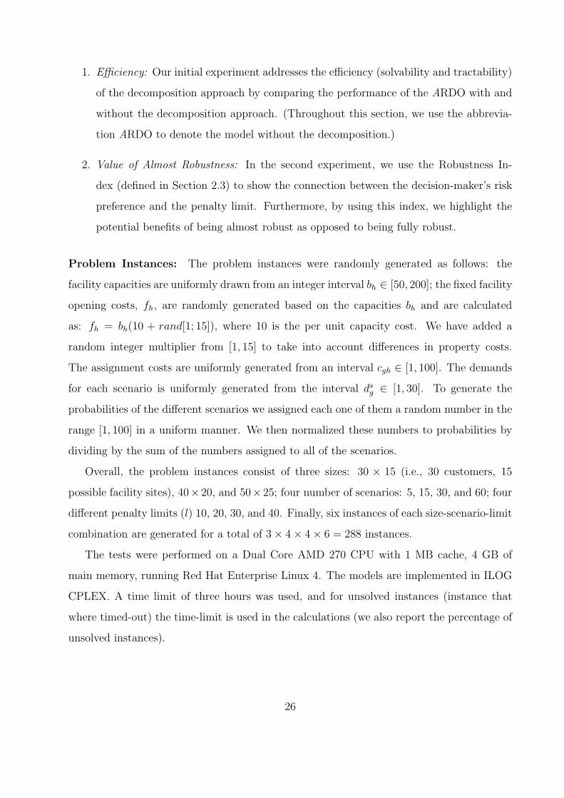
5.1 Efficiency of the Decomposition Approach

Figures 1 and 2 illustrate the effects of the number of scenarios on the run-time performance

of the ARDO and the decomposition approach. As can be seen, the mean and median run

time of the ARDO drastically increases with the number of scenarios. However, the number

of scenarios has only a minor effect if any on the run time of the decomposition approach.

Table 2 gives the mean, median, and the 10th and 90th percentiles of the CPU time in

seconds required to solve each problem instance for each scenario size for the ARDO and

the decomposition approach. The column labeled “% Uns.” indicates the percentage of

the problems for which the models were terminated because of the time limit (of 3 hours).

For the decomposition approach, the column labeled “Iter.” indicates the average number

of iterations needed to converge to optimality. The “Time ratio” for a given instance is

calculated as the ARDO runtime divided by the decomposition run-time. The mean over

each instance in each subset was then calculated.

As Table 2 indicates the decomposition model is very efficient. Specifically, the Decom-

position approach is unable to find the optimal solution within the time limit in only 1.0%

of instances, while the ARDO is unable to find the optimal solution in 19.5% of the in-

stances. For the ARDO, we see an increasing trend in the number of unsolved instance as

27

ARDO DecompositionNumber Time Time Time

of Mean Median Percentile % Uns. Mean Median Percentile % Uns. % Iter. RatioScenarios 10 90 10 90

5 655 13.2 1.13 309.41 4.2 258 2.1 0.24 61.77 1.3 3.2 1815 1188 98.9 4.17 1187.98 6.9 133 4.9 0.28 72.59 0 2.4 9130 3238 557.4 18.39 10800 23.6 248 3.2 0.33 65.63 1.3 3.4 24060 5524 5883.7 70.67 10800 43.1 286 5.1 0.28 77.78 1.3 3.1 566

Overall 2651 222.8 5.03 10800 19.5 231 3.7 0.27 70.73 1.0 3.0 229

Table 2: The mean, median, and the 10th and 90th percentiles of the CPU time (in Seconds) and percentageof unsolved problem instances (“%Uns.”) for the ARDO and decomposition approaches, and the meannumber of iterations (“Iter.”) for the decomposition approach. “Overall” indicates the mean results over allproblem instances.

the number of scenarios increases (up to 43.1%). Furthermore, as the time ratios indicate,

on average, the decomposition approach is 229 times faster than ARDO. We again see an

increasing trend of the time ratios as the number scenarios increase (up to 566). Finally, the

table demonstrates that the decomposition approach converges to optimality on average in

3 iterations.

Figure 3 shows a scatterplot of the run-times for both the ARDO and the decomposition

approach. Both axes are log-scaled, and the points below the x = y line indicate a lower

runtime for the decomposition approach. On all but 8 of the 288 instances (over 97%), the

decomposition achieves equivalent or better run-time (Note that 6 out of the 8 instances

that are dominated are for the problem instances with 5 scenarios).

11,0000.01 0.1 1 10 100 1000

11,000

0.01

0.1

1

10

100

1000

ARDO CPU Time

Decom

posit

ion C

PU

Tim

e

60 Scenarios

30 Scenarios

15 Scenarios

5 Scenarios

Figure 3: Runtime of the ARDO (x Axis, Log-Scale) vs. decomposition model (y Axis, Log-Scale)

28

We summarize this discussion with the following observation:

Observation 1. (Tractability of the decomposition approach) The decomposition

approach is computationally more tractable than the ARDO, i.e., it is up to three orders-

of-magnitude faster, and can find the optimal solution for many more problems within the

time limit.

5.2 Value of Almost Robustness

In this section, by using the Robustness Index in (5), we computationally investigate the

trade-off between the changes in the objective function and in the penalty as the penalty

limit changes. This investigation demonstrates how the Robustness Index can be used by

the decision makers to choose an appropriate penalty limit to better suit her risk preferences.

It also highlights the benefits of being almost robust as opposed to fully robust.

To study the Robustness Index, we calculated it for all the problem instances discussed

earlier for the capacitated facility location problem with uncertain demand. We summarized

the results in Table 3 and Figure 4. In Table 3, we show the mean, median, max, and

the 10th and 90th percentiles of the Robustness Index over all problems instances with a

particular l value. Figure 4 depicts the changes in the average Robustness Index (the average

is taken over all the instances with a given l) as a function the penalty limit. As expected

from the discussion in Section 2.3, as the penalty limit increases the average incremental

improvement in the objective function value increases slower than the average incremental

increases in the penalty. Therefore, it may not be necessary for the decision maker to choose

a very high penalty limit since her relative gain (in terms of improvement in the solution

value) may not grow as fast as the loss (in terms of the penalty).

This experiment also demonstrates that allowing a small amount of infeasibility can

substantially improve the solution value. Specifically, from Table 3 we can see that as we go

from l = 0 to l = 5 the Robustness Index can be as high as 1397, which indicates that the

improvement in the objective function value can be up to 1397 times more than the expected

penalty. This suggests that the solution of the ARO model can be (substantially) less

conservative than that of the robust model, and therefore, highlights the potential benefits

29

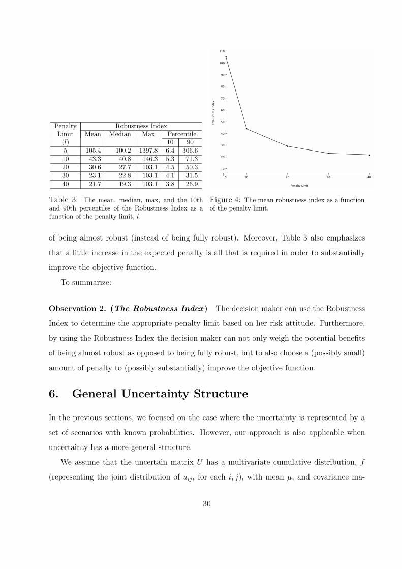
Penalty Robustness IndexLimit Mean Median Max Percentile(l) 10 905 105.4 100.2 1397.8 6.4 306.610 43.3 40.8 146.3 5.3 71.320 30.6 27.7 103.1 4.5 50.330 23.1 22.8 103.1 4.1 31.540 21.7 19.3 103.1 3.8 26.9

Table 3: The mean, median, max, and the 10thand 90th percentiles of the Robustness Index as afunction of the penalty limit, l.

5 10 20 30 40

110

5

10

20

30

40

50

60

70

80

90

100

Penalty Limit

Robustn

ess Index

Figure 4: The mean robustness index as a functionof the penalty limit.

of being almost robust (instead of being fully robust). Moreover, Table 3 also emphasizes

that a little increase in the expected penalty is all that is required in order to substantially

improve the objective function.

To summarize:

Observation 2. (The Robustness Index) The decision maker can use the Robustness

Index to determine the appropriate penalty limit based on her risk attitude. Furthermore,

by using the Robustness Index the decision maker can not only weigh the potential benefits

of being almost robust as opposed to being fully robust, but to also choose a (possibly small)

amount of penalty to (possibly substantially) improve the objective function.

6. General Uncertainty Structure

In the previous sections, we focused on the case where the uncertainty is represented by a

set of scenarios with known probabilities. However, our approach is also applicable when

uncertainty has a more general structure.

We assume that the uncertain matrix U has a multivariate cumulative distribution, f

(representing the joint distribution of uij, for each i, j), with mean µ, and covariance ma-

30

trix Σ, and support Ω(U). Under such uncertainty, based on the available probabilistic

information, the penalty function of constraint j, can take the following forms:

• Expected Penalty Function: Qj(x) = E[(Ujx− bUj )+] =

∫Ω(U)

(Ujx− bUj )+dF, (19),

• Distributionally-Robust Penalty Function: Let F denote the of set of probability dis-

tributions with mean µ and covariance matrix Σ that is assumed to include the true

distribution f . The distributionally-robust penalty function has the form:

Qj(x) = maxf∈FEf [(Ujx− bUj )+], (20).

Therefore, given the appropriate penalty function, the almost robust model with general

uncertainty is:


Qj(x) ≤ lj, j = 1, .., J, (Generalized ARO)x ∈ X.

As an example, when l = 0 (i.e., when no violation is allowed) and Ω(U) is bounded, the

model is equivalent to the robust counterpart, see e.g., Ben-Tal and Nemirovski (1998) and

Ben-Tal et al. (2009), where the uncertain parameter belonged to the uncertainty set Ω(U).

Due to the multidimensional integral, which are computationally prohibitive when the

dimension exceeds four (see Chen and Sim (2009)), the Generalized ARO (even with con-

tinues variables) may be computationally intractable. Therefore, it may be essential to find

tractable approximation for the penalty function. For each constraint j, let vector U j de-

notes the mean of Uj and Σj denotes the corresponding covariance matrix. The next lemma

provides a distribution-free bound denoted by Bj(x) on the penalty function:

Lemma 1. (Distribution free bound on the penalty function)

Ef [(Ujx− bUj )+] ≤ 1

2((U jx− bUj ) +

√ΣjxxT + (U jx− bUj )

2) = Bj(x), ∀f ∈ F. (21).

Proof. It is easy to see:

31

(Ujx− bUj )+ =

|Ujx−bUj |+(Ujx−bUj )

2, (22).

By taking the expectation of both sides of equation (22), and applying the Cauchy-Schwarz

inequality to Ef |Ujx− bUj |, we obtain the bound.

Using the above bound, we can present the following second-order cone programming

approximation of the Generalized ARO model,


Bj(x) ≤ lj, j = 1, .., J, (Approximate ARO)x ∈ X.

It is easy to see that since Qj(x) ≤ Bj(x), the optimal solution of the Approximate ARO

model is a feasible (and conservative) solution of the Generalized ARO model.

Generalized ARO with discrete variables: If the decision variables of the Gener-

alized ARO model are discrete, the model becomes even more intractable. Fortunately,

the decomposition model can be modified to solve such problems. As before, we use

the first moment matrix, U , in the mater problem. Furthermore, the subproblem fol-

lows the same steps as in Section 3: (i)In the penalty calculation step of the subprob-

lem, we calculate Qj(xt) = E[(Ujx

t − bUj )+] (if we have full probabilistic knowledge) or

Qj(xt) = maxfEf [(Ujx

t − bUj )+] (if we have partial probabilistic knowledge). Note that in

circumstances where calculating Qj(xt) is not computationally feasible, we can instead cal-

culate Bj(xt). Doing so however, can result in finding more conservative solutions. (ii) In

the feasibility check step we examine if any penalty constraints is violated. (iii) Finally, in

the cut generation step, the following modified cuts are generated and added to the master

problem:

Qj(xt)− ((U j xtT )(I − x xt)− U j((I − xt) x)) ≤ lj, ∀j ∈ V t. (23)

Corollary 1. (Optimality of the decomposition approach with general uncer-

tainty If the Generalized ARO with discrete variable has an optimal solution, the decompo-

sition approach produces an optimal solution for it in a finite number of iterations.

32

7. Conclusions

In this paper, we presented the Almost Robust Optimization model that is simple, intuitive,

flexible, and easy to communicate to managers. This model allows uncertainty in the deci-

sion making process and bridges stochastic programming and robust optimization. We also

developed a practical and computationally tractable decomposition approach to efficiently

solve the Almost Robust Optimization model with discrete (binary) decision variables. Fur-

thermore, we defined and studied the Robustness Index that can be used by decision makers

to adjust the ARO model to better suit her risk preferences. By using this index we also

demonstrated the potential advantages of being almost robust as opposed to being fully

robust.

We believe that the approach of Almost Robust Optimization is applicable in many

settings and for many problems. We hope that this approach will be used in many future

studies. We also intend to establish additional theoretical results on the solvability of ARO

problems and the Robustness Index for different families of optimization models.

Appendix A - Proofs

Proof. of Theorem1. As explained in Section 3, conditions 1 and 2 are sufficient to establish

Theorem 1. We first prove condition 2, that the cuts (6) are valid. We start by establishing

2(i), i.e., that the cut excludes the current infeasible master problem solution from all sub-

sequent solutions. Suppose the optimal master problem solution is infeasible in iteration t.

Then there exist at least one penalty constraint, i, such that:

Qi(xt) > li. (A1)

Then, the generated cut for this constraint, from (6), is

Qi(xt)−

∑s∈St

i

ps((Usi xtT )(I − x xt)− U s

i ((I − xt) x)) ≤ li. (A2)

If the same solution xt is found in future iterations, (U si xtT )(I−xtxt)−U s

i ((I−xt)xt) = 0,

so that the left hand side of (A2) equal to Qi(xt) that from (A1) is greater than li, creating

a contradiction. Thus, xt is infeasible in future iterations of the master problem.

33

We now prove 2(ii), that is, the proposed cuts do not remove any feasible solution of the

ARDO: let xw be a feasible solution of ARDO found in iteration w > t,

Qj(xw) ≤ lj, j = 1, .., J. (A3)

We define x10 = xt (I − xw), x11 = xt xw, and x01 = (I − xt) xw. Thus, x10 is a vector

with elements equal to 1 if these elements are 1 in xt and 0 in xw, 0 otherwise. Similarly, x11

is a vector with elements equal to 1 if these elements are 1 in both xt and xw, 0 otherwise.

Finally, x01 is a vector with elements equal to 1 if these elements are 0 in xt and 1 in xw, 0

otherwise.

We present a proof by contradiction. Assume that xw does not satisfy a cut formed in

iteration t for constraint i. Since the elements that are 1 in x11 are not included in the cut,

they do not contribute to the LHS of (A2). Thus, from the LHS of (A2) when x = xw,

Qi(xt)−

∑s∈St

i

ps(Usi x

10 − U si x

01) > li. (A4)

Furthermore, since U si x

t = U si x

10 + U si x

11, Qi(xt) can be rewritten as,

Qi(xt) =

∑s∈S

ps(Usi x

10 + U si x

11 − bUi )+ =

∑s∈St

i

ps(Usi x

10 + U si x

11 − bUi ), (A5)

where the last equality follows by only summing over the scenarios with non-negative penal-

ties, Sti . Therefore, by replacing Qi(x

t) in the LHS of (A4) by (A5) we have∑s∈St

i

ps(Usi x

11 + U si x

01 − bUi ) > li. (A6)

Since U si x

w − bUi = U si x

11 +U si x

01− bUi , thus, Qi(xw) =

∑s∈S

ps(Usi x

w − bUi )+ =

∑s∈S

ps(Usi x

11 +

U si x

01 − bUi )+. Therefore,

Qi(xw) =

∑s∈S

ps(Usi x

11 + U si x

01 − bUi )+

=∑s∈St

i

ps(Usi x

11 + U si x

01 − bUi )+ +

∑s∈S−St

i

ps(Usi x

11 + U si x

01 − bUi )+

≥∑s∈St

i

ps(Usi x

11 + U si x

01 − bUi )+

≥∑s∈St

i

ps(Usi x

11 + U si x

01 − bUi )

> li. (A7)

34

where the first inequality is due to∑

s∈S−Sti

ps(Usi x

11 + U si x

01 − bUi )+ ≥ 0, the second due to

(U si x

11 + U si x

01 − bUi ) ≤ max0, (U si x

11 + U si x

01 − bUi ), and the last from (A6). Therefore,

from (A7) we have Qi(xw) > li which contradicts (A3) and thus, our assumption that the

feasible solution xw does not satisfy the cut. This establishes that the cut does not remove

any feasible solution of ARDO.

Since both conditions 2(i) and 2(ii) are satisfied, we conclude that the cut is valid.

We now prove condition 1, that the optimal objective value of the master problem is

a lower bound on that of the ARDO. We first note that because the cuts are valid, they

do not remove any feasible solution of the ARDO at any iterations of the decomposition.

Moreover, since the objective function and the deterministic constraints of the ARDO also

appear in the master problem, we must only take into consideration the penalty constraints

of the ARDO, Qj(x) =∑s

ps(Usj x− bUj )

+ ≤ lj ∀j, and the expected-value constraints of the

master problem, U jx ≤ l′j ≡∑s

ps(Usj x− bUj ) ≤ lj ∀j. In particular, we must show that any

feasible solution of the ARDO is also feasible to the master problem, i.e., if Qj(x) ≤ lj then

U jx ≤ l′j = lj + bUj . Indeed,

U jx− bUj =∑s

ps(Usj x− bUj ) ≤

∑s

ps(Usj x− bUj )

+ = Qj(x), ∀j. (A8)

Thus, we conclude that any feasible solution of ARDO is also feasible for the master problem.

Therefore, the optimal objective value of master problem is a lower bound on that of the

ARDO.

Since both conditions are satisfied, and since the decision variables have a finite domain,

the decomposition model produces an optimal solution to the ARDO in a finite number of

iterations.

Appendix B - Extension of Results to Different Penalty

Functions

As discussed in Section 2, based on the available probabilistic information, the almost robust

model accommodate various penalty functions. The exposition of the paper focuses on the

expected penalty function. In this section, we modify the decomposition approach to capture

both the worst-case and the distributionally-robust penalty functions.

35

Worst-Case Penalty Function: The following modifications in the decomposition ap-

proach are required: (i) in the master problem, replace the expected value matrix U = Es[Us]

by a minimum matrix U′with elements equal to the minimum of the corresponding ele-

ment over all scenarios; (ii) in Step 1 of the subproblem calculate the maximum penalty

(Qj(xt) = max

sQs

j) instead of the expected penalty; (iii) in Step 2 of the subproblem let stj

denote the scenario with the maximum penalty; and (iv) in Step 3 use the modified cut:

Qj(xt)− (U

stjj xtT )(I − x xt)− U

stjj ((I − xt) x) ≤ lj, ∀j ∈ V t. (A16)

Corollary 2. (Convergence of the decomposition approach with the worst-case

penalty function) Cuts of the form (A16) are valid, and the modified decomposition ap-

proach produces an optimal solution to the ARDO with the worst-case penalty function in a

finite number of iterations.

The proof of Theorem 1 directly applies here, we thus omit the proof of Corollary 2.

Distributionally-Robust Penalty Function: Recall that this penalty function is ap-

plicable when the decision maker has limited probabilistic information. Specifically, as is

common in the literature (see Scarf (1958), Bertsimas and Popescu (2005), Yue et al. (2006),

Popescu (2007)), we assume that the decision maker knows that the probability distribution

of the scenarios belongs to a known set of probability distributions, F , and has an estimate

of the first moment of the uncertain matrix, U .

The following modifications in the decomposition approach are required: (i) as in the

decomposition approach use the first moment matrix, U , in the mater problem (if no infor-

mation on first moment is available, use U′, as described for the worst-case penalty function);

(ii) in Step 1 of the subproblem, for each uncertain constraint j = 1, .., J calculate the ex-

pected penalty under distribution f , Qf

j (xt) j = 1, .., J, ∀f ∈ F , determine the distribution

with the maximum expected penalty f tj = argmaxf∈FQ

f

j (xt) and let Qj = Q

f tj

j (xt); (iii) in

Step 3 use the modified cuts:

Qj(xt)−

∑s∈St

j

pf tj

s [(U sj xtT )(I − x xt)− U s

j ((I − xt) x)] ≤ lj, ∀j ∈ V t. (A17)

36

Corollary 3. (Convergence of the decomposition approach with the distributionally-

robust penalty function) Cuts of the form (A17) are valid, and the modified decomposition

approach produces an optimal solution to the ARDO with the distributionally-robust penalty

function in a finite number of iterations.

Proof. The proof of condition 2(i) is similar to that in Theorem 1 and is omitted. Similar to

Theorem 1, we use contradiction to prove condition 2(ii): we assume xw is a feasible solution

of the distributionally-robust model, i.e.,

maxf∈FQf

j (xw) ≤ lj, j ∈ 1, .., J , (A18),

that does not satisfy the cut (A17) of constraint i. Therefore, given Qi(xt) = Q

f ti

i (xt) the

cut when x = xw is

Qf ti

i (xt)−∑s∈St

i

pf ti

s [U si x

10 − U si x

01] > li. (A19)

Since Qf ti

i (xt) =∑s∈St

i

pf ti

s [U si x

10 + U si x

11 − bUi ] (as in Theorem 1 we removed superscript + by

summing over Sti ), (A19) is reduced to∑

s∈Sti

pf ti

s [U si x

11 + U si x

01 − bUi ] > li. (A20)

We now have two possible outcomes:

• fwi = argmaxf∈FQ

f

i (xw) ≡ f t

i , i.e., the distribution in iteration w with the maximum

penalty is the same as that of iteration t. Under this condition, maxf∈FQf

i (xw) =∑

s∈Spfwi

s [U si x

11 + U si x

01 − bUi ]+ =

∑s∈S

pf ti

s [U si x

11 + U si x

01 − bUi ]+. From this and following

the argument in (A7) we get a contradiction, thus under this condition, the cut is valid.

• fwi = f t

i . In this case:

maxf∈FQf

i (xw) =

∑s∈S

pfwi

s [U si x

11 + U si x

01 − bUi ]+ ≥

∑s∈S

pf ti

s [U si x

11 + U si x

01 − bUi ]+. (A21)

37

where the inequality is due to that fwi has the maximum expected penalty in iteration

w. From (A21) and following the argument in (A7) we again get a contradiction, thus,

under this condition, the cut is valid.

From the above two conditions we conclude that the cut is always valid. Furthermore,

Ef [Usj x− bUj ] = U jx− bUj ≤ Ef [U

sj x− bUj ]

+, ∀f ∈ F, j = 1, .., J. (A22)

From (A22) and using the same argument as the proof of condition 1 of Theorem 1, we can

conclude that the master problem solution is a lower bound on that of the distributionally-

robust model.

Appendix C - Absolute Value of Infeasibility Measure

An alternative measure of uncertainty is the absolute value of infeasibility, |U sj x−bUj |, which is

suitable for equality constraints where neither upward nor downward infeasibility is desired.

For such measure, we consider the expected penalty function Qj(x) =∑s∈S

ps|U sj x− bUj |. Note

that the max or the distributionally-robust penalty functions introduced in Section 2 could

also be used if full probabilistic information is not available.

The decomposition approach now requires two major modification. First, in step 1 of

the subproblem, we calculate the absolute infeasibility, Qsj(x

t) = |U sj x

t − bUj |, j = 1, .., J .

Second, in step 3, the cuts are modified to take into account both downward and upward

deviations. In order to introduce the modified cuts, let ns,t = 0 if U sj x− bUj > 0 and ns,t = 1

if U sj x− bUj < 0. The cuts are:

Qj(xt)−

∑s∈St

j

ps(−1)ns,t((U s

j xtT )(I − x xt)− U sj ((I − xt) x)) ≤ lj, ∀j ∈ V t. (A9)

As can be seen, the cuts are identical to the cuts presented in (6) with an addition term

(−1)ns,t. ns,t is defined such that in scenarios with downward deviation (ns,t = 1), removing

an element with a positive (negative) coefficients from xt increases (decreases) the penalty of

the scenario (reflected by U sj ((I −xt) x)), while adding an element with negative (positive)

coefficient decreases (increases) the penalty (enforced through (U sj xtT )(I − x xt)). For

scenarios with upward deviation the effects are reversed.

38

Corollary 4. (Convergence of the decomposition approach with the absolute

value measure) Cuts of the form (A9) are valid, and the modified decomposition approach

produces an optimal solution to the ARDO with the absolute value measure in a finite number

of iterations.

Proof. Since the proof of condition 1 and condition 2(i) (see Section 3) is similar to the proof

presented for Theorem 1, we omit it.

We again use contradiction to prove condition 2(ii), thus assume xw is a feasible solution

of the ARDO with the absolute value measure, i.e.,

Qj(xw) ≤ lj j ∈ 1, .., J, (A10)

and it does not satisfy the cut of constraint i (of the form (A9)). Let x10, x11, and x01 be as

defined in Appendix A. From (A9) when x = xw:

Qi(xt)−

∑s∈St

i

ps(−1)ns,t(U s

i x10 − U s

i x01) > li. (A11)

Furthermore, since U si x

t = U si x

10 + U si x

11 and Qi(xt) =

∑s∈St

i

ps|U si x

t − bUi |, (A11) can be

rewritten as,∑s∈St

i

ps(|U si x

10 + U si x

11 − bUi | − (−1)ns,t(U s

i x10 − U s

i x01)) > li. (A12)

We define Sti+= s ∈ St

i |ns,t = 0 to be the set of scenarios with upward deviation, i.e.,

U si x

t − bUi > 0 ∀s ∈ Sti+, and St

i−

= s ∈ Sti |ns,t = 1 to be the set of scenarios with

downward deviation, i.e., U si x

t − bUi < 0 ∀s ∈ Sti−. Since U s

i xw = U s

i x11 + U s

i x01, thus

Qi(xw) =

∑s∈S

ps|U si x

w − bUi | =∑s∈S

ps|U si x

11 + U si x

01 − bUi |. Therefore,

Qi(xw) =

∑s∈S

ps|U si x

11 + U si x

01 − bUi |

=∑s∈St

i

ps|U si x

11 + U si x

01 − bUi |+∑

s∈S−Sti

ps|U si x

11 + U si x

01 − bUi |

≥∑s∈St

i

ps|U si x

11 + U si x

01 − bUi |

=∑

s∈Sti+

ps|U si x

11 + U si x

01 − bUi |+∑

s∈Sti−ps|U s

i x11 + U s

i x01 − bUi |

≥∑

s∈Sti+

ps(Usi x

11 + U si x

01 − bUi ) +∑

s∈Sti−ps(−(U s

i x11 + U s

i x01 − bUi ))

=∑s∈St

i

ps(|U si x

10 + U si x

11 − bUi | − (−1)ns,t(U s

i x10 − U s

i x01))

39

> li. (A13)

where the first inequality is due to∑

s∈S−Sti

ps|U si x

11 + U si x

01 − bUi | ≥ 0, the second due to

|U si x

11 +U si x

01− bUi | ≥ (−(U si x

11 +U si x

01− bUi )), the last equality is by the definition of ns,t

and Sti+and St

i−, and the last inequality is from (A12).

From (A13) we have Qi(xw) > li, which contradicts (A10). Therefore, the cut does not

remove any feasible solution of ARDO with the absolute value measure (condition 2(ii)).

40

References

Atamturk, A. 2006. Strong formulation of robust mixed 0-1 programming. Mathematical program-ming 108 235–250.

Atamturk, A., M. Zhang. 2007. Two-stage robust netwrok flow and design under uncertainty.Operations Research 55, No. 4 662–673.

Averbakh, I. 2001. On the complexity of a class of combinatorial optimization problems withuncertainty. Mathematical Programming 90 263–272.

Baron, O., J. Milner, H. Naseraldin. 2011. Facility location: A robust optimization approach.Production and Operations Management 20(5) 772–785.

Ben-Tal, A., D. Bertsimas, D. B. Brown. 2010. A soft robust model for optimization under ambi-guity. Operations research 58(4-part-2) 1220–1234.

Ben-Tal, A., S. Boyd, A. Nemirovski. 2006. Extending scope of robust optimization: Comprehensiverobust counterparts of uncertain problems. Mathematical Programming 107(1-2) 63–89.

Ben-Tal, A., L. El Ghaoui, A. Nemirovski. 2009. Robust Optimization. Princeton University Press.

Ben-Tal, A., A. Nemirovski. 1998. Robust convex optimization. Mathematics of operations research23(4) 769–805.

Ben-Tal, A., A. Nemirovski. 1999. Robust solutions to uncertain programs. Operations ResearchLetters 25 1–13.

Ben-Tal, A., A. Nemirovski. 2000. Robust solutions of linear programming problems contaminatedwith uncertain data. Mathematical Programming 88(3) 411–424.

Ben-Tal, A., A. Nemirovski. 2001. Robust optimization-methodology and applications. Mathemat-ical programming 92(3) 453–480.

Benders, J. 1962. Partitioning procedures for solving mixed-variables programming problems. Nu-merische Mathematik 4(1) 238–252.

Bertsimas, D., I. Popescu. 2005. Optimal inequalities in probability theory: A convex optimizationapproach. SIAM Journal on Optimization 15(3) 780–804.

Bertsimas, D., M. Sim. 2003. Robust discerete optimization and network flow. Mathematicalprogramming 98 49–71.

Bertsimas, D., M. Sim. 2004. The price of robustness. Operations Research 52(1) 35–53.

Bertsimas, D., R. Weismantel. 2005. Optimization over integers. Athena Scientific.

Blankenship, J. W., J.E. Falk. 1976. Infinitely constrained optimization problems. Journal ofOptimization Theory and Applications 19(2) 261–281.

Charnes, A., W.W. Cooper. 1959. Chance-constrained programming. Management Science 5 73–79.

Chen, W., M. Sim. 2009. Goal-driven optimization. Operations Research 57(2) 342–357.

Chen, X., M. Sim, P. Sun. 2007. A robust optimization perspective to stochastic programming.Operations Research 55(6) 1058–1071.

El-Ghaoui, L., F. Oustry, H. Lebret. 1998. Robust solutions to uncertain semidefinite programs.SIAM Journal on Optimization 9 33–52.

Fazel-Zarandi, M. M., O. Berman, J.C. Beck. 2012. Solving a stochastic facility/location fleetmanagement problem with logic-based benders de. IIE Transactions, Forthcoming .

Geoffrion, A. M., G. W. Graves. 1974. Multicommodity distribution system design by Bendersdecomposition. Management Science 20(5) 822–844.

41

Hooker, J. N., G. Ottosson. 2003. Logic-based Benders decomposition. Mathematical Programming96 33–60.

Klein Haneveld, W.K. 1986. On integrated chance constraints. Duality in Stochastic Linear andDynamic Programming . Springer, 113–138.

Kouvelis, P., G. Yu. 1997. Robust discerete optimization and its appliastions. Kluwer AcademicPublishKlu, Norwell, MA.

Laporte, G., F. Louveaux. 1993. The integer L-shaped method for stochastic integer programs withcomplete recourse. Operations Research Letters 13 133–142.

Lenstra, J. K., A. H. G. Rinnooy Kan. 1981. Complexity of vehicle routing and scheduling problems.Networks 11(2) 221–227.

Mirchandani, P.B., R.L. Francis. 1990. Discrete Location Theory . Wiley-New York.

Mulvey, J.M., Vanderbei, S.A. R.J., Zenios. 1995. Robust optimization of large-scale systems.Operations Research 43 264–281.

Natarajan, K., D. Pachamanova, M. Sim. 2008. Incorporating asymmetric distributional informa-tion in robust value-at-risk optimization. Management Science 54(3) 573–585.

Natarajan, K., D. Pachamanova, M. Sim. 2009. Constructing risk measures from uncertainty sets.Operations Research 57(5) 1129–1141.

Nemhauser, G.L., L.A. Wolsey. 1988. Integer and combinatorial optimization. Wiley-Interscience,New York, NY, USA.

Papadimitriou, C.H. 2003. Computational complexity. Encyclopedia of Computer Science. JohnWiley and Sons Ltd.

Popescu, I. 2007. Robust mean-covariance solutions for stochastic optimization. Operations Re-search 55(1) 98–112.

Ruszczynski, A., A. Shapiro, eds. 2003. Stochastic Prog . Handbooks in Operations Research andManagement Science, Vol. 10. Elsevier, Amestredam.

Scarf, H. 1958. A min-max solution of an inventory problem. Studies in The Mathematical Theoryof Inventory and Production 2001–2009.

Soyster, A. L. 1973. Convex programming with set-inclusive constraints and applications to inexactlinear programming. Operations Research 21 1154–1157.

Wolsey, L. A. 1998. Integer programming . Wiley-Interscience, New York, NY, USA.

Yue, J., B. Chen, M.-C. Wang. 2006. Expected value of distribution information for the newsvendorproblem. Operations Research 54(5) 1128–1136.

42

almost robust optimization with binary variables robust... · almost robust optimization with...

Documents