all my homeworks - drexel university

All my Homeworks

Prakash Gautam

June 12, 2019

1

PrefaceThis document is the collection of the homework that I did during my time in Drexel University. You canfind the individual homework for each course in my university webpage, which also contains link to somesupporting documents like some python scripts I used and Cadabra2 stuffs I used for my tensor relatedworks. This document is formatted in a book format where each chapter is a course and each section (namedHomework One ... and so on) are the individual homemwork. If a problem is from the coursebook, thenthe problem number starts with the reference to the book and problem number in boldface within a pair ofparenthesis.

As a caution, the solutions have a lot of errors. Honestly, after I got the graded homework back I have notmade any serious attempt to look back my homework and correct them. I would say there is at least anaverage ∼10% overall mistake in the solutions. Apart from the incorrect solutions, there are few noticableerrors and typos. There are some incomplete homework solutions too, which is partly because I did not havethat last extra hour before the due date to typeset.

The way I typeset my homework has evolved considerably over the course of the period I did all these home-works. I took some time to reformat/reorganize the old files but it this has not been complete significantly.Also, there are very obvious errors like some broken references and stuffs. So the problem in correcting thoseerrors is not as trivial as it sounds sometimes. I usually organize my work in a hierarchial directory structure,and in compiling this one as a single monolithic document, I had to make sure that the relative input werecorrect. I got that part by a very clever trick, which I might share in a blog post, if I get in a mood to do so.

Then there is a problem of dublicate reference, which I am sure are plenty in document. This basicallycomes from the fact that when I originally did individual homework, I did not intend to compile them intoa single document, and so the anchor labels were defined to be unique just within that one document, whenI compiled them together there were a few that clashed, which I noticed and tried to correct. After the firsttime I compiled this big document, I started making sure that the individual homework would have thatextra prefix so as to identify it uniquly, but I can’t gurantee that it is error free in that regard too.

I would say most of what I have done here is completely my own work, apart from obvious inspiration Ifound in the internet off of other peoples work. I would say the one I have most influence from internet ismy Electromagnetic theory II homework. One major part of the reason was that I did not put up as muchas work in my coursework as I needed to, especially in the homework (I know what you are thinking at thispoint of time, let me tell you I have watched this video too). But still then most of them is my own workexcept when it is not. Since I did not plagiarize the thing, I have not given credit.

I owe a great deal of thank to my Professors for assigning these homework. Some of the unique homeworkproblem they have desined have got me into serious thinking a lot of the time. Some times when I have beenable to come up with the correct answer to these custom problem, it has given me as much joy as anything.I owe a huge thanks to my class mates, Andrew Antczak1, Sean Lewis, Steve Sclafani, Wexiang2 Yu, withwhom I have had extensive discussion. Some of the works here are our collective work as a whole group oras pair or trio.

I would appreciate any comment or feedback. Any comment or feedback can be directed to [email protected] might update this in the future.

Prakash Gautam,2019 Jun 12

1I am pretty sure I spelt his last name correct2I am positive I spelt this one correct too

http://www.physics.drexel.edu/~pgautam/courses/

https://cadabra.science/

https://www.youtube.com/watch?v=mm-4PltMB2A

mailto:[email protected]

Contents

1 Mathematical Physics 41.1 Homework One . . . . . . . . . . . . . . . . . . . . . . . . . . . . . . . . . . . . . . . . . . . . 41.2 Homework Two . . . . . . . . . . . . . . . . . . . . . . . . . . . . . . . . . . . . . . . . . . . . 111.3 Homework Four . . . . . . . . . . . . . . . . . . . . . . . . . . . . . . . . . . . . . . . . . . . . 201.4 Homework Five . . . . . . . . . . . . . . . . . . . . . . . . . . . . . . . . . . . . . . . . . . . . 261.5 Homework Six . . . . . . . . . . . . . . . . . . . . . . . . . . . . . . . . . . . . . . . . . . . . 33

2 Galactic Astrophysics 422.1 Homework One . . . . . . . . . . . . . . . . . . . . . . . . . . . . . . . . . . . . . . . . . . . . 422.2 Homework Two . . . . . . . . . . . . . . . . . . . . . . . . . . . . . . . . . . . . . . . . . . . . 472.3 Homework Three . . . . . . . . . . . . . . . . . . . . . . . . . . . . . . . . . . . . . . . . . . . 502.4 Homework Four . . . . . . . . . . . . . . . . . . . . . . . . . . . . . . . . . . . . . . . . . . . . 542.5 Homework Five . . . . . . . . . . . . . . . . . . . . . . . . . . . . . . . . . . . . . . . . . . . . 592.6 Homework Six . . . . . . . . . . . . . . . . . . . . . . . . . . . . . . . . . . . . . . . . . . . . 63

3 Quantum Mechanics 673.1 Homework One . . . . . . . . . . . . . . . . . . . . . . . . . . . . . . . . . . . . . . . . . . . . 673.2 Homework Two . . . . . . . . . . . . . . . . . . . . . . . . . . . . . . . . . . . . . . . . . . . . 703.3 Homework Three . . . . . . . . . . . . . . . . . . . . . . . . . . . . . . . . . . . . . . . . . . . 733.4 Homework Four . . . . . . . . . . . . . . . . . . . . . . . . . . . . . . . . . . . . . . . . . . . . 763.5 Homework Five . . . . . . . . . . . . . . . . . . . . . . . . . . . . . . . . . . . . . . . . . . . . 803.6 Homework Six . . . . . . . . . . . . . . . . . . . . . . . . . . . . . . . . . . . . . . . . . . . . 843.7 Homework Seven . . . . . . . . . . . . . . . . . . . . . . . . . . . . . . . . . . . . . . . . . . . 863.8 Homework Eight . . . . . . . . . . . . . . . . . . . . . . . . . . . . . . . . . . . . . . . . . . . 91

4 Mathematical Physics II 954.1 Homework One . . . . . . . . . . . . . . . . . . . . . . . . . . . . . . . . . . . . . . . . . . . . 954.2 Homework Two . . . . . . . . . . . . . . . . . . . . . . . . . . . . . . . . . . . . . . . . . . . . 984.3 Homework Three . . . . . . . . . . . . . . . . . . . . . . . . . . . . . . . . . . . . . . . . . . . 1004.4 Homework Four . . . . . . . . . . . . . . . . . . . . . . . . . . . . . . . . . . . . . . . . . . . . 1064.5 Homework Five . . . . . . . . . . . . . . . . . . . . . . . . . . . . . . . . . . . . . . . . . . . . 1104.6 Homework Six . . . . . . . . . . . . . . . . . . . . . . . . . . . . . . . . . . . . . . . . . . . . 1164.7 Homework Seven . . . . . . . . . . . . . . . . . . . . . . . . . . . . . . . . . . . . . . . . . . . 1194.8 Homework Eight . . . . . . . . . . . . . . . . . . . . . . . . . . . . . . . . . . . . . . . . . . . 123

5 The Standard Model 1305.1 Homework One . . . . . . . . . . . . . . . . . . . . . . . . . . . . . . . . . . . . . . . . . . . . 1305.2 Homework Two . . . . . . . . . . . . . . . . . . . . . . . . . . . . . . . . . . . . . . . . . . . . 1335.3 Homework Three . . . . . . . . . . . . . . . . . . . . . . . . . . . . . . . . . . . . . . . . . . . 1365.4 Homework Four . . . . . . . . . . . . . . . . . . . . . . . . . . . . . . . . . . . . . . . . . . . . 1415.5 Homework Five . . . . . . . . . . . . . . . . . . . . . . . . . . . . . . . . . . . . . . . . . . . . 1445.6 Homework Six . . . . . . . . . . . . . . . . . . . . . . . . . . . . . . . . . . . . . . . . . . . . 148

2

CONTENTS 3

6 Statistical Mechanics 1526.1 Homework One . . . . . . . . . . . . . . . . . . . . . . . . . . . . . . . . . . . . . . . . . . . . 1526.2 Homework Two . . . . . . . . . . . . . . . . . . . . . . . . . . . . . . . . . . . . . . . . . . . . 1576.3 Homework Three . . . . . . . . . . . . . . . . . . . . . . . . . . . . . . . . . . . . . . . . . . . 1606.4 Homework Four . . . . . . . . . . . . . . . . . . . . . . . . . . . . . . . . . . . . . . . . . . . . 1636.5 Homework Five . . . . . . . . . . . . . . . . . . . . . . . . . . . . . . . . . . . . . . . . . . . . 168

7 Quantum Mechanics II 1757.1 Homework One . . . . . . . . . . . . . . . . . . . . . . . . . . . . . . . . . . . . . . . . . . . . 1757.2 Homework Two . . . . . . . . . . . . . . . . . . . . . . . . . . . . . . . . . . . . . . . . . . . . 1807.3 Homework Three . . . . . . . . . . . . . . . . . . . . . . . . . . . . . . . . . . . . . . . . . . . 1837.4 Homework Four . . . . . . . . . . . . . . . . . . . . . . . . . . . . . . . . . . . . . . . . . . . . 185

8 Statistical Mechanics II 1888.1 Homework One . . . . . . . . . . . . . . . . . . . . . . . . . . . . . . . . . . . . . . . . . . . . 1888.2 Homework Two . . . . . . . . . . . . . . . . . . . . . . . . . . . . . . . . . . . . . . . . . . . . 1928.3 Homework Three . . . . . . . . . . . . . . . . . . . . . . . . . . . . . . . . . . . . . . . . . . . 1968.4 Homework Four . . . . . . . . . . . . . . . . . . . . . . . . . . . . . . . . . . . . . . . . . . . . 200

9 Particle Physics 2059.1 Homework One . . . . . . . . . . . . . . . . . . . . . . . . . . . . . . . . . . . . . . . . . . . . 2059.2 Homework Two . . . . . . . . . . . . . . . . . . . . . . . . . . . . . . . . . . . . . . . . . . . . 2099.3 Homework Three . . . . . . . . . . . . . . . . . . . . . . . . . . . . . . . . . . . . . . . . . . . 2099.4 Homework Four . . . . . . . . . . . . . . . . . . . . . . . . . . . . . . . . . . . . . . . . . . . . 212

10 Classical Electrodynamics 21710.1 Homework One . . . . . . . . . . . . . . . . . . . . . . . . . . . . . . . . . . . . . . . . . . . . 21710.2 Homework Two . . . . . . . . . . . . . . . . . . . . . . . . . . . . . . . . . . . . . . . . . . . . 21910.3 Homework Three . . . . . . . . . . . . . . . . . . . . . . . . . . . . . . . . . . . . . . . . . . . 22310.4 Homework Four . . . . . . . . . . . . . . . . . . . . . . . . . . . . . . . . . . . . . . . . . . . . 22810.5 Homework Five . . . . . . . . . . . . . . . . . . . . . . . . . . . . . . . . . . . . . . . . . . . . 23110.6 Homework Six . . . . . . . . . . . . . . . . . . . . . . . . . . . . . . . . . . . . . . . . . . . . 238

11 Classical Electrodynamics II 24011.1 Homework One . . . . . . . . . . . . . . . . . . . . . . . . . . . . . . . . . . . . . . . . . . . . 24011.2 Homework Two . . . . . . . . . . . . . . . . . . . . . . . . . . . . . . . . . . . . . . . . . . . . 24511.3 Homework Three . . . . . . . . . . . . . . . . . . . . . . . . . . . . . . . . . . . . . . . . . . . 24911.4 Homework Four . . . . . . . . . . . . . . . . . . . . . . . . . . . . . . . . . . . . . . . . . . . . 25511.5 Homework Five . . . . . . . . . . . . . . . . . . . . . . . . . . . . . . . . . . . . . . . . . . . . 258

12 General Relativity 26012.1 Homework One . . . . . . . . . . . . . . . . . . . . . . . . . . . . . . . . . . . . . . . . . . . . 26012.2 Homework Two . . . . . . . . . . . . . . . . . . . . . . . . . . . . . . . . . . . . . . . . . . . . 26212.3 Homework Three . . . . . . . . . . . . . . . . . . . . . . . . . . . . . . . . . . . . . . . . . . . 26812.4 Homework Four . . . . . . . . . . . . . . . . . . . . . . . . . . . . . . . . . . . . . . . . . . . . 26912.5 Homework Five . . . . . . . . . . . . . . . . . . . . . . . . . . . . . . . . . . . . . . . . . . . . 27712.6 Homework Six . . . . . . . . . . . . . . . . . . . . . . . . . . . . . . . . . . . . . . . . . . . . 286

Chapter 1

Mathematical Physics

1.1 Homework One1.1.1. Let a and b be any two vectors in a real linear vector space, and define c = a+ λb , where is real. By

requiring that c ≥ 0 for all λ, derive the Cauchy-Schwartz inequality

(a · a)(b · b) ≥ (a, b)2

When does equality hold? (Use only the general properties of the inner product. Do not assume thatit is possible to write a.b = |a||b| cos(θ)Solution:Lets assume c = a+ λb, then by the definition of inner product we get (c.c) ≥ 0

c.c = (a+ λb)(a+ λb) ≥ 0

⇒ ((a+ λb).a) + λ(a+ λb).b) ≥ 0 Linearity of inner product⇒ (a.a) + λ(b.a) + λ(a.b) + λ2(b.b) ≥ 0 Linearity of inner product with λreal⇒ (a.a) + 2λ(a.b) + λ2(b.b) ≥ 0 (a.b) = (b.a) for real vector space

The above inequality is quadratic in λ which is real value. All the inner product map to real valuesin this real linear space. The equality of above expression is a quadratic equation of in r with realcoefficient. Since the quadriatic equation lies wholely above real axis it can’t have real solution. Thecondition for which is

4(a.a)(b.b) ≤ (2(a.b))2

(a.a)(b.b) ≤ (a.b)2.

Clearly the equality hold when the two vectors are identical.

1.1.2. Let A be any square matrix, and define B = eA ≡∞∑

n=0

An

n!Prove that an eivenvector of A with

eigenvalue λ is an eigenvector of B, with eigenvalue eλ.Solution:Given λ is eigenvalue of A. Let the corresponding eivenvector be C. By defition

AC = λC

Pre multiplying above relation with A we get.

4

CHAPTER 1. MATHEMATICAL PHYSICS 5

A(AC) = A(λC)⇒ (AA)C = λ(AC)⇒ A2C = λλC = λ2C

By induction we getAnC = λnC (1.1)

Now lets operate the vector C by B

BC =

( ∞∑n=0

An

n!

)C (Definition of B Given)

=

∞∑n=0

1

n!AnC (Distributive property of Matrix over Matrix)

=

∞∑n=0

1

n!λnC (From (1.1))

=

( ∞∑n=0

λn

n!

)C (Distributive property of scalar over matrix)

= eλC (Definition of e)

Since BC = eλC, C is the eigenvector of B with eigenvalue eλ.

1.1.3. Consider the 4-dimensional vector space of polynomials of degree less than or equal to 3, on the range1 ≤ x ≤ 1, spanned by the basis set

1, x, x2, x3

.The inner product of two polynomials in this space

is defined as(f, g) =

∫ 1

−1

|x|f(x)g(x)dx

Use Gram–Schmidt orthogonalization to construct two orthonormal basis sets, as follows:

(a) Start with the set as listed above and begin the procedure with the function 1, as in class.

(b) Rewrite the set as x2, x, 1, x3and begin the orthogonalization procedure starting with x2

Write down the matrix representing the transformation from basis (i) to basis (ii), and demon- stratethat it is orthogonal.Solution:


Let us write the cross product table for the given basis functions.

(1 · 1) =∫ 1

−1

|x|1 · 1dx =

∫ 0

−1

−xdx+

∫ 1

0

xdx =−x2

2

]0−1

+−x2

2

]10

=1

2+

1

2= 1

(1 · x) =∫ 1

−1

|x|1 · xdx =

∫ 0

−1

−x2dx+

∫ 1

0

x2dx =−x3

3

]0−1

+x3

3

]10

= −1

3+

1

3= 0

(1 · x2) =∫ 1

−1

|x|1 · x2dx =

∫ 0

−1

−x3dx+

∫ 1

0

x3dx =−x4

4

]0−1

+x4

4

]10

=1

4+

1

4=

1

2

(1 · x3) =∫ 1

−1

|x|1 · x3dx =

∫ 0

−1

−x4dx+

∫ 1

0

x4dx =−x5

5

]0−1

+x5

5

]10

= −1

5+

1

5= 0

(x · 1) = (1 · x) = 0

(x · x) =∫ 1

−1

|x|x · xdx =

∫ 1

−1

|x|1 · x2dx =1

2

(x · x2) =∫ 1

−1

|x|x · x2dx =

∫ 1

−1

|x|1 · x3dx = 0

(x · x3) =∫ 1

−1

|x|x · x3dx =

∫ 0

−1

−x5dx+

∫ 1

0

x5dx =−x6

6

]0−1

+x6

6

]10

=1

6+

1

6=

1

3

(x2 · 1) = (1 · x2) = 1

2(x2 · x) = (x · x2) = 0

(x2 · x2) =∫ 1

−1

|x|x2 · x2dx =

∫ 1

−1

|x|x · x3dx =1

3

(x2 · x3) =∫ 1

−1

|x|x2 · x3dx =

∫ 0

−1

−x6dx+

∫ 1

0

x6dx =−x7

7

]0−1

+x7

7

]10

= −1

7+

1

7= 0

(x3 · 1) = (1 · x3) = 0 (x3 · x) = (x · x3) = 1

2(x3 · x2) = (x3 · x2) = 0

(x3 · x3) =∫ 1

−1

|x|x3 · x3dx =

∫ 0

−1

−x7dx+

∫ 1

0

x7dx =−x8

8

]0−1

+x8

8

]10

=1

8+

1

8=

1

4

For the first basis set: 1, x, x2, x3; Let (v1, v2, v3, v4) = (1, x, x2, x3) and let (e1, e4, e3, e4) be the corre-sponding orthonormal set.

e1 = v1 = 1 e1 =e1√

(e1, e1)=

1√(1 · 1)

= 1

e2 = v2 − (e1, v2)e1 e2 =x√(x, x)

=1√1/2

=√2x

= x− (1, x)1 = x− 0 = x

The normal vector corresponding to v3 can be found as.


e3 = v3 − (e2, v3)e2 − (e1, v3)e1

= x2 − (√2x, x2)

√2x− (1, x2)1

= x2 −√2(x, x2)

√2x− 1

2

= x2 −√2 · 0 ·

√2x− 1

2

= x2 − 1

2

e3 =x2 − 1/2√

(x2 − 1/2, x2 − 1/2)

=x2 − 1/2√

(x2, x2)− 2(x2, 1/2) + (1/2, 1/2)

=x2 − 1/2√

13 − 2 · 12 ·

12 + 1

4

=√3(2x2 − 1

)For v4 = x2 we similarly get:

e4 = v4 − (e3, v4)e3 − (e2, v4)e2 − (e1, v4)e1

= x3 − (√3(2x2 − 1

), x3)√3(2x2 − 1

)− (√2x, x3)

√2x− (1, x3)1

= x3 −√3(2(x2, x3)− (1, x3)

)√3(2x2 − 1

)−√2(x, x3)

√2x

= x3 −√3 (0− 0)

√3(2x2 − 1

)−√21

3

√2x

= x3 − 0− 2

3x

= x3 − 2

3x

e3 =x3 − (2/3)x√(x3 − 2

3x, x3 − 2

3x)

=x3 − (2/3)x√(

(x3, x3)− 2 23 (x

3, x)− 23

2(x, x)

)=

x3 − (2/3)x√14 − 2 · 23 · 0 +

29

= 6

(x3 − 2

3x

)= 6x3 − 4x

Therefore the orthonormalized basis set is1,√2x,

√3(2x2 − 1), 6x3 − 4x

Working out similarly,

Let (e1′, e4

′, e3′, e4

′) be the corresponding orthonormal set.

e′1 = v1 = x2 e1′ =

e′1√(e′1, e

′1)

=x2√

(x2, x2)=

x2√1/3

=√3x2

e′2 = v2 − (e1′, v2) e2

′ =e′2√

(e′2, e′2)

=x√(x, x)

=1√1/2

=√2x

= x− (√3x2, x)

√3x2

= x−√3 · 0 ·

√3x2 = x

e′3 = v3 − (e2′, v3)e2

′ − (e1′, v3)e1

′

= 1− (√2x, 1)

√2x− (

√3x2, 1)

√3x2

= 1−√2(x, 1)

√2x−

√3(x2, 1)

√3x2

= 1−√2 · 0 ·

√2x−

√3 · 1

2·√3x2

= 1− 3

2x2

(e′3, e′3) =

(1− 3/2x

2, 1− 3/2x2)

= (1, 1)− 2(1,−3/2x2) + (−3/2x

2,−3/2x2)

= 1 + 23/2(1, x2) + (3/2)

2(x2, x2)

= 1 + 2 · 3/2 ·1/2 + (3/2)

20 = 4

e3′ =

e′3√(e′3, e

′3)

=1− 3/2x

2

√4

= 2− 3x2


e′4 = v4 − (e3′, v4)e3

′ − (e2′, v4)e2

′ − (e1′, v4)e1

′

= x3 − (2− 3x2, x3)(2− 3x2)− (√2x, x3)

√2x− (

√3x2, x3)

√3x2

= x3 − (2(1, x3)− 3(x2, x3))(2− 3x2))−√2(x, x3)

√2x−

√3(x2, x3)

√3x2

= x3 − (2 · 0− 3 · 0)(2− 3x2))−√2(1/3)

√2x−

√3(0)√3x2

= x3 −√2(1/3)

√2x = x3 − 2

3x

(e′4, e′4) =

(x3 − 2/3x, x

3 − 2/3x)

= (x3, x3)− 22/3(x3, x) + (2/3)

2(x, x)

= 1/4 − 2 · 2/3 · 0 +2/9

= 1/36

e4′ =

e4√(e4, e4)

=x3 − 2/3x√

1/36= 6x3 − 4x

So the orthonormal basis set is found to be.√3x2,

√2x, −3x2 + 2, 6x3 − 4x

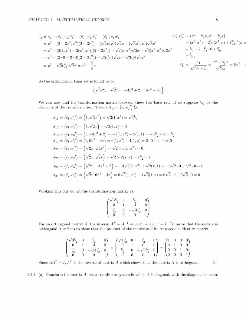
We can now find the transformation matrix between these two basis set. If we suppose λij be theelements of the transformation. Then e λij =

(ei, ej

′) So,

λ11 =(e1, e1

′) = (1,√3x2) =√3(1, x2) =

√31/2

λ12 =(e1, e2

′) = (1,√2x) =√2(1, x) = 0

λ13 =(e1, e3

′) = (1,−3x2 + 2)= −3(1, x2) + 2(1, 1) = −31/2 + 2 = 1/2

λ14 =(e1, e4

′) = (1, 6x3 − 4x)= 6(1, x3) + 4(1, x) = 6 · 0 + 4 · 0 = 0

λ21 =(e2, e1

′) = (√2x,√3x2) =√2× 3(x, x2) = 0

λ22 =(e2, e2

′) = (√2x,√2x) =√2× 2(x, x) = 21/2 = 1

λ23 =(e2, e3

′) = (√2x,−3x2 + 2)= −3

√2(x, x2) +

√2(x, 1) = −3

√2 · 0 +

√2 · 0 = 0

λ24 =(e2, e4

′) = (√2x, 6x3 − 4x)= 6√2(1, x3) + 4

√2(1, x) = 6

√2 · 0 + 2

√2 · 0 = 0

Wroking this out we get the transformation matrix as.√31/2 0 1/2 00 1 0 01/2 0 −

√31/2 0

0 0 0 1

For an orthogonal matrix A, the inverse AT = A−1 ⇒ AAT = AA−1 = I. To prove that the matrix isorthogonal it suffices to show that the product of the matrix and its transpose is identity matrix.

√31/2 0 1/2 00 1 0 01/2 0 −

√31/2 0

0 0 0 1

×√31/2 0 1/2 00 1 0 01/2 0 −

√31/2 0

0 0 0 1

=

1 0 0 00 1 0 00 0 1 00 0 0 1

Since AAT = I, AT is the inverse of matrix A which shows that the matrix A is orthogonal.

1.1.4. (a) Transform the matrix A into a coordinate system in which A is diagonal, with the diagonal elements


increasing from top to bottom. Write down the transformation matrix and the diagonalized A

A =

0 −i 0 0 0i 0 0 0 00 0 2 0 00 0 0 1 −i0 0 0 i 1

(b) A matrix B has real eigenvalues. Does it necessarily follow that B is hermitian? Prove the statementor give a counterexample.Solution:Lets find the eigenvalues of the matrix A. The determinant of (A− λI) is∣∣∣∣∣∣∣∣∣∣

−λ −i 0 0 0i −λ 0 0 00 0 2− λ 0 00 0 0 1− λ −i0 0 0 i 1− λ

∣∣∣∣∣∣∣∣∣∣= λ(λ− 2)2(λ− 1)(λ+ 1) = 0

The solution to the above equation will give λ = −1, 0, 1, 2, 2 The normalized eigenvector correspond-ing to each eigenvalues are.

−1→ 1/√2

i1000

0→ 1/√2

000i1

1→ 1/√2

−i1000

2→ 1/√2

00√200

2→ 1/√2

000−i1

So the transformation matrix to transform A to a diagonal matrix is

P = 1/√2

i 0 −i 0 01 0 1 0 00 0 0 1 00 i 0 0 −i0 1 0 0 1

and its inverse is P−1 = 1/√2

−i 1 0 0 00 0 0 −i 1i 1 0 0 00 0 2 0 00 0 0 i 1

The diagonalization of A is done with P−1AP which is a diagonal matrix.

All matrices with real eigenvalues may not be hermition. Lets for example consider:(1 10 1

). Its

eigenvalue is 1 with multiplicity 2, which is real but the matrix is not Hermitian as:(1 10 1

)†

=

(1 01 1

)=(1 10 1

)

1.1.5. Find the normal modes and normal frequencies for linear vibrations (i.e. vibrations in the horizontaldirection, as drawn) of the (over)simplified “CO2molecule” modeled by the collection of masses andsprings sketched below.Solution:If we suppose the displacement of each mass from their equilibrium position to be x1, x2 and x3, thenthe kinetic energy of the system is the sum of kinetic energy of each masses which is:

T = 1/2Mx12 + 1/2mx2

2 + 1/2Mx32

And the potential energy of the system would be:

V = 1/2k1(x2 − x1)2 + 1/2k1(x3 − x2)

2 + 1/2k2(x3 − x1)


Now using the Lagranges equation of motion:

d

dt

(∂(T − V )

∂xi

)=∂(T − V )

∂xi

Since T is free of xis and V is free of xi we can write the above expression as:

d

dt

(∂T

∂xi

)= − ∂V

∂xi

calculating the above terms we get.

Mx1 = −[(k1 + k2)x1 − k1x2 − k2x3]mx2 = −[ −k1x1 + 2k1x2 − k1x3]Mx3 = −[ −k2x1 − k1x2 + (k1 + k2)x3]

The above set of relation can be written in matrix form as.M 0 00 m 00 0 M

x1x2x3

= −

k1 + k2 −k1 −k2−k1 2k1 −k1−k2 −k1 k1 + k2

x1x2x3

If we suppose that the motion is perfectly harmonic with frequency ω and suppose xk = αe−iωxk Thenxi = −ω2xi. Using these values in above relation we get.

−ω2

M 0 00 m 00 0 M

x1x2x3

= −

k1 + k2 −k1 −k2−k1 2k1 −k1−k2 −k1 k1 + k2

x1x2x3

Writing above equation with matrix form as (B − ω2A)x = 0, we can say that this equation has nontrivial solutions for |B − ω2A| = 0∣∣∣∣∣∣

−Mω2 + k1 + k2 −k1 −k2−k1 2k1 −mω2 −k1−k2 −k1 −Mω2 + k1 + k2

∣∣∣∣∣∣ = 0

⇒ −2k21k2 − 2k21(−Mω2 + k1 + k2

)− k22

(2k1 −mω2

)+(2k1 −mω2

) (−Mω2 + k1 + k2

)2= 0

The solution for ω2 for this equation are:0,

1

M(k1 + 2k2) ,

1

Mm(2Mk1 + k1m)


The first normal mode with ω2 = 0 implies that the system perform oscillation such that the relativeposition of the masses do not change meaning each mass oscillates in same direction with same frequency.

The second normal mode ω2 = 1/M (k1 + 2k2) doesn’t depend upon the mass in the middle. So themiddle mass remains at rest and the two mass at in the end perform oscillation with same frequencybut opposite phase.

The third normal mode ω2 = 1/Mm (2Mk1 + k1m) doesn’t depend on the second spring with springconstant k2 meaning the middle mass oscillates and the mass in the either remain at rest.

1.2 Homework Two1.2.1. An electrical network consists of N interconnected nodes. Each pair of nodes (i, j) is connected by a

resistor of resistance Rij = min(i, j) + 2 max(i, j), for i, j = 1, ..., N . Let Vi be the electrical potentialof node i, and choose the zero level of potential to set V1 = 0. Then Kirchhoff’s laws for the othernodes in the network can be conveniently written as

N∑j=1

Vj − ViRij

= Ii

, for i = 2, ..., N where Ii is the current flowing from node i to some external circuit. Suppose N = 100and the external connection is such that current flows out of node 2 and back into node 1, so I1 = 1,I2 = 1, and Ii = 0 for i > 2. By solving the above (N1)-dimensional matrix equation, calculate thetotal resistance between nodes 1 and 2.Solution:Expanding the ith current value

I1 =V2 − V1R12

+V3 − V1R13

+ · · ·+ VN − V1R1N

= −(

1

R12+

1

R12+ · · ·+ 1

R1N

)V1 +

V2R12

+V3R13

+ · · ·+ VNR1N

Smililarly expanding all others we get the pattern. So the equivalent matrix would be.I1I2I3...IN

=

−(

1R12

+ 1R12

+ · · ·+ 1R1N

)1

R12

1R13

· · · 1R1N

1R21

−(

1R21

+ 1R23

+ · · ·+ 1R2N

)1

R23· · · 1

R2N

... · · ·. . . ...

1RN1

1RN2

1RN3

· · · −(

1RN1

+ 1RN2

+ · · ·+ 1RNN

)

V1V2V3...VN

This is the Matrix equation relating the Ohm’s law where I = VR . The 1/R Matrix is N ×N matrix.

But since V1 is zero and I1 is known we can eleminate the first row and column of 1/R Matrix to get(N − 1) Dimensional Matrix


import numpy as npfrom numpy import linalg as LA

num_nodes = 100#Construct the matrixN = num_nodesdef Res(i,j):

return min(i,j) + 2*max(i,j)

# Construct the R matrix with every elements except the diagonals# int(i!=j) returns 1 for non diagonal places and 0 for diagonal# places so all the diagonal elementsR=np.array([(int(i!=j)*(1/Res(i,j))) for i in range(1,N+1) for j in range(1,N+1)]).reshape(N,

N)

# Since in the matrix we see that the diagonal# elements are simply negative sum of all other# elements in the matrix, we sum them to get the# diagonal elements and put them back to matrixDiag = [-sum(R[i]) for i in range(N)]np.fill_diagonal(R,Diag)

#Deleting the first row and columsR = R[1:,1:]

#Initializing the Current column matrix to zeroI = np.zeros(N-1).reshape(N-1,1)

# The first value of current I_2 is indexed at zero# so I[0] means the I_2 which is 1I[0] = 1

# Solving the matrix equation to get the potentials at all nodesV =LA.solve(R,I).reshape(N-1)

# Since our zero index in program is index 2 for current and voltages# the voltage at node 2 is V[0]V2 = V[0]print('The electric potential at node 2 is :.4V'.format(V[0]))

# The current in the whole circuit is 1A so the equivalent resistance# can be calculated by Ohm's law. R_eq = (V1 - V2) / I, since V1 = 0# The total resistance of circuit is just R_eq = -V2/1 = -V2print('The equivalent Resistance of circuit is Ω:.4'.format(-V[0]))

The electric potential at node 2 is -0.9442VThe equivalent Resistance of circuit is 0.9442Ω

1.2.2. The data file hw2.2.dat on the course Web page contains (hypothetical) experimental data on the mea-surement of a function y(x). The N data points are arranged, one measurement per line, in the format

xi yi (measured) σi

where σi is an estimate of the uncertainty in the i-th measurement. It is desired to find the least-squarefit to the data by polynomials of the form

y(x) =

N∑j=1

ajxj−1

for specified values of m, by minimizing the quantity


χ2 =

N∑i=1

[yi −

∑mj=1 ajx

j−1

σi

]2As discussed in class (and in Numerical Recipes, pp 671–676), write down the overdetermined designmatrix equation that results from writing y(xi) = yi,

Aa = b

, where Aij =xj1i

σi, bi = yi

σi(so the measurement undertainties are included in each row), and a is

the vector of unknown coefficients. Solve this system using singular value decomposition (svdcmp inNumerical Recipes, svd in Python or Matlab) to obtain the best fitting polynomial for each of the casesm = 2, 4, 7, and 13. For each m, give the values of aj and χ2, and plot the data and the best fit on asingle graph.Solution:

#!/usr/bin/env python3

import numpy as npimport numpy.linalg as LAimport matplotlib.pyplot as pltfrom matplotlib2tikz import save as tikz_save

class LeastSquare():mlist = [2,4,7,13]#6,7,8,9,13]pltcnt = len(mlist)pltprm = 221clr = 0.1 #clearence

datafile = './data/hw2.2.dat'slc = 500 # slice length to test for fewer data pointsepsilon = 1e-3 # zero threshold for svd inverting

def __init__(self):self.readfile()

def readfile(self):read = np.genfromtxt(self.datafile)self.x = read[:,0]; self.x = self.x[:self.slc]self.y = read[:,1]; self.y = self.y[:self.slc]self.sd = read[:,2]; self.sd = self.sd[:self.slc]self.err = self.sd.reshape(self.slc,1)return read

def construct_A(self,M):#Reform x shape to column shapexcol = self.x.reshape(self.slc,1)# Same for error valueserr = self.sd.reshape(self.slc,1)

# initialize the first column of the A matrixA = (np.zeros(self.slc) + 1).reshape(self.slc,1)/errfor m in range(1,M):

A = np.append(A,xcol**m/err,1)

return np.matrix(A)

def construct_b(self):coly = self.y.reshape(len(self.y),1)return np.matrix(coly/self.err)

def get_svd_inverse(self,M):


U,W,V = LA.svd(M)WI_star = []for wi in W:

if wi < self.epsilon:WI_star.append(0)

else:WI_star.append(1/wi)

WI = np.diag(WI_star)r,c = M.shapeinc_prm = r-ccm = np.matrix(np.zeros(inc_prm*c).reshape(c,inc_prm))WI = np.hstack([WI,cm])return V.T*WI*U.T

def get_polynomial_values(self,aj,x):y = np.zeros(len(x))for j in range(len(aj)):

y += aj[j]*x**j #since our index starts at 0, it worksreturn y

def get_coefficient(self,m):A = self.construct_A(m)b = self.construct_b()AI = self.get_svd_inverse(A)a = AI*b#print('a shape is '.format(a.shape))ar = np.squeeze(np.asarray(a))return ar

def get_chi_sq(self,true,predicted,error):return np.sum(((true-predicted)/error)**2)

def get_legend(self,aj):j = 2lg = r':.2 + :.2$x$'.format(aj[0],aj[1])for a in aj[j:]:

sgn = ' + 'if a < 0: sgn = ''t = sgn + r':.4$x^'.format(a)+''+''.format(j)+'$'lg += tj += 1

return lg

def draw_graph(self):cnt = 0for m in self.mlist:

#plt.subplot(self.pltprm+cnt); cnt+=1

aj = self.get_coefficient(m)#print('ar was ',ar)x = np.linspace(1.1*min(self.x),1.1*max(self.x),500)y = self.get_polynomial_values(aj,x)

prediction = self.get_polynomial_values(aj,self.x)

chisq = self.get_chi_sq(self.y,prediction,self.err)

plt.plot(x,y,'r',linewidth='2.5',label=self.get_legend(aj))plt.legend()plt.plot(self.x,self.y,'go')plt.title('For M = $\chi^2$=:.3e'.format(m,chisq))plt.savefig('M.png'.format(m))plt.show()

plt.suptitle('M degree polynomial least square fit by SVD')


#tikz_save('Least square plots.tex',figurewidth="14cm",figureheight="9cm")plt.show()

if __name__ == '__main__':LS = LeastSquare()LS.draw_graph()

The aj values are shown as polynomial coefficient in the legend of each plot and the χ2 values are givenat the top of each graph. In each case the continuous line is the fitted polynomial and the scattereddots are the values read from file.

1.2.3.Solution:This Question was mostly solved by use of Sympy package in python.

import numpy as npimport numpy.linalg as LA


from scipy.integrate import quad

import sympy as smpimport sympy.functions as smfimport sympy.physics.quantum.constants as qc

The function ϕn(x) was defined to get any order functiondef fai(self,n):

x = self.x; b = self.bof = smp.Rational(1,4)oh = smp.Rational(1,2)A = (b**2/smp.pi)**of*1/(smp.sqrt(2**n*smf.factorial(n)))return (smp.exp(-oh*b**2*x**2)*smf.hermite(n,b*x)) * A

So for example this function gives for fai(n) as.

2−p2

√|β|

4√π√p!

e−β2x2

2 Hp (βx)


Then the hamiltonial operator function is defined as.

def H(self,psi):hf = smp.Rational(1,2)x = self.x; m = self.m; hcut = self.hcuthctm = -hf*(hcut**2)/(m)return hctm * smp.diff(psi,x,2) + self.V(x)*psi

Writing Ap =2−

p2√

|β|4√π√p!

and after operating ϕp(x) by Hamiltonian operator and using the recurrencerelation we get.

Hϕp(x) =Ape

− β2x2

2

2m

(−β2ℏ2

(β2x2Hp (βx)− 4βpxHp−1 (βx) + 4p (p− 1)Hp−2 (βx)−Hp (βx)

)+ kmx2Hp (βx)

)If we evaluate the functions operated by at numeric value 0.

Hϕ0(x) =Ape

− β2x2

2

2m

(−β2ℏ2

(β2x2 − 1

)+ kmx2

)


Evaluating function ϕ0(x) we get.ϕ0(x) = Aqe

− β2x2

2

Now to get the hamiltonian matrix element we do.

h00 =

a∫−a

ϕ∗0(x)Hϕ0(x)dx

Putting a = 1,m = 1 and ℏ = 1 to work in the Energy units of ℏ2

ma2 we get k = 4 β = 41/4. Evaluatingthe integrals at these values we get. h00 = 0.9544 We can construct the matrix similarly for every valueof p and q for the dimension given. Getting eigenvalues from the constructed matrix gives the Energylevel in the units of ℏ2

ma2

For N = 5 0.954500 0.000000 −0.763548 0.000000 −0.3967510.000000 2.215608 0.000000 −2.468673 0.000000−0.152710 0.000000 2.072950 0.000000 −3.0859980.000000 −1.058003 0.000000 2.146257 0.000000−0.044083 0.000000 −1.714443 0.000000 3.164405

The eigen values for this matrix is:

[0.109385071685, 0.564434747324, 1.09686038844, 3.79742982845, 4.98561012119]

Which means the first two energy level are

E0 = 0.109ℏ2

ma2E1 = 0.564

ℏ2

ma2

For N = 10E0 = 7.24× 10−7 ℏ2

ma2E1 = 1.102× 10−5 ℏ2

ma2

The complete program is


import numpy as npimport numpy.linalg as LA

from scipy.integrate import quad

import sympy as smpimport sympy.functions as smf

class EnergyLevels():

#define constantsca = 1 # potetial well half width = 1cm = 1 # masschc = 1 #hbar = 1cv0 = 2*chc**2/(cm*ca**2) # constanv V0 inferred from conditionsck = 2*cv0/(ca**2) # harmonic oscillator constantcb = (cm*ck/(chc**2))**(1/4.) # beta parameter.

dimlist = [5,10,20] # dimension list#define vars and constsb,fi,k,m,p,q,x = smp.symbols('beta,phi,k,m,p,q,x',real=True)

#special variables


hcut = smp.symbols('hbar',real=True)ndim = 5lim = 1

# constants substution dictionary. This should only affect the# scale of the output value.subd = b:cb,hcut:chc,k:ck,m:cm

def __init__(self):pass

def V(self,x): #potential functionk = self.kreturn smp.Rational(1,2)*k*x**2

def fai(self,n):x = self.x; b = self.bof = smp.Rational(1,4)oh = smp.Rational(1,2)A = (b**2/smp.pi)**of*1/(smp.sqrt(2**n*smf.factorial(n)))return (smp.exp(-oh*b**2*x**2)*smf.hermite(n,b*x)) * A

def H(self,psi):hf = smp.Rational(1,2)x = self.x; m = self.m; hcut = self.hcuthctm = -hf*(hcut**2)/(m)return hctm * smp.diff(psi,x,2) + self.V(x)*psi

def getf(self,p,q):php = self.fai(p)phq = self.fai(q)fx = php * self.H(phq)return fx

def geth(self,p,q):fx = self.getf(p,q)fx = fx.subs(self.subd)

hpq = self.integrate(fx,-self.ca,self.ca)return hpq

def integrate(self,fx,a,b):flx = smp.utilities.lambdify(self.x,fx)v,e = quad(flx,-self.lim,self.lim)return v

def construct_H(self,n):H = np.zeros(n*n).reshape(n,n)

for v in [(p,q) for p in range(n) for q in range(n)]:p,q = vH[p][q] = self.geth(p,q)

return np.matrix(H)

def get_energy(self):for m in self.dimlist:

hmn = self.construct_H(m)evl,evc = LA.eig(hmn)evl = np.squeeze(evl)evl = sorted(evl)print(evl)#print('For N = E0 = :.3e and E1 = :.2e'.format(m,evl[0],evl[1]))

if __name__ == '__main__':EL = EnergyLevels()


EL.get_energy()

1.3 Homework Four1.3.1. Use contour integration to compute the integral

I =

1∫−1

dx

(a2 + x2)√1− x2

where a is real and the integrand has a branch cut running from −1 to 1. Sketch the contour you havechosen and carefully justify your reasoning to evaluate or neglect each portion of the total integral.Solution:We can write the above integral as ∮

dz

(a2 + z2)√1− z2

1 − ϵ

∞

−1 + ϵ× ×

×

Γ1

Γ2

Γ3

ia

Re(z)

Im(z)

Figure 1.1: There are poles at ±1 and ±ia .Since the functionis even the integral along two vertical lines will be equal andopposite and vanish. The integral along the bottom horizontalline is what we want, and the integral along the top horizontalline will vanish because at large value of z; 1

(a2+z2)√1−z2

= 0. Inthe closed contour integral only leaves the integral along the xaxis from −1 to 1.

∮f(z)dz = I − 2πi

1

4Res(1) +

∫Γ1

f(z)dz +

∫Γ2

f(z)dz +

∫Γ3

f(z)dz − 2πi1

4Res(−1) (1.2)

Resf(−1) = limz→−1

− 1− z(a2 + z2)

√1− z2

= limz→−1

−√1− z

(a2 + z2)√1 + z

= 0

Resf(1) = limz→1− 1 + z

(a2 + z2)√1− z2

= limz→1

√1 + z

(a2 + z2)√1 + z

= 0

The only terms left in the RHS of Eq. (1.2) is I

I =

∮dz

(a2 + z2)√1− z2

= 2πiResf(ia)

= 2πi limz→ia

z − ia(z + ia)(z − ia)

√1− z2

=2πi

2ia√1 + a2

=π

a√1 + a2


So the required integral is1∫

−1

dx(a2+x2)

√1−x2

= πa√1+a2

.

1.3.2. Work out the details of the contour integral in the context of quantum scattering problem. The probleminvolves evaluating the integral

I(σ) =

∞∫−∞

x sinxdx

x2 − σ2

The integrand has poles on the real axis, and so is only defined as a Cauchy Principal value, deformingthe path of integration to avoid the poles using small semicircles of radius ϵ centered on x = ±σ. Stateclearly the assumptions you make and the contours you choose, and show that

I(σ) = π cosσ.

Solution:There are two singular points at ±σ. If we write the function as

f(z) =zeiz

z2 − σ2; I(σ) = Im

[∮f(z)dz

]Taking this contour, the, integral along the big semicircular contour will go to zero by Jordan’s Lemma.The integral along the line includes two semicircular hops.

R∫−R

f(z)dz =

−ξ

−σ−ϵ∫−R

f(z)dz +

2πi 12Res(−σ)

−σ+ϵ∫−σ−ϵ

f(z)dz +

0,

σ−ϵ∫−σ+ϵ

f(z)dz +

2πi 12Res(σ)

σ+ϵ∫σ−ϵ

f(z)dz +

ξ

σ−ϵ∫−σ+ϵ

f(z)dz

=2πi

2(Res(−σ) + Res(σ))

=2πi

2

[lim

z→−σ

(zeiz

z − σ

)+ lim

z→−σ

(zeiz

z + σ

)]= πi

[(−σe−iσ

−2σ

)+

(σeiσ

2σ

)]= πi

[(e−iσ

2

)+

(eiσ

2

)]= πi cos(σ)

Our original integral was I(σ) = Im[∮f(z)dz

]=Im[πi cos(σ)] = π cos(σ).

1.3.3. (a) Find the series solution of the equation

(1− x2)y′′(x)− xy′(x) + n2y(x) = 0

that is regular at x = 0. Under what circumstances (for what values of n) does the series convergefor all x?Solution:Let the solution be y(x) =

∞∑r=0

arxr+k; where a0 = 0. Then the first two derivatives are.

y′(x) =

∞∑r=0

(r + k)arxr+k−1; y′′(x) =

∞∑r=0

(r + k)(r + k − 1)arxr+k−2


×−σ

×σσ − ϵ σ + ϵ R−R −σ − ϵ −σ + ϵ Re(z)

Im(z)

Γε

ΓR


Substuting these back into the given differential equation we get.

∞∑r=0

(r + k)(r + k − 1)arxr+k−2 −

∞∑r=0

(r + k)(r + k − 1)arxr+k −

∞∑r=0

(r + k)arxr+k +

∞∑r=0

n2arxr+k = 0

If we take out two terms from the summation sign in the first expression, we get

k(k − 1)a0xk−2

+ k(k + 1)a1xk−1

+

∞∑r=2

(r + k)(r + k − 1)arxr+k−2 −

∞∑r=0

(r + k)(r + k − 1)arxr+k −

∞∑r=0

(r + k)arxr+k

+

∞∑r=0

n2arx

r+k= 0

Since r is a dummy index∞∑r=2

(r+ k)(r+ k− 1)arxr+k−2 can be written as

∞∑r=0

(r+ k+2)(r+ k+

1)ar+2xr+k

k(k − 1)a0xk−2

+ k(k + 1)a1xk−1

+

∞∑r=0

[(r + k + 2)(r + k + 1)ar+2 − (r + k)(r + k − 1)ar − (r + k)arx

r+k+ n

2ar

]xr+k

= 0

Since we are expecting solution that is to be true for everyvalue of x every coefficient of each xr+k

should go to zero. If it didn’t then we would have a polynomial of degree r + k which would giver + k solutions for x and would not be true for any general x other then the solution to it.Equating the coefficient of xk−2 to zero we get k(k − 1)a0 = 0;⇒ k = 0, 1.If we choose k = 0 then the coefficient of xk−1 which is k(k+ 1)a1 goes to zero. So a1 can be anyarbitrary number. If we choose k = 1 then the coefficient of xk−1 which is k(k+1)a1 = 0 requiresthat a1 = 0. So

a1 =

arbitrary if k = 00 if k = 1

Also the coefficient of xr+k should be zero for every value of r ≥ 0. Equating the coefficient ofxr+k = 0 we get

(r + k + 2)(r + k + 1)ar+2 =((r + k)2 − n2

)ar; ⇒ ar+2 =

(r + k)2 − n2

(r + k + 2)(r + k + 1)ar

for k = 0

ar+2 =r2 − n2

(r + 2)(r + 1)ar

a2 =−n2

2!a0

a3 =1− n2

3!a1

a4 =22 − n2

4 · 3a2 =

n2(n2 − 22)

4!a0

a5 =32 − n2

5 · 4a1 =

(n2 − 1)(n2 − 32)

5!a1

......

The solution then is

y0(x) = a0

1− n2

2!x2 +

n2(n2 − 22)

4!x4 + · · ·

+ a1

x− n2 − 1

3!x3 +

(n2 − 32)(n2 − 1)

5!x5 + · · ·

for k=1

ar+2 =(r + 1)2 − n2

(r + 3)(r + 2)ar; a1 = 0

a2 =1− n2

3!a0

a3 =22 − n2

3!a1 = 0

a4 =32 − n2

5 · 4a2 =

(n2 − 1)(n2 − 32)

5!a0

a5 = 0

......

The solution then is

y1(x) = a0

x− n2 − 1

3!x3 +

(n2 − 32)(n2 − 1)

5!x5 + · · ·


The two solution obtained above are linearly dependent so, we will analyze convergence for thefirst solution. y0(x) has a form of

y0(x) = a0Even Function of x+ a1Odd Function of x

Foe n = Even Integer, the Even function will be a nth degree polynoial and similarly for n beingodd.For the convergence of series, we get from the recurrence relation,

limr→∞

tr+2

tr= lim

r→∞

ar+2

arx2 = lim

r→∞

r2 − n2

(r + 2)(r + 1)x2 = x2

For convergence limr→∞

tr+2

tr< 1 which implies that x2 < 1;⇒ |x| < 1 For this series to converge for

all values of x, the above ratio should be less than 1 for some value of n, but it doesn’t happen forany n. So the series can’t be convergent for all values of x.

(b) Find the series solution of the equation

4x2y′′ + (1− p2)y = 0

Solution:Let the solution be

∞∑r=0

arxr+k where a = 0. The Second derivative is

y′(x) =

∞∑r=0

(r + k)arxr+k−1; y′′(x) =

∞∑r=0

(r + k)(r + k − 1)arxr+k−2

Substuting these back into the given differential equation we get.

∞∑r=0

4(r + k)(r + k − 1)arxr+k +

∞∑r=0

(1− p2)arxr+k = 0; ⇒∞∑r=0

[4(r + k)(r + k − 1)ar + (1− p2)ar

]xr+k = 0

Since we seek the solution of differential equation which is true for every value of x, it requiresthat every coefficient of xr+k vanish.

4(r + k)(r + k − 1) + (1− p2)ar = 0; for r ≥ 0

Since we suppose a0 = 0,

4(k + r)(k + r − 1) + (1− p2) = 0;⇒ 4(k + r)2 − 4(k + r) + (1− p2) = 0;

The solution to the quadratic equation in k has the solution

k + r =4±

√42 − 4 · 4(1− p2)

2 · 4; ⇒ k + r =

1

2(1± p)

Putting back the value of x+ r in our original solution we get,

y(x) =

∞∑r=0

arxr+k =

∞∑r=0

arx12 [1±p] =

( ∞∑r=0

ar

)x

12 [1±p] = ξx

12 [1±p]; Where ξ =

∞∑r=0

ar(Constant)

So the two independent solution for the equation are y(x) = ξ1x12 (1+p) and y(x) = ξ2x

12 (1−p).


(c) Given the one solution of the differential equation

y′′ − 2xy′ = 0

is y(x) = 1, use the Wronskian development to find a second, linearly independent solution.Describe the behavior near x = 0Solution:Comparing with y′′ + p(x)y′ + q(x)y = 0, p(x) = −2x So,∫

p(x)dx = −x2

We have y1(x) = 1. The second solution is

y2(x) = y1(x)

∫e−

∫p(x)dx

y1(x)2=

∫ex

2

dx

=

∫ [1 +

x2

1!+x4

2!+ · · ·

]dx

= x+x3

3+x5

10+x7

42+ · · ·

The function is well defined near x = 0.

1.3.4. A function f(x) is periodic with period 2π, and can be written as a polynomial P (x) for π < x < a andas a polynomial Q(x) for a < x < π. Show that the Fourier coefficients cn of f go to zero at least as fastas 1/n2 as n→∞if P (a) = Q(a) and P (π) = Q(π) (i.e. f is continuous), but only as 1/n otherwise.Solution:The fourier coefficeent is given by.

cn =

∫f(x)e−inxdx =

a∫−π

P (x)e−inxdx+

π∫a

Q(x)e−inxdx

Integrating by parts

=

[P (x)

e−inx

−in

]a−π

+

[Q(x)

e−inx

−in

]πa

+

∫P ′(x)

e−inx

in+

∫Q′(x)

e−inx

in

=1

n

(P (a)−Q(a))e−ina +: (Q(π)− P (−π)) cos(nπ))

(Q(π)e−inπ − P (−π)einπ)

+

∫P ′(x)

e−inx

in+

∫Q′(x)

e−inx

in

=1

n

[(P (a)−Q(a))e−ina + (Q(π)− P (−π)) cos(nπ))

]+

∫P ′(x)

e−inx

in+

∫Q′(x)

e−inx

in

If we continue on this way.

cn =1

n

[(P (a)−Q(a))e−ia + (Q(π)− P (−π)) cos(nπ))

]+

1

n2[(P ′(a)−Q′(a))e−ia + (Q′(π)− P ′(−π)) cos(nπ))

]+ · · ·+ 1

nr

∫P (r)(x)

e−inx

in+

∫Q(r)(x)

e−inx

in(1.3)

Let the order of polynomials P (x) and Q(x) be k1 and k2 respectively, are polynomials the derivativeswill terminate when r > maxk1, k2 We will then have a expression for cn which is a polynomial of 1

n

If P (a) = Q(a) and P (−π) = Q(π) the first term of the Eq. (1.3) will vanish and cn goes at least as 1n2 .

It can go faster to zero if also the derivatives are equal then second term goes away. If the function donot agree at the boundaries then the first term of the cn does not vanish and cn goes only as fast as 1

n .


1.3.5. (a) Find the Fourier series∑∞

n=1 bn sin(nπx) for −1 < x < 1 for the sawtooth function

f(x) =

−1− x (−1 < x < 0)1− x ( 0 < x < 1)

(1.4)

Solution:The period of the function is T = 2, The fourier coefficient can be calculated as

bn =2

T

∫f(x)sin(nπx) = −

0∫−1

(1 + x) sin(nπx)dx+

1∫0

(1− x) sin(nπx)dx

= −[− 1

nπ+

cos(nπ)

nπ

]+

[1

nπ+

cos(nπ)

nπ

]=

2

nπ

So the series solution is f(x) =∑∞

n=12nπ sin(nπx).

(b) Plot the partial sums SN (x) =∑N

n=1 bn sin(nπx) of the series for 0 ≤ x ≤ 1, in steps of δx = 0.0005,and N = 1, 5, 10, 20, 50, 100 and 500. What is the maximum overshoot of Fourier series in the caseN = 500, and at what value of x does it occur?Solution:The maximum overshoot forN = 500 occurs at x = 0.0020 and the value of overshoot is 0.1790.

1.4 Homework Five1.4.1. Use contour integration to find the inverse Fourier transform f(t) of the function

F (ω) =

√2

π

sinωa

ω

(where a > 0), for all values of t. Recall that F was obtained as a Fourier transform of a step functionwith a discontuinity at |t| = a. What is the value of f(a)? (Determine f(a) from the integral – don’tappeal to the integral properties of Fourier Transforms!).Solution:Writing it as

f(t) = F−1

(√2

π

sinωa

ω

)=

1√2π

∞∫−∞

√2

π

sinωa

ωe−iωtdω =

1√2π

√2

π

∞∫−∞

eiωa − e−iωa

2iωe−iωtdω

=1

2iπ

∞∫

−∞

ei(a−t)ω

ωdω

︸︷︷︸I1

−∞∫

−∞

e−i(a+t)ω

ωdω

︸︷︷︸I2

=

1

2iπ[I1 − I2] (1.5)

Considering the integral

A =

∮C

ei(a−t)z

zdz =

∫ΓR

ei(a−t)z

zdz +

∫Γϵ

ei(a−t)z

zdz +

−ϵ∫−R

ei(a−t)ω

ωdω +

R∫ϵ

ei(a−t)

ωdω

︸︷︷︸I1


0.0 0.2 0.4 0.6 0.8 1.00

0.20.40.6

N = 1; xs = 0.5 Om = 0.13662

0.0 0.2 0.4 0.6 0.8 1.00

0.5

1

N = 5; xs = 0.1665 Om = 0.174174

0.0 0.2 0.4 0.6 0.8 1.00

0.5

1

N = 10; xs = 0.091 Om = 0.177692

0.0 0.2 0.4 0.6 0.8 1.00

0.5

1

N = 20; xs = 0.0475 Om = 0.178476

0.0 0.2 0.4 0.6 0.8 1.00

0.5

1

N = 50; xs = 0.0195 Om = 0.178777

0.0 0.2 0.4 0.6 0.8 1.00

0.5

1

N = 100; xs = 0.01 Om = 0.178963

0.0 0.2 0.4 0.6 0.8 1.00

0.5

1

N = 500; xs = 0.002 Om = 0.178979

Figure 1.2: Partial Fourier series plot for Eq.(1.4) (∑N

n=1 bn sin(nπx)) for different N with Max overshoot ofOm at xs

If we take limit as R →∞ and ϵ→ 0 the last two terms of the integral converge to the integral alongthe ω axis. If the contour is in the upper half of the plane, then the first term of above integral goesto zero by Jordans Lemma if (a − t) > 0. But if (a − t) < 0 then the integral goes to zero only if thecontour is in the lower half of the z plane


If a− t > 0; t < a

×ϵ R−R −ϵ Re(z)

Im(z)

Γε

ΓR

As seen above

A = I1 +*0 By Jordan’s Lemma∫ΓR

ei(a−t)z

zdz +

∫Γϵ

ei(a−t)z

zdz = 0

⇒ I1 −1

22πiResf(0) = 0

⇒ I1 − πi limz→0

zei(a−t)z

z= 0

⇒ I1 = πi (1.6)

If a− t < 0; t > a

×ϵ

R−R−ϵ Re(z)

Im(z)

Γε

ΓR

Also we can see

A = I1 +

>

0 By Jordan’s Lemma∫ΓR

ei(a−t)z

zdz +

∫Γϵ

ei(a−t)z

zdz = −2πiResf(0)

⇒ I1 −1

22πiResf(0) = −2πiResf(0)

⇒ I1 = −πiResf(0)

⇒ I1 = −πi limz→0

zei(a−t)z

z= −πi (1.7)

If t = a (with contour on top half,) then

A = I1 +

∫ΓR

ei(a−t)z

zdz +

∫Γϵ

ei(a−t)z

zdz = I1 +

πiResf(0)∫

ΓR

1

zdz +

−πiResf(0)∫

Γϵ

1

zdz = 0;⇒ I1 = 0 (1.8)

From (1.6) and Eq. (1.7) and Eq. (1.8) we get

I1 =

πi if a− t > 0

0 if t = a

−πi if a− t < 0

(1.9)

Considering the integral

B =

∮C

e−i(a+t)z

zdz =

∫ΓR

e−i(a+t)z

zdz +

∫Γϵ

e−i(a+t)z

zdz +

∫ −ϵ

−R

e−i(a+t)ω

ωdω +

∫ R

ϵ

e−i(a+t)

ωdω︸︷︷︸

I2

= 0

By similar arguments

I2 =

πi if a+ t < 0

0 if a+ t = 0

−πi if a+ t > 0

(1.10)


From Eq. (1.9) and Eq. (1.10) we get.

if t < −a; I1 = πi and I2 = πi⇒ I1 − I2 = 0; f(t) =1

2πi[I1− I2] = 0

if t = −a; I1 = πi and I2 = 0⇒ I1 − I2 = πi; f(t) =1

2πi[I1− I2] = 1

2

if − a < t < a; I1 = πi and I2 = −πi⇒ I1 − I2 = 2πi; f(t) =1

2πi[I1− I2] = 1

if t = a; I1 = 0 and I2 = −πi⇒ I1 − I2 = πi; f(t) =1

2πi[I1− I2] = 1

2

if t > a; I1 = −πi and I2 = −πi⇒ I1 − I2 = 0; f(t) =1

2πi[I1− I2] = 0

Combining all these we get

f(t) =

1 |t| < a12 |t| = a

0 |t| > a

So the value of f(a) is 12 from the inverse fourier transform.

1.4.2. Find the 3−D Fourier transform of the wave function for a 2p electron in a hydrogen atom:

ψ(x) = (32πa5)−1/2ze−r/2a0

where a = ℏ2

me2 is the Bohr radius, r is radius, and z is a rectangular corrdinate.Solution:Supposing A = (32πa5)−1/2 and in spherical coordinate system z = r cos(θ). Also the volume elementin spherical system is d3r = r2 sin(θ)dϕdθ Also due to spherical symmetry we can write k · r =kr cos(θ)[Riley and Hobson pp 906] The fourier transform is then

Ψ(k) =1√(2π)3

∫ ∞

0

rcos(θ)er/2ae−ikr cos(θ)d3r =2π√(2π)3

∫ π

0

∫ ∞

0

r3er/2a sin(θ) cos(θ)eikr cos(θ)dθdr

Ψ(k) =A√(2π)3

∫ ∞

0

dr r3 e−r/(2a)

∫ π

0

dθ sin θ cos θ eikr cos θ =A√(2π)3

∫ ∞

0

dr r3 e−r/(2a)

∫ 0

π

d(cos θ) cos θeikr cos θ

Supposing krcos(θ) = u du = sin(θ)kdr

=A√(2π)3

∫ ∞

0

dr r3 e−r/(2a)

[−i ∂

∂(kr)

∫ 1

−1

du eikru]=

√2

π

∫ ∞

0

dr r3 e−r/(2a) ∂

∂(kr)

sin kr

kr

=

√2

π

∫ ∞

0

dr r3 e−r/(2a)

[cos kr

kr− sin kr

(kr)2

]The integral of this function can be obtained with contour integral

With substitution z = 1/(2a)− ik and cos(kr) = Reeikr

Ψ(k) = A

√2

π

2

kRe

[1(

12a − ik

)3]−A

√2

π

1

k2Im

[1(

12a − ik

)2]

= A

√2

π

2

k

18a3 − 3k2

2a(1

4a2 + k2)3 −A

√2

π

1

k2

ka(

14a2 + k2

)2= −A

√2

π256a4

ka

(1 + 4k2a2)3


This gives the fourier transform of the function.

1.4.3. Consider the solution to the ordinary differential equation

d2y

dx2+ xy = 0

for which |y| → 0 as |x| → ∞. (This is the Airy equation. It appears in the theory of the diffaractionof light.)

(a) Sketch the solution. Don’t use Mathematica!. Specifically, what behavior do you expect asx→ −∞ and x→ +∞?Solution:

(b) By fourier transforming the above equation, determine Y (ω), te Fourier transform of y(x), andhence write down an integral expression for y(x). (Hint: What is the inverse transform of Y ′(ω))Solution:Let us suppose that the fourier transform of y(x) is Y (ω). The fourier transform can be writtenas

F(y(x)) = Y (ω) =

∞∫−∞

y(x)e−iωxdx

.Taking derivative of both sides with respect to ω

Y ′(ω) =d

dω

∞∫−∞

y(x)e−iωxdx =

∞∫−∞

y(x)∂

∂ω

(e−iωx

)dx = −i

∞∫−∞

xy(x)e−iωxdx = −iF(xy) (1.11)

Taking the fourier transform of both sides of given differential equation we get,

y′′(x) + xy = 0;⇒ F[d2y

dx2

]+ F (xy) = F(0);

Using the property of fourier transform F(y′′) = (−iω)2F(y) the fourier transform and usingF(xy) from Eq. (1.11) we get.

(−iω)2Y (ω)− iY ′(ω) = 0;⇒ Y ′(ω)

Y (ω)= −iω2;⇒

∫Y ′(ω)

Y (ω)dω =

∫−iω2dω;⇒ Y (ω) = e−iω3

3


The solution for the Airy equation which is our original differential equation is just the inversefourier transform of this equation.

y(x) = F−1 [Y (ω)] =1

2π

∞∫−∞

e−iω3

3 e−iωxdω

This gives the integral expression for the solution of the differential equation required.

1.4.4. Find the Green’s function G(x, x′) for the equation

d2y

dx2− k2y = f(x)

for 0 ≤ x ≤ l, with y(0) = y(l) = 0.Solution:The green’s function solution to non homogenous differential equation Ly = f(x) is a solution tohomogenous part of the differential equation with the source part replaced as delta function Ly =δ(x − x′). The ontained solution is G(x, x′), i.e., LG(x, x′) = δ(x − x′). This solution corresponds tothe homogenous part only as it is independent of any source term f(x).

d2

dx2G(x, x′)− k2y = δ(x− x′); with G(0, x′) = 0; and G(l, x′) = 0 for all 0 ≤ x′ ≤ l (1.12)

Since delta function δ(x − x′) is zero everywhere except x = x′ we can find solution for two regionsx < x′ and x > x′. For x < x′ let the solution to Ly = 0 be y1(x) and for x > x′ be y2(x) then

y′′1 (x)− k2y1(x) = 0; for x < x′; y′′2 (x)− k2y2(x) = 0; for x > x′

These are well known harmonic oscillator equations whose solution are

y1(x) = Asin(kx) +Bcos(kx); y2(x) = Csin(kx) +Dcos(kx)

By the boundary condition y1(0) = 0 and y2(l) = 0. These immediately imply that B = 0. Also sincethe soution to the differential equation must be continuous y1(x′) = y2(x

′). Also integrating Eq. (4.28)in the vicinity of x′ we get

y′(x)

∣∣∣∣∣x′+

x′−

−*0 By contunity

k2∫ydx

∣∣∣∣x′+

x′−

=

∫ x′+

x′−

δ(x− x′)dx;⇒ y′(x′+)− y′(x′−) = 1

From three different conditions, (i) contunity at x′, (ii) y2(l) = 0 and (iii) y′1(x′) − y′2(x′) = 1 we getfollowing three linear equations. Using there parameters we get.

Ck cos(kx′)−Dk sin(kx′)−Ak cos(kx′) = 1

C sin(kx′) +D cos(kx′)−A sin(kx′) = 0

C sin(kl) +D cos(kl) = 0

Which can be written in the matrix form and solved as.k cos (kx′) −k sin (kx′) −k cos (kx′)sin (kx′) cos (kx′) − sin (kx′)sin (kl) cos (kl) 0

CDA

=

100

⇒CDA

=

sin (kx′)k tan (kl)

− 1k sin (kx′)

− sin (k(l−x′))k sin (kl)

Giving

C =sin (kx′)

k tan (kl); D = −1

ksin (kx′); A = − sin (k (l − x′))

k sin (kl)


So the required function is

G(x, x′) =

y1(x) = −sin (k(l−x′))

k sin (kl) sin(kx) if x < x′

y2(x) =sin(kx′)

k

(sin(kx)tan(kl) − cos(kx)

)if x > x′

(1.13)

Eq.(4.29) gives the Green’s function whcin can be used to find the solution to the differential equation

y(x) =

∫G(x, x′)f(x′)dx′

The solution to the original inhomogenous differential equation can is given by the above expression interms of Green’s function.

1.4.5. Poisson’s equation (in three dimensions) is ∇2ϕ = 4πGρ

(a) Let ϕ(k) be the fourier transforms of ϕ(x) and ρ(x), respectively show that:

ϕ = −4πGρ

k2

and hence write down an integral expression for ϕ(x).Solution:Taking the fourier transform ov Poissons equation we have

4πGF(ρ(r)) =∞∫

−∞

∇2ϕ(r)eik·rd3r

Wriging in cartesian coordinate system k = kxi+ ky j + kz k and r = xi+ yj + zk we have

4πGρ(k) =

∞∫−∞

∞∫−∞

∞∫−∞

ϕ(r)

(∂2

∂x2+

∂2

∂y2+

∂2

∂z2

)exkx+yky+zkzdxdydz

=

∞∫−∞

∞∫−∞

∞∫−∞

ϕ(r)((ikx)

2 + (iky)2 + (ikz)

2)eik·rdxdydz

= (−k2x − k2y − k2z)F(ϕ(r)) = − |k|2ϕ(k);

⇒ ϕ(k) = −4πGρ(k)

k2

This gives the expression for the fourier transform for Poisson’s equation. This can be used to getthe expression of ϕ(x) which is

ϕ(x) =4πG√(2π)3

∞∫−∞

1

k2ρ(k)e−ik·rd3k (1.14)

This is the expression for ϕ(x) which is the solution to Poisson’s equation.

(b) For a point mass at the origin, ρ(x) = mδ(x). Use the above to determine the expression for ϕ(x)Solution:Taking the fourier transform of given density function

ρ(k) =

∞∫−∞

mδ(r)eik·rd3r = m; Integral of delta function is 1


Substuting this in Eq. (1.14) we get

ϕ(x) =4πG√(2π)3

∞∫−∞

m

k2e−ik·rd3k =

4πGm√(2π)3

∞∫−∞

k−2e−ik·rd3k

This integral should give ϕ(x) = −Gmx for x > 0

1.5 Homework Six1.5.1. The function f(tk) adn F (ωn) are discrete Fourier transforms of one anotherr, where tk = k∆, ωn =

3πn/N∆, for k, n = 0, · · · , N − 1. Show that.

(a) if f is real, then F (ωn) = F ∗(4πfc − ωn),(b) if f is pure imaginary, then F (ωn) = −F ∗(4πfc − ωn),

where fc = 1/2∆ is the Nyquist frequency.Solution:The fourier discrete fourier transform fo f(tk) by definition is

F (ωn) =

N−1∑k=0

f(tk)eiωntk =

N−1∑k=0

f(k∆)ei2πnN∆ k∆ =

N−1∑k=0

f(k∆)e2πink/N

Taking conjugate of the above expression with ωn replaced by 4πfc − ωn we get.

F ∗(4πfc − ωn) =

N−1∑k=0

f∗(k∆)(ei(4πfc−

2πnN∆ )k∆

)∗=

N−1∑k=0

f∗(k∆)

1︷︸︸︷e−2iπ +2iπn/N

k

=

N−1∑k=0

f∗(k∆)(e2πink/N )

if f is real then f∗(k∆) = f(k∆)

F ∗(4πfc − ωn) =

N−1∑k=0

f(k∆)(e2πink/N ) = F (ωn)

if f is pure imaginary then f∗(k∆) = −f(k∆)

F ∗(4πfc − ωn) =

N−1∑k=0

−f(k∆)(e2πink/N ) = −F (ωn)

Which completes the proof.

1.5.2. (a) Let Rj be a random sequence of real numbers, with Rj distributed uniformly between −1 and

1. For N -piont discrete Fourier transform of Rj : rk =N−1∑j=0

Rje2πijk/N , calculate the expectation

value and variance of the “periodogram estimate” of the power spectrum, Pk = |rk|2 + |rN−k|2,for k = 1, · · · , N/2.Solution:Given Pk = |rk|2 + |rN−k|2 we can calculate the expectation value of the function Pk as

⟨Pk⟩ =1

N

N/2∑1

|rk|2 +N/2∑1

|rN−k|2 =

1

N

N−1∑0

|rk|2Parseval’s Theorem

=

N−1∑0

|Rk|2

This the expectation value of the function Pk Now for the variance

V ar(Pk) =⟨P 2k

⟩− ⟨Pk⟩2 =

1

N

N/2∑1

[|rk|2 + |rN−k|2

]2 − N−1∑0

|Rk|2

The simplification should give the variance.


(b) Generate a sequence of random numbers with properties as in part (a), and compute Pk numericallyusing a fast Fourier transform with N = 32768. Plot first Pk, then log10 Pk against log10 k, fork = 1, · · · , N/2. How does this graph compater with the analytic expectations from part (a)?Repeat the calcluations, averaging the data over an interval of width 65 centered on each frequencydata point, and plot the results.

(c) Repeat the computation in part (b) for random walkwj definde by w0 = 0; wj+1 = wj+Rj . Canyou account for the differences in appearence between this graph and one you obtained in part(b)?

Solution:For the graph of uniform random the power is flat curve for up to a high frequency range but

for random walk the power at higher frequency is significantly lower than the power at lowerfrequencies.

1.5.3. The file pendulum2.dat contains a chaotic data set generated as a solution to the equations of motionof the damped, driven, nonlinear pendulum:

d2θ

dt2+

1

q

dθ

dt+ sin(θ) = g cos(ωdt).


Contains four column t, θ, ω and ϕ = ωdt

(a) Plot the time sequence (t) for 1000 t 1250.Solution:

This graph shows the plot of θ(t) vs t for the time range t = 1000 to t = 1250

(b) Use an FFT to compute the power spectrum P (f) of θ(t), where f is frequency. Use the entiredataset, with a Bartlett data window, and plot P (f) with log–log axes for 0.01 ≤ f ≤ 2. Can youidentify any features in the plot?Solution:

There is a sharp spike at frequency f = 0.106 which equals the frequency of the driving force. wd = 2/3

(c) As in Problem 2, smooth the data by averaging over an interval of width 129 centered on eachfrequency data point, and plot the results as in part (b).


(d) Implement the alternative smoothing strategy of dividing the input dataset into a series of sliceseach of length 16384, computing the power spectra of each, and then averaging all the individual powerspectra. Again plot the results as in part (b). Don’t forget the Bartlett windows!

On each of these power spectrum there the spectrum is flat for lower frequency and it drops sharplyafter some frequency. A common feature in all of these graphs is the presence of a spike in powerspectrum at f = 0.106. This corresponds to the frequency of the driving force.

1.5.4. A “corrupted” real-valued dataset may be found in the file corrupt.dat. It is a time sequence consistingof two columns of data, j and c j , for j = 0, · · ·N1. The original data have been convolved with aGaussian transfer function of the form g ≈ exp(j2/a2) (normalized so that

∑j gj = 1), with a = 2048,

and are subject to random noiseof some sort at some level.

Find a filter to apply to the data, and plot your best-guess reconstruction of the original uncorrupteddataset. Can you characterize the type of noise in the data?

Solution:


The power spectrum of the corrupted signal has high value for lowe frequencies and it is significantlysmall for higher frquency. At around 25th frequency bin the noise is completely dominates. So I chose25th frequency bin as the cutoff point.The recovered signal looks like a gaussian function. The recovered noise looks like a white noise.

CH

APT

ER1.

MAT

HEM

ATIC

AL

PHY

SICS

38

QuestionTwo#!/usr/bin/env python3

import itertoolsimport numpy as npfrom scipy import signalimport matplotlib.pyplot as plt

class PowerSpectrum():def __init__(self,N):

self.N = Nself.pcnt = 1self.spl = 220self.wid = 65

def get_rnd_sequence(self):rnd = np.random.uniform(-1,1,self.N)return rnd

def get_rnd_walk(self,sig):wlk = list(itertools.accumulate(sig))return wlk

def get_power(self,sig):r = np.fft.fft(sig); N = len(sig)Pk = [np.abs(r[k])**2 + np.abs(r[N-k])**2 for k in range

(1,int(N/2))]return Pk

def plot_spectrum(self,sig,title=''):Pk = self.get_power(sig)k = range(len(Pk))plt.subplot(self.spl+self.pcnt); plt.xscale('log');self.

pcnt+=1plt.plot(k,Pk,lw=1); plt.title(r'$P_k$ vs (log) k for '+

title)plt.subplot(self.spl+self.pcnt); plt.xscale('log'); plt.

yscale('log');self.pcnt+=1plt.plot(k,Pk,lw=1); plt.title(r'(log) $P_k$ vs (log) k

for '+title)

def get_run_average(self,sig,wid):hwid = int((wid-1)/2)ravg = [np.average(sig[k-hwid:k+hwid+1]) for k in range(

hwid,len(sig)-hwid)]return ravg

def machinge_periodogram(self,sig):plt.subplot(self.spl+self.pcnt); self.pcnt +=1

plt.xscale('log')prd,Pxx_den = signal.periodogram(rsig)plt.plot(prd,Pxx_den,lw=1)plt.subplot(self.spl+self.pcnt); self.pcnt +=1plt.xscale('log'); plt.yscale('log')plt.plot(prd,Pxx_den,lw=1)

def new_experiment(self):rsig = self.get_rnd_sequence()wsig = self.get_rnd_walk(rsig)ravg = self.get_run_average(rsig,PS.wid)

plt.xscale('log'); plt.yscale('log')rprd,rpxxden = signal.periodogram(rsig)aprd,apxxden = signal.periodogram(ravg)plt.plot(rprd,rpxxden)plt.plot(aprd,apxxden)plt.show()

def experiment(self):rsig = PS.get_rnd_sequence()wsig = PS.get_rnd_walk(rsig)ravg = PS.get_run_average(rsig,PS.wid)

plt.xscale('log'); plt.yscale('log')plt.plot(self.get_power(rsig))plt.plot(self.get_power(ravg))plt.show()

if __name__ == '__main__':PS = PowerSpectrum(32768)PS.spl = 320; PS.wid = 65

rsig = PS.get_rnd_sequence()wsig = PS.get_rnd_walk(rsig)ravg = PS.get_run_average(rsig,PS.wid)

PS.plot_spectrum(rsig, 'uniform random ')PS.plot_spectrum(wsig, 'random walk')PS.plot_spectrum(ravg, 'running average of width '.format(PS

.wid))#PS.machinge_periodogram(rsig)#PS.new_experiment()

plt.show()

Question Three

CH

APT

ER1.

MAT

HEM

ATIC

AL

PHY

SICS

39


import itertoolsimport numpy as npimport matplotlib.pyplot as plt

from matplotlib2tikz import save as tikz_save

class ForcedPendulum():def __init__(self,flname):

self.filename = flnameself.slc = 20self.spl = 210; self.pcnt = 1self.read_file()

def read_file(self):content = np.genfromtxt(self.filename)self.t = content[:,0];self.theta = content[:,1]self.omega = content[:,2]self.phi = content[:,3]return content

def bratlett_window(self,sig):N = len(sig); hlen = int(N/2)sig2 = np.copy(sig)sig2[0:hlen] = [k*sig[k] for k in range(hlen)]sig2[hlen:N] = [(N-k)*sig[k] for k in range(hlen,N)]wss = N*np.sum([1-np.abs(2*j-N)/N for j in range(N)])return sig2/(wss)

def get_run_average(self,sig,wid):hwid = int((wid-1)/2)ravg = [np.average(sig[k-hwid:k+hwid+1]) for k in range(

hwid,len(sig)-hwid)]return ravg

def plot_theta(self,min_time=1000,max_time=1250):tmin = min_time; tmax = max_timeminidx = np.searchsorted(self.t,tmin)+1maxidx = np.searchsorted(self.t,tmax)+1plt.subplot(self.spl+self.pcnt); self.pcnt += 1; plt.

tight_layout()tdata = self.t[minidx:maxidx]thdata = self.theta[minidx:maxidx]plt.plot(tdata,thdata,lw=1)plt.title(r'$\theta(t)$ for cahotic pendulum');plt.xlabel(r'time$(s)$'); plt.ylabel(r'$\theta(t)$ radians

')

def get_power(self,sig):sft = np.fft.fft(sig)N = len(sig)power = 1/N*(np.abs(sft))**2dt = (max(self.t) - min(self.t))/len(self.t)dw = 2*np.pi/(N*dt)omega = np.arange(N)*dw;

return power, omega

def plot_power_spectrum(self,sig,minfrq=None,maxfrq=None):power,omega = self.get_power(self.bratlett_window(sig));

freq = omega/(2*np.pi)minfloc = np.searchsorted(freq,minfrq)+1 if minfrq != None

else 0maxfloc = np.searchsorted(freq,maxfrq)+1 if maxfrq != None

else len(omega)maxpowloc = power.argmax(); maxpowfreq= freq[maxpowloc]

plt.subplot(self.spl+self.pcnt); self.pcnt += 1;plt.tight_layout()

plt.yscale('log'); plt.xscale('log');plt.axvline(x=maxpowfreq,color='r',ls=':')plt.plot(freq[minfloc:maxfloc],power[minfloc:maxfloc],lw

=1)plt.title(r'Power spectrum of $\theta(t)$')plt.xlabel(r'frequency ($Hz$)'); plt.ylabel('Power (

arbitrary units)')

def plot_run_power_spectrum(self,sig,wid=129,minfrq=None,maxfrq=None):runavgsig = self.get_run_average(sig,wid)power,omega = self.get_power(self.bratlett_window(

runavgsig)); freq = omega/(2*np.pi)minfloc = np.searchsorted(freq,minfrq)+1 if minfrq != None

else 0maxfloc = np.searchsorted(freq,maxfrq)+1 if maxfrq != None

else len(omega)maxpowloc = power.argmax(); maxpowfreq= freq[maxpowloc]

plt.subplot(self.spl+self.pcnt); self.pcnt += 1; plt.tight_layout()

plt.yscale('log'); plt.xscale('log');plt.axvline(x=maxpowfreq,color='r',ls=':')plt.plot(freq[minfloc:maxfloc],power[minfloc:maxfloc],lw

=1)plt.title(r'Max power at $\omega$= :2, f=:2'.format(

maxpowfreq*2*np.pi,maxpowfreq))

CH

APT

ER1.

MAT

HEM

ATIC

AL

PHY

SICS

40

plt.title(r'Power spectrum of $\theta(t)$ with runningaverage of width = '.format(wid))

plt.xlabel(r'frequency ($Hz$)'); plt.ylabel('Power (arbitrary units)')

def plot_sliced_power_spectrum(self,sig,slwid=16384,minfrq=None,maxfrq=None):tmin = self.t[0]; tmax = self.t[slwid]; dt = (tmax-tmin)/

slwid;dw = 2*np.pi/(slwid*dt); omega = np.arange(slwid)*dw; freq

=omega/(2*np.pi)

N = len(sig); padlength = slwid - N % slwidlongsig = np.concatenate((sig,np.zeros(padlength)),axis=0)

;

minfloc = np.searchsorted(freq,minfrq)+1 if minfrq != Noneelse 0

maxfloc = np.searchsorted(freq,maxfrq)+1 if maxfrq != Noneelse len(omega)

cnt = 0; avpwr = 0for pos in range(0,len(longsig),slwid):

piece = longsig[pos:pos+slwid]; cnt+=1power,omg = self.get_power(self.bratlett_window(piece)

);avpwr += power

avpwr /= cnt

maxpowloc = avpwr.argmax(); maxpowfreq= freq[maxpowloc]print('max power freq',maxpowfreq)

plt.subplot(self.spl+self.pcnt); self.pcnt += 1; plt.tight_layout()

plt.yscale('log'); plt.xscale('log')plt.axvline(x=0.1061,color='r',ls=':')plt.plot(freq[minfloc:maxfloc],avpwr[minfloc:maxfloc])plt.title(r'Smoothed power spectrum of $\theta(t)$ with

slice length = '.format(slwid))plt.xlabel(r'Frequency(Hz)'); plt.ylabel('Power (arbitrary

units)');

if __name__ == '__main__':FP = ForcedPendulum('./files/pendulum2.dat')

FP.spl = 110#FP.plot_theta(); #tikz_save('images/Pendulum.tex')#FP.plot_power_spectrum(FP.theta,minfrq=0.01,maxfrq=2)#FP.plot_run_power_spectrum(FP.theta,wid=129,minfrq=0.01,

maxfrq=2)FP.plot_sliced_power_spectrum(FP.theta,minfrq=0.01,maxfrq=2)

plt.show()

Question Four#!/usr/bin/env python3

import itertoolsimport numpy as npimport matplotlib.pyplot as pltfrom scipy import signal

class NoiseReduction():def __init__(self,flname):

self.filename = flnameself.slc = 20self.spl = 210; self.pcnt = 1self.read_file()self.a = 2048self.trc = 10

def read_file(self):content = np.genfromtxt(self.filename)self.j = content[:,0];self.c = content[:,1]self.N = len(self.c)

def get_threshold_loc(self,sig,thr):return self.trc

def get_power(self,sig):sft = np.fft.fft(sig)power = 1/len(sft)*(np.abs(sft))**2return power

def sys_function(self):hn = int(self.N/2)j = np.arange(hn+1)sysf = np.zeros(self.N)sysf[:hn+1] = np.exp(-j**2/self.a**2)sysf[-hn:] = sysf[hn:0:-1]sysf /= np.sum(sysf)

CH

APT

ER1.

MAT

HEM

ATIC

AL

PHY

SICS

41

return sysf

def truncate_noise(self,sig):thr = 1e-4scp = np.fft.fft(sig)thl = self.get_threshold_loc(scp,thr)scp[thl:-thl] = 0return scp

def divide_complex(self,Nr,Dr):N = len(Nr)nsig = np.zeros(N,dtype=complex)nsig = np.where(abs(Nr)>0,Nr/Dr,nsig)return nsig

def get_back_signal(self,sig):csig = sigtruncated = self.truncate_noise(csig)ftgaussian = np.fft.fft(self.sys_function())ftsig = self.divide_complex(truncated,ftgaussian)orgsig = np.fft.ifft(ftsig)return orgsig

def get_back_noise(self,corrupt_sig):osig = self.get_back_signal(corrupt_sig)fftosig = np.fft.fft(osig)fftgaussian = np.fft.fft(self.sys_function())fftcorrupt_sig = np.fft.fft(corrupt_sig)

fftnoise = fftcorrupt_sig/fftgaussian - fftosig

noise = np.fft.ifft(fftnoise)#noise = np.fft.ifft(fftcorrupt_sig)plt.plot(noise)#return noise

def plot_org_sig(self,sig):osig = self.get_back_signal(sig)plt.plot(osig)

def plot_power_spectrum(self,sig):power = self.get_power(sig); lng = len(power)omega = 1/len(sig) *2*np.pi* np.arange(lng)plt.subplot(self.spl+self.pcnt); self.pcnt += 1#plt.yscale('log'); plt.xscale('log');plt.plot(omega,power)plt.subplot(self.spl+self.pcnt); self.pcnt += 1plt.yscale('log'); plt.xscale('log');plt.plot(power,lw=1)

if __name__ == '__main__':NR = NoiseReduction('./files/corrupt.dat')NR.spl = 210#NR.plot_power_spectrum(NR.c)NR.plot_org_sig(NR.c)#NR.get_back_noise(NR.c)#plt.plot(NR.c)

plt.show()

Chapter 2

Galactic Astrophysics

2.1 Homework One2.1.1. Assume that the Galaxy is 10Gyr old, the rate of star formation in the past was proportional to e−t

T

where t is the time since the galaxy formed and T = 3Gyr, and the stellar lifetimes are given by

t(M) = 10Gyr

(M

M⊙

)−3

Calculate the framctions of all (a) 2M⊙ and (b) 5M⊙ stars ever formed that are still around today.Solution:Let t2 and t5 be the lifetimes of 2M⊙ stars and 5M⊙ stars. Then

t2 = 10 times

(2M⊙

M⊙

)−3

= 11

4Gyr = 1.25Gyr

t5 = 10 times

(5M⊙

M⊙

)−3

=2

25Gyr = 0.8Gyr

If N2f is the total 2M⊙ stars ever formed, then

N2f =

10∫0

ke−tT dt = − k

T

[e−

103 − 1

]= −0.32k

Any 2M⊙ star formed earlier than t2 from today are all gone so the remaining 2M⊙ stars are formedbetween 10− t2 = 10− 1.25 = 8.75Gyr and today (10Gyr) from the beginning.

N2r =

10∫8.75

ke−tT dt = − k

T

[e−

103 − e− 8.75

3

]= −6.14× 10−3k

So the ratio of total 2M⊙ star still formed to that are still around is

N2r

N2f=−6.14× 10−3k

−0.32k= 1.91× 10−2

Since the star formation rate is independent of mass, the total 5M⊙ stars ever formed is equal to thetotal 2M⊙ stars. So, N5f = −0.321k. Any 5M⊙ star formed earlier than t5 from today are all gone so

42

CHAPTER 2. GALACTIC ASTROPHYSICS 43

the remaining 5M⊙ stars are formed between 10 − t2 = 10 − 0.08 = 9.92Gyr and today (10Gyr) fromthe beginning.

N5r =

10∫9.92

ke−tT dt = − k

T

[e

103 − e− 9.92

3

]= −3.21× 10−4k

So the ratio of total 5M⊙ star still formed to that are still around is

N5r

N5f=−3.21× 10−4k

−0.32k= 9.99× 10−4

2.1.2. (a) A close (i.e. unresolved) binary consists of two stars each of apparent magnitude m. What is theapparent magnitude of the binary?(b) A star has apparent magnitude mV = 10 and is determined spectroscopically to be an A0 mainsequence star. What is its distance? (See Sparke & Gallagher Table 1.4.)Solution:The flux(f) magnitude(m) relation is m = −2.5 log(f). So the flux of each stars is given by.

f = 10−m2.5

The flux is additive so the total flux of binary is just twice of this ftot = 2× f = 2× 10−m2.5 . Now the

apparant magnitude (m) of the binary is:

m = −2.5 log(ftot) = −2.5 log(2× 10−

m2.5

)= −2.5

(log(2)− m

2.5

)= m− 0.75

So the apparant magnitude of binary is m− 0.75.Given that the apparant magnitude of the star is mV = 10, As it is a A0 from the table the valuefor absolute magnitude is found to be MV = 0.80. We know that the relation between the absolutemagnitude(MV ) and apparant magnitude(mV ) and the distane of the star (r),

MV −mv = 5(1− log(r)) where r is in parsec−9.2 = 5(1− log(r))

log(r) = 2.84

r = 102.84 = 691.83pc

So the distane of the star is 691.83pc

2.1.3. If the mass function for stars follows the Salpeter distribution, with

ξ(M)dN

dM= AM2.35

(where dN is the number of stars with masses between M and M + dM; see Sparke & Gallagher, p.66), for Ml < M < Mu, with Ml Mu, and the stellar mass–luminosity relation is

L(M) ∝M4,

show that the total number and total mass of stars depend mainly on Ml , while the total luminositydepends mainly on Mu. Specifically, for Ml = 0.2M⊙ and Mu = 100M⊙, calculate the masses M1and M2 such that 50% of the total mass is contained in stars with M < M1, while 50% of the totalluminosity is contained in stars with M > M2.Solution:The total mass of dN stars is MdN . So the total mass of the range is

Mtot =

∫ Mu

Ml

MdN =

∫ Mu

Ml

M ·AM−2.35dN = A

∫ Mu

Ml

M−1.35dN =A

−0.35(M−0.35

u −M−0.35l

)


Since we have to find Mu =M1 such that half the total mass between 0.2M⊙ and 100M⊙ is to be equalto the total mass in the range 0.2M⊙ and M1. Let’s suppose M1 = αM⊙. So,

1

2

[A

−0.35(100M⊙)

−0.35 − (0.2M⊙)−0.35

]=

[A

−0.35(αM⊙)

−0.35 − (0.2M⊙)−0.35

]1

2

[100−0.35 − 0.2−0.35

]=[α−0.35 − 0.2−0.35

]α =

[100−0.35 + 0.2−0.35

2

] 1−0.35

α = 1.06

So for the star in the range 0.2M⊙ to 1.06M⊙ have half the total number of the stars. The luminosityof each star of mass M is proportional to M4 and there are dN such stars. So the total luminosity ofstarts between mass M and M + dM is proportional to M4dN , So the total luminosity of the rangeMl and Mu is a constant times

Ltot =

∫ Mu

Ml

M4dN =

∫ Mu

Ml

M4 ·AM−2.35dN = A

∫ Mu

Ml

M1.65dN =A

2.65

(M2.65

u −M2.65l

)Since we have to find Ml =M2 such that half the total luminosity between 0.2M⊙ and 100M⊙ is to beequal to the total luminosity in the range Ml and 100M⊙. Let’s suppose M1 = βM⊙. So,

1

2

[A

2.65

(100M⊙)

2.65 − (0.2M⊙)2.65]

=

[A

2.65

(100M⊙)

2.65 − (βM⊙)2.65]

1

2

[1002.65 − 0.22.65

]=[1002.65 − β2.65

]β =

[1002.65 + 0.22.65

2

] 12.65

β = 76.98

M2 = 76.98M⊙ So the stars in the range 77M⊙ to 100M⊙ have half the luminosity as that of totalstars in the range.

2.1.4. Astronomers often approximate the stellar mass function (M) by a Salpeter power-law with a low-masscutoff, but the Kroupa distribution

ξ(M) =

CM−0.3 forM ≤ 0.1M⊙

BM−1.3 for 0.1M⊙ < M ≤ 0.5M⊙

AM−2.35 forM > 0.5M⊙

is actually a much better description [A is the same as in part (a) and the other constants B and Care chosen to ensure that is continuous.] If the upper mass limit in all cases is Mu = 100M⊙ and weassume the same simplified mass–luminosity relation as in part (a), what low-mass cutoff Ml must bechosen in order that the truncated power-law has the same (i) total number of stars, (ii) total mass,and (iii) total luminosity as the Kroupa distribution?Solution:Since the given function ξ(M) should be contunuous, each piece should have equal value at the boundary.

B(0.5M⊙)−1.3 = A(0.5M⊙)

−2.35 ⇒ B = 2.070M−1.05⊙ A

C(0.1M⊙)−0.3 = B(0.1M⊙)

−1.35 ⇒ C = 10M−1⊙ B = 20.70M−2.05

⊙ A


The total number of stars given by Kroupa distribution is

N =

100M⊙∫0

ξ(M)dM =

0.1M⊙∫0

20.70AM−2.05⊙ M−0.3dM +

0.5M⊙∫0.1M⊙

2.07AM−1.05⊙ M−1.3dM +

100M⊙∫0.5M⊙

AM−2.35dM

N = 5.90AM−1.35⊙ + 5.27AM−1.35

⊙ + 1.88AM−1.35⊙ = 13.05M−1.35

⊙ A

Also the total number of star given by salpeter distribution with lower mass limit as (αM⊙)

N =

100M⊙∫αM⊙

AM−2.35dM

= 0.74(αM⊙)−1.35A− 0.0014M−1.35

⊙ A

Equating these values

13.05M−1.05⊙ A = 0.74(αM⊙)

−1.35A− 0.0014M−1.35⊙ A

⇒ α−1.35 = 17.63

⇒ α = 0.11

Therefore the lower limit is 0.11M⊙ if Salpeter distribution and Kroupa distribution have the samenumber of stars.

Working in the units of M⊙ = 1 and A = 1:The total Mass of stars given by Kroupa distribution is

M =

100∫0

Mξ(M)dM =

0.1∫0

20.70M0.7dM +

0.5∫0.1

2.07M−0.3dM +

100∫0.5

M−1.35dM

M = 0.24 + 1.23 + 3.07 = 4.54

Also the total Mass of star given by salpeter distribution with lower mass limit as (αM⊙)

M =

100∫α

M ×M−2.35dM

= 2.85α−0.35 − 0.57


4.54 = 2.85α−0.35 − 0.57

⇒ α−0.35 = 1.79

⇒ α = 0.19

Therefore the lower limit is 0.19M⊙ for the Salpeter distribution and Kroupa distribution to have thesame total mass.

The total Luminosity of stars given by Kroupa distribution is

L =

100∫0

M4ξ(M)dM =

0.1∫0

20.70AM3.7dM +

0.5∫0.1

2.07M2.7dM +

100∫0.5

M1.65dM

L = 8.78× 10−5 + 0.042 + 75292.85 = 75292.89


Also the total Luminosity of all stars given by salpeter distribution with lower mass limit as (αM⊙)

L =

100∫α

M4 ×M−2.35dM

= 75292.92− 0.37α2.65


75292.89 = 75292.92− 0.37α2.65

⇒ α2.65 = 0.07

⇒ α = 0.36

Therefore the lower limit is 0.36M⊙ for Salpeter distribution and Kroupa distribution have the sameLuminosity.

2.1.5. (a) Use Gauss’s law to derive an expression for the gravitational force in the z direction due to aninfinite sheet of surface density Σ lying in the x–y plane. (b) A star has velocity 30 km/s perpendicularto the Galactic plane as it crosses the plane, and is observed to have a maximum departure above theplane of 500 pc. Approximating the disk as an infinite gravitating sheet of matter, estimate its surfacedensity Σ (i) in kgm2 and (ii) in M⊙pc

−2

Solution:The gravitational flux(Φ) thourgh a closed surface enclosing mass Mencl is

Φ = 4πGMencl (2.1)

If we assume the galactic plane as an infinite sheet of mass uniformly distributed over a surface withsurface density Σ and we take the Gaussian surface as a cylynder of radius a perpendicular to the plane,then the total mass included within the cylinder would be Mencl = Area × Σ = πa2Σ. But the totalsurface area of cylinder that is perpendicular(z direction) to the Plane is 2πa2. If E is the Gravitationalfield at the cylinder surface, then total flux (Φ) through the area is E × 2πa2 Substuting the values ofΦ and Mencl in (2.1) we get.

2πa2E = 4πG(πa2Σ)

⇒ E = 2πGΣ

So the gravitatational force per unit mass in the z direction is 2πGΣ.

Given that a star with velocity v = 30km/s and travels a max distance of s = 500pc = 1.543× 1019m.Sine the gravitational field is constant and is independent of distance above the galactic plane. We canuse the constant accleration kinematics relation v2f − v2i = 2as. Since the speed at maximuh distanceis zero.

a =v2i2s

But the accleration a = 2πGΣ

Σ =v2i

4πGs=

(3× 104)2

2× 1.543× 1019 × 4π × 6.672× 10−11= 0.069kgm−2

Since 1kg = 5.02× 10−31M⊙ and 1m−2 = 9.52× 1032pc−2

Σ = 0.069× 5.02× 10−31 × 9.52× 1032M⊙pc−2 = 33.30M⊙pc

−2

So the surface mass density Σ for the given planar galaxy is 0.069kgm2 ≡ 33.30M⊙pc−2.


2.2 Homework Two2.2.1. A certain telescope has limiting visual apparent magnitude mV = 22. What is the maximum distance

at which it could detect (a) the Sun (absolute magnitude MV = 4.8), (b) an RR Lyrae variable (MV

= 0.75), a Cepheid variable (MV = −3.5), and (d) a type Ia supernova (MV = −20).Solution:If mV is the limiting aparrant magnitude of the telescope, anything with apparant magnitude greaterthan mV would not be resolved by the telescope. So the maximum distance that the telescope can stillresolve is the distance in which the apparant magnitude of each of the stars is equal to the limitingapparant magnitude.

If we suppose dmax is the maximum distance. Then

Mv −mv = −5 log(dmax

10

)

Rightarrowdmax = 10× 10mv−Mv

5

Since the limiting magnitude (mv) = 22

dmax = 10× 1022−Mv

5 in Parsec

• For Sun MV = 4.8, limiting distance dmax = 10× 1022−4.8

5 = 27.54kpc

• For RR Lyre MV = 0.75, limiting distance dmax = 10× 1022−0.75

5 = 177.82kpc

• For Cepheid variable MV = −3.5, limiting distance dmax = 10× 1022+3.5

5 = 1.25Mpc

• For Ia Supernova MV = −20, limiting distance dmax = 10× 1022+20

5 = 2.511Gpc

2.2.2. A simple axisymmetric model of the stellar number density n(R, z) in the Galactic disk is

n(R, z) = n0e−R/hR e−

|z|/hz ,

where R is distance from the Galactic center, z is distance from the disk plane, and hR and hz are(constant) scale heights. (a) If all stars have the same luminosity L∗, integrate the above expressionwith respect to z to determine the disk surface brightness Σ(R) (that is, the total luminosity per unitarea at any given location). (b) Now integrate Σ with respect to R to determine the total luminosityLG of the Galaxy. (c) If LG = 2× 1010L⊙, and hR = 4 kpc, what is the local surface brightness in thevicinity of the Sun, at R = 8 kpc? (d) If hz = 250 pc and L∗ = L⊙, calculate the local density of starsin the solar neighborhood (at z = 0).Solution:Given all stars have same luminosity L∗ the luminosity per unit area is:

Σ(R) =

∞∫−∞

L∗n0e− R

hR e−|z|hz dz = 2

∞∫0

L∗n0e− R

hR e−zhz dz

= −L∗hzn0e− R

hR

[e−

zhz

]∞0

= 2n0hze− R

hR L∗

Now for the total Luminosity the function Σ(R) is integrated from R = 0 to ∞.

LG =

∞∫0

Σ(R)dR =

∞∫0

2n0hze− R

hR L∗dR

= 2n0hzL∗

(−hr

[e− R

hR

]∞0

)= 2n0hRhzL∗


The above expression for LG gives the total luminosity of galaxy in terms of the luminosity of eachstars L∗

For vicinity of sun at R = 8kpc and LG = 2× 1010L⊙ and hR = 4kpc

LG = 2n0hRhzL∗ ⇒ hz =LG

2L∗hRn0⇒ hz =

2.5× 109

n0L∗L⊙

So the local surface brightness Σ(R) at the vicinity of sun then is

Σ(R) = 2n0hze− R

hR L∗ = 2n0 ·2.5× 109

n0L∗· e− 8

4L∗ ⇒ 6.76× 108 L⊙

The local density of stars around z = 0 is

n(8kpc, 0) = n0e84 e0 = 0.13n0

2.2.3. (a) Given the definitions of the Oort constants A and B presented in class (Eqs. 2.13 and 2.16 in thetext),

A = −1

2R

(V

R

)′∣∣∣∣∣R=R0

B = −1

2

(RV )′

R

∣∣∣∣R=R0

verify that A + B = V ′(R0) and AB = V0/R0, where V (R) is the Galactic rotation law, R0 is thedistance from the Sun to the Galactic center, and V0 = V (R0).(b) Hence write down an estimate of V0, if R0 = 8kpc.(c) Consider the spherically symmetric density distribution given by

ρ(R) = ρ0

(1 +

R2

a2

)−1

Derive an expression for the mass inside radius R. What is the circular orbital speed V (R) at radiusR? Hence determine the form of A(R) and B(R) for R≫ a.Solution:

A = −1

2R

(V

R

)′

= −1

2R

(V ′

R− V

R2

)= −1

2V ′ +

1

2

V

REvaluating at R = R0

A = −1

2V ′(R0) +

1

2

V (R0)

R0

B = −1

2

(RV )′

R

= −1

2

1

R(V +RV ′)

= −1

2

V

R− 1

2V ′

Evaluating at R = R0

B = −1

2

V (R0)

R0− 1

2V (R0)

′

Now that we have the values for each constants A and B.

A+B = −V ′(R0) A−B =V (R0)

R0


Let us conider a hollow shell of radius R with thickness dR. Then the volume of the differentialshell is

dV = 4πR2dR

The differential relation for mass can be written as.

dM = ρ(R)dV

= ρ0

(1 +

R2

a2

)−1

4πR2dR

The total mass enclosed in the sphere of radius R is given by the integral of dM from 0 to R

M(R) =

R∫0

dM =

R∫0

ρ0

(1 +

R2

a2

)−1

4πR2dR

= 4πρ0

R∫0

R2

1 + R2

a2

dR

= 4πρ0a2(R− a tan-1

(R/a))

M(R) = 4πρ0a2(R− a tan-1

(R/a))

(2.2)

To calculate the V (R) we can use the relation.

V 2(R)

R=GM(R)

R2

V 2(R)

R=G4πρ0a

2(R− a tan-1

(R/a))

R2Substuting M(R) from (2.2)

V (R) = 2a

√Gπρ0

(1− a

Rtan-1

(R

a

))if R≫ a then tan-1

(Ra

)≈ π

2 also aR → 0 Then.

V (R) = 2a√Gπρ0

Since V has no dependence on R, V ′ = 0

A(R) = −1

2V ′ +

1

2

V

R= 0 +

1

2

2a√Gπρ0R

=a√Gπρ0R

B(R) = −1

2

V

R− 1

2V ′ = −1

2

2a√Gπρ0R

+ 0 = −a√Gπρ0R

2.2.4. If our Galaxy has a flat rotation curve with V0 = 210 km/s and the total luminosity of the disk is asin Problem 2, what is the Galactic mass to light ratio M/L inside (a) the solar circle (R0 = 8 kpc), (b)10R0? Compare these with the mass to light ratio of a Salpeter stellar mass distribution (see Homework1, Problem 3) with Ml = 0.2M⊙, Mu = 100M⊙.Solution:Total luminosity inside of radius R can be calculated as

L(R) =

R∫0

Σ(R)dR =

R∫0

2n0hze− R

hR L∗

= 2hRhzn0

(1− e−

RhR L∗

)


Substuting hr = 4kpc, hz = 250pc, L∗ = L⊙ in above expression

L(R) = 2× 106(1− e

R4kpc

)n0L⊙

If the rotation curve is flat, the mass can be calculated as

M(R) =RV 2

G= 48.83RM⊙/pc

For R = 8kpcL(R) = 2.0× 106

(1− e−2

)noL⊙ = 1.72× 106n0L⊙

M(R) =RV 2

G= 48.83× 8000M⊙ = 3.90× 105M⊙

The ratio then is:M/L =

1.72× 106n0L⊙

3.90× 105M⊙= 0.22n0

M⊙/L⊙

For R = 10R0 = 80kpc

L(R) = 2.0× 106(1− e−20

)noL⊙ = 1.99n0L⊙

M(R) =RV 2

G= 48.83× 80000M⊙ = 3.90× 106M⊙

The ratio then is:M/L =

1.99L⊙

3.90× 106M⊙= 5.1× 10−7n0

M⊙/L⊙

For salpeter distribution ξ(M) = AM−2.35 The total mass is

M =

100M⊙∫.2M⊙

Mξ(M)dM =

100M⊙∫.2M⊙

AM−1.35dM = 1.49× 106A

L =

100M⊙∫.2M⊙

M4ξ(M)dM =

100M⊙∫.2M⊙

AM1.65dM = 2.13× 104A

The ratio isM/L =

1.49× 106A

2.13× 104A= 69.95

2.3 Homework Three2.3.1. Neutral hydrogen atoms in the cool interstellar medium have number density nH ≈ 1cm−3 and tem-

perature T100 K.

(a) Show that the average speed v of these atoms, defined by 12mH v

2 = 32kT ( where mH is the mass

of hydrogen atom and k is Boltzmann’s constant), is

v ≈ 2kms−1

(T

100K

)1/2

.

Solution:


Given that the average speed v of these atoms, defined by 12mH v

2 = 32kT It can be rearranged

into

v =

√3kT

mH=

√3× k × 100

mH

√T

100K=

√3× 1.38× 10−23 × 100

1.67× 10−27

(T

100K

)1/2

= 1.57kms−1

(T

100K

)1/2

(b) Hence show that the typical atomic center-of-mass kinetic energy is much greater than the energydifference between the hyperfine states associated with the 21-cm radio line.

The mean time between collisions for atoms in this environment is a few thousand years, while themean time for an excited atom to emit a 21cm photon is ≈ 1.1× 107. As a result, the populationsof the lower and upper hyperfine states are determined entirely by collisional processes and thestates are populated proportional to their statistical weights, so three-quarters of all hydrogenatoms are in the upper state.

Solution:The energy associated with 21cm line is

E =hc

λ= 9.485× 10−25J = 5.92× 10−6eV

The typical energy is 13.6eV which is much greater than the energy associated with 21cm line

(c) Calculate the total 21-cm luminosity of a galaxy containing a total of 5 × 109M⊙ of neutralhydrogen.Solution:The total number of neutral hydrogen is N = 5×109M⊙

mH= 1.13× 1057.

The rate of emission of photon is f = (1.1× 107)−1/yr = 2.28× 10−15s−1.So the total luminosity due to 21cm photon is given by

L = N · f · E = 3.11× 1018W

So the total luminosity fo the given galaxy is 3.11× 1018


2.3.2. What are the sound speed and Jeans mass. (In all cases, assume an adiabatic index γ = 53 )

(a) in a molecular cloud core (pureH2) of temperature 10 K and number density 1×106 molecules/cm3?

Solution:Mass of hydrogen molecule H2 is mH2

= 3.34× 10−27, T = 10K

Cs =

√γkT

m= 262.41m/s; ρ = mH2n = 3.34× 10−15kgm−3

λj =

√πc2sρ

= 8.048× 109m; Mj =4π

3ρλ2j = 7.29× 1015kg

(b) in atomic hydrogen gas with temperature 100 K and number density 1 atom/cm3

Solution:Mass of hydrogen atom is mH = 1.67× 10−27, T = 100K

Cs =

√γkT

m= 117.56m/s; ρ = mHn = 1.67× 10−21kgm−3

λj =

√πc2sρ

= 5.09× 1013m; Mj =4π

3ρλ2j = 9.22× 1020kg

(c) in hot ionized hydrogen with temperature 1× 106 K and number density 1× 10−3 protons/cm3?Solution:Mass of ionized hydrogen molecule is mp = 1.67× 10−27, T = 100K

Cs =

√γkT

m= 1.17× 105m/s; ρ = mpn = 1.67× 10−24kgm−3

λj =

√πc2sρ

= 1.67× 1017m; Mj =4π

3ρλ2j = 2.91× 1028kg

2.3.3. Air at sea level on Earth has density = 1.2 kg/m3 and sound speed vs = 330 m/s.

(a) What is its Jeans length? What is the Jeans mass?Solution:

λj =

√πc2sρ

= 5.339× 102m; Mj =4π

3ρλ2j = 7.65× 108kg

The Jeans length is 533.9m and the Jeans mass is 7.65× 108kg

(b) By how much does the self-gravity of air change the frequency of a sound wave of wavelength 1m?Solution:The frequency of 1m wavelength wave on earth is f = vs/λ = 330Hz The change in frequencydue to gravitation is related by

f2 − f2n =Gρ

π(2.3)


If we supppose changed frequency fn = f +∆f and ∆f is very small then

f2 − f2n = f2 − (f +∆f)2 = f2 − f2(1 +

∆f

f

)2

≈ f2 − f2(1 + 2

∆f

f

)= 2∆f · f

Substuting this difference into (2.3) we get

∆f =Gρ

2πf=

6.672× 10−11 · 1.22π · 330

= 3.86× 10−14Hz

2.3.4. (a) A particle is dropped (from radius a with zero velocity) into the gravitational potential corre-sponding to a static homogeneous sphere of radius a and density . Calculate how long the particletakes to reach the center of the sphere.Solution:Let the density of the mass density of the homogenous sphere be ρ. Also le the mass of the spherewithin the shell of radius r be M(r).

M(r) = ρV (r) = ρ4

3πr3

Writing the equation of motion from Newton’s laws.

r = −GM(r)

r2= −

Gρ 43πr

3

r2= −4

3Gπρr = −ω2r

(where w2 =

4

3Gπρ

)(2.4)

The second order differential equation (2.4) is the well known SHM equation which has periodicsolution of the form.

r(t) = A cos(ωt) +B sin(ωt) (2.5)

Differentiating (2.5) we get

r(t) = −Aω sin(ωt) +Bω cos(ωt)

where A and B are the parameters determined by the boundary value. Since the particle startsfrom the surface of the sphere r(0) = a and the initial speed r(0) = 0. Using these boundary valueswe find the values of A and B. The thus determined are A = a and B = 0. So (2.5) becomes

r(t) = a cos (ωt) Where ω =√

4/3Gπρ (2.6)

If T is the time the particle takes to reach the center of the spherical distribution then r(T ) = 0so the solution of (2.6) gives

ωT =π

2⇒ T =

π

2ω=

√3π

16Gρ

The time T is the time the particle takes to reach the center of spherical distribution.

(b) Calculate the time required for a homogeneous sphere of radius a and density with no internalpressure support to collapse under its own gravity.Solution:If the spherical distribution collapses by its own gravity, then as the particle on the surface ispulled inward towards the center, the mass compresses and so the mass inside the spherical shellat any time is constant

M(r) = ρ4

3πa3


Writing the equation of motion from Newton’s laws.

r = −GM(r)

r2= −

Gρ 43πa

3

r2= −ω

2

r2

(where w2 =

4

3Gπρa3

)(2.7)

We can transform r

r ≡ dr

dt≡ dr

dt

dr

dr≡ r dr

dr(2.8)

On using (2.8) (2.7) becomes

rdr =

(−ω

2

r2

)dr ⇒ 1

2r2 =

ω2

r+K

The boundary condition is that at r = a the starting speed of particle is r = 0 Substuting thisback we find K = −ω2

/a. We get

r =√2ω

√1

r− 1

a⇒

(1

r− 1

a

)− 12

dr =√2ωdt (2.9)

The solution of (2.9) is1

a32 sin-1

(√r

a

)− r − a√

1a −

1r

=√2ωt+ C (2.10)

limr→a

r − a√1a −

1r

= 0; limr→a

sin-1(√

r

a

)=π

2⇒ C =

π

2a3/2 (2.11)

Using (2.11) in (2.10) we get

a32

(sin-1

(√r

a

)− π

2

)− r − a√

1a −

1r

=√2ωt (2.12)

If T is the time the particle takes to reach the center r(T ) = 0 so the solution of (2.10) gives

√2ωT =

π

2a

32 ⇒ T =

π

2√2ωa3/2 =

√a3π2

8 · 4/3Gρπa3=

√3π

32Gρ

The time T is the time the particle takes to reach the center of spherical distribution which is thetime of the collapse of the mass distribution under its own gravitational pull.

2.4 Homework Four2.4.1. Estimate the masses of star clusters having

(a) root mean square velocity 10 km/s and half-mass radius 10 pc,Solution:Given vrms = 10km/s, the mean square speed is

⟨v2⟩= (10km/s)2 = 1 × 104 The total mass is

given by

M =6Rh

⟨v2⟩

G=

6 · 1× 104 · 10× 3.08× 1016

6.67× 10−11= 2.78× 1036kg = 1.39× 106M⊙

So the mass of the cluster is 1.39× 106M⊙

1solved by Sympy 1.1.1 under python 3.5


(b) mean density 100pc−3 , rms velocity 2km/s, and mean stellar mass 0.8M⊙,Solution:If the number density is n and average stellar mass is m then the mean mass density

ρ = n · m = 100pc−3 · 0.8M⊙ = 80M⊙/pc3; vrms = 2km/s⇒

⟨v2⟩= 4× 104

. The density volume relation ρ = 3M4πR3 ⇒ R =

(3M4πρ

)1/3.

M =6R⟨v2⟩

G=

6⟨v2⟩

G

(3M

4πρ

)1/3

⇒M =

(6⟨v2⟩

G

(3

4πρ

) 13

) 32

= 4.53× 1034kg = 2.27× 104M⊙

(c) dynamical time 1× 106yr and radius 1 pc.Solution:The dynamical time τ =

(3πGρ

) 12 . Using ρ = 3M

4πR3 we get

M =4π2R3

Gτ2= 1.75× 1035kg = 8.79× 104M⊙

2.4.2. Interstellar gas in many galaxies is in virial equilibrium with the stars, in that the rms speed of thegas particles is the same as the rms stellar speed. Consider a large elliptical galaxy with a virial radiusof 100 kpc and a mass of 1 × 1012M⊙ solar masses. Calculate the rms stellar velocity using the virialtheorem. Hence estimate the temperature of the interstellar gas, assuming that it is composed entirelyof hydrogen.Solution:

vrms =√⟨v2⟩ =

(GM

6R

) 12

=

(6.67× 10−11 · 1× 1012 · 1.9× 1030

6 · 1× 104 · 3.08× 1016

) 12

= 2.68× 105m/s = 268km/s

The mass of hydrogen is mH = 1.67× 10−27kg. If all the interstellar mass was composed of hydrogenthen the temperature would be given by reation

1

2mH

⟨v2⟩=

3

2kT ⇒ T =

mH

⟨v2⟩

3k=

1.67× 10−23 · (268× 103)2

3 · 1.68× 1023= 2.86× 106K

2.4.3. Assuming an average stellar mass of 0.5M⊙ and Λ = rc/1AU , lookup table values and find the relaxationtime tr at the center of globular cluster 47 Tucanae. Show that the crossing time tcross ≈ 2rc/σr ∼1× 10−3trelaxSolution:The total number of stars in the cluster is given by

N =Total MassMean Mass =

800M⊙

0.5M⊙= 1600

The density of stars from table is ρ = 104.9M⊙/pc3. The dynamical time of the stars can be now

calculated as

τ =

(GM

r3c

)− 12

= 3.09× 105yr


.

Now the relaxation time

trelax =N

8.5 ln(Λ)τ =

1600

8.5 ln(rc/1AU)3.09× 105 = 4.89× 106yr

The cross time istcrosstrelax

=2rc

σrtrelax=

2 · 0.7pc1.1× 104 · 4.89× 106

= 2.54× 10−2

2.4.4. The velocities of stars in a stellar system are described by a three-dimensional Maxwellian distribution—that is,

f(v) = Av2e−mv2/2kT

Here, A is a normalization constant, m is the stellar mass, assumed constant, k is Boltzmann’s constant,and T is the temperature of the system. Verify the mean stellar kinetic energy is 1

2m⟨v2⟩ = 3

2kTSolution:The normalization condition gives

∞∫0

f(v)dv =

∞∫0

Av2e−mv2/2kT dv = 1

To carry out the integration lets make some change of variables

mv2

2kT= x;⇒ v =

√2kT

mx; dv =

kT

mvdx, As v → 0,∞ x→ 0,∞

Using these variable transformation, our normalization integral becomes.

A

∞∫0

v2e−x kT

mvdx = A

∞∫0

kT

m

√2kT

mxe−xdx = A

√2

(kT

m

) 32

∞∫0

√xe−xdx = 1

But by definition of gamma function Γ(n) =∞∫0

xn−1e−x we get. And Γ(32

)= 1

2Γ(12

)= 1

2

√π

A√2

(kT

m

) 32

∞∫0

x32−1e−xdx = A

√2

(kT

m

) 32

Γ

(3

2

)= 1⇒ A =

1

12

√2π(kTm

) 32

The expectation value for the square of speed can be calculated as:

⟨v2⟩ =∞∫0

v2f(v)dv = A

∞∫0

v4e−mv2/2kT dv


Carrying out same transformations as above we get.

⟨v2⟩ = A

∞∫0

232

(kT

m

) 52

x32 e−xdx

= A232

(kT

m

) 52

∞∫0

x52−1e−x = A2

32

(kT

m

) 52

Γ

(5

2

)= A2

32

(kT

m

) 52 3

4

√π

=1

32

√2π(kTm

) 32

× 232

(kT

m

) 52 3

4

√π

=3kT

m

⇒ 1

2m⟨v2⟩ = 3

2kT

So the kinetic energy of each mass is 3

2kT if the velocity destribution of the ensemble of mass follow

Maxwellian distribution function.


2.4.5. Work out the details of the simple evaporative model discussed in class. Stars evaporate from a clusterof mass M on a time scale tev = αtR, where α≫ 1,so

dM

dt= − M

αtR(2.13)

For pure evaporation, each escaping star carries off exactly zero energy (i.e. stars barely escape thecluster potential), so the total energy of the cluster remains constant.

(a) If the cluster potential energy can always be written as U = −kGM2

2R for fixed k, where R is acharacterstic cluster radius, and assuming that the cluster is always in virial equilibrium, showthat R ∝M2 as the cluster evolves.

Solution:The potential energy relation can be reorganized as

R = −kG2U

M2; ⇒ R = β0M2; ⇒ R ∝M2; Where β0 = −kG

2U

So R ∝M2.

(b) Assuming that the relaxation time tR scales as M1/2R3/2 so

tR = tR0

(M

M0

)1/2(R

R0

)3/2

(2.14)

Solve (2.13) to determine the lifetime of the cluster (in terms of its initial relaxation time tR0).Also write down an expression for the mean cluster density as a function of time.Solution:We can write Eq. (2.14) as tR = β1M

1/2R3/2. Since R = β0M2. We now have, tR =

β1M1/2(β0M

2)3/2;⇒ tR = β3M

7/2

Suppose T is the lifetime of the cluster that had initial mass of Mi then as time goes from 0 to Tmass goes from Mi to 0. Using tR in Eq. (2.13) we get

dM

dt= − 1

α

M

β3M7/2;⇒

0∫Mi

M5/2dM = −β4

T∫0

dt;⇒ −2

7M

7/2i = −β4(T )⇒ T ∝M7/2

i

So the lifetime of the cluster is T ∝M7/2i .

Now the density ρ ∝ MR3 . But for a system in dynamical equilibrium we have R ∝M2. This gives

ρ ∝ M(M2)3 =M5 ⇒M ∝ ρ−5 Eq. (2.13) can be solved as a function of time as above and written

as

M = β5t2/7 ⇒M−5 = β5t

−10/7 ⇒ ρ = β6t−10/7

(c) Estimate this for a globular cluster of mass 5× 105M⊙ radius 10pc and mean stellar mass 0.5M⊙Solution:The density of this cluster is

ρ ≈ M

R3=

5× 105M⊙

103pc3= 9.86× 10−14kg/m3 = 5× 102M⊙/pc

3


. The number of star isN =

Mtot

mav=

5× 105M⊙

0.5M⊙= 1× 106

The time scale then is

t =

(GM

R3

)−1/2

=6.67× 10−11 · 5× 105M⊙

103pc3= 6.67× 105yr

2.5 Homework Five2.5.1. (a) Calculate the total gravitational potential energies of (i) a homogeneous sphere of mass M and

radius a, and (ii) a Plummer sphere of mass M and scale length aSolution:The potential energy is U = GM(r)m

r . Where M(r) is the mass inside of spherical shell of radius r.For a homogenous spherical distribution of ρ the M(r) = 4

3πr3ρ and the additional mass increase

due to increase in the radius of mass is dm = ρ4πr2dr.If we bring dm from infinity to r then theincrease in potential energy is

dU =GM(r)

rdm =

GM(r)

r· ρ4πr2dr =

G 43πr

3ρ

r· ρ4πr2dr (2.15)

The total potential energy is obtained by integrating Eq. (2.15) from 0 to the radius of the finalsphere a.

U =

∫ a

0

16

3π2ρ2Gr4dr =

16

3π2Gρ2

a5

5=

16π2Ga5

15ρ2 (2.16)

But for a homogenous sphere of radius a the density is ρ = 3M4πa3 . Using this is Eq. (2.16) we get

U =16

3π2G

a5

5

(3M

4πa3

)2

=3GM2

5a

So the gravitational potential energy of homogenous shpere of mass M and radius a is 3GM2

5a .

Given any potential function we can always calculate the density function using the poisson equa-tion.

Φ =GM√r2 + a2

Plummer Potential (2.17) ∇2Φ = 4πGρ(r) Poisson’s equation (2.18)

For spherical system the Laplacian operator is ∇2 := 1r2

∂∂r

(r2 ∂

∂r

). Calculating ∂ϕ

∂r we have.

∂ϕ

∂r=

∂

∂r

(GM√r2 + a2

)= − GMr

(r2 + a2)3/2

;⇒ r2∂ϕ

∂r= − GMr3

(r2 + a2)3/2

∇2Φ =1

r2∂

∂r

(− GMr3

(r2 + a2)3/2

)=

1

r2∂

∂r

[GM

(1 +

a2

r2

)− 32

]=

3GMa2

(r2 + a2)5/2

Poisson’s equation can be used to calculate the density function as ρ(r) = ∇2Φ4πG .

ρ(r) =1

4πG· 3GMa2

(r2 + a2)5/2

=3Ma2

4π

1

(r2 + a2)5/2

(2.19)


Eq.(2.19) gives the density function of the plummer model. This density function can be used tocalculate the mass of spherical volume of radius r as:

M(r) =

r∫0

ρ(r)4πr2dr = 4π

r∫0

3Ma2

4π

r2

(r2 + a2)5/2

dr =Mr3

(r2 + a2)3/2

(2.20)

We can use Eq.(2.15) to calculate the potential energy equipped with the mass function and densityfunction.

U = 4πG

∞∫0

Mr3

(r2 + a2)3/2· r2 · 3Ma2

4π

1

(r2 + a2)5/2

dr = 3GM2a2∞∫0

r4

(r2 + a2)4 =

3π

32

GM2

a

So the total gravitational energy of plummer potential function is 3π32

GM2

a .

(b) Show that the total mass of the Plummer model is indeed M .Solution:Eq.(2.20) gives the mass cantained within the radius r for plummer sphere. The total mass ofplummer sphere is the total mass contained inside the radius of r =∞. Taking limit of Eq.(2.20)we get.

Mtot = limr→∞

Mr3

(r2 + a2)3/2

= limr→∞

M(1 + a2

r2

) 32

=M

This shows that the total mass of plummer model is M which appears in the potential functiongiven by Eq. (2.17).

2.5.2. (a) Verify that the Kuzmin potential

ΦK(r, z) = − GM√r2 + (a+ |z|)2

(2.21)

has ∇2Φ = 0 for z = 0, and so represents a surface density distribution Σ(r) in the plane z = 0.Solution:Writing r2 = x2+y2 where x and y are the cartesian coordinates corresponding to the r coordinatein cylindrical system. We get Φ = −GM(x2 + y2 +(a+ |z|)2)−1/2. In cartesian coordinate system∇2 ≡ ∂2

∂x2 + ∂2

∂y2 + ∂2

∂z2 . So each components of ths operator are.

∂2

∂x2Φ =

GM(2x2 − y2 − (a+ z)

2)

(x2 + y2 + (a+ z)

2) 5

2

;∂2

∂y2Φ =

GM(−x2 + 2y2 − (a+ z)

2)

(x2 + y2 + (a+ z)

2) 5

2

Since the potential is function of |z| and the derivative of |z| dosent’t exist at z = 0. We take lefthand and right hand derivative for the z component. Using |z| = +z for right and |z| = −z forleft derivative, We get.

∂2

∂z2+Φ =

GM(−x2 − y2 + 2 (a+ z)

2)

(x2 + y2 + (a+ z)

2) 5

2

∂2

∂z2−Φ =

GM(−x2 − y2 + 2 (a− z)2

)(x2 + y2 + (a− z)2

) 52

In each of the cases the total sum

∇2Φ =

(∂2

∂x2+

∂2

∂y2+

∂2

∂z2+

)Φ =

(∂2

∂x2+

∂2

∂y2+

∂2

∂z2−

)Φ = 0

By use of Poisson’s equation ρ(r) = 1/4πG∇2Φ we conclude the mass density is zero everywhereexcept (possibly?) at z = 0.


(b) Use Gauss’s law to determine Σ(r).Solution:The gauss law for gravitational field says

∮SE · dA = 4πGMencl where S is any arbitrary closed

surface and Mencl is the mass inside that surface. Now that we know that there is no mass exceptat infinite plane z = 0, we are certain that the Gravitational force field is completely along z. Theforce field along z is given by E = ∂Φ

∂z . Since the potential function is not smooth, we have twodifferent values for this derivative on either side of the disc.

E+ =∂Φ

∂z+(−z) = ∂

∂z+

(GM√

r2 + (a+ z)2

)(−z) = − GM (a+ z)(

r2 + (a+ z)2)3/2

(−z)

E− =∂Φ

∂z−z =

∂

∂z−

(GM√

r2 + (a− z)2

)z =

GM (a− z)(r2 + (a− z)2

)3/2

If we take a cylindrical gaussian surface for S with surface Area Az, The total mass inside thecylinder is Mencl = Σ × A and the flux though the surface

∮E · dA = E+A + E−A. But Ez is

uniform so we can calculate E+ = ∂Φ∂z+

∣∣z=0

= GMa(r2+a2)3/2

. And similarly for E− = GMa(r2+a2)3/2

So,

4πGΣ×A =GMa

(r2 + a2)3/2

A+GMa

(r2 + a2)3/2

A;⇒ Σ =Ma

2π (r2 + a2)3/2

So the surface mass density of the Kuzmin disk is Σ(r) = Ma2π(r2+a2)3/2

.

(c) What is the circular orbit speed for a particle moving in the plane of the disk?Solution:For this potential the total mass inside the spherical shell of radius r is simply the surface densitytimes the area of great circle, so M(r) = Σ(r)πr2. The transverse speed for a circular orbit

vc =

√GM(r)

r=

√Gπr2

r· Ma

2π (r2 + a2)3/2

=

√GMar

2 (r2 + a2)3/2

This gives the speed of particle in circular orbit for Kuzmin potential.

2.5.3. For stars moving vertically in Galactic disk, with energy Ez = Φ(R0, z)+1/2v

2z , suppose the distribution

function is

f(z, vz) =n0√2πσ2

e−Ez/σ2

.

Find the density n(z) and give it’s value n(0). To construct self consistent model let Φ(z) = σ2ϕ, showthat

2d2ϕ

dy2= e−ϕ, Where y =

z

z0and z20 =

σ2

8πGmn0

Solve this for ϕ(y) and hence find Φ(z) and n(z). What is the value at large |z|?Solution:The number density is the zeroth moment of this distribution function so

n(z) =

∞∫−∞

f(z, vz)dvz =n0√2πσ2

2

∞∫0

e(−Φ−1/2v2z)/σ

2

=2n0e

−Φ/σ2

√2πσ2

σ√

π2

∞∫0

e−v2z

2σ2 = n0e−Φ(R,z)/σ2

This gives the expression for n(z). Since Φ(z = 0) = 0 is given. n(0) = n0e−Φ(z=0)/σ2

= n0e0 = n0.


The total mass density 4πGρ(z) = ∇2Φ. But ρ(z) = mn(z) where m is the average mass. But formotion only along z, we can write ∇2Φ ≡ d2Φ

dz2 . Also operator dz2 = z20dy2;. By poissons equation,

d2Φ

dz2= 4πGmn(z); σ2 d2ϕ

z20dy2= 4πGmn0e

−ϕ; ⇒ 2d2ϕ

dy2= e−ϕ(y) if z20 =

σ2

8πGmn0

Now solving this for ϕ as a function of y

2d2ϕ

dy2= e−ϕ(y)

This differential equation should give a function ϕ(y) such that n(z) = n0e−ϕ(z0y)/σ

2

= n0sech2(z/(2z0))

but I couldn’t find any reasonable solution

For large value of |z|

limz+→∞

n0sech2

(z

2z0

)= 0; lim

z−→∞n0sech

2

(− z

2z0

)= 0

So for large value of |z| the density is zero.

2.5.4. A stellar system in which all particles are on radial orbits is described by the distribution function

f(E , L) =

Aδ(L)(E − E0)−1/2 if E > E00 otherwise

where E = ψ − 1/2v2t is relative energy and E0 and A are constants.

(a) By writing v2 = v2r + v2t , where vr and vt are the radial and transverse velocities, and L = rvt ,prove that the volume element d3v = 2πvtdvtdvr may be written d3v = πdEdX

r2vrwhere X = L2 .

(b) Hence show that the density is

ρ(r) =

Br−2 if (r < r0)

0 if (r ≥ r0)

where B is a constant and the relative potential at r0 satisfies ψ(r0) = E0.Solution:The number density is the zeroth moment of distribution function with respect to velocity. So

n(z) =

∫fd3v =

∞∫−∞

∞∫−∞

Aδ(L)(E − E0)−1/2d3v =

∞∫−∞

∞∫−∞

Aδ(√X)(E − E0)−1/2πdEdX

r2vr

=

∞∫−∞

A

∞∫−∞

δ(√X)dX

(E − E0)−1/2 dEr2vr

If r0 < r then E = ψ(r) > E0

ρ(r) = mn(r) =

∫ ∞

E0

mA(E − E0)−1/2

r2vrdE

=1

r2

[−2m(E − E0)−3/2

3vr

]∞E0

= Br−2


But if r0 < r then E = ψ(r) < E0 and f(E , L) = 0 then,

ρ(r) =

∫0d3v = 0

This is a power law density with density decaying as square of the distance for a finite sphericalregion in space.

2.6 Homework Six2.6.1. Assuming the rotation curve for milky way is flat andV (R) = RΩ(R) = 200km/s and R0 = 8kpc.

(a) Compute the Oort constants A and B, and the local epicyclic frequency κ. (b) If the Sun has vx(radial) = 10km/s and vy (transverse) = 5km/s, calculate the Sun’s guiding radius R g and radialorbital amplitude X.Solution:For flat rotation curve v(r) = constant. so, dv

dr = 0. .

A =1

2

V (R)

R0=

1

2

200km/s

8kpc= 12.50km/s/kpc

B = −1

2

V (R)

R0= −1

2

200km/s

8kpc= −12.50km/s/kpc

The value of κ is related to the oort constant as κ2 = −4BΩ

Ω = V (R)/R = 200/8 = 2.5km/s/kpc; κ =√4 ∗ 12.50 ∗ 2.5 = 11.18km/s/kpc

Also

vy = 2BX;⇒ X =5km/s

2 · 12.50km/s/kpc= 0.2kpc

The guiding center is the sum of maximum displacement X and the closest approach so Rg = R0+X =8kpc+ 0.2kpc = 8.20kpc.

2.6.2. Show that, if the rotation curve of the Milky Way is flat near the Sun, then κ =√2Ω(R), so that

locally κ ≈ 36km/s/kpc . Sketch the curves ofΩ, Ω±κ/2, andΩ±κ/4 in a disk where V (R) is constanteverywhere, and show that the zone where two-armed spiral waves can persist is almost four timeslarger than that for four-armed spirals.Solution:For a flat rotation curve V (R) =constant, so, dV (R)

dR = 0. The oort constant B is B = − 12V (R)R = −Ω

2 .But κ2 = −4BΩ. This gives

κ =

√−4 · −Ω

2· Ω =

√2Ω(R)

This gives the epicyclic frequency of the sun. The graph for Ω ± κ2 and Ω ± κ

4 are The lowest andhighest values of R can be found at the points where Ω crosses the pattern speed Ωp. The point Ω± κ

2crosses Ωp are Rmax = (1± 1√

2)R This gives the ration of region as

Rmax

Rmin=

1 + 1√2

1− 1√2

= 5.8

Similarly The point Ω± κ4 crosses Ωp are Rmax = (1± 1

2√2)R This gives the ration of region as


Rmax

Rmin=

1 + 12√2

1− 12√2

= 2.09

The region are approximately at the ratio of 3.0

2.6.3. (a) Given the dispersion relation for a gas disk, (ω −mΩ)2 = k2v2s − 2πGΣ|k| + κ2, Show that thegroup velocity is

vg ≡∂ω

∂k

∣∣∣∣R

= sign(k) |k|v2s − πGΣω −mΩ

.

Solution:Differentiating both sides of the given dispersion relation with respect to k, gives

2(ω −mΩ)∂ω

∂k= 2kv2s − 2πGΣsign(k)

For any real number k we can write k = |k|sign(k) using this in above expression can be rearrangedin the form

∂ω

∂k=

2|k|sign(k)v2s − 2πGΣ sign(k)2(ω −mΩ)

= sign(k) |k|v2s − 2πGΣ

ω −mΩ

This gives the required group velocity as required.

(b) Show that, for a mirginally stable disk with Q =vsκ

πGΣ= 1 the group velocity is equal to the

sound speed vsSolution:For Q = 1 we have πGΣ = vsκ. Using this in the expression of group velocity gives

vg = sign(k) |k|v2s − vsκ

ω −mΩ


We can use κ = mΩ and k = ωvs

. If we disregard the sign of k (ie, assume k as positive) the aboveexpression becomes

vg = sign(k)ωvsvs −mΩ

ω −mΩvs =

ω −mΩ

ω −mΩvs = vs

This shows that the group velocity is (within a signof k) equal to the sound speed.

2.6.4. A satellite galaxy of mass Ms moves in a circular orbit of radius R in a spherically symmetric galactichalo of density ρ(r) = v2c/4πGr

2 , with Ms ≪ v2cR/G. The stars (and dark matter particles) in theparent galaxy all have masses much less than Ms .

(a) Use the equation for dynamical friction to write down the drag force on the satellite as it orbits.Solution:The dynamical friction is given by,

−dvdt

=4πG(Ms +m)

v2nm ln(Λ);

For a satellite galaxy of mass Ms obiting at vc the passing velocity is V = vc the drag force is−Ms

dvc

dt . Noting that for the galactic halo nm = ρ(r) leads to.

Fdrg = −Ms4πG2

:Ms

(Ms +m)

v2c· v2c4πGr2

ln(Λ) = −M2sG

r2ln(Λ)

This gives the expression for the drag force on the orbiting galaxy in the halo.

(b) The satellite sinks inward so slowly that it can be thought of as moving through a series of circularorbits, so its orbital speed at any radius r is always equal to the circular orbital speed at r. Whatis the angular momentum L(r) of the satellite at radius r?Solution:The instantaneous speed at a distance r from the center is vc, so the momentum is P = Msvc.The angular momentum is L = r × p

L = r × P = rMsvc (2.22)

So the angular momentum of the galaxy at distance r is Msvcr

(c) By equating the rate of change of L to the torque exerted on the satellite by dynamical friction,show that the distance r(t) from the satellite to the center of the galaxy obeys the differentialequation

dr

dt= −GMs ln(Λ)

vcr

Solution:The torque about the center of the galactic halo which the galaxy is orbiting is τ = Fdrgr, butτ = dL

dt , combining these two give

dL

dt= Fdrgr;⇒Msvc

dr

dt= −M

2sG

r2ln(Λ) · r;⇒ dr

dt= −GMs ln(Λ)

vcr

Which the required differential equation for the rate of change of distance of orbiting galaxy tocenter of halo.


(d) Solve this equation to estimate the time taken for the satellite to sink to the center of the parentgalaxy.Solution:The time to fall tf into the center of halo is given by the time for the distance of R0 to 0 at thecenter of halo. Rearranging the above differential equation we get.

rdr = −GMs ln(Λ)

vcdt;⇒

0∫R0

rdr = −tf∫0

GMs ln(Λ)

vcdt;⇒ −R0

2

2=GMs ln(Λ)

vctf

So the time to sink is tf =R2

0vc2GMs ln(Λ) .

(e) Evaluate this time for a hypothetical “Magellanic Cloud” with Ms = 2 × 1010M⊙ on an initiallycircular orbit of radius R = 50kpc around our Galaxy, with vc = 220km/s. Take Λ = 20.Solution:Substuting these values in the above expression

tf =(50× 103)2 · 220× 103

2 · 6.67× 10−11 · 2× 1010M⊙= 3.28× 1016s = 1.04× 109yr = 1.04Gyr

So the sink time of the cloud is 1.04Gyr

2.6.5. If the effective radius of the satellite galaxy in the previous problem is Rs = 1.5kpc, estimate thedistance from the center of the parent galaxy at which tidal (differential) gravitational forces wouldsignificantly affect the satellite’s structure.Solution:The distance scale is given by

rt =

(M

Ms

) 13

Rs

Assuming Ms = 2× 1010M⊙ froom previous problem and the mass of galaxy to be that of Milky wayM = 5.8× 1011M⊙

rt =

(5.8× 1011M⊙

2× 1010M⊙

) 13

1500pc = 488.2pc

So the distance for significant effect is 488.2pc

Chapter 3

Quantum Mechanics

3.1 Homework One3.1.1. (a) Consider two kets |α⟩ and |β⟩. Suppose ⟨a′|α⟩ , ⟨a′′|α⟩ , · · · and ⟨a′|β⟩ , ⟨a′′|β⟩ , · · · are all known,

where |a′⟩ , |a′′⟩ , · · · form a complete set of base kets. Find the matrix representation of theoperator |α⟩ ⟨β| in this basis.Solution:We know every ket can be written as the sum of its component in the ‘direction’ of base ket(completeness) so |γ⟩ can be written as

|γ⟩ =∑i

∣∣ai⟩ ⟨ai∣∣γ⟩Let the operator |α⟩ ⟨β| act on an arbitrary ket |γ⟩.

|α⟩ ⟨β|γ⟩ =∑i

|α⟩⟨β∣∣ai⟩ ⟨ai∣∣γ⟩

So the component of this |α⟩ ⟨β|γ⟩ in the direction of another eigen ket∣∣aj⟩ is then given by the

inner product of it with∣∣aj⟩

(|α⟩ ⟨β|γ⟩)j =⟨aj∣∣α⟩ ⟨β|γ⟩ =∑

i

⟨aj∣∣α⟩ ⟨β∣∣ai⟩︸︷︷︸N×N

⟨ai∣∣γ⟩ (3.1)

This anove expression can be written as the matrix form as(|α⟩ ⟨β|γ⟩)1(|α⟩ ⟨β|γ⟩)2

...(|α⟩ ⟨β|γ⟩)N

=

⟨a1∣∣α⟩ ⟨β∣∣a1⟩ ⟨

a1∣∣α⟩ ⟨β∣∣a2⟩ · · ·

⟨a1∣∣α⟩ ⟨β∣∣aN⟩⟨

a2∣∣α⟩ ⟨β∣∣a1⟩ ⟨

a2∣∣α⟩ ⟨β∣∣a2⟩ · · ·

⟨a2∣∣α⟩ ⟨β∣∣aN⟩

...... . . . ...⟨

aN∣∣α⟩ ⟨β∣∣a1⟩ ⟨

aN∣∣α⟩ ⟨β∣∣a2⟩ · · ·

⟨aN∣∣α⟩ ⟨β∣∣aN⟩

(|γ⟩)1(|γ⟩)2

...(|γ⟩)N

Since every ⟨a′|β⟩ is known each element

⟨β∣∣ai⟩ in above matrix can be written as the complex

conjugate of known⟨ai∣∣β⟩∗. So the matrix representation becomes

|α⟩ ⟨β| ≡

⟨a1∣∣α⟩ ⟨a1∣∣β⟩∗ ⟨

a1∣∣α⟩ ⟨a2∣∣β⟩∗ · · ·

⟨a1∣∣α⟩ ⟨aN ∣∣β⟩∗⟨

a2∣∣α⟩ ⟨a1∣∣β⟩∗ ⟨

a2∣∣α⟩ ⟨a2∣∣β⟩∗ · · ·

⟨a2∣∣α⟩ ⟨aN ∣∣β⟩∗

...... . . . ...⟨

aN∣∣α⟩ ⟨a1∣∣β⟩∗ ⟨

aN∣∣α⟩ ⟨a2∣∣β⟩∗ · · ·

⟨aN∣∣α⟩ ⟨aN ∣∣β⟩∗

Which is the required matrix representation of |α⟩ ⟨β|

67

CHAPTER 3. QUANTUM MECHANICS 68

(b) Consider of spin 12 system and let |α⟩ and |β⟩ be |Sz = ℏ/2⟩ and |Sx = ℏ/2⟩, respectively. Write

down explicitly the square matrix that corresponds to |α⟩ ⟨β| in the usual (Sz diagonal) basis.Solution:The basis kets are |Sz; +⟩ ≡ |+⟩ and |Sz;−⟩ ≡ |−⟩. The state ket |Sx; +⟩ = 1√

2(|+⟩+ |−⟩). So

the four matrix elements are

⟨α|+⟩ = 1; ⟨α|−⟩ = 0

⟨β|+⟩ = 1√2(1 + 0) =

1√2

⟨β|−⟩ = 1√2(0 + 1) =

1√2

The required matrix representation is[⟨+|α⟩ ⟨β|+⟩ ⟨+|α⟩ ⟨β|−⟩⟨−|α⟩ ⟨β|+⟩ ⟨−|α⟩ ⟨β|−⟩

]=

1√2

[1 10 0

]Which is the required matrix representation of the operator in the basis |Sz; +⟩ and |Sz;−⟩

3.1.2. Using the orthonormality of |+⟩ and |−⟩, prove

[Si, Sj ] = iεijkℏSk, Si, Sj =(ℏ2

2

)δij ,

Where, Sx =ℏ2(|+⟩ ⟨−|+ |−⟩ ⟨+|), Sy =

iℏ2(− |+⟩ ⟨−|+ |−⟩ ⟨+|), Sz =

ℏ2(|+⟩ ⟨+| − |−⟩ ⟨−|)

Solution:

SxSy =iℏ2

4− |+⟩ ⟨−|+⟩ ⟨−|+ |+⟩ ⟨−|−⟩ ⟨+| − |−⟩ ⟨+|+⟩ ⟨−|+ |−⟩ ⟨+|−⟩ ⟨+| = iℏ2

4|+⟩ ⟨−| − |−⟩ ⟨−|

SySx =iℏ2

4|+⟩ ⟨−|+⟩ ⟨−| − |+⟩ ⟨−|−⟩ ⟨+|+ |−⟩ ⟨+|+⟩ ⟨−| − |−⟩ ⟨+|−⟩ ⟨+| = − iℏ

2

4|+⟩ ⟨−| − |−⟩ ⟨−|

[Sx, Sy] = SxSy − SySx =iℏ2

4|+⟩ ⟨−| − |−⟩ ⟨−|+ iℏ2

4|+⟩ ⟨−| − |−⟩ ⟨−| = iℏ2

2|+⟩ ⟨−| − |−⟩ ⟨−| = iℏSz

Since [Sx, Sy] = iℏSz it immediately follows that [Sy, Sx] = −iℏSz because [A,B] = −[A,B]. Collectingall these leads to [Si, Sj ] = iεijkSk.

Sx, Sy = SxSy + SySx =iℏ2

4|+⟩ ⟨−| − |−⟩ ⟨−| − iℏ2

4|+⟩ ⟨−| − |−⟩ ⟨−| = 0

Sx, Sx = SxSx + SxSx = 2SxSx = 2ℏ2

4

⟨+|+⟩+ ⟨−|−⟩︸︷︷︸Identity operator

=ℏ2

2

Similarly Sx, Sx = ℏ2

2 ; Sy, Sy = ℏ2

2 ; Sz, Sz = ℏ2

2 ; Sx, Sy = 0; Sy, Sz = 0; Sz, Sx = 0; whichcan be copactly written as Si, Sj =

(ℏ2

2

)δij for each operator leads to the required relation of the

commutation and anti commutation relation of the given operators.

3.1.3. The hamiltonian operator for a two-state system is given by

h = a(|1⟩ ⟨1| − |2⟩ ⟨2|+ |1⟩ ⟨2|+ |2⟩ ⟨1|),

where a is a number with the dimension of energy. find the energy eigenvalues and the correspondingenergy eigenkets ( as a linear combinations of |1⟩ and |2⟩)


Solution:let the energy eigenket be |α⟩ = p |1⟩+ q |2⟩. let the eigenvalue of this energy eigenket be a′. operatingthis eigenket by the given hamiltonian operator we get.

h |α⟩ = a(|1⟩ ⟨1| − |2⟩ ⟨2|+ |1⟩ ⟨2|+ |2⟩ ⟨1|)(p |1⟩+ q |2⟩)= a(p |1⟩+ p |2⟩ − q |2⟩+ q |1⟩)= a[(p+ q) |1⟩+ (p− q) |2⟩]

since we assume a′ is the eigenvaue of this ket we must have h |α⟩ = a′ |α⟩ thus

a′(p |1⟩+ q |2⟩) = a[(p+ q) |1⟩+ (p− q) |2⟩]

since |1⟩ and |2⟩ are independent kets, the coefficient of each ket on lhs and rhs must equal. comparingthe coefficients we have

−ap+ (a+ a′)q = 0; → p =a+ a′

aq

(a− a′)p+ aq = 0; → (a− a′)a+ a′

aq + aq = 0; → a2 − a′2 + a2 = 0; a′ = ±

√2a

so the required eigenvalues of the operator are ±√2a.

the coefficientp =

a±√2a

aq = (1±

√2)q

. since we have a free choice of one of the parameters we choose p and q such that the energy eigenketis normalized. so the required eigenket is

|α⟩ = 1√1 + (1±

√2)2

((1±√2) |1⟩+ |2⟩) = 1√

4± 2√2

((1±

√2) |1⟩+ |2⟩

)

the above expression |α⟩ gives the energy eigenket corresponding to eigenvalue ±√2a.

3.1.4. A beam of spin 12 atom goes through a series of stern-gerlach-type measurements as follows:

(a) the first measurement accepts sz = ℏ/2 atoms and rejects sz = −ℏ/2 atoms.(b) the second measurement accepts sn = ℏ/2 atoms and rejects sn = −ℏ/2 atoms, where sn is the

eigenvalue of the operator s · n with n making an angle β in the xz−plane wi respect to the z-axis.(c) the third measurement accepts sz = −ℏ/2 atoms and rejects sz = ℏ/2 atoms.

what is the intensity of the final sz = −ℏ/2 bean when the sz = ℏ/2 beam surviving the first mea-surement is normalized to unity? how must we orient the second measuring apparatus if we are tomaximize the intensity of the final sz = −ℏ/2 beam?Solution:The First Stern-Gerlach measurement in Sz is independent of the second Stern-Gerlach measurementin n the probability of atom passing through each component is 1

2 . Due to this measurement and theSn = −ℏ/2 being rejected the system essentially forgets the previous measurement and the atom stillcome out 50%. So the fraction of atoms passing through the third SG apparatus in Sz direction is still12 . So the total fraction of atoms passing thourhg the third SG apparatus is 1

2 ×12 = 1

4 = 25%,

If the second SG apparatus is oriented parallel to the first apparatus then it essentially measures the|Sz; +⟩ state of the atom which was what came from the first apparatus so it lets 100% of the atomin |Sz; +⟩ state. And the third apparatus will let half of the second which is 50% of the atoms whichpassed through the first apparatus. Orienting the second SG apparatus parallel to the first will let allof the atoms, this is the required condition of maximizing the output of third.


3.1.5. Prove that if operator X = |β⟩ ⟨α|, then the hermitian conjugate of the operator is X† = |α⟩ ⟨β|.Solution:Acting this operator X = |β⟩ ⟨α| on an arbitrary ket |γ⟩

X |γ⟩ = |β⟩ ⟨α|γ⟩⇒ ⟨γ|X† = ⟨β| ⟨α|γ⟩∗ (∵ Dual correspondence)⇒ ⟨γ|X† = ⟨β| ⟨γ|α⟩ (∵ ⟨γ|α⟩ = ⟨α|γ⟩∗)⇒ ⟨γ|X† = ⟨γ|α⟩ ⟨β| (∵ c |δ⟩ = |δ⟩ c)⇒ ⟨γ|X† = ⟨γ| (|α⟩ ⟨β|) (∵ Associative property)⇒ X† = |α⟩ ⟨β|

Thus if X = |β⟩ ⟨α| then X† = |α⟩ ⟨β| is shown as required.

3.2 Homework Two3.2.1. A two state system is is characterized by a Hamiltonian H11|1⟩⟨1| + H12 (|1⟩⟨2|+ |2⟩⟨1|) + H22|2⟩⟨2|

where H11,H22, and H12 are real numbers with the dimension of energy, and |1⟩ and |2⟩ are eigenketsof some observable (= H). Find the energy eigenkets and the corresponding energy eigenvalues.Solution:Let the energy eigenket be |E⟩ = p|1⟩ + q|2⟩ and the eigenvalues be λ. OPerating thsi state by thegiven Hamiltonian Operator we get

H |E⟩ = H11|1⟩⟨1|+H12 (|1⟩⟨2|+ |2⟩⟨1|) +H22|2⟩⟨2|(p|1⟩+ q|2⟩)= H11p ⟨1 |1⟩|1⟩+H11q ⟨1 |2⟩|1⟩+H12p ⟨1 |1⟩|2⟩+H12p ⟨2 |1⟩|1⟩+H12q ⟨1 |2⟩|2⟩+H12q ⟨2 |2⟩|1⟩+H22p ⟨2 |1⟩|2⟩+H22q ⟨2 |2⟩|2⟩

= H11p|1⟩+H12p|2⟩+H12q|1⟩+H22q|2⟩= (H11p+H12q) |1⟩+ (H12p+H22q) |2⟩

Since by assumption λ is the eigenvalue of this state we have H |E⟩ = λ |E⟩ which gives

λp |1⟩+ λq |2⟩ = (H11p+H12q) |1⟩+ (H12p+H22q) |2⟩

Comparing the coefficient of each independent we get

λp = (H11p+H12q) ; λq = (H12p+H22q)

⇒ (λ−H11)p−H12q = 0; p =H12

λ−H11q

H12p+ (H22 − λ)q = 0; ⇒ H12

(H12

λ−H11

)q + (H22 − λ)q = 0;

Solving this for λ we get

λ =1

2(H11 +H22)±

1

2

√H2

11 − 2H11H22 + 4H212 +H2

22

These are the required eigenvalues of the given operator. This eigenvalues can be plugged back intothe given equation to get the values of p and q.

q = 1; p =H12

H22 −H11

2± 1

2

√H2

11 − 2H11H22 + 4H212 +H2

22


So the required eigenstates are

|E⟩ =

H12

H22 −H11

2± 1

2

√H2

11 − 2H11H22 + 4H212 +H2

22

|1⟩+ |2⟩The above eigenstae can be normalized if required to get the Energy eigenket.

3.2.2. (a) Compute⟨(∆Sx)

2⟩≡⟨S2x

⟩− ⟨Sx⟩2 where the expectation value is taken for the Sz+ state. Using

your result check the generalized uncertainity relation⟨(∆A)2

⟩ ⟨(∆B)2

⟩≥ 1

4|⟨[A,B]⟩|2

with A→ Sx, B → Sy.Solution:Let |+⟩ represent the |Sz; +⟩ state. Then the expectation value of Sx for |Sz; +⟩ can be calculatedas

Sz =ℏ2(|+⟩ ⟨+| − |−⟩ ⟨−|) ; Sy =

iℏ2(− |+⟩ ⟨−|+ |−⟩ ⟨+|) ; Sx =

ℏ2(|+⟩ ⟨−|+ |−⟩ ⟨+|) ;

Sx |+⟩ =ℏ2(|+⟩ ⟨−|+ |−⟩ |+⟩) |+⟩ = ℏ

2|−⟩ ; Sx |−⟩ =

ℏ2(|+⟩ ⟨−|+ |−⟩ ⟨+|) |−⟩ = ℏ

2|+⟩ ;

Sy |+⟩ =iℏ2(− |+⟩ ⟨−|+ |−⟩ ⟨+|) ; |+⟩ = iℏ

2|−⟩ ; Sy |−⟩ =

iℏ2(− |+⟩ ⟨−|+ |−⟩ ⟨+|) ; |−⟩ = − iℏ

2|+⟩ ;

So the expectation values are

⟨Sx⟩ = ⟨+|Sx|+⟩ = ⟨+|ℏ2|−⟩ = ℏ

2⟨+|−⟩ = 0

⟨Sy⟩ = ⟨+|Sy|+⟩ = ⟨+|iℏ2|−⟩ = −iℏ

2⟨+|−⟩ = 0⟨

S2x

⟩= ⟨+|S2

x|+⟩ = ⟨+|SxSx|+⟩ = ⟨+|Sxℏ2|−⟩ = ℏ

2⟨+| ℏ

2|+⟩ = ℏ2

4⟨+|−⟩ = ℏ2

4⟨S2y

⟩= ⟨+|S2

y |+⟩ = ⟨+|SySy|+⟩ = ⟨+|Syiℏ2|−⟩ = iℏ

2⟨+| −iℏ

2|+⟩ = −i2 ℏ

2

4⟨+|−⟩ = ℏ2

4

Since [Sx, Sy] = iℏSz and |⟨[Sx, Sy]⟩|2 = ⟨[Sx, Sy]⟩ ⟨[Sx, Sy]⟩∗ we can write

⟨[Sx, Sy]⟩ = ⟨iℏSz⟩ = iℏ ⟨+|Sz|+⟩ = iℏ ⟨+| ℏ2|+⟩ = i

ℏ2

2; ⟨[Sx, Sy]⟩∗ = −iℏ

2

2;

The dispersion in Sx and Sy can be calculated as

⟨(∆Sx)

2⟩≡⟨S2x

⟩− ⟨Sx⟩2 =

ℏ2

4− 0 =

ℏ2

4;

⟨(∆Sx)

2⟩≡⟨S2x

⟩− ⟨Sy⟩2 =

ℏ2

4− 0 =

ℏ2

4;

Thus finally ⟨(∆Sx)

2⟩ ⟨

(∆Sy)2⟩≥ 1

4|⟨[Sx, Sy]⟩|2

ℏ2

4· ℏ

2

4≥ 1

4

(iℏ2

2

)(−iℏ

2

2

)ℏ4

16≥ ℏ4

16

Which is true as required.


(b) Check the uncertainity relation with A→ Sx, B → Sy for the Sx+ State

3.2.3. Find the linear combination of |+⟩ and |−⟩ kets that maximizes the unertainity product⟨(∆Sx)

2⟩ ⟨

(∆Sy)2⟩.

Verify explicitly that the linear combination you found, the uncertainty relation for Sx and Sy is notviolated.Solution:Let the linear combination that maximizes the Uncertainity product be p |+⟩ + q |−⟩. Since we knowthat the coefficients are complex in general and that the overall phase is immaterial, we can take p qndq such that p = r and q = seiδ where r, s, δ are real numbers.

|α⟩ = r |+⟩+ seiδ |−⟩ ← DC → ⟨α| = ⟨+| r + ⟨−| se−iδ

Since Operator Sx ≡ ℏ2 (|+⟩ ⟨−|+ |−⟩ ⟨+|) and Sy ≡ iℏ

2 (− |+⟩ ⟨−|+ |−⟩ ⟨+|) ; we can find the expecta-tion value

Sx |α⟩ =ℏ2(|+⟩ ⟨−|+ |−⟩ ⟨+|) (r |+⟩+ seiδ |−⟩) = ℏ

2(seiδ |+⟩+ r |−⟩)

⟨Sx⟩ = ⟨α|Sx|α⟩ =[⟨+| r + ⟨−| se−iδ

]ℏ2(seiδ |+⟩+ r |−⟩)

=ℏ2

rseiδ + rse−iδ

=

ℏ2rseiδ + e−iδ

=

ℏ2rs2 cos(δ) = ℏrs cos δ

Also we can calculate the expectation value of S2x which is

⟨S2x

⟩= ⟨α|SxSx|α⟩ = ⟨α|Sx

(ℏ2(seiδ |+⟩+ r |−⟩)

)=

[⟨+| r + ⟨−| se−iδ

]ℏ2

4(r |+⟩+ seiδ |−⟩)

=ℏ2

4(r2 + s2) =

ℏ2

4( By normalization condition)

Which can be use to calculate the dispersion of Sx as

⟨(∆Sx)

2⟩=⟨S2x

⟩− ⟨Sx⟩2 =

ℏ2

4− ℏ2r2s2 cos2(δ) =

ℏ2

4

(1− 4r2s2 cos2(δ)

)By similar procedure we can calculate

⟨(∆Sy)

2⟩= ℏ2

4 (1− 4r2s2 sin2(δ). So their product is

⟨(∆Sx)

2⟩ ⟨

(∆Sy)2⟩=

ℏ2

4

(1− 4r2s2 cos2(δ)

)· ℏ

2

4

(1− 4r2s2 sin2(δ)

)=

ℏ4

16(1− 4r2s2 sin2(δ)− 4r2s2 cos2(δ) + 16r4s4 sin2(δ) cos2(δ))

=ℏ2

16(1− 4r2s2 + 16r4s44 sin2(δ) cos2(δ))

=ℏ2

16(1− 4r2s2 + 4r4s4 sin2(2δ))

Since r and s are constrained by normalization as s =√1− r2. The two parameters for the variation

of the product is δ and r (or s). The since sin2(2δ) can attain the maximum value of 1 whhich gives


sin2(2δ) = 1;⇒ 2δ = π2 ⇒ δ = π

4 . So the uncertainity product reduces to

⟨(∆Sx)

2⟩ ⟨

(∆Sy)2⟩=

ℏ2

16(1− 4r2s2 + 4r4s4)

=ℏ2

16

(1− 2r2s2

)2

The maximum value of this expression occurs when 2r2s2 is the minimum, which by inspection is 0at r = 0. Using this value r = 0 in normalization condition r2 + s2 = 1 gives s = ±1. So the linearcombination we started reduces to

|α⟩ = 0 |+⟩ ± eiπ4 |−⟩ =

(1√2± i 1√

2

) ∣∣∣∣−⟩

3.2.4. Show that either [A,B] = 0 or [B,C] = 0 is sufficient for ⟨c′|a′⟩ to beSolution:Let the common eigenket of compatible operators A,B be |a′, b′⟩. Since they are observable the setof these eigenkets form a complete set let them be |a′, b′⟩ , |a′′, b′′⟩ · · · |an, bn⟩ for n state (dimensional)system. In the first way of invividually measuring the outcomes of B observables the total probabilityof observing

∣∣c1⟩ state is then ∣∣⟨c1∣∣a1⟩∣∣2 =∑i

∣∣⟨ci∣∣ai, bi⟩∣∣2∣∣⟨ai, bi∣∣s⟩∣∣2

3.3 Homework Three3.3.1. Using the rules of bra-ket algebra, prove or evaluate the following:

(a) tr(XY ) = tr(Y X), where X and Y are operatorsSolution:The definition of trace of an operator is tr(A) =

∑a′

⟨a′|A|a′⟩. Using this definition for operator

XY we get

tr(XY ) =∑a′

⟨a′|XY |a′⟩ ( Definition)

=∑a′

∑a′′

⟨a′|X|a′′⟩ ⟨a′′|Y |a′⟩ (∑a′′

|a′′⟩⟨a′′| = 1)

=∑a′

∑a′′

⟨a′′|Y |a′⟩ ⟨a′|X|a′′⟩ (Complex number commute)

=∑a′′

⟨a′′|Y X|a′′⟩ (∑a′

|a′⟩⟨a′| = 1)

= tr(Y X) (By definition )

Thus tr(XY ) = tr(Y X) as required

(b) (XY )†= Y †X†, where X and Y are operators.

Solution:


Let |α⟩ be any arbitrary ket.

Let Y |α⟩ = |γ⟩ ← DC → ⟨γ|Y † = ⟨γ|

Using this fact and operating the arbitrary |α⟩ by the operator XY we get,

XY |α⟩ = X |γ⟩ (∵ Y |α⟩ = |γ⟩by assumption)⟨α| (XY )† = ⟨γ|X† (∵ Taking DC on both sides)⟨α| (XY )† = ⟨α|Y †X† (∵ ⟨γ| = ⟨α|Y † )

Which implies (XY )† = X†Y †

(c) exp(if(A)) = ? in ket-bra form, where A is a Hermitian operator whose eigenvalues are known.Solution:Assuming the function can be written as eX = 1 + f(X) + f2(X)

2! + f3(X)3! + · · · , where X is an

operator in the ket space. We have

eif(A) =∑a′

eif(A) |a′⟩⟨a′|

(∵∑a′

|a′⟩⟨a′|

)

Here |a′⟩ are the eigenkets of the operator A as it is given to be a Hermitian operator. Using theexpansion for eif(A) we get,

eif(A) =∑a′

(1 + f(X) +

f2(X)

2!+f3(X)

3!+ · · ·

)|a′⟩⟨a′|

(∵∑a′

|a′⟩⟨a′|

)

=∑a′

(|a′⟩+ f(A) |a′⟩+ 1

2!f2(A) |a′⟩+ · · ·

)⟨a′| (∵ X(|α⟩⟨β|) = (X |α⟩) ⟨β|)

=∑a′

(|a′⟩+ f(a′) |a′⟩+ 1

2!f2(a′) |a′⟩+ · · ·

)⟨a′| (∵ f(X) |a′⟩ = f(a′) |a′⟩ for Hermitian X)

=∑a′

(1 + f(a′) +

1

2!f2(a′) + · · ·

)|a′⟩ ⟨a′| (∵ (a |α⟩) ⟨β| = a(|α⟩⟨β|))

=∑a′

ef(a′) |a′⟩⟨a′|

Which is the required form for the operator ef(A).

3.3.2. A spin 1/2 system is known tobe in an eigenstate of S · n with eigenvalue ℏ/2, where n is a unit vectorlying in the xz-plane that makes and angle γ with the positive z-axis.

(a) Suppose Sx is measured. What is the probability of getting ℏ/2Solution:For a two state system the general stae of system can be represented as |n; +⟩ = cos β

2 |+⟩ +eiα sin β

2 |−⟩, where α is the polar angle and β is the azimuthal angle. For this problem the polarangle is α = 0 and azimuthal angle is β = γ. So the given system and |Sx; +⟩ states are

|n; +⟩ = sinγ

2|+⟩+ cos

γ

2|−⟩ ; |Sx; +⟩ =

1√2|+⟩+ 1√

2|−⟩

Since by definition the probablility of measuring any state that is known to be in |beta⟩ in a state|α⟩ is given by |⟨α|β⟩|2. So the probability of measuring |Sx; +⟩ state when the system is knownto be in |n; +⟩ stae is


|⟨Sx; +|n; +⟩|2 =

∣∣∣∣( 1√2⟨+|+ 1√

2⟨−|)(

sinγ

2|+⟩+ cos

γ

2|−⟩)∣∣∣∣2

=

∣∣∣∣ 1√2sin

γ

2+

1√2cos

γ

2

∣∣∣∣2=

1

2sin2

γ

2+ 2

1√2sin

γ

2

1√2cos

γ

2+

1

2cos2

γ

2

=1

2(1 + sin γ)

So the probability of measuring the |n⟩ state in |Sx; +⟩ state is (1 + sin γ)/2.

(b) Evaluate the dispersion in Sx –that is⟨(Sx −

⟨Sx

2⟩)⟩

Solution:The Sx operator is Sx = ℏ

2 (|+⟩⟨−|+ |−⟩⟨+|). The result of Sx state operated on the system at |n⟩is

Sx |n⟩ =ℏ2(|+⟩⟨−|+ |−⟩⟨+|)(sin γ

2|+⟩+ cos

γ

2|−⟩) = ℏ

2cos

γ

2|+⟩+ ℏ

2sin

γ

2|−⟩

And the dual correspondence of the state |n⟩ is ⟨n| = sin γ2 ⟨+| + cos γ

2 ⟨−|. So the expectationvalue of Sx is

⟨Sx⟩ = ⟨n|Sx|n⟩ =(sin

γ

2⟨+|+ cos

γ

2⟨−|)(ℏ

2cos

γ

2|+⟩+ ℏ

2sin

γ

2|−⟩)

=ℏ2

(2 sin

γ

2cos

γ

2

)=

ℏ2sin γ

Also the expectation value of operator S2x is

⟨S2x

⟩= ⟨n|SxSx|n⟩ =

(sin

γ

2⟨+|+ cos

γ

2⟨−|)(ℏ

2(|+⟩⟨−|+ |−⟩⟨+|)

)(ℏ2cos

γ

2|+⟩+ ℏ

2sin

γ

2|−⟩)

=(sin

γ

2⟨+|+ cos

γ

2⟨−|)(ℏ2

4

(sin

γ

2|+⟩+ cos

γ

2|−⟩))

=ℏ2

4

(sin2

γ

2+ cos2

γ

2

)=

ℏ2

4

Now the dispersion by definition is

⟨∆S2

x

⟩≡⟨S2x

⟩− (⟨Sx⟩)2 =

ℏ2

4−(ℏ2sin γ

)2

=ℏ2

4

(1− sin2 γ

)=

ℏ2

4cos2 γ

Which gives the dispersion in measurement of Sx of the system in |n⟩ .

3.3.3. Construct the transformation matrix that connects the Sz diagonal basis to the Sx diagonal basis.Show that your result is consistent withthe general relation U =

∑r

∣∣∣b(r)⟩⟨a(r)∣∣∣Solution:The states |Sx;±⟩ in the |Sz;±⟩ ≡ |±⟩ state is given by |Sx;±⟩ = 1√

2(|+⟩ ± |−⟩). Since we know the

transformation matrix form is[⟨Sx; +|+⟩ ⟨Sx; +|−⟩⟨Sx;−|+⟩ ⟨Sx;−|−⟩

]=

1√2

[(⟨+|+ ⟨−|) |+⟩ (⟨+|+ ⟨−|) |−⟩(⟨+| − ⟨−|) |+⟩ (⟨+| − ⟨−|) |−⟩

]=

1√2

[1 11 −1

]


Let |p⟩ = a |+⟩+ a |−⟩ in the old Sz basis. such that a = ⟨+|p⟩ and b = ⟨−|p⟩. This ket is transformedinto

Mp =1√2

[1 11 −1

] [ab

]≡ 1√

2(a+ b) |+⟩+ 1√

2(a− b) |−⟩ (3.2)

=1√2(|+⟩+ |−⟩)a+ 1√

2(|+⟩ − |−⟩)b (3.3)

=1√2((|+⟩+ |−⟩) ⟨+|p⟩+ 1√

2(|+⟩ − |−⟩) ⟨−|p⟩) (3.4)

= (|Sx; +⟩ ⟨+|+ |Sx;−⟩ ⟨−|) |p⟩ (3.5)

Which is in the form of∑|br⟩⟨ar|.

3.3.4. Prove that ⟨x⟩ → ⟨x⟩+ dx′, ⟨p⟩ → ⟨p⟩ under infinitesimal translation.Solution:Since given

[x, T (dx)] = dx;⇒ xT (dx)− T (dx)x = dx; xT (dx) = dx+ T (dx)x

Let the state of system under translation be |β⟩ = T (dx) |α⟩ , thus ⟨β| = ⟨α| T †(dx). Now the ex-pectation value of system before translation is ⟨x⟩ = ⟨α|x|α⟩. The expectation value after translationis

⟨x⟩ = ⟨β|x|β⟩= ⟨α|T †(dx)xT (dx)|α⟩= ⟨α|T †(dx)(dx+ T (dx)x)|α⟩= ⟨α|T †(dx) + T †(dx)T (dx)x|α⟩= ⟨α|T †(dx) + x|α⟩= ⟨α|T †(dx)|α⟩+ ⟨α|x|α⟩= dx+ ⟨x⟩

So the expectation value of position after translation is ⟨x⟩+ dx.

Similarly for momentum

|β⟩ = T (dx) |α⟩ , thus ⟨β| = ⟨α| T †(dx). Now the expectation value of momentum before translation is⟨p⟩ = ⟨α|p|α⟩. The expectation value after translation is

⟨p⟩ = ⟨β|p|β⟩= ⟨α|T †(dx)pT (dx)|α⟩= ⟨α|T †(dx)(0 + T (dx)p)|α⟩= ⟨α|T †(dx)T (dx)p|α⟩= ⟨α|p|α⟩

So the expectation value of system after translation is still ⟨p⟩.

3.4 Homework Four3.4.1. Some authors define an operator to be real when every member of its matrix elements ⟨b′|A|b′′⟩ is real

in some representation. Is this concept representation independent? That is, do the matrix elements


remain real even if some basis other than |b′⟩ is used? Check your assertion using x and px.Solution:Let some other basis |a′⟩ be used to represent the matrix then the new basis is related to the old basisby the transformation |a′⟩ = U |b′⟩ where U is some unitary operator.

|a′⟩ = U |b′⟩ ; ⇒ ⟨a′| = ⟨b′|U† = ⟨b′|U−1

The matrix elements in this new basis then become

⟨a′|A|a′′⟩ = ⟨b′|U−1AU |b′⟩

If this has to remain real in the old |b′⟩ basis then it must equal to the old matrix element

⟨b′|U−1AU |b′⟩ = ⟨b′|A|b′′⟩ ; ⇒ U−1AU = A; ⇒ AU = UA; ⇒ [U,A] = 0

But it is not necessary that the operators U and A commute i.e.,[U,A] = 0. Thus the matrix elementof an operator may not remain real in a different basis if it is real in one basis.

Checking this assertion with x and px. We know that operator x is hermitian in x basis so that theeigenvalues of x in position |x′⟩ basis are real. Which means the the matrix elements ⟨x′|x|x′′⟩ =x′′ ⟨x′|x′′⟩ = x′′δ(x′ − x′′) are all real because x′′ is real eigenvalue of hermitian operator of x.

Now the matrix elements of x operator in p basis are

⟨p′|x|p′′⟩ =∫⟨p′|x|x′⟩ ⟨x′|p′′⟩ dx′ =

∫x′ ⟨p′|x′⟩ ⟨x′|p′′⟩

=1

2πℏ

∫x′ exp

(− ip

′x

ℏ

)exp

(ip′′x

ℏ

)dx =

1

2πℏ

∫x′ exp

(i(p′′ − p′)x′

ℏ

)dx′

making substitution t = p′′ − p′ and y = x′/ℏ

=1

2πℏ

∫ℏyeityℏdy =

ℏ2π

∫yeitydy

and using differential under integral sign ddt

∫eitydy =

∫iyeitydy ⇒

∫yeitydy = 1

iddt

∫eitydy we can

write the above expression as

⟨p′|x|p′′⟩ = ℏ2π

1

i

d

dt

∫eitydy =

ℏ2πi

d

dt

∫ei(p

′′−p′)ydy =ℏ2πi

d

dt2πδ(p′′ − p′) = ℏ

i

d

dtδ(p′′ − p′)

This value is clearly imaginary as delta function is purely real. This shows that although the matrixelements of operator x in position basis are real the elements are no longer real in momentum basis.

3.4.2. (a) Suppose that f(A) is a function of a Hermitian operator A with the property A |a′⟩ = a′ |a′⟩.Evaluate ⟨b′′|f(A)|b′⟩ when the transformation matrix from the a′ basis to the b′ basis is known.Solution:The matrix element for the transformation matrix are

⟨b(i)∣∣a(j)⟩ for i, j ∈ 1, 2 · · ·N where N is

the no of independent state of system. The given expression can be written as

⟨b′′|f(A)|b′⟩ =∑i

⟨b′′∣∣f(A)∣∣ai⟩ ⟨ai∣∣b′⟩ (∵ Inserting

∑i

∣∣ai⟩⟨ai∣∣ = 1)

=∑i

⟨b′′∣∣f(ai)∣∣ai⟩ ⟨ai∣∣b′⟩ (∵ f(A) |a′⟩ = f(a′) |a′⟩)

=∑i

f(ai)⟨b′′∣∣ai⟩ ⟨ai∣∣b′⟩ (∵ ⟨α|c|β⟩ = c ⟨α|β⟩)

Since all the matrix elements⟨b′′∣∣ai⟩ and

⟨ai∣∣b′⟩ = ⟨b′∣∣ai⟩∗ are known the expression is completely

known.


(b) Using the continuum analogue of the result obtained in (3.4.2a), evaluate ⟨p′′|F (r)|p′⟩. Simplifyyour expression as far as you can. Note that r is

√x2 + y2 + z2, where x, y, and z are operators.

Solution:Since the position operators x, y and z are compatible operators (commutative i.e., [x, y] =0, [y, z] = 0 and [z, x] = 0) we can represent the position eigenket as |x′, y′, z′⟩ ≡ |r′⟩. Byproblem (3.4.2a) above we get

⟨p′′|F (r)|p′⟩ =∫ ∞

−∞F (r′) ⟨p′′|r′⟩ ⟨r′|p′⟩ d3r′

But we know the wavefunction of momentum in position basis as

⟨p|r⟩ = e− ip · r

ℏ ⇒ ⟨p′′|r′⟩ = e− ip

′′ · r′

ℏ and ⟨r′|p′⟩ = e−−ip

′ · r′

ℏ

Thus the expression becomes

⟨p′′|F (r)|p′⟩ =∫ ∞

−∞F (r′)e

− i(p′ − p′′) · r′

ℏ d3r′

This integral gives the matrix element of the position operator F (r) in the momentum p′ basis.

3.4.3. The translation operator for a finite (spatial) displacement is given by

T(l) = exp

(−ip · l

ℏ

),

where p is the momentum operator.

(a) Evaluate [xi,T(l)]Solution:We can write the dot product of vectors p and displacement l as p · l =

∑i pili

[xi,T(l)] =

[xi, exp

(−ip · l

ℏ

)]= iℏ

∂

∂piexp

(−i∑

ipiliℏ

)= iℏli

(−iℏ

)exp

(− ip · l

ℏ

)= liT(l)

This gives the expression for [xi,T(l)].

(b) Using (3.4.3a) (or otherwise), demonstrate how expectation value of ⟨x⟩ changes under translationSolution:Let |α⟩ be any arbitrary position ket. Then the expectation value of for one of the component ofposition of the system (particle) is given by ⟨xi⟩ = ⟨α|xi|α⟩. Let the position ket under translationbe |β⟩ ≡ T(l) |α⟩. The dual correspondence of this ket is ⟨β| = ⟨α|T(l)†. Now the expectationvalue under translation is

⟨β|xi|β⟩ = ⟨α|T(l)†xiT(l)|α⟩ (3.6)

But by the commutator relation (3.4.3a) we have

[xi,T(l)] = liT(l); ⇒ xiT(l)− T(l)xi = liT(l)

Since we know that the translation operator is Unitary, T(l)†T(l) = 1. Operating on both sidesof this expression by T(l)† we get

T(l)†xiT(l)− T(l)xi = T(l)†liT(l)

⇒ T(l)†xiT(l)− T(l)†T(l)xi = liT(l)†T(l)

⇒ T(l)†xiT(l) = xi + li


Using this in (3.6) we get

⟨β|xi|β⟩ = ⟨α|xi + li|α⟩ = ⟨α|xi|α⟩+ ⟨α|li|α⟩ = ⟨α|xi|α⟩+ li

Now that we have found the expectation value of every component of x operator. The expressionfor this operator becomes

⟨β|xi|β⟩ = ⟨α|xi|α⟩+ li; ⇒ ⟨x⟩ T(l)−−→ ⟨x⟩old + l

This gives the expectation value of position operator under translation.

3.4.4. For a Gaussian wave packet, whose wave function is position space is given by

⟨x′|α⟩ =

[1√d√π

]exp

[ikx′ − x′2

2d2

]

(a) Verify ⟨p⟩ = ℏk and⟨p2⟩= ℏ2

2d2 + ℏ2k2Solution:The expectation value of momentum p in the state |α⟩ is given by ⟨p⟩ = ⟨α|p|α⟩. But by com-pleteness of the position basis kets we can write the state |α⟩ as

⟨p⟩ = ⟨α|p|α⟩ =∫dx′ ⟨α|x′⟩ ⟨x′|p|α⟩

But the operator identity

⟨x′|p|α⟩ = −iℏ ∂

∂x′⟨x′|α⟩

Enables us to write

⟨p⟩ =∫ ∞

−∞dx′ ⟨α|x′⟩

(−iℏ ∂

∂x′

)⟨x′|α⟩

=

∫ ∞

−∞dx′

[1√d√π

]exp

[−ikx′ − x′2

2d2

](−iℏ ∂

∂x′

)[1√d√π

]exp

[ikx′ − x′2

2d2

]=

1

d√π

∫ ∞

−∞dx′(−iℏ

(ik − x′

d2

))exp

(−x

′2

d2

)=

1

d√π

[ℏk∫ ∞

−∞dx′ exp

(−x

′2

d2

)+iℏd2

∫ ∞

−∞x′ exp

(−x

′2

d2

)]=

1

d√π

[ℏk√πd+

iℏd2

0

]= ℏk


Smilarly the expectation value of operator p2 can be written as⟨p2⟩=

∫ ∞

−∞dx′ ⟨α|x′⟩

(−iℏ ∂

∂x′

)2

⟨x′|α⟩

=

∫ ∞

−∞dx′

[1√d√π

]exp

[−ikx′ − x′2

2d2

](−ℏ2 ∂2

∂x′2

)[1√d√π

]exp

[ikx′ − x′2

2d2

]

=1

d√π

∫ ∞

−∞dx′

(ℏ2

d2− ℏ2

(ik − x′

d2

)2)exp

(−x

′2

d2

)=

1

d√π

∫ ∞

−∞dx′(ℏ2

d2+ ℏ2k2 +

2ikℏ2

d2− ℏ2x′2

d4

)exp

(−x

′2

d2

)=

1

d√π

[(ℏ2

d2+ ℏ2k2

)∫ ∞

−∞exp

(−x

′2

d2

)dx′ +

2ikℏ2

d2

∫ ∞

−∞x′ exp

(−x

′2

d2

)dx′ − ℏ2

d4

∫ ∞

−∞x′2 exp

(−x

′2

d2

)dx′]

=1

d√π

[(ℏ2

d2+ ℏ2k2

)√πd+

2ikℏ2

d20− ℏ2

d4

(√πd3

2

)]=

ℏ2

d2+ ℏ2k2 − ℏ2

2d2

=ℏ2

2d2+ ℏ2k2

Thus the expectation values of the wavefunction is found as required.

(b) Evaluate the expectation value of p and p2 usig the momentum-space wave functions as well.Solution:For the momentum space wave functions we can write

⟨p⟩ =∫⟨α|p|p′⟩ ⟨p′|α⟩ dp′ =

∫p′|⟨p′|α⟩|2dp′

=d

ℏ√π

∫p′ exp

[− (p′ − ℏk)2d2

ℏ2

]dp′

=d

ℏ√π

[∫p′ exp

(−d

2

ℏ2

)dp′ +

∫p′ exp

((p− ℏk)2

ℏ2

)dp′]

=d

ℏ√π

[ℏ2k√π

d

]= ℏk

Now for the expectation value of the square of momentum operator.⟨p2⟩=

∫⟨α|p|p′⟩ ⟨p′|α⟩ dp′ =

∫p′2|⟨p′|α⟩|2dp′

=d

ℏ√π

∫p′2 exp

[− (p′ − ℏk)2d2

ℏ2

]dp′

=d

ℏ√π

(√π

2

ℏ3

d3+

ℏ3k2√π

d

)=

ℏ2

2d2+ ℏ2k2

So the expectation value of the operators are the smae in the momentum state wave functions too.

3.5 Homework Five3.5.1. (a) Prove the following


i. ⟨p′|x|α⟩ = iℏ∂

∂p′⟨p′|α⟩

ii. ⟨β|x|α⟩ =∫dp′ϕ∗β(p

′)iℏ∂

∂p′ϕα(p

′),where ϕα(p′) = ⟨p′|α⟩ and ϕβ(p

′) = ⟨p′|β⟩ are momentum-space wave functions.Solution:We know

⟨x′|p′⟩ = 1√2πℏ

exp

(ip′x′

ℏ

); and

∞∫−∞

ei(t−t′)xdx = 2πδ(t− t′)

With the help of these two relations we can simplify the quantity we want as

⟨p′|x|α⟩ =∫dx′ ⟨p′|x|x′⟩ ⟨x′|α⟩ (∵

∫dx′ |x′⟩⟨x′| = 1)

=

∫x′ ⟨p′|x′⟩ ⟨x′|α⟩ dx′ (∵ ⟨p′|x|x′⟩ = x ⟨p′|x′⟩)

=

∫dp′′

∫x′ ⟨p′|x′⟩ ⟨x′|p′′⟩ ⟨p′′|α⟩ dx′ (∵

∫dp′′ |p′′⟩⟨p′′| = 1)

=

∫dp′′

∫x′

1√2πℏ

exp

(ip′x′

ℏ

)· 1√

2πℏexp

(− ip

′′x′

ℏ

)⟨p′′|α⟩ dx′

=1

2πℏ

∫dp′′

∫x′ exp

(i(p′ − p′′)x′

ℏ

)⟨p′′|α⟩ dx′

We can use integral under differential sign to evaluate the dx′ integral as

d

dp′

∫exp(i(p′ − p′′)x′)dx′ =

∫x′ exp(i(p′ − p′′)x′)dx′

Using ths in the dx′ integral above we get

=1

2πℏ

∫dp′′

ℏ2

−i∂

∂p′

∫exp

(i(p′ − p′′)x′

ℏ

)⟨p′′|α⟩ dx′

=1

2πℏ

∫dp′′

ℏ2

−i∂

∂p′2πδ(p′ − p′′) ⟨p′′|α⟩

= iℏ ⟨p′|α⟩ (∵∫f(x)δ(x− x′)dx = f(x′)

This gives us the requied result.

⟨β|x|α⟩ =∫dp′ ⟨β|p′⟩ ⟨p′|x|α⟩ (3.7)

The result above is ⟨p′|x|α⟩ = iℏ ∂∂p′ ⟨p′|α⟩ Substuting this in (3.7) we get

⟨β|x|α⟩ =∫dp′ ⟨β|p′⟩ iℏ ∂

∂p′⟨p′|α⟩

Writing ⟨β|p′⟩ = ϕ∗β(p′) and ⟨p′|α⟩ = ϕα(p

′) we get

⟨β|x|α⟩ =∫dp′ϕ∗β(p

′)iℏ∂

∂p′ϕα(p

′)

This is the requied expression.


(b) What is the physical significance of

exp

(ixΞ

ℏ

)where x is the position operator and Ξ is some number with the unit of momentum? Justify youranswer.Solution:In the position eigenbasis the position translation operator is ⊔(l) = exp

(iplℏ

)where l is a constant

of unit of lenght and p is the momentum operator.We have here the roles of operator x and p changed and l and Ξ changed. Which suggests thatthis operator function can works as a momentum translation operator in momentum eigenbasis.

3.5.2. If the Hamiltonian H is given as

H = H11 |1⟩⟨1|+H22 |2⟩⟨2|+H12 |1⟩⟨2|

What principle is violated? Illustrate your point by explicitly attempting to solve the most general time-dependent problem using an illegal Hamiltonian of this kind. (Assume H11 = H22 = 0 for simplicity.)Solution:For a operator to be a valid Hamiltonian it has to be a Hermitian operator. We can check if this is aHermitian operator.

H† = H∗11 |1⟩ ⟨1|+H∗

22 |2⟩ ⟨2|+H∗12 |1⟩ ⟨2| = H11 |1⟩ ⟨1|+H22 |2⟩ ⟨2|+H12 |1⟩ ⟨2|

Since H† = H the given hamiltonian is clearly not Hermitian. So this operator the energy eigenketswon’t be real. Also, the time translation operator U(t) = exp

(− iHt

ℏ)

will not be unitary which wouldmake the time evolved states not conserve the inner product so, it violates the principle of probabilityviolation.

Setting H11 = H22 = 0 the Hamiltonian becomes H = H12 |1⟩⟨2|. Lets check the unitary property ofthe unitary operator

U†(t)U(t) = exp

(iH†t

ℏ

)· exp

(− iHt

ℏ

)= exp

(i(H† −H)t

ℏ

)For the operator to remain unitary, the exponential should be zero but since H† = H the exponentwill be nonzero and it violates the principle that the time evolution operator si unitary.

3.5.3. Let |a′⟩ and |a′′⟩ be eigenstates of a Hermitian operator A with eigenvalues a′ and a′′, respectively(a′ = a′′). The Hamiltonian operator is given by

H = |a′⟩ δ ⟨a′′|+ |a′′⟩ δ ⟨a′|

where δ is just a real number.

(a) Clearly, |a′⟩ and |a′′⟩ are not eigenstates of teh Hamiltonian. Write down the eigenstates of theHamiltonian. WHat are their energy Eigenvalues?Solution:Let the energy eigenket of this hamiltonian operator be |α⟩ = p |a′⟩+ q |a′′⟩. And E be the energyeigen values. So operating by H on this state leads to

H |α⟩ = (|a′⟩ δ ⟨a′′|+ |a′′⟩ δ ⟨a′|)(p |a′⟩+ q |a′′⟩)= δq |a′⟩+ δp |a′′⟩


If this is to be the energy eigenstate then it should equal E |α⟩ = Ep |a′⟩+Eq |a′′⟩. Since |a′⟩ and|a′′⟩ are orthogonal states, the coefficient comparision leads to

Ep = δq; ⇒ p =δq

E

Eq = δp; ⇒ Eq = δδq

E; ⇒ E = ±δ

So the energy eigenvalues are E = ±δ. Also since we require the eigenstate be normalized werequire p2 + q2 = 1. This results in

δ2q2

E2+ q2 = 1; ⇒ p =

1√2, q = ± 1√

2

So the requried energy eigenkets are

|α+⟩ =1√2(|a′⟩+ |a′′⟩); |α−⟩ =

1√2(|a′⟩ − |a′′⟩) (3.8)

Where |α+⟩ is the eigenket corresponding to eigenvalue +δ and |α−⟩ is the eigenket correspondingto eigenvalue −δ

(b) Suppose the system is known to be in the state |a′⟩ at t = 0. Write down the state vector ofSchrodinger picture for t > 0.Solution:The time evolution operator is U(t) = exp

(− iHt

ℏ). Since |a′⟩ are not the eiergy eigenkets, we can

write them in terms of the eigenkets of Hamiltonian operator. From (3.8) we can add and subtractthe two energy eigenkets to find

|a′⟩ = 1√2(|α+⟩+ |α−⟩) |a′′⟩ = 1√

2(|α+⟩ − |α−⟩)

Application of time evolution operator to |a′⟩ leads to

U(t) |a′⟩ = exp

(− iHt

ℏ

)|a′⟩ = exp

(− iHt

ℏ

)1√2(|α+⟩+ |α−⟩ =

1√2e−iδ t

ℏ |α+⟩+1√2eiδ

tℏ |α−⟩

Again the application of (3.8) we can convert back to the basis states given

U(t) |a′⟩ = 1

2e−iδ t

ℏ (|a′⟩+ |a′′⟩) + 1

2eiδ

tℏ (|a′⟩ − |a′′⟩) = 1

2(e−i δt

ℏ + eiδtℏ︸︷︷︸

2 cos( δtℏ )

) |a′⟩+ 1

2(e−i δt

ℏ − ei δtℏ︸︷︷︸

2i sin( δtℏ )

) |a′′⟩

Euler identity can be used to convert the complex exponentials to sines and cosies, which give

U(t) |a′⟩ = cos

(δt

ℏ

)|a′⟩+ i sin

(δt

ℏ

)|a′′⟩ (3.9)

This gives the time evolution of state |a′⟩ under this hamiltonian.

(c) What is the probability for finding the system in |a′′⟩ for t > 0 if the system is known to be in thestate |a′⟩ at t = 0?Solution:The probability of finting the system knon to be in |a′⟩ at a later time t > 0 is given by| ⟨a′′|U(t)|a′⟩|2 which can be evauated using (3.9)

P = | ⟨a′′|U(t)|a′⟩|2 =

∣∣∣∣⟨a′′| [cos(δtℏ)|a′⟩+ i sin

(δt

ℏ

)|a′′⟩

]∣∣∣∣2 =

∣∣∣∣i sin(δtℏ)∣∣∣∣2 = sin2

(δt

ℏ

)So the probability of finding the |a′⟩ to be at |a′′⟩ at a later time is the oscillating function. Thephysical situation corresponding to this problem is a Neutrino oscillation.


3.5.4. Show

⟨p′|α⟩ = 1√2πℏ

(1

π1/4√d

)∫ ∞

−∞dx′ exp

(−ip′x′

ℏ+ ikx′ − x′2

2d2

)=

√d

ℏ√πexp

[−(p′ − ℏk)2d2

2ℏ2

].

Solution:Considering the factor inside the exponential

−ip′x′

ℏ+ ikx′ − x′2

2d2= − 1

2d2

(x′2 − 2d2

(ik − ip′x

ℏ

)x′)

If we let the constant terms t = d2(ik − ip′x

ℏ

)then in the exponential we get

−12d2

(x′2 − 2tx′

) Completion of square−−−−−−−−−−−−−−→ −12d2

((x′ − t)2 − t2)

With this the integral becomes∫ ∞

−∞exp

(− x

′2

2d2

)· exp

(t2

2d2

)dx′ = exp

(− t2

2d2

)∫ ∞

−∞exp

−(

x′√2d

)2dx′

This integral is a standard gamma function whose value is∫ ∞

−∞exp

−(

x′√2d

)2dx′ = 2

∫ ∞

0

exp

−(

x′√2d

)2dx′ =

√π

2· 2√2d

Using this in our original equation we get

⟨p′|α⟩ = 1√2πℏ

(1

π1/4√d

)exp

(− t2

2d2

)√2πd

We can substitute back the variable t back to get

⟨p′|α⟩ = 1√2πℏ

(1

π1/4√d

)exp

(− t2

2d2

)√2πd =

1√ℏ

( √d

π1/4

)exp

(−d4(ik − ip

′x′

ℏ )2

2d2

)

=

√d

ℏ√πexp

[−(p′ − ℏk)2d2

2ℏ2

].

Which is the required solution

3.6 Homework Six3.6.1. Using the Hamiltonian

H = −(eB

mc

)Sz = ωSz

write the Heisenberg equation of motion for the time-dependent operators Sx(t), Sy(t) and Sz(t). Solvethem to obtain Sx,y,z as functions of timeSolution:We know the commutaion relation for spin operators [Si, Sj ] = iℏεijkSk. And since the time derivativeof the operator in Heisenberg picture is

d

dt=

1

iℏ[A,H]


We can write the time derivative of the spin operators as

d

dtSz =

1

iℏ[Sz,H] =

1

iℏ[Sz, ωSz] =

1

iℏ0 = 0

d

dtSx =

1

iℏ[Sx,H] =

1

iℏ[Sx, ωSz] = −

ω

iℏiℏSy = −ωSy

d

dtSy =

1

iℏ[Sy,H] =

1

iℏ[Sy, ωSz] = ω

1

iℏiℏSx = ωSx

By similar fashion we can find the second time derivative of the operators as

d2

dt2Sz =

d

dt

(d

dtSz

)=

d

dt= 0

d2

dt2Sx =

d

dt

(d

dtSx

)=

d

dt(−ωSy) = −ω2Sx

d2

dt2Sy =

d

dt

(d

dtSy

)=

d

dt(ωSx) = −ω2Sy

Since the first time derivative of operator Sz is zero, it is constant over time. For ∂2

∂t2Sx = −ω2Sx formsa Ordinary Second order differential equation in operator Sx. (Assuming derivatives are well definedfor operators) We can write the solution as

Sx = Ae−iωt Sy = Be−iωt

Where A and B are arbitary constant (complex) numbers.

3.6.2. Consider a particle in one dimension whose Hamiltonian is given by

H =p2

2m+ V (x)

By calculating [[H,x], x] prove

∑a′

| ⟨a′′|x|a′⟩|2(Ea′ − Ea′′) =ℏ2

2m,

where |a′⟩ is an energy eigneket with eigenvalue Ea′

Solution:Since x is Hermitian operator and V (x) is pure function of x the commutator of x and V (x) is zeroi.e., [x, V (x)] = 0. By similar arguments the commutator of p and p2

2m is zero i.e.,[p, p2

2m

]= 0 So we

can calculate the commutator

[H,x] =

[p2

2m+ V (x), x

]=

1

2m

[p2, x

]= −iℏ p

m

Also we can simplify the commutator as

[[H,x], x] =[iℏp

m, x]= − iℏ

m[p, x] = −ℏ2

m


the expectation value of the operator [[H,x], x] can be calculated as

⟨[[H,x], x]⟩ = ⟨a′′|[[H,x], x]|a′′⟩= ⟨a′′|[Hx− xH, x]|a′′⟩= ⟨a′′|Hx2 − xHx− xHx+ x2H|a′′⟩= ⟨a′′|Hx2|a′′⟩+ ⟨a′′|x2H|a′′⟩ − 2 ⟨a′′|xHx|a′′⟩= Ea′′ ⟨a′′|x2|a′′⟩+ Ea′′ ⟨a′′|x2|a′′⟩ − 2 ⟨a′′|xHx|a′′⟩= 2Ea′′ ⟨a′′|x2|a′′⟩ − 2 ⟨a′′|xHx|a′′⟩

Now the quantity ⟨a′′|x2|a′′⟩ can be written as

⟨a′′|x2|a′′⟩ = ⟨a′′|xx|a′′⟩ =∑a′

⟨a′′|x|a′⟩ ⟨a′|x|a′′⟩ =∑a′

| ⟨a′′|x|a′⟩|2

Similarly we can express ⟨a′′|xHx|a′′⟩ as

⟨a′′|xHx|a′′⟩ =∑a′

⟨a′′|xH|a′⟩ ⟨a′|x|a′′⟩ =∑a′

Ea′ ⟨a′′|x|a′⟩ ⟨a′|x|a′′⟩ =∑a′

Ea′ | ⟨a′′|x|a′⟩|2

Finally these can be substitued to give

⟨[[H,x], x]⟩ = 2∑a′

(Ea′ − Ea′′)| ⟨a′′|x|a′⟩|2

But since we calcluated the epectation value to be −ℏ2

m we can write the expression

∑a′

(Ea′ − Ea′′)| ⟨a′′|x|a′⟩|2 =ℏ2

2m

This is the rquired expression.

3.7 Homework Seven3.7.1. Consider a particle in one dimension whose Hamiltonian is given by

H =p2

2m+ V (x)

By calculating [[H,x], x] prove

∑a′

| ⟨a′′|x|a′⟩|2(Ea′ − Ea′′) =ℏ2

2m,

where |a′⟩ is an energy eigneket with eigenvalue Ea′

Solution:Since x is Hermitian operator and V (x) is pure function of x the commutator of x and V (x) is zeroi.e., [x, V (x)] = 0. By similar arguments the commutator of p and p2

2m is zero i.e.,[p, p2

2m

]= 0 So we

can calculate the commutator

[H,x] =

[p2

2m+ V (x), x

]=

1

2m

[p2, x

]= −iℏ p

m


Also we can simplify the commutator as

[[H,x], x] =[iℏp

m, x]= − iℏ

m[p, x] = −ℏ2

m

the expectation value of the operator [[H,x], x] can be calculated as

⟨[[H,x], x]⟩ = ⟨a′′|[[H,x], x]|a′′⟩= ⟨a′′|[Hx− xH, x]|a′′⟩= ⟨a′′|Hx2 − xHx− xHx+ x2H|a′′⟩= ⟨a′′|Hx2|a′′⟩+ ⟨a′′|x2H|a′′⟩ − 2 ⟨a′′|xHx|a′′⟩= Ea′′ ⟨a′′|x2|a′′⟩+ Ea′′ ⟨a′′|x2|a′′⟩ − 2 ⟨a′′|xHx|a′′⟩= 2Ea′′ ⟨a′′|x2|a′′⟩ − 2 ⟨a′′|xHx|a′′⟩

Now the quantity ⟨a′′|x2|a′′⟩ can be written as

⟨a′′|x2|a′′⟩ = ⟨a′′|xx|a′′⟩ =∑a′

⟨a′′|x|a′⟩ ⟨a′|x|a′′⟩ =∑a′

| ⟨a′′|x|a′⟩|2

Similarly we can express ⟨a′′|xHx|a′′⟩ as

⟨a′′|xHx|a′′⟩ =∑a′

⟨a′′|xH|a′⟩ ⟨a′|x|a′′⟩ =∑a′

Ea′ ⟨a′′|x|a′⟩ ⟨a′|x|a′′⟩ =∑a′

Ea′ | ⟨a′′|x|a′⟩|2

Finally these can be substitued to give

⟨[[H,x], x]⟩ = 2∑a′

(Ea′ − Ea′′)| ⟨a′′|x|a′⟩|2

But since we calcluated the epectation value to be −ℏ2

m we can write the expression∑a′

(Ea′ − Ea′′)| ⟨a′′|x|a′⟩|2 =ℏ2

2m

This is the rquired expression.

3.7.2. Consider a function, known as the correlation function, defined by

C(t) = ⟨x(t)x(0)⟩

where x(t) is the position operator in the Heisenberg picture. Evaluate the correlation function explicitlyfor the ground state of a one dimensional harmonic oscillator.Solution:The operator in Heisenberg picture change with time. Time evolution of operator x is Heisenbergpicture is

x(t) = x(0) cosωt+sinωt

mωp(0)

where x(0) and p(0) are position and momentum operator at time t = 0. Thus the correlation functionbecomes

C(t) = ⟨x(t)x(0)⟩ =⟨x(0)2 cosωt+

sinωt

mωp(0)(x0)

⟩=⟨x(0)2

⟩cosωt+ ⟨p(0)x(0)⟩ sinωt

mω


If we denote x(0) and p(0) by just x and p and the ground state of harmonic oscillator by |0⟩ we get

C(t) = ⟨0|x2|0⟩ cosωt+ ⟨0|px|0⟩ sinωtmω

The operator x and p in terms of creation and annihilation operator are

x =

√ℏ

2mω

(a+ a†

)p = i

√ℏmω2

(a− a†

)x2 =

h

2mω(a2 + aa† + a†a+ (a†)2); px = i

ℏ2(a2 + aa† − a†a− (a†)2)

Thus the ground state expectation value of operators become

⟨0|x2|0⟩ = ℏ2mω

⟨0|(a2 + aa† + a†a+ (a†)2)|0⟩ = ℏ2mω

⟨0|aa†|0⟩ = ℏ2mω

⟨0|px|0⟩ = iℏ2⟨0|a2 − aa† + a†a− (a†)2|0⟩ = iℏ

2⟨0|aa†|0⟩ = iℏ

2

Thus the correlation function becomes

C(t) =ℏ

2mωcosωt+

iℏ2

sinωt

mω

3.7.3. Show that for one-dimensional simple haronic oscillator,

⟨0|ekx|0⟩ = exp

[−k

2 ⟨0|x2|0⟩2

]where x is the position operator.Solution:The expectation value of x2 in goround state is

⟨0|x2|0⟩ = ℏ2mω

So the RHS of above expression becomes exp[− k2ℏ

4mω

]The LHS can be evaluated as

⟨0|eikx|0⟩ =∫dx′ ⟨0|eikx|x′⟩ ⟨x′|0⟩

=

∫dx′eikx

′⟨0|x′⟩ ⟨x′|0⟩

=

∫dx′eikx

′|⟨x′|0⟩|2

The ground state wave function for harmonic oscillator is

⟨x′|0⟩ =(

1

π1/4√x0

)exp

[−1

2

(x′

x0

)2]


Where x0 is√

ℏmω . Thus the expectation value becomes

⟨0|eikx|0⟩ =(

1

π1/4√x0

)∫eikx

′exp

[−(x′

x0

)2]dx′

=

(1

π1/4√x0

)∫exp

[−(x′

x0

)2

+ ikx′

]dx′

=

(1

π1/4√x0

)∫exp

[−(x′

x0− ikx0

2

)2

− k2x204

]dx′

=

(1

π1/4√x0

)exp

(−k

2x204

)∫exp

[−(x′

x0− ikx0

2

)2]dx′

=

(1

π1/4√x0

)exp

(−k

2x204

)(π1/4√x0

1

)

= exp

[− k2ℏ4mω

]This shows the LHS and RHS are equal proving the proposition. On the other hand

⟨0|eikx|0⟩ = ⟨0|eik√

ℏ2mω (a+a†)|0⟩

= ⟨0|eik√

ℏ2mω aeik

√ℏ

2mω a†|0⟩

= ⟨0|eik√

ℏ2mω aeik

√ℏ

2mω |1⟩

= eik√

ℏ2mω ⟨0|eik

√ℏ

2mω a|1⟩

= eik√

ℏ2mω ⟨0|eik

√ℏ

2mω |0⟩

= eik√

ℏ2mω eik

√ℏ

2mω ⟨0|0⟩

= e2ik√

ℏ2mω

I don’t see why this approach leads to the wrong solution?

3.7.4. Let

J± = ℏa†±a∓, Jz =ℏ22

(a†+a+ − a

†−a−

), N = a†+a+ + a†−a−,

where a± and a†± are the annihilation and creation operators of two independent simple harmonicoscillators satisfying the usual simple harmonic oscillator commutation relations. Prove

[Jz, J±] = ±ℏJ±, [J2, Jz] = 0, J2 =

(ℏ2

)2

N

[N

2+ 1

].

Solution:


The commutator [Jz, J+] can be calculated as

[Jz, J+] =ℏ2

2

[a†+a+ − a

†−a−, a

†+a−

]=

ℏ2

2a†+

[a†+a−, a+

]+ a†+

[a†−a−, a−

]+[a†+a−, a

†+

]a+ +

[a†−a−, a

†+

]a−

=ℏ2

2a†+

[a†+, a+

]a− − a†+

[a†+, a−

]a+ + a†+

[a†−, a−

]a−

−(a†+

)2[a+, a−]− a†−

[a†+, a−

]a− −

[a†+, a

†−

]a2−

Sincea+.a

†+

and

a−.a

†−

are independent operators acting on different (independent) systems.

The following commutation relation holds[a+, a

†+

]= 1,

[a†+, a−

]= 0,

[a†−, a+

]= 0,

[a−, a

†−

]= 1, [a+, a−] = 0

Using these in the expression above we get

[Jz, J+] =ℏ2

2

[a†+ · 1 · a− − a

†+ · 0 · a+ + a†+ · 1 · a− −

(a†+

)2· 0− a†− · 0 · a− − 0 · a2−

]=

ℏ2

2

[2a†+a−

]= ℏ

[ℏa†+a−

]= ℏJ+

Similarly the commutator of [Jz, J−] can be calculated to be [Jz, J−] = −ℏJ−By definition J2 = J+J− + J2

z + ℏJz( Sakurai 3.5.24). Using this we can write

[J, Jz] =[J+J− + J2

z + ℏJz, Jz]

= [J+J−, Jz] +[J2z , Jz

]+ ℏ[Jz, Jz]

= J+[J−, Jz] + [J+, Jz]Jz + 0 + 0

= J+ℏJ−+ −ℏJ+J−= ℏJ+J− − ℏJ+J−= 0

From definition

J2 = J+J− + J2z + ℏJz

J+J− = ℏ2a†+a−a†−a+. Similarly the other terms in the definition are

J2z =

ℏ2

4

(a†+a+ − a

†−a−

)2=

ℏ2

4

a†+a+a

†+a+ − a

†+a+a

†−a− − a

†−a−a

†+a+ + a†−a−a

†−a−

So J2 becomes

J2 =ℏ2

4

a†+a+a

†+a+ − a

†+a+a

†−a− − a

†−a−a

†+a+ + a†−a−a

†−a−

+ ℏ2a†+a−a

†−a+ +

ℏ2

2

(a†+a+ − a

†−a−

)=

ℏ2

4a†+a+

(a†+a+ + a†−a−

)+

ℏ2

2

(a†+a+ + a†−a−

)(1 +

1

2a†−a−

)=

ℏ2

2

(a†+a+ + a†−a−

)(a†+a+2

+ 1 +a†−a−

2

)

=ℏ2

2N

(N

2+ 1

)Which completes the proof.


3.8 Homework Eight3.8.1. Consider a One-Dimensional simple harmonic oscillator.

(a) Using

aa†

=

√mω

2ℏ

(x± ip

mω

),a |n⟩a† |n⟩

=

√n |n− 1⟩ ,√n+ 1 |n+ 1⟩ ,

evaluate ⟨m|x|n⟩ , ⟨m|p|n⟩ , ⟨m|x, p|n⟩ , ⟨m|x2|n⟩ and ⟨m|p2|n⟩.Solution:Given the definition of a and a† we can express operator x and p in terms of these operators as

x =

√ℏ

2mω

(a+ a†

)p = i

√ℏmω2

(a− a†

)The result of operator x and p on any state are

x |n⟩ =√

ℏ2mω

(a+ a†

)|n⟩ =

√ℏ

2mω

(a |n⟩+ a† |n⟩

)=

√ℏ

2mω

(√n+ 1 |n+ 1⟩+

√n |n− 1⟩

)p |n⟩ = i

√ℏmω2

(a† − a

)|n⟩ = i

√ℏmω2

(a† |n⟩ − a |n⟩

)= i

√ℏmω2

(√n+ 1 |n+ 1⟩ −

√n |n− 1⟩

)We can calculate these as

⟨m|x|n⟩ =√

ℏ2mω

⟨m|(√n+ 1 |n+ 1⟩+

√n |n− 1⟩

)=

√ℏ

2mω

[√n+ 1δm,n+1 +

√nδm,n−1

]⟨m| p |n⟩ = i

√ℏmω2⟨m|

(√n+ 1 |n+ 1⟩ −

√n |n− 1⟩

)= i

√ℏmω2

[√n+ 1δm,n+1 −

√nδm,n−1

]So this gives the matrix element of all the operators given.

3.8.2. Consider again a one-dimensional simple harmonic oscillator. Do the following algebriacally– that is,whout using wave functions.

(a) Construct a linear combination of |0⟩ and |1⟩ such that ⟨x⟩ is as large as possible.

Solution:Let the linear combination of |0⟩ and |1⟩ be |α⟩ = r |0⟩+ seiδ |1⟩. Where r and s are real. We canalways choose r and s real because the overall phase of the state doesn’t matter and δ takes careof the phase difference. The dual correspondence of |α⟩ is ⟨α| = ⟨0| r+ ⟨1| e−iδs. The expectationvalue of operator x in this state is

⟨α|x|α⟩ = (⟨0| r + ⟨1| e−iδs)x(r |0⟩+ seiδ |1⟩)= r2 ⟨0|x|0⟩+ rseiδ ⟨0|x|1⟩+ rse−iδ ⟨1|x|0⟩+ s2 ⟨1|x|1⟩

= r2 · 0 + rseiδ√

ℏ2mω

+ rse−iδ

√ℏ

2mω+ s2 · 0

= rs

√ℏ

2mω

(eiδ + e−iδ

)︸︷︷︸2 cos δ

= 2

√ℏ

2mωrs cos δ

The maximum value of this expression is when δ = 0. Also if we want normalized state ket thens =√1− r2. The maximum value of rs = max(r

√1− r2). The maximum value can be obtained

by

d(rs)

dr=

d(r√1− r2)dr

=√

1− r2 − r 2r

2√1− r2

=

(1− r2 − r2√

1− r2

)= 0; ⇒ r =

1√2


Substuting this value of r for s =√1− r2 gives s = 1√

2. So the linear combination of |0⟩ and |1⟩

that maximizes the expectation of x is

|α⟩ = 1√2(|0⟩+ |1⟩);→ ⟨α| = 1√

2(⟨0|+ ⟨1|)

The eigenvalue of operator H in general n stae of simple harmonic oscillator is

H |n⟩ =(n+

1

2

)ℏω |n⟩

In the schrodinger picture the time evolution of state |α⟩ is

U(t) |α⟩ = e−iHtℏ |α⟩ = 1√

2

(e−

iHtℏ |0⟩+ e−

iHtℏ |1⟩

)=

1√2

(e−1/2iωt |0⟩+ e−3/2iωt |1⟩

)The dual correspondence of this time evolved state is

⟨α| U†(t) =1√2

(e1/2iωt ⟨0|+ e3/2iωt ⟨1|

)Again the operator x on state |0⟩ and |1⟩ are

x |0⟩ =√

ℏ2mω

(a+ a†

)|0⟩ =

√ℏ

2mω

(a |0⟩+ a† |0⟩

)=

√ℏ

2mω|1⟩

x |1⟩ =√

ℏ2mω

(a+ a†

)|1⟩ =

√ℏ

2mω

(a |1⟩+ a† |1⟩

)=

√ℏ

2mω

(√2 |2⟩+ |0⟩

)

Thus the expectation vlaue becomes

⟨α|U†(t)xU(t)|α⟩ = 1√2

(e1/2iωt ⟨0|+ e3/2iωt ⟨1|

)x

1√2

(e−1/2iωt |0⟩+ e−3/2iωt |1⟩

)=

1

2

√ℏ

2mω

(eiωt + e−iωt

)=

√ℏ

2mωcosωt

Thus the maximum expectation value on schrodinger picture is ⟨x⟩ =√

ℏ2mω cosωt.

Also in the heisenberg picture the time evolution of operator x is

x(t) = x(0) cosωt+ p(0)sinωt

mω

So the expectation value of x(t) is given by

⟨x(t)⟩ = ⟨x(0)⟩ cosωt+ ⟨p(0)⟩ sinωtmω

= ⟨α|x|α⟩ cosωt+ ⟨α|p(0)|α⟩ sinωtmω

=

√ℏ

2mωcosωt

So the expectation value are same in both pictures. To calculate⟨∆x2

⟩we need

⟨x2⟩

and ⟨x⟩since we already know ⟨x⟩ we can calculate

⟨x2⟩

as

⟨α|x2|α⟩ = 1

2⟨0|x|0⟩+ 1

2e−iωt ⟨0|x2|1⟩+ 1

2eiωt ⟨1|x2|0⟩+ 1

2⟨1|x2|1⟩

=1

2

√ℏ

2mω

√ℏ

2mω(1 + 0 + 0 + 3) =

ℏmω


Thus ⟨∆x2

⟩=⟨x2⟩− ⟨x⟩2 =

ℏmω− ℏ

2mωcos2 ωt =

ℏ2mω

(2− cos2 ωt) =ℏ

2mω(1 + sin2 ωt)

So the variance in the measurement of position in this satate after time t is⟨∆x2

⟩= ℏ

2mω (1 +

sin2 ωt)

3.8.3. Consider a particle in one dimension bound to a fixed center by a δ-function potential of the form

V (x) = −ν0δ(x), (ν0 real and positive).

Find the wave function and the binding energy of the ground state. re there excited bound states?Solution:Let the particle has total energy E and mass m. The wave function satisfies the schrodinger equation

ℏ2

2m

d2

dx2ψ(x) + Eψ(x) = V (x)ψ(x) (3.10)

Since there is a delta function potential V (x) = −ν0δ(x) we can divide the wavefunction as two partfunction If x = 0, V (x) = 0. Then the Schrodingers equation reduces to

d2

dx2ψ(x) +

2mE

ℏ2ψ(x) = 0 (3.11)

Thes is a well known second order ordinary differential equation whose solution is in the form

ψ(x) = Ae

√2mEℏ2 x

+Be−√

2mEℏ2 x

The requirement that the wavefunction should be normalizable requires that limx→±∞

ψ(x) = 0. We canevaluate this in two parts.

if x < 0 Since the function e−√

2mEℏ2 x blows up for

x→ −∞ it requires that B = 0 thus the solutionin the region x < 0 becomes

ψ−(x) = Ae

√2mEℏ2 x (3.12)

if x > 0 Since the function e

√2mEℏ2 x blows up for

x → ∞ it requires that A = 0 thus the solutionin the region x < 0 becomes

ψ+(x) = Be−√

2mEℏ2 x (3.13)

The requirement that the wave function must be continuous everywhere (at x = 0) requires that

limx→0−

ψ(x) = limx→0+

ψ(x), ⇒ A = B

Integrating (3.10) from −ϵ to ϵ and taking the limit ϵ→ 0 we get∫ ϵ

−ϵ

ℏ2

2m

d2

dx2ψ(x)dx+

∫ ϵ

−ϵ

Eψ(x)dx =

∫ ϵ

−ϵ

ν0δ(x)ψ(x)dx

limϵ→0

[ℏ2

2m

(ψ′+(ϵ)− ψ′

−(−ϵ))]

+ E limϵ→0

[ψ+(ϵ)− ψ−(−ϵ)] = −ν0ψ(0)

By the contunity requirement the middle terms goes to zero because at x = 0 ψ−(x) = ψ+(x) Thissimplifies to

ℏ2

2m

[ψ′+(0)− ψ′

−(0)]= −ν0ψ(0)


We can differentiate (3.13) ad (3.12) to obtain

ℏ2

2m

[−A√

2mE

ℏ2−A

√2mE

ℏ2

]= −ν0ψ(0), ⇒ ψ(0) =

Aℏ2

mν0

√2mE

ℏ2= A

√2Eℏ2mν20

So the complete solution becomes

ψ(x) =

Ae

√2mEℏ2 x if x < 0

A√

2Eℏ2

mν20

if x = 0

Ae−√

2mEℏ2 x if x > 0

The normalization condition can be used to calculate the value of A.

We can use the continuty requirement to evaluate the allowed energy

limx→0−

ψ−(x) = limx→0+

ψ+(x) = ψ(0)

⇒ A = A = A

√2Eℏ2mν20

⇒ 1 =

√2Eℏ2mν20

⇒ E =mν202ℏ2

So the ground state binding energy is mν20

2ℏ2 . Since this energy is the only one that satisfies the scrodingerequation, there is no other bound sate energy.

Chapter 4

Mathematical Physics II

4.1 Homework One4.1.1. Use the general definition and properties of Fourier transforms to show the following

(a) If f(x) is periodic with period a then f(k) = 0, unless ka = 2πn for integer n.Solution:We know by definition of fourier transform

F(f(t)) =∫ ∞

−∞f(t)e−iktdt = f(k) (Defition)

F(f(t− a)) =∫ ∞

−∞f(t− a)e−iktdt = e−ikaf(k) (Shifting property)

Since the function is periodic f(t) = f(t− a) and hence F(f(t)) = F(f(t− a)). So,

f(k) = e−ikaf(k); ⇒ (e−ika − 1)f(ω) = 0;

Either f(k) = 0 Or e−ika = 1; ⇒ ka = 2πn. Which completes the proof.

(b) The Fourier transform of tf(t) is df(ω)/dω.Solution:

d

dω

(f(ω)

)=

d

dω

∫ ∞

−∞f(t)e−iωtdt =

∫ ∞

−∞

∂

∂ω

(f(t)e−iωt

)dt =

∫ ∞

−∞itf(t)e−iωtdt = −iF(tf(t))

So the fourier transform of tf(t) is F(tf(t)) = idf(ω)/dω.

(c) The Fourier transform of f(mt+ c) is

eiωc/m

mf(ωn

)Solution:Making a change of variable mt+ c = p; t = p−c

m ; dt = 1mdp so e−iωt = eiωc/me−iω/mp

F(f(mt+ c)) =

∞∫−∞

f(mt+ c)e−iωtdt =

∞∫−∞

f(p)eiωc/meiωp 1

mdp =

eiωc/m

m

∞∫−∞

f(p)e−iω/mpdp =eiωc/m

mf( ωm

)So the fourier transform of f(mt+ c) is shown as required.

95

CHAPTER 4. MATHEMATICAL PHYSICS II 96

4.1.2. Find the fourier sine transformf(ω) of of the function f(t) = t−1/2 and by differentiating with respectto ω find the differential equation satisfied by it. Hence show that the the sine transform of this functionis the function itself.Solution:By definition of sine transform f(ω) =

∫∞0f(t) sin(ωt)dt we have for f(t) = t−1/2.

d

dω(f(ω)) =

d

dω

∫ ∞

0

1√tsin(ωt)dt =

∫ ∞

0

∂

∂ω

(1√tsin(ωt)

)dt =

∫ ∞

0

√t cos(ωt)dt

Integrating the RHS by parts we get

d

dω(f(ω)) =

√tsin(ωt)

ω

∣∣∣∣∞0

−∫ ∞

0

1

2√t

sin(ωt)

ω=

1

ω

[:0 assumedlimt→∞

√t sin(ωt)− 0

]− 1

2ωf(ω)

So the differential equation satisfied by the sine transform is

d

dω

(f(ω)

)+

1

2ωf(ω) = 0

This differntial equation can be solved as:

df(ω)

dω= − 1

2ωf(ω); ⇒

∫df(ω)

˜f(ω)=

∫−dω2ω

; ⇒ ln(f(ω)

)= −1

2ln(ω) + lnA; ⇒ f(ω) = Aω−1/2

But since f(t) = t−1/2 the value of f(ω) = w−1/2, so from above expression we get.

f(ω) = Af(ω)

Since we have the sine transform f(ω) = Af(ω) the sine transform fo this given function is the functionitself.

4.1.3. Prove the equality ∫ ∞

0

e−2at sin2 at dt =1

π

∫ ∞

0

a2

4a4 + w4dω

Solution:It can be noticed that the LHS of the given equality is the square integral of function f(t) = e−at sin(at)from 0 to∞. Since the lower limit is 0 we can take the fourier transform of this function u(t)f(t) whereu(t) is the step function

f(ω) =

∞∫−∞

u(t)f(t)e−iωtdt =

∞∫0

e−at sin(at)e−iωtdt =a

a2 + (a+ iω)2

The absolute value of the fourier transfom of the function is∣∣∣f(ω)∣∣∣ = ∣∣∣∣ a

a2 + (a+ iω)2

∣∣∣∣ = a2√4a4 + w4

Now by use of Parseval’s theorem we have∞∫

−∞

|u(t)f(t)|2dt =∞∫

−∞

|f(ω)|2dω ( Parseval’s theorem)


Substituting f(t) and f(ω) noting that the function f(ω) is even∞∫0

e−2at sin2(at)dt =1

2π

∞∫−∞

(a2√

4a4 + w4

)2

dω =1

π

∞∫0

a4

4a4 + w4dω

This completes the proof.

4.1.4. By writing f(x) as an integral involving the δ-function, δ(ξ − x) and taking the laplace transform ofboth sides show that the transform of the solution of the equation

d4y

dx4− y = f(x)

for which y and its first three derivatives vanish at x = 0 can be written as

y(s) =

∫ ∞

0

f(ξ)e−sξ

s4 − 1dξ

Solution:The function f(x) can be written as the integral of delta functions as

f(x) =

∫ ∞

0

δ(ξ − x)f(ξ)dξ

So the Laplace transform of the function is

f(s) =

∫ ∞

0

∫ ∞

0

δ(ξ − x)f(ξ)dξe−sxdx =

∫ ∞

0

∫ ∞

0

δ(ξ − x)e−sxdx

f(ξ)dξ =

∫ ∞

0

e−sξf(ξ)dξ

Taking the laplace transform of the given differential equation we get

s4y(s)− y(s) = f(s) =

∫ ∞

0

e−sξf(ξ)dξ; ⇒ y(s) =

∫ ∞

0

e−sξ

s4 − 1f(ξ)dξ

Now for the solution this function can be expressed as the product of two functions as

y(s) =1

s4 − 1︸︷︷︸g(s)

∫ ∞

0

f(ξ)e−sξdξ︸︷︷︸f(s)

The inverse laplace transform of f(s) is simply f(x) and the fourier transform of g(s) can be obtainedas

g(s) = L−1

(1

s4 − 1

)= L−1

(1

2

[1

s2 − 1− 1

s2 + 1

])=

1

2[sinh(x)− sin(x)]

Now the laplace inverse of the product of the function is the convolution of inverses so

y(x) = f(x) ∗ g(x) =∫ x

0

f(ξ)g(x− ξ)dξ = 1

2

∫ x

0

f(ξ)[sinh(x− ξ)− sin(x− ξ)]dξ

Which completes the proof.


4.2 Homework Two4.2.1. Solve the differential equation y′′− 4y′+ y = 0; y(0) = 0; y′(0) = 0 using the laplace transformation.

Solution:Let Y (S) be the laplace transformation of y(x). Taking the laplace transformation of given differentialequation

Ly′′ − 4y′ + y = L0s2Y (s)− y(0)− sy′(0)− 4sY (s) + 4y(0) + Y (s) = 0

Substuting the given initial conditions y′(0) = 0; and y(0) = 0 gives

(s2 − 4s+ 1)Y (s) = 0; ⇒ Y (s) =1

s2 − 4s+ 1=

1

(S − 2)2 − 3=

1√3

√3

(S − 2)2 −√32

The laplace laplace transform is in the form a(s−m)2−a2 and the laplace inverse of this expression is

y(s) = L−1

1√3

√3

(S − 2)2 −√32

=

1√3e2t sinh

(√3t)

This is the required solution for the differential equation.

4.2.2. Using the convolution theorem establish the following result:

L−1

s2

(s2 + a2)2

=

1

2

(t cos(at) +

1

asin(at)

)

Solution:The given expression can be written as

s2

(s2 + a2)2=

s

s2 + a2· s

s2 + a2

It is easily recognized that each part is the Laplace transform of cos(at). So the inverse Laplacetransform by convolution theorem is the convolution of cos(at) with itself

L−1 · = cos(at) ∗ cos(at) =∫ t

0

cos(ax) cos(at− ax)dx

=

∫ t

0

cos(ax)(cos(at) cos(ax) + sin(at) sin(ax))dx

= cos(at)

∫ t

0

cos2(ax)dx+1

2sin(at)

∫ t

0

sin(2x)dx

= cos(at)

[2ax+ sin(2ax)

4a

]t0

+1

2sin(at)

[−cos(2ax)

2a

]t0

=1

2t cos(at) +

2

4asin(at) cos2(at)− 1

2sin(at) · 2 cos

2(at)

2a+

1

4asin(at) +

1

2

sin(at)

2a

=1

2

(t cos(at) +

1

asin(at)

)This is the required inverse fourier transform for the given expression.


4.2.3. Show that LCi(t) = − 12s ln

(1 + s2

)where C(i) = −

∫∞t

cos(u)u du (The cosine integral).

Solution:We know the differential under integral is

d

dt

v(t)∫u(t)

f(t, u)du = f(t, v(t))dv(t)

dt− f(t, u(t))du(t)

dt+

v(t)∫u(t)

∂f(u, t)

∂tdu

Considering f(t, u) = cos(u)u , v(t) = R(as R− →∞) and u(t) = t we get

dCi(t)

dt=

cos(R)

R 70

dR

dt− cos(t)

t

dt

dt+ lim

R→∞

R∫t *0

∂

∂t

(cos(u)

u

)du = −cos(t)

t

⇒ tCi′(t) = cos(t)

Taking the laplace transform of both sides and writing CI(s) ≡ LCi(t) we get

LtCi′(t) = Lcos(t)

⇒ − d

dsLCi′(t) = s

s2 + 1

− d

ds(sCI(S)− Ci(0)) = s

s2 + 1

−d(sCI(s))ds

=s

s2 + 1

This expression is an ordinary differential equation which can be solved as

−∫d(sCI(s)) =

∫ds

s2 + 1

⇒ −sCI(s) = 1

2ln(s2 + 1

)CI(s) = − 1

2sln(s2 + 1

)This is the required Laplace transform of Ci(s) ≡ CI(s) = − 1

2s ln(s2 + 1

).

4.2.4. By performing the rational fraction decomposition, establish the following results:

(a) L−1

s+1s(s2+1)

= 1 + sin(t)− cos(t)

Solution:The partial fraction of

s+ 1

s(s2 + 1)=

1

s− s− 1

s2 + 1=

1

s− s

s2 + 1+

1

s2 + 1

Now the inver se laplace transform is

L−1

s+ 1

s(s2 + 1)

= L−1

1

s

− L−1

s

s2 + 1

+ L−1

1

s2 + 1

= 1− cos(t) + sin(t)

Which is the required inverse laplace transform


(b) L−1

s+1s2(s2+s+1)

Solution:The partial fraction of this expression is

s+ 1

s2(s2 + s+ 1)= − 1

s2 + s+ 1+

1

s2=

1

s2− 1

(s+ 1/2) + 1− 1/4=

1

s2− 1

(s+ 1/2) + (√3/2)2

The inverse laplace transform is

L−1

s+ 1

s2(s2 + s+ 1)

= L−1

1

s2

− L−1

2√3

√3/2

(s+ 1/2) + (√3/2)2

= t− 2√3e−t/2 sin

(√3

2t

)Which is the required inverse transform.

4.3 Homework Three4.3.1. A cube made of material whose conductivity is k has its six faces the planes x = ±a, y = ±a and

z = ±a, and contains no internal heat sources. Verify that the temperature distribution

u(x, y, z) = A cos(πxa

)sin(πza

)exp

(−2kπ2t

a2

)obeys the appropirate diffusion equation. Across which faces is there heat flow? WHat is the directionand the rate of heat flow at the point

(3a4 ,

a4 , a)

at time t = a2/(κπ2)?Solution:Since the expression is the product of sinusoids and exponentials, the derivatives are easy to calculateand are by inspection

∂2u

∂x2= −π

2

a2u;

∂2u

∂y2= −π

2

a2u;

∂u

∂t= −2κπ

2

a2

Checking this on the diffusion equation,

∂2u

∂x2+∂2u

∂z2= 2

π2

a2=

1

κ− 2

π2

a2=

1

κ

∂u

∂t

clearly satisfies it, Showing this function obeys the temperature diffucsion equation. The direction ofheat flow is given by the gradient of function. At t = a2

κπ2 ;u = A cos(xπ/a) sin(zπ/a)e−2

∇u =∂u

∂xi+

∂u

∂zk = A

πe−2

a(− sin(xπ/a) sin(zπ/a)i+ cos(xπ/a) cos(zπ/a)k)

= Ae−2π

a(− sin(π/4) sin(π)i+ cos(π/4) cos(π)k)

= Ae−2π

a

(− 1√

2k

)

So the rate of heat flow is Ae−2π

a√2

in the direction of −k

4.3.2. Schrodinger’s equation for an non=reativistic particle ina constant potential region can be taken as

− ℏ2

2m

(∂2u

∂x2+∂2u

∂y2+∂2u

∂z2

)= iℏ

∂u

∂t


(a) Find a solution, separable in the four independent variables, that can be written in the form of aplane wave

ψ(x, y, z, t) = A exp(i(k.r − ωt))

Using the relationships associated with de Broglie (p = ℏk) and Einstein (E = ℏω), show that theseparation constants must be such that

p2x + p2y + p2z = 2mE

Solution:Lets assume the solution u(x, y, z, t) = XY ZT where X is purely function of x only and so onwith T being pure function of t. Substuting this product in the given PDE we get

− ℏ2

2m(X ′′Y ZT +XY ′′ZT +XY Z ′′T ) = iℏXY ZT ′

Where X ′′ and so on are total second derivative of their only parameters, x and so on. Dividingthorough by the product XY ZT we obtain

− ℏ2

2m

(X ′′

X+Y ′′

Y+Z ′′

Z

)= iℏ

T ′

T

Since we assumed that each X,Y, Z, and T are independent of each other the only way the functionof independent variables can be equal is if they are each equal to a constant. Let the constantthat each side are equal be E. So we get.

− ℏ2

2m

(X ′′

X+Y ′′

Y+Z ′′

Z

)= iℏ

T ′

T= E (Separation Constant)

Solving the ordinary differential equan in t we get

T ′

T= −iE

ℏ; ⇒ dT

T= −iE

ℏdt; ⇒ ln(T ) = −iE

ℏt; ⇒ T = T0e

−iωt;Where ω =E

ℏAlso the LHS must equal same constant so(

X ′′

X+Y ′′

Y+Z ′′

Z

)= −2mE

ℏ2

The LHS of this expression is sum of three independent functions and the RHS is a constantvoid of any variables under considerations. The only way that can happen is if each independentfunction is a constant

X ′′

X= −k2x;

Y ′′

Y= −k2y;

Z ′′

Z= −k2z

Substuting these back in the differential equation imply that they are related by the expression−k2x − k2y − k2z = − 2mE

ℏ2 . If we write px = ℏkx, py = ℏky, and pz = ℏkz. Then we get

p2x + p2y + p2z = 2mE (4.1)

Each ODE in X,Y and Z are well known Harmonic oscillator differential equations and the solutionof each are

X = X0e−ikxx; Y = Y0e

−ikyy; Z = Z0e−ikzz (4.2)

Where each of X0, Y0 and Z0 are constants. Combining all these in our final solution we get

u(x, y, z, t) = XY ZT = X0e−ikxx · Y0e−ikyy · Z0e

−ikzz · T0e−iωt

= X0Y0Z0T0e−ikxx−ikyy−ikzz−iωt


If we write A = X0Y0Z0T0, k = kxx+ kyy+ kxz and r = xx+ yy+ xz then the solution takesthe form

u(x, y, z, t) = Ae−i(k·r−ωt) (4.3)

Which is the required solution of the given Schrodinger’s equation.

(b) Obtain a different separable solution describing a particle confined to a box of side a (ψ mustvanish at the walls of the box). Show that the energy of the particle can only take quantizedvalues

E =ℏ2π2

2ma2(n2x + n2y + n2z

)where nx, ny, nz are integers.Solution:If the solution vanish at the wall of box then each solution given by (4.2) should vanish at thewall. So this iimplies

0 = X0e−ikxa 0 = Y0e

−ikya 0 = Z0e−ikza

⇒ kxa = πnx kya = πny ⇒ kza = πnz

⇒ kx =πnx

aky =

πny

a⇒ kz =

πnz

a

Substuting these values in (4.1) we get

−(nxπ

a

)2−(nyπa

)2−(nzπa

)2= −2mE

ℏ2; ⇒ ℏ2π2

2ma2(n2x + n2y + n2z

)= E

Which is the required solution

4.3.3. Consider possible solutions of Laplaec’s equation inside a circular domain as follows

(a) Find the sollution in plane polar corrdinates ρ, ϕ that takes the value +1 for 0 < ϕ < π and thevalue −1 for −π < ϕ < 0 where ρ = a.Solution:The general solution for the Laplace’s equation in plane polar coordinate system, where the solutionis finite at ρ = 0 is

u(ρ, ϕ) = D +∑n

(Cnρn)(An cosnϕ+Bn sinnϕ)

Since the given boundary condition is an odd function of phi, the even function term in the abovegeneral solution must vanish so, D = 0 and An = 0. The remaining general solution is

u(ρ, ϕ) =∑n

ρn(Bn sinnϕ)

Where Cn is absorbed inside of Bn

(b) For a point (x, y) on or inside the circle x2 + y2 = a2, identify the angles α and β defined by

α = atan

(y

a+ x

); and β = atan

(y

a− x

)Show that u(x, y) = (2/π)(α + β) is a solution of Laplace’s equation that satisfies the boundaryconditions given in (4.3.3a).


Solution:Using the trigonometric identity of inverse tangents we get

u(x, y) =2

π(α+ β) =

2

π

(atan

(y

a+ x

)+ atan

(y

a− x

))=

2

πatan

(2y

a2 − x2 − y2

)To verify that u(x, y) satisfies the Laplace’s equation we have to show that ∂2u

∂x2 + ∂2u∂y2 = 0.

Calculating this expression

∂u

∂x=

2y(− (a− x)2 + (a+ x)

2)

π(y2 + (a− x)2

)(y2 + (a+ x)

2) ; ∂u

∂y=

2((a− x)

(y2 + (a+ x)

2)+ (a+ x)

(y2 + (a− x)2

))π(y2 + (a− x)2

)(y2 + (a+ x)

2)

Similarly the second partial derivatives of each is

∂2u

∂x2=

4ay

π(y2 + (a+ x)

2)2 +

4ay

π(y2 + (a− x)2

)2 +4xy

π(y2 + (a+ x)

2)2 − 4xy

π(y2 + (a− x)2

)2∂2u

∂y2=

8ay(−a4 − 2a2x2 − 2a2y2 + 3x4 + 2x2y2 − y4

)π (a2 − 2ax+ x2 + y2)

2(a2 + 2ax+ x2 + y2)

2

On adding ∂2u∂x2 and ∂2u

∂y2 we find that it is identically zero. So it satisfies the laplace’s equation.On at the boundary a2 = x2 + y2 and inside the boundary a2 > x2 + y2 so a2 ≥ x2 + y2. On theboundary

u(x, y) =2

πatan

(2y

a2 − x2 − y2

)=

2

πsgn(2y)π

2= sgn(y)

Where sgn(x) is the sign function. But on boundary y = a sinϕ where a is the radius and ϕ is theazimuthal angle. The function sinϕ is positive for 0 < ϕ < π and negative for −π < ϕ < 0, so

u(x, y) = sgn(y) = sgn(sinϕ) =1 0 < ϕ < π

−1 −π < ϕ < 0

Thus the function satisfies Laplace’s equation and also the boundary condition.

(c) Deduce a Fourier series expansion for the function

atan

(sinϕ

1 + cosϕ

)+ atan

(sinϕ

1− cosϕ

)

Solution:Again by trigonometric identity

f(ϕ) = atan

(sinϕ

1 + cosϕ

)+ atan

(sinϕ

1− cosϕ

)= atan

(2 sinϕ

1− sin2 ϕ− cos2 ϕ

)=π

2sgn(sinϕ) =

π/2 0 < ϕ < π

−π/2 −π < ϕ < 0

Let the fourier series of this function f(ϕ) be

f(ϕ) =a02

+∑n

an cosnϕ+ bn sinnϕ

This is a well known periodic square wave function. It is an odd function so an = 0 whose fourierseries is given by

an = 0; and bn =π

n(1− (−1)n)


So the required fouerier series of the function is

f(ϕ) = atan

(sinϕ

1 + cosϕ

)+ atan

(sinϕ

1− cosϕ

)=

∞∑n=1

π

n(1− (−1)n) sinnϕ

This is the required fourier series of the function.

4.3.4. A conducting spherical shell of radius a cut round its equator and the two halves connected to voltages+V and −V . Show that an expression for the potential at the point (r, θ, ϕ) anywhere inside the twohemispheres is

u(r, θ, ϕ) = V

∞∑n=0

(−1)n(2n)!(4n+ 3)

22n+1n!(n+ 1)!

( ra

)2n+1

P2n+1(cos θ)

Solution:For the spherical split spherical shell maintained at two differential potentials, let the potential every-where inside the spherical shell be v. Since we know electric field is given by E = ∇v and since forElectric field ∇ · E = 0. We get ∇ · E = ∇ · ∇v = ∇2v = 0. So the potential satisfies the Laplace’sequation. If we suppose v as a function of r, θ, ϕ in spherical coordinate system, then the solution toLaplace’s equation in spherical coordinate system is given by

v(r, θ, ϕ) =

∞∑l,m

(Arl +Br−(l+1))(C cosmϕ+D sinmϕ)(EPml (cos θ) + FQm

l (cos θ))

Where Qml (x) and Pm

l (x) are solution to the associated Legendre’s equations. And all other constantsare determined by boundary condition.

Since we have finite potential at at the center of sphere r = 0, the coefficient B = 0. Also sincewe have spherical symmetry and the potential is single valued function m = 0. Also we have finitepotential at poles of sphere wchich correspond to θ = 0, π and Qm

l (1) diverges, we have F = 0. AlsoP 0l (x) = Pl(x) where Pl(x) are legendre polynomials. Owing to these boundary conditions the most

general solution is

v(r, θ, ϕ) =∑l

AlrlPl(cos θ) (4.4)

Since there is no ϕ dependence, let the potential at surface be denoted by va which is clearly jut functionof θ.

va(θ) = v(a, θ, ϕ) =∑l

AlalPl(cos θ)

If we multiply both sides by Pk(cos θ) and and integrate with respect to d(cos θ) from 0 to 1 using thefact that Legendre’s polynomials are orthogonal,

∫PkPl = δkl we get.∫ 1

0

va(θ)Pk(cos θ)d(cosθ) =

∫ 1

0

(∑l

AlalPl(cos θ)Pk(cos θ)d(cos θ)

)

=∑l

(∫ 1

0

AlalPl(cos θ)Pk(cos θ)d(cos θ)

)=∑l

Alalδlk = Aka

k

So the coefficient Ak is given by

Ak =1

ak

∫ 1

0

va(θ)Pk(cos θ)d(cos θ) (4.5)


The recurrance relation of Legendre polynomials can be used to evaluate the integrals as

(2n+ 1)Pn = P ′n+1(x)− P ′

n−1(x) (4.6)

Integrating (4.6) we get, ∫Pn =

1

2n+ 1(Pn+1(x)− Pn−x(x)) +K

Since Potential can have any arbitrary reference we can choose the integration constant to be K = 0.Using this fact in (4.5) we get

Ak =1

ak(2n+ 1)(4.7)

As given in the problen on the upper hemisphere the potential is +V and on the lowe hemisphere thepotential is −V , It can be mathematically represented as

va(θ) =

V if 0 < θ < π

2

−V if π2 < θ < π

Substuting this in (4.5) we get and writing x = cos θ

Ak =1

ak

∫ 1

0

V Pk(x)dx

=V

ak1

2k + 1

([Pk+1(x)− Pk−1(x)]

10

)=V

ak1

2k + 1(Pk+1(1)− Pk−1(1)− Pk+1(0) + Pk−1(0))

=V

ak1

2k + 1(Pk−1(0)− Pk+1(0))

Since

Pn(0) =

(−1)n(2n)!22nn!2

, n even0, otherwise

For evn value of k, both k − 1 and k + 1 are odd and hence Pk−1(0) = 0 and Pk−1(0) = 0. Foe even k,

Ak =V

ak1

2k + 1(0− 0− 1 + 1) = 0

But for odd value of k, k + 1 and k − 1 are even, hence both Pk−1(1) = Pk+1(1) = 1 and writingk = 2n+ 1

Ak =V

ak1

4n+ 3

((−1)2n(2(2n)!22(2n)(2n)!2

− (−1)2(n+1)(2(2(n+ 1))!

22(2(n+1))(2(n+ 1))!2

)=

(4n!)

den=V

ak(−1)n(2n)!(4n+ 3)

22n+1n!(n+ 1)!

Using this coefficient in (4.4) we get

v(r, θ, ϕ) = V

∞∑n=0

(−1)n(2n)!(4n+ 3)

22n+1n!(n+ 1)!

( ra

)2k+1

P2n+1(cos θ)

Which is the required potential function inside the spherical region.


4.4 Homework Four4.4.1. A slice of biological material of thickness L is placed into a solution of a radioactive isotope of constant

concentration C0, at time t = 0. For a later time t find the concentration of radioactive ions at a depthx inside one of its surfaces if the diffusion constant is κ.Solution:The diffusion equation with diffusion constant κ is

∂2u

∂x2=

1

κ

∂u

∂t

Using the separation of variable technique for the solution the solution can be written as u(x, t) =X(x)T (t) where X and T are pure functions of x and t respectively. Substituting this solution in thesolution we get

X ′′

X=

1

κ

T ′

T= −λ2

The constant is chosen to be a negative number so that the exponential solution is finite at infinitetime. The time part of solution is

T ′

T= −κλ2; ⇒

∫dT

T=

∫−κλ2dt; ⇒ lnT = −κλ2t+K; ⇒ T (t) = De−κλ2t

For the other part X′′

X = −κλ2 has the solution of the form

A sin

(λ√κx

)+B cos

(λ√κx

)The general solution then becomes

u(x, t) =

[A sin

(λ√κx

)+B cos

(λ√κx

)]e−λ2κt

After sufficient time has passed the concentration throughout the slab should be the concentration ofisotopes around it. But the above solution goes to 0 at t = ∞. Since adding a constant to the abovesolution is still the solution to the diffusion equation. We can add a constant to make it satisfy thiscondition.

Since the concentration is constant at all times on either side of the slab, u(0, t) = u(L, t) = C0 and soX(0) = X(L) = 0. So

X(0) = Be−λ2κt = 0; ⇒ B = 0

X(L) = A sin

(λ√κL

)= 0; ⇒ λ√

κL = nπ; ⇒ λ =

nπ√κ

L

Using these two facts we get our general solution to be

u(x, t) = C0 +

∞∑n=1

An sin(nπLx)e−

n2π2κL2 t

At t = 0 the concentration in the slab must be 0. So u(x, 0) = 0

0 = u(x, 0) = C0 +

∞∑n=1

An sin(nπLx); ⇒ −C0 =

∞∑n=1

An sin(nπLx)


Again the coefficients An can be calculated by using the fact that sin(nx)n form an orthogonal setof function for integer set of n. Integrating the above expression by multiplying by sin

(mπL x)

on bothsides gives ∫ L

0

−C0 sin(mπLx)dx =

∫ L

0

∑n

An sin(nπLx)sin(mπLx)dx

=∑n

An1

Lδmn =

Am

L

⇒ Am = L

∫ L

0

−C0 sin(mπLx)dx = −LC0

2

mπ

1 + (−1)m

L

Using this the general solution becomes

u(x, t) = C0 −2C0

π

∑m

1 + (−1)m

msin(mπLx)e−

m2π2κtL2

This gives the concentration of radioactive isotope inside the slab at all times.

4.4.2. Determine the electrostatic potential in an infinite cyinder split lengthwise in four parts and chargedas shown.Solution:Because the sides of cylindrical are conducting the potential is constant for u(a, ϕ, z) where a is theradius of cylinder. It follows that for all z, u(ρ, ϕ) is the same. So the potential satisfies plane polarform of laplaces equation which has the general solution

u(ρ, ϕ) = (C0 ln ρ+D0)∑n

(An cosnϕ+Bn sinnϕ)(Cnρn +Dnρ

−n)

Since we expect finite solution at ρ = 0, Dn = 0 otherwise it ρ−n = ∞ which won’t satisfy boundarycondition. By similar arguments Cn = 0 Also since at ρ = a the solution is an odd function whichcauses D0 = 0 and An = 0. The general solution that is left is

u(ρ, ϕ) =∑n

Bnρn sinnϕ

Again the coefficients Bn can be calculated by using the fact that sinnϕn form an orthogonal set offunction for integer set of n. Integrating the above expression by multiplying by sinmϕ on both sidesgives ∫ 2π

0

u(a, ϕ) sinmϕdϕ =

∫ 2π

0

∑n

Anan sinnϕ sinmϕdϕ

=∑n

Anan

∫ 2π

0

sinnϕ sinmϕdϕ

=∑n

Anan 2π

2δmn = Ama

mπ

⇒ Am =1

πam

∫ 2π

0

u(a, ϕ) sinmϕdϕ


Since in the given problem u(a, ϕ) has different values for different ϕ we get

Am =1

πam

π/2∫0

V sinmϕdϕ−π∫

π/2

V sinmϕdϕ+

−π/2∫−π

V sinmϕdϕ−2π∫

−π/2

V sinmϕdϕ

=

V

πam

− 1

mcos(πm

2

)+

1

m− (−1)m

m+

1

mcos(πm

2

) (−1)mm

− 1

mcos(πm

2

) 1

mcos(πm

2

)− 1

m

=

V

πam

2 (−1)m

m− 4

mcos(πm

2

)+

2

m

=

V

πam

1

m

(− (−1)

m2 ((−1)m + 1)− (−1)m + 1

)So the final solution becomes

u(ρ, ϕ) =V

mπ

1− (−1)

m2 ((−1)m)− (−1)m + 1

(ρa

)msin(mϕ)

This gives the potential everywhere inside the cylinder.

4.4.3. A heat-conducting cylindrical rod of length L is thermally isnulated over its lateral surface and itsends are kept at zero temperature. the initial temperature of the rod is u(x) = u0. using the diffusionequation

∂u

∂t= a2

∂2u

∂x2

and the boundary conditions u(0, t) = u(L, t) = 0 and the initial condition u(x, 0) = u0, obtain thesolution u(x, t) of the above equation.Solution:The general solution to the diffusion equation is

u(x, t) = (A sin(λx) +B cos(λx))e−λ2a2t

Given initial condition u(0, t) = 0

u(0, t) = e−λ2a2t(B cos(λx)) = 0

Since function has to be 0 at all times the only way this can happen for all t is B = 0 Also the otherboundary condition is u(L, t) = 0 gives

u(L, t) = e−λ2a2tA sin(λL) = 0

Since A = 0 will give us the trivial solution 0 the only way this function can go to zero at all time issin(λL) = 0 which implies

sin(λL) = 0; ⇒ λL = nπ; ⇒ λ =nπ

L; (n ≥ 1)

Since the solution can be linear combination of all n so the solution is

u(x, t) =

∞∑n=1

Ane−λ2a2t sin

(nπLx)

But since the initial condition is that the temperature of the rod is u0 to begin with. The above solutionclearly goes to zero at t = 0 and x = 0. Adding a constant to a solution of differential equation is still


a valid solution, to satisfy this condition we can add a constant u0. The valid general solution thenbecomes

u(x, t) = u0 +

∞∑n=1

Ane−λ2a2t sin

(nπλx)

At t = 0 the the solution reduces to

u(x, 0) = u0 +

∞∑n=1

An sin(nπLx); ⇒

∞∑n=1

An sin(nπLx)= −u0

Sine sin(nx) forms an orthogonal set of function for integer set of n. We can find An by integratingabove expression multiplied with sinmx∫ l

0

−u0 sin(mπLx)dx =

∫ l

0

∑n

An sin(nπLx)sin(mπL

)dx

=∑n

An

∫ l

0

sin(nπL

)sin(mπLx)dx

=∑n

Anl

2δnm =

l

2Am

⇒ Am = −2u0l

∫ l

0

sin(mπLx)dx = −2u0

l

(l1− (−1)m

m

)Using this in the solution we get the final solution as

u(x, t) = u0 − 2u0

∞∑m=1

(1− (−1)m

m

)sin(mπL

)e−λ2a2t

This gives the temperature as a function of position and time in the given cylindrical body.

4.4.4. Consider the semi-infinite heat conducting medium defined by the region x ≥ 0, and arbitrary y and z.Let it be initially at at 0 temperature and let its surface x = 0, have prescribed variation of temperatureu(0, t) = f(t) for (t ≥ 0). Show that the solution of the above diffusion equation can be written as

u(x, t) =x

2a√π

∫ t

0

e− x2

4a2(t−τ)

(t− τ)3/2f(τ)dτ

Solution:Since the temperature conduction of a material satisfies the diffusion equation, the diffusion equationcan be written as.

a2∂2u

∂x2=∂u

∂t

Since the parameters of this problems are t→ 0,∞ and x→ 0,∞, we can take the laplace transformof the equation with respect to the variable t which results in

∞∫0

a2∂2

∂x2u(x, t)e−stdt =

∞∫0

∂

∂tu(x, t)e−stdt

d2

dx2

∞∫0

u(x, t)e−stdt =1

a2

∞∫0

∂

∂tu(x, t)e−stdt


Assuming u(x, t) = g(t), the RHS of above expression is the laplace transform of derivative of g(t)which is sG(t)− g(0) which can be written as

d2

dx2U(x, s) =

1

a2(sU(x, s)− u(x, 0))

The term u(x, 0) is the initial temperature of the material body under construction, since the body isinitially at 0 temperature u(x, 0) = 0, using this and rearranging gives

d2

dx2U(x, s)− s

a2U(x, s) = 0

This is a very well known second order Ordinary Differential equation whose solution is of the form

U(x, s) = Ae−x√s/a +Bex

√s/a

But since the material body is infinitely long in x ≥ 0 the solution is finite at x = ∞ which impliesthat B = 0. Also at the near end of the material x = 0 the temperature u(0, t) = f(t) is given. Thelaplace transform of which is U(0, s) = F (s). So

U(0, s) = Ae0; ⇒ A = U(0, s) = F (s)

This reduces the solution in the form

U(x, s) = F (s)e−x√s/a

At this point the solution u(x, t) is the inverse laplace transform of U(x, s). If the expression is takenas product of F (s) and e−x

√s/a the solution is the convolution of inverses of these.

Looking at the result we expect, the inverse laplace transfrom must tbe

L−1e−x

√s/a=xe−

x2

4a2t

2√πat

32

I checked this in sympy and got the following

So the inverse laplace transform of U(x, s) is

u(x, t) = L−1(F (s)) ∗ L−1e−x

√s/a=

∞∫0

x

2√πa

e− x2

4a2(t−τ)


Since the integration is with respect to τ the variable x is consant for integration which leads to

u(x, t) =x

2a√π

∫ t

0

e− x2

4a2(t−τ)


Which is the required solution of the heat equation.

4.5 Homework Five4.5.1. A string of length l is initially stretched straignt, its ends are fixed for all t. At t = 0, its points are

given the velocity v(x) =(

∂y∂t

)t=0

s shown in the diagram. Determine the shape of string at time t,that is, find the displacement as a function of x and t in the form of a series.


l2

v0(x)

l

h

Solution:The motion of the string is guided by the wave equation which can be written as

∂2y

∂x2=

1

c2∂2y

∂t2

If we suppose the solution y(x, t) = X(x)T (t) then substuting these and dividing thourgh by XT weobtain

X ′′

X=

1

c2T ′′

T

The above solution is composed of two parts, each function of independent variables, the only way theycan be equal is if they are equal to constant, let the constant that they are equal be k2.

X ′′

X= k2; ⇒ X = A sin(kx) +B cos(kx)

1

c2T ′′

T= k2; ⇒ T = D sin(kct) + E cos(kct)

So the solution to the differential equation becomes,

u(x, t) = [A sin(kx) +B cos(kx)][D cos(kcx) + E sin(kcx)]

But since the string is stationary at both ends. At x = 0 and x = L

0 = B cos(kx)[D cos(kct) + E sin(kct)]

The only way it can be zero for all t is if B = 0. And also since the string has no displacement to beginwith u(x, 0) = 0. The only way this can happen similarly is if D = 0. The solution then becomes

u(x, t) = A sin(kx) sin(kct)


Also since u(l, t) = 0 for all t, the only way this can happen is if k = nπl . Since we have different

possible values of n for solution, the linear combination of all will be the most general solution

u(x, t) =∑n

An sin(nπlx)sin(nπlct)

The velocity of the string at he begining is

u′(x, t) =∑n

Annπc

lsin(nπlx)cos(nπlct); ⇒

(∂y

∂t

)t=0

= u′(x, 0) =∑n

nπc

lsin(nπlx)

The coefficients An can be found by usual “Fourier Trick” as

An =2

nπc

∫ l

0

u′(x, 0) sin(nπLx)dx

Since the given velocity function is two part function we obtain An as

An =2

nπc

[∫ l/2

0

u′(x, 0) sin(nπlx)dx+

∫ l

l/2

u′(x, 0) sin(nπlx)dx

]

=2

nπc

[∫ l/2

0

2h

lx sin

(nπLx)dx+

∫ l

l/2

−2h

l(x− l) sin

(nπlx)dx

]

=8hl

π3cn3sin(πn

2

)Substiting this back into the solution we have

u(x, t) =

∞∑n=0

8hl

π3cn3sin(πn

2

)sin(nπlx)sin(nπlct)

This gives the position of every point in the string as a function of time.

4.5.2. Consider the semi-infinite region y > 0. For x > 0, the surface y = 0 is maintained at a temperatureT0e

−x/l, fo x < 0. The surface y = 0 is insulated, so that no head flows out or in. Find the equilibriumtemperature at point (−l, 0)Solution:The general differential equation of the temperature diffusion is

∂2T

∂x2+∂2T

∂y2=

1

κ

∂

∂tT

. But since at equilibrium the term ∂∂tT = 0. The general differential equation becomes

∂2

∂x2T (x, y) +

∂2

∂y2T (x, y) = 0 (4.8)

The temperature of the system T (x, y) should go to zero as y → ∞. Also since the surface y = 0 isinsulated for x < 0. The heat flow at for x < 0 is ∂

∂tT (x, y)∣∣0−

= 0. So by contunity of the function aty = 0, the rate of change of temperature with y at y = 0+ should equal zero, so ∂

∂yT (x, 0) = 0. So theeffective boundary condition becomes

T (x, 0) = f(x) =

T0e

−x/l (x > 0)

? (x < 0)

∂

∂yT (x, y)

∣∣∣∣y=0

= g(x) =

? (x > 0)

0 (x < 0)


Taking the fourier transform of (4.8) with respect to the variable x we get∫ ∞

−∞

∂2

∂x2T (x, y)eikxdx+

∫ ∞

−∞

∂2

∂y2T (x, y)eikxdx; ⇒ −k2T (k, y) + d2

dy2T (k, y) = 0

Where T (K, y) is the Fourier transform of T (x, y) in variable x. Since this is a well known differentialequation whose solution can be written as

T (k, y) = Φ(k)e−ky

Where Φ(k) is an unknown function to be determined by the boundary conditions. The requiredsolution is the inverse Fourier transform is expression

T (x, y) = F−1(T (k, y)) =1

2π

∫ ∞

−∞eikxe−kyΦ(k)dk (4.9)

Since we know the various parts at y = 0 substuting the anove function for y = 0 gives

T (x, 0) = f(x) =1

2π

∫ ∞

−∞eikxΦ(x)dx; ⇒ Φ(x) =

∫ ∞

−∞f(x)e−ikxdx (4.10)

We will substitue k by√k2 + λ2 so that our solution will be in the limit λ → 0.. Differentiating the

function with respect to y and setting y = 0 we get

∂

∂yT (x, y) = g(x) =

1

2π

∫ ∞

−∞

∂

∂ye−

√k2+λ2yΦ(k)dx =

1

2π

∫ ∞

−∞−√k2 + λ2e−

√k2+λ2yΦ(k)dx

Setting y = 0 in above expression and taking fourier inverse transform of both sides gives√k2 + λ2Φ(x) =

∫ ∞

−∞g(x)e−ikxdx (4.11)

We can solve (4.10) and (4.11) with different parts of known f(x) and g(x). From (4.10) we get

Φ(x) =

∫ 0

−∞f(x)︸︷︷︸

Unknown function

e−ikxdx+

∫ ∞

0

f(x)e−ikxdx = Φ−(x) +

∫ ∞

0

T0e−x/le−ikxdx (4.12)

= Φ−(x) +T0i

1

k − i/l(4.13)

Similarly solving (4.11) we get √k2 + λ2Φ(x) = Ψ+(x) + 0 (4.14)

Form (4.12) and (4.14) we get

Ψ+(x) =√k2 + λ2Φ−x +

T0i

√k2 + λ2

k − i/l

Dividing by√k − iλ on both sides we get

√k + iλΦ−(k)−

Ψ+(k)√k − iλ

=T0i

√k + iλ

k − i/l(4.15)

Thie simplification this expression finally gives

T (x, y) = T0Re[e−x−iy

(1− erf

√−x+ iy

l

)]


This is the solution for the temperature everywhere in the rod. At (−l, 0) we get

T (−l, 0) = T0el(1− erf(1))

This gives the temperature at the required point.

4.5.3. (a) Deduce the relation P ′l+1−P ′

l−1 = (2l+1)Pl and show that∫ 1

0

Pl(x) =Pl−1(0)− Pl+1(0)

2l + 1; (l ≥

1)Solution:The generating polynomial of the Legendre polynomial is

G(x, t) =1√

1− 2xt+ t2=∑n

Pn(x)tn

Taking the partial derivative of both sides of the expression with respect to variable x we get

∂

∂x

(1√

1− 2xt+ t2

)=

∂

∂x

∑n

Pn(x)tn ⇒ t

(1− 2xt+ t2)3/2

=∑n

P ′n(x)t

n

This can be pulated to get

(1− 2xt+ t2)

∞∑n=0

P ′n(x)t

n − t∞∑

n=0

Pn(x)tn = 0

∞∑n=0

P ′n(x)t

n −∞∑

n=0

2xP ′n(x)t

n +

∞∑n=0

Pn(x)tn+2 =

∞∑n=0

Pn(x)tn+1

Comparing the coefficient of tn+1 on both sides we get

P ′n+1(x)− 2xP ′

n(x) + P ′n−1(x) = Pn(x) (4.16)

Again if we differentiate the generating function with respect to t and compare coefficients, we get

(2n+ 1)xPn(x) = (n+ 1)Pn+1(x) + nPn−1(x) (4.17)

If we differentiate the recurrence relation (4.17) we get

(2n+ 1)Pn(x) + (2n+ 1)xP ′n(x) = (n+ 1)Pn+1(x) + nPn−1(x) (4.18)

Also if we multiply (4.16) by (2n+ 1) we get

(2n+ 1)P ′n+1(x)− 2(2n+ 1)xP ′

n(x) + (2n+ 1)P ′n−1(x) = (2n+ 1)Pn(x) (4.19)

If we subtract (4.18) from (4.19) we get

(2n+ 1)Pn = P ′n+1(x)− P ′

n−1(x)

. This gives the required expression. The integral can be now written as∫ 1

0

Pl(x)dx =

∫ 1

0

P ′l+1 − P ′

l−1(x)

2l + 1dx =

[Pl+1 − Pl−1(x)

2l + 1

]10

=

[Pl+1(1)− Pl−1(1)− Pl+1(0) + Pl−1(0)

2l + 1

]Since Pn(1) = 1 for every n the expression simplifies to, and since there is Pl−1(1) this will be 1only if l ≥ 1, which allows us to write,∫ 1

0

Pl(x) =Pl−1(0)− Pl+1(0)

2l + 1; (l ≥ 1)

This is te required integral of the Legendre polynomial in the given range.


(b) Show that∫ l

0

Pl(x)dx =Pl−1(0)

l + 1; (l ≥ 1).

Solution:From (4.5.3a) we can write ∫ 1

0

Pl(x) =Pl−1(0)− Pl+1(0)

2l + 1; (l ≥ 1)

We can the use (4.17) to evaluate Pl+1(0) which gives

(n+ 1)Pn+1(x) = (2n+ 1)xPn(x)− nPn−1; Pl+1(0) = −l

l + 1Pl−1(0)

Substuting this back we get∫ 1

0

Pl(x) =Pl−1(0)− Pl+1(0)

2l + 1=

1

2n+ 1

[Pl−1(0) +

l

l + 1Pl−1

]=

1

l + 1Pl−1(0)

Which gives the required expression for the integral.

4.5.4. A charge +2q is situated at the origin and charges of −q are situated at distances ±a from it alongthe polar axis. By relating it to the generating function for the Legendre polynomials, show that theelectrostatic potential Φ at a point (r, θ, ϕ) withe r > a is given by

Φ(r, θ, ϕ) =2q

4πϵr

∞∑s=1

(ar

)2sP2s(cos θ).

Solution:Let P be a a general point with coordinate (r, θ) in a particular plane. Since the potential only dependsupon r and θ and there is no ϕ dependence, we can cancluate it for a plane polar case, which works forspherical polar as well.

P

a a

r

r2 r1

−q −q2q θ

Using the cosine law, the different quantities in the given diagram can be written as

r21 = r2 − 2ra cos θ + a2; ⇒(r1r

)2= 1− 2

a

rcos θ +

(ar

)2Since the generating function of legendre polynomial is

1√1− 2xt+ t2

=

∞∑n=0

Pn(x)tn

If we let ar = t and cos θ = x we get

1

r1=

1

r

1√1− 2a

r cos θ +(ar

)2 =1

r

∞∑n=0

Pn(cos θ)(ar

)n(4.20)


Similarly from r2 from the diagram

r22 = r2 − 2ra cos(π − θ) + a2; ⇒(r1r

)2= 1 + 2

a

rcos θ +

(ar

)2Similarly from above expression we get

1

r2=

1

r

1√1 + 2a

r cos θ +(ar

)2 =1

r

∞∑n=0

Pn(− cos θ)(ar

)n(4.21)

The potential any point P then becomes

V (r, θ, ϕ) =2q

4πϵ0r− q

4πϵ0r1− q

4πϵ0r2=

q

4πϵ0r

[2− 1

r1− 1

r2

]Substuting r1 and r2 from (4.20) and (4.21) we get

V (r, θ, ϕ) =q

4πϵ0r

[2−

∞∑n=0

Pn(cos θ)(ar

)n−

∞∑n=0

Pn(− cos θ)(ar

)n]

Since Pn(x) = (−1)nPn(−x) we get

V (r, θ, ϕ) =q

4πϵ0r

[2−

∞∑n=0

Pn(cos θ)(ar

)n−

∞∑n=0

(−1)nPn(cos θ)(ar

)n]

Which can be written as

V (r, θ, ϕ) =2q

4πϵ0r

[1−

∞∑n=0

1 + (−1)n

2Pn(cos θ)

(ar

)n]

Since P0(x) = 1 for all x we can simplify the expression

V (r, θ, ϕ) =2q

4πϵ0r

[ ∞∑n=1

1 + (−1)n

2Pn(cos θ)

(ar

)n]

Since the expression 1+(−1)n

2 = 0 for odd n wec can write

V (r, θ, ϕ) =2q

4πϵ0r

∞∑s=1

P2s(cos θ)(ar

)2sWhich is the required expression of the potential.

4.6 Homework Six

y0(x)

l4

l2

l

h

4.6.1. A string fixed at both ends and of length l has a zero initial velocity and an initialdisplacement as shown in the figure. Find the subsquesnt displacement of the stringas a function of x and t.Solution:The motion of the string is guided by the wave equation which can be written as

∂2y

∂x2=

1

c2∂2y

∂t2


If we suppose the solution y(x, t) = X(x)T (t) then substuting these and dividing thourgh by XT weobtain

X ′′

X=

1

c2T ′′

T

The above solution is composed of two parts, each function of independent variables, the only way theycan be equal is if they are equal to constant, let the constant that they are equal be k2.

X ′′

X= k2; ⇒ X = A sin(kx) +B cos(kx)

1

c2T ′′

T= k2; ⇒ T = D sin(kct) + E cos(kct)

So the solution to the differential equation becomes,

u(x, t) = [A sin(kx) +B cos(kx)][D cos(kcx) + E sin(kcx)] (4.22)

But since the string is stationary at both ends. At x = 0 and x = L

0 = B cos(kx)[D cos(kct) + E sin(kct)]

The only way it can be zero for all t is if B = 0. Substuting B = 0 in (4.22) and differentiating withrespect to t.

∂

∂tu(x, t) = A sin(kx)[kc(−D sin(kcx) + E cos(kcx))]; ⇒ u′(x, 0) = 0 = A sin(kx)[Ekc]

The only way the above expression can be zero for all x is if E = 0. Also since u(l, t) = 0 for all t, theonly way this can happen is if k = nπ

l . Since we have different possible values of n for solution, thelinear combination of all will be the most general solution

u(x, t) =∑n

An sin(nπlx)cos(nπlct)

The shape of the string at he begining is given as a part function. So the function at t = 0 then becomes

u(x, 0) =∑n

An sin(nπlx)

The coefficients An can be found by usual “Fourier Trick” as

An =2

l

∫ l

0

u(x, 0) sin(nπlx)dx

Since the given velocity function is two part function we obtain An as

An =2

l

[∫ l/4

0

u(x, 0) sin(nπlx)dx+

∫ l/2

l/4

u′(x, 0) sin(nπlx)dx+

∫ l

l/2

u(x, 0) sin(nπlx)dx

]

=2

l

[∫ l/4

0

2h

lx sin

(nπLx)dx+

∫ l/2

l/4

−4h

l

(x− l

2

)sin(nπlx)dx

]

=8h

π2n2

(2 sin

(πn4

)− sin

(πn2

))Substiting this back into the solution we have

u(x, t) =

∞∑n=0

8h

π2n2

(2 sin

(πn4

)− sin

(πn2

))sin(nπlx)sin(nπlct)


This gives the position of every point in the string as a function of time.

C

R

L

S

i

4.6.2. A RLC circuit has the charge stored in capacitor q which satisfies the differential equation as

Ld2q

dt2+R

dq

dt+q

C= 0

If the charge in the capacitor at time t = 0 is q(0) = q0 find the charge as a function of time.

Solution:Let us assume that the laplace transform of q(t) is Lq(t) = Q(s). Taking laplace transform on bothsides we get

Ls2Q(s)− sq(0)− q′(0)

+RsQ(s)− q(0)+ 1

CQ(s) = 0(

Ls2 +Rs+1

C

)Q(s)− (Ls+R)q(0)− Lq′(0) = 0

Q(s) =

L

(s+ q′(0) +

R

L

)L

(s2 +

R

Ls+

1

LC

) =s(

s2 +R

Ls+

1

LC

) +q′(0) +

R

L(s2 +

R

Ls+

1

LC

)Since there is charge in the capacitor. The initial rate of discharge of capacitor is q′(0) = R

L . Thedenominator can be written as a complete square sum and the expression becomes

Q(s) =s(

s+R

2L

)2

+

(1

LC− R2

4L2

) +q′(0) +

R

L(s+

R

2L

)2

+

(1

LC− R2

4L2

)Writing R

2L = α and(

1LC −

R2

4L2

)= ω2 we get

Q(s) =s+ α

(s+ α)2 + ω2+α

ω

ω

(s+ α)2 + ω2

The inverse lapalace transform gives

q(t) = e−αt(sin(ωt) +

α

ωcos(ωt)

)This is the required charge as a function of time in the capacitor.

4.6.3. Solve the diffusion equation ∂2

∂x2 q(x, t) =∂∂tq(x, t) for the initial condition. q(x, 0) = n0e

−α|x|

Solution:

∂2q(x, t)

∂x2=∂q(x, t)

∂t

Taking fourier transform in variable x on both sides∫ ∞

−∞

∂2

∂x2q(x, t) =

∫ ∞

−∞

∂

∂tq(x, t); ⇒ −k2Q(k, t) =

d

dtQ(k, t)

This is a first order differential equation in t whicch has a solution

Q(k, t) = A0e−k2t


Now given the boundary condition q(x, 0) = e−α|x| we can calculate the contant A0 by

Q(k, 0) = F(q(x, 0)) =∫ ∞

−∞e−α|x|e−ikxdx

=

∫ 0

−∞eαxe−ikxdx+

∫ ∞

0

e−αxe−ikxdx

=

∫ 0

−∞e(α−ik)xdx+

∫ ∞

0

e−(α+ik)xdx

=n

α− ikeα−ik

∣∣∣∣0−∞− n0x(α+ ik)

e−x(α−ik)

∣∣∣∣∞0

=n0

α− ik+

n0α+ ik

=2α

α2 + k2

So the solution in k space becomes Q(k, t) = 2n0αα2+k2 . This then can be used to calculate the solution as

q(x, t) = F−1

(2n0α

α2 + k2e−k2t

)=

1

2π

∫ ∞

−∞

2n0α

α2 + k2eikxe−k2tdk =

n0α

π

∫ ∞

−∞

eikx−k2t

α2 + k2dk

This gives the gemeral solution.

4.7 Homework Seven4.7.1. Show that

1

|r′ − r|=

∞∑l=0

l∑m=−l

(r′l

rl+1

)4π

2l + 1Y ml (θ, ϕ)∗Y m

l (θ′, ϕ′)

Solution:Let the angle between the vectors r′ and r be γ. Also let |r − r′| = r1. Then by cosine law wwe have

r21 = r′2 − 2r′r cos γ + r2;

Which can be rearranged to get

1

|r − r′|=

1

r1=

1

r

(r′

r− 2

r′

rcos γ + 1

)−1/2

=1

r

∞∑l=0

Pl(cos γ)

(r′

r

)l

From the spherical harmonics addition theorem we can write

Pl(cos γ) =4π

2l + 1

l∑m=−l

Y ml (θ, ϕ)∗Y m

l (θ′, ϕ′)

Substuting this in the above expression we get

1

|r − r′|=

1

r

∞∑l=0

(r′

r

)l4π

2l + 1

l∑m=−l

Y ml (θ, ϕ)∗Y m

l (θ′, ϕ′)

=

∞∑l=0

l∑m=−l

(r′l

rl+1

)4π

2l + 1Y ml (θ, ϕ)∗Y m

l (θ′, ϕ′)


Clearly this series converses only if r > r′ if instead r′ > r in the the expression can be rewritten as

1

|r − r′|=

1

r1=

1

r′

(1− 2

r

r′cos γ +

r

r′

)−1/2

=1

r′

∞∑l=0

Pl(cos γ)( rr′

)lUsing the spherical harmonics addition relation leads to

1

|r − r′|=

1

r′

∞∑l=0

( rr′

)l 4π

2l + 1

l∑m=−l

Y ml (θ, ϕ)∗Y m

l (θ′, ϕ′)

=

∞∑l=0

l∑m=−l

(rl

r′l+1

)4π

2l + 1Y ml (θ, ϕ)∗Y m

l (θ′, ϕ′)

These are the required expressions

4.7.2. By choosing a suitable form for h in the generating function

G(z, h) = exp

[z

2

(h− 1

h

)]=

∞∑n=−∞

Jn(z)hn

show that the integral representation of the bessel functions of the first kind are given, for integral mby

J2m(z) =(−1)m

2π

∫ 2π

0

cos(z cos θ) cos(2mθ)dθ; m ≥ 1,

J2m+1(z) =(−1)m

2π

∫ 2π

0

sin(z cos θ) cos((2m+ 1)θ)dθ m ≥ 0.

Solution:Let h = ieiθ. With this choice of h we get h − 1/h = ieiθ + ie−iθ = 2i cos θ. This siimplifies thegenerating function integral to

eiz cos θ =

∞∑n=−∞

Jn(z)(ieiθ)n

cos(z cos θ) + i sin(z cos θ) =

∞∑n=−∞

Jn(z)in(cos θ + i sin θ)

n

=

∞∑n=−∞

inJn(z) cosnθ + in+1Jn(z) sinnθ

Since in is real for even n and in+1 is real for odd n. The real part of the expression on RHS is∞∑

m=−∞J2mi

2m cos(2mθ) + J2m+1i2m+2 sin((2m+ 1)θ) =

∞∑m=−∞

J2m(−1)m cos(2mθ) + J2m+1(−1)m+1 sin((2m+ 1)θ)

Thus equating real part on both sides gives

cos(z cos θ) =

∞∑m=−∞

J2m(−1)m cos(2mθ) + J2m+1(−1)m+1 sin((2m+ 1)θ)


Since we know that the set sinnθn and cosnθn form orthogonal set of functions we can find theexpression J2m by usual “Fourier Trick” as2π∫0

cos(z cos θ) cos(2rθ)dθ =

∫ 2π

0

( ∞∑m=−∞

J2m(−1)m cos(2rθ) + J2m+1(−1)m+1 sin((2m+ 1)θ)

)cos 2rθdθ

=

∞∑m=−∞

2π∫0

J2m(−1)m cos(2mθ) cos 2rθdθ +

2π∫0

J2m+1(−1)m+1 sin((2m+ 1)θ) cos 2rθdθ

=

∞∑m=−∞

(−1)mJ2m2πδmr + 0

= (−1)rJ2r(z)2π

Rearraning the expression gives since 1(−1)r = (−1)r

J2r(z) =(−1)r

2π

2π∫0

cos(z cos θ) cos(2rθ)dθ

Similarly equating the imaginary part gives

sin(z cos θ) =

∞∑m=−∞

J2m(−1)m sin(2mθ) + J2m+1(−1)m+1 cos((2m+ 1)θ)

The usual orthogonality gives

J2r+1(z) =(−1)r

2π

2π∫0

sin(z cos θ) cos((2r + 1)θ)dθ

These concludes the rquirement.

4.7.3. Find the potential distribution in a hollow conducting cylinder of radius R and length l. The two endsare closed by conducting plates. One end of the plate and the cylindrical wall are held at potentialΦ = 0. The other end plate is insulated form the ylindre and held ate potential Φ = ϕ0Solution:Since there is no charge source inside the cylinder, the potential in a chargeless region follows thelapalces equation ∇2Φ = 0. Using the usual culindrical coordinate system for the problem the generalsolution of the Laplaces equation in cylindrical solution is given by

Φ(ρ, ϕ, z) = [AJm(kρ) +BYm(kρ)][C cosmϕ+D sinmϕ][Ee−kz + Fekz

]Since the potential is finite at ρ = 0 at the axis of cylinder, the coefficient B = 0 because Ym(0) = −∞.Since the potential is finite in that region that has to be the case. Also since there is azimuthal symmetrythe value of m = 0. The general solution then becomes

Φ(ρ, ϕ, z) = AJ0(kρ)[Ee−kz + Fe−kz

]Since the potential is 0 at z = 0 in the bottom end of cylinder. E + F = 0; E = −F . Absorbing2F into A we get

Φ(ρ, ϕ, z) = AJ0(kρ) sinh(kz)

Also at the wall of the cylinder ρ = a the potential is zero so

0 = Φ(a, ϕ, z) = AJ0(ka) sinh(kz)


The only way this expression can be zero for all z is if J0(ka) = 0. Which means ka should be the zeroof bessel function. Since there are infinite zeros of bessel functions let them be denoted by αi∞i=0.This means ka = αi;⇒ ki =

αi

a So the general solution becomes

Φ(ρ, ϕ, z) =

∞∑i=0

AiJ0

(αi

aρ)sinh

(αi

az)

The coefficient Ai is given by

Ai =2

J21 (αi) sinh

(αi

a l) ∫ a

0

ρΦ(ρ, ϕ, l)J0

(αi

aρ)dρ

Since Φ(ρ, ϕ, l) = ϕ0 this integral is becomes

Ai =2ϕ0

J21 (αi) sinh

(αi

a l) ∫ a

0

ρJ0

(αi

aρ)dρ

=2ϕ0

J21 (αi) sinh

(αi)a l)[J1(αi)

αi

]

=2ϕ0

αiJ1(αi) sinh(αi

a l)

Substuting this back gives the required general solution

Φ(ρ, ϕ, z) =

∞∑i=0

2ϕ0

αiJ1(αi) sinh(αi

a l)J0(αi

aρ)sinh

(αi

az)

This gives the potential everywhere inside the cylinder.

4.7.4. Show from its definition, that the Bessel function of second kind, and of integer order ν can be writtenas

Yν(z) =1

π

[∂Jµ(z)

∂µ− (−1)ν ∂J−µ(z)

∂µ

]µ=ν

Using the explicit series expression for Jµ(z), show that ∂Jµ(z)/∂µ can be written as

Jν(z) ln(z2

)+ g(ν, z)

and deduce that Yν(z) can be expressed as

Yν(z) =2

πJν(z) ln

(z2

)+ h(ν, z)

Where h(ν, z) lik g(ν, z), is a power series in z.Solution:The definition of the bessel function of second kind is

Yν(z) = limµ→ν

cosµπJµ(z) + J−µ(z)

sinµπ

Using L Hopitals rule to evaluate this limit we get

Yν(z) = limµ→µ

−π sinµπJµ(z) + cosµπJ ′µ(z)− (−1)µJ ′

−µ(z)

cosµπ


Since at integer values of ν the value cos νπ = 1 and sin νπ = 0 we get

Yν(z) =1

π

[∂Jµ(z)

∂µ− (−1)ν ∂J−µ(z)

∂µ

]µ=ν

For non-integer ν the power series representation of the Bessel function is

Jµ(z) =

∞∑r=0

(−1)r

r!Γ(r + µ+ 1)

(z2

)µ+2r

Taking derivative with respect to µ we get

∂Jµ(z)

∂µ=

∞∑r=0

(−1)r

r!Γ(r + µ+ 1)

(z2

)µ+2r

ln(z2

)+

∞∑r=0

− (−1)rΓ′(r + µ+ 1)

r!Γ2(r + µ+ 1)

(z2

)µ+2r

= ln(z2

) ∞∑r=0

(−1)r

r!Γ(r + µ+ 1)

(z2

)µ+2r

︸︷︷︸Jµ(z)

+

∞∑r=0

− (−1)rΓ′(r + µ+ 1)

r!Γ2(r + µ+ 1)

(z2

)µ+2r

︸︷︷︸g(µ,z)

= ln(z2

)Jµ(z) + g(µ, z)

Since J−µ(z) = (−1)µJµ(z). This expression can be reused to calculate the derivative of J−µ. Multi-plying both sides of this expression by (−1)µ we get

∂J−µ(z)

∂µ= (−1)µ ln

(z2

)Jµ(z) + (−1)µg(µ, z)

Substuting this back in the expression for the bessel function of second kind we get

Yν(z) =1

π

[ln(z2

)Jµ(z) + g(µ, z) + (−1)µ(−1)µ ln

(z2

)Jµ(z) + (−1)µg(µ, z)

]µ=ν

=1

π

[ln(z2

)Jν(z) + ln

(z2

)Jν(z)

]+

1

π[g(ν, z) + (−1)νg(ν, z)]︸︷︷︸

h(ν,z)

=2

πln(z2

)Jν(z) + h(ν, z)

This gives the requried expression for Bessel function of second kind for integer order.

4.8 Homework Eight4.8.1. Consider a damped harmonic oscillator governed by the equation

x+ 2λx+ ω20x =

f(t)

m

Where λ2 − ω20 (overdamped case). Suppose the external force f(t) is zero for t < 0. Develop the

Green’s functio and write the solution x(t) satisfying conditions x(0) = x(0) = 0.Solution:Let G(t, ξ) be the solution to the differential equatation with the inhomogenous part replaced by deltafunction δ(t− ξ). This can be written as

G(t, ξ) + 2λG(t, ξ) + ω20G(t, ξ) = δ(t− ξ) (4.23)


If t = ξ the delta function is zero so the solution for this differential equation for t < ξ is

G−(t, ξ) = e−λt(Aet√

λ2−ω20 +Be−t

√λ2−ω2

0

)(4.24)

Given initial condition x(0) = 0. It implies that G(0, ξ) = 0, Susbtuting this in the above solution weget

G−(0, ξ) = A+B = 0; ⇒ B = −A

Also since x(0) = 0, we must have G(0, ξ) = 0. Differentiating (4.24) and substuting t = 0 we get

G−(t, ξ) = −λ(Aet√

λ2−ω20 −Ae−t

√λ2−ω2

0

)e−λt +

(A√λ2 − ω2

0et√

λ2−ω20 +A

√λ2 − ω2

0e−t√

λ2−ω20

)e−λt

⇒ G−(0, ξ) = 2A√λ2 − ω2

0 = 0; ⇒ A = 0

So the solution for the case t < ξ is trivially G(t, ξ) = 0. For t > ξ the solution similarly is

G+(t, ξ) = e−λt(Cet√

λ2−ω20 +De−t

√λ2−ω2

0

)(4.25)

By the contunity requirement of Green’s function solution at the vicinity of t ie in t = ξ ± ϵ

limϵ→0

G(ξ − ϵ, ξ) = limϵ→0

G(ξ + ϵ, ξ)

⇒ G−(t, ξ) = G+(t, ξ) = e−λξ(Ceξ√

λ2−ω20 +De−ξ

√λ2−ω2

0

)⇒ 0 =

(Ceξ√

λ2−ω20 +De−ξ

√λ2−ω2

0

)

⇒ C = −De−2ξ√

λ2−ω20 (4.26)

Also integrating (4.23) in the vicinity of t i.e., for t = ξ ± ϵ in the limit ϵ→ 0 we get

limϵ→0

[G(t, ξ)

∣∣∣t=ξ+ϵ

t=ξ−ϵ+

∫ ξ+ϵ

ξ−ϵ

2λG(t, ξ)dt+

∫ ξ+ϵ

ξ−ϵ

ω20G(t, ξ)dt

]=

∫ ξ+ϵ

ξ−ϵ

δ(t− ξ)dt

G−(ξ, ξ)− G+(ξ, ξ) + 2λ[G−(ξ, ξ)−G+(ξ, ξ)] +ω20

2

[G2

+(ξ, ξ)−G2−(ξ, ξ)

]= 1 (4.27)

Since the Greens function should be continuous at the vicinity of t = ξ, we have G+(ξ, ξ) = G−(ξ, ξ)this renders two middle difference in above expression to be zero leaving us with only the differenceof derivative. Since G−(t, ξ) is identically zero its derivative is zero. But the derivative of G+(t, ξ) att = ξ is

G+(ξ, ξ) = −λ(Aeξ√

λ2−ω20 +Be−ξ

√λ2−ω2

0

)e−λξ +

(A√λ2 − ω2

0eξ√

λ2−ω20 −B

√λ2 − ω2

0e−ξ√

λ2−ω20

)e−λξ

Substuting C from (4.26) we get

G+(ξ, ξ) = 2D√λ2 − ω2

0e−λξeξ

√λ2−ω2

0

Substuting G−(ξ, ξ) = 0 and G+(ξ, ξ) from above in (4.27) we get

2D√λ2 − ω2

0e−λξeξ

√λ2−ω2

0 = 1; ⇒ D =1√

λ2 − ω20

e−ξ(λ−√

λ2−ω20)


Using this in (4.26) we get

C =1√

λ2 − ω20

e−ξ(λ+√

λ2−ω20)

Thus G+(t, ξ) becomes

G+(t, ξ) =e(t−ξ)λ√λ2 − ω2

0

(e(t−ξ)

√λ2−ω2

0 − e−(t−ξ)√

λ2−ω20

)So the rquired Green’s function is

G(t, ξ) =

0 if t ≤ ξe(t−ξ)λ√λ2−ω2

0

(e(t−ξ)

√λ2−ω2

0 − e−(t−ξ)√

λ2−ω20

)if t > ξ

So the soution of the differential equation becomes

x(t) =

∫ t

ξ

G(t, ξ)f(t)

mdt

This is the required solution of the differential equation.

4.8.2. We are to solve y′′ − k2y = f(x)(0 ≤ x ≤ L) subject to the boundary conditions y(0) = y(L) = 0.

(a) Find Green’s function by direct construction.Solution:

d2y

dx2− k2y = f(x)

for 0 ≤ x ≤ l, with y(0) = y(l) = 0.The green’s function solution to non homogenous differential equation Ly = f(x) is a solutionto homogenous part of the differential equation with the source part replaced as delta functionLy = δ(x−ξ). The ontained solution is G(x, ξ), i.e., LG(x, ξ) = δ(x−ξ). This solution correspondsto the homogenous part only as it is independent of any source term f(x).

d2

dx2G(x, ξ)− k2y = δ(x− ξ); with G(0, ξ) = 0; and G(l, ξ) = 0 for all 0 ≤ ξ ≤ l (4.28)

Since delta function δ(x− ξ) is zero everywhere except x = ξ we can find solution for two regionsx < ξ and x > ξ. For x < ξ let the solution to Ly = 0 be y1(x) and for x > ξ be y2(x) then

y′′1 (x)− k2y1(x) = 0; for x < ξ; y′′2 (x)− k2y2(x) = 0; for x > ξ

These are well known second order ODES whose solution are

y1(x) = A sinh kx+B cosh kx; y2(x) = C sinh kx+D cosh kx

By the boundary condition y1(0) = 0 and y2(l) = 0. These immediately imply that B = 0. Alsosince the soution to the differential equation must be continuous y1(ξ) = y2(ξ). Integrating Eq.(4.28) in the vicinity of ξ we get

y′(x)

∣∣∣∣∣ξ+

ξ−

−*0 By contunity

k2∫ydx

∣∣∣∣ξ+ξ−

=

∫ ξ+

ξ−

δ(x− ξ)dx;⇒ y′(ξ+)− y′(ξ−) = 1


From three different conditions, (i) contunity at ξ, (ii) y2(l) = 0 and (iii) y′1(ξ)− y′2(ξ) = 1 we getfollowing three linear equations. Using there parameters we get.

Ck cosh kξ +Dk sinh kξ −Ak sinh kξ = 1

C sinh kξ +D cosh kξ −A sinh kξ = 0

C sinh kl +D cosh kl = 0

Which can be written in the matrix form and solved as.k cosh (kξ) k sinh (kξ) −k cosh (kξ)sinh (kξ) cosh (kξ) − sinh (kξ)sinh (kl) cosh (kl) 0

CDA

=

100

⇒CDA

=

sinh (kξ)k tanh (kl)

− 1k sinh (kξ)

1k

(sinh (kξ)tanh (kl) − cosh (kξ)

)

Giving

C =sinh (kξ)

k tanh (kl); D = −1

ksinh (kξ); A =

1

k

(sinh (kξ)

tanh (kl)− cosh (kξ)

)So the required function is

G(x, ξ) =

y1(x) =

1k

(sinh (kξ)tanh (kl) − cosh (kξ)

)sinh kx = − sinh kx sinh k(L−ξ)

k sinh kl if x < ξ

y2(x) =sinh (kx) sinh (kξ)

k tanh (kl) − 1k sinh (kξ) cosh (kx) = sinh kξ sinh k(L−x)

k sinh kl if x > ξ(4.29)

Eq.(4.29) gives the Green’s function whcin can be used to find the solution to the differentialequation

y(x) =

∫G(x, ξ)f(ξ)dξ

The solution to the original inhomogenous differential equation can is given by the above expres-sion in terms of Green’s function.

(b) Solave the equation G′′ − k2G = δ(x − ξ) by the Fourier sine series method. Can you show thatthe series obtained for G(x, ξ) is equivalent to the solution found under (a).Solution:Let sine series of solution G be

G =∑

An sin(nπLx); G′′ =

∑An −

n2π2

L2sin(nπLx)

Substuting these back in the differential equation we get∑−An

(nπL− k2

)nπL

sin(nπLx)= δ(x− ξ)

Again let the fourier sine series of delta function be

δ(x, ξ) =∑

Bn sin(nπLx)

The coefficient Bn can be found as∫δ(x− ξ) sin

(mπLx)dx =

∫ ∑Bn sin

(nπLx)sin(mπLx)dx

sin(mπLξ)=∑n

BnL

2δmn = Bm

L

2

⇒ Bm =2

Lsin(mπLξ)


Substuting this back into the differential equation we get∑−An

(nπL− k2

)nπL

sin(nπLx)= δ(x− ξ) =

∑n

2

Lsin(mπLξ)sin(nπLx)

Comparing the coefficients we get

An(k2 − nπ

L)nπ

L=

2

Lsin(nπLξ);⇒ An =

2

(k2 − nπL )nπ

sin(nπLξ)

Thus the Green’s function becomes

G =∑n

An sin(nπLx)=∑n

2

(k2 − nπL )nπ

sin(nπLξ)sin(nπLx)

Which is the required sine series of differential equation. The fourier series of solution in part (a)is exactly this.

4.8.3. Show that the Green’s function designed to solve the DE

d

dx

(xdy

dx

)+

(k2x− m2

x

)y = f(x) (4.30)

subject to y(0) <∞ and y(a) = 0 reads

G(x, ξ) =

π2[Jm(kξ)Ym(ka)−Jm(ka)Ym(kξ)]

Jm(ka) Jm(kx) (x ≤ ξ)π2[Jm(kx)Ym(ka)−Jm(ka)Ym(kx)]

Jm(ka) Jm(kξ) (x ≥ ξ)

Also consider the case Jm(ka) = 0. Show that if k = 0, then G(x, ξ) does not exist, but k = 0 G(x, ξ)does exist, although the above form is not applicable. Evaluate G(x, ξ) in this case.Solution:Let G(x, ξ) be the solution of the differential equation with the inhomogenous function by a deltafunction δ(x − ξ). If x = ξ then the delta function is zero and the differential equation is a besseldifferential equation. So the solution of bessel differential equation of order m are is

G(x, ξ) = AJm(kx) +BYm(kx).

We can divide the solution into two parts with x < ξ and x > ξ.

Given the boundary condition the solution is finite for x = 0, the coefficient of bessel function of secondkind Ym(kx) is zero because it blows up at x = 0.

G−(x, ξ) = y1(x) = AJm(kx); (x < ξ)

For x > ξ, the solution y2(x) can is

G−(x, ξ) = y2(x) = CJm(kx) +DYm(kx); (x ≥ ξ)

Since the given initial condition is y2(a) = 0 we get

D = −C Jm(ka)

Ym(ka)

So the kernel of solution is begin y2(x) = Jm(kx) + qYm(kx) where q = − Jm(ka)Ym(ka) .


The greens function solution is

G(x, ξ) =

y1(x)y2(ξ)p(ξ)W(ξ) (x ≤ ξ)y1(ξ)y2(x)p(ξ)W(ξ) (x ≥ ξ)

(4.31)

Where W(ξ) = [y1(x)y′2(x)− y′1(x)y2(x)]x=ξ is the wronskian of two independent solution to two parts

in the range [a, b] divided by the point ξ ∈ [a, b]

Now we have to calculate the wronskian W(y1(x), y2(x)) which can be evaluated as

W(y1(x), y2(x)) =W(Jm(kx), Jm(kx) + qYm(kx))

=W(Jm(kx), Jm(kx)) + qW(Jm(kx), Ym(kx))

= 0 + q2

πx

Thus W(ξ) = 2qπξ . We have our p(ξ) = ξ. Thus,

y1(x)y2(ξ)

p(ξ)W(ξ)=Jm(kx)[Jm(kξ) + qYm(kξ)]

ξ · 2qπξ= Jm(kx)

π

2

[Jm(kξ)Ym(ka)− Jm(ka)Ym(kξ)]

Jm(ka)

y2(x)y1(ξ)

p(ξ)W(ξ)=

[Jm(kx) + qYm(kx)]Jm(kξ)

ξ · 2qπξ=π

2

[Jm(kx)Ym(ka)− Jm(ka)Ym(kx)]

Jm(ka)Jm(kξ)

Using this in green function solution in (4.31) we obtain.

G(x, ξ) =

π2[Jm(kξ)Ym(ka)−Jm(ka)Ym(kξ)]

Jm(ka) Jm(kx) (x ≤ ξ)π2[Jm(kx)Ym(ka)−Jm(ka)Ym(kx)]

Jm(ka) Jm(kξ) (x ≥ ξ)

Which is the required Green’s function solution.

4.8.4. Consider th eboundary-value problem

d2y

dx2= f(x) y(0) = 0

dy

dx= 0 (0 ≤ x ≤ L).

(a) Find the normalized eigenfunctions of the oeprator for teh given boybdary conditionsSolution:Let g(x) be the eigen function of the operator with −λ2 as eigen value thus

d2g(x)

dx2= −λ2g(x)

We know the solution of this differential equation are

g(x) = sin(λx); g′(x) = λ cos(λx); g′(L) = 0 = λ cos(λL); ⇒ λL = (2n+ 1)π

2

Thus the eigenfunctions become

g(x) = sin

((2n+ 1)π

2Lx

); −λ2 =

((2n+ 1)π

2L

)2

This is is the eigenvalue and eigenfunction of the given operator subject to given boundary condi-tion


(b) Write bilinear formula for Green’s functionSolution:The bilinear form is

G(x, ξ) =∑n

gn(x)g∗n(ξ)

λn=∑n

sin(

(2n+1)π2L x

)sin(

(2n+1)π2L ξ

)(

(2n+1)π2L

)2This is the required bilinear form

Chapter 5

The Standard Model

5.1 Homework One5.1.1. (SMIN 1.1) Consider a vector field in three-dimensional cartesian space:

ui =

xyx2 + 2

3

(a) Compute the components of ∂jui.(b) Compute ∂iui(c) Compute ∂j∂jui.

Solution:Since for three-dimensional cartesian space the indices run from 1 through 3,

∂jui =

∂1u1 ∂1u2 ∂1u

3

∂2u1 ∂2u

2 ∂2u3

∂3u1 ∂3u

2 ∂3u3

=

y 2x 0x 0 00 0 0

∂iui = ∂1u

1 + ∂2u2 + ∂3u

3 = y + 0 + 0 = y

Since for cartesian space the metric elements are

∂i =(

∂∂x

∂∂y

∂∂z

), gij = gij =

1 0 00 1 00 0 1

⇒ ∂j = gij∂i =

∂∂x∂∂y∂∂z

⇒ ∂j∂

j =∂2

∂x2+

∂2

∂y2+

∂2

∂z2≡ ∇2 ⇒ ∂j∂

jui = ∇2

xyx2 + 2

3

=

200

Each of the components are thus calculated.

5.1.2. (SMIN 1.4) Express the following quantities in naural units, in the form (# GeV)n.

(a) The current energy density of universe : ∼ 1× 10−26kg/m3.(b) 1 angstrom(c) 1 nanosecond

130

CHAPTER 5. THE STANDARD MODEL 131

(d) 1 gigaparsec ≃ 3× 1025m(e) The luminosity of the sun ≃ 4× 1026W

Solution:

1kg

m3=

(c2J(1cs)3)

=

(c2J(

1c1ℏJ

−1)3)

= c5ℏ3J4 = c5ℏ3(

1

e× 109GeV

)4

=

(c5/4ℏ3/4

e× 109GeV

)4

1× 10−26kg

m3=

(1× 10−26/4c5/4ℏ3/4

e× 109GeV

)4

= (1.01× 10−11GeV )4

1m =1

cs =

1

cℏJ−1 = (cℏJ)−1 =

(cℏ

e× 109GeV

)−1

1Å = 1× 10−10m =

(1× 1010cℏe× 109

GeV

)−1

= (1.24× 10−5GeV )−1

1Gpc ≃ 3× 1025m =

(1× 10−25cℏ3 · e× 109

GeV

)−1

= (4.13× 10−41GeV )−1

1s =1

ℏJ−1 =

(ℏ

e× 109GeV

)−1

⇒ 1ns = 1× 10−9 =

(1× 109ℏe× 109

GeV

)−1

= (4.41× 10−15GeV )−1

1W =1J

1s=

1J1ℏJ

−1= ℏJ2 =

(ℏ1/2

e× 109GeV

)2

L⊙ ≃ 4× 1026W =

((4× 1026)1/2ℏ1/2

e× 109GeV

)2

= (3.21× 106GeV )2

5.1.3. (SMIN 1.6) Consider a 4-vector

Aµ =

2300

(a) Compute A ·A = AµAµ.

Solution:For minkowski space the metric is

gµν = gµν =

1 0 0 00 −1 0 00 0 −1 00 0 0 −1

⇒ Aµ = gµνAν =

(2 −3 0 0 0

)A ·A = AµAµ = 2 · 2 + (3) · (−3) = −5

Thus the dot product is −5.


(b) What are the components of Aµ if you rotate the coordinate frame around the z-axis through anangle θ = π/3?Solution:The transformation matrix for rotation around z-axis at an angle θ = π

3 is

Λµµ =

1 0 0 00 cos π/3 sin π/3 00 − sin π/3 cos π/3 00 0 0 1

=

1 0 0 0

0 1/2√3/2 0

0 −√3/2

1/2 00 0 0 1

Aµ = ΛµνA

ν =

23/2

−3√3/2

0

These are the required transformed components.

(c) For your answer in part (5.1.3b), verify that AµAµ is the same as in part (5.1.3a).Solution:

gµν = ΛµµΛ

ννgµν =

1 0 0 00 −1 0 00 0 −1 00 0 0 −1

gµν = gµν Aµ = gµνAν =

2−3/23√3/20

AµA

µ = 2 · 2 + 3/2 · (−3/2) +

(−3

√3/2

)+ 3

√3/2 = 4− 9

4− 27

4= −5

The inner product is −5 as required.

(d) What are the components Aµ if you boost the frame (from (5.1.3a)) a speed v = 0.6 in x-direction?Solution:For v = 0.6 = 3/5 the “gamma factor” is γ = 1/

√1− .62 = 1.25 = 5/4 and thus vγ = 0.75 = 3/4

The transformation matrix under this boost is

Λµµ =

γ vγ 0 0vγ γ 0 00 0 1 00 0 0 1

=

5/4 3/4 0 03/4 5/4 0 00 0 1 00 0 0 1

Aµ = ΛµνA

ν =

19/421/400

which are the required components under boost.

(e) For your answer in part (5.1.3d), verify that AµAµ is the same as in part (5.1.3a).Solution:Since the Minkowski metric is invariant under boost, the transformed metric is gµν = gµν

gµν =

1 0 0 00 −1 0 00 0 −1 00 0 0 −1

, Aµ = gµνAν =

19/4−21/4

00

, AµAµ = 19/4 ·19/4 +

21/4 ·(−21/4

)= −5

The inner product is −5 as in (5.1.3a).

5.1.4. (SMIN 1.10) Consider a scalar field

ϕ(x) = 2t2 − 3x2

(a) Compute the components of ∂µϕ.(b) Compute the components of ∂µϕ.(c) Compute ∂µ∂µϕ. (This operation is the d’Alembertian operator).


Solution:

∂µϕ(x) =

∂∂t∂∂x∂∂y∂∂z

ϕ(x) =

2t−6x00

∂µ = gµν∂ν =

∂∂t

− ∂∂x

− ∂∂y

− ∂∂z

, ⇒ ∂µϕ(x) =

2t6x00

The operator

∂µ∂µ =

∂∂t∂∂x∂∂y∂∂z

∂∂t

− ∂∂x

− ∂∂y

− ∂∂z

=

(∂2

∂t2− ∂2

∂x2− ∂2

∂y2− ∂2

∂z2

)≡ ∂2

∂t2−∇2

∂µ∂µϕ(x) =

(∂2

∂t2−∇2

)ϕ(x) = 4 + 6 = 10

Thus the d’Alembertian operator on the given scalar function ϕ(x) is 10.

5.1.5. (SMIN 1.13) An excited hydrogen atom emits a 10.2eV Lyman−α photon.

(a) What is the momentum of the photon? (Express in natural units.)(b) As Newton’s third law remains in force, what is the kinetic energy of the recoiling ground state

hydrogen atom?(c) What is the recoil speed of proton.

Solution:For a photon E = p so the momentum of the photon is 10.2eV .

If Newton’s law remain ins force, then the recoiling ground state atom has the same momentum as theoutgoing photon. So the recoiling momentum of ground state atom is 10.2eV .

Mass of proton is 9.38 × 108eV , since the mass of electron is negligible coompared to proton let usassume the proton carries all the momentum so,

p = γmv ⇒ v√1− v2

=p

m⇒ v =

1√1 +

(mp

)2 =1√

1 +(9.38×108

10.2

)2 = 1.08× 10−8 ≡ 3.26m/s

So the recoil speed of proton is 1.08× 10−8 ≡ 3.26m/s.

5.2 Homework Two5.2.1. (SMIN 2.3) Consider two particles of equal mass m connected by a spring of constant k and confined

tomove in one dimension. The entire ssytem moves without friction. At equilibrium the spring haslength L.

(a) Write down the Lagrangian of this system as a function of x1 and x2 and their derivatives. Assumex2 > x1.Solution:The kinetic energy of each mass is 1

2mx12 and for the second mass is 1

2mx22. The total compression


in the spring is x2 − x1 − L so the total potential energy in the spring is V = 12k (x2 − x1 − L)

2.So the lagrangian of the system becomes

L =1

2mx21 +

1

2mx22 −

1

2k (x2 − x1 − L)2

This is the required Lagrngian.

(b) Write the Euler-Lagrange equation for this system.Solution:

d

dt

(∂L∂x1

)=

∂L∂x1

⇒ mx1 = k (x2 − x1 − L)

d

dt

(∂L∂x2

)=

∂L∂x2

⇒ mx2 = −k (x2 − x1 − L)

These are the required Euler-Lagrange equation of the system.

(c) Make the change of variables

∆ ≡ x2 − x1 − L X =1

2(x2 + x2)

Write the Lagrangian in these new variables.Solution:Eliminating x1 and x2 between the two transformation variables ∆ and X we get

x2 − x1 = ∆+ L x1 + x1 = 2X

2x2 = 2X +∆+ L ⇒ x2 = X +1

2(∆ + L) x2 = X +

1

2∆

2x1 = 2X −∆− L ⇒ x2 = X − 1

2(∆ + L) x1 = X − 1

2∆

Using these variables the lagrangian becomes

L =1

2m

(X +

1

2∆

)2

+1

2m

(X − 1

2∆

)2

+1

2k∆2

=1

2m(2X2 + ∆2

)+

1

2k∆2

This is the lagrangian in the transformed coordinate system.

5.2.2. (SMIN 2.7) Show that the complex Lagrangian L = ∂µϕ∂µϕ∗ −m2ϕϕ∗ is algebraically identical to

L =1

2∂µϕ1∂

µϕ1 −1

2m2

1ϕ21 +

1

2∂µϕ2∂

µϕ2 −1

2m2

2ϕ22

if m1 = m21 = m and

ϕ =

(ϕ1 + ϕ2

2

)+ i

(ϕ1 − ϕ2

2

)

Solution:


Assuming the scalar fields ϕ1 and ϕ2 are real valued function. The complex field and its conjugate are

ϕ =

(ϕ1 + ϕ2

2

)+ i

(ϕ1 − ϕ2

2

)ϕ∗ =

(ϕ1 + ϕ2

2

)− i(ϕ1 − ϕ2

2

)⇒ ϕϕ∗ =

1

4

[(ϕ1 + ϕ2)

2+ (ϕ1 − ϕ2)2

]=

1

4

(ϕ21 + ϕ22 + 2ϕ1ϕ2 + ϕ21 + ϕ22 − 2ϕ1ϕ2

)=

1

2(ϕ21 + ϕ22)

∂µϕ∂µϕ∗ = ∂µ

(ϕ1 + ϕ2

2+ i

ϕ1 + ϕ22

)∂µ(ϕ1 + ϕ2

2− iϕ1 + ϕ2

2

)=

1

2(∂µϕ1 + ∂µϕ2 + i∂µϕ1 + i∂µϕ2)

1

2(∂µϕ1 + ∂µϕ2 − i∂µϕ1 − i∂µϕ2)

=1

4(∂µϕ1∂

µϕ1 + ∂µϕ1∂µϕ2 − i∂µϕ1∂µϕ1 − i∂µϕ1∂µϕ2

+ ∂µϕ2∂µϕ1 + ∂µϕ2∂µϕ2 − i∂µϕ2∂µϕ1 − i∂µϕ2∂µϕ2

+ i∂µϕ1∂µϕ1 + i∂µϕ1∂

µϕ2 + ∂µϕ1∂µϕ1 + ∂µϕ1∂

µϕ2

+ i∂µϕ2∂µϕ1 + i∂µϕ2∂

µϕ2 + ∂µϕ2∂µϕ1 + ∂µϕ2∂

µϕ2)

=1

2(∂µϕ1∂

µϕ1 + ∂µϕ2∂µϕ2)

Substuting these back in to the complex Lagrngian we get

L = ∂µϕ∂µϕ∗ −m2ϕϕ∗

=1

2(∂µϕ1∂

µϕ1 + ∂µϕ2∂µϕ2)−m2 1

2(ϕ21 + ϕ22)

=1

2∂µϕ1∂

µϕ1 −1

2m2

1ϕ21 +

1

2∂µϕ2∂

µϕ2 −1

2m2

2ϕ22

This shows the two Lagrangian are equivalent.

5.2.3. (SMIN 2.9) Consider a lagrangian of real-valued scalar field:

L =1

2∂µϕ∂

µϕ− 1

2m2ϕ2 − 1

6c3ϕ

3.

(a) Is this Lagrangian Lorentz invariant? It is invariant under C,P, and T transformations individu-ally?Solution:Since every term in the lagrangian is a scalar it is trivially Lorentz invariant. As ϕ is real valuedscalar its complex conjugate is itself ϕ∗ = ϕ since the C transformation transforms ϕ to ϕ∗ whichare identical so the Lagrngian is invariant under C transformation.It is not invariant under P and T transformation.

(b) What is the dinemsion of c3?Solution:Since the dimension of Lagrangian density is [E]4 and the dimensionality fo ϕ is [E] the dimen-sionality of c3 is [E]3

(c) What is Euler-Lagrange equation for field?Solution:

∂µ

(∂L

∂(∂µϕ)

)=∂L∂ϕ

∂µ (∂µϕ) = −m2ϕ− c3

2ϕ2


This is the required Euler-Lagrange equation for the given Lagrangian density.

(d) Ignoring the c3 contribution, a free-field solution may be written

ϕ0(x) = Ae−ip·x +A∗eip·x

for a complex coefficient A. Consider a lowest-order contribution for ϕ1 ≪ A to a peturbationsuch that ϕ(x) = ϕ0 + ϕ1. Derive a dynamical eqution for ϕ1.Solution:

∂µ∂µ (ϕ(x)) +m2ϕ(x) +

c32ϕ2 = 0

Substuting ϕ = ϕ0 + ϕ1

⇒ ∂µ∂µ (ϕ0(x) + ϕ1(x)) +m2 (ϕ0(x) + ϕ1(x)) +

1

2c3(ϕ0 + ϕ1)

2 = 0

⇒ ∂µ∂µϕ1(x) +m2ϕ1(x) +

1

2c3ϕ

20

(1 +

ϕ1ϕ0

)2

= −∂µ∂µϕ0 −m2ϕ0

⇒ ∂µ∂µϕ1(x) +m2ϕ1(x) +

1

2c3ϕ

20

(1 + 2

ϕ1ϕ0

)= −∂µ∂µϕ0 −m2ϕ0

The first term in RHS of above expression is

∂µ∂µϕ0 = gµν∂ν(∂µϕ0)

= gµν∂ν((−ipµ)Ae−ip·x + (ipµ)A

∗eip·x)

= ∂ν((−ipν)Ae−ip·x + (ipν)A∗eip·x

)( Distributing gµν)

= (−pνpν)Ae−ip·x + (−pνpν)A∗eip·x

= −(E2 − |p|2)ϕ0

5.3 Homework Three5.3.1. (SMIN 3.3) A particle of mass m and charge q in an electromagnetic field has a Lagrangian

L =1

2mr2 − q(ϕ− r ·A),

where ϕ is the scalar potential, and A is the vector potential.

(a) Suppose (just for the moment) that the potential fields are not explicit functions of x. UseNoether’s theorem to compute the conserved quantity of the electromagnetic Lagrangian.Solution:Writing the Lagrangian in cartesian coordinate system we get

L =1

2m(x2 + y2 + z2

)− q (ϕ(y, z)− xAx − yAy − zAz)

Since the lagrangian is invariant under translation in x→ x+ ϵ the conserved quantity is

∂L∂x

dx

dϵ= mx+ qAx

So the conserved quantity if the potential fields are independent of x is mx+ qAx.


(b) More generally assume that the potential fields vary in space and time. What are the Euler-Lagrange equations for this Lagrangian corresponding to particle position xi?Solution:If the potential fields depend upon space and time the Lagrangian becomes

L =1

2m(xixi

)− q

(ϕ(xi)− xiAi

)The Euler-Lagrange equations are

d

dt

(∂L∂xi

)=∂L∂xi

⇒ d

dt

(mxi + qAi

)= −q

(∂ϕ

∂xi− xj ∂Aj

∂xi

)⇒ mxi + q

dAi

dt= −q

(∂ϕ

∂xi− xj ∂Aj

∂xi

)These are the required Euler-Lagrange equations.

(c) Solve the previous solution explicitly for mx. Express your final answer as a combination of Eand B fields.Solution:Specifically for xi = x the above expression becomes

mx+ qdAx

dt= −q

(∂ϕ

∂x− x∂Ax

∂x− y ∂Ay

∂x− z ∂Az

∂x

)mx+ q

(∂Ax

∂x

dx

dt+∂Ax

∂y

dy

dt+∂Ax

∂z

dz

dt

)= −q

(−Ex − x

∂Ax

∂x− y ∂Ay

∂x− z ∂Az

∂x

)mx+ q

(∂Ax

∂xx+

∂Ax

∂yy +

∂Ax

∂zz

)= qEx + q

(∂Ax

∂xx+

∂Ay

∂xy +

∂Az

∂xz

)mx = qEx + q

(y

(∂Ay

∂x− ∂Ax

∂y

)− z

(∂Ax

∂z− ∂Az

∂x

))mx = qEx + q (yBz − zBy)

mx = qEx + q (r ×B)x

This is the required equation of motion for the x coordinate under given Lagrangian.

5.3.2. (SMIN 3.6) We’ve seen that a real valued scalar field may be expanded as a plane-wave solution:

ϕ(x) =

∫d3p

(2π)31√Ep

[cpe

−ip·x + c∗peip·x]

Computer the total anisotropic stress∫d3xT ij where i = j, for a real-valued field by integrating over

the stress-energy tensor.Solution:The stress-energy tensor is

Tµν =∂L∂∂µϕ

∂νϕ− gµνL

For i = j gij = 0 so the Tensor reduces to

T ij =∂L

∂(∂iϕ)∂jϕ = ∂iϕ∂

jϕ


For a complex scalar field given we have

∂iϕ(x) =

∫d3p

(2π)31√Ep

[cp∂i

(e−ip·x)+ c∗p

(∂ie

ip·x)] = i

∫d3p

(2π)3pi√Ep

[cpe


And similarly the

∂jϕ(x) =

∫d3p

(2π)31√Ep

[cp∂

j(e−ip·x)+ c∗p

(∂jeip·x

)]= −i

∫d3p

(2π)3pj√Ep

[cpe


Thus the product is

T ij = i

∫d3p

(2π)3pi√2Ep

[cpe

−ip·x + c∗peip·x] · −i ∫ d3p

(2π)3pj√2Ep

[cpe


=

∫d3p

(2π)3d3q

(2π)3pi√2Ep

qj√2Eq

[cpe

−ip·x + c∗peip·x] [cqe−iq·x + c∗qe

iq·x]=

∫d3p

(2π)3d3q

(2π)3piqj√4EpEq

[cpcqe

−i(p+q)·x + cpc∗qe

−i(p−q)·x + c∗pcqei(p−q)·x + c∗pc

∗qe

i(p+q)·x]

Integrating this quantity over the volume yields∫T ijd3x =

∫d3x

d3p

(2π)3d3q

(2π)3piqj√4EpEq

[cpcqe

−i(p+q)·x + cpc∗qe

−i(p−q)·x + c∗pcqei(p−q)·x + c∗pc

∗qe

i(p+q)·x]

(5.1)Since the integration operator is commutative for independent variables the volume integral reducesthe complex integral to Dirac delta functions∫

ei(p−q)·xd3x = (2π)3δ(3)(p− q)

So if we perform q integral any the integral is nonzero only when the q value is equal to p as∫d3q

(2π)3qj√2Eq

cpcqδ(3)(p− q)(2π)3 =

pj√2Ep

cpcp

So (5.1) reduces to ∫T ijd3x =

∫d3p

(2π)3pipj√4E2

p

[cpc−p + cpc

∗p + c∗pcp + c∗pc

∗p

]=

∫d3p

(2π)3pipj2Ep

[cpc−p + cpc

∗p + c∗pcp + c∗pc

∗p

]This is the required anisotropic stress required.

5.3.3. (SMIN 3.8) We might suppose, that a vector field has Lorentz-invariant Lagrangian

L = ∂µAν∂νA

µ −m2AµAµ

(a) Compute the Euler-Lagrange equations of for this Lagrangian.Solution:The Euler-Lagrange equation are

∂µ

(∂L

∂(∂µAν)

)=

∂L∂Aν

∂µ∂νAµ = −m2Aµ

∂µ∂νAµ = −m2Aµ

These are the required Euler-Lagrange equations.


(b) Assume a plane-wave solution for the vector field

Aµ =

∫d3p

(2π)3ϵµ

1√2Ep

[ape

−ip·x + a∗peip·x]

where we haven’t specified polarization state(s) eµ explicitly.Develop an explicit relationship between polarization, the momentum of the field, and the mass.What condition does this impose for a massless vector particle?Solution:The stress-energy tensor is

Tµν =∂L

∂(∂µAα)∂νAα − gµνL

= ∂αAµ∂νAα − gµν

(∂µA

α∂νAα −m2AαA

α)

Using the given Aµ vector with every in this expression we get∫d3p

(2π)3ϵµϵα

d3q

(2π)31√

4EpEq

[ape

−ip·x + a∗peip·x] [aqe−iq·x + a∗qe

iq·x]Using smiilar development in (5.1) we get∫

Tµνd3x =

∫d3p

(2π)3ϵµϵν

1√4EpEp

[(pαpα + pαpα −m2)apa

∗p

]=

∫d3p

(2π)3ϵµϵν

2E2p − p2 −m2

2Epapa

∗p

(c) What is the energy density of the vector field?Solution:The stress-energy tensor is in the form For energy density µ = 0, ν = 0

T 00 =

∫d3p

(2π)3ϵ0ϵ0

2E2p − 2p2 −m2

2Epapa

∗p

This gives the required energy density.

5.3.4. (SMIN 3.9) We will often describe multiplets of scalar fields,

Φ =

(ϕ1ϕ2

),

where ϕ1 and ϕ2 is each, in this case, a real-valued scalar field for example

L12∂µΦ

T∂µΦ− 1

2m2ΦTΦ

is a compact way of describing two free scalar fields with identical masses. This Lagrangian is symmetricunder the transformation

Φ→ (I − iθX)Φ

where X is some unknown 2× 2 matrix, and θ is assumed to be small.


(a) What is the transformation ΦT ? Show that ΦTΦ remains invariant under this transformation.Solution:Taking the transpose of Φ we get

ΦT → ΦT(I − iθXT

)The quantity ΦTΦ after transformation is

ΦTΦ→ ΦT(I − iθXT

)· (I − iθX)Φ

=(ΦT − iθΦTXT

)(Φ− iθXΦ)

= ΦTΦ− iθΦTXΦ− iθΦTXTΦ− θ2ΦTXXΦ

= ΦTΦ− iθΦT(X +XT

)Φ−O(θ2)

But this transformation preserves the product ΦTΦ only if XT = −X so that the middle termvanishes.

ΦT → ΦT (1 + iθX)

In either of these case

ΦTΦ→ ΦTΦ−O(θ2) ≈ ΦTΦ

This shows that this transformation preserves ΦTΦ.

(b) What is the conserved current in this system?Solution:Writing out the Lagrangian in terms of ϕ1 and ϕ2 we get

L =1

2

(∂µϕ1 ∂µϕ2

)(∂µϕ1∂µϕ2

)− 1

2m2(ϕ1 ϕ2

)(ϕ1ϕ2

)=

1

2(∂µϕ1∂

µϕ1 + ∂µϕ2∂µϕ2)−

1

2m2(ϕ21 + ϕ22

)For this transformation the transformed scalar field elements of the matrix are(

ϕ′1ϕ′2

)=

(1− iθX00 −iθX01

−iθX10 1− iθX11

)(ϕ1ϕ2

)=

((1− iθX00)ϕ1 −iθX01ϕ2−iθX10ϕ1 (1− iθX11)ϕ2

)Thus the derivative of ϕ′1 and ϕ′2 with θ become

dϕ′1dθ

= −iX00ϕ1 − iX01ϕ2dϕ′2dθ

= −iX10ϕ1 − iX11ϕ2

The conserved current now becomes

∂L∂(∂µϕ1)

dϕ′1dθ

+∂L

∂(∂µϕ2)

dϕ′2dθ

=1

2(∂µϕ1 (−iX00ϕ1 − iX01ϕ2) + ∂µϕ2 (−iX01ϕ1 − iX11ϕ2)) (5.2)

This gives explicit expression for conserved current in terms of matrix elements of unknown matrixX.

(c) As we will see, for the particular case described int his problem, the elements of X are

X =

(0 i−i 0

).


Compute the conserved current in terms of ϕ1 and ϕ2 explicitly.Solution:If this matrix is taken then X00 = 0, X11 = 0, X01 = i and X10 = −i. Substuting these in (5.2)we get,

Jµ =1

2[(∂µϕ1)ϕ2 − (∂µϕ2)ϕ1]

This gives the explicit expression of conserved current for this particular transformation matrix.

5.4 Homework Four5.4.1. (SMIN 4.1) Consider a rectangle.

(a) List all the possible unique transformations that can be performed that will leave it looking thesame as it did initially.Solution:The possible transformations that leave the rectangle looking the same are

i. Leaving where it is (I).ii. Rotation through 180 (R).iii. Flipping along the vertical axis through mid points of A & B and C & D (Fy).iv. Flipping along the horizontal axis through mid points of A & C and B & D (Fx).

(b) Construct the multiplication table for your set of transformations.Solution:The multiplication table for the transformations is

I R Fx Fy

I I R Fx Fy

R R I Fy Fx

Fx Fx Fy I RFy Fy Fx R I

(c) Does this set have the properties of a group?Solution:From the multiplication table it is clear that the element satisfy closure. The element I acts asthe identity. Each elements are the inverses of themselves. And associativity is evidently followed.This proves that the elements form a group.

5.4.2. (SMIN 4.2) Quaternions are a set of objects that are an extension of imaginary numbers except thatthere are three of them i, j and k, with the relations

i2 = j2 = k2 = ijk = −1

.

(a) Construct the smallest group possible that contains all the quarternions.Solution:Closure of the group requires that at least, i, j, k and −1 to be the members of the group. Sincei2 = i i = −1, i can’t be the identity of the group. Similarly j and k can’t be identity of thegroup. That leaves −1 as the only candidate for the identity of the group. If we can satisfy otherrequirement of group, then i, j, k and −1 will form a group with −1 as the identity.


If we define −1 −1 = −1, which doesn’t violate any of the given requirements, −1, works as theidentity element.

Since i2 = i i = −1 and −1 is identity, i by definition becomes the inverse of itself. Similarly jand k are inverses of themselves. So the group is

G (−1, i, j, k , )

(b) Compute the commutation relation [j, i].Solution:The commutator of a group is defined as

[j, i] = j−1i−1ji

Where i−1 and j−1 are the inverses of i and j respectively. Also since ijk = −1. Multiplying byi−1 on the left gives jk = i and multiplying by k−1 on the right gives ij = k. From (5.4.2a) wehave i−1 = i and j−1 = j

[j, i] = j−1i−1ji = jiji = j(ij)i = j(k)i = (jk)i = ii = −1

Since the commutator is identity element of the group, this group is abelian so that the elementscommute.

(c) Construct a multiplication table for the quarternions.Solution:The multiplication table becomes

−1 i j k

−1 −1 i j ki i −1 k jj j k −1 ik k j i −1

This is the required multiplication table.

5.4.3. (SMIN 4.6) Expand the series e−iθσ2 explicitly and reduce to common trigonometric, algebraic orhypergeometric functions.Solution:The SU(2) rotation matrix with generator σ2 is M(θ) = e−iθσ2 . Expanding it out as a Taylor seriesgives

e−iθσ2 = 1− iθσ2 − σ22

θ2

2!+ iσ3

2

θ3

3!+ σ4

2

θ4

4!− . . .

Since for the Pauli matrices σ2i = 1 which implies that for odd powers the Pauli matrices are the

matrices themselves and for even power they reduce to identity, thus we can write

e−iθσ2 = 1− iθσ2 −θ2

2!+ iσ2

θ3

3!+θ4

4!− . . .

= 1− θ2

2!+θ4

4!+ . . .− iθσ2 + iσ2

θ3

3!− . . .

=

(1− θ2

2!+θ4

4!+ . . .

)− iσ2

(θ − θ3

3!+ . . .

)= cos θ − iσ2 sin θ


Writing out the explicit matrix form for identity(1 00 1

)and σ2 =

(0 −ii 0

)we get

M = e−iθσ2 = cos θ

(1 00 1

)− i(0 −ii 0

)sin θ

=

(cos θ − sin θsin θ cos θ

)This is the required 2× 2 matrix representation of e−iθσ2 .

5.4.4. (SMIN 4.10) Consider a universe consisting of a complex field defined by two components

Φ =

(ϕ1ϕ2

)The Lagrangian takes the form

L = ∂µΦ†∂µΦ−m2Φ†Φ.

In some sense, there are four fields at work here, ϕ2, ϕ∗2, ϕ1 and ϕ∗1. But for the purpose of this problem,you should generally think Φ and Φ† as representing the two different fields. Since each is a 2 − Dvector, there are still four degrees of freedom.

(a) Consider a rotation in SU(2) in θ1 direction (σx). Expand M as infinite series, and express as a2× 2 matrix of only trigonometric functions of θ1.Solution:The SU(2) rotation matrix with generator σx is M(θ) = e−iθσx . Expanding it out as a Taylorseries gives

e−iθσx = 1− iθσx − σ2x

θ2

2!+ iσ3

x

θ3

3!+ σ4

x

θ4

4!− . . .

Since for the Pauli matrices σ2i = 1 which implies that for odd powers the Pauli matrices are the

matrices themselves and for even power they reduce to identity, thus we can write

e−iθσx = 1− iθσx −θ2

2!+ iσx

θ3

3!+θ4

4!− . . .

= 1− θ2

2!+θ4

4!+ . . .− iθσx + iσx

θ3

3!− . . .

=

(1− θ2

2!+θ4

4!+ . . .

)− iσx

(θ − θ3

3!+ . . .

)= cos θ − iσx sin θ

Writing out the explicit matrix form for identity(1 00 1

)and σx =

(0 11 0

)we get

M = e−iθσx = cos θ

(1 00 1

)− i(0 11 0

)sin θ

=

(cos θ −i sin θ−i sin θ cos θ

)This is the required 2× 2 matrix representation of SU(2) representing rotation in θ1 direction.


(b) Verify numerically that your matrix (i) is unitary and (ii) has a determinant of 1.Solution:Checking for Unitarity

MM † =

(cos θ −i sin θ−i sin θ cos θ

)·(cos θ i sin θi sin θ cos θ

)=

(cos2 θ + (−i sin θ)(i sin θ) (i cos θ sin θ) + (−i cos θ sin θ)

(−i cos θ sin θ) + (i cos θ sin θ) cos2 θ + (−i sin θ)(i sin θ)

)=

(sin2 θ + cos2 θ 0

0 sin2θ + cos2 θ

)=

(1 00 1

)= I

This shows the matrix is unitary. Checking for determinant

detM =∣∣∣∣ cos θ −i sin θ−i sin θ cos θ

∣∣∣∣ = cos θ cos θ − (−i sin θ)(−i sin θ) = cos2 θ + sin2 θ = 1

The determinant of the matrix is also 1.

(c) Compute a general expression for the current associated with the rotations in θ1.Solution:This Lagrangian is clearly invariant under the transformation Φ→MΦ. The generator of whichis σ2 thus the conserved current is

L = gµν∂νΦ†∂µΦ−m2Φ†Φ L = ∂µΦ†∂µΦ−m2Φ†Φ

⇒ ∂L∂(∂νΦ†)

= gµν∂µΦ = ∂νΦ ⇒ ∂L∂(∂µΦ)

= ∂µΦ†

Jµ =∂L

∂(∂µΦ)

dΦ

dϵ+

dΦ†

dϵ

∂L∂(∂µΦ†)

= ∂µΦ†(−iσ2Φ) + (iσ2Φ†)∂µΦ

= iσ2(−(∂µΦ†)Φ+ Φ†∂µΦ

)This gives the expression for conserved current.

5.5 Homework Five5.5.1. (SMIN 5.1) Evaluate

(a)γ0, γ0

Solution:

γ0, γ0

= γ0γ0 + γ0γ0 = 2γ0γ0 = 2

(0 II 0

)(0 II 0

)= 2

(I 00 I

)= 2I4×4

The final matrix is the 4× 4 identity matrix

(b) γ2γ0γ2

Solution:

γ2γ0γ2 =

(0 σ2−σ2 0

)(0 II 0

)(0 σ2−σ2 0

)=

(0 σ2−σ2 0

)(−σ2 00 σ2

)=

(0 II 0

)= γ0


(c)[γ1, γ2

]Solution:

[γ1, γ2

]= γ1γ2 − γ2γ1

=

(0 σ1−σ1 0

)(0 σ2−σ2 0

)−(

0 σ2−σ2 0

)(0 σ1−σ1 0

)=

(−σ1σ2 0

0 −σ1σ2

)−(−σ2σ1 0

0 −σ2σ1

)=

([σ2, σ1] 0

0 [σ2, σ1]

)=

(−2iσ3 0

0 −2iσ3

)

5.5.2. (SMIN 5.3a) Compute the various traces of the combinations og γ-matrices explicitly

(a) Tr(γ0γ0

)Solution:

γ0γ0 =

(0 II 0

)(0 II 0

)=

(I 00 I

)= I4×4 ⇒ Tr

(γ0γ0

)= 4

(b) Tr(γ1γ1

)Solution:

γ1γ1 =

(0 σ1−σ1 0

)(0 σ1−σ1 0

)=

(−I 00 −I

)⇒ Tr

(γ1γ1

)= −4

(c) Tr(γ1γ0

)Solution:

γ1γ0 =

(0 σ1−σ1 0

)(0 II 0

)=

(σ1 00 −σ1

)⇒ Tr

(γ0γ1

)= 0

5.5.3. (SMIN 5.7) In quantum field theory calculations, we will often find it useful to cmpute the productslike

[u(1)γµu(2)] ,

where 1 corresponds to spin, mass and 4−momentum of a particle state, and 2 corresponds to similarquantities for second particle. For particle 1. m = m1; p = 0, and s = +1/2 and for particle 2, m = 0;p = pzk and s = +1/2

(a) Calculate the vector values of [u(1)γµu(2)] for the states listed.Solution:For particle 1 m = m1, p = 0⇒ E =

√p2 +m2

1 = m1 and for particle 2 m = 0, |p| = pz ⇒ E =√p2 +m2

1 = p , And [u(1)γµu(2)] = u†(1)γ0γµu(2) so we we have


u(1) =m1√E + 0

10Em1

0

⇒ u†(1) =√m1

(1 0 1 0

)

u(2) =m√E + p

10

E+pm0

=

m/√E + p0√E + p0

limm→0

u(2) =

00√2E0

Alos the various product of gamma matrices are

γ0γ0 =

(0 II 0

)(0 II 0

)=

(I 00 I

)γ0γ1 =

(0 II 0

)(0 σ1−σ1 0

)=

(−σ1 00 σ1

)γ0γ2 =

(0 II 0

)(0 σ2−σ2 0

)=

(−σ2 00 σ2

)γ0γ3 =

(0 II 0

)(0 σ3−σ3 0

)=

(−σ3 00 σ3

)Using these to calculate the vectors we getthe various components are

u†(1)γ0γ0u(2) =√

2m1E u†(1)γ0γ2u(2) = 0

u†(1)γ0γ3u(2) =√2m1E u†(1)γ0γ1u(2) = 0

So the required matrix is

[u(1)γµu(2)] =

√2m1E00√

2m1E

(b) Do the same for spin down states.Solution:Similarly for the spin down states we get

u(1) =m1√E − 0

010Em1

⇒ u†(1) =√m1

(0 1 0 1

)

u(2) =m√E − p

010

E−pm

=

0

m/√E − p0√E − p

limm→0

u(2) =

0√2E00

Similarly we get

[u(1)γµu(2)] =

√2m1E00√

2m1E


(c) Calculate the vector of values for s2 = −1/2

5.5.4. (SMIN 5.12) For the single-particle Dirac equation Hamiltonian

H = −iγi∂i +m

(a) Compute the commutator of Hamiltonian operator with the z component of the angular momentumoperator

[H, L2

], where

L ≡ r × p

Solution:Writing −i∂i = pi we get

H = −iγi∂i +m = γipi

Since m is scalar it commutes with the L operator so we get[H, Lz

]=[γipi, Lz

]=[γ1px + γ2py + γ3pz, xPx − yPx

]But using the commutation relations [xi, pj ] = iδij and [pi, pj ] = 0 we get[

γ1px, xPy − yPx

]=[γ1px, xpy

]−[γ1px, ypx

]= γ1(−ipy) = −iγ1py[

γ2py, xPy − yPx

]=[γ2py, xpy

]−[γ2py, ypx

]= γ2(ipx) = iγ2px[

γ3pz, xPy − yPx

]= 0

Thus the commutation becomes [H, Lz

]= −iγ1py + iγ2Px

Which is the required commutation relation of Hamiltonian and the z component of L.

(b) now consider the spin operator

S =1

2

(σ 00 σ

).

Compute the z component of Szu−(p)Solution:The operator Sz and the state u−(p) are

Sz =1

2

1 0 0 00 −1 0 00 0 1 00 0 0 −1

u−(p) =m√E − p

010

E−pm

Apply ying the operator simply scales by 1

2 and flips the sign of secon and last component yielding

Szu−(p) = −1

2u−(p)

This is the required state after operation.


(c) Compute[H, S2

].

Solution:Writing Hamiltonian as

H = −iγi∂i +m = γipi

Since the operator pi commute with the 4× 4 matrices S and γ[γipi, Sz

]=[γ1px + γ2py + γ3pz, Sz

]= px

[γ1, Sz

]+ py

[γ2, Sz

]+ pz

[γ3, Sz

]Using the commutation relations

[Sz, γ

1]= iγ2 and

[Sz, γ

2]= −iγ1 we obtain[

H, Sz

]= −iγ2px + iγ1py

Which is the required commutation relation.

(d) Coomparint your answers, derive a conserved quantity for the free fermions.Solution:Clearly from two parts above

[H,L+ S

]= 0 thus the conserved operator is L + S. For free

fermion of state ψ(p) the conserved quantity is

(L+ S)ψ(p)

The eigenvalue of this operator gives the conserved quantity.

5.6 Homework Six5.6.1. (SMIN 6.2) Suppose, contrary to our work in this chapter, that the photon had a very small mass,

10−4 eV. What would the effective range of the electromagnetic force be? Express your answer inmeters. Approximately how light (in kilograms) would the photon need to be such that earth-scalemagnetic fields would still be measurable?Solution:The interaction field is approximately given by

Eint ≈e−mr

4πr

For a measuralble field E ≊ 1 so with M = 10−4eV ≈ 1.8× 10−40kg we have

e−mr

4πr≊ 1 ⇒ r ≈ 0.0795m

The magnetic field of earth is B = 25× 10−9T for this to be measurable in earth scale r ≈ 6.4× 106mwe again solve for m in the equation

Bint ≈e−mr

4mπr

25× 10−9 ≈ e−m6.4×106

4mπ6.4× 106⇒ m ≈ 1.9× 10−7kg

The mass of photon has to be very low in order for this to be measured.

5.6.2. (SMIN 6.6) In classical electrodynamics, radiation is propagated along the Poynting vector,

S = E ×B,


an ordinary 3-vector. Express the components of Si in terms of components of Fµν in as simplifiedform as possible.Solution:In index notation the cross products of two vector is

Si = εijkEjBk

Since the magnetic field and electric field components in terms of the Farady tensor elements are

F 0i = Ei F ij = Bk

The Poynting vector becomes

Si = εijkF0jF ij ⇒ S =

F 02F 12 − F 03F 31

F 03F 23 − F 01F 12

F 01F 31 − F 02F 23

This is the required Poynting vector in terms of the components of Farady tensor.

5.6.3. (SMIN 6.9) In developing the two polarization-states model for the photon we lied upon U(1) gaugeinvariance, which in turn depends on a massless photon. We know that a spin-1 particle are supposedto have three spin states, but we claimed that the third state was swallowed by the Coulomb gaugecondition. Lets’ approach the question of three states by assuming that the photon does have mass andobeys lagrangian

L = −1

4FµνF

µν +1

2M2AµAµ

(a) Write the Euler-Lagrange equation for the massive photon field.Solution:Since by definition the Farady tensor is the antisymmetric tensor formed by various derivatives ofthe components of Aµ.

Fµν = ∂µAν − ∂νAµ Fµν = ∂µAν − ∂νAµ

The product term in the lagrangian is:

FµνFµν = (∂µAν − ∂νAµ) (∂µAν − ∂νAµ)

= ∂µAν∂µ∂ν − ∂µAν∂νAµ − ∂νAµ∂µAν + ∂νAµ∂νAµ

= 2 (∂µAν∂µAν − ∂µAν∂νAµ)

Writing out the lagrangian in terms of these components we get

L = −1

2(∂µAν∂µAν − ∂µAν∂νAµ) +

1

2M2AµAµ

Thus the Euler-Lagrange equations become

∂µ

(∂L

∂(∂µAν)

)=

∂L∂Aν

−1

2∂µ (∂

µAν − ∂νAµ) =1

2M2Aν

−∂µFµν =M2Aν

These are the required Euler-Lagrange equations.


(b) Let the photon field take the form of a single plane wave:

Aµ = εµe−ip·x.

Express the Euler-Lagrange equations as dot products of p and ε with themselves and with eachother. Show that the transverse wave condition drops out of the dispersion relation regardless ofwhether the field has mass.Solution:For this field the Farady tensor becomes

Fµν = ∂µAν − ∂νAµ = −ipµενe−ip·x + ipνεµe−ip·x = −i (pµεν − pνεµ) e−ip·x

So the Euler-Lagrange equations become

−∂µFµν =M2Aν

−[−i (pµεν − pνεµ) (−ipµ)e−ip·x] =M2eνe−ip·x

(pµpµεν − pνεµpµ) =M2εν

(p · pεν − pνε · p) =M2εν

Regardless of the mass the coefficient of pν on the LHS must be 0 so the dot product ε · p = 0.

(c) What is the third possible polarization-state for a massive photon propagating in the z-direction?Solution:For this vector field, p · p =M2 and ε · p = 0. For a particle moving in z direction with moentumpz and Energy E the momentum 4-vector is pµ =

(E 0 0 pz

)T . The linearly independent εvector satisfying these relations apart from the ones given is

ε3 =

pz00E

as ε3 · p =

pz00E

·E00pz

= pzE − Epz = 0

Since the inner product of ε with itself is p2 − E2 = −M2, we could choose normalization factori/M for ε.

(d) What are the electric and magnetic fields of the massive photon field in this third polarizationstate? What happens to theose fields for m = 0?Solution:Now the Electric and magnetic fields are simply the components of Farady tensor

Ei = F 0i = −i(p0ε

i − piε0)eip·x

Ex = F 01 = −i(p0ε

1 − p1ε0)eip·x = 0

Ey = F 02 = −i(p0ε

2 − p2ε0)eip·x = 0

Ez = F 03 = −i(p0ε

3 − p3ε0)eip·x = −i(E2 − p2)e−ip·x = −iM2e−ip·x

Bk = F ij = −i(piε

j − piεj)eip·x

Bx = F 23 = −i(p2ε

3 − p3ε2)eip·x = 0

By = F 31 = −i(p3ε

1 − p1ε4)eip·x = 0

Bz = F 12 = −i(p1ε

2 − p2ε1)eip·x = 0

So E =[−iM2e−ip·x] z and B = 0. If M = 0 then the Electric field vanishes as well, so both the

fields vanish.


5.6.4. (SMIN 6.10) Consider an electron in a spin state

ϕ =

(ab

)in a magnetic field B0 oriented along the z-axis. We will calculate the Larmor Frequency by which theelectron precesses.

(a) Turn the interaction Hamiltonian into a first order differential equation in time.Solution:The given interaction hamiltonian is

Hint = −qeB0

2m

(1 00 −1

)Writing the hamiltonian as i∂0 = i ∂

∂t

i∂

∂t

(ab

)= −qeB0

2m

(a−b

)So the differential equations are

i∂a

∂t= −qeB0

2ma i

∂b

∂t=qeB0

2mb

These are the required differential equations.

(b) Solve the differential equation in part a. What is the Frequency of oscillation of the phase differencebetween teh two components?Solution:The solutions are

a = a0eiqeB02m t b = b0e

− iqeB02m t

The phase difference is

φ =

(iqeB0t

2m

)−(− iqeB0t

2m

)=iqeB0t

m

The frequency of oscillation is

iqeB0

m

This is the required frequency.

Chapter 6

Statistical Mechanics

6.1 Homework One6.1.1. A particular system obeys two equations of state

T =3As2

v(thermal equation of state), P =

As3

v2(mechanical equation of state).

Where A is a constant.

(a) Find µ as a function of s and v, and then find the fundamental equation.Solution:Given P and T the differential of each of them can be calculated as

dT =6As

vds− 3As2

v2dv ⇒ sdT =

6As2

vds− 3As3

v2dv

dP =3As2

v2ds− 2As3

v3dv ⇒ vdP =

3As2

vds− 2As3

v2dv

The Gibbs-Duhem relation in energy representation allows to calculate the value of µ.

dµ = vdP − sdT

=3As2

vds− 2As3

v2dv − 6As2

vds+

3As3

v2dv

= −[3As2

vds− As3

v2dv

]= −d

(As3

v

)This can be identified as the total derivative of As3

v so the rel

dµ = −d(As3

v

)⇒ µ = −As

3

v+ k

Where k is arbitrary constant. We can plug this back to Euler relation to find the fundamentalequation as.

u = Ts− Pv + µ

=3As3

v− As3

v− As3

v+ k =

As3

v+ k

So the fundamental equation of the system is As3

v + k.

152

CHAPTER 6. STATISTICAL MECHANICS 153

(b) Find the fundamental equation of this system by direct integration of the molar form of theequation.Solution:The differential form of internal energy is

du = Tds− Pdv

=3As2

vds− As3

v2dv

As before this is just the total differential of As3

v so the relation leads to

du = d

(As3

v2

)⇒ u =

As3

v+ k

This k should be the same arbitrary constant that we got in the previous problem.

6.1.2. The fundamental equation of system A is

S = C(NV E)1/3,

and similarly for system B. The two system are separated by rigid, impermeable, adiabatic wall. SystemA has a volume of 9× 10−6m3 and a molenumber of 3 moles. System B has volume of 4× 10−6m3 anda mole number of 2 moles. The total energy of the composite system is 80J .

(a) Plot the entropy as a function of EA/(EA + EB).Solution:Since the total energy of the system is 80J the sum EA +EB = 80J . The total entropy of systemcan be written as

S = C

[N1V1 · 80 ·

(EA

EA + EB

) 13

+

N2V2 · 80 ·

(1− EA

EA + EB

) 13

]

The graph of Entropy S vs the energy fraction is shown in Figure 6.1.

0 0.1 0.2 0.3 0.4 0.5 0.6 0.7 0.8 0.9 1

0.1

0.12

0.14

0.16

EA/(EA + EB)

Entr

opy

(Arb

itrar

yU

nits

)

Figure 6.1: Plot of Entropy vs energy fraction.

(b) If the internal wall is now made diathermal and the system is allowed to come to equilibrium,what are the internal energies of each of the individual systems?


Solution:If the wall is made diathermal and the energy can flow the total energy of the remains constantE = EA + EB . Taking differential on both sides we get dE = dEA + dEB = 0. Since there is nochange in volume or the number of molecules dV = 0 and dN = 0. Thus the differential relationof entropy reduces to dS = 1

T dE. The additive property allows us to write

dS = dSA + dSB =1

TAdEA +

1

TBdEB ⇒ dEA

TA= −dEB

TB⇒ 1

TA=

1

TB

The quantities TA and TB for each systems can be from the fundamental equation thus

1

TA=

(∂SA

∂EA

)=C

3

(NAVAE2

A

)1/31

TB=

(∂SB

∂EB

)=C

3

(NBVBE2

B

)1/3

These expressions can be simplified down to get and noting EA + EB = 80J we have two linearexpressions

EB =

√NBVBNAVA

EA EA + EB = 80 ⇒ EA = 51.93J EB = 28.07J

So the after equilibrium the internal energy of system A is EA = 51.93J and for system B it isEB = 28.07J .

(c) Comment on the relation between these two results.Solution:The graph of S vs EA/(EA +EB) is skewed to the right and its maximum is at EA/(EA +EB) =0.64. The final energy of system A is 51.93 which is 0.64 ·80. Thus the final final energies are suchthat the total final entropy is maximum.

6.1.3. An impermeable, diathermal, and rigid partition divides a container into two subvolumes, of volumenV0 and mV0. The subvolumes contain respectively, n moles of H2 and m moles of Ne, each to beconsidered as a simple ideal gas. The system is maintained at a constant temperature T . The partitionis suddenly ruptured and equilibrium is allowed to re-establish. Find the change in entropy of thesystem. How is the result related to the “entropy of mixing”?Solution:The fundamental equation of ideal gas can be written as U = cNRT and equivalently as PV = NRTthus the quantities

U = cNRT ⇒ 1

T= cR

N

U=cR

u

PV = NRT ⇒ P

T= R

N

V=R

v

Sine it is true for each of these systems we can write

ds =1

Tdu+

P

Tdv ⇒ ds =

cR

udu+

R

vdv ⇒ s = s0 + cR ln

(ufui

)+R ln

(vfvi

)

The initial and final molar volume for each of the gases is

vih =nV0n

= V0 vin =mV0m

= V0

vfh =(m+ n)V0

n=(1 +

m

n

)V0 vfn =

(m+ n)V0m

=(1 +

n

m

)V0


Also since the temperature of system is constant and that no heat flows in or out of the compositesystem the change in internal energy is zero thus ui = uf for both thus the total final entropy become

sh = s0h + cR ln

(ufhuih

)+R ln

(vfhvih

)= s0h +R ln

(1 +

m

n

)Similarly for Ne the final entropy of system is

sn = s0n +R ln(1 +

n

m

)The total change in entropy is

∆S = msn + nsh − (ms0n + ns0h)

= mR ln(1 +

n

m

)+msn0 + nR ln

(1 +

m

n

)+ nsh0 − (ms0n + ns0h)

= n ln(1 +

m

n

)+m ln

(1 +

n

m

)This is exactly equal to the Entropy of mixing.

6.1.4. The entropy of blackbody radiation is given by the formula

S =4

3σV 1/4E3/4,

where σ is a constant.

(a) Determine the temperature and the pressure of the radiation.Solution:The Entropy relation can be inverted to get

E =

(81S4

256σ4V

)1/3

Differentiating this with repsect to V to get the pressure gives

P = −(∂E

∂V

)=

3√6S

43

8V43σ

43

The temperature similarly is

T =

(∂E

∂S

)=

3√6 3√S

2 3√V σ

43

Thus the temperature and pressure are determined.

(b) Prove that

PV =E

3

Solution:Substuting S = 4

3σV1/4E3/4 into the pressure expression

P =3√6S

43

8V43σ

43

=3√6(43σV

1/4E3/4,) 4

3

8V43σ

43

=E

3V⇒ PV =

E

3

Thus PV = E3 is proved as required.


6.1.5. For a particular system, it is found that e = (3/2)Pv and P = AvT 4. Find the molar Gibbs potentialand molar Helmholtz potential for the system.Solution:Since there are two equations of state we can modify them to express the intensive parameters as

P =2e

3vT =

(P

Av

)1/4

=

(2u

3Av2

)1/4

These can be used in Entropy differential equation to get

ds =1

Tde+

P

Tdv

=

(3A

2

v2

e

)1/4

de+

(8A

27

e3

v2

)1/4

dv

The above expression can be recocnized as the total differential of(

128Av2e3

27

)1/4ds = d

(128Av2e3

27

)1/4

⇒ s =

(128Av2e3

27

)1/4

+ s0

Multiplying thourgh by N to get the non molar quantities we get

S =

(128A

27

V 2E3

N

)1/4

+ S0

This above relation can be inverted to get the fundamental energy representation. So we get

E =

[27

128A

N

V 2(S − S0)

4

]1/3This serves as the fundamental Energy relation which can be used to find the Gibbs and Helmholtzpotential.

We can now find the intensive parameters T and P in terms of the extensive parameters as

T =

(∂E

∂S

)=

∂

∂S

[27

128A

N

V 2(S − S0)

4

]1/3=

13√2A

(N

V 2

)1/3

(S − S0)1/3

We can invert to find S as a function of T so

S = S0 +2AV 2

NT 3

Similarly we can find the intensive parameter P as

P = −(∂E

∂V

)=

1

2 3√2A

N1/3

(S − S0

V 5

)1/3

This can again be inverted to get V as a function of P

V =

[1

16A

N(S − S0)4

P 3

]1/5Equipped with these functions we can now find the Gibbs potential as

G = E − TS + PV

=

[27

128A

N

V 2(S − S0)

4

]1/3− T ·

(S0 +

2AV 2

NT 3

)+ P ·

[1

16A

N(S − S0)4

P 3

]1/5=

(A3P 2

N3T 12V 8

)1/5

− AT 4V 2

2N


This gives the Gibbs Potential now the Helmholtz potential can be similarly found as

F = E − TS

=

[27

128A

N

V 2(S − S0)

4

]1/3− T ·

(S0 +

2AV 2

NT 3

)= −AT

4V 2

2N

Thus the Helmholtz potential is −AT 4V 2

2N .

6.2 Homework Two6.2.1. Show that for a given Nr with

∑Ni pi = 1, the uncertainty function S (pi), takes its maximum value

when pi =1N for all i, that is S (pi) = A(N)

Solution:The uncertainty function is S (pi) = −C

∑i pi ln pi. We want to maximize this function subject to

the constraint∑

i pi = 1. Using Lagrange’s multiplier method to find the extremum of function, wecan define a new function S − λ (

∑i pi − 1)

∂S′

∂pj=

∂

∂pj

[−C

∑i

pi ln pi − λ

(∑i

pi − 1

)]

= −C∑i

(δij ln pi +

1

pjpiδij

)− λ

(∑i

δij

)= −C (ln pj + 1)− λ (6.1)

But for extremum condition of this function the partial derivative with respect to every pj shouldvanish. Thus we get

ln pj = −λ

C− 1 ⇒ pj = exp

[− λC− 1

]The RHS of above expression is a constant, lets call that constant M so pi =M for some constant Mbut since probability has to add 1 we get∑

j

pj = 1; ⇒∑j

M = 1 ⇒MN = 1 ⇒M =1

N

Substuting this back we get

pj =1

M

Thus the uncertainty function takes it maximum value when pi = 1/N for all pi

6.2.2. Consider a urn problem discussed in class: An urn is filled with balls, each numbered n = 0, 1, 2 . . ..The average value of n is ⟨n⟩ = 2/7. Calculate the probabilities p0, p1 and p2 which yield the maximumuncertainty. Find the expectation value, based on these probabilities

⟨n3⟩− 2 ⟨n⟩.

Solution:The expectation value of n is given by

⟨n⟩ = p0 · 0 + p1 · 1 + p2 · 2 ⇒ p1 + 2p2 = 2/7


This is one of the constraints for maximizing the uncertainty function, the other constraint equation isp0 + p1 + p2 = 1. Using these as we calculated in (6.2) we have

S′ =S

C− α(p1 + 2p2 − 2/7)− β(p0 + p1 + p2 − 1)

Taking derivative with respect to α and β and equating to zero gives

ln p0 + 1− β = 0

ln p1 + 1− α− β = 0

ln p2 + 1− 2α− β = 0

These three equations along with two constraint equation form five equation in five unkonwn p0, p1, p2, α, β.We can solve this equation to get the numeric value of the parameters. Solving for the parameters weget

p0 =15

21p1 =

4

21p2 =

1

21

Now the requried function is ⟨n3⟩− 2 ⟨n⟩ = p0 · 0 + p1 · 13 + p2 · 23 − ⟨n⟩

= p1 + 8p2 − 22

7

=4

21+ 8

1

21− 4

7= 0

The requried value is 0

6.2.3. Assuming the entropy, S and the number of microstates, Ω of a physical system are related throughan arbitrary functional form S = f(Ω), show that the additive character of S (extensive parameter)and the multiplicative parameter Ω meaning Ω = Ω1,Ω2, . . ., is the number of microscopic states for asubsystem necessarily require that the function F (ω) is of the form

S = k ln(Ω)

where k is a (universal) constant. The form was first written down by Max Plank.Solution:Given the multiplicative parameter Ω = Ω1 · Ω2 . . .Ωr. The extensive parameter as a function of thisparameter which is a additive function be S. Thus we have

S (Ω1 · Ω2 . . .Ωr) = S(Ω1) + S(Ω1) + . . .+ S(Ωr)

S(Ω) =

r∑j

S(Ωj)

Differentiating with respect to Ωi on both sides

d

dΩiS (Ω) =

d

dΩi

r∑j

S(Ωj)

dS(Ω)

dΩ

dΩ

dΩi=

r∑j

dS(Ωj)

dΩiδij


But since the derivative of product Ω = ΠjΩj with respect to Ωi is just the product without thatparameter dΩ

dΩi= Πj =iΩj . Multiplying both sides by Ωi we get

Ωi (Πj =iΩj)dS(Ω)

dΩ= Ωi

dS(Ωi)

dΩi⇒ Ω

dS(Ω)

dΩ= Ωi

dS(Ωi)

dΩi

But the expression 1xdx ≡ d(ln(x)) recognizing similar expression in both sides of the equality above

we get

dS(Ω)

d(lnΩ)=

dS(Ωi)

d(lnΩi)

The expression in RHS is independent of expression on right. Since the product of the parameters canbe varied while still keeping one of the parameters Ωi constant. So the expression can only be equal toeach other if they are equal to a constant.

dS(Ω)

d(lnΩ)= k ⇒ dS(Ω) = kd(lnΩ)

Integrating this expression we get

S(Ω) = k lnΩ

Which is the required expression.

6.2.4. Show that in lnx ≤ x− 1, if for all real positive x. The equality holds for x = 1.Solution:Rearranging the equation lnx− x ≤ −1. Let us define a function g(x) = lnx− x. Differentiating thisfunction with respect to x we get

g′(x) =1

x− 1 =

1− xx

= −x− 1

x

Since for all positive values of x i.e., ∀x > 0 we have

x− 1 < x⇒ x− 1

x< 1 ⇒ g′(x) = −x− 1

x< −1

let f(x) = ln(1 + x)− x so that f(0) = 0.

Clearlyf ′(x) = − x

1 + x

and hence g′(x) > 0 if −1 < x < 0 and f ′(x) < 0 if x > 0. It follows that that f(x) in increasing in(−1, 0] and decreasing in [0,∞). Thus we have f(x) < f(0) if −1 < x < 0 and f(x) < f(0) if x > 0.It thus follows that f(x) ≤ f(0) = 0 for all x > −1 and there is equality only when x = 0. So we canwrite

ln(1 + x) ≤ x ∀x ≥ −1

Since x is just a dummy variable we can transform x→ x− 1 to get

ln(x) ≤ x− 1 ∀x ≥ 0



6.2.5. Prove that log2X = logXlog 2 . Interpret the meaning of

S = −∑i

pi log2(pi)

.Solution:Let y = log2X. Raising both sides to 2 a gives us

2y = 2log2 x ⇒ 2y = x

Taking logarithm on both side with respect to base 110 we get

logX = log (2y) ⇒ logX = y log 2 ⇒ y =logX

log 2

But by our assumption y = log2X thus we have

log2X =logX

log 2

In digital electronics and in information theory where they represent the signal information in binary,the logarithm of a number with respect to 2 gives the total number of bits required to represent thenumber. Multiplying the number of bits log2N by the probability of the number gives the total averagenumber of bits required.

So then the entropy function S = −∑

i pi log2(pi) represents the infromation content of the binarysignal.

6.3 Homework Three6.3.1. Show that for a given Nr with

∑Ni pi = 1, the uncertainty function S (pi), takes its maximum value

when pi =1N for all i, that is S (pi) = A(N)

Solution:The uncertainty function is S (pi) = −C

∑i pi ln pi. We want to maximize this function subject to

the constraint∑

i pi = 1. Using Lagrange’s multiplier method to find the extremum of function, wecan define a new function S − λ (

∑i pi − 1)

∂S′

∂pj=

∂

∂pj

[−C

∑i

pi ln pi − λ

(∑i

pi − 1

)]

= −C∑i

(δij ln pi +

1

pjpiδij

)− λ

(∑i

δij

)= −C (ln pj + 1)− λ (6.2)

But for extremum condition of this function the partial derivative with respect to every pj shouldvanish. Thus we get

ln pj = −λ

C− 1 ⇒ pj = exp

[− λC− 1

]The RHS of above expression is a constant, lets call that constant M so pi =M for some constant Mbut since probability has to add 1 we get∑

j

pj = 1; ⇒∑j

M = 1 ⇒MN = 1 ⇒M =1

N


Substuting this back we get

pj =1

M

Thus the uncertainty function takes it maximum value when pi = 1/N for all pi

6.3.2. Consider a urn problem discussed in class: An urn is filled with balls, each numbered n = 0, 1, 2 . . ..The average value of n is ⟨n⟩ = 2/7. Calculate the probabilities p0, p1 and p2 which yield the maximumuncertainty. Find the expectation value, based on these probabilities

⟨n3⟩− 2 ⟨n⟩.

Solution:The expectation value of n is given by

⟨n⟩ = p0 · 0 + p1 · 1 + p2 · 2 ⇒ p1 + 2p2 = 2/7

This is one of the constraints for maximizing the uncertainty function, the other constraint equation isp0 + p1 + p2 = 1. Using these as we calculated in (6.2) we have

S′ =S

C− α(p1 + 2p2 − 2/7)− β(p0 + p1 + p2 − 1)

Taking derivative with respect to α and β and equating to zero gives

ln p0 + 1− β = 0

ln p1 + 1− α− β = 0

ln p2 + 1− 2α− β = 0

These three equations along with two constraint equation form five equation in five unkonwn p0, p1, p2, α, β.We can solve this equation to get the numeric value of the parameters. Solving for the parameters weget

p0 =15

21p1 =

4

21p2 =

1

21

Now the requried function is ⟨n3⟩− 2 ⟨n⟩ = p0 · 0 + p1 · 13 + p2 · 23 − ⟨n⟩

= p1 + 8p2 − 22

7

=4

21+ 8

1

21− 4

7= 0

The requried value is 0

6.3.3. Assuming the entropy, S and the number of microstates, Ω of a physical system are related throughan arbitrary functional form S = f(Ω), show that the additive character of S (extensive parameter)and the multiplicative parameter Ω meaning Ω = Ω1,Ω2, . . ., is the number of microscopic states for asubsystem necessarily require that the function F (ω) is of the form

S = k ln(Ω)

where k is a (universal) constant. The form was first written down by Max Plank.Solution:


Given the multiplicative parameter Ω = Ω1 · Ω2 . . .Ωr. The extensive parameter as a function of thisparameter which is a additive function be S. Thus we have

S (Ω1 · Ω2 . . .Ωr) = S(Ω1) + S(Ω1) + . . .+ S(Ωr)

S(Ω) =

r∑j

S(Ωj)

Differentiating with respect to Ωi on both sides

d

dΩiS (Ω) =

d

dΩi

r∑j

S(Ωj)

dS(Ω)

dΩ

dΩ

dΩi=

r∑j

dS(Ωj)

dΩiδij

But since the derivative of product Ω = ΠjΩj with respect to Ωi is just the product without thatparameter dΩ

dΩi= Πj =iΩj . Multiplying both sides by Ωi we get

Ωi (Πj =iΩj)dS(Ω)

dΩ= Ωi

dS(Ωi)

dΩi⇒ Ω

dS(Ω)

dΩ= Ωi

dS(Ωi)

dΩi

But the expression 1xdx ≡ d(ln(x)) recognizing similar expression in both sides of the equality above

we get

dS(Ω)

d(lnΩ)=

dS(Ωi)

d(lnΩi)

The expression in RHS is independent of expression on right. Since the product of the parameters canbe varied while still keeping one of the parameters Ωi constant. So the expression can only be equal toeach other if they are equal to a constant.

dS(Ω)

d(lnΩ)= k ⇒ dS(Ω) = kd(lnΩ)

Integrating this expression we get

S(Ω) = k lnΩ


6.3.4. Show that in lnx ≤ x− 1, if for all real positive x. The equality holds for x = 1.Solution:Rearranging the equation lnx− x ≤ −1. Let us define a function g(x) = lnx− x. Differentiating thisfunction with respect to x we get

g′(x) =1

x− 1 =

1− xx

= −x− 1

x

Since for all positive values of x i.e., ∀x > 0 we have

x− 1 < x⇒ x− 1

x< 1 ⇒ g′(x) = −x− 1

x< −1

let f(x) = ln(1 + x)− x so that f(0) = 0.

Clearlyf ′(x) = − x

1 + x


and hence g′(x) > 0 if −1 < x < 0 and f ′(x) < 0 if x > 0. It follows that that f(x) in increasing in(−1, 0] and decreasing in [0,∞). Thus we have f(x) < f(0) if −1 < x < 0 and f(x) < f(0) if x > 0.It thus follows that f(x) ≤ f(0) = 0 for all x > −1 and there is equality only when x = 0. So we canwrite

ln(1 + x) ≤ x ∀x ≥ −1

Since x is just a dummy variable we can transform x→ x− 1 to get

ln(x) ≤ x− 1 ∀x ≥ 0


6.3.5. Prove that log2X = logXlog 2 . Interpret the meaning of

S = −∑i

pi log2(pi)

.Solution:Let y = log2X. Raising both sides to 2 a gives us

2y = 2log2 x ⇒ 2y = x

Taking logarithm on both side with respect to base 110 we get

logX = log (2y) ⇒ logX = y log 2 ⇒ y =logX

log 2

But by our assumption y = log2X thus we have

log2X =logX

log 2

In digital electronics and in information theory where they represent the signal information in binary,the logarithm of a number with respect to 2 gives the total number of bits required to represent thenumber. Multiplying the number of bits log2N by the probability of the number gives the total averagenumber of bits required.

So then the entropy function S = −∑

i pi log2(pi) represents the infromation content of the binarysignal.

6.4 Homework Four6.4.1. Consider an N−dimensional sphere.

(a) If a point is chosen at random in an N− dimensional unit sphere, what is the probability of itfalling inside the sphere of radius 0.99999999?Solution:The probability of a point falling inside a volume of radius r within a sphere of radius R is givenby

p =V (r)

V (R)(6.3)


0 0.1 0.2 0.3 0.4 0.5 0.6 0.7 0.8 0.9 1

0

20

40

60

80

100

Radius

Perc

enta

geof

Volu

me

n= 2n= 5n= 24n= 54

where V (x) is the volume of sphere of radius x. The volume of N dimensional sphere of radius xis

V (x) =πn/2

Γ(n2 + 1

)xnThe progression of volume for different radius.Using this in (6.3) we obtain

p =( rR

)n(6.4)

This gives the probability of a particle falling within a radius r in a Ndimensional sphere of radiusR.

(b) Evaluate your answer for N = 3 and N = NA(the Avogadro Number)Solution:For r = 0.999999 and N = 3 and N = NA = 6.023× 1023 we get

p3 =

(0.999999

1

)3

= 0.999997000003 pNA=

(0.999999

1

)6.023×1023

= 0.0000000000000

The probability of a particle falling within the radius nearly 1 in higher two-dimensional sphere isvanishningly small.

(c) What do these results say about the equivalence of the definitions of entropy in terms of either ofthe total phase space volume of the volume of outermost energy shell?Solution:Considering a phase space volume bounded by E + ∆ where ∆ ≪ E. The entropy of systembounded by the E +∆ and the outermost shell Σ(E +∆)− Σ(E),

SE = k ln

(Σ(E +∆)

h3N

), S∆ = k ln

(Σ(E +∆)− Σ(E)

h3N

)Subtracting to see the differnce we get

SE − S∆ = k ln

(1− Σ(E)

Σ(E +∆)

)≤ − Σ(E)

Σ(E +∆)

But for large dimension, the ration Σ(E)Σ(E+∆) ≪ 0. So we obtain

SE − S∆ ≊ 0 Se ≊ S∆


This shows that the entropy interms of outrmost shell volume and the entire volume are almostthe same.

6.4.2. A harmonic oscillator has a Hamiltonian energy H related to its momentum P and its displacement qby the equation

p2 + (Mωq)2 = 2MH

When H = U , a constant energy, sketch the path of the system in two-dimensional phase space.Solution:The phase space trajectory can be rearranged into

p2(√2MH

)2 +q2(

1ω

√2HM

)2 = 1

This represents an ellipse in the phase space with semi major axis a =√2MH and the semi minor axis

b = 1ω

√2HM .

Figure 6.2: Phase plot of the system.

The volume of this ‘volume’ in phase space for constant energy H = U is the area of ellipse which is

V = πab = π√2MU · 1

ω

√2U

M=

2πU

ω

This gives the required phase space ‘volume’. What volume of phase space does it enclose? In the case of N similar oscillators, which have the totalenergy U given by

N∑j=1

p2 +

N∑j=1

(Mωq)2 = 2MU

with additional coupling terms, too small to be included but large enough to ensure equipartition ofenergy, what is the nature of the path traversed by the system point?

(a) Show that the volume of the phase space “enclosed” by this path is 1N !

(2πUω

)N .Solution:Lets assume that the phase space volume of n harmonic oscillators which form a 2n dimensionalellipsoid be Cna

nbn The coefficient can be found by usual method to be

Cn =πn

Γ(n+ 1)


Noting that for this problem a =√2MU and b = 1

ω

√2UM . The phase space volume becomes

Σ(U) =πn

Γ(n+ 1)

(√2MU

)n( 1

ω

√2U

M

)n

=1

n!

(2πU

ω

)n

This gives the required phase space volume.

(b) Use the final result of (6.4.2a) to show that the entropy of N distinguishable harmonic oscillators,according to microcannonical ensemble is

S = Nk

[1 + ln

(kT

ℏω

)]

Solution:The entropy of system by definition is

S = k ln

(Σ(U)

hn

)= k ln

(1

n!

(2πU

hω

)n)= k ln

(1

n!

)+ nk ln

(U

ℏω

)Using Sterling’s approximation for we get

ln

(1

n!

)= −n lnn+ n

Susbtuting this back in the entropy equation gives

S = nk − nk lnn+ nk ln

(U

ℏω

)= nk

[1 + ln

(U

nℏω

)]But for the simpile harmonic oscillator the energy U = nkT using this gives

S = nk

[1 + ln

(kT

ℏω

)]This is the require expression for the entropy of the system.

6.4.3. Consider a system fo N particles in which the energy of each particle can assume two and only twodistinct values 0 and E(> 0). Denote by n0 and n1 the occupation numbers of energy level 0 and E,respectively. The total energy of the system is U .

(a) Find the entropy of such a system.Solution:Since there are N = n0 + n1 particles the total ways in which n0 particle can go into 0 energylevel is given by

Ω = NCn0=

N !

n0!n1!

So the entropy of system is

S = k lnΩ = k ln

(N !

n0!n1!

)= k lnN !− k lnn0!− k lnn1!

For large N this can be simplified by using Sterling’s approximation as

S = k(N lnN −N + n0 − n0 lnn0 + n1 − n1 lnn1) = kN

[ln

(N

n0

)+n1N

ln

(n0n1

)]


This can be rearranged to obtain

S = −k[n0 ln

(n0N

)+ n1 ln

(n1N

)]This is the required entropy of the system.

(b) Find the most probable value of the n0 and n1 and find the mean square fluctuations of thesequantities.Solution:For this system, the energy constraint is

n0 · 0 + n1 · E = U

And the total number constraint is

N = n0 + n1

We have to maximize the functionS′

k= S − α(n0 + n1 −N) + β (n0 · 0 + n1 · E − U)

Differentiating with respect to each occupation number n0 and n1 and α and β. We get

lnn1 + α = 0

lnn1 + α+ E = 0

Solving these the only possible value of n1 is

n1 =U

En0 = N − n1 = N − U

E

These are the possible values of n0 and n1 the occupation numbers.

(c) What happens when a system of negative temperature is allowed to exchange heat with a systemof positive temperature?Solution:When the system of negative temperature is allowed to exchange energy with the system of pos-itive energy the energy flows from the system of negative temperature to the system of positivetemperature.

6.4.4. (Huang 6.4) Using the corrected entropy formula, work out the entropy of mixing for the case ofdifferent gases for the case of identical gases, thus showing explicitly that there is no Gibbs paradoxany more. Find also internal energy, U , and chemical potential, µ, using the corrected entropy formulaand corrected entropy formula. The latter is called ‘Sackur-Tetrode equation’.

Solution:By using gibbs correction the phase space volume should be divided by N !

Σ(E) =1

N !

(V

h3

)N

C3NR3N =

1

N !

(V

h3

)N (2

3N

)π3N/2

Γ(3N2

) (√2ME)3N

so the entropy function really becomes

S = k ln (Σ(E)) = −N lnN +N +Nk ln

[V

h3R3

]+ k lnC3N


Since N is a very large number we can make the better approximation of the Sterling approximation

lnCn = ln

(πn/2

Γ(n2 + 1

)) ≈ n

2ln

(2πe

n

)

Which yields us

S = k

[3N

2ln

(2πe

3N

)+N ln

(V

Nh3+

3

2N ln(2mE)

)]= Nk

[ln

(4πmE

3

)3/2

+ ln

(V

Nh3

)]+

3Nk

2

= Nk ln

(V

Nu3/2

)+

3

2Nk

[5

3+ ln

(4πm

3h2

)]This is the fundamental equation of the system shich can be always inverted to find our intensiveparameters. So the internal energy becomes

U =

(3

4

Nℏ2

πmV

)3/2

exp

(2S − 5

3Nk

)

6.5 Homework Five6.5.1. (a) A system is composed of two harmonic osicllators, each of natural frequency ω0 and each having

permissible energies(n+ 1

2

)ℏω0, where n is any non-negative integer. How many microstates are

availabel to the system? What is the netropy of the system.Solution:Let the first oscillator be in n1 and the second be in n2 state. The total energy of the system thenis the sum of the energies of each one(

n1 +1

2

)ℏω0 +

(n2 +

1

2

)ℏω0 = n′ℏω0 ⇒ n1 + n2 + 1 = n′

The first of these oscillators can go to any one of n′ states, but the second one is constrained tobe in n2 = n′ − n1 − 1 state. So there is freedom of only one choice among n′ states. So the totalnumber of microstates is just

Ω = n′C1 =

n′!

1!(n′ − 1)!= n′

So the entropy of the system is

S = k ln(n′)

In terms of energy of the system E′ = n′ℏω0, the entropy becomes

S = k ln

(E′

ℏω0

)This is the required entropy of the system.


(b) A second system is also composed of two harmonic oscillators, wach of natural frequencey 2ω0.The total energy fo the system is E′′ = n′′ℏω0, where n′′ is even integer. How many microstatesare available in the system? What is the entropy of the system?Solution:Let the first oscillator be in n1 and the second be in n2 state. The total energy of the system thenis the sum of the energies of each one(

n1 +1

2

)2ℏω0 +

(n2 +

1

2

)2ℏω0 = n′′ℏω0 ⇒ n1 + n2 + 1 = n′′/2

Since n′′ is even integer the number m = n′′/2 is another integer. The first of these oscillators cango to any one of m states, but the second one is constrained to be in n2 = m − n1 − 1 state. Sothe total number of microstates is just

Ω = mC1 =m!

1!(m− 1)!= m =

n′′

2

So the entropy of the system is

S = k ln

(n′′

2

)In terms of energy of the system E′′ = n′′ℏω0, the entropy becomes

S = k ln

(E′′

2ℏω0

)This is the required entropy of the system.

(c) What is the entropy fo the sytem composed of te two preceeding sybsystems (separated andenclosed bya totally restrictive wall)? Express the entropy as a function of E′′ and E′.Solution:The total entropy of the system is just the sum of individual entropies so

S = S1 + S2 = k ln

(E

ℏω0

)+ k ln

(E′′

2ℏω0

)= k ln

(E′E′′

2ℏ2ω20

)This gives the total entropy of the system composed of two given subsystems.

6.5.2. A system consists of three distinguishable molecules at rest, each of which has a quantized magneticmoment, which can have its z-component +M, 0 and −M . Show that there are 27 different possiblestates of the system; list them all, giving the total z−component Mi of the magnetic moment for each.Compute the entropy S = −k

∑i fi ln fi of the system for the following priori porbabilities:

A: -M -M -M -M -M -M -M -M -M M M M M M M M M M O O O O O O O O OB: -M -M -M M M M O O O -M -M -M M M M O O O -M -M -M M M M O O OC: -M M O -M M O -M M O -M M O -M M O -M M O -M M O -M M O -M M O

Sum: -3M -M -2M -M M 0 -2M 0 -M -M M 0 M 3M 2M 0 2M M -2M 0 -M 0 2M M -M M 0

(a) All 27 states are equally likely.Solution:If all states are equally likely then the probability of each state is fi = 1

27 . So the total entropy ofsystem is

S = −k∑i

fi ln fi =

27∑i=1

1

27ln

(1

27

)= k ln 27


(b) Each state is equally likely for which the z-component Mz of the total magnetic moment is zero;fi = 0 for all other states.Solution:There are six states where the total moment is zero. So the if all them are equally likely and therest has probability fi = 0 then we have

S = −k∑i

fi ln fi =

6∑i=1

1

6ln

(1

6

)= k ln 6

This gives the required entropy.

(c) Each state is equally likely for which Mz =M ; fi = 0 fro all other states.Solution:There are seven states where the total moment is M. So the if all them are equally likely and therest has probability fi = 0 then we have

S = −k∑i

fi ln fi =

7∑i=1

1

7ln

(1

7

)= k ln 7


(d) Each state is equally likely for which M2 = 3M fi = 0 for all other states.Solution:There is just one state where the total moment is 3M. So the if all them are equally likely and therest has probability fi = 0 then we have

S = −k∑i

fi ln fi =

1∑i=1

1

1ln

(1

1

)= k ln 1 = 0


(e) The distribution for which S is maximum subject to the requirement that∑fi = 1 and the mean

component∑

i fiMi = γM . Show that for this distribution

fi =e(3M−Mi)α

(1 + x+ x2)3

where x = eαM ( α begin Lagrange multiplier) and where the value fo x is determined by equationγ = 3(1−x)2

1+x+x2 . Compute x and S for γ = 3 and compare your answers.Solution:The entropy of the system is S = −k

∑fi ln fi. We have to maximize this function subject to the

constraints∑

i fi = 1 and∑

i fiMi = γM . Using lagranges multiplier technique the function tomaximize the function S

k is

F =∑i

fi ln fi − α′

(∑i

fi − 1

)− β

(∑i

fiMi − γM

)


Differentiating with respect to fj and setting equal to 0 we get∂F

∂fj=∑i

[∂fi∂fj

ln fi + fi∂ ln fi∂fj

]− α′

∑i

∂fi∂fj− β

∑Mi

∂fi∂fj

=∑i

[δij ln fi + fi

1

fjδij

]− α′

∑i

δij − β∑i

Miδij

= ln fj + 1− α′︸︷︷︸α

−βMj

For maximum the derivative has to vanish, setting this derivative equal to zero we haveln fi + α− βMj = 0 ⇒ fi = e−α+βMi (6.5)

The sum of probability constraint and the average constraint are∑i

fi =∑i

e−α+βMi = 1 ⇒ eα =∑i

eβMi

The last expression on the right can be written as the sum over all the total moments Mi withmultiplicity g(Mi) as

eα =∑Mi

g(Mi)eβMi

Looking at the configuration table we have that the multiplicity for each states isg(3M) = g(−3M) = 1 g(−2M) = g(2M) = 3 g(−M) = g(M) = 6 g(0) = 7

Denoting x = eβM we haveeα = g(−3M)x−3 + g(−2M)x−2 + g(−M)x−1 + g(0)x0 + g(M)x+ g(2M)x2 + g(3M)x3

= x−3 + 3x−2 + 6x−1 + 7 + 6x+ 3x2 + x3

= x−3(1 + 3x+ 6x2 + 7x3 + 6x4 + 3x5 + x6

)=

(1 + x+ x2

)3x3

(6.6)

Substuting this back into (6.5) we get

fi =x3eβMi

(1 + x+ x2)3 =

e3βM+βMi

(1 + x+ x2)3 =

e(3M+Mi)β

(1 + x+ x2)3

Now invoking the average moment constraint we get∑i

fiMi = γM ⇒∑i

x3e(Mi)β

(1 + x+ x2)3Mi = γM

Using eα =∑

i eβMi the expression becomes

x3

(1 + x+ x2)3

∂

∂β

[∑i

eβMi

]= γM ⇒ x3

(1 + x+ x2)3

∂eα

∂β= γM

Since we have x = eβM , this can be differentiated to get, dxdβ =Mx. And substuting eα from (6.6)

the above expression becomes

x3

(1 + x+ x2)3

∂

∂x

[(1 + x+ x2

)3x3

]∂x

∂β= γM

x3

(1 + x+ x2)3

[3(x2 − 1)

(1 + x+ x2

)2x4

]Mx = γM

3(x2 − 1)

1 + x+ x2= γ


Solving this equation for various values of γ we get a quadratic equation.

(γ − 3)x2 + γx+ (γ + 3) = 0 ⇒ x =γ ±

√3(12− γ2)

2(3− γ)

Specifically for 3 ≥ γ ≥ 0 we have to choose the positive sign so

x =γ +

√3(12− γ2)

2(3− γ)

For the various values computed are

γ x S0.0 1.0 -3.295841.0 1.69 -3.040373.0 -2.0 ∞

This gives the various values of entropy for the given values of γ.

6.5.3. Prove that for a system in cannonical ensemble

⟨∆E3

⟩= k2

[T 4

(∂Cv

∂T

)V

+ 2T 3Cv

]in particular, for ideal gas⟨(

∆E

U

)2⟩

=2

3Nand

⟨(∆E

U

)3⟩

=8

9N2

Solution:The expectation value of cube of fluctation of E from mean value can be written as⟨

∆E3⟩=⟨(E − ⟨E⟩)3

⟩=⟨E3 − 3E2 ⟨E⟩+ 3E ⟨E⟩2 − ⟨E⟩3

⟩=⟨E2⟩− 3

⟨E2⟩⟨E⟩+ 3 ⟨E⟩

⟨E2⟩− ⟨E⟩3⟨

∆E3⟩=⟨E2⟩− 3

⟨E2⟩⟨E⟩+ 2 ⟨E⟩3 (6.7)

In light of (6.7) The average energy of the system can be written as

U = ⟨E⟩ =∑Eie

−βEi∑e−βEi

(6.8)

Differentiating (6.7) with respect to β we get

∂U

∂β= −

∑E2

i e−βEi∑

e−βEi+

[−∑

Eie−βEi

∑Eie

−βEi

− (∑e−βEi)

2

]

= −∑E2

i e−βEi∑

e−βEi+

[∑Eie

−βEi∑e−βEi

]2= −

∑E2

i e−βEi∑

e−βEi+ U2 ≡

⟨E2⟩− ⟨E⟩2 (6.9)


Differentiating (6.9) again with respect to β we get

∂2U

∂β2=

∑E3

i e−βEi∑

e−βEi−

[ ∑E2

i e−βEi

− (∑e−βEi)

2 ·∑−Eie

−βEi

]+ 2U

∂U

∂β

=

∑E3

i e−βEi∑

e−βEi−[∑

E2i e

−βEi∑e−βEi

·∑Eie

−βEi∑e−βEi

]+ 2 ⟨E⟩

[−⟨E2⟩+ ⟨E⟩2

]=⟨E3⟩−[⟨E2⟩⟨E⟩]− 2 ⟨E⟩

⟨E2⟩+ 2 ⟨E⟩3

=⟨E3⟩− 3

⟨E2⟩⟨E⟩+ 2 ⟨E⟩3 (6.10)

Comparing (6.7) and (6.10) we get⟨∆E3

⟩=∂2U

∂β2=

∂

∂β

(∂U

∂T

∂T

∂β

)=

∂

∂T

(∂U

∂T

∂T

∂β

)∂T

∂β

Since β = 1kT the derivative ∂T

∂β = −kT 2 and recocniging that ∂U∂T = Cv we get

⟨∆E3

⟩=

∂

∂T

(−kT 2Cv

)(−kT 2) =

(kT 2 ∂Cv

∂T+ 2kTCv

)(kT 2) = k2T 3

(T∂Cv

∂T+ 2Cv

)This is the required expression for

⟨∆E3

⟩. Using U = 3NkT ;U2 = 9N2K2T 2 and with Cv =

3NK, ∂Cv

∂T = 0 and substutig back in the expression we get⟨(∆E

U

)2⟩

=2

3Nand

⟨(∆E

U

)3⟩

=8

9N2

These are the required values for ideal gas.

6.5.4. Verify that, for ideal gas,S

Nk= ln

(Q1

N

)+ T

(∂ lnQ1

∂T

)P

Solution:For an ideal gas, we assume that each molecule is free and so they dont exert force on each other, sothe potential is zero. Also they have same momemtum in all directions which leads to the hamiltonian

H =∑i

p2i2m

=p2x2m

+p2y2m

+p2z2m

The partition function for a single molecule is

Q1 =1

h3

∫e−βHd3qd3p =

1

h3

[∫V

d3q

]·

∞∫−∞

e−βHd3p

The integration of the space coordinates qi just makes gives the volume of the system as it is independentof the momentum coordinates

Q1 =V

h3

∞∫∞

exp

[− 1

β

(p2x2m

+p2y2m

+p2z2m

)]dpxdpydpz

Since the momentum in each direction can be considered to be the same and the parameter β = 1kT we

get

Q1 =V

h3

∞∫∞

exp

[− 1

kT

(p2

2m+

p2

2m+

p2

2m

)]dpdpdp =

V

h3

2 ∞∫0

exp

(− p2

2mkT

)dp

3


This integral is just the gamma function and the integral is easily computed to be√

mkT2 ·√π. So the

partitiion function becomes

Q1 =V

h3

[√2mkT ·

√π]3

= V

(2πmkT

h2

)3/2

Also for ideal gas the relation PV = NKT takig the various derivatives of the partition function weget

ln

(Q1

N

)= ln

[KT

P

(2πmkT

h2

)3/2]

(∂ lnQ1

∂T

)P

=∂

∂T

[ln(NKT )− lnP +

3

2ln

(2πmkT

h2

)]P

=

[1

T− 0 +

3

2

1

T

]=

5

2T

Combining these two we get

ln

(Q1

N

)+ T

(∂ lnQ1

∂T

)= ln

[kT

P

(2πmkT

h2

)3/2]+

5

2

The expression on the right is just SNk

Chapter 7

Quantum Mechanics II

7.1 Homework One7.1.1. (Sakurai 2.33) The propagator in momentum space is given by ⟨p′′, t|p′, t0⟩. Derive an explicit

expression for ⟨p′′, t|p′, t0⟩ for the free particle case.Solution:For a free particle the Hamiltonian is

H =p2

2m

So the time evolution operator for any state in momentum space is given by

U(t) = eiHtℏ ⇒ exp

[ip2t

2mℏ

]

The base kets evolve over time as

|p′, t⟩ = U(t)† |p′, 0⟩ → ⟨p′, t| = ⟨p′, 0| U(t) = ⟨p′, t0| exp[ip2t

2mℏ

]So the propagator becomes

⟨p′′, t|p′, t0⟩ = ⟨p′′, 0|exp

[ip′′

2t

2mℏ

]exp

[− ip

′2t02mℏ

]|p′, 0⟩

= exp

[i

2mℏ(p′′2t− p′2t0

)]⟨p′′, 0|p′, 0⟩

= exp

[i

2mℏ(p′′2t− p′2t0

)]δ(p′′ − p′)

This gives explicit expression for the propagator of the free particle.

7.1.2. (Skurai 2.37)

(a) Verify [Πi,Πj ] =(iℏec

)εijkBk. and md2x

dt2 = dΠdt = e

[E + 1

2c

(dxdt ×B −B × dx

dt

)]Solution:

175

CHAPTER 7. QUANTUM MECHANICS II 176

The kinematical momentum for electromagnetic field is defined as Π ≡ mdxdt = p − eA

c where Ais the vector magnetic potential is a function of operator x. The commutator then is

[Πi,Πj ] =[pi −

e

cAi, pj −

e

cAj

]= [pi, pj ]−

[pi,

e

cAj

]−[ecAi, pj

]+[ecAi,

e

cAj

]= 0− e

c

(−iℏ∂Aj

∂xi

)− e

c

(iℏ∂Ai

∂xj

)+ 0

=iℏec

(∂Aj

∂xi− ∂Ai

∂xj

)=iℏecBk

repeating this same process for all the components of this kinematical momentum operator we get

[Πi,Πj ] =iℏecεijkBk (7.1)

The Hamiltonian for electromagnetic field id H = Π2

2m + eϕ. For the Lorentz force formula we havemdx

dt ≡ Π differentiating this with time gives md2xdt2 = dΠ

dt by using Heisenberg equation of motionwe can write

md2xidt2

=dΠi

dt=

1

iℏ[Πi,H]

=1

iℏ

[Πi,

Π2

2m+ eϕ

]=

1

iℏ

[Πi,

Π2

2m

]+

1

iℏ

[pi +

e

cAx, eϕ

]=

1

2miℏ∑j

[Πi,Π

2j

]+

1

iℏ[pi, eϕ]

But the commutator of[Πi,Π

2j

]= Πr[Πi,Πj ] + [Πi,Πj ]Πr which by use of (7.1) reduces to

[Πi,Π

2j

]= Πj

iℏecεijkBk +

iℏecεijkBkΠj

And also 1iℏ [pi, eϕ] =

1iℏ (−iℏ)

∂eϕ∂x = −eEi

Using these two facts back in in the original commutator leads to

md2xidt2

=1

2miℏ∑j

εijkpjBkiℏec

+ εijkBkiℏecpj − eEi

= e

E +1

2c

∑j

(dxjdt

Bk −Bjdxkdt

)The above expression can be obtained for each components ij and k to obtain the required relationin 3D

md2x

dt2=

dΠ

dt= e

[E +

1

2c

(dx

dt×B −B × dx

dt

)]This is the required lorentz force relation.


(b) Verify ∂ρ∂t +∇

′ · j = 0 with j given by j =(

ℏm Im(ψ∗∇′ψ)−

(emc

)A|ψ|2,

)Solution:By definition the probability density function is the absolute value square of waefunction. TheHamiltonian for electromagnetic field for arbitrary wavefunction ψ is given by

H =Π2

2m+ eϕ =

2

2m

(p− e

cA)2

+ eϕ

The momentum operator in position space wavefunction can be written as −iℏ∇. Using theschrodinger equation Hψ = Eψ where operator E is given by E = iℏ ∂

∂t we get

Hψ = iℏ∂

∂tψ

∂ψ

∂t=

1

iℏ

[1

2m

(−iℏ∇− e

cA)2

+ eϕ

]=

1

iℏ

[−ℏ2

2m∇2 + iℏ

e

2mc(∇ ·A+A · ∇) + e2

2mc2A2 + eϕ

]ψ

=1

iℏ

[−ℏ2

2m∇2ψ + iℏ

e

2mc(∇ · (Aψ) +A · ∇ψ) + e2

2mc2A2ψ + (eϕ)ψ

]=

iℏ2m∇2ψ +

e

2mc(∇ ·A)ψ +

e

2mcA · ∇ψ +

e

2mcA · ∇ψ +

−iℏ

(e2

2mc2A2 + eϕ

)ψ

=iℏ2m∇2ψ +

e

2mc(∇ ·A)ψ +

e

mcA · ∇ψ +

−iℏ

(e2

2mc2A2 + eϕ

)ψ

Taking the conjugate of this expression leads to

∂ψ∗

∂t=−iℏ2m∇2ψ∗ +

e

2mc(∇ ·A)ψ∗ + iℏ

e

mcA · ∇ψ +

i

ℏ

(e2

2mc2A2 + eϕ

)ψ∗ (7.2)

Taking the time derivative of the probability density function we get

∂ρ

∂t=

∂

∂t=

∂

∂t= ψ∗ ∂ψ

∂t+∂ψ∗

∂tψ

For a divergence free magnetic vector potential (which we can always choose), Multiplying (7.2)by ψ and its conjugate by ψ∗ and adding we get

∂ρ

∂t= ψ∗ iℏ

2m∇2ψ + ψ∗ e

mcA · (∇ψ) + ψ

−iℏ2m∇2ψ∗ + ψ

e

mcA · (∇ψ∗)

=iℏ2m

[ψ∗∇2ψ − ψ∇2ψ∗]+ e

mc(ψA · (∇ψ∗) + ψ∗A · (∇ψ))

=iℏ2m

(2i∇ · Im(ψ∗∇ψ) + e

mc(∇ · (Aψ∗ψ))

= − ℏm∇ · (Im(ψ∗∇ψ)) + e

mc∇ · (A|ψ|2)

= −∇ ·(

ℏm

Im(ψ∗∇ψ)− e

mcA|ψ|2

)= −∇ · j


7.1.3. (Sakurai 2.38) Consider a Hamiltonian of the spinless particle of charge e. In presence of a staticmagnetic field, the interaction terms can be generated by

P operator → P operator −eA

c,


where A is the appropirate vector potential. Suppose, for simplicity, the magnetic field B is uniform inthe positive z− direction. Prove that the above presciprition indeed leads to the correct expression forthe interaction of the orbital magnetic moment (e/2mc)L with the magnetic field B. Show that thereis also an extra term proportional to B2(x2 + y2), and comment briefly on its physical significance.

Solution:Since the electric field is zero we can assign a scalar potential as constant and the constant can alwaysbe chosen 0 thus ϕ = 0. The vector magnetic potential for uniform magnetic field is A = 1

2x × Bz.Since there is a free choice of vector magnetic potential as long as its curl is divergence free, we chosethis potential which is also divergence free. Thus for this case ∇ ·A = 0.

From (7.2) we have the hamiltonian of the system is

H = − ℏ2

2m∇2 +

iℏemc

A · ∇+iℏe2mc∇ ·A+

e2

2mc2A2

Since ∇·A = 0 by our choice the interaction operator terms introduced due to the presence of magneticpotential is

iℏemc

A · ∇+e2

2mc2A2 = − e

mcA · (−iℏ∇) + e2

2mc2A2

But the operator −iℏ∇ is the momentum operator p and A2 = 14B

2(x2 + y2

)This enables us to write

the interaction terms as

− e

mcB1

2

(−yi+ xj

)· p+

e2B2

8mc2(x2 + y2

)We can recocnize the term (−yi+ xj) · p = −yPx + xPy = Lz Substuting this in the above expressionwe get

e

2mcBLz +

e2B2

8mc2(x2 + y2

)So the final hamiltonian becomes

H =

[− ℏ2

2m∇2 +

e

2mcBLz +

e2B2

8mc2(x2 + y2

)]So the interaction terms introduced in the absence of scalar potential but the presence of magnetic po-tential has operator for orbital angular momentum e

2mcBLz and a term proportional to B2(x2 + y2

)

7.1.4. (Sakurai 2.39) An electron moves in he presence of a uniform magnetic field in the z-direction (B =Bz)

(a) Evaluate [Πx,Πy] where Πx ≡ px −eAx

c, Πy ≡ py −

eAy

c.

Solution:

[Πx,Πy] =[px −

e

cAx, py −

e

cAy

]= [px, py]−

[px,

e

cAy

]−[ecAi, pj

]+[ecAi,

e

cAj

]= 0− e

c

(−iℏ∂Aj

∂x

)− e

c

(iℏ∂Ax

∂xy

)+ 0

=iℏec

(∂Ay

∂x− ∂Ax

∂y

)=iℏecBz


Which is the required expression for the comutator.

(b) By comparing the Hamiltonian and the commutation relation obtained in 7.1.4 with those of theone-dimensional oscillator problem, show how we can immediately write the energy eigenvalues as

Ek,n =ℏ2k3

2m+

(|eB|ℏmc

)(n+

1

2

)

Solution:Since the charged particle is only in the magnetic field, the electric field is absent, which means theelectric potential is a constant whiich we may assume to be 0. So the hamiltonian of the system is

H =Π2

2m=

Π2z

2m+

Π2y

2m+

Π2x

2m

The energy eigenvalue equation for the a general wavefunction ψα(x′) we have

Hψα(x′) =

[Π2

z

2m+

Π2y

2m+

Π2x

2m

]ψα(x

′)

Since the magnetic field is completely in z the vector magnetic potential can be written as A(x) =12x×Bz so that Az = 0. This simplifies the eigenvalue equation to

Hψα(x′) =

[p2z2m

+Π2

y

2m+

Π2x

2m

]ψα(x

′)

The first of these three expression pz has known eigenvalue ℏk given in the problem. The secondtwo terms can be evaluated using the One dimensional simple harmonic oscillator. Since thecomutator [Πx,Πy] = iℏ e

cB we can scale Πy by ceB to make

[Πx,

ceBΠy

]= iℏ. Let Y = c

eBΠy

Using this the expression becomes

Hψα(x′) =

[p2z2m

+Π2

x

2m+

1

2me2B2

m2c2Y 2

]ψα(x

′)

We can again try the raising a operator and lowering operators a† out of the last two expression.

a =

√eB

2ℏc

(Y +

ic

eBΠx

)a† =

√eB

2ℏc

(Y − ic

eBΠx

)And since a†a = mc

ℏeBH + i2ℏ [Y,Πx] =

HmcℏeB −

12 . In complete analogy to SHO we find a†a works

as simultaneous operator with Hamiltonian H, i.e. a†a commutes with H, and so acts on energyeigenstates to give integer n as its eigenvalue. So the eigenvalue become

Hψα(x′) =

[p2z2m

ψα(x′)

]+

[Π2

x

2m+

1

2me2B2

m2c2Y 2

]ψα(x

′)

Hψα(x′) =

ℏ2k2

2mψα(x

′) +

[(n+

1

2

)ℏ|eB|mc

]ψα(x

′)

So the eigenvalue of the operator H which are the energy values are

En =ℏ2k2

2m+

(n+

1

2

)ℏ|eB|mc

This gives the allowed energy of the charged particle.


7.2 Homework Two7.2.1. (Sakurai 3.1) Find the eigenvectors of σy =

(0 −ii 0

). Suppose an electron is in spin state

(αβ

). If

Sy is measured, what is the probability of the result ℏ/2?Solution:Suppose the eignevalues of the matrix are λ. The characterstics equation for the matrix is

(0− λ)(0− λ)− (−i · i) = 0 ⇒ λ = ±1

Let the eigenvector be(xy

). Then the eigenvector corresponding to λ = 1 we have

(0 −ii 0

)(xy

)= λ

(xy

)⇒ −iy = x

ix = y⇒ x = 1

y = i

Normalizing this eivenvector we have the normalization factor√12 + 12 =

√2. So the required nor-

malized eigenvector corresponding to λ = 1 is

1√2

(1i

)Then the eigenvector corresponding to λ = −1 we have(

0 −ii 0

)(xy

)= λ

(xy

)⇒ −iy = −x

ix = −y ⇒x = 1y = −i

Normalizing this eivenvector we have the normalization factor√12 + 12 =

√2. So the required nor-

malized eigenvector corresponding to λ = −1 is

1√2

(1−i

)So the eigenvectors corresponding to each eigenvalues are

λ = 1 → 1√2

(1i

)λ = −1 → 1√

2

(1−i

)

Let the arbitrary spin state be |γ⟩ =(αβ

)such that its dual correspondence is ⟨γ| =

(α∗ β∗). Since

the matrix representation of the Sy operator is ℏ2σy. The probability that the state be measure to be

in Sy with eigenvalue ℏ2 is

⟨γ|ℏ/2σ2|γ⟩ =(α∗ β∗) ℏ

2

(0 −ii 0

)(αβ

)=

ℏ2

(α∗ β∗)(−iβ

iα

)=iℏ2(−βα∗ + β∗α)

So the probability of measuring the given state in |Sy; +⟩ state is iℏ2 (αβ∗ − α∗β).

7.2.2. (Sakurai 3.2) Find, by explicit construction using Pauli matrices, the eigenvalues for Hamiltonian

H = −2µ

ℏS ·B

for a spin 12 particle in the presence a magnetic B = Bxx+Byy +Bz z.

Solution:The hamiltonian operator in the given magnetic field as

H = −2µ

ℏ(SxBx + SyBy + SzBz)


Since the spin operators Sx, Sy and Sz are the pauli matrices with a factor of ℏ/2 we can write theabove expression as

H = −2µ

ℏℏ2

[(0 11 0

)Bx +

(0 −ii 0

)By +

(1 00 −1

)Bz

]= −µ

(Bz Bx − iBy

Bx + iBy −Bz

)The characterstics equation for the this matrix is

((Bz − λ)(−Bz − λ)− (Bx − iBy)(Bx + iBy)) = 0 ⇒ λ2 −B2z − (B2

x +B2y) = 0 ⇒ λ = ±|B|

So the eigenvalue of the Hamiltonian which is −µ times the matrix is −µ · λ = ∓µ|B|.

7.2.3. (Sakurai 3.3) Consider 2× 2 matrix defined by

U =a0 + iσ · aa0 − iσ · a

where a0 is a real number and a is a three-dimensional vector with real components.

(a) Prove that U is unitary and unimodular.Solution:Given matrix U and hermitian conjugate can be written as

U =a0 + i

∑j ajσj

a0 − i∑

j ajσjU† =

a0 − i∑

j ajσ†j

a0 − i∑

j ajσ†j

Multiplying these two to check for unitarity

U†U =a0 − i

∑j ajσ

†j

a0 − i∑

j ajσ†j

·a0 + i

∑j ajσj

a0 − i∑

j ajσj

=a20 + ia0

∑j σjaj − ia0

∑j σ

†jaj +

∑j

∑k σ

†jajσkak

a20 − ia0∑

j σjaj + ia0∑

j σ†jaj +

∑j

∑k σ

†jajσkak

Since each pauli matrices are Hermitian, for each i we have σ†i = σi. This makes the numerator

the exact same as the denominator. Thus they cancel out

U†U =a20 + ia0

∑j σjaj − ia0

∑j σjaj +

∑j

∑k σjajσkak

a20 − ia0∑

j σjaj + ia0∑

j σjaj +∑

j

∑k σjajσkak

= 1

This shows that this matrix is unitary. Expanding out the matrix in terms of the pauli matriceswe get

detU =

∣∣∣∣a0 + ia3 ia1 + a2ia1 − a2 a0 − ia3

∣∣∣∣∣∣∣∣ a0 − ia3 −ia1 + a2−ia1 − a2 a0 + ia3

∣∣∣∣ =(a0 + ia3)(a0 − ia3)− (ia1 + a2)(ia1 − a2)

(a0 − ia3)(a0 + ia3)− (−ia1 + a2)(−ia1 − a2)=a20 + a21 + a22 + a23a20 + a21 + a22 + a23

= 1

This shows that the matrix is unimodular.

(b) In general, a 2× 2 unitary unimodular matrix represents a rotation in three dimensions. Find theaxis and the angle of rotation appropriate for U in terms of a0, a1, a2 and a3.


Solution:The matrix can be rewritten as

U =1

a20 + a2

(a0 − a2 + 2ia0a3 2a0a2 + 2ia0a1−2a0a2 + 2ia0a1 a0 − a2 − 2ia0a3

)

Since the most general unimodular matrix of the form(

a b−b∗ a∗

)represent a rotaion through an

angle ϕ through the direction n = nxx+ nyy + nz z related as

Re(a) = cos

(ϕ

2

), Im(a) = −nz sin

(ϕ

2

)(7.3)

Re(b) = −ny sin(ϕ

2

), Im(b) = −nx sin

(ϕ

2

)(7.4)

Making these comparision in this matrix we get

cos

(ϕ

2

)=a20 − a2

a20 + a2⇒ ϕ = 2acos

(a20 − a2

a20 + a2

)And similarly we get

nx = − a1|a|

ny = − a2|a|

nz = − a3|a|

This gives the rotation angle and the direction of rotation for this given unimodular matrix.

7.2.4. (Sakurai 3.9) Consider a sequence of rotations represented by

D(1/2)(α, β, γ) = exp

(−iσ3α

2

)exp

(−iσ2β

2

)exp

(−iσ3γ

2

)=

(e−i(α+γ)/2 cos β

2 −e−i(α+γ)/2 cos β2

e−i(α−γ)/2 sin β2 ei(α+γ)/2 cos β

2

)

Solution:Again this final matrix can be written as a coplex form as

D1/2(α, β, γ) =

(cos(α+γ2

)+ i sin

(α+γ2

))cos(

β2

)−(cos(α+γ2

)− i sin

(α+γ2

))cos(

β2

)(cos(α+γ2

)+ i sin

(α+γ2

))cos(

β2

)−(cos(α+γ2

)− i sin

(α+γ2

))cos(

β2

)Let ϕ be the angle of rotation represented by this final rotation matrix. Using again the equations (7.3)we get

cos

(ϕ

2

)= cos

(α+ γ

2

)cos

(β

2

)⇒ ϕ = 2 cos−1

[cos

(α+ γ

2

)cos

(β

2

)]This gives the angular rotation value for this matrix. The direction of rotation can similarly be foundby using (7.3) to calculate the directions.

7.2.5. (Sakurai 3.15a) Let J be angular momentum. Using the fact that Jx, Jy, Jz and J± ≡ Jx±Jy satisfythe usual angular-momentum commutation relations, prove

J2 = J2z + J+J− − ℏJz

.Solution:


Multiplying out J+ and J− we get

J+J− = (Jx + iJy)(Jx − iJy)= J2

x − iJxJy + iJyJx + J2y

= J2x − i[Jx, Jy] + J2

y

= J2x + J2

y − i(iℏJz)= J2 − J2

z + ℏJz

Rearranging above expression gives J2 = J2z + J+J− − ℏJz which completes the proof.

7.3 Homework Three7.3.1. Expand the matrix

D(j)m′m(α, β, γ) = e−i(m′α+mγ) ⟨j,m′|exp

(−iJyβ

ℏ

)|j,m⟩ .

Solution:Clearly the order of matrix depends upon the value of j. The range of values for m are constrained bythe value of j. So for j = 1, the matrix becomes

d(1)(β) =

12 (1 + cosβ) − 1√

2sinβ 1

2 (1− cosβ)1√2sinβ cosβ − 1√

2sinβ

12 (1− cosβ) 1√

2sinβ 1

2 (1 + cosβ)

7.3.2. (Sakurai 3.13) An angular-momentum eigenstate |j,m = mmax = j⟩ is rotated by an infinitesimalangle ε about y-axis. Withoug using the explicit form of the d(j))m′m function, obtain an expression forthe probability for a new rotated state to be found in the original state up to terms of order ε2Solution:Let the given state be |α⟩ = |j, j⟩The rotation operator thorugh Y axis is

Dy(ε) = exp

(−iJyε

ℏ

)= 1− iJyε

ℏ−J2yε

2

2ℏ2+ . . .

Writing Jy = 12i (J+ − J−) and expanding out the expression we get

Dy(ε) = 1− ε2

8ℏ2J+J−

So the rotetaed state is

|α⟩R = Dy(ε) |α⟩ = 1− ε2

8ℏ2J+J− |jj⟩

The probability of finding the rotated state in the original state is given by |⟨α|α⟩R|2 calculating thi

|⟨α|α⟩R|2=

∣∣∣∣ ⟨jj|1− ε2

8ℏ2J+J−|jj⟩

∣∣∣∣2 =

∣∣∣∣⟨jj|jj⟩ − ε2

8ℏ2⟨jj|J+J−|jj⟩

∣∣∣∣2=∣∣∣1−√2jℏ

√2jℏ∣∣∣2 =

∣∣∣∣1− ε2j

4

∣∣∣∣2 ≈ 1− ε2j

2


This is the required probability in the order of ε2.

7.3.3. (Sakurai 3.16) Show that the orbital angular-momentum operator L commutes with both the opera-tors p2 and x2

Solution:The commutator of each component of L with p2 are[

Lz,p2]=[xpy − ypx, p2x + p2y + p2z

]=[xpy, p

2x

]−[ypx, p

2y

]=

(iℏ

∂

∂pxp2x

)py −

(iℏ

∂

∂pyp2y

)px

= 2iℏ[px, py]= 0

Similarly we can show that this is true for every component of the L hence it is proved for[L,p2

].

Now for the commutation of x2 witht he operator L[Lz,x

2]=[xpy − ypx, p2x + p2y + p2z

]=[xpy, p

2y

]−[ypx, p

2x

]= x

(−iℏ ∂

∂yy2)− y

(−iℏ ∂

∂xx2)

= −2iℏ[x, y]= 0

Sincce this is true for the Lz component it is also true for every toehr comopnent so that the vectorcommutatior

[L,x2

]

7.3.4. (Sakurai eq 3.6.11) Prove the following

(a)

⟨x′|Lx|α⟩ = −iℏ(− sinϕ

∂

∂θ− cot θ cosϕ

∂

∂ϕ

)⟨x′|α⟩

(b)

⟨x′|Ly|α⟩ = −iℏ(cosϕ

∂

∂θ− cot θ sinϕ

∂

∂ϕ

)⟨x′|α⟩

(c)

⟨x′|L2|α⟩ = −ℏ2[

1

sin2 θ

∂2

∂ϕ2+

1

sin θ

∂

∂θ

(sin

∂

∂θ

)]⟨x′|α⟩

Solution:The angular momentum operator is defined as

L = r×P = r× (−iℏ∇) = (−iℏ)r ×∇

These vectors in sperical coordinate system are

r = rr+ θθ + ϕϕ ∇ = rθ∂

∂r+ θ

1

r

∂

∂θ+ ϕ

1

sin θ

∂

∂ϕ


So teh corss product is

L = (−iℏ)r×∇ =

∣∣∣∣∣∣r θ ϕr θ ϕr ∂∂r

1r

∂∂θ

1r sin θ

∂∂ϕ

∣∣∣∣∣∣ = (−ℏ)(ϕ∂

∂θ− θ 1

sin θ

∂

∂ϕ

)Now the cartesian unit vectors in the spherical unit vectors are

x = r sin θ cosϕ+ θ cos θ cosϕ− ϕ sinϕy = r sin θ sinϕ+ θ cos θ sinϕ+ ϕ sinϕ

Thus the angular momentum operator in the Lx direction becomes

Lx = x · L = (−iℏ)(− sinϕ

∂

∂θ− cosϕ cot θ

∂

∂ϕ

)Thus

⟨x|Lx|α⟩ = −(−iℏ)(− sinϕ

∂

∂θ− cosϕ cot θ

∂

∂ϕ

)⟨x|α⟩

Similarly the operator Ly is

Ly = y · L = (−iℏ)(cosϕ

∂

∂θ− sinϕ cot θ

∂

∂ϕ

)Thus

⟨x|Ly|α⟩ = −(−iℏ)(− cosϕ

∂

∂θ− sinϕ cot θ

∂

∂ϕ

)⟨x|α⟩

Also the angular momentum squared opeator becomes

L2 = L · L =

[(−ℏ)

(ϕ∂

∂θ− θ 1

sin θ

∂

∂ϕ

)]·[(−ℏ)

(ϕ∂

∂θ− θ 1

sin θ

∂

∂ϕ

)]= −ℏ2

[∂2

∂θ2+ cot θ

∂

∂θ+

1

sin2 θ

∂2

∂ϕ2

]= −ℏ2

[1

sin θ

∂

∂θ

(sin θ

∂

∂θ

)+

1

sin2 θ

∂2

∂ϕ2

]

Thus we can write

⟨x|L2|α⟩ = −ℏ2[

1

sin θ

∂

∂θ

(sin θ

∂

∂θ

)+

1

sin2 θ

∂2

∂ϕ2

]⟨x|alpha⟩

These are the required operator representation in spherical coordinate system.

7.4 Homework Four7.4.1. (Sakurai 3.18) A particle in a spherically symmetrical potential is known to be in an eigenstat of L2

and Lz with eigenvalues ℏ2l(l + 1) and mℏ, respectively. Prove that the expectation values between|lm⟩ states satisfy

⟨Lx⟩ = ⟨Ly⟩ = 0,⟨L2x

⟩=⟨L2y

⟩=

[l(l + 1)ℏ2 −m2ℏ2

]2


Intrepret the result semiclassically.Solution:Since the definition of the operators L± = Lx±Ly these relations can be rearranged in to the opratorsthe operators

Lx =L+ + L−

2Ly =

L+ − L−

2i

The expectation value of operator Lx is

⟨Lx⟩ = ⟨lm|Lx|lm⟩ = ⟨lm|L+ + L−

2|lm⟩

=1

2⟨lm|L+|lm⟩+

1

2⟨lm|L−|lm⟩

=1

2⟨lm|C+|lm+ 1⟩+ 1

2⟨lm|C−|lm+ 1⟩

= 0 + 0 = 0

Similarly for Ly the expectation value is zero. The L2x opeartor can be expanded into

L2x =

[L+ + L−

2

] [L+ + L−

2

]=

1

4

(L2+ + L+L− + L−L+ + L2

−)

But the expectattion value of L2+ and L2

− are both zero because they raise and lower the state ket twicewhich are othognoal to each other.

Now the expectation value reduces to⟨L2x

⟩=

1

4⟨L+L− + L−L+⟩

ButL+L− + L−L+ = L2

x − iLxLy + iLyLx + L2y + L2

x + iLxLy − iLyLx + L2y = 2(L2

x + L2x) = 2(L2 − L2

z)

Using this to find the expectation value of L2x we get⟨

L2x

⟩=

1

4⟨L+L− + L−L+⟩ =

1

2

⟨L2 − L2

2

⟩=

1

2

(ℏ2l(l + 1) + ℏ2m2

)Similarly the expectatin value of L2

y is same as for L2x and they are arequal.

7.4.2. (Sakurai 3.19) Suppose a half-integer lvalue, say 12 , were allowed for orbital angular momentum.

FromL+Y1/2,1/2(θ, ϕ) = 0

we may deduce, as usualY1/2,1/2(θ, ϕ) ∝ eiϕ/2

√sin θ

Now try to construct Y1/2,−1/2(θ, ϕ) by (a) applying L− to Y1/2,1/2(θ,ϕ); and (b) using L−Y1/2,−1/2(θ, ϕ) =0. Show that the two procedures lead to contradictory result.Solution:Applying L− on the given state Y1/2,1/2 we get

Y1/2,−1/2(θ, ϕ) = −iℏe−iϕ

(i∂

∂θ− cot θ

)eiϕ/2

√sin θ

= iℏe−iϕ(−1)e−iϕ/2 1

2

cos θ√sin θ

+ iℏ cot θi

2eiϕ/2

√sin θ

= −ℏe−iϕ/2 cos θ√sin θ


checking to see if L−Y1/2,−1/2(θ, ϕ) = 0

L−Y1/2,−1/2(θ, ϕ) = −iℏeiϕ(−i ∂∂θ− cot θ

∂

∂ϕ

)e−iϕ/2 cos θ√

sin θ(−ℏ)

= iℏ2e−iϕ

(−i(− sin θ√

sin θ− 1

2

cos2 θ√sin3 θ

)e−iϕ/2 − cot θ

(−i1

2

)e−iϕ/2

√sin θ

)= ℏ2e−3iϕ/2

(1√

sin3 θ

[−2 sin2 θ − cos2 θ +

1

2sin 2θ

])

The last expression is not zero which contradicts our proposition that tere exists a half integer l−value.

7.4.3. (Sakurai 3.20) Consider an orbital angular-moemntum eigenstate |l = 2,m = 0⟩. Suppose this sateis rotated by anangle β about y−axis. Find the probability for the new state to be found in m = 0,±1and ±2. (The spherical harmonics for l = 0, 1 and 2 may be useful).Solution:Let the arbitrary state be |P ⟩ = |l = 2;m = 0⟩ the state kaet in the rotated system is |P ⟩R =D(0, β, 0) |P ⟩ This reotaed state can be calculated as

DR(0, β, 0) |P ⟩ =∑m′

|l = 2;m′⟩⟨l = 2;m′| DR(0, β, 0) |l = 2,m = 0⟩

=∑m′

|l = 2;m′⟩D(2)m′,0(0, β, 0) =

∑m′

|l = 2;m′⟩√

4π

5Y m′

2 (β, 0)∗

Thus the probability of finding the rotated state same as the original stae is

| ⟨P |DR|P ⟩|2 =

∣∣∣∣∣∑m′

⟨l = 2,m = 0|l = 2;m′⟩√

4π

5Y m′

2 (β, 0)∗

∣∣∣∣∣2

=

∣∣∣∣∣√

4π

5Y m2 (β, 0)∗

∣∣∣∣∣2

This is the required probability of finding the rotated state in original state.

Now for m = 0 we have Y2,0 =√

516π (3 cos

2 β − 1) this gives the probability 14 (3 cos

2 β − 1)2.

For m = ±1 we have Y2,±1 =√

158π (sinβ cosβ) this gives the probability 3

4 sin2 β cos2 β.

For m = ±2 we have Y2,±2 =√

1532π (sin

2 β) this gives the probability 38 sin

4 β.

Chapter 8

Statistical Mechanics II

8.1 Homework One8.1.1. Evaluate the density matrix ϱ of an electron in a magnetic field in the representation that makes σ

diagonal. Next, show that the value of ⟨σ⟩, resulting from this representation, is precisely the same asthe one obtained in class.Solution:The pauli spin operator σx is diagonal in the representation where the basis states are eivenstates ofSx operator. In Sz representation the Sx states are given by

|Sx;±⟩ =1√2(|+⟩ ± |−⟩)

The transformation operator that takes from Sz representation to Sx representation is given by operator

U = |Sx; +⟩⟨+|+ |Sx;−⟩⟨−|

So the matrix representation of this operator is

U =

[⟨Sx; +|+⟩ ⟨Sx; +|−⟩⟨Sx;−|+⟩ ⟨Sx;−|−⟩

]=

1√2

[1 11 −1

]The operator in the new basis can be obtained from the old basis with the transformation.

σ′z = U†σzU =

1

2

[1 1−1 1

] [1 00 −1

] [1 11 −1

]=

1

2

[0 −1−1 0

]The Hamiltonian of the system in new basis is

H′ = µB · σ′ = −µBzσ′z

The density operator in cannonical ensemble is given by

ϱ′ =e−βH

Tr (e−βH)(8.1)

Carrying out the taylor expansion of the numerator in the density operator

e−βH′= eβµBzσ

′z = 1 +

βµBzσ′z

1!+

(βµBzσ′z)

2

2!+

(βµBzσ′z)

3

3!+

(βµBzσ′z)

4

4!+ . . .

=

[1 +

(βµBz)2

2!+

(βµBz)4

4!+ . . .

]+ σ′

z

[βµBz

1!+

(βµBz)3

3!+ . . .

]= cosh(βµBz) + σz sinh(βµBz) (8.2)

188

CHAPTER 8. STATISTICAL MECHANICS II 189

where we have used the fact that σ′2nz = 1; σ′2n+1

z = σ′z for all n in 0, 1, . . . Also we have

Tr(1) = 2 Tr(σ′z) = 0

So taking trace of Eq. (??) we get

Tr(e−βH′) = Tr(cosh(βµBz) + σz sinh(βµBz)) = cosh(βµBz)Tr(1) + sinh(βµBz)Tr(σ

′z) = 2 cosh(βµBz)

So the density operator (8.1) becomes

ϱ′ =cosh(βµBz) + σz sinh(βµBz)

2 cosh(βµBz)=

1

2+

1

2σ′z tanh(βµBz)

Now the expectation value of operator σz for the

⟨σ′z⟩ = Tr(ϱσ′

z) = Tr

(1

2σz +

1

2σ2z tanh(βµBz)

)= Tr

(1

2σz +

1

2tanh(βµBz)

)= tanh(βµBz)

This gives the expectation value of the operator. This expression is the same as the one we obtainedusing the basis states where σz was diagonal instead of σx that we have here.

8.1.2. Derive the uncertainties, ∆x,∆p and ∆E, of a free particle in 3D box using the density matrix expressionin the coordinate representation. Then calculate the uncertainty product ∆x ·∆p.Solution:For a particle in a box the the density matrix is given by

⟨r|ϱ|r′⟩ = 1

Vexp

[− m

2βℏ2|r − r′|2

]The average position of the particle is given by

⟨r⟩ = Tr(rϱ) =1

V

∫ ∣∣∣∣exp[− m

2βℏ2|r − r′|2

]r

∣∣∣∣r=r′

d3r =3

4R

The average squared position is given by

⟨r2⟩= Tr(r2ϱ) =

1

V

∫ ∣∣∣∣exp[− m

2βℏ2|r − r′|2

]r2∣∣∣∣r=r′

d3r =3

5R2

So the uncertainity in the position of particle is given by

∆r =

√⟨r2⟩ − ⟨r⟩2 =

1

4

√3

5R

Now the average value of momentum is given by

⟨p⟩ = Tr(pϱ) =−iℏV

∫ ∣∣∣∣ ∂∂r exp[− m

2βℏ2|r − r′|2

]∣∣∣∣r=r′

d3r = −i ℏV

∫0d3r = 0

The average momentum squared is

⟨p2⟩= Tr(p2ϱ) = −ℏ2

V

∫ ∣∣∣∣ ∂2∂r2 exp

[− m

2βℏ2|r − r′|2

]∣∣∣∣r=r′

d3r = 3mkT


Again the uncertainity in momentum is given by

∆p =

√⟨p2⟩ − ⟨p⟩2 =

√3mkT

So the uncertainity product is

∆r ·∆p = 3

4

√mkT

5R

This gives the uncertainity product in position and momentum.

8.1.3. Prove that

⟨q|e−βH|q′⟩ = exp

[−βH

(−iℏ ∂

∂q, q

)]δ(q − q′),

where

H(−iℏ ∂

∂q, q

)is the Hamiltonian of the system in the q-representation, which formally operates upon the Dirac deltafunction, δ(q − q′). Write δ-function is a suitable form; apply this result to a free particle.Solution:let ψn(q) = ⟨n|q⟩ be energy eigenfunction with eigenvalue En in configuration space q. Then byschrodingers equation we have

H(−iℏ ∂∂q, q)ψn(q

′) = Enψn(q′)

Since we know that for operators Aψ(x) = λϕ(x) =⇒ f(A)ϕ(x) = f(λ)ϕ(x)

e−βH(−iℏ ∂∂q ,q)ψn(q

′) = e−βEnψn(q′)

This can be used to write

⟨q|e−βH|q′⟩ =∑n

⟨q|n⟩ ⟨n|e−βH|q′⟩

(Inserting

∑n

|n⟩⟨n|

)=∑n

ψn(q)e−βEnψ∗

n(q′)

= eH(−iℏ ∂∂q ,q)

∑n

ψn(q)ψ∗n(q

′)

But since the the eigenfunctions of the Hamiltonian are orthogonal to each other we get∑

n ψ∗(q′)ψ(q) =

δ(q − q′) we get

⟨q|e−βH|q′⟩ = eH(−iℏ ∂∂q ,q)δ(q − q′) (8.3)

This is the required expression for the matrix element of the dnesity operator e−βH.

We can also write the δ–function using the fourier transform representaation of δ–function as

δ(q − q′) =(

1

2π

)3∞∫

−∞

eik(q−q′)dk (8.4)


For a free particle the Hamiltonian can be written as

H(−iℏ ∂∂q, q) =

p2

2m= − ℏ2

2m

∂2

∂q′2(8.5)

Now using (8.5) and (8.4) this in (8.3) we get

⟨q|e−βH|q′⟩ =(

1

2π

)3∞∫

−∞

eH(−iℏ ∂∂q ,q)eik(q−q′)dk

=

(1

2π

)3∞∫

−∞

e−βℏ2

2m +ik(q−q′)dk

This can be solved by completing the square in the exponential and using the gamma function the finalresult is

⟨q|e−βH|q′⟩ =(

m

2πβℏ2

) 32

e− m

2βℏ2 (q−q′)2

This is the matrix element of the density operator for the free particle in a box.

8.1.4. Derive the density matrix ρ for a free particle in the momentum representation and study its mainproperties, such as the average energy, momentum.Solution:The Hamiltonian of the free particle in moementum representation is

H =p2

2m

Let |ψk⟩ be the momentum wavefunction of the particle then the expression for the momentum wave-function is

ψk(r) =1√Veik·r

Since the momentum eigenfunctions make complete set of states they are orthonormal

⟨ψk|ψ′k⟩ = δk,k′

Now the cannonical partition function of the system is

Q(V, T ) = Tre−βH

=∑k

⟨ψk|e−βH|ψk⟩

=∑k

e−βℏ2

2m k2

Since the states are very close in momentum sapce we can replace the sum by integral

Q(V, T ) =V

(2π)3

∫dKe−

βℏ2

2m k2

=V

(2π)3

(2mπ

βℏ2

) 32

=V

λ3


The matrix element of this operator now become

⟨ψk|ϱ|ψ′k⟩ =

λ3

Ve−

βℏ2

2m k2

δk,k′

Ths is the requried density matrix representation in momentum sapce.

8.1.5. We showed in class that linearly polarized light corresponds to apure state and non-polarized light is ina mixed state. What is the circularly polarized, a mixed state or a pure state? Verify your statementSolution:Polarized light must be pure state because, at any given time it only has components The two planepolarized components x be represented by A

[10

]a and y plane polarized be represented by

[01

]. The

most general polarization of the light can be written as the linear combination of these two planepolarized conponents as

Pgen = a

[10

]eiθ1 +

[01

]eiθ2

where a and b in general are complex numbers. For a circularly polarize. If the two plane polarizedcomponents have a total phase difference of nπ then the light is plane polarized. But for the phasedifference δ = θ2 − θ1 = (2n+ 1)π2 the light is circularly polarized. Let the phase θ1 = 0 and θ2 = π/2such the phase difference is π/2 we get

Pcircular =1√2

[10

]+

i√2

[01

]Now for this representation, the density matrix can be obtained easily as

ϱ =

[aa∗ ab∗

ba∗ bb∗

]=

[1/2 −i/2i/2 1/2

]This prepresents a pure state as

ϱ2 =

[1/2 −i/2i/2 1/2

]×[1/2 −i/2i/2 1/2

]=

[1/2 −i/2i/2 1/2

]= ϱ

This verifies that the circularly polarized light is pure state.

8.2 Homework Two8.2.1. We mentioned in class that in calculating the matrix of e−βH, ⟨1, 2, 3, N |e−βH|1, 2, 3, N⟩, permutation

goth the particle coordinates in the first wave function and energy states in the second yields a resultwhich is N! of the result for a fixed set of k, states that is, without permuting the energy states. Doit explicitly of two particle and two state case starting with ua(1)ub(2).Solution:The general matrix element for N particle n state system from Pathria eq (5.5.12) is

⟨1, . . . , N |e−βH|1′, . . . , N ′⟩ = 1

N !

∑k

e−βℏ2k2

2m

[∑p

δp uk1(p1) . . . ukn

]. . .

[∑p

δpu∗k1

(p1) . . . u∗kn

]For two particle and two sate we get

⟨1, 2|e−βH|1′, 2′⟩ = 1

2!

∑k

e−βℏ2k2

2m [ua(1)ub(2)± ua(2)ub(1)] [u∗a(1)u∗b(2)± u∗a(2)u∗b(1)]


Multiplying the wavefunctions we get

⟨1, 2|e−βH|1′, 2′⟩ = 1

2!

∑k

e−βℏ2k2

2m [ua(1)ub(2)u∗a(1)u

∗b(2)± ua(1)ub(2)u∗a(1)u∗b(2)

+ ua(1)ub(2)u∗a(1)u

∗b(2)± ua(1)ub(2)u∗a(1)u∗b(2)]

For the case of fixed ki, i.e., if only the particles are permuted

⟨1, 2|e−βH|1′, 2′⟩ = 1

2!

∑k

e−βℏ2k2

2m [ua(1)ub(2)u∗a(1)u

∗b(2)± ua(1)ub(2)u∗a(1)u∗b(2)]

But since the density operator is hermition, the matrix elements are equal to the complex conjugate ofitself with the coordinate exchanged

⟨1, 2|e−βH|1′, 2′⟩ = ⟨1, 2|e−βH|2′, 1′⟩∗

This would essentially mean

ua(1)u∗a(1

′)ub(2)u∗b(2

′) = ua(2)u∗a(2

′)ub(1)u∗b(1

′)

ua(2)u∗a(1

′)ub(1)u∗b(2

′) = ua(1)u∗a(2

′)ub(1)u∗b(2

′)

Using this in the sum we get

⟨1, 2|e−βH|1′, 2′⟩ = 1

2!

∑k

e−βℏ2k2

2m [ua(1)ub(2)± ua(2)ub(1)] [u∗a(1)u∗b(2)± u∗a(2)u∗b(1)]

=∑k

e−βℏ2k2

2m [ua(1)ub(2)u∗a(1)u

∗b(2)± ua(1)ub(2)u∗a(1)u∗b(2)]

Here the last expression is exactly twice the expression for fixed kicase. Where 2 is equal to thefactorial of itself 2! = 2 thus the rusult is N ! times the expression for fixed ki case.

8.2.2. Study the density matrix and the partition function of a system of free particles, using un symmetrizedwave function instead of symmetried wave function. Show that, following the text procedure, onencounters neighter th Gibbs’ correction factor 1

N ! nor a spatial correlation among the particles.Solution:If we used unsymmetrized wave function rather than symmetrized wave function we get

⟨1, 2, . . . , N |e−βH|1, 2, . . . , N⟩ =∑k

e−β ℏ2k2

2m (uk1(1) . . . ukn

(N))(u∗k1(1′) . . . u∗kN

(N ′))

=∑

k1,...kN

eβℏ2 k2

1+...+k2N

2m (uk1(1) . . . ukn

(N))(u∗k1(1′) . . . u∗kN

(N ′))

The summation in the exponential can now be changed into product of the exponential and the ex-pression becomes

=

N∏i=1

[e−βℏ2/2m

uki

(i)u∗kj(j′)]

Since the states are dense we can change the summation over ki by the integration

⟨1, 2, . . . , N |e−βH|1, 2, . . . , N⟩ =(

m

2πβℏ2

) 3N2

exp

(− m

2βℏ2(|r1 − r′2|2 + . . . |rN − r′N |2

))


From this expression its easy to calculate the diagonal elements, because for diagonal elements we haveri = r′i. This makes the exponential identically equal to zero and we get the matrix element

⟨1, 2, . . . , N |e−βH|1, 2, . . . , N⟩ =(

m

2πβℏ2

) 3N2

Using the wavelength parameter

λ =

√m

2πβℏ2

we get the Matrix element as

⟨1, 2, . . . , N |e−βH|1, 2, . . . , N⟩ =(1

λ

)3N

Now the cannonical partition function is just the trace of this expression

QN (T, V ) = Tr(e−βH) =

∫ (1

λ

)3N

d3Nr =

(V

λ3

)N

This expression has neigher the gibbs correction factor 1N ! nor the spatial correction factor.

8.2.3. Determine the values of the degeneracy discriminant nλ3 for hydrogen, helium and oxygen at NTP.Make an estimate of the respectivey temperature ranges where the magnitues of this quantity becomescoparamble to unity and hence quantum effects become important.Solution:The quantity nλ3 can be written in terms of temperature and boltzman constant as

nλ3 =nh3

(2πmkT )3/2=N

V

h3

(2πmkT )3/2=

h3P

(2πm)3/2(kT )5/2(8.6)

For standard temperature and pressure

T = 293KandP = 1.01× 105

Using the mass of Hiydrogen, Helium and Oxygen we get

H2 : nλ3 =6.63× 10−341.01× 105

2π(1.67× 10−27)3/2(1.38× 10−23 × 293)5/2= 2.86× 10−5

He2 : nλ3 =6.63× 10−341.01× 105

2π(6.64× 10−27)3/2(1.38× 10−23 × 293)5/2= 3.61× 10−6

O2 : nλ3 =6.63× 10−341.01× 105

2π(25.6× 10−27)3/2(1.38× 10−23 × 293)5/2= 4.78× 10−7

INverting the relation (8.6) and setting nλ3 ≃ 1 we get

T =1

K

(h6P 2

(2πm)3

)1/5

So for the different masses of H2, He2 and O2 we get

H2 : T = 4.46K

He2 : T = 1.95K

O2 : T = 0.868K


This give the temperature in which the discriminant is close to 1.

8.2.4. A system consists of three particles, each of which has three possible quantum states, which energy 0, 2E, or 5E respectively. Write out the complete expression of the cannonical partition function Q forthis system:

(a) if the articles obey Maxwells-Boltzman statistics.Solution:The single particle cannonical parition function for

Q1(V, T ) =∑n

e−βEn = 1 + e−2β + e−5β

The cannonical partition function for N distinguishable particles is obtained by QN (V, T ) =1N ! [Q1(V, T )]

N So for three particles we get

Q3(V, T ) =1

3!

[1 + e−2β + e−5β

]3The free energy of the system is

F = kT lnQ = kT ln

(1

6

[1 + e−2βE + e−5βE

]3)= −kT ln 6 + 3kT ln

(1 + e−2βE + e−5βE

)The entropy is given by

S = −(∂F

∂T

)N,V

=

Tk

(6Ee−

2ETk

T 2k + 15Ee−5ETk

T 2k

)1 + e−

2ETk + e−

5ETk

+ k ln

(1 + e−

2ETk + e−

5ETk

)36

This gives the expression for the entropy of the particles.

(b) if they obey Bose-Einstein statistics,Solution:For bose einstein case, the particle sare counted indistinguishable. So each of the three particlecan belong to following energy state So the total partition function of the system becomes

n0,n1,n2 5,0,2 5,5,2 5,5,0 5,2,2 0,2,2 5,0,0 0,2,0 5,5,5 2,2,2 0,0,0Total Energy 7E 12E 10E 9E 4E 5E 2E 15 E 6E 0

QN (T, V ) = 1 + e−2Eβ + e−4Eβ + e−5Eβ + e−6Eβ + e−7Eβ + e−9Eβ + e−10Eβ + e−12Eβ + e−15Eβ

Similarly the free energy is given by F = kT lnQN (V, T ) and the entropy is given by S = −∂F∂T

This gives the expression for the entropy of the particles.

(c) if they obey Fermi-Dirac statistics,Solution:For the particle satisfying Fermi-Dirac statistics no two particles can occupy the same energy levelsso each has to sit on its own energy leven which gives the partition function

QN (V, T ) =[1 + e−2βE + e−5βE

]


The free energy of the system is

F = Tk log(1 + e−

2ETk + e−

5ETk

)So the entropy becomes

S = −∂F∂T

= −E(2e3Eβ + 5

)T (e5Eβ + e3Eβ + 1)

− k log(1 + e−2Eβ + e−5Eβ

)This gives the entropy of particles for Fermi-Dirac statistics.

8.3 Homework Three8.3.1. (Pathria and Beale 6.1) Show that the entropy of an ideal gas in thermal equilibrium is given by

the formula

S = k∑ε

[⟨nε + 1⟩ ln ⟨nε + 1⟩ − ⟨nε⟩ ln ⟨nε⟩]

in the case of bosons and by the formula

S = k∑ε

[−⟨1− nε⟩ ln ⟨1− nε⟩ − ⟨nε⟩ ln ⟨nε⟩]

in the case of fermions. Verify that these results are consistent with the general formula

S = −k∑ε

∑n

pε(n) ln pε(n)

,

where pε(n) is the probability that there are exactly n particles in the energy stare ε.Solution:The general form of entropy of of the system is given by

S = K∑i

[n∗i ln

(gin∗i

)+(n∗i −

gia

)ln

(1− anis

∗

gi

)]where, n∗i is the set confirming to most probable distribution among the cells. With the degeneracyfactor gi = 1, we get ni

gi= n∗i Also the average nε is given by

⟨nε⟩ = z

(∂q

∂z

)V,T

=1

z−1e−βϵ + a= n∗i

Substituting n∗i = ⟨nε⟩ we get

S = k∑ε

[−⟨nε⟩ ln ⟨nε⟩+

(⟨nε⟩ −

1

a

)ln (1− a ⟨nε⟩)

]

Now for bosons a = −1, we get

S = k∑ε

[−⟨nε⟩ ln ⟨nε⟩+ (⟨nε⟩+ 1) ln (1 + ⟨nε⟩)]

Which is the required expression for the bosons. Now for fermions we substitute a = 1 and obtain Toshow that the general expression


S = −k∑ε

∑n

pε(n) ln pε(n)

,

works for the entropy we first notice that the expression can be modified rewritten as

S = −k∑ε

⟨ln pε(n)⟩

Also for bosons the probability of having exactly n particle in the state with energy ε is given by

pε(n) =⟨nε⟩n

(⟨nε⟩+ 1)n+1(8.7)

ln pε(n) = n ln ⟨nε⟩ − (1 + n)ln (⟨nε⟩+ 1) (8.8)

Now substituting this to the general expression of entropy the inner summ over all n becomes

S = −k∑ε

⟨n ln ⟨nε⟩ − (1 + n)ln (⟨nε⟩+ 1)⟩

= −k∑ε

⟨nε⟩ ln ⟨nε⟩ − (1 + ⟨nε⟩)ln (⟨nε⟩+ 1)

= k∑ε

[−⟨nε⟩ ln ⟨nε⟩+ (⟨nε⟩+ 1) ln (1 + ⟨nε⟩)]

which shows that the general expression is true for bosons.

Substituting a = 1 for fermions we get

S = k∑ε

[−⟨nε⟩ ln ⟨nε⟩+ (⟨nε⟩ − 1) ln (1− ⟨nε⟩)]

Which is the required expression for the fermions entropy.

The probability of faving exactly n = 0, 1 particles in the cell for fermoins is given by

pε(n) =

1− ⟨nε⟩ if n = 0

⟨nε⟩ if n = 1

This gives only two terms in the inner sum of the general expression so

S = −k∑ε

[⟨nε⟩ ln ⟨nε⟩+ (1− ⟨nε⟩ ln(1− ⟨nε⟩))]

Which shows that the general expression holds for fermions too.

8.3.2. (Pathria and Beale 6.2) Derive for all three statistics, the relevant expressions for the quantity

⟨n2ε⟩− ⟨nε⟩2 = kT

(∂ ⟨nε⟩∂µ

)T

Compare with the previous results that we showed in class,⟨n2⟩− ⟨n⟩2 = kT

(∂ ⟨n⟩∂µ

)T

for a system embedded in a grand canonical ensemble.Solution:


This problem is the find the first and second moments of nε and their difference. Once we know theprobability mass function (pmf) of the variable finding moment quite generally is

⟨f(x)⟩ =∑x

f(x)p(x)

where p(x) is the pmf. Now for the bosons, (8.9) can be slightly rewritten as

pε(n) =⟨nε⟩n

(⟨nε⟩+ 1)n+1=

1

⟨nε⟩+ 1

⟨nε⟩n

(⟨nε⟩+ 1)n=

(1− ⟨nε⟩

1 + ⟨nε⟩

)(⟨nε⟩⟨nε⟩+ 1

)n

(8.9)

With substitution ⟨nε⟩1+⟨nε⟩ = t we get

p(n) = (1− t)tn

Now the first moment of this pmf is

⟨n⟩ =∞∑

n=0

n(1− t)tn = (1− t) t

(1− t)2=

t

1− t∵ 1

(1− t)2=

∞∑n=0

ntn−1

Similarly the second moment is

⟨n2⟩=

∞∑n=0

n2(1− t)tn = (1− t) t(1 + t)

(1− t)3=t(1 + t)

(1− t)2∵

Thus the variance is ⟨n2ε⟩− ⟨nε⟩2 =

t(1 + t)

(1− t)2− t2

(1− t)2=

t

(1− t)2

Now substuting back the value of t we get⟨n2ε⟩− ⟨nε⟩2 = ⟨nε⟩+ ⟨nε⟩2

For the Fermions we get

⟨n2ε⟩=

1∑n=0

n2pε(n) = pε(1) = ⟨nε⟩

This implies tht the variance is ⟨n2ε⟩− ⟨nε⟩2 = ⟨nε⟩ − ⟨nε⟩2

For Boltzmann particle the pmf is a poisson distribution

pε(n) =⟨nε⟩n e−⟨nε⟩

n!

For poisson distribution is it can be easily shown that the mean and variance is just the parameter ⟨nε⟩Thus we have ⟨

n2ε⟩− ⟨nε⟩2 = ⟨nε⟩

Looking at each of these three variances we see that it is of the general from


⟨n2ε⟩− ⟨nε⟩2 = ⟨nε⟩ − a ⟨nε⟩2

Also the expectation value ⟨nε⟩ is given by

⟨nε⟩ =1

z−1eβε + a

Differentiating this with respect to µ at constant temperature we get[∂ ⟨nε⟩∂µ

]T

=⟨nε⟩2

kT

[1

⟨nε⟩− a]

Rearranging we get

KT

[∂ ⟨nε⟩∂µ

]T

= −⟨nε⟩ − a ⟨nε⟩2

Now the comparision of this expression for all the statistics leads to

⟨n2ε⟩− ⟨nε⟩2 = KT

[∂ ⟨nε⟩∂µ

]T

This expression is true in general for all statistics.

8.3.3. (K. Huang 8.6) What is the equilibrium ratio of ortho- to para-hydrogen at a temperature of 300 K?What is this ratio in the limit of high temperature? Assume that the distance between the protons inthe molecule is 0.74 Angstrom.Solution:The equilibrium ratio is given by

NorthoNpara

= 3

∑n=odd(2n+ 1)e−βℏ2/2Il(l+1)∑n=even(2n+ 1)e−βℏ2/2Il(l+1)

Evaluating this sum explicitly with series method we get For large values of n the ratio go to onebecause for large n the two quantities in Numerator and denomenator are essentially the same. So weget

NorthoNpara

= 3

This gives the equilibrium ratio of ortho and para hydrogen in the temperature required.

8.3.4. Consider the thermal properties of conducting electrons in a metal and treat electrons as non-interactingparticles, when particle density is high. Assuming each Cu atom donates an electron to the conductingelectron gas, calculate the chemical potential, or the Fermi energy, of copper, for which the mass densityis 9g

cm3 . Express your answer in Kelvin.Solution:The fermi energy is given by

Ef =h2

8m

(3N

πV

) 23


For Cu the density of atoms is

n = 8.5× 1028m−3

Thus we get the fermi energy equal to

Ef =h2

8m

(3N

πV

) 23

=(6.6× 10−34)2

8× 9.1× 10−31

(3

π8.5× 1028

)− 23

= 1.1× 10−18 = 6.7eV

In kelvin this is equivalent to 6.7eV = 6.4× 104K

8.4 Homework Four8.4.1. Derive the virial expansion of the ideal Bose gas by inverting the relation nλ3 = g3/2(z) series to

express z in terms of nλcb and the substitute it in the P/KT equation. Using this expression derivethe expansion for Cv/Nk valid at high temperature limit.Solution:For high temperature N0 ≪ N the relation can be written as

nλ3 = g3/2(z) = z +z2

23/2+

z3

33/2+ . . .

To invert the series with usual technique we write the z as a power series in nλ3 as

z = c1(nλ3) + c2(nλ

3)2 + c3(nλ3)3 + . . .

substuting the value of z into the first series we get

nλ3 =[c1(nλ

3) + . . .]+

[(c1(nλ

3) + c2(nλ3)2)2

23/2

]+ . . .

Comparing the coefficients of like powers of λ3 in both sides we get

c1 = 1; c2 +c21

2−3/2= 0 c3 +

2c1c22−3/2

+c31

3−3/2= 0

Writing similarly we get

c1 = 1; c2 =−1

2−3/2c3 =

1

4− 1

3−3/2

Now the expression lnQ becomes

PV

NkT=

1

nλ3

(z +

z2

2−5/2+

z3

3−5/2+ . . .

)Substuting the value of z from the series in nλ3 with the various coefficeints c1, c2 . . . we get

PV

NkT=

∞∑l=1

al

(λ3

v

)l−1

This is the required virial expansion of the expression. Now for the specific heat at constant volumewe have to find out ∂U

∂T , this can be simplified as

Cv

Nk=

1

Nk

(∂U

∂T

)N,V

=3

2

[∂

∂T

(PV

Nk

)]v


In similar fashion for the expansion of g5/2(z) we get

Cv

Nk=

∞∑l=1

3

2

5− 3l

2al

(λ3

v

)l−1

Substuting all the coefficient we get

Cv

Nk=

3

2

[1 + c1

(λ3

v

)+ c2

(λ3

v

)2

+ . . .

]where teh coefficients are c1 = 0.088, c2 = 0.0065, . . . This is the expression of specific heat of bose gascorrect at high temperature.

8.4.2. (Pathria & Beale, 7.3) Combining equation 7.1.24 and 7.1.26, and making use of the first wo termsof formula (D.9) in Appendix D, show that, as T approaches T , from above the parameter α(=ln z) ofthe ideal bose gas assumes the form

α =1

π

(3ζ(3/2)

4

)2(T − TcT

)2

Solution:We have from previous problem nλ3 = g3/2(z). But at λ = λc we have z = 1. But for z = 1

g3/2(1) = 1 +1

23/2+

1

33/2+ . . . = ζ(3/2)

Substuting this in the expression for the critical temperature and taking the ratio

T

Tc≡(λ

λc

)2

=

(g3/2(z)

ζ(3/2)

)− 23

The expression for g3/2(z) can be expanded in termf os series the series expansion from appendix D.9can be used to obtain

T

Tc=

(ζ3/2− 2

√πα+ . . .

ζ(3/2)

)− 23

Since we have α≪ 1 we can make use of binomial expansion of the series

(1 + x)n ≈ 1 + nx; x≪ 1

Using just the first two terms we get

T

Tc≈ 1 + 4

√πα

3ζ(3/2)

Now, this expression can be simplified further to get

4√πα = 3ζ(3/2)

(T − TcTc

)Squaring both sides leds to

α =1

π

(3ζ(3/2)(T − Tc)

4T

)2

This is the required expression.


8.4.3. Derive in detailed steps the following expression for an ideal Bose gas.

Cv

Nk=

15g5/2(z)

4g3/2(z)−

9g3/2(z)

4g3/2(z)

Solution:For ideal bose gas from 7.1.7 and 7.1.8 we get

P

kT=

1

λ3g5/2(z)

N −N0

V=

1

λ3g3/2(z)

At high temperature we can assume that z ≪ 1 is very small and we can safely ignore N0. We can takethe ratio of these two quantities to get

PV

NkT=g5/2(z)

g3/2(z)

Also the internal energy can be calculated as

U ≡ −(∂

∂βlnQ

)z,V

= kT 2

(∂

∂T

(PV

KT

))z,v

=3

2kT

V

λ3g5/2(z)

Now the expression for the specific heat is

Cv =∂U

∂T=

[∂

∂T

(3

2Tg5/2(z)

g3/2(z)

)]v

Now we can use the recurrance relation for the function g(z) as

z∂

∂zgν(z) = gν−1(z)

Also since the function g3/2(z) is proportional to cube root of the square of the temperature we get[∂

∂Tg3/2(z)

]v

= − 3

2Tg3/2(z)

Combining these two expressions we get

1

z

(∂z

∂T

)v

= − 3

2T

g3/2(z)

g1/2(z)

Now carrying out the differentiation of the expression Cv we get

Cv = Nk3

2

g5/2(z)

g3/2(z)+Nk

∂

∂T

(g5/2(z)

g3/2(z)

)∂z

∂T

Using the previous expression for ∂z∂T and using the product rule in the differentiation we get

Cv

Nk=

3

2

[5

2

g5/2(z)

g3/2(z)− 3

2

g3/2(z)

g1/2(z)

]Simplifying the expression gives

Cv

Nk=

15

4

g5/2(z)

g3/2(z)− 9

4

g3/2(z)

g1/2(z)

This is the requred expression for the specific heat of bosons in high temperature limit.


8.4.4. Prove the following for and atomic Bose gas with spin S

(a) Its density of state is given by:

g(E) = 2πV (2S + 1)

(2m

h2

)3/2

E1/2

Solution:If we consider atomic non-interating atomic gas with spin S, then for each momentum state, thereare 2S + 1 spin states. Then the grand partition function becomes

Q =∏i

Q2S+1i

The grand potential becomes

Φ = −kT lnQ = kT (2S + 1)∑i

ln(1± e−β(ε−µ)

)Approximating the sum with the integration we get

Φ = kT (2S + 1)

∞∫0

ln(1 + e−β(ε−mu)

)g(E)dE

Here g(E) is the density of states which cn be simplified for uniformaly distributed particles as

g(k)dk =4πk2(2S + 1)dk

(2π/L)3=

(2S + 1)V K2dk

2π2

With volume V = L3 and E = h2k2

2m we get

g(E)dE =(2S + 1)V

√EdE

(2π)2

(2m

ℏ2

)3/2

Using ℏ = h2π and writing the density of states we get

g(E) = 2πV (2S + 1)√E

(2m

h

)3/2

Which is the required density of states.

(b) Then show that its Bose-Enistein temperature is given by

Tc =h2

2πmk

[n

2.612(2S + 1)

]2/3Solution:Now the total number o particles N can be obtained as

N =

∞∫0

g(E)dE

eβ(ε−µ) + 1

Substuting the density function we get

N =

[2πV

(2m

h2

)3/2] ∞∫

0

√EdE

z−1eβE − 1


The integrand can be recocnized as the einstein function g3/2(z). so we get

N =(2S + 1)V

λ3g3/2(z)

For T = TC we can consider z comparable to unity, thus, we have z = 1, substuting this we getg3/2(1) = ζ(3/2) = 2.612

nλ3

2S + 1= ζ(3/2) = 2.612

Making this substution and recocnizing λ =[

hs

2πmkT

]3/2 Rearrainging we get

Tc =h22

πmk

[n

2.612(2S + 1)

]where we have made use of n = N

V . This gives the expression for the critical temperature of Bosegas.

Chapter 9

Particle Physics

9.1 Homework One9.1.1. (Griffith 1.2) The mass of Yukawa’s meson can be estimated as follows. When two protons in a

nucleus exchange a meson (mass m ), they must temporarily violate the conservation of energy by anamount mc2( the rest energy of the meson). The Heisenberg uncertainty principle says that you may’borrow’ an energy ∆E, provided you ’pay it back’ in a time ∆t given by ∆E∆t = ℏ

2 (where ℏ = h/2π).In this case, we need to borrow ∆E = mc2 long enough for the meson to make it from one proton tothe other. It has to cross the nucleus ( size r0), and it travels, presumably, at some substantial fractionof the peed of light, so , roughly speaking, ∆t = r0

c . Putting all this together, we have

m =ℏ

2r0c

Using r0 = 1 × 10−13cm, calculate the mass of Yukuwa’s meson. Express your answer in MeVc2 , and

compare the observed mass of πon.Solution:Given r0 = 1× 10−15m, M = 6.58× 10−22MeV s; c = 3× 108s we can substitute to find the total mass

m =ℏ

2r0c=

(ℏc2r0

1

c2

)= 98.7

MeV

c2

So the predicted mass is 98.7MeV , but the real mass of Yukuwa’s meson is 138Mev which is off by afactor of about 1.4.

9.1.2. (a) Members of baryon decuplet typically decay after 1 × 10−23 seconds into a lighter baryon (fromthe baryon octet) and a meson (from the pseudo-scalar meson octet). Thus for example, ∆++ →p+ + π+. List all decay methods of this form for the ∆−, Σ∗+ and Ξ∗−. Remember that thesedecays must conserve charge and strangeness( they are strong interactions).Solution:The decay has to satisfy the charge conservation and strangeness conservation. The possible decayfor each of these are:

∆− → n+ π− and Σ− +K0

Σ∗+ → p+ k0; Σ+ + π0; Σ+ + η; π0 +Σ0; Λ + π+; K+ + Ξ0

Ξ∗− → Σ0 +K−; Ξ− + π0; Σ− + K0; Λ +K−; Ξ0 + π−; Ξ− + η

These are all the possible decay schemes that preserve charge and strangeness.

205

CHAPTER 9. PARTICLE PHYSICS 206

(b) In any decay, there must be sufficient mass in the original particle to cover the masses of the decayproducts. (There may be more than enough; the extra will be ’soaked up’ in the form of kineticenergy int the final state.) Check each of the decay you proposed in part (9.1.2) to see which onesmeet this criterion. The others are kinematically forbidden.Solution:Each of these decays are two body decays of the form A→ B + C, the threshold energies in eachcan be calculated with

E =M2 −m2

B −m2c

2MA

Using the mass value of each of these products we find that the only allowed decays are

∆− → π− + n

Σ∗+ → Σ+ + π0; Λ + π+; Σ0 + π−

Ξ∗− → Σ0 + π−; Ξ− + π0

These are the only allowed decays.

9.1.3. (Griffith 2.5)

(a) Which decay do you think would be more likely,

Ξ− → Λ + π− or Ξ− → n+ π−

Solution:Although the decay Ξ− → n+π− is favored kinematically over the decay Ξ− → Λ+π− strangeness

s u

d

u

s sd d

W−

Ξ∗− Λ0

π−

(a) Ξ∗− → π− + Λ

s u

d

u

s dd d

W−

Wu

Ξ− n

π−

(b) Ξ∗− → π− + n

Figure 9.1: Feynman diagram for two different decays.

conservation favors the second one. Since the two s quarks have to be conserved (strangeness con-servation); an extra W− is requires. This means there are two extra weak vertices. Higher numberof vertices would make the process much more less likely.

(b) Which decay of D0(cu) meson is most likely

D0 → K− + π+ or D0 → π− + π+, or D0 → K+ + π−

Which is least likely? Draw the Feynman diagrams, explain your answer and check the experi-mental data.Solution:The Feynman diagram for D0 → K− + π+ is The second decay is more favored because there is no generation cross over in the particle decay.When there is a generation cross over in the decay process it is less favored in the decay althoughit is allowed kinematically. So the most favored decay process is D0 → π− + π+.


c s

u

d

u u

W

D0 K−

π+

(a) D0 → π+ +K−

c d

u

d

u u

W

D0 π−

π+

(b) D0 → π− + π+

c d

u

s

u u

W

D0 π−

K+

(c) D0 → π− +K+

Figure 9.2: Feynman diagram for three different decay schemes for D0.

9.1.4. (Griffith 3.13) Is pµ timelike, spacelike, or lightlike for a (real) particle of mass m ? How about amassless particle? How about a virtual particle?Solution:To determine the nature of the particles we find the Lorentz scalar for each. Finding p2 = p · p = pµpµwe get

p2 = m2c2

For a real particle with mass m the quantity p2 > 0 so the particle is timelike. For a massless particleγ the scalar p2 = 0 so this is lightlike. And for virtual particle the nature depends upon the mass asthere could be massless and massive virtual particles.

9.1.5. (Griffith 3.16) Particle A( Energy E ) hits particle B (at rest), producing C1, C2, . . . A + B →C1 + C2 + . . . Cn. Calculate the threshold( i.e., minimum E ) for this reaction, in terms of variousparticle masses.Solution:In the lab frame lets consider particle A with mass mA and momentum pA with energy E strikes astationary target particle B with mass mB . The four momentum of A is pµA = (E,pA) and the fourmomentum of B is pµB = (mb, 0). The invariant Lorentz scalar in the lab frame is

p2 = (pµA + pµb )2 = (E +mB ,pA)

2 = E2 +m2B + 2EmB − |pA|

2

But for particle A we have E2 − |pA|2= m2

A substituting this in above expression we get

p2 = m2A +m2

B + 2EmB

Since this Lorentz scalar is invariant in any reference frame we have to have the same value for the p2for the final products. For threshold condition the daughter particles are just created so thy do notcarry any momentum. Which implies for each particles their momentum mn = En so for each of themthe four momentum is pµn = (mn, 0). The Lorentz scalar for the final qty is

p2 = (pµ1 + pµ2 + pµn)2 = (m1 +m2 + . . .+mn, 0)

2 = (m1 +m2 + . . .+mn)2 − 0 =M2 (say)

where the symbols M is used to mean the total sum of masses of all daughter particles. Equating theLorentz scalar we get

M2 = m2A +m2

B + 2Emb =⇒ E =M2 −m2

A +m2B

2mB

This gives the threshold energy in lab frame of the incoming particle.

9.1.6. (Griffith 3.22) Particle A, at rest, decays into three or more particles: A→ B + C +D + . . .

(a) Determine the maximum and minimum energies that B can have in such a decay, in terms of thevarious masses.


Solution:The mimimum energy for the outgoing particle is equal to its mass when the produced particleis just created and has no spatial momentum and all other energy is carried away by the otheroutgoing particles.

Emin = mB

The maximum energy is carried by particle B when the particle A decays in such a way thatparticle B moves in one direction and all other particles move in other direction in unison. Sincewe would get maximum energy when the other particles do not move relative to each other givingmaximum energy, this implies that all other particle move as a single unit of total mass with thesum of their masses. So we can rewrite the decy as

A→ B + (C +D . . .) ≡ B +N

where the particle N is as it its a single particle with the mass equal to sum of masses of each ofthe rest of daughter particles.

mN = mc +mD + . . .

This problem is now like a single particle decaying into two with equal and opposite momentum.In the CM frame the value of Lorentz scalar p2 =M2

A

pµA = pµB + pµN ≡ (mA, 0) = (EB ,pB) + (EN ,−pB)

=⇒ (EN ,−pB) = (mA, 0)− (EB ,pB)

Squaring both sides and equating

(EN ,−pB)2 = (mA, 0)

2 + (EB ,−pB)2 − 2(mA, 0) · (EB ,pB)

E2N − |pB |

2= m2

A + E2B − |pB |

2 − 2mAEB

Since we have m2 = E2 − |p|2 we get

m2N = m2

A +m2B − 2mAEB

2mAEB = m2A +m2

B −m2N

EB =m2

A +m2B − (mC +mD + . . .)2

2mA

This gives the maximum energy of the particle B.

(b) Find the maximum and minimum electron energies in muon decay, µ− → e− + νe + νµ.Solution:The minimum energy of the electron is the mass of electron itself (in natural units of course) so

Emin = me = 511keV

By above discussion the maximum energy is

Emax =m2

µ +m2e− − (mµe

+mµe)2

2mµ

Since the neutrinos have very tiny mass (almost massless) we ignore their masses sow we have

Emax ≈1052 − 0.5112

2× 1052= 52.50MeV

This gives the maximum mass of the outgoing muon.


9.2 Homework Two9.2.1. Discuss the possible decay modes of the Ω− allowed by conservation laws, and show how weak deay is

the only remaining choice.Solution:There are three decay odes of Ω−. They are

Ω−

sss→ Ξ0

uss+

π−

ud

Ω−

sss→ Λ0

uds+

K−

us

Ω−

sss→ Ξ−

dss+

π0

uu

All of these processes violate the strangeness conservation. So they can’t proceed via strong interaction,so weak interaction is the only choice.

9.2.2. Determine which isospin states the following combination of particles can exist in

(a) π0π−π0

Solution:Using the clebsh Gordan coefficients to write the state composition we get.∣∣π+π−π0

⟩= |11⟩ |1− 1⟩ |10⟩

|11⟩ |1− 1⟩ = 1√6|20⟩+ 1√

2|10⟩+ 1√

3|00⟩

|20⟩ |10⟩ =√

3

5|30⟩ −

√2

5|10⟩

|10⟩ |10⟩ =√

2

3|20⟩ −

√1

3|00⟩

|00⟩ |10⟩ = |10⟩

So the possible iso spin combintaions are I = 0, 1, 2, 3

(b) π0π0π0 ∣∣π0π−π0⟩= |10⟩ |10⟩ |10⟩

|10⟩ |10⟩ =√

2

3|20⟩ −

√1

3|00⟩

|10⟩ |00⟩ = |10⟩

|20⟩ |10⟩ =√

3

5|30⟩ −

√2

5|10⟩

So the possible isospin combintaions are I = 1, 3

9.3 Homework Three9.3.1. (Griffith 6.6) The π0 is a composite object (uu and dd ), and so equation 6.23 does not really apply.

But lets pretend that the π0 is a true elementary particle and see how close we came. Unfortunately, wedon’t know the amplitudeM; however it must have the dimensions of mass times velocity, and there isonly one mass and one velocity available. Moreover, the emission of each photon introduces a factor of


√α (the fine structure constant) into M, so the amplitude must be proportional to α. On this basis,

estimate the lifetime of π0. Compare the experimental value.Solution:The decay rate for a particle decay is given by

Γ =S|p|

8πℏm2π

|M|2

Assuming the decay amplitude is M = αmπ we get

Γ =1

2

p

8πℏm2π

(αmπ)2=

α2

16πℏ|p|

The threshold energy of each outgoing photon is

Eγ =1

2mπ

We can use the fact that for photon∣∣pγ

∣∣ = Eγ , so the outgoing momentum can be written as

∣∣pγ

∣∣ = 1

2mπ

Using this in the decay rate expression

Γ =α2mπ

32πℏ

So the lifetime is given by the reciprocal of decay rate

Lifetime(τ) = 32πℏα2mπ

Substuting α = 1137 and mass of πon is 135MeV we get

τ =32π(6.58× 10−22)

135 · 11372

= 9.2× 10−18s

So the estimated lifetime is 8.4 × 10−18s. The mean lifetime from the particle data group listing1 is(8.30± 0.19)× 10−17s, which is off by about an order magnitude.

9.3.2. (Griffith 6.8) consider th case of elastic scattering, A+B → A+B, in the lab frame, (B initially atrest) assuming the target is so heavy mB ≫ EA that its recoil is negligible. Determine the differentialscattering cross section.Solution:In the CM frame, for two body scattering we have the differential scattering cross section is given by

dσ

dΩ=

(ℏc8π

)2S|M|2

(EA + EB)2

∣∣pf

∣∣|pi|

Since the target particle is very heavy, it is essentially at rest after the scattering. So the expression issame for CM frame and lab frame. The energy and momentum of the incoming particle and outgoingparticle is essentially the same as the target particle doesn’t take any appreciable energy.∣∣pf

∣∣ = |pi|1http://pdg.lbl.gov/2018/listings/rpp2018-list-pi-zero.pdf

http://pdg.lbl.gov/2018/listings/rpp2018-list-pi-zero.pdf


For the heavy particle, since it is essentially at rest, the energy is given by

E2B = |pB |

2+m2

B

Which for |pB | ≈ 0 gives

EB = mB

Since given that EA ≪ mB we can approximate

EA + EB = EA +mB ≈ mB

Also the particles are not identical so the factor S = 1 Thus the final expression for the scattering isgiven by

dσ

dΩ=

(ℏc8π

)2 |M|2

m2B

This is the required expression for the differential cross section of recoil.

9.3.3. (Griffith 6.9) Consider the collision 1 + 2→ 3 + 4 in the lab frame (2 at rest), with particles 3 and 4massless. Obtain the formula for differential cross section.Solution:The expression for the differential cross section for the collision 1 + 2→ 3 + 4 + . . .+ n is given by2

dσ =Sℏ2

4√(p1 · p2)2 − (m1m2)2

|M|2(2π)4δ4 (p1 + p2 − p3 − . . .− pn)×n∏

i=3

1

2√p2i +m2

i

d3pi(2π)3

In the lab frame, with particle 2 at rest , we have

p22 = |p2|2+m2

2 = m22

Also for the expression under the square root is ,

p1 = (E1,p1) p2 = (m2, 0),⇒ p1 · p2 = E1m2

This gives √(p1 · p2)2 − (m1m2)2 =

√E2

1m22 −m2

1m22 =

√m2

2(E21 −m2

1) = m2|p1|

Substuting these for n = 4 we get,

dσ =Sℏ2

4p1m2

(1

4π

)2 ∫|M|2δ (E1 + E2 − |p3| − |p4|)× δ3 (p1 + p2 − p3 − p4)

d3p3d3p4

|p3||p4|

the delta function make the p4 integral trivial as

dσ =Sℏ2

64π2|p1|m2

∫|M|2δ (E1 +m2 − |p3| − |p1 − p3|)

d3p3

|p3||p1 − p3|

Assumming 3 particle scatters off at an angle θ relative to the incident particle 1 we get

(p1 − p3)2 = |p1|

2+ |p3|

2 − 2|p1||p3| cos θ

Also the volume element in the phase space d3p3 can be written as

d3p3 = |p3|2d|p3|dΩ

2Griffith eq. 6.38


Whore Ω is the solid angle. This enables us to write

dσ

dΩ=

Sℏ2

64π2|p1|m2

∞∫0

|M|2δ(E1 +m2 − |p3| −

√|p1|

2+ |p3|

2 − 2|p1||p3| cos θ)

|p3|2d|p3|

|p3|√|p1|

2+ |p3|

2 − 2|p1||p3| cos θ

At this point all the momentum p are the spatial momentum vectors of each particles ( not to confusewith earlier notation pi to mean four momentum), writing for each |pi| = pi and we have this integralin p3 where p3 is independent of p1

dσ

dΩ=

Sℏ2

64π2p1m2

∞∫0

|M|2δ(E1 +m2 − p3 −

√p21 + p23 − 2p1p3 cos θ

)p23dp3

p3√p21 + p23 − 2p1p3 cos θ

This is no easy integral to work out, but lets try, suppose x = p3+√p21 + p23 − 2p1p3 cos θ Differentiating

this with respect to p3 we get

dx

dp3= 1 +

p3 − p1 cos θ√p21 + p23 − 2p1p3 cos θ

=

√p21 + p23 − 2p1p3 cos θ + p3 − p1 cos θ√

p21 + p23 − 2p1p3 cos θ=

x− p1 cos θ√p21 + p23 − 2p1p3 cos θ

This gives

dp3√p21 + p23 − 2p1p3 cos θ

=dx

x− p1 cos θ

Using this in the integral we get

dσ

dΩ=

Sℏ2

64π2p1m2

∞∫0

|M|2δ (E1 +m2 − x)p3dx

x− p1 cos θ

This integral however is trivial because of the delta function, as it only picks up the terms for x = E1+m2

thus we get

dσ

dΩ=

Sℏ2

64π2p1m2|M|2 p3

E1 +m2 − p1 cos θ

This can be simplified to write

dσ

dΩ=

(ℏ8π

)2S|M|2p3

m2p1 (E1 +m2 − p1 cos θ)

This is the expression of the scattering cross section.

9.4 Homework Four9.4.1. (Griffith 7.4) Show that u(1) u(2) are orthogonal, in a sense that u(1)†u(2) = 0. Likewise, show that

u(3) and u(4) are orthogonal. Are u(1) and u(3) orthogonal?Solution:The bispinors u(1) and u(2) are

u(1) =

10pz

E+mpx−ipy

E+m

u(2) =

01

px−ipy

E+m

− pz

E+m


Checking for orthogonality with u(1)†u(2) we get

u(1)†u(2) =(1 0 pz

E+mpx−ipy

E+m

)01

px−ipy

E+m

− pz

E+m

= 0 + 0 +

pz(px − ipy)(E +m)

2 − pz(px − ipy)(E +m)

2

= 0

Since the product u(1)†u(2) = 0 the two bispinors are orthogonal. Similarly the bispinors u(3) and u(4)

are

u(3) =

px+ipy

E+m

− pz

E+m

01

u(4) = −

pz

E+mpx+ipy

E+m

10

Checking for orthogonality with u(3)†u(4) we get

u(3)†u(4) = −(

px+ipy

E+m − pz

E+m 0 1)

pz

E+mpx+ipy

E+m

10

=pz(px + ipy)

(E +m)2 − pz(px + ipy)

(E +m)2 + 0 + 0

= 0

Since the product u(3)†u(4)) = 0 the two bispinors are orthogonal.

Now checking for the orthogonality of u(1) and u(3) we get

u(1)†u(3) =(1 0 pz

E+mpx−ipy

E+m

)px−ipy

E+m

− pz

E+m

01

=px − ipyE +m

+ 0 + 0 +px − ipyE +m

=2px

E +m

Since the product u(1)†u(3)) = 0 the two bispinors are not orthogonal.

9.4.2. (Griffith 7.17)

(a) Express γµγν as a linear combination of 1, γ5, γµ, γµγ5 and σµν .Solution:The quantity σµν is defined s

σµν =i

2(γµγν − γνγµ) (9.1)

Also we know from the anti-commutation relation of the gamma matrices by definition

γµ, γν = 2gµν

=⇒ γµγν + γνγν = 2gµν (9.2)


Adding (9.1) and (9.2) we get

2γµγν = 2(gµν − iσµν)

γµγν = gµν − iσµν

Here gµν is the Mankowski metric and is completely composed of numbers 1,−1 and 0. So this isthe required expression.

(b) Construct the matrices σ12, σ and σ23 and relate them to Σ1,Σ2, and Σ3.Solution:By definition

σµν =i

2(γµγν − γνγµ) σ12 =

i

2

(γ1γ2 − γ2γ1

)(9.3)

[γ1, γ2

]= γ1γ2 − γ2γ1

=

(0 σ1−σ1 0

)(0 σ2−σ2 0

)−(

0 σ2−σ2 0

)(0 σ1−σ1 0

)=

(−σ1σ2 0

0 −σ1σ2

)−(−σ2σ1 0

0 −σ2σ1

)=

([σ2, σ1] 0

0 [σ2, σ1]

)=

(−2iσ3 0

0 −2iσ3

)Thus

σ12 =i

2

[γ1, γ2

]=

(σ3 00 σ3

)= Σ3

Similarly

σ13 =i

2

(γ1γ3 − γ3γ1

)[γ1, γ3

]= γ1γ3 − γ3γ1

=

(0 σ1−σ1 0

)(0 σ3−σ3 0

)−(

0 σ3−σ3 0

)(0 σ1−σ1 0

)=

(−σ1σ3 0

0 −σ1σ3

)−(−σ3σ1 0

0 −σ3σ1

)=

([σ3, σ1] 0

0 [σ3, σ1]

)=

(2iσ2 00 2iσ2

)Thus

σ13 =i

2

[γ1, γ3

]= −

(σ2 00 σ2

)= −Σ2

Similarly

σ23 =i

2

(γ2γ3 − γ3γ2

)


[γ2, γ3

]= γ2γ3 − γ3γ2

=

(0 σ2−σ2 0

)(0 σ3−σ3 0

)−(

0 σ3−σ3 0

)(0 σ2−σ2 0

)=

(−σ2σ3 0

0 −σ2σ3

)−(−σ3σ2 0

0 −σ3σ2

)=

([σ3, σ2] 0

0 [σ3, σ2]

)=

(−2iσ2 0

0 −2iσ2

)Thus

σ23 =i

2

[γ2, γ3

]=

(σ1 00 σ1

)= Σ1

Here the commutation relation for the Pauli matrices [σi, σj ] = εijk2iσk has been used. This givesus the required relationship.

9.4.3. (Griffith 11.4) As it stands Dirac Lagrangian treats ψ and ψ asymmetrically. Some people prefer todeal with them on an equal footing, using the modified Lagrangian

L =iℏc2

[ψγµ(∂µψ)− (∂µψ)γ

µψ]− (mc2)ψψ

Apply the Euler-Lagrange equations to this L, and show that you get the Dirac equations and itsadjoint.Solution:The Euler Lagrange equation is for the Lagrangian density L(∂µϕ1, ∂µϕ2, ..., ϕ1, ϕ2, . . .) is

∂µ

(∂L

∂(∂µϕi)

)=∂L∂ϕi

For this modified Lagrangian we get

∂µ

(∂L

∂(∂µψ)

)=∂L∂ψ

∂µ

(iℏc2

[−γµψ])

=iℏc2

[γµ∂µψ]−mc2ψ

iℏc2

[−γµ∂µψ] =iℏc2

[γµ∂µψ]−mc2ψ

iℏ (γµ∂µψ)−mcψ = 0 (9.4)

Similarly we get the other one with ψ

∂µ

(∂L

∂(∂µψ)

)=∂L∂ψ

∂µ

(iℏc2

[ψγµ

])=iℏc2

[−∂µψγµ

]−mc2ψ

iℏc2

[∂µψγ

µ]=iℏc2

[−∂µψγµ

]−mc2ψ

iℏ(∂µψγ

µ)+mcψ = 0 (9.5)

We find out that (9.4) and (9.5) are the Dirac equations and its adjoint. Thus this Lagrangian alsogives the same Dirac equations.


9.4.4. (Griffith 11.20) Construct the Lagrangian for ABC theory.Solution:Since the ABC model of particles are each scalar particle with spin 0, in free form, each can be describedwith a Klein-Gordan Lagrangian. So we can obtain the total Lagrangian with free form part of Klein-Gordan and interaction term. The free from Lagrangian is for each particle,if we assume the scalarfield ϕA, ϕB and ϕC respectively,

LA =1

2∂µϕA∂

µϕA −1

2m2

Aϕ2A

LB =1

2∂µϕB∂

µϕB −1

2m2

Bϕ2B

LC =1

2∂µϕC∂

µϕC −1

2m2

Cϕ2C

The interaction terms as in the model has the strength of −ig. So the interaction term is

Lint = −igϕAϕBϕC

So the final Lagrangian is

L =1

2∂µϕA∂

µϕA −1

2m2

Aϕ2A +

1

2∂µϕB∂

µϕB −1

2m2

Bϕ2B

+1

2∂µϕC∂

µϕC −1

2m2

Cϕ2C − igϕAϕBϕC

This is the required Lagrangian densitu for the ABC toy model.

Chapter 10

Classical Electrodynamics

10.1 Homework One10.1.1. (Jackson 1.1) Use Gauss’s theorem to prove the following:

(a) Any excess charge placed on a conductor moust lie entirely on its surface. (A conductor by defi-nition contains charges capable of moving freely under the action of applied electric fields.)Solution:Lets assume that the charge lies inside the volume of the conductor. Making a gaussian surfacethat lies within a volume of conductor and encloses this assumed charge would imply there is finiteflux through this sufrace and hence electric field. But electric field inside a conductor is not pos-sible because otherwise the charges would move and we would no longer have static equilibrium.Thus by contradiction, there can be no charge inside the volume of conductor.

(b) A closed, hollow conductor shields its interior from fields due to charges outside, but does notshield its exterior from the fields due to thcarges placed inside it.Solution:Lets consider two cases, when there is charge inside the conductor and when there is charge outsidethe conductor. In the first case if we take a gaussian surface that completely encloses the hollowconductor, by gauss’s law we get finite electric field at any arbitrary point outside the hollowconductor. Thus the conductor doesn’t shield the outside from electric field.In the second case, when charge is outside. The flux through the gaussian surface enclosing theconductor is zero as there is no charge inside. Since the electric field outside only induces thecharge on the surface of the conductor. There can’t be field inisde the hollow conductor.

(c) The electric field at the surface of a conductor is normal to the surface and has a magnitude σϵ0

where σ is the charge density per unit area on the surface.Solution:Let us assume an arbitrary gaussian surface parallel and very close to the surface of conductor.In such a case the field at every point on the surface is equal and normal to the the plane of thissurface. Using gaussian law for this ∫

A

E · dA =q

ϵ0

EA =σA

ϵ0

=⇒ E =σ

ϵ0

This shous that the electric field near the surface of conductor is normal to the surface and has

217

CHAPTER 10. CLASSICAL ELECTRODYNAMICS 218

magnitude of σ/ϵ0.

10.1.2. (Jackson 1.3) Using the Dirac delta functions in the appropriate corrdinates, express the followingcharge distributions as three-dimesional charge densities ρ(x)

(a) In spherical coordinates, a charge Q uniformaly distributed over a spherical shell of radious R.Solution:Since the total charge Q is uniformly distributed over the surface of shell, and the total surfacearea of shell is 4πR2 we have, total surface density given by

Q

4πR2

Now in the entire space, the only place this surface charge can be found is at the surface of sphereof radious R thus the total charge density over all space becomes

ρ(x) = ρ(r, θ, ϕ) =Q

4πR2δ(r −R)

This gives the total charge density over all space if the charge is in spherical shell of radius R .

(b) In cylindrical coordinates, a charge λ per unit lentgh uniformly distributed over a culindricalsurface of radious b.Solution:Let us consider a arbitrary length of the cylindrical surface l, with radius b. Now, the total surfacearea of this arbitrary cylindrical section is V = 2πbl. The total surface density of charge is forsome charge Q is

Q

2πbl

The only place this charge can be found in all of space is for locations where r = b (in cylindricalcoordinate). Thus the total charge density over all aspace becomes

ρ(x) = ρ(r, ϕ, z) =Q

2πblδ(b− r) = λ

2πbδ(b− r)

This gives the total charge density over all space if the charge is in cylindrical surface of radiusbof radius b provided the linear charge density is λ.

(c) In cylindrical coordinates, a charge Q spread uniformly over a flat circular disc of negligiblethickness and radius R.Solution:The total area of the circular disc is πR2. The surface charge density of for this disk is

Q

πR2

. Now since the disk is negligible thickness the total only place where this charge resides in entirespace is where z = 0 and r ≤ R. Thus the total volume charge density over entire space vbecomes

ρ(x) = ρ(r, ϕ, z) =Q

πR2δ(z)H(r −R)

where H(x) = 1 if x < 0, 0 otherwise.


(d) The same as (10.1.2c), but using spherical coordinates.Solution:From (10.1.2c), we can make the change of coordinate as z = r cos(θ). Substutin that in dentafunction, and using the property fo denta function

δ(αx) =1

|α|δ(x)

the total density becomes

ρ(x) = ρ(r, ϕ, θ) =Q

πR2δ(r cos θ)H(r −R) = Q

πR2

1

rδ(cos θ)H(r −R)

where H(x) = 1 if x < 0, 0 otherwise.

10.2 Homework Two10.2.1. (Jackson 1.6) A simple capacitor is a device formed by two insulated conductors adjacent to each

other. If equal and opposite charges are placed on the conductors, there will be a certain difference ofpotential between them. The ratio of the magnitude of the charge on one conductor to the magnitudeof the potential difference is called the capacitance. Using Gauss’ law, calculate the capacitance of

(a) two large, flat, conducting sheets of area A, separated by small distance dSolution:Making a arbitrary Gaussian surface of area S near the surface and parallel to the surface of thelarge sheet we find that the electric field near the surface is

E =σ

2ϵ0

Since between the places both plates have the same field they add up to twice the value. Sincethe field is uniform between the plates, the potential difference is simply the product of the fieldand the separation thus we get

V = Ed = 2× σ

2ϵ0× d =

σd

ϵ0

Also the total charge in the entire surface is simply the product the charge density and its areathus we get

V =qd

Aϵ0=⇒ C =

q

V=Aϵ0d

This gives the capacitance of the two large flat plates.

(b) two concentric conducting spheres with radii a , b (b > a);Solution:For two conducting sphere, the electric field due to outer sphere in the space between two spheresis zero. The only field is due to the charge on inner conductor. Constructing a spherical Gaussiansurface enclosing the inner sphere we find the total field in the region between the two spheres is

E =Q

4πϵ0r2r

where a < r < b is the distance from the center of the spheres. Now the potential differencebetween the spheres is the work done on unit charge moving from inner sphere to the out spherethus we have

V =

b∫a

Q

4πϵ0r2dr =

Q

4πϵ0

[1

a− 1

b

]=

Q

4πϵ0

b− aab


The capacitance is now simply the ratio of Q and V which is

C =Q

V= 4πϵ0

ab

b− a

This gives the capacitance of spherical capacitor.

(c) two concentric conducting cylinders of length L , large compared to their radii a , b (b > a).Solution:Similar to part (10.2.1b) we get no field inside the inner cylinder and outside the outer cylinder.In the space between the two, only the inner cylinder contributes to the electric field. Againwith a cylindrical Gaussian surface bounding the inner cylinder we find that the field in the spacebetween those is ∮

E · dA =q

ϵ0=⇒ E2πrL =

Q

ϵ0=⇒ E =

Q

2ϵ0πLr

where a < r < b is the radial distance from the center of the cylinders. The potential differencenow is again the work done on unit charge which is

V =

b∫a

Q

2ϵ0πLrdr =

Q

2πϵ0Lln

(b

a

)

The capacitance is by definition found by the ratio of Q to V ;

C =Q

V=

2πϵ0L

ln(ba

)This gives the capacitance of cylindrical capacitor.

(d) What is the inner diameter of the outer conductor in an air filled coaxial cable whose centerconductor is a cylindrical wire of diameter 1 and whose capacitance is 3× 10−11 F/m? 3× 10−12

F/m.

10.2.2. (Jackson 2.1) A point charge of q is brought to a position a distance d away from an infinite planeconductor held at zero potential . Using the method of images, find:

(a) the surface-charge density induced on the plane, and plot it;Solution:The image charge for a point charge near the infinite conductor is behind the plane at a equaldistance and the charge is of equal magnitude and opposite sign. Thus the total potential due tothe image charge and the point charge (in polar coordinate system) is Using the cosine law, the

P

d d

r

r2 r1

−q qθ


different quantities in the given diagram can be written as

r21 = r2 − 2rd cos θ + d2; =⇒ r1 =√

1− 2dr cos θ + d2

r22 = r2 − 2rd cos(π − θ) + d2; =⇒ r2 =√

1 + 2dr cos θ + d2

The potential at any general point P (r, θ) is given by

ϕ(r, θ) =q

4πϵ0

[1

r1− 1

r2

]Since by gauss’s law near a conductor the surface charge density and the normal component ofthe field are related by the equation

E =σ

ϵ0=⇒ σ = ϵ0E

we calculate the gradient of the potential and evaluate at its surface. The gradient is

E =∂ϕ

∂rr +

1

r

∂ϕ

∂θθ

Evaluating the radial and azimuthal component and evaluating at the surface which correspondsto θ = π/2 we get,

Er =q

4πϵ0

[− −d cos (θ)− r(d2 + 2dr cos (θ) + r2)

32

+d cos (θ)− r

(d2 − 2dr cos (θ) + r2)32

]θ=π

2

= 0

Eθ =q

4πϵ0

1

r

[− dr sin (θ)

(d2 + 2dr cos (θ) + r2)32

− dr sin (θ)

(d2 − 2dr cos (θ) + r2)32

]θ=π

2

= − 2qd

4πϵ0(d2 + r2)3/2

Thus the total charge density is given by

σ = ϵ0E = − qd

2π(d2 + r2)3/2

This gives the required surface charge density.

(b) the force between the charge and its imageSolution:Since the image charge and the point charge are equal and opposite and magnitude and are a totaldistance 2d apart we get the force by columns’ law as

F = − q2

4πϵ0(2d)2= − q2

16πϵ0d2

This is the required force.

(c) the total force acting on the plane by integrating σ2

2ϵ0over the whole plane;

Solution:Lets assume a small circular area element at a distance r from the center of the circle then thearea element is da = 2πrdr thus the total area integral over the whole area is

F =

∞∫r=0

σ2

2ϵ02πrdr =

qd2

4πϵ0

∞∫0

r

(r2 + d2)3dr =

qd2

4πϵ0· 1

4d4=

q2

16πϵ0d2

This gives the same force as in the previous part.


(d) the work necessary to remove the charge q from its position to infinity;Solution:With the image charge at d from the surface we have to move the charge from d above the surfaceto infinity, the total work done is given by

W =

∫Fdz =

∞∫z=d

−q2

4πϵ0(d+ z)2dr = − q2

4πϵ0

[− 1

d+ z

]∞d

= − q2

8πϵ0d

This is the required work for the removal of charge to infinity.

(e) the potential energy between the charge q and its image.Solution:The total potential between the charge and image is simply the electric potential of two equal andopposite point charge q at a distance 2d thus we get

V = − q2

4πϵ0(2d)=−q2

8πϵ0d

This is the potential between the charge. As required, this is exactly the same as we got in(10.2.2d).

(f) Find the answer to part (10.2.2d) in electron volts for an electron originally one angstrom fromthe surface.Solution:For d = 1× 10−10 and q = 1e− 19 and ϵ0 = 8.85× 10−12 we get

V = − q2

8πϵd= 1.15× 10−18J = 7.19eV

Thus the potential energy between the charges is 7.19eV .

10.2.3. (Jackson 2.7) Consider a potential problem in the half-space defined by z ≥ 0, with Dirichlet boundaryconditions on the plane z = 0 (and at infinity),

(a) Write down the appropriate Green function G(x,x′),Solution:Let there be a point charge q x′ = (ρ′, ϕ′, z′). For the potential to be zero at plane z = 0 weassume a image charge −q at (ρ′, ϕ′,−z′). The green’s function is simply the potential due tothese point charge at a general location x = (ρ, ϕ, z)

G(x,x′) =1

r1− 1

r2

where r1 is the distance of general point to the point charge and r2 is the distance from imagecharge to the general point. We can calculate the distances as

r1 =√(ρ cosϕ− ρ′ cosϕ)2 + (z − z′)2 + (ρ sinϕ− ρ sinϕ′)2 =

√ρ2 + ρ′2 − 2ρρ′ cos(ϕ− ϕ′) + (z − z′)2

Similarly

r2 =√ρ2 + ρ′2 − 2ρρ′ cos(ϕ− ϕ′) + (z + z′)2

Since the choice of coordinate system is arbitrary due to azimuthal symmetry, we can choose ϕ′ = 0without loss of generality.

G(x,x′) =1

r1− 1

r2=

[1√

ρ2 + ρ′2 − 2ρρ′ cosϕ+ (z − z′)2− 1√

ρ2 + ρ′2 − 2ρρ′ cosϕ+ (z + z′)2

]This is the greens’ function.


(b) if the potential on the place z = 0 is specified to be Φ = V inside a circle of radio’s a centered atthe origin, and Φ = 0 outside that circle, Find integral expression for the potential ant he pointP specified in terms of cylindrical coordinates (ρ, ϕ, z).Solution:The integral equation to solve for the potential is

Φ(x) =1

4πϵ0

∫V

G(x,x′)ρ(x′)dV − 1

4π

∮s

Φ(x′)∂G(x,x′)

∂nda′

Since we don’t have charge density inside the volume bounded by the cylinder ρ(x′) = 0 thus theonly remaining term is the second term. The outward normal on the surface of the cylinder can becalculated. But since the potential at upper infinite plane is zero it has no contribution. Similarlythe sidewall of the cylinder do not contribute to the integral because the cylindrical wall have asurface area infinity and the integral goes to zero. Thus the only contribution comes from base ofcylinder with radius a . On this face z′ = 0 so we get

∂G

∂n

∣∣∣∣z′=0

=

[1

2

2(z − z′)(ρ2 + ρ′2 − 2ρρ′ cosϕ+ (z − z′)2)3/2

+1

2

2(z + z′)

(ρ2 + ρ′2 − 2ρρ′ cosϕ+ (z + z′)2)3/2

]z=0

=2z

(ρ2 + ρ′2 − 2ρρ′ cosϕ+ z2)3/2

Since the potential at that surface is Φ(x′) = V we get

Φ =V

4π

a∫ρ′=0

2π∫ϕ′=0

2z

(ρ2 + ρ′2 − 2ρρ′ cosϕ+ z2)3/2ρ′dϕ′dρ′

This is the required integral expression.

(c) Show that, along the axis of the circle (ρ = 0), the potential is given by

Φ = V

(1− z√

a2 + z2

)

Solution:Solving at ρ = 0 we get

Φ(x) =2V z

4π· 2π

a∫0

ρ′

(ρ′2 + z2)3/2dρ′ = V z

[1√

ρ′2 + z2

]a0

= V z

[1

z− 1√

z2 + a2

]= V

[1− z√

z2 + a2

]


10.3 Homework Three10.3.1. (Jackson 2.13)

(a) Two halves of a long hollow conducting cylinder of inner radius b and separated by a small length-wise gaps on each side, and are kept at different potentials V1 and V2. Show that the potentialinside is given by

Φ(ρ, ϕ) =V1 + V2

2+V1 − V2

πtan−1

(2bρ

b2 − ρ2cosϕ

)where ϕ is measured from a plane perpendicular to the plane through the gap.Solution:


The electric potential follows Poisson’s equation ∆2ϕ = ρϵ0

since, in this particular problem thereis no charge in the space, it reduces to Laplace’s equation ∆2ϕ = 0. Since the problem entailscylindrical boundary conditions we look for solution of Laplace’s equation in cylindrical coordinatesystem. Also, since the cylinder is long, the potential has no z dependence, we can essentiallysolve the potential at the bottom plane of the cylinder z = 0 and this solution works for every z .So the general solution of Laplace’s equation in polar coordinate system is

u(ρ, ϕ) = (C0 ln ρ+D0) +∑n

(An cosnϕ+Bn sinnϕ)(Cnρn +Dnρ

−n)

Since we expect finite solution at ρ = 0, Dn = 0 otherwise it ρ−n = ∞ which won’t satisfyboundary condition. By similar arguments C0 = 0 as the solution has to be finite at ρ = 0 butln ρ diverges at ρ = 0. So the solution reduces to, ( absorbing Cn into An and Bn)

u(ρ, ϕ) = D0 +∑n

[An cosnϕ+Bn sinnϕ]ρn

The boundary condition are, at the edge of the cylinder ρ = b, lets choose our coordinate systemsuch that the right half of the cylinder from ϕ = −π

2 to ϕ = π2 is at potential V1 and the left half

ϕ = π2 to ϕ = 3π

2 is at potential V2

u(b, ϕ) =

V1 if − π

2 < ϕ < π2

V2 if π2 < ϕ < 3π

2

Now at the edge of the

u(b, ϕ) = D0 +

∞∑n=1

bn[An cosnϕ+Bn sinnϕ]

Now the constant coefficient D0 can be easily calculated by integrating both sides as3π/2∫

−π/2

u(b, ϕ)dϕ =

3π/2∫−π/2

D0dϕ+∑n

bn3π/2∫

−π/2

[An cosnϕ+Bn sinnϕ]dϕ

π/2∫−π/2

u(b, ϕ)dϕ+

3π/2∫π/2

u(b, ϕ)dϕ =

3π/2∫−π/2

D0dϕ+

∞∑n=1

bn

An

>0

3π/2∫−π/2

cosnϕdϕ+Bn

>0

3π/2∫−π/2

sinnϕdϕ

V1π + V2π = D02π + 0

D0 =V1 + V2

2

Again the coefficients Bn and An can be calculated by using the fact that sinϕn and cosϕnform an orthogonal set of function for integer set of n. Integrating the above expression bymultiplying by sinmϕ on both sides gives

3π/2∫−π/2

u(b, ϕ) sinmϕdϕ =∑n

bn

:0

An

3π/2∫−π/2

cosnϕ sinmϕdϕ+Bn

3π/2∫−π/2

sinnϕ sinmϕdϕ

=∑n

Bnbn 2π

2δmn = Bmb

mπ

⇒ Bm =1

πbm

3π/2∫−π/2

u(b, ϕ) sinmϕdϕ


Similarly the coefficients Am can be calculated as

Am =1

πbm

3π/2∫−π/2

u(b, ϕ) cosmϕdϕ

Since in the given problem u(a, ϕ) has different values for different ϕ we get

Am =1

πbm

π/2∫−π/2

u(b, ϕ) cosmϕdϕ+

3π/2∫π/2

u(b, ϕ) cosmϕdϕ

=

1

πbm

V1 π/2∫−π/2

cosmϕdϕ+ V2

3π/2∫π/2

cosmϕdϕ

=

1

πbm

[V1

(1− (−1)m

m

)+ V2

((−1)m − 1

m

)]=

1

πbm

[(V1 − V2)

(1− (−1)m

m

)]

Wirking out the integral for Bm leads to Bm = 0 for all m. So the final solution becomes

u(ρ, ϕ) =V1 + V2

2+

∞∑n=1

ρn1

πbn(V2 − V2)

1− (−1)n

ncosnϕ

=V1 + V2

2+V1 − V2

π

∞∑n=1

(ρb

)n 1− (−1)n

ncosnϕ

clearly the sum term is zero for even n, for odd n the expression is just 2/n. The closed form ofthe sum gives the required expression

u(ρ, ϕ) =V1 + V2

2+V1 − V2

πarctan

(2bρ

b2 − ρ2cosϕ

)This gives the potential everywhere inside the cylinder.

(b) Calculate the surface-charge density of each half of the cylinder.Solution:The charge density can be simply found by finding the normal component of electric field at thesurface.

σ(ϕ) = ϵ0∂u(ρ, ϕ)

∂ρ

∣∣∣∣ρ=b

= ϵ0V1 − V2

π

∂

∂ρarctan

(2ρ cosϕ

b2 − ρ2

)This derivative was evaluated by using sympy to obtain

σ(ϕ) = ϵ0V1 − V2

π

4b2 · 2b · cosϕ2b4 + 2b4 cos 2ϕ

= ϵ0V1 − V2

π

2 cosϕ

b(1 + cos 2ϕ)= ϵ0

V1 − V2πb cosϕ

For each halves we have the condition for ϕ. Subsisting the value of ϕ for each halves gives thecharge density of each half.

10.3.2. (Jackson 2.15)


(a) Show that the green function G(x, y, x′, y′) appropriate for Dirichlet boundary conditions for asquare two-dimensional region, 0 ≤ x ≤ 1, 0 ≤ y ≤ 1, has an expansion

G(x, y, x′, y′) = 2

∞∑n=1

gn(y, y′) sin(nπx) sin(nπx′)

where gn(y, y′) satisfies(∂2

∂y′2− n2π2

)gn(y, y′) = −4πδ(y′ − y) and gn(y, 0) = gn(y, 1) = 0

Solution:The green’s function solution to non homogeneous differential equation Lh(x) = f(t) is a solutionto homogeneous part of the differential equation with the source part replaced as delta functionLh(x) = δ(t − ξ). The obtained solution is G(t, ξ), i.e., LG(t, ξ) = δ(t − ξ). This solutioncorresponds to the homogeneous part only as it is independent of any source term f(t). LetG(t, ξ) be the solution to the differential equitation with the inhomogeneous part replaced bydelta function δ(t− ξ). The green’s function solution to Laplace’s equation is then:(

∂2

∂x2+

∂y

∂yy

)G(x, y;x′, y′) = −4πδ(x′ − x)δ(y′ − y)

Since we have boundary condition that G(x′ = 0) = 0 and G(x′ = 1) = 0 we take odd functionfourier expansion of the Green’s function

G(x, y;x′, y′) =∞∑

n=1

fn(x, y; y′) sin(nπx′) (10.1)

Using this expression in the Laplace’s equation we obtain∞∑

n=1

(∂2

∂y2− n2π2

)fn(x, y, y′) sin(nπx′) = −4πδ(x′ − x)δ(y′ − y) (10.2)

Completeness of the orthogonal functions sin(nπx) allows us to write the delta function as

δ(x− x′) =∞∑

n=1

sin(nπx) sin(nπx′)

Replacing this expression in (10.2) we obtain∞∑

n=1

(∂2

∂y′2− n2π2

)fn(x, y; y′) sin(nπx′) = −4πδ(y′ − y)

∞∑n=1

sin(nπx) sin(nπx′) (10.3)

Comparing the function behavior of parameter x on LHS and RHS of (10.3) we obtain that thefunction fn is sinusoidal. Separating out the y part of the expression into other function gn we get

fn(x, y; y′) = gn(y, y′) sin(4πx)

Now we can substitute this back into our green’s function G in (10.1) we get

G(x, y;x′, y′) =∞∑

n=1

gn(y, y′) sin(nπx) sin(nπx′)

Substituting this expression back to (10.2) we obtain(∂2

∂y′2− n2π2

)gn(y, y′) = −4πδ(y′ − y) (10.4)

This expression gn also has to satisfy the boundary conditions as the complete greens function Gso we have gn(y, 0) = 0 and gn(y, 1) = 1 as required.


(b) Taking for gn(y, y′) appropriate linear combinations of sinh(nπy′) and cosh(nπy′) in the two regionsy′ < y and y′ > y , in accord with the boundary conditions and the discontinuity in slope requiredby the source delta function, show that the explicit form of G is

G(x, y;x′, y) = 0

∞∑n=1

1

n sinh(nπ)sin(nπx) sinh(nπx′) sinh(nπy<) sinh(nπ(1− y>))

where y<(y>) is the smaller (larger) of y and y′.Solution:Now that we have the general expression for the green’s function (10.4) we can divide the regioninto parts with x′ > x and x′ < x, since in each of these cases, the source term in the differentialequation is zero as the delta function is zero there δ(x′ − x) = 0 if x′ = x so we get

gn(y, y′) =

g< ≡ a< sinh(nπy′) + b< cosh(nπy′) if y′ < y

g> ≡ a> sinh(nπy′) + b> cosh(nπy′) if y′ > y

Finding this function is, down to finding the unknown coefficients a<, a>, b<, b>. Applying theboundary condition gn(y, 0) = 0 = gn(y, 1) we get

g> = g<∂

∂y′g< =

∂

∂y′g> + 4π if y′ > y

Now the boundary condition such that g>(y′ = 1) = 0 and g<(y′ = 0) = 0 suggests sinh functionssuit the boundary condition than sin. Thus we get

gn(y, y′) =

a< sinh(nπy′) if y′ < y

a>[sinh(nπy′)− tanh(nπ) cosh(nπy′)] if y′ > y

Continuity requires that the function match at y = y′ so we have

a< sinh(nπy′) = a>[sinh(nπy′)− tanh(nπy′)] (10.5)

and the jump discontinuity of greens function require

∂

∂y′gn(y<)−

∂

∂y′gn(y>) = 1 (10.6)

The equations (10.5) and (10.6) give system of equation which can be solved as(sinh(nπy) − sinh(nπy) + tanh(nπ) cosh(nπy)cosh(nπy) − cosh(nπy) + tanh(nπ) cosh(nπy)

)(a<a>

)=

(04n

)=

Again solving this with simply gives(a<a>

)= − 4

n sinh(nπ)

(cosh(nπ) sinh(nπy)− sinh(nπ) cosh(nπy)

cosh(nπ) sinh(nπy)

)Substituting the coefficients we get

gn(y, y′) =4

n sinh(nπ)×

sinh(nπy′)[sinh(nπ) cosh(nπy)− cosh(nπ) sinh(nπy)] if y′ < y

sinh(nπy)[sinh(nπ) cosh(nπy′)− cosh(nπ) sinh(nπy′)] if y′ > y

As required the greens function is symmetric in its parameters. The symmetry is such that theexpression looks exactly same if the parameter are exchanged. If we denote y< to be the minimumof yand y′ and similarly for y> we can write the above expression in a compact way as

gn(y, y′) =4

n sinh(nπ)sinh(nπy<) sinh(nπ(1− y>))


Subsisting this to the greens function solution we get

G(x, y, x′, y′) =∞∑

n=1

8

n sinh(nπ)sin(nπx) sin(nπx′) sinh(nπy<) sinh(nπ(1− y>))

This is the required expression for the green’s function.

10.4 Homework Four10.4.1. (Jackson 3.1) Two concentric spheres have radii a , b (b > a) and each is divided into two hemispheres

by the same horizontal plane. The upper hemisphere of the inner sphere and teh lower hemisphere ofthe outer sphere aare maintained at potential V . The other hemispheres are at zero potential.

Determinte the potential int eh region a ≤ r ≤ b as the series in Legendre polynomials. Include termsat least upt to l = 4. Check your solution against known results in the limiting chases b → ∞ , anda→ 0.Solution:The general solution to Laplace’s equation in spherical coordinate system is

u(r, θ, ϕ) = [Arl +Br−(l+1)][C cosmϕ+D sinmϕ][EPml (cos θ) + FQm

l (cos θ)]

Since there is azimuthal symmetry the value of m = 0. The potential is finite at both the poles, but theassociated Legendre function of second kind Qm

l (x) diverges at x = ±1, which corresponds to poles, sowe require F = 0. Absorbing constant C and F into Ak and Bk, the general solution reduces to

u(r, θ, ϕ) =

∞∑l=0

[Alr

l +Blr−(l+1)

]Pl(cos θ) (10.7)

Here the function P 0l (x) = Pl(x) is the Legendre polynomial.

Multiplying both sides by Pk(cos θ) and integrating with respect to d cos θ from −1 to 1 we get

1∫−1

u(r, θ, ϕ)Pk(cos θ)d cos θ =

1∫−1

∞∑l=0

[Akrl +Bkr

−(l+1)]Pl(cos θ)Pk(cos θ)d cos θ

=

∞∑l=0

[Akr

l +Bkr−(l+1)

] 2

2l + 1δlk

=[Akr

k +Bkr−(k+1)

] 2

2k + 1

Now evaluating the integral for r = a and r = b respectively.


For r = a

2

2k + 1[Aka

k +Bka−(k+1)] =

1∫−1

u(a, θ, ϕ)Pk(cos θ)d cos θ

=

0∫−1

0 · Pk(cos θ)d cos θ +

1∫0

V Pk(cos θ)d cos θ

=

1∫0

V Pk(x)dx

=V

2k + 1

[Γ(12

)Γ(−k

2 + 1)Γ(k2 + 1

2

) − Γ(12

)Γ(−k

2

)Γ(k2 + 3

2

)]Which implies

Akak +Bka

−(k+1) =V

2

[Γ(12

)Γ(−k

2 + 1)Γ(k2 + 1

2

) − Γ(12

)Γ(−k

2

)Γ(k2 + 3

2

)] = β say (10.8)

Again doing this for r = b we get

2

2k + 1[Akb

k +Bkb−(k+1)] =

1∫−1

u(b, θ, ϕ)Pk(cos θ)d cos θ

=

0∫−1

V · Pk(cos θ)d cos θ +

1∫0

0 · Pk(cos θ)d cos θ

=

1∫0

V Pk(−x)dx

=

1∫0

V (−1)kPk(x)dx

=V (−1)k

2k + 1

[Γ(12

)Γ(−k

2 + 1)Γ(k2 + 1

2

) − Γ(12

)Γ(−k

2

)Γ(k2 + 3

2

)]Which implies

Akbk +Bkb

−(k+1) =V (−1)k

2

[Γ(12

)Γ(−k

2 + 1)Γ(k2 + 1

2

) − Γ(12

)Γ(−k

2

)Γ(k2 + 3

2

)] = (−1)kβ

So the two linear equations are

Akak +Bka

−(k+1) = β

Akbk +Bkb

−(k+1) = (−1)kβ

We can cast these two equation of unknowns Ak and Bk into matrix equation as[ak a−(k+1)

bk b−(k+1)

] [Ak

Bk

]=

[β

(−1)kβ

](10.9)


(a) Eletric field lines with b/a =1.25

(b) Eletric field lines with b/a = 2.5 (c) Eletric field lines with b/a = 10

Solving the matrix equation we get the matrix[Ak

Bk

]=

β(ak+1−(−1)kbk+1)a2k+1−b2k+1

β(ab)k+1(ak−(−1)kbk)a2k+1−b2k+1

Substuting the value of β from (10.8) we get

[Ak

Bk

]=V

2

Γ( 12 )(a

k+1+(−b)k+1)(Γ(− k2 )Γ(

k2+

32 )−Γ(− k

2+1)Γ( k2+

12 ))

(a2k+1−b2k+1)Γ(− k2 )Γ(−

k2+1)Γ( k

2+12 )Γ(

k2+

32 )

−Γ( 12 )(ab)

k+1(bk−(−a)k)(Γ(− k2 )Γ(

k2+

32 )−Γ(− k

2+1)Γ( k2+

12 ))

(a2k+1−b2k+1)Γ(− k2 )Γ(−

k2+1)Γ( k

2+12 )Γ(

k2+

32 )

The coefficients are all zeros for all even k ≥ 2.[

A2m

B2m

]=

[00

]∀m ∈ Z+;

The first few odd of this coefficient are[A0

B0

]= V

[120

];

[A1

B1

]= V

[3(a2+b2)4(a3−b3)

−3a2b2(a+b)4(a3−b3)

];

[A3

B3

]= V

[ −7(a4+b4)16(a7−b7)

7a4b4(a3+b3)16(a7−b7)

];

[A5

B5

]= V

[11(a6+b6)32(a11−b11)

−11a6b6(a5+b5)32(a11−b11)

]Substuting these coefficients in (10.7) we obtain the potential in with this boundary condition.

u(r, θ, ϕ) = V

[1

2+

3

4

(r(a2 + b2)

a3 − b3− a2b2(a+ b)

r2(a3 − b3)

)P1(cos θ) +

7

16

(−r

3(a4 + b4)

a7 − b7+a4b4(a3 + b3)

r4(a7 − b7)

)P3(cos θ)

+11

32

(r5(a6 + b6)

a11 − b11− a6b6(a5 + b5)

r6(a11 − b11)

)P5(cos θ) +

75

256

(−r

7(a8 + b8)

a15 − b15+a8b8(a7 + b7)

r8(a15 − b15)

)P7(cos θ) + · · ·

]This is the required potential in the region a ≤ r ≤ b. In the limit b→∞ we have

u(r, θ, ϕ) = V

[1

2+

3

4

(ar

)2P1(cos θ)−

7

16

(ar

)4P3(cos θ) +

11

32

(ar

)6P5(cos θ)−

75

256

(ar

)8P7(cos θ) + . . .

]In the limit b → ∞ the problem is they potential of splatted sphere everywhere outside the sphere.And the above expression matches the expected result. In the limit a = 0, which corresponds to thepotential inside the sphere inside the splitted potential.

u(r, θ, ϕ) = V

[1

2− 3

4

r

bP1(cos θ) +

7

16

(rb

)3P3(cos θ)−

11

32

(rb

)5P5(cos θ) +

75

256

(rb

)7P7(cos θ) + . . .

]Which also matches our expectation.


10.5 Homework Five10.5.1. (Jackson 3.6) Two point charges q and −q are located on the z axis at z = a and z = −a respectively

(a) Find the electrostatic potential as an expansion in spherical harmonics and powers of r for bothr > a and r < a.Solution:Le the position vector of point charges +q and −q be r1(a, 0, ϕ) and r2(−a, π, ϕ) respectively. Anypoint with position vector r will have potential given by

Φ =q

4πϵ0

[1

|r − r1|− 1

|r − r2|

]If the angle between two position vectors r and r′ is γ, a function of this form, with the help ofcosine law, can be written as

1

|r − r′|=

1√r2 + r′2 − 2rr′ cos γ

=

1

r′√

1+( rr′ )

2−2( rr′ ) cos γ

if r′ ≥ r1

r√

1+( r′r )

2−2( r′r ) cos γ

if r′ < r

=

∞∑n=0

(rn<rn+1>

)Pn(cos γ)

Here, r> = max(r, r′) and r< = min(r, r′). Also the generating function expansion of legendrepolynomials has been used

∀ t < 1 :1√

1 + t2 − 2tx=

∞∑n=0

tnPn(x)

By using the addition theorem for the legendre polynomials we can write

Pl(cos γ) =4π

2l + 1

l∑m=−l

Y ml (θ1, ϕ1)

∗Y ml (θ, ϕ)

So we can write the expression

1

|r − r1|=

∞∑l=0

rn

rn+11

4π

2l + 1

l∑m=−l

Y ml (θ1, ϕ1)

∗Y ml (θ, ϕ)

Since we have |r1| = |r2|(= a), we can generalize r> = max(r, a) and r< = min(r, a). So thepotnetial expression becomes

Φ =q

4πϵ0

∞∑l=o

l∑m=−l

4π

2l + 1

rl<rl+1>

Y ml (θ1, ϕ1)

∗Y ml (θ, ϕ)− Y m

l (θ2, ϕ2)∗Y m

l (θ, ϕ)

=q

4πϵ0

∞∑l=o

l∑m=−l

4π

2l + 1

rl<rl+1>

[Y ml (0, ϕ)∗ − Y m

l (π, ϕ)∗]Y ml (θ, ϕ)

For the given problem θ1 = 0, θ2 = π. But

∀m = 0 : Y ml (0, ϕ) = 0 ∧ Y 0

l (0, ϕ) =

√2l + 1

4πPl(1) ⇒ Y m

l (0, ϕ) =

√2l + 1

4πδm,0

∀m = 0 : Y ml (π, ϕ) = 0 ∧ Y 0

l (π, ϕ) =

√2l + 1

4πPl(−1) ⇒ Y m

l (π, ϕ) =

√2l + 1

4π(−1)lδm,0


Substuting these we get

Φ =q

4πϵ0

∞∑l=0

l∑m=−l

√4π

2l + 1

rl<rl+1>

[(1− (−1)l)δm,0

]Y ml (θ, ϕ)

=q

4πϵ0

∞∑l=0

√4π

2l + 1

rl<rl+1>

(1− (−1)l)Y 0l (θ, ϕ)

Since Y 0l (θ, ϕ) =

√2l+14π Pl(cos θ) and ∀k ∈ N : (1− (−1)2k = 0) ∧ (1− (−1)2k+1 = 2), we get

∀k ∈ N : Φ =2q

4πϵ0

∞∑k=0

(r2k+1<

r2k+2>

)P2k+1(cos θ) =

q

2πϵ0

∞∑k=0

(r2k+1

a2k+2

)P2k+1(cos θ) if r ≤ a

q2πϵ0

∞∑k=0

(a2k+1

r2k+2

)P2k+1(cos θ) if r > a

This is the required expression for teh potential due to this dipole.

(b) Keeping the product qa = p/2 constant, take the limit of a→ 0 and find the potential for r = 0 .This is by definition a dipole along the z axis and its potential.Solution:In the limit a→ 0 we have r > a so we get

Φ = lima→0

q

2πϵ0

∞∑k=0

(a2k+1

r2k+2

)P2k+1(cos θ)

= lima→0

qa

2πϵ0

(1

r2P1(cos θ) +

a2

r3P3(cos θ) + . . .

)=

p

4πϵ0

cos θ

r2

This is the required expression for potential due to a dipole.

(c) suppose now that the dipole in (10.5.1b) is surrounded by a grounded spherical shell of radius bconcentric with the origin. By linear superposition find the potential everywhere inside the shell.Solution:Since the grounded sphere attains charge due to induction of the dipole inside it. It creates itsown electric potential inside the sphere which follows Laplace’s equation.The general solution toLaplace’s equation in spherical coordinate system is

u(r, θ, ϕ) = [Arl +Br−(l+1)][C cosmϕ+D sinmϕ][EPml (cos θ) + FQm

l (cos θ)]

Since there is azimuthal symmetry the value of m = 0. The potential is finite at both the poles, butthe associated Legendre function of second kind Qm

l (x) diverges at x = ±1, which corresponds topoles, so we require F = 0. Also since the potential is finite at r = 0 we require B = 0 Absorbingconstant E into Ak, the general solution reduces to

u(r, θ, ϕ) =

∞∑l=0


Here the function P 0l (x) = Pl(x) is the Legendre polynomial. By superposition principle the

totential inside the sphere of radius b must be potential due to the induced charge in sphere andthe potential by dipole. So potential everywhere inside the sphere is

Φ′ = Φ+

∞∑l=0

AlrlPl(cos θ) =

p

4πϵ0

P1(cos θ)

r2+

∞∑l=0

ArlPl(cos θ)


But we require Φ′ = 0 at r = b.∞∑l=0

AlblPl(cos θ) = −

q

4πϵ0

P1(cos θ)

b2

Since Pl(x); l ∈ N form a set of orthogonal functions the coefficient of Pl(x) on either side ofequation must be equal for this equation to be identity, thus we get

A1b = −q

4πϵ0

1

b2=⇒ A1 = − q

4πϵ0

1

b3; Alb

l = 0, =⇒ Al = 0; ∀ l = 1

Using the value of Al in (10.10) we get

Φ′ =p

4πϵ0

cos θ

r2− q

4πϵ0b3r cos θ =

1

4πϵ0

[ pr2− r

b3

]cos θ

This is the required potential everywhere inside the sphere

10.5.2. (Jackson 4.1) Try to obtain results for the non vanishing moments valid or all l, but in each case findthe first two sets of non vanishing moments at the very least. Calculate the multipole moments qlm ofthe charge distributions shown

(a)Solution:The charge density can be written as

ρ(x) =q

r2δ(r − a)δ(cos θ)

[δ(ϕ) + δ

(ϕ+

π

2

)− δ(ϕ− π)δ

(ϕ+

3π

2

)]Since all the charges are in plane θ = π

2 so cos θ = 0. The multipole moments are given by

qlm =

∫rlY m

l (θ, ϕ)ρ(x)d3x

=

√2l + 1

4π

(l −m)!

(l +m)!qalPm

l (0)[1 + e−imπ/2 − e−imπ − e−im3π/2

]Sicne Pm

l (0) = 0 for all even m we can write m = 2k + 1; k ∈ N

q2k+1l = 2qal

[1− i(−1)k

]√2l + 1

4π

(l − (2k + 1))!

(l + (2k + 1))!P 2k+1l (0)

= 2qal[1− i(−1)k

]Y 2k+1l

(π2, 0)

This vanishes for all even l thus the values for odd l and m are

q1,1 = −q∗1,−1 = −2qa(1− i)√

3

8π

q3,3 = −q∗3,−3 = 2qa3(1 + i)

√35

4π

q3,1 = −q∗3,−1 = 2qa3(1− i)14

√21

4π

Theseare the first few non vanishing moments.


(b)Solution:The charge ensity is

ρ(x) =q

2πr2[δ(r − a)δ(1− cos θ) + δ(r − a)δ(1 + cos θ)− δ(r)]

The multipole moments are given by

qlm =

∫rlY m

l (θ, ϕ)ρ(x)d3x

= qalPml (0) [Y m

l (0, 0)∗ + Y ml (π, 0)∗]

for l > 0 and q00 = 0. By azimuthal symmetry, only the m = 0 moments are non vanishing. Thuswe get

ql0 = qal√

2l + 1

4π

[Pl(1) + P( − 1)

]= qal

[1 + (−1)l

]√2l + 1

4πl > 0

So, this leads to

q2,0 =

√5

πqa2; q2,m =0 = 0

q4,0 =

√9

πqa4; q4,m =0 = 0

These are the moments.

(c) For the charge distribution of the second set b write down the multipole expansion for the potential.Keeping only the lowest-order term in the expansion, plot the potential in the x0y plane as afunction of distance from the origin for the distances grater than a.Solution:The expansion of the potential in terms of multipole coefficients is

Φ =1

4πϵ0

∞∑l=0

l∑m=−l

4π

2l + 1qlm

Ylm(θ, ϕ)

rl+1

Since we only have non-zero coefficients for m = 0 and l even we have

Φ =1

4πϵ0

∑l=2,2,4

4π

2l + 1ql0Y 0l (θ, ϕ)

rl+1

=q

4πϵ0

∑l=2,4...

4π

2l + 1qal√

2l + 1

π

√2l + 1

π

Pl(cos θ)

rl+1

=q

4πϵ02

al

rl + 1Pl(cos θ)

The lowest order term is l = 2. And in the x− y plane θ = π2 so we get

Φ = − q

4πϵ0a

(ar

)3This is the inverse cubic function whose graph is shown in Fig. (10.2) looks like.


0.2 0.4 0.6 0.8 1 1.2 1.4 1.6 1.8 2

0

1

2

3

r

Φ

Lowest term in the multipole expansion

Figure 10.2: First term of multipole expansion.

(d) Calculate directly from Coloumb’s law the exact potential for b in the x − y plane. Plot it as afunction of distance and compare withe the result found in part c.Solution:For the charges given we have in the cartesian coordinate system, in x − y plane, if the distancefrom the origin to any point on the plane is r we get

Φ =q

4πϵ0

(1√

r2 + a2− 1

r+

1√r2 + a2

)Plotting this as a function r we get the plot in Fig. (10.3)

0.2 0.4 0.6 0.8 1 1.2 1.4 1.6 1.8 2

0

0.5

1

1.5

2

r

Φ

Exact solution

Figure 10.3: Exact solution

10.5.3. (Jackson 4.9) A point charge q is located in free space a distance d from the center of a dielectricsphere of radius a ( a < d ) and dielectric constant ϵ/ϵ0


(a) Find the potential at all points in space as an expansion in spherical harmonics.Solution:The charge at d inuces charge in the sphere. The induced charge produces the field inside thesphere. Again, using the general solution of Lapalace’s equation in spherical system with azimuthalsymetry we get

Φin =q

4πϵ

∞∑l=0


We can chose the coordinate system such that the Z axis of our coordinate system passes throughthe charge and the center of sphere. WIh this. Outside the sphere the potential due to the chageis given by

Φout =1

4πϵ0

q

|r − r′|+

q

4πϵ0

∞∑l=0

Blal

rl+1Pl(cos θ) (10.12)

=q

4πϵ0

∞∑l=0

[rl<rl+1>

+Bl

(al

rl+1

)]Pl(cos θ) (10.13)

The component of electri field parallel to the surface of the sphere is

Einθ = − 1

r

∂Φin∂θ

∣∣∣∣r=a

=q

4πϵ0

∞∑l=0

[Al

rl

al+1P ′l (cos θ) sin θ

]r=a

=q

4πϵ0

∞∑l=0

Al1

aP ′l (cos θ) sin θ

(10.14)

Similarly the component outside the sphere is

Eoutθ =

q

4πϵ0

∞∑l=0

[rl<rl+1>

+Bl

(al

rl+1

)]P ′l (cos θ) sin θ

∣∣∣∣∣r=a

=q

4πϵ0

∞∑l=0

[al

dl+1+Bl

a

]P ′l (cos θ) sin θ

(10.15)

Equating (10.14) and (10.15) we get

q

4πϵ

Al

a=

q

4πϵ0

[al

dl+1+Bl

a

]=⇒ Al =

ϵ

ϵ0

[al+1

dl+1+Bl

](10.16)

Einr = −ϵ∂Φin

∂r

∣∣∣∣r=a

=q

4π

∞∑l=0

[Allrl−1

al+1

]Pl(cos θ)

∣∣∣∣∣r=a

=q

4π

∞∑l=0

[Al

l

a2

]Pl(cos θ) (10.17)

Similarly for the radial component of field outsie the sphere is

Eoutr = −ϵ0

∂Φout∂r

∣∣∣∣r=a

=q

4π

∞∑l=0

[lal−1

dl+1−Bl

(l + 1)al+1

rl+2

]Pl(cos θ)

∣∣∣∣∣r=a

=q

4π

[Allal−1

dl+1−Bl

(l + 1)

a2

]Pl(cos θ)

(10.18)

Equating (10.17) and (10.18) we get

q

4π

All

a2=

q

4π

[lal−1

dl+1−Bl

l + 1

a2

]= Al =⇒ al+1

dl+1−Bl

l + 1

l(10.19)

Solving two linear equations in Al and Bl from (10.19) and (10.16) we get

Bl =

(ϵ0ϵ − 1

)l

l + (l + 1) ϵ0ϵ

al+1

dl+1(10.20)

Al =2l + 1

l + (l + 1) ϵ0ϵ

al+1

dl+1(10.21)


Substuting the coefficient in (10.20) an (10.12) we get

Φin =q

4πϵ

∞∑l=0

2l + 1

l + (l + 1) ϵ0ϵ

rl

dl+1Pl(cos θ)

And similarly

Φout =q

4πϵ0

∞∑l=0

[rl

dl+1+

( ϵ0ϵ − 1)l

l + (1 + l) ϵϵ0

a2l+1

(rd)l+1

]Pl(cos θ)

These are the expression for the electri field inside and outside the sphere.

(b) Calculate the rectangular components of the electric field near the center of the sphere.Solution:Inside the sphere, the first few terms are

Φin =q

4πϵ0

[1ϵ0ϵ

P0(cos θ) +3

1 + 2 ϵ0ϵ

r

dP1(cos θ) +

5

2 + 3 ϵ0ϵ

r2

d2P2(cos θ) +O(r3)

]The radial radial component of the field is

Er = −∂Φin∂r

r = − q

4πϵ

[0 +

3

1 + 2 ϵ0ϵ

1

dP1(cos θ) +O(r)

]r = − q

4πϵd

[3 cos θ

1 + 2 ϵ0ϵ

+O(r)]r

In the limit r → 0 we get

Er = − q

4πϵd

[3 cos θ

1 + e ϵ0ϵ

]r

Similarly the tangential (θ) component of field is

Eθ = −1

r

∂Φin∂θ

θ =−1r

q

4πϵ

[0 +−3 sin θ1 + e ϵ0ϵ

r

d+O(r)

]θ =

q

4πϵd

[3 sin θ

1 + 2 ϵ0ϵ

+O(r)]θ

In the limit r → 0 we get

Eθ =q

4πϵd

[3 sin θ

1 + 2 ϵ0ϵ

]θ

Since the ϕ component of the field is 0 as the potential is independent of ϕ we get

E =q

4πϵd

3

1 + 2 ϵ0ϵ

[− cos θr + sin θθ

]=

q

4πϵd

3

1 + 2 ϵ0ϵ

k

Where k is the unit vector along z−axis.

(c) Verify that, in this limit ϵ/ϵ0 →∞, hour result is the same as that for conducting sphereSolution:In the limit ϵ/ϵ0 →∞ we have

Φin =q

4πϵ0d

and

Φout =q

4πϵ0

[ ∞∑l=0

rl<rl+1>

−∞∑l=1

a2l+1

(rd)l+1

]Pl(cos θ)

We can invoke the spherical harmonics expansion in reerse and write the expression asq

4πϵ0

[q/d

r+

1

|r − r′|− a

|dr − a2r|

]Whih is indeed the potential of a sphere outside the sphere


2.05 2.1 2.15 2.2 2.25 2.3 2.35 2.4 2.45 2.5 2.55

·10−3

1.03

1.04

1.04

1.04

1.04·10−35

1T

γm

ol

10.6 Homework Six10.6.1. (Jackson 4.12) Water vapor is a polar gas whose dielectric ocnstant exhibits and appreciable tem-

perature dependence. The following table gives experimental data on this effect. Assuming that watervapor obeys the ideal gas law, calculate the molecular polarizability as a function of innverse tempera-ture and plot it. From the solope of the curve, deduce a value for the permanent dipolemoment of theH2O molecule.

T(K) Pressure (cm Hg) ( ϵϵ0− 1)× 105

393 56.49 400.2423 60.93 371.7453 65.34 348.8483 69.75 328.7

Solution:With the ideal gas equation we have

PV = NkT =⇒ n =N

V=

P

kT

By Clausis-Mossetti equation we have the molecular polarizability is given by

γ =3

n

(ϵ/ϵ0 − 1

ϵ/ϵ0 − 2

)=

3kT

P

(ϵ/ϵ0 − 1

ϵ/ϵ0 − 2

)Plotting this as a function of 1

T gives The slope is 8.9× 10−35

10.6.2. (Jackson 4.13) Two long, coaxial, cylindrical conductin surfaces of radii a and b are lowered verticallyinto a liquid dielectric. If the liquid raises an average height h between the electrodes when a potentialdifference V is established between them, show that th esusceptibility of the liquid is

χe =b2 − a2ρgh ln(b/a)

ϵ0V 2

where ρ is the density of the liquid, g is the accleration due to gravity, and the susceptibility of th airis neglected.


Solution:The total energy in the capacitor of capacitance C is given by

E =1

2CV 2

The capacitance of coaxial cylinder per unit length is given by

C =2πϵ0

ln(b/a)

Let l is the length of the cylindrical conductors above the liquid, of which the liquid raises upto h. Thesection with l − h is air filled and the section with height h ahove the liquid surface is dielectric filled.So the capacitance of each section gives

Cair =2πϵ0(l − h)ln(b/a)

; Cliquid =2πϵh

ln(b/a)

The total upward force on the raised liquid is thus

F =dE

dh=

1

2V 2 dC

dh=

1

2V 2 d

dh

(2πϵ0(l − h)ln(b/a)

+2πϵh

ln(b/a)

)=

π

ln(b/a)[−ϵ0 + ϵ]

But we have ϵ = ϵ0 + χeϵ0, so we get

F =πχeϵ0ln(b/a)

This force is balanced by the gravitational force in quilibrium which is given by

F = mg = ρVrg

The volume of raised liquied Vr is

Vr = π(b2 − a2)h

Thus

F = ρπ(b2 − a2)hg

Equating the forcesπχeϵ0ln(b/a)

= ρπ(b2 − a2)hg

χe =(b2 − a2)ρgh ln(b/a)

ϵ0V 2


Chapter 11

Classical Electrodynamics II

11.1 Homework One11.1.1. (Jackson 6.1) In three dimensions the solution to the wave equation (6.32) for a point source in space

and time (a light flash at t’ = 0, x’ = 0) is a spherical shell disturbance of radius R = ct, namelythe Green function G(+). It may be initially surprising that in one or two dimensions, the disturbancepossesses a “wake”, even though the source is a “point” in space and time. The solutions for fewerdimensions than three can be found by superposition in the superfluous dimension(s), to eliminatedependence on such variable(s). For example, a flashing line source of uniform amplitude is equivalentto a point source in two dimensions.

(a) Starting with the retarded solution to the three-dimensional wave equation, show that the sourcef(x′, t) = δ(x′)δ(y′)δ(t′) , equivalent to a t = 0 point source at the origin in two spatial dimensions,produces a two-dimensional wave,

Ψ(x, y, t) =2cΘ(ct− ρ)√c2t2 − ρ2

where ρ2 = x2 + y2 and Θ(ξ) is the unit step function [Θ(ξ) = 0(1) if ξ < (>)0]Solution:The retarded solution is

Ψ(x, y, z, t) =

∫[f(x′, t′)]ret|x− x′|

d3x′ (11.1)

Substuting the source function with the given delta functions we get

Ψ =

∫δ(x′)δ(y′)δ(t− |x−x′|

c )

Rdx′dy′dz′

=

∞∫−∞

δ(t−Rc )

Rdz′

Since we have cylindrical coordinate system we get

R = |x− x′| =√ρ2 + (z − z′)2 where x′ = y′ = 0

This integral can be done with substitution. Supposing u = z′ + z, we get dz′ = du and the limit

240

CHAPTER 11. CLASSICAL ELECTRODYNAMICS II 241

stay the same

Ψ(ρ, t) =

∞∫−∞

δ(t−√ρ2 + u2/c)√ρ2 + u2

du (11.2)

Now this integral is of the form

Ψ(a) =

∫δ(f(x, a))

g(x)dx

making substitution of variable f(x) = β we get dβ = f ′(x)dx so that we get

Ψ(a) =

∫δ(β)

g(x)

1

f ′(x)dβ

It is clear that the delta function only picks up values of x for which β = f(x) = 0. So the deltafunction reduces the integral to the sum of finite values for which β = f(x) = 0, let the solutionsof β = f(x) = 0 be αi, this makes,

Ψ(a) =∑i

1

g(αi)f ′(αi)

for this problem we have f(u) = t−√

ρ2+u2

c whose zeros are

t−√ρ2 + α2

i

c= 0 =⇒ αi = ±

√c2t2 − ρ2 if ct > ρ

there are no roots if ct < ρ and the delta function is zero and the integral is identically zero. Alsothe derivative at the root is

f ′(u) =u

c√ρ2 + u2

=⇒ f ′(αi) = ±√c2t2 − ρ2cct

Substituting this in the integral (11.2), knowing that there are two values of αi we get

Ψ(ρ, t) =

2c2t√c2t2−ρ2

1ct if ct ≥ ρ

0 if ct ≤ ρ

the two cases can be combined by using heaviside function

Ψ(x, y, t) =2cΘ(ct− ρ)√c2t2 − ρ2

=2cΘ(ct−

√x2 − y2)√

c2t2 − x2 − y2

This is the required form of the wave

(b) Show that a “sheet” source, equivalent to a point pulse source at the origin in one space dimensionproduces a one dimensional wave proportional to

Ψ(x, t) = 2πcΘ(ct− |x|)

Solution:For the sheet source we expect a plane propagation of the wave. The source function for the sheet


source at some particular time t′ = 0, let the x′ = 0 plane be the source, so we can write thesource function as

f(t′, x′) = δ(x′)δ(t′)

Using this source function to get the retarded time solution and substuting in (11.1) we get

Ψ(x, y, z, t) =

∞∫−∞

δ(x′)δ(t′)retR

dx′dy′dz′

Again we get R =√(x− x′)2 + (y − y′)2 + (z − z′)2. Again similar to the previous rpoblem

chaning of variables with u = y − y′, v = z − z′ and recognizing that the delta function integralsimply picks up x′ = 0 we get

Ψ(x, y, z, t) =

∞∫−∞

δ(t−√x2+u2+v2

c )√x2 + u2 + v2

dudv

Since the integral has cylindrical symmetry when we have ρ =√u2 + v2 we can make cylindrical

variable substitution to get

Ψ(ρ, ϕ, z) =

∫δt−

√ρ2 + x2/c√ρ2 + x2

ρdρdϕ

Due to cylindrical independence the phi integral is 2π and we are left with delta function integralsimilar to previous problem

Ψ(x, t) =

∫δ(t−

√ρ2 + x2/c)√ρ2 + x2

ρdρ

This again has a delta function inside the integral, and is non-zero only for the delta functionequal to zero, the zeros of the expression inside the delta function, only give non zero values andthe integral truns to a sum over these finite values of solution, the zeros of the delta are

t−√ρ2 + x2/c = 0 =⇒ ρ = ±

√c2t2 − x2 if ct > x

Also supposing β = f(ρ) = t−√ρ2 + x2/c we get

dβ = f ′(ρ)dρ dβ =2ρ

2c√ρ2 + x2

=⇒ ρdρ = c√ρ2 + x2dβ

Substuting these

Ψ(x, t) =

∫δ(β)√ρ2 + x2

c√ρ2 + x2dβ

Since there are two values of zeros of the funtion we have two terms in sum and we get

Ψ(x, t) = c+ c

By similar arguments as in the previous one we get non zero integral only if ct > x we can writethis using the Heaviside function

Ψ(x, t) = 2cΘ(ct− x)

This is the required function.


11.1.2. (Jackson 6.4) A uniformly magnetized and conducting sphere of radius R and total magnetic momentm = 4πMR3/3 rotates about its magnetization axis with angular speed ω . IN the steady state nocurrent flows in the conductor. The motion is non relativistic; the sphere has not excess charge on it.

(a) By considering Ohm’s law in the moving conductor, show that the motion induces and electricfield and a uniform volume charge density in the conductor ρ = mω/πc2R3

Solution:The magnetic moment of sphere is given by m = MV where V = 2

3πR3 is the volume of sphere.

Comparing it to the given magnetic moment we get that M = M z. The magnetic flux densityinside the sphere is given by

B =2

3µ0M =

µ0m

2πR3z

By ohm’s law the current in the moving conductor is

J = σ(E + v ×B)

Since there is no current J = 0 which implies

E = −v ×B

Since the sphere has angular frequency ω, the translational velocity at r is given by v = r ×ω =ωr × z thus we get

E = r × ω ×B =µ0m

2πR3[z(z · r)− r(z · z)]

This simplifies to

E =µ0mω

2πR3(z(z · r)− r)

This is the projection of vector r onto the horizontal axis, which in cylindrical system is

Eρ = −µ0mωρ

2πR3

Now that we have the field we can apply gauss’ law to calculate the charge density

∇ ·E =ρ

ϵ0

Sinc our field only has component along ρ we have

ρ = ϵ0∂Eρ

∂ρ= −µ0ωmρ

2πR3

This is the required volume charge density.

(b) Because the sphere is electrically neutral, there is no monopole electric field outside. Use symmetryarguments to shwo that the lowest possible electric multipolarity is quadrupole. Show that onlyquadrupole field exists outside that the quadrupule moment tensor has non vanishing componentsQ33 = −4mωR2/3c2, Q11 = Q22 = −Q33

2 .Solution:Since there is no charge inside the sphere the exterior can be described as the multipole expansion.Since there is no charge, the monopole moment which is the moment of total charge is zero. Theelectrostatic potential can be obtained as

Φ(ρ) = −∫

Edl = −∫Eρdρ = Φ0 +

µ0mωρ2

4πR3


This can be simplified by using the cartesian coordinate formulation as

Φ(r, θ) = Φ0 +µ0mω

4πR3r2 sin2 θ.

Wrinting sin2 θ in terms of legendre polynomials we get

Φ(r, θ) = Φ0 +µ0mω

6πR3r2 [P0(cos θ)− p2(cos θ)]

this simlifies to

Φ(r, θ) =(Φ0 +

µ0mω

6πR3r2)P0(cos θ)−

µ0mω

6πR3r2P2(cos θ)

At the surface of the sphere r = R we get the potential as

Φ(r, θ) =(Φ0 +

µ0mω

6πR3r2)P0(cos θ)−

µ0mω

6πR3r2P2(cos θ)

Since the potential is azimuthally symmetric, we can write the external potential as a legendrepolynomial series

V (θ) =∑i

AlPl(cos θ)

on the surface, and out side the surface the potential is

Φ(, θ) =∑l

Al

(R

r

)l+1

Pl(cos θ)

Since there is no charge the monopole term for l = 0 vanishes so we get

Φ0 = −µ0mω

6πR

And the expression becomes.

Φ(r, θ) = −µ0mωR2

6πr3P2(cos θ)

Now tath we hae te exterior potential can be converted to expression with spherical harmonics

Φ = −√

4π

5

µ0mωR2

6π

Y20(θ, ϕ)

r2

The standard multipole expansion expression is

Φ =1

4πϵ0

∞∑l=−∞

l∑m=−l

2π

2l + 1qlm

Ylm(θ, ϕ)

rl+1

compariosion gives

q20 = −4πϵ0

√5

4π

µ0mωR2

6π= −

√5

4π

2mωR3

3c2

The moment expression in cartesian coordinate system is given by

Q33 = 2

√4π

5q20 = −4mωR2

3c2, Q11 = Q22 = −1

2Q33

this is teh required expression.


(c) By considering the radial electric fields inside and outside the sphere, show that the necessarysurface charge density σ(θ) is

σ(θ) =1

4πR2· 4mω3c2

·[1− 5

2P2(cos θ)

]

Solution:the surface charge can be computed by using teh normal component as derivatives of potential.In the spherical coordinates we get

Eoutr = −µ0mωR

2

2πr4P2(cos θ)

Einr = −µ0mωr

3πR3[po(cos θ)− P2(cos θ)]

the surface charge is thus

σ = ϵ0(Eout

r − Einr

)∣∣r=R

=µ0ϵ0mω

3πR2

[3

2P2(cos θ)− (P0(cos θ)− P2(cos θ))

]=

mω

3πc2R3

[P0(cos θ)−

5

2P2(cos θ)

]

This gives the required expression for teh surface charge density.

(d) The rotating sphere serves aas a unipolar induction devie if a stationary circuit is attached by aslip ring to the pole and sliding contact to the equator. Show that hte line integral of the electricfield from the equator contat to the pole contact is E = µ0mω/4πRSolution:The line integral is

E =

pol∫equator

Edl = Φequator − Φpol = Φ(θ = π/2)− Φ(θ = 0)

Substuting the value of theta in the expression for the potential we get

E = −µ0mω

6πR[P2(0)− P2(1)] =

µ0mω

4πR

This gives the required expression for the integral.

11.2 Homework Two11.2.1. (Jackson 6.11) A transverse plane wave is incident normally in vacuum on a perfectly absorbing flat

screen

(a) From a law of conservation of linear momentum , show that the pressuer exerted on teh screen isequal to the field energy per unit volume in the wave.Solution:We can choose our coordinate system such that the z axis lies along the direction that the planewave travels. Since electric amd magnetic fields are perpndicular to each other and to the directionof propagation the electric field and magnetic field become

E = Ei H = H j


The momentum conservation equation for jth component of the momentum is

d

dt(P fields + Pmech)j =

∮ ∑i

Tijnida (11.3)

From the way we chose our coordinate system n only has component along the k direction, theindex for which is 3 so we can replace the summation by a single term∑

i

Tijni = T3j

The stress energy tensor Tij is given by

Tij = ϵ0

(EiEj −

1

2E2δij

)+ µ0

(HiHj −

1

2H2δij

)Calculating the the component of the tensor in the rquired direciton we get

Tj3 = ϵ0

(E3Ej −

1

2E2δ3j

)+ µ0

(H3Hj −

1

2H2δ3j

)=

1

2

(ϵ0E

2 + µ0H2)δ3j

Again by our choice of coordinate system the component of momentum is also along the z axis sothe only non vanishing component of momentum is in that direction.

Pj=3 =1

2

(ϵ0E

2 + µ0H2)δ3j

∣∣∣∣j=3

=1

2

(ϵ0E

2 + µ0H2)

The expression on the right is the expression for the energy density of electromagnetic wave sorthe expression can be written as

P3 = u

where u is the energy density. Since the force is the change in momentum per unit time, and sincethe initial momentum is zero, we get

F = (P3 − 0)/t = P3

where · is the time averaged momentum. Which is equal to time averaged energy density, thus weget

F = u

This shows that the energy density is energy density of the field.

(b) In the neighborhood of the earth the flux of electromagnetic energy from the su is pproximately1.4 kW/m2. If an interplanetary “sailplane” had a sail of mass 1g

m2 of area and negligible otherweight, what would be its maximum accleartion in meters persecond squared to the the solarereadiation pressure? How does this compare with th eaccleartion due to solare “wind”( corpuscularradiation)?Solution:The flux relation to the energy density is u = flux

c so we get

P =1.4× 103

3.0× 108= 5× 10−6 N

m2


So the accleartion (a) can be calculated as

a =PA

m=PmA

=5× 10−6

1× 10−3= 5× 10−3m

s2

The the accleartion is a = 5× 10−3ms2

11.2.2. (Jackson 7.1) For each set of Stokes parameters set s0 = 3, s1 = −1, s2 = 2, s3 = −2, deducethe amplitude of the electric field, up to an overall phase, in both linear polarization and circularpolarization bases and make an accurate drawing similar to Fig. 7.4 showing the lengths of the axes ofone of the ellipses and its orientationSolution:The stokes parameters are defined for linear polarization with the following relations

s0 = |E1|2 + |E2|2

s1 = |E1|2 − |E2|2

s2 = 2Re(E∗1E2) = 2|E1||E2| cos(θ2 − θ1)

s3 = 2Im(E∗1E2) = 2|E1||E2| sin(θ2 − θ1)

Inverting these relations we get

|E1| =√s0 + s1

2= 2 |E2| =

√s0 − s1

2=√2

θ2 − θ1 = acos

(s2√s20 − s21

)=π

4

With these paameters we get the components of electric field as

E =(|E1|eiθ1 , |E2|eiθ2

)= eiθ1

(|E1|, |E2|eiθ2−iθ1

)Sice the phase factor in fron is arbitrary we can ignore it because we can always achieve zero phasefactor by rotation of choice of axes. Similarly for the circular polarization case we have the stokesparameters defined as

s0 = |E+|2 + |E−|2

s1 = 2|E+||E−| cos(θ− − θ+)s2 = 2|E+||E−| sin(θ− − θ+)

Similarly inverting these field amplitudes in terms of parameters give

|E+| =√s0 + s3

2=

1√2

|E−| =√s0 − s3

2=

√5

2

θ− − θ+ = acos

(s1√s20 − s23

)= acos

(−3√5

)Now the field cmponents are

E =(|E1|eiθ1 , |E2|eiθ2

)= eiθ1

(|E1|, |E2|eiθ2−iθ1

)With the parameter for E1 and E2 and the phase difference the diagram can be plotted.


11.2.3. (Jackson 7.3) Two plane semi-infinite slabs of the same uniform , isotropic, nonpermeable, losslessdielectric with index of refraction n are parallel and separated by an air gap (n = 1) with width d . Aplane electromagnetic wave of frequency ω is incident on the gap from one of teh slabs with the anglefo incidence i . For linear polarization both parallel and perpendicular to the plane of incidence

(a) Calculate the ratio of power transmitted into the second slab to the inciden power and the ratioof reflected to incident power.Solution:Let i is the incident angle and r is the angle of refraction by snells law we have

n sin i = sin r

where n is the refractive index. We can rearrange thi sto get

cos r =√1− sin2 r =

√1− n2 sin2 i

The value of cos r is purely imaginary when i is greater than critical angle for total internalreflection. To find the transmittedn and replected components in terms of th eincident componentwe can use the interface matching. In the first interface

Ep = Ei + Er = E+ + E−

Hp = n(Ei − Er) cos i = (E+ − E−) cos r

Here we have Ep and Hp are the parallel components of electric and magnetic field.In the second interface we have

E+eik·d + E−e

−ik·d = Et

(E+eik·d − E−e

ik·d) cos r = nEt cos i

Solving for E+ and E− in terms of Er and Ei we get

E+ =1

2Ei

(1 +

n cos i

cos r

)+

1

2Er

(1− n cos i

cos r

)E− =

1

3Ei

(1− n cos i

cos r

)+

1

2Er

(1 +

n cos i

cos r

)(11.4)

Similarly the condition with the second interface can be solved to get

E+ =1

2eik·dEt

(1 +

n cos i

cos r

)E− =

1

2eik·dEt

(1− n cos i

cos r

)(11.5)

Let us write ϵ = n cos icos r Euation. (11.4) and (11.5) can be solved to get

Et

Ei=

4ϵ

(1 + ϵ)2e−ik·d − (1− ϵ)2eik·d(11.6)

Er

Ei=

(1− ϵ2)(eid·k)(1 + ϵ)2eik·d − (1− ϵ)2eik·d

(11.7)

This gives the ratio of transmitted to reflected amplitudes. The power is proportional to the squareamplitudes so the ratio of transmitted power to the incident power is

Pt

Pi=E2

t

E2i

=

[Et

Ei

]2


and similarly the reflected power ratio is

Pr

Pi=E2

r

E2i

=

[Er

Ei

]2These are the required ratios where the ratios of amplitudes are calculated.

(b) for i greater than the critical angle for total internal reflection, sketch the ratio of transmittedpower to incident power as a function of d in units of wavelength in the gap.Solution:In the equations (11.6) and (11.7) we can write the ration ϵ and the phase k ·d as purely imaginarynumbers and simplify those quations to get the function of th ratios. So assuming the phase andthe ratio to be complex we get

ϵ = iα k · d = iβ

Using these in (11.6) and (11.7) we get

TtTi

=

[2iα

2iα coshβ + (1− α2) sinhβ

]2=

4α2

4α2 + (1 + α2) sinh2 β

and smimilarly the ratio of reflected to transmitted power is

TrTi

=(1 + α2)2 sinh2 β

4α2 + (1 + α2) sinh2 β

Substuting β = kd and also n = 1 we get

TrTi

=(1 + α2)2 sinh2 kd

4α2 + (1 + α2) sinh2 kd

Graphing this function as a function of dλ we get.

11.3 Homework Three11.3.1. (Jackson 7.12) The time dependence of electrical distrubaances in good conductors is governed by

the frequency-dependent conductivity. Consider longitudinal electric fields in a conductor, using Ohm’slaw, the contunuity equation, and the different form of Coulomb’s law.

(a) Show that the time-Fourier transformed charge density satisfies the equation

[σ(ω)− iωϵ0] ρ(x, ω) = 0

Solution:Let us assume the time varying quantities be charge density ρ(t), current density J(t) and electricfield E(t). Taking the fourier transform to take to frequency space

ρ(ω) =1√2π

∫ρ(t)eiωtdt

J(ω) =1√2π

∫J(t)eiωtdt

E(ω) =1√2π

∫E(t)eiωtdt


Now The contuinity equation

∇ · J = −∂ρ∂t

In the frequency space, this becomes

∇ · J(ω) = iωρ(ω)

The Ohm’s law relates chage current density and electric field as,

J(ω) = σ(ω)E(ω)

The coloumbs law can be used express the relation between the electric field and charge densityas

∇ ·E(ω) =ρ(ω)

ϵ0

Combining all these we obtain

(σ(ω)− iωϵ0) ρ(ω) = 0


(b) Using the representation σ(ω) = σ0/(1− iωτ) where σ0 = ϵ0ω2pτ and τ is a dampinng time, show

that the approximation ωpτ ≫ 1 any initial distrubance will oscillate with plasma frqueynyc anddecay amplitude with a decay constatn λ = 1/2τ .Solution:Using the representation σ(ω) = σ0(1− iωτ) we get(

σ01− iωτ

− iωϵ0)ρ(ω) = 0

substuting σ0 = ϵ0ω2pτ [

ω2pτ

1− iωτ− iω

]= 0

this is a quadratic equation in ω which can be rearranged to get τω2+ iω−ω2pτ = 0. The solutions

are

ω =−i±

√4τ2ω2

p − 1

2τ

Using the given approximation ωpτ ≫ 1 we obtain

ω = ±ωp −i

2τ

This shows that in frequency space the signal is delayed by 12τ . Reverting back to time space with

inverse fouerir transform we get

f(t) = F−1F (ωp − i1

2τ)

f(t) = f0(t)e−t/2τ

This shows that the signal is decays at the rate 12τ


11.3.2. (Jackson 7.19) An approximately monochormatic plane wave packet in one dimension has the in-stantaneous form u(x, 0) = f(x)ek0x, with f(x) the modulation envelope. For each of teh forms f(x)below, calculate the wave number spectrum |A(k)|2 of the packet, sketch |u(x, 0)|2 and |A(k)|2, evaluateexplicitly the rms deviations from the means ∆x and ∆k

(a) f(x) = Neα|x|/2

Solution:The initial waveform for this problem is u(x, 0) = Nek0x=α|x|/2 The wave number spectrum canbe obtained as

A(k) =1√2π

∞∫−∞

u(x,0)eikxds

=1√2πN

∞∫−∞

eikx+ik0x−α|x|2 dx

This integral is a function of α and since it is even function of x we can write above integral as

A(k) =1√2π

2N

∞∫0

cos(k − k0)xe−αx/2

This integral can be computed and the final expression fo rthe integral gives

A(k) =1√2π

[Nα

α2/4 + (k − k0)2

]The mean square value for a function f(x) is given by the expression

Mean Square =

∞∫−∞

x2 [f(x)]2dx

∞∫−∞

[f(x)]2dx

For the mean squred deviation of x we can write

σ2x =

∞∫−∞

x2e−α|x|dx

∞∫−∞

eα|x|dx

These integrals can be calulated with gamma functions, and the final result after integration is

∆x =

√2

α

Similarly with same token for the spread of A(x) we obtain

∆k =

√√√√√√√√√√√

∞∫−∞

k2[

1

α2/4 + k2

]2dk

∞∫−∞

[1

α2/4 + k2

]2dk


This integral was obtained using computer algebra system and the final expression is

∆k =α

2

Checking for the product of ∆x∆k we get

∆x∆k =√2/2 =

1√2≥ 1

2

(b) f(x) = Neα2x2

/4Solution:Taking the fouerie transform to get the frequency component functions

A(k) =1√2π

∞∫−∞

u(x, 0)eikxdx

This can be integrated for the geven initial shape as

A(k) =1√2πN

∞∫−∞

eik0x−ikx−α2x2/4

Thsi can be calculate to obtain

A(k) = N√2/α2e−(k−K0)

2/α2

The spread can bew be similarly calculaged as above

∆x =

√√√√√√√√√√√

∞∫−∞

x2e−α2x2/2dx

∞∫−∞

e−α2x2/2dx

The integrals can be calculated using gamm function identities and the final expression (withcomputer algebra system used) is

∆x =1

α

Similarly the spread in the frequency component can be calculated

∆k =

√√√√√√√√√√√

∞∫−∞

k2e−2k2/α2

dk

∞∫−∞

e−2k2/α2

dk

This was also solved using computer algebra system to obtain

∆k =α

2


For this signal also the inequality ∆x∆k ≥ 12 holds as

∆x∆k =1

α· α2=

1

2≥ 1

2

So both the wave train satisfy the uncertainity principle.

11.3.3. (Jackson 8.2) A transmission line sonsisting of two concentric circular cylinders of metal with con-ductivity σ and skin depth δ, as shown, is filled with a uniform lossless dielectric (µ, ϵ). A TEM modeis propagated along this line,

(a) Show that the time-averaged power flow along the line is

P =

√µ

ϵπa2|H0|2 ln

(b

a

)where H0 is the peak value of the azimuthal magnetic field and the surface of the innser conductor.Solution:By definition a TEM mode is a signle-frequency wave cmponent with both the electric field andmagnetic field transverse to the directio of propagation along the waveaxis. The innder conductorhas to have some charge per unit length, say λ. With a cylindrical gaussian surface around theinner conductor we find the electric field is

E =λ

2πϵρρ

Since the waveguide axis is along the z axis, the magnetic field can be obtained from electric fieldas

B =√µϵz ×E =

√µϵ

λ

2πϵρϕ

Since given in the problem that H0 is the peak value of magnetic field in the inner conductor, weobtain H0 as

H0 = H(ρ = a) = B(ρ = a)1

µϵ=

1√µϵ

λ

2πa

This expression gives the total charge per unit length equal to

λ = 2πaH0√µϵ

Substuting this in the expression for electric field we get

E =

√µ

ϵH0

q

ρρ B = µH0

a

ρϕ

These two fields are correct for the static problem. Introducing the time dependence in thewaveguide we obtain

E =

√µ

ϵH0

q

ρeikz−iωtρ B = µH0

a

ρeikz−iωtϕ

Now we can calculate the energy flux using the poynting vector as

S = E ×H

S =1

µ

[√µ/ϵH0

a

ρeikz−iωt

]×[µH0

a

ρeikz−iωt

]


Since in general we the quantity H0 is a complex number we can write this as

H0 = |H0|eiθ

Substuting this in aboe expression and carrying out the corss product we get

S =

√µ

ϵ|H0|2

a2

ρ2cos2 (kz − ωt+ θ) z

The time averaged power flux is thus the average of above expression. But the average of cos2 is⟨cos2 α

⟩=

1

2

So we get

⟨S⟩ = 1

2

√µ

ϵ|H0|2

a2

z2z

The total power can now be obtained by integrating the power flux over the whole area

P =

∮S

z · ⟨S⟩ dA

=

2π∫0

b∫a

1

2

√µ

ϵ|H0|2

a2

ρ2ρdρdϕ

The integral in ϕ is just the value 2π and the rho integral is just logarithm. So we get

P =

√µ

ϵπa2|H0|2 ln

(b

a

)(11.8)

This is the requried power flow.

(b) Show that hte transmitted power is attenuated along the line as

P (z) = P0e−2γz

where

γ =1

2σδ

√ϵ

µ

1

b+

1

b

ln

(b

a

)Solution:The rate of power loss per unit area with skin depth δ is given by

dP

da=

1

4µcωδ

∣∣H∥∣∣2

The area element in can be written as

da = ρdϕdz

Using this expression in the power flow equation we get

dP

daρdϕ =

1

4µcωδ

2π∫0

∣∣H∥∣∣2ρdϕ


There are two boundaries the surface so we get

dP

dz=π

2µcωδ

[∣∣H∥(a)∣∣2a+ b

∣∣H∥(b)∣∣2]

The magnetic field part of the expression can be substutited to get

dP

dz=

π

σδ|H0|2a

[1 +

a

b

](11.9)

As given in the problem , assuming the power loss along the line as

P (z) = P0e−2γz

Differentiating with respect to z we get

dP (z)

dz= −2γP =⇒ γ =

−12P

dP

dz

Substuting P from (11.8) and its derivative from (11.9) we get

γ =1√

µ

ϵπa2|H0|2 ln

(b

a

) ( πσδ|H0|2a

[1 +

a

b

])

Simplification yields

γ =1

2

√ϵ

µ

1

σδ

(1

a+

1

b

)ln

(b

a

)This is the required expression.

11.4 Homework Four11.4.1. (Jackson 8.4 ) Transverse electric and magnetic waves are propagated along a hollow, right circular

cylinder with inner radius R and conductivity σ

(a) Find the cutoff frequencies of the various TE and TM modes. Determine numerically the lowestcutoff frequency ( the dominant mode) in term of the tube radius and the ratio of cutoff frequenciesof the next four higher modes to that of the dominant mode. For this part assume that theconductivity of the cylinder is infinite.Solution:The eivenvalue equation for both the TE and TM mode is(

∇2t + γ2

)ψ(r, ϕ) = 0

where ψ(R,ϕ) = 0. For TE mode there is no axial electric field, so we can solve for Bz. There areno charges and currents in the waveguide so they obety the homogenous wave equation

∇2Bz −1

c2∂2Bz

∂t2= 0

The wave is free along the axis of waveguide. so we can ssume that the solution for the magneticfield has harmonic dependence in time in the direction of propogation thus we can write

B = Bzeikz−iωt


Substuting this in the expression for the homognneous equation we get

∇2tBz =

(ω2

c2− k2

)Bz

The laplacian operator in this expression is only in the transerse directionn. Because of thecylindrical symmetri we can write the lapalacian in the cylindrical coordinate system as

1

r

∂

∂r

(r∂Bz

∂r

)+

1

r2∂2Bz

∂ϕ2=

(k2 − ω2

c2

)Bz

Making a substution

k′ =

(ω2

c2− k2

)If we assume the solution of the magnetic field Bz = R(k′r)eimϕ we get

r2∂2R(k′r)

∂r2+ r

∂R(k′r)

∂r+(k2r2 −m2

)R(kr) = 0

This differential equation can be converted to a bessel differential equation with kr = x. Theequation then becomes

x2∂2R(x)

∂x2+ x

∂R(x)

∂x+(x2−2

)R(x) = 0

This is besseldifferential equatio. the solution of this equation is

R(x) = AJm(x) +BNm(x)

Substuting this in the magnetic field expression we get

Bz = (Am(x) +BNm(x)) eikz−ωt+mϕ

Since the functions Nm(x) blow up at x = 0, and that the field is finite at the axis we have tohave B = 0. The solution then becomes

Bz = AJm(k′r)ei(kz−ωt+mϕ)

At the surface of the perfect conductior constuting the wallsof eh waveguide, we have theboundarycondidtion

∂Bz

∂r

∣∣∣∣r=R

= 1

Applying this condition we get (∂

∂r(Jm(k′r))

)r=R

= 0

The zeros of the equation are simply the zeros of derivatives of bessel functions. Assuming thezeros are αmn we get

k′r = αmn =⇒ k′ =αmn

R

Substuting this for the expression relating k and k′ we get

k =

√ω2

c2− α2

mn

R2


Thus the magnetic field becomes

Bz = AJm(αmnr

R)ei(kz−ωt+mϕ)

For TE mode the axial electric field obeys same equation and we get similar differential equationwhose solution is

Ez = AJm(k′r)ei(kz−ωt+mϕ)

The boundary condition is tha the electric field is zero at the walls Ez(r = R) = 0 so we get Nowinstead of the zeros of derivatives of bessel function the zeros are at the zeros of bessel functionβmn so we get

k′ =βmn

R

The solution then becomes

Ez = AJm(βmnr

R)ei(kz−ωt+mϕ)

The cutoff frequencies are the frequencies where the wavenumber equals zero. So we get

ωmn = cβmn

Rfor TE mode

ωmn = cαmn

Rfor TM mode

These are the required cutoff frequencies for TE mode and TM mode.

(b) Calculate for TM mode the attenuation constants of the waveguide as a function of frequency forthe lowest two distinct modes and plot them as a function of frequency.Solution:For TM mode, the power loss is given by

−dP

dz=

1

2σδ

(ω

ωmn

)2 ∮c

1

µ2ω2mn

∣∣∣∣∂ψ∂a∣∣∣∣dl

11.4.2. (Jackson 8.6) A resonant cavity of copper consists of a hollow, right circular cylinder of inner radiusR and length L, with the flat end faces. Determine the resonant frequencies of the cavity for all typesof waves. With 1√

µϵR as a unit of frequency. Plot the lowest resonant frequencies of each type as sfunction of R

L for 0 < RL < 2. Does the same mode have the lowest frequency for R

L ?Solution:For the cavity, the normal modes in TM modes are given by

ψ(, ϕ) = E0Jm(γmnr)e±imϕ whereγmn =

xmn

R

Here xmn are the zeros of bessle function Jm. As given in Jackson eq. 8.81 we get the resonant frequency

wmnp =1

√µϵR

√x2mn +

(pπR

L

)2

The zeros of bessel are

x01 = 2.405, x12 = 3.832, x21 = 5.136and


11.5 Homework Five11.5.1. (Jackson 9.3) Two halves of a spherical metallic shell of radius R and infinite conductivity are sepa-

rated by a very small insulation gap. An alternating potential is applied between the two halves of thesphere so that the potentials are ±V cosωt. In the long wavelength limit, find the radiation fields, theangular distribution of radiated power and the total radiated power from the sphere.Solution:Two opposite charged halves of sphere creates a dipole so the dipole term in the potential expansion isthe dominant term. The dominant term on the potential expansion in terms of Legendre polynomialexpansion is

Φ = V3

2

R2

r2cos θ

The potential due to electric dipole pointing iz the positive z direction is given by

Φdip1

4πϵ0

p

r2cos θ

The donimant term must be equal to the dipole potential. Equating these

V3

2

R2

r2cos θ =

1

4πϵ0

p

r2cos θ

=⇒ p = 6πϵ0V R2z

The potential in the sphere is oscillation with the frequency ω as cosωt, The magnetic field of suchoscillating field can be written as

B =µ0ck

2p

4π

(k × p

) ei(kr−ωt)

r

Subsisting the value of the dipole moment we get

B = −3

2

V k2R2

c

ei(kr−ωt)

rsin θϕ

The electric field is similarly given by

E = − k2p

4πϵ0k ×

(k × p

) ei(kr−ωt)

r

Simplifying the vector cross products we simplify this down to

E = −3

2V k2R2 e

i(kr−ωt)

rsin θθ

Now the overall radiated power per solid angle is given by

dP

dΩ=

1

2Re(r2r ·E ×H∗)

Subsisting the values of electric field and magnetic field in this expression we get

dP

dΩ=

1

2Re(r2r ·

−3

2V k2R2 e

i(kr−ωt)

rsin θθ

×− 1

µ0

3

2

V k2R2

2

ei(kr−ωt)

rsin θϕ

)

Since θ × ϕ = r, the above expression simplifies to

dP

dΩ=

9

8

V 2k4R4

µ0csin2 θ


The total radiated power is thus the integral of the above expression over the total solid angle in theentire spherical shell

P =

∮dP

dΩdΩ =

∮9

8

V 2k4R4

µ0csin2 θdΩ

Integral of of the quantity sin2 θ over the total solid angle is just 83 thus giving us the final expression

P =3πV 2K4R4

µ0c

This gives the total radiated power.

Chapter 12

General Relativity

12.1 Homework One12.1.1. (Geometrized Units) Express each of the pollowing quantities in two ways: i) in mn, as meters raised

to some appropriate power, and ii) in kgn as kilograms raised to the appropriate power.

(a) The momentum of an electron moving at 0.8c.Solution:The gamma factor γ is

γ =1√

1− v2/c2=

1√1− .82

= 1.67

The mass of electron is me = 1.21× 10−31kg. So th momentum is

p = mvγ = 9.1× 10−31 · 0.8 · 1.67 = 1.21× 10−30kg

Since the conversion factor is 1m = 1.35× 1027kg we get

p = 1.21× 10−30(1.35× 1027

)−1= 8.96× 10−58m

These are the required values of momentum in each unit.

(b) The age of universe (13.8)GySolution:The age(A) in seconds is

A = 13.8× 109 · 365 · 24 · 60 · 60 = 4.35× 1017s

The conversion factor is 1s = 3× 108m so we get

A = 4.35× 1017 · 3× 108 = 1.3× 1026m

Since the conversion factor is 1m = 1.35× 1027kg we get

A = 1.3× 1026 · 1.35× 1027 = 1.74× 1053kg

These are the required values.

(c) The orbital speed of the earth.Solution:The mass of Earth is M = 6×1024kg which with the conversion factor 1m = 1.35×1027kg becomes

260

CHAPTER 12. GENERAL RELATIVITY 261

M = 4.45× 10−3m and the readius of earth (R) is R = 6.4× 106m and for our units G = 1 Theorbital speed (v) is given by

v2 =GM

R=

4.45× 10−3m

6.4× 106m= 6.97× 10−10m0

v = 2.64× 10−5m0

Since the orbital speed is dimensionless, it has to have same value in kg unit also so

v = 2.64× 10−5kg0

These are the required values for orbital speed in each units.

12.1.2. (Schutz 1.3) Draw t and x axes of the spacetime coordinates of an observer O and then draw:

(a) The world line O’s clock at x = 1m.(b) The world line of a particle moving with velocity dx

dt = 0.1, and which is at x = 0.5m and whent = 0.

(c) The t and x axes of an observer O whio moves with velocity v = 0.5 in the positive x directionrelative to O and whose origin x = t = 0 coincides with that of O.

(d) The locus of events whose interval ∆s2 from origin is −1m2.(e) The locus of events whose interval ∆s2 from origin is +1m2.(f) The calibration ticks at one meter intervals along the x and t axes.

12.1.3. (Schutz 2.1) Given the numbers A0 = 5, A1 = 0, A2 = −1, A3 = −6, B0 = 0, B1 = −2, B2 =4, B3 = 0 , C00 = 1, C01 = 0, C03 = 3, C30 = −1, C10 = 6, C11 = −2, C12 = −2, C13 = 0, C21 =5, C22 = 2, C23 = −2, C20 = 4, C32 = −1, C32 = −3, C33 = 0 , find:

(a) AαBα

Solution:

AαBα = 5 ∗ 0 + 0 ∗ −2 +−1 ∗ 4 + 6 ∗ 0 = −4

(b) AαCαβ for all βSolution:for β = 0

AαCα0 = A0C00 +A1C10 +A2C20 +A3C30

= 5 ∗ 1 + 0 ∗ 5 +−1 ∗ 4− 6 ∗ −1 = 7

Similarly

AαCα1 = 0 + 0 +−5 + 6 = 1

AαCα2 = 10 + 0 +−2 + 18 = 26

AαCα3 = 15 + 0 + 3 + 0 = 18

(c) AγCγσ for all σSolution:This is same as the previous one because the dummy index is the only one different.


(d) AνCµν for all µSolution:

(e) AαBβ for all α, β(f) AiBi

(g) AjBk for all j, k

12.1.4. (Schutz 2.14) The following matrix gives a Lorents transformation from O to O:1.25 0 0 0.750 1 0 00 0 1 0

0.75 0 0 1.25

(a) What is the velocity of O relative to O?(b) What is the inverse matrix to the given one?(c) Find the components in O of a vector A→ (1, 2, 0, 0).

12.1.5. (Schutz 2.22)

(a) Find the energy, rest mass and three-veloity v of a particle whose four momentus has the compo-nents (0, 1, 1, 0)kg.

(b) The collision of two particles of four-momentum

p1 −→O (3,−1, 0, 0)kg, p2 −→O (2, 1, 1, 0)kg

results in the destruction fo the two particle and the production fo three new ones, two of whichhave four-mementa

p3 −→O (1, 1, 0, 0)kg, p4 −→O (1,−1/2, 0, 0)kg

Find the four-meomentum, energy, rest mass and three velocity of the third particle produced.Find the CM frame’s three-velocity.

12.1.6. (Schutz 2.30) The four-velocity of a rocket ship is U −→O

(2, 1, 1, 1) . It encounters a high-velocitycosmic ray whose mementum is P −→

O(300, 299, 0, 0)× 10−27kg. Compute the energy of the cosmic ray

as measured by the rocket ship’s passengers, using each of the two following methods.

(a) Find the Lorentz transformation from O to the MCRF of the rocket ship, and use it to tranformthe componetns of P .

(b) Use eq 2.35(c) Which method is quicker? Why?

12.2 Homework Two12.2.1. A particle in Minkowski space travels along a trajectory:

x(τ) = ατ2

y(τ) = τ

z(τ) = 0

(a) What are the spacelike components of the 4-velocity, U i?Solution:The spacelike components of four velocity is

U i =∂xi

∂τ= (2ατ, 1, 0)


(b) Using the relation U · U = −1, compute U0.Solution:The inner product of the four velocity vector Uµ = (U0U1U2U3) is

U · U = −(U0)2 + (U1)2 + (U2)2 + (U3)2 = −1=⇒ −(U0)2 + 4α2τ2 + 1 + 0 = −1

=⇒ U0 = ±√

2 + (2ατ)2

This is the timelike component of velocity four vector.

(c) What is the 3-velocity of the particle as a function of τ?Solution:The spacelike components are given by

V i =U i

U0=

(2ατ√

2 + (2ατ)2,

1√2 + (2ατ)2

, 0

)

12.2.2. (Schutz 3.24) Give the components of(20

)tensor Mαβ as the matrix

0 1 0 01 −1 0 22 0 0 11 0 −2 0

find:

(a) the components of symmetric tensor M (αβ) and antisymmetric tensor M [αβ]

Solution:The symmetric tensor can be written as

M (αβ) =1

2

(Mαβ +Mβα

)When the indices are switched the elements of the tensor are

0 1 2 10 −1 0 00 0 0 −20 2 1 0

Using this we get the symmetric form

M (αβ) =

0 1 1 1/21 −1 0 11 0 0 −1/21/2 1 −1/2 0

Similarly the anti symmetric tensor is

M [αβ] =

0 0 −1 −1/20 0 0 11 0 0 3/21/2 −1 −3/2 0

These are the required matrices.


(b) the components of Mαβ

Solution:This can be written with the metric tensor as

Mαβ = gσβM

ασ =

0 1 0 0−1 −1 0 2−2 0 0 1−1 0 −2 0

(c) the components of Mβα

Solution:This can be written with th metric as

Mαβ = gασM

σβ =

0 −1 0 01 −1 0 22 0 0 11 0 −2 0

(d) the components of Mαβ

Solution:The previous tensor can be used to calculate this

Mαβ = gσβMασ =

0 −1 0−1 −1 0 2−2 0 0 1−1 0 −2 0

12.2.3. (Schutz 3.30) In some O , the vector U and D have the components

U → (1 + t2, t2,√2t, 0)

D → (x, 5tx,√2t, 0)

and the scalar ρ has the value

ρ = x2 + t2 − y2

(a) Find U · U , U ·D , D ·D. Is U suitable as four-velocity field? Is D?Solution:The components of Uµ are Uµ = (−(1 + t2), t2,

√2t, 0) and the components of Dµ are Dmu =

(−x, 5tx,√2t, 0) so the dot products are

U · U = UµUmu = (−(1 + t2)2 + t4 + 2t2 + 0) = −1− 2t2 − t4 + t4 + 2t2 = −1D ·D = DµDµ = (−x2 + 25t2x2 + 2t2 + 0) = x2(25t2 − 1) + 2t2

U ·D = UµDµ = −x(1 + t2) + 5t3x+ 2t2 = x(5t3 − t2 − 1) + 2t2

Since the inner product of U with itself is −1 its is suitable for a four velocity while D is not(except possibly for fixed values of x and t).


(b) Find the spatial velocity v of a particle whose four-velocity is U„ for arbitrary t. What happensto it in the limits t→ 0 and t→∞?Solution:

vi =U i

U0=

(t2

1 + t2,

√2t

1 + t2, 0

)

In the limit t→∞ we get v = (1, 0, 0) and in the limit t→ 0 we get v = (0, 0, 0)

(c) Find Uα for all αSolution:With the Minkowski metric the values of Uα is Uα = (−(1 + t)2, t2,

√2t, 0)

(d) Find Uα,β for all α, β

Solution:The vales are

Uα,β =

∂Uα

∂xβ=

2t 0 0 02t 0 0 0√2 0 0 00 0 0 0

(e) Show that Uαα ,β = 0 for all β. Show that UαUα,β = 0 for all β.

Solution:For various values of β UαU

α,β is

β = 0 :: UαUα,0 =

∂

∂t

(−(1 + t2)2 + t4 + 2t

)= −2(1 + t2) · 2t+ 4t3 + 4t = 0

β = 1 :: UαUα,1 =

∂

∂x

(−(1 + t2)2 + t4 + 2t

)= 0

β = 2 :: UαUα,2 =

∂

∂y

(−(1 + t2)2 + t4 + 2t

)= 0

β = 3 :: UαUα,3 =

∂

∂z

(−(1 + t2)2 + t4 + 2t

)= 0

We have UαUα is the inner product of U · U and so U · U = UαUα = UαUα so the expression

UαUα,β = (UαUα),β = 0,∀β

(f) Find Dβ,β

Solution:It is simply the divergence of vector D so we get

Dβ,β =

∂x

∂t+∂5tx

∂x+∂√2t

∂y+∂0

∂z= 5t

(g) Find (UαDβ),β for all α.Solution:


The components of tensor UαDβ are

UαDβ =

(1 + t2)x 5tx(1 + t2)

√2t(1 + t2) 0

t2x 5t3x√2t3 0√

2tx 5√2t2x 2t2 0

0 0 0 0

Now the derivatives (UαDβ),β has the components

α = 0 : 2tx+ 5t(1 + t2) + 0 + 0 = 2tx+ 5t(1 + t2)

α− 1 : 2tx+ 5t3 + 0 + 0 = 2tx+ 5t3

α = 2 :√2x+ 5

√2t2 + 0 + 0 =

√2x+ 5

√2t2

α = 3 : 0

So the components are (UαDβ),β = (2tx+ 5t(1 + t2), 2tx+ 5t3,√2x+ 5

√2t2).

(h) Find Uα(UαDβ),β and compare result.

Solution:We have the components of Uα = (−(1 + t2), t2,

√2t, 0) and we have obtained

Mα = (UαDβ),β = (2tx+ 5t(1 + t2), 2tx+ 5t3,√2x+ 5

√2t2)

Uα(UαDβ),β = UαM

α

= (−(1 + t2)(2tx+ 5t(1 + t2)) + t2(2tx+ 5t3) +√2t(√2xt+ 5

√2t2))

= −5t

We see that this is equal to −Dβ,β and using the fact that UαU

α = −1 we can rewrite

Uα(UαDβ),β = −Dβ

,β = (UαUα)Dβ

,β

This shows that the associative property in tensors hold.

(i) Find ρ,α for all α. Find ρ,α for all αSolution:The components are

ρ,α =

(∂ρ

∂t,∂ρ

∂x,∂ρ

∂y,∂ρ

∂z

)= (2t, 2x,−2y, 0)

The raised version is

ρ,β = (−2t, 2x,−2y, 0)

12.2.4. (Schuts 4.17) We have defined aµ = Uµ,βU

β . Go to the non-relativistic limit and show that

ai = vi + (v ·∇)vi

Solution:Writing out the components of the above expression we get

aµ =∂Uµ

∂x0U0 +

∂U i

∂x1U1 +

∂U i

∂x2U2 +

∂U i

∂x3U3


The spatial components are

ai =∂U i

∂x0U0 +

∂U i

∂x1U1 +

∂U i

∂x2U2 +

∂U i

∂x3U3

In the non relativistic limit U0 = 1 and U i = vi where vi is the component of velocity so we obtain

ai =∂vi

∂t+∂vi

∂xvx +

∂vi

∂yvy +

∂vi

∂zvz

This expression can be rearranged into

ai = vi + (vxi+ vy j + vzk) ·(i∂

∂x+ j

∂

∂y+ k

∂

∂z

)vi

Since the nabla operator is the middle term in above expression we get

ai = vi + (v ·∇)vi


12.2.5. Consider a stationary, ideal fluid of the form:

Tµν =

ρ 0 0 00 P 0 00 0 P 00 0 0 P

For the moment, you should assume that the stress-energy tensor is constant in time and throughoutspace

(a) Compute the stress energy tensor T µν in a frame moving at a speed, v with respect to th framealong the x-axis.Solution:The transformation matrix is

Λµµ

γ γβ 0 0γβ γ 0 00 0 1 00 0 0 0

The components of the transformed tensor are

T µν = Λµµ

[ΛννT

µν]

= Λµµ

[Λν0T

µ0 + Λν1T

µ1 + Λν2T

µ2 + Λν3T

µ3]

Since the off diagonal elements of Tµν are all zeros we get zeros for all j

T µν = Λµ0

[Λν0T

00]+ Λµ

1

[Λν1T

11]+ Λµ

2

[Λν2T

22]+ Λµ

3

[Λν3T

33]

So we get the transformed tensor asγ2ρ+ γ2v2P γ2vρ+ γ2vP 0 0γ2vρ+ γ2vP γ2v2P + γ2ρ 0 0

0 0 P 00 0 0 P

=

γ2(ρ+ v2P ) γ2v(ρ+ P ) 0 0γ2v(ρ+ P ) γ2(v2ρ+ P ) 0 0

0 0 P 00 0 0 P

This is the required transformed tensor.


(b) Suppose the pressure is a fixed ratio to the density. Compute the stress energy tensor in themoving frame for i) P = 0 (dust), ii) P= 1/3ρ (radiation ) iii) P = −ρ (cosmological constant).Solution:for P = 0 we get

γ2ρ γ2vρ 0 0γ2vρ γ2v2ρ 0 00 0 0 00 0 0 0

for P = 1/3 ρ we get

γ2(ρ+ v2 13ρ) γ2v( 43ρ) 0 0

γ2v( 43ρ) γ2(v2ρ+ 13ρ) 0 0

0 0 13ρ 0

0 0 0 13ρ

for P = −ρ we get

ρ 0 0 00 −ρ 0 00 0 −ρ 00 0 0 −ρ

These are the transformed tensor.

12.3 Homework Three12.3.1. In a flat space, the metric in spherical coordinates , r, θ, ϕ is

gµν =

1 0 00 r2 00 0 r2 sin2 θ

(a) Compute all non-zero Christoffel symbols for this system.(b) Compute the divergence V α

;α

12.3.2. Consider a vectro in 2-d space:

v = i

starting at r = 1, θ = 0, and moving aroudn the unit circle with constatn r = 1, but varying θ. Theassumption is that the vector itself should not vary.

Write, and solve a differential equation describing the changes in the components of v as you parallel-transport it around the unit circle.

12.3.3. (Schutz 5.14) For the tensor whose polar components are Arr = r2, Arθ = r sin θ,Aθr = r cos θ,Aθθ =tan θ, compute

∇βAµν = Aµν

,β +AανΓµαβ +AµαΓν

αβ

in polars for all possible indices.

12.3.4. (Schutz 7.3) Calculate all the Christoffel symbols for the metric,

ds2 = −(1 + 2ϕ)dt2 + (1− 2ϕ)(dx2 + dy2 + dz2

), to first order in ϕ. Assume ϕ is a general function of t, x, y and z.


12.3.5. A cosmic string is a theoretical construct whcih is infinitely long, and has a mass density per unit lengthλ. The coordinates describibg the spacetime surrounding a cosmic string are

xµ =

tRϕz

and which has a metric:

−1 0 0 00 1 0 00 0 R2(1− 4λ) 00 0 0 1

(a) Compute the volume element, dV , near the cosmic string.(b) Compute all non-zero Christoeffl symbols.(c) Compute the distance between two points separated by dxµ = dR, and all other coordinates equal

to zero. From that, cmptute the distance from the string itself out to t distance R = 1(d) Compute the distance between two points, each R = 1 from the string separated by an angle dϕ

(with all other dxµ = 0) Using that, what is the total distance traersed by a particle covering acircular orbit R = 1 around the cosmic string?

(e) Compare (12.3.5c) and (12.3.5d) in the context of the normal relationship between radius andcircumference. That is, does C = 2πr? if not, what should it be replaced with?

12.4 Homework Four12.4.1. (Schutz 6.29) In polar coordinates, calculate the Riemann curvature tensor of the sphere of unit radius

whose metric is gθθ = r2, gϕϕ = r2 sin2 θ, gθϕ = 0.Solution:The metric for polar coordinate on the surface of unit sphere is[

1 00 sin2 θ

]The christoffel symbols are given by

Γµνρ =

1

2gµσ

(gνσ,ρ + gρσ,ν − gνρ,σ

)The only non zero derivative of metric is with respect to θ so we get

Γθϕϕ =

1

2gθθ (−gϕϕ,θ) = −

1

2sin 2θ

Similarly the other non zero Christoffel symbols are

Γϕθϕ = Γϕ

ϕθ =cos θ

sin θ

And the Riemann tensor is given by

Rαβµν = Γα

σµΓσβν − Γα

σνΓσβµ − Γα

βµ,ν+ Γα

βν,µ

Rαβµν = gαλ

(ΓλσµΓ

σβν − Γλ

σνΓσβµ − Γλ

βµ,ν+ Γλ

βν,µ

)


Calculating

Rϕθϕθ = gϕϕ

(ΓϕσϕΓ

σθθ − Γϕ

σθΓσθϕ − Γϕ

θϕ,θ+ Γϕ

θθ,ϕ

)= sin2 θ

(ΓϕσϕΓ

σθθ − Γϕ

σθΓσθϕ − Γϕ

θϕ,θ+ Γϕ

θθ,ϕ

)= sin2 θ

(−Γϕ

ϕθΓϕθϕ − Γϕ

θϕ,θ

)= sin2 θ

(−cos2 θ

sin2 θ+

1

sin2 θ

)= sin2 θ

Now we can permute the coordinate with the symmetry property to obtain

Rϕθθϕ = − sin2 θ Rθϕϕθ = − sin2 θ Rθϕθϕ = sin2 θ

These are the non zero components of Riemann tensor.

12.4.2. (Schutz 6.30) Calculate the Riemann curvature tensor of the cylinder.Solution:The line element ins the cylindrical coordinate system is

ds2 = dr2 + r2dϕ2 + dz2

So the metric in is

gµν =

1 0 00 r2 00 0 1

The Christoffel symbols are given by

Γµνρ =

1

2gµσ


)The only non zero derivative of metric is with respect to θ so we get

Γrϕϕ =

1

2grr (−gϕϕ,r) = −r


Γϕrϕ = Γϕ

ϕr =1

r

And the Riemann tensor is given by

Rαβµν = Γα



βµ,ν+ Γα

βν,µ

Rαβµν = gαλ

(ΓλσµΓ

σβν − Γλ


βµ,ν+ Γλ

βν,µ

)Calculating

Rϕrϕr = gϕϕ

(ΓϕσϕΓ

σrr − Γϕ

σrΓσrϕ − Γϕ

rϕ,r+ Γϕ

rr,ϕ

)= r2

(ΓϕσϕΓ

σrr − Γϕ

σrΓσrϕ − Γϕ

rϕ,r+ Γϕ

rr,ϕ

)= r2

(−Γϕ

ϕrΓϕrϕ − Γϕ

rϕ,r

)= r2

(− 1

r2+

1

r2

)= 0


Now we can permute the coordinates and with symmetry all the rest are zero too.Rϕrrϕ = 0 Rrϕϕr = 0 Rrϕrϕ = 0

So all the components of Riemann tensor are zero, showing that the surface of cylinder is a flat surface.

12.4.3. One way of describing the metric of a flat, homogeneous, expanding universe is:−1 0 0 00 a(t)2 0 00 0 a(t)2 00 0 0 a(t)2

where a(t) is a function of time only, and the coordinates are

xµ =

txyz

(a) Compute all non vanishing terms of the Riemann Tensor.

Solution:


Γµνρ =

1

2gµσ


)The only non zero derivative of metric is with respect to t so we get

Γtxx =

1

2gtt (−gxx,t) = aa

These are true for y and z coordinates.

Γtyy =

1

2gtt (−gyy,t) = aa Γt

zz =1

2gtt (−gzz,t) = aa


Γxtx = Γx

xt =a

a

These are also true for y and z.

Γyty = Γy

yt =a

aΓz

tz = Γzzt =

a

a

And the Riemann tensor is given byRα

βµν = ΓασµΓ

σβν − Γα


βµ,ν+ Γα

βν,µ

Rαβµν = gαλ

(ΓλσµΓ

σβν − Γλ


βµ,ν+ Γλ

βν,µ

)Calculating

Rxtxt = gxx

(ΓxσxΓ

σtt − Γx

σtΓσtx − Γx

tx,t + Γxtt,x

)= a2

(ΓxσxΓ

σtt − Γx

σtΓσtx − Γx

tx,t + Γxtt,x

)= a2

(−Γx

xtΓxtx − Γx

tx,t

)= a2

(− a

2

a2+a2

a2+a

a

)= aa


Now we can permute the coordinate with the symmetry property to obtain

Rxttx = −aa Rtxxt = −aa Rtxtx = aa

Similarly the rest of the values can be calculated as

Ryxxy = −a2a2

The rest of them can be obtained by permuting the index using the (anti-)symmetry property.

Rzxxz = Rzyyz = Ryzzy = Rxzzx = Rxyyx = −a2a

(b) Compute all Non-vanishing terms of the Ricci Tensor.Solution:The raised version of Riemann tensor is

Rαβγµ = gασRσβγµ

The first index non vanishing term is

Rxttx = gtt:0

Rtttx + gxxRxttx + gyy*0Ryttx + gzz:0

Rzttx

= a−2 (−aa) = − aa

Using the symmetry property and the elements of metric we get the rest of components of Riemanntensor as

Rxttx = − a

aRx

txt =a

a

Rytty = − a

aRy

tyt =a

a

Rzttz = − a

aRz

tzt =a

a

Now the components of Ricci tensor in terms of elements of Riemann Rensor are

Rαβ = gµνRναµβ

Specifically for Rtt we get

Rtt = gtt>

0Rt

ttt + gxxRxtxt + gyyRy

tyt + gzzRztzt

= −a−2aa− a−2aa− a−2aa

= −3a/a

Similarly rest of the components can be calculated. They are

Rxx = Ryy = Rzz = aa+ 2a2

These are the components of Ricci tensor

(c) Compute Einstein Tensor.Solution:The components of Einstein tensor are given by

Gµν = Rµν −1

2gµνR (12.1)


The Ricci scalar can be calculated by contracting the Ricci tensor as

R = Rtt +Rx

x +Ryy +Rz

z = 6aa+ a2

a2(12.2)

Now the Einstein tensor simply is the substitution (12.3) into the (12.4). The first component ofthis tensor is

Gtt = Rtt −1

2gttR = −3 a

a+

1

2

6(aa+ a2

)a2

= 3a2

a2

Similarly the rest of the components can be calculated.

Gxx = Rxx −1

2gxxR = aa+ 2a2 − 1

2a2 · 6(aa+ a2)

a2= −2aa− a2

Gxx = Gyy = Gzz = −2aa− a2

The raised version of Einstein tensor similarly are1.

Gtt =3

2

a2

a2Gxx = Gyy = Gzz = − a

2 + 2aa

a4

These are the required components of Einstein tensor.

12.4.4. (Schutz 6.35) Compute 20 independent components of Rαβµν for a manifold with line element ds2 =−e2Φdt2 + e2Λdr2 + r2

(dθ2 + sin2 θdϕ2

), where Φ and Λ are arbitrary functions fo the coordinate r

alone.Solution:Writing down the metric from the given expression for line element

gtt = −e2Φ; grr = e2Λ; gθθ = r2; gϕϕ = r2 sin2 θ

The inverse metric is

gtt = −e−2Φ; grr = e−2Λ; gθθ =1

r2; gϕϕ =

1

r2 sin2 θ

The Christoffel symbols can be calculated by the expression

Γµνρ =

1

2gµσ


)Evaluating the these we get

Γtrt = Γt

tr = Φ,r

Γrϕϕ = −re−2Λ sin2 θ Γr

tt = −re−2Λ+2ΦΦ,r Γrrr = Λ,r Γr

θθ = −re−2Λ

Γθϕϕ =

1

2sin 2θ Γθ

θr = Γθrθ =

1

r

Γϕϕr = Γϕ

rϕ =1

rΓϕθϕ = Γϕ

ϕθ =cos θ

sin θ

The Riemann tensor is given by

Rαβµν = Γα

βµ,ν+ Γα

βν,µ− Γα


σνΓσβµ

Rαβµν = gλα(Γλβµ,ν

+ Γλβν,µ− Γλ

σµΓσβν − Γλ

σνΓσβµ)

1This was solved mostly using Cadabra. https://www.physics.drexel.edu/~pgautam/courses/PHYS631/einstein-tensor-expanding-universe.html

https://www.physics.drexel.edu/~pgautam/courses/PHYS631/einstein-tensor-expanding-universe.html

https://www.physics.drexel.edu/~pgautam/courses/PHYS631/einstein-tensor-expanding-universe.html


Explicitly for Rtrtr we get

Rtrtr = gttRtrtr

= −e2Φ[Γrrt,r +*

0Γrrr,t + Γr

σrΓσrr − Γr

σrΓσrt

]= −e2Φ [Φ,rr + Γr

rrΓrrr − Γr

rrΓrrt]

= −e2Φ[Φ,rr + (Φ,r)

2 − Φ,rΛ,r

]

The rest of the components can be similarly calculated 2

Rtrrt =((Λ,r − Φ,r)Φ,r − Φ,rr) e2Φ

Rtrtr =(− (Λ,r − Φ,r)Φ,r +Φ,rr) e2Φ

Rtϕtϕ =re−2Λ+2Φsin2 θΦ,r

Rtθtθ =re−2Λ+2ΦΦ,r

Rtϕϕt =− re−2Λ+2Φsin2 θΦ,r

Rtθθt =− re−2Λ+2ΦΦ,r

Rrϕrϕ =rsin2 θΛ,r

Rrθrθ =rΛ,r

Rrtrt =(− (Λ,r − Φ,r)Φ,r +Φ,rr) e2Φ

Rrϕϕr =− rsin2 θΛ,r

Rrθθr =− rΛ,r

Rrttr =((Λ,r − Φ,r)Φ,r − Φ,rr) e2Φ

Rθrrθ =− rΛ,r

Rθrθr =rΛ,r

Rθϕθϕ =1

2r2(e2Λ sin (2θ) (tan θ)

−1 − 2e2Λ cos (2θ) + cos (2θ)− 1)e−2Λ

Rθtθt =re−2Λ+2ΦΦ,r

Rθϕϕθ =r2(1− e2Λ

)e−2Λsin2 θ

Rθttθ =− re−2Λ+2ΦΦ,r

Rϕrrϕ =− rsin2 θΛ,r

Rϕθθϕ =r2(1− e2Λ

)e−2Λsin2 θ

Rϕrϕr =rsin2 θΛ,r

Rϕθϕθ =r2(e2Λ − 1

)e−2Λsin2 θ

Rϕtϕt =re−2Λ+2Φsin2 θΦ,r

Rϕttϕ =− re−2Λ+2Φsin2 θΦ,r

These are the non zero components of Riemann tensor.

12.4.5. (Schutz 7.7) Consider the following four different metrics, as given by their line elements:

i. ds2 = −dt2 + dx2 + dy2 + dz2 ;

ii. ds2 = − (1− 2M/r) dt2 + (1− 2M/r)−1dr2 + r2(dθ2 + sin2 θdϕ2) where M is a constant.2I did this using Cadabra. The detail of this exercise is at https://www.physics.drexel.edu/~pgautam/courses/PHYS631/

HW4Schutz6.35.html

https://www.physics.drexel.edu/~pgautam/courses/PHYS631/HW4Schutz6.35.html

https://www.physics.drexel.edu/~pgautam/courses/PHYS631/HW4Schutz6.35.html


iii. ds2 = −dt2 + R2(t)[(1− kr2)−1dr2 + r2(dθ2 + sin2 θdϕ2)

], where k is a constant and R(t) is an

arbitrary function of t alone.

(a) For each metric find as many conserved components pα of a freely falling particle’s four momentumas possible.Solution:The rate of change of momentum is given by

mdpβdτ

=1

2gµα,βp

νpα

The momentum pβ is conserved when gµα,β = 0. From the given metric the conserved quantitiesare

for i. : pt, px, py, pz

for ii. : pt, pϕ

for iii. : pϕ

(b) Write i. in the form

ds2 = −dt2 + dr2 + r2(dθ2 + sin2 θdϕ2

)From this argue that ii. iii. are spherically symmetric. Does this increase the number of conservedcomponents of pα?Solution:The coordinate transformation from Cartesian to polar is

x = r sin θ cosϕ =⇒ dx = sin θ + cosϕdr ++r cos θ cosϕdθ − r sin θ sinϕdϕy = r sin θ sinϕ =⇒ dy = sin θ + sinϕdr ++r cos θ sinϕdθ + r sin θ cosϕdϕ

z = r cos θ =⇒ dz cos θdr = − sin θdθ

Substituting these in the line element we get

dl2 =− dt2 + dr2(sin2 θ sin2 ϕ sin2 θ cos2 ϕ+ cos2)+

+ dθ2(r2 cos2 θ cos2 ϕ+ r2 cos2 θ cos2 ϕ+ r2 sin2 θ

)+ dϕ2

(r2 sin2 θ sin2 ϕ+ r2 sin2 θ cos2 ϕ

)= −dt2 + dr2 + r2

(dθ2 + sin2 θdϕ2

)This is the required transformation in spherical form.

(c) It can be shown that for ii. and iii. a geodesic that begins with θ = π2 and pθ = 0- i.e., one

which begins tangent to the equatorial plane- always has θ = π2 and pθ = 0. For these cases use

the equation p · p = −m2 to solve for pr in terms of m, other conserved quantities, and knownfunctions of position.Solution:Expanding the relation p · p = −m2 we get

−m2 = gtt(pt)2

+ grr (pr)

2+ gθθ

(pθ)2

+ gϕϕ(pϕ)2

Given θ = π/2 and pθ = 0 we get

pr =

√−m2 − gtt (pt)2 + gϕϕ (pϕ)

2

grr


Since pt and pϕ are conserved substituting the corresponding metric values gαβ gives the quantitypr

for ii.; pr =

√−m2 + 1−2M

r (pt)2+ r2 (pϕ)

2

1− 2M/r

for iii.; pr =

√1− kr2R2(t)

(−m2 + (pt)

2+ (R(t)r)2 (pϕ)

2)

These are the required expression for pr in terms of conserved quantities.

(d) For iii., spherical symmetry implies that if a geodesic begins with pθ = pϕ = 0, these remain zero.Use this to show that when k = 0, pr is a conserved quantity.Solution:The rate of change of momentum is given by

mdpβdτ

=1

2gµα,βp

νpα

mdprdτ

=1

2

(gtt,r(p

t)2 + grr,r(pr)2 + gθθ,r(p

θ)2 + gϕϕ(pϕ)2)

But for k = 0, grr,r = 0 and gtt,r = 0 and given pθ = pϕ = 0 we get

mdprdτ

= 0

This proves that pr is a conserved quantity.

12.4.6. What fractional energy does a photon lose if it goes from the surface of the earth to deep space?Solution:When the photon goes from the surface of earth to outer space, it must lose the gravitational potentialenergy that is has near the surface of earth. So the photon must lose this energy. For photon

(U0)2g00 = −1

On surface of earth with weak field limit

g00 = −(1− 2ϕ)

So near the surface of earth

U0 ≃ 1 + ϕ

In far space metric Minkowski g00 = −1 so in far space

U0 = 1

So ratio of energy

1

1 + ϕ= 1− ϕ

So change in energy is ∼ ϕ On the surface of earth the gravitational potential is

ϕ = −GMc2r

= −6.672× 10−11 × 6.0× 1024

6.4× 106 × 9× 1016≈ 7× 10−10

So the photon must lose this energy fractionally.


12.5 Homework Five12.5.1. Consider a 1+1 dimensional space (t, x) with the metric:

gµν =

(−ekx 00 1

)where k is a dimensional constant.

(a) This metric has a stress-energy source which is (potentially) non-zero. Knowing nothing else, whatis the scaling of the density ρ in terms of k?Solution:Since the exponent in the metric has to be dimensionless the dimension of k is

[k] = [L] = [M ]

The dimension of density is

[ρ] =[M ]

[L]3= [L]2

From these two expressions

ρ ∼ k2

So, in terms of dimension only the density has to scale as the square of k.

(b) Compute all non-zero Christoffel symbols.Solution:The non zero derivative of the metric is in terms of x only and the only non zero derivative is

gtt,x = −kekx


Γµνρ =

1

2gµσ


)The non zero Christoffel symbols are

Γxtt =

1

2gxx (−gtt,x) =

1

2· (−1) · −kekx =

1

2kekx

The other are

Γttx = Γt

xt =1

2k

These are the required non zero Christoffel symbols.

(c) A massive particle is instantaneously at rest ate x = 0 . What is the instantaneous accelerationof the particle?Solution:The geodesic equation can be used to calculate the acceleration of the particle. From the geodesicequation we have

∂Uµ

∂τ= −Γµ

αβUαUβ

For particle at rest vi = 0, =⇒ U i = 0. Using U · U = −1 we get

(U0)2g00 = −1 U0 = ekx/2


Since the only non zero Christoffel symbols are Γttx and Γx

tt we get∂Ux

∂τ= −Γx

ttU0U0 = −1

2kekxekx

At the origin thus x = 0 we get∂Ux

∂τ= −1

2k

This gives the acceleration of the particle.

(d) Compute the non-zero components of the Riemann tensor.Solution:And the Riemann tensor is given by

Rαβµν = Γα



βµ,ν+ Γα

βν,µ

calculating

Rxtxt = Γx

σxΓσtt − Γx

σtΓσtx − Γx

tx,t + Γxtt,x

= −ΓxttΓ

ttx + Γx

tt,x

= −1

2k · 1

2kekx +

1

2k2ekx

=1

4k2ekx

Similarly the other component of Riemann tensor are

Rtxtx = −1

4k2

The other components are simply the cyclic permutation of the indices.

(e) What are the non-zero terms in the Ricci Tensor and Ricci Scalar?Solution:The components of Ricci tensor in terms of elements of Riemann Tensor are

Rαβ = gµνRναµβ

Specifically for Rtt we get

Rtt = gtt>

0Rt

ttt + gxxRxtxt

=1

4k2ekx

Similarly the other component Rxx is

Rxx = gttRtxtx +:0

gxxRxxtx

= −e−kx · 14k2ekx

= −1

4k2

The Ricci scalar can be calculated by contracting the Ricci tensor as

R = Rtt +Rx

x = gttRtt + gxxRxx = −1

4k2 − 1

4k2 = −1

2k2 (12.3)

So the Riccis scalar is −1/2k2.


(f) What is the Einstein tensor?Solution:The components of Einstein tensor are given by

Gµν = Rµν −1

2gµνR (12.4)

The first component of this tensor is

Gtt = Rtt −1

2gttR =

1

4k2ekx +

1

2e−kx · −1

2k2 = 0

The other component is

Gxx = Rxx −1

2gxxR = −1

4k2 − 1

2· −1

2k2 = 0

So the Einstein tensor is identically zero.

12.5.2. In the generalized linear metric we found in class:−1− 2ψ 0 0 0

0 1− 2ϕ 0 00 0 1− 2ϕ 00 0 0 1− 2ϕ

where, for a non-relativistically moving source:

∇2 = 4π(ρ+ 3P ); ∇2ϕ = 4πρ

suppose you were in the interior of a spherically symmetric distribution with constant density and fixedequation of sate w = − 1

3

(a) What is the acceleration on a test particle places a distance r from the center of the cloud. Wouldit fall inward or outward?Solution:Since ψ and ϕ are functions of r only we have non zero derivative of the components of metriconly with respect to r. The Christoffel symbols are given by

Γµνρ =

1

2gµσ


)The non zero Christoffel symbols are

Γttr = Γt

rt =1

2gtt(gtt,r +*0

grt,t −:0gtr,r

)=

1

2

−11 + 2ψ

(−2ψ,r)

=ψ,r

1 + 2ψ


Γrtt =

ψ,r

1− 2ϕΓr

rr = − ϕ,r1− 2ϕ

For a stationary particle vi = 0 =⇒ U i = 0. Using U · U = −1 we get

(U0)2g00 = −1 =⇒ U0 =√1 + 2ψ


The geodesic equation can be used to calculate the acceleration of the particle. The geodesicequation is

∂Uµ

∂τ= −Γµ

αβUαUβ

The spatial acceleration of the particle is

∂Ur

∂τ= Γr

ttU0U0 =

ψ,r

1− 2ϕ(1 + 2ψ)

The quantity ψ,r can be calculated by using the fact that the Laplacian of ψ is given. In aspherically symmetric system ∇2 ≡ ∂2

∂r2 , so we get

∂2ψ

∂r2= 4π(ρ+ 3P )

Integrating once with respect to r we get

dψ

dr= ψ,r = 4πρ

(1 + 3

P

ρ

)r

Subsisting this in the expression for acceleration we get

∂Ur

∂τ=

ψ,r

1− 2ϕ(1 + 2ψ) = 4πρ(1 + 3w)r · 1 + 2ψ

1− 2ϕ

Given that w = − 13 we get

∂Ur

∂τ= 0 · 1 + 2ψ

1− 2ϕ= 0

So the radial acceleration of the particle is zero. Since for i = r, U i = 0 and Γitt = 0 all other

spatial components of acceleration is zero. So the spatial acceleration of the particle is identicallyzero.

(b) What is the acceleration on a photon traveling perpendicular to the cloud also a distance r fromthe center. Would it be lensed inward or outward?Solution:Since the photon is trailing perpendicular to the cloud (in a straight line), we can assume (withoutloss of generality) the radial and azimuthal components of the velocity are zero, by choosing thedirection of travel same as the radial coordinate. So, Uθ = 0, Uϕ = 0 The spatial acceleration ofthe photon is

∂Ur

∂τ= Γr

ttU0U0 + Γr

rrUrUr

Subsisting the Christoffel symbols we get

∂Ur

∂τ=

ψ,r

1− 2ϕ(U0)2 − ϕ,

1− 2ϕ(Ur)2

Again by arguments of previous problem ψ,r = 0, so we get

∂Ur

∂τ= − ϕ,r

1− 2ϕ(Ur)2


Again, in a spherically symmetric system ∇2 ≡ ∂2

∂r2 , we can similarly obtain ϕ,r and ϕ by inte-grating the Laplacian of ϕ with respect to r once and twice respectively.

ϕ,r = 4πρr ϕ = 2πρr2

Since ϕ≪ 1, (Ur)2 > 0 and ϕ,r = 4πρr > 0 the final expression for the acceleration will turn out tobe negative. Thus the acceleration would be inward and hence the photon will be lensed inward.

12.5.3. (Schutz 8.17)

(a) A small planet orbits a static neutron star in a circular orbit whose proper circumference is 6×1011m. The orbital period takes 200days of the planet’s proper time. Estimate the mass M of thestar.Solution:For the purpose of estimation we can assume that Newton’s laws hold and that the time dilationeffect is negligible. In that limit the proper time is just the time measured by observer. FromKepler’s third law we have

t2 =

(4π2

GM

)r3

If c is the circumference, it is given in terms of radius by, c = 2πr subsisting c we get

t2 =c3

2πGM=⇒ M =

1

2πG

c3

T 2

So for the given planet

t ≈ τ = 200days = 1.728× 107s c = 6× 1011m

So the mass is given by

M =1

2π · 6.672× 10−11

(6× 1011)3

(1.728× 107)2= 1.726× 1030kg

So the mass of the neutron star is 1.726× 1030kg.

(b) Five satellites are placed into a circular orbit around a static black hole. The proper circumferencesand proper periods of their orbits are given in a table below. Use the method of 12.5.3a to estimatethe hole’s mass. Explain the results you get for the satellites

circumference 2.5× 106 m 6.3× 106 m 6.3× 107 3.1× 108 m 6.3× 109 mproper period 8.4× 10−3 s 0.055s 2.1s 23s 2.1× 103 s

Solution:Using the method of 12.5.3a we get

c(m) t(s) 12πG

(c3

t2

)kg

2.5× 106 8.4e-3 5.28× 1032

6.3× 106 0.055 1.97× 1032

6.3× 107 2.1 1.35× 1032

3.1× 108 23 1.34× 1032

6.3× 109 2.1× 103 1.35× 1032

The obtained value for the mass seem to be converging towards 1.35× 1032kg with the successiveincrease in the orbital circumference. So further away the satellite, the Newtonian approximationare more correct.


12.5.4. (Schutz 8.18) Consider the field equation with cosmological constant. With Λ arbitrary and k = 8π.

(a) Find the Newtonian limit and show that we recover the motion of the planets only if |Λ| is verysmall. Given the radius of Pluto’s orbit is 5.9 × 1012 m, set an upper bound on |Λ| from solar-system measurementsSolution:The field equation is

Gµν + Λgµν = 8πTµν

Newtonian equation of motion is given by

∇2ϕ = 4πρ

specifically the first component of field equation

G00 = 8πT00 − Λg00

In the Newtonian limit, since T00 = ρ and g00 = −1, I would expect in field equation term

ρ→ ρ+Λ

8π

I am assuming the limit to Λ comes from the maximum estimation of the mass density ρ in thesolar system. Even if the space wre empty and only cosmological constant were present of thatvalue, we would get the orbital radius of Pluto. So maximum value Λ < ρ × 8π. The measureddensity of the solar system is in the order

∼ 1.3× 10−22 g

cc= 1.3× 10−19 kg

m3

and so maximum Λ should be the same order.

(b) By bringing Λ over th the RHS of Schutz eq 8.7 we can regard −Λgµν/8π as the stress-energytensor of ‘empty space’. Given that he observed mass of the region of the universe near our Galaxywould have a density of about 1× 10−27 kgm3 if it were uniformly distributed, do you think thata value of |Λ| near the limit you established in 12.5.4a could have observable consequences forcosmology? Conversely if Λ is comparable to the mass density of the universe, do we need toinclude it in the equations when we discuss the solar system?Solution:If Λ is is in the order as predicted in 12.5.4a, and the density of galaxy is in the order of 1 ×10−27kg/m3 then

Λ≫ ρgalaxy

In that case ρ → ρ + Λ8π would be dominated by Λ, so we would have to observable effect of the

cosmological constant.If the value of Λ is comparable to the density of the universe, then I would still assume that wewould need to include in the calculation of solar system.

12.5.5. (Schuts 10.9)

(a) Define a new radial coordinate in terms of the Schwarzschild r by

r = r

(1 +

M

2r

)2

.


Notice that as r → ∞, r → r , while the event horizon r = 2M , where we have r = 12M . Show

that the metric for spherical symmetry takes the form

ds2 = −[1− 2M/r

1 +M/r

]2dt2 +

[1 +

M

2r

]4 [dr2 + r2dΩ2

]Solution:The Schwarzschild metric is

gµν =

−(1− 2M/r) 0 0 0

0 1/(1− 2M/r) 0 00 0 r2 00 0 0 r2 sin2 θ

The transformation of the elements of metric can be obtained by

gµν = ΛµµΛ

ννgµν

where the elements of the transformation matrix Λµµ are given by

Λµµ =

∂xµ

∂xµ

Since the given metric is diagonal, the only non zero term in the metric gµν are with µ = ν.Expanding the metric transformation explicitly as a sum

gµν = ΛµµΛ

µνgµµ

Given the transformation r → r(1 +M/2r)2 and all other coordinates are unchanged we get

Λrr =

∂r

∂r=

∂

∂r

(r

(1 +

M

2r

)2)

=

(1 +

M

2r

)2

+ 2r

(1 +

M

2r

)(− M

2r2

)=

(1 +

M

2r

)(1 +

M

2r− M

r

)=

(1 +

M

2r

)(1− M

2r

)for all other coordinates t = t, ϕ = ϕ, θ = θ so we get

Λθθ = Λϕ

ϕ= Λt

t = 1

Λµν = 0 if µ = ν

Thus expanding the transformation of the metric explicitly we get

gtt = ΛttΛ

ttgtt = gtt = −

(1− 2M

r

)Under the given transformation we have

1− 2M

r= 1− 2M

r (1 +M/2r)2 =

r (1−M/2r)2 − 2M

r (1 +M/2r)2 =

(1− M

2r

)2(1 + M

2r

)2 (12.5)


So under the transformed coordinate system we get

gtt = −(1−M/2r)

2

(1 +M/2r)2

The nexe component of the metric is

grr = ΛrrΛ

rrgrr =

[(1 +

M

2r

)(1− M

2r

)]2(1− 2M

r

)−1

Using (12.5) we get in this expression we get

grr =

[(1 +

M

2r

)(1− M

2r

)]2(1 +M/2r)

2

(1−M/2r)2

=

(1 +

M

2r

)4

The next component of the transformed metric is

gθθ = ΛθθΛ

θθgθθ = gθθ = r2 = r2

(1 +

M

2r

)4

The final non zero component is

gϕϕ = Λϕ

ϕΛϕ

ϕgϕϕ = gϕϕ = r2 sin2 θ = r2

(1 +

M

2r

)4

sin2 θ

Thus the final transformed metric is

gµν =

− (1−M/2r)2

(1+M/2r)2 0 0 0

0 (1 +M/2r)4 0 0

0 0 r2 (1 +M/2r)4

0

0 0 0 r2 (1 +M/2r)4sin2 θ

The line element in this metric is given by

ds2 = −[1− 2M/r

1 +M/r

]2dt2 +

[1 +

M

2r

]4 [dr2 + r2dθ2 + r2 sin2 θdϕ2

](12.6)


(b) Define a quasi-Cartesian coordinates by the usual equations x = r cosϕ sin θ, y = r sinϕ sin θ ,and z = r cos θ so that , dr2 + r2dΩ2 = dx2 + dy2 + dz2 Thus the metric has been converted intocoordinates (x, y, z), which are called isotropic coordinates. Now take the limit as r → ∞ andshow

ds2 = −[1− 2M

r+O

(1

r2

)]dt2 +

[1 +

2M

r+O

(1

r2

)] (dx2 + dy2 + dz2

)Solution:Under the transformation given

dr2 + r2dθ2 + r2 sin2 θdϕ2 = dx2 + dy2 + dz2


Under the limit r →∞, the metric element gtt can be simplified

gtt =(1−M/2r)2

(1 +M/2r)2= −

(1− M

2r

)2(1 +

M

2r

)−2

=

(1− M

r+O

(1

r2

))(1− M

r+O

(1

r2

))=

(1− M

r− M

r+M2

r2+O

(1

r2

))=

(1− 2M

r+O

(1

r2

))

Similarly under the approximation grr

grr =

(1 +

M

2r

)4

= 1 +2M

r+O

(1

r2

)Subsisting this in the line element expression (12.6) we get

ds2 = −[1− 2M

r+O

(1

r2

)]dt2 +

[1 +

2M

r+O

(1

r2

)] (dx2 + dy2 + dz2

)This is the required expression.

(c) Compute the proper circumference of a circle at radius rSolution:The circumference is given by the total distance traveled by a particle going at a constant distancer from the center, which is the length of the line under ϕ : 0→ 2π The line element is

ds2 = gϕϕdϕ2

So the total circumference is

C =

2π∫0

√r2(1 +

M

2r

)4

dϕ = 2πr

(1 +

M

2r

)2

Which is the proper circumference.

(d) Compute the proper distance in traveling from r to r + dr.Solution:The line element is

ds2 = grrdr2

The length going from r → r + dr is

ds =√grrdr =

√(1 +

M

2r

)4

dr =

(1 +

M

2r

)2

dr

This gives the distance going from r → r + dr.


12.6 Homework Six12.6.1. (Schutz 11.7) A clock is in a circular orbit at r = 10M in a Schwarzschild metric.

(a) How much time elapses on the clock during one orbit?Solution:The proper time and the interval are related by the expression dτ2 = ds2. For circular orbitdr = dϕ = 0 so we get

dτ2 = ds2 = gϕϕ(Uϕ)2dϕ2 =⇒ dτ = Uϕdϕ

But for circular orbit the quantity pϕ = mL thus we obtain

Uϕ =1

mpϕ = gϕϕ

pϕm

=1

r2L

The quantity L2 = Mr1−3M/r substituting these we get

Uϕ =1

r2

√Mr

1− 3Mr

The time elapsed is given by

τ =

τ∫0

dτ =

2π∫0

1

Uϕdϕ =

2π∫0

√r4(1− 3M/r)

Mrdϕ

Noting that, the integrand is independent of ϕ, for circular orbit at r = 10M we obtain

τ = 2π

√1000M3

M

(1− 3M

10M

)= 2π10

√7M

This is the time elapsed in the clock.

(b) It sends out a signal to ta distant observer once each orbit. What time interval does the distantobserver measure between receiving any two signals?Solution:The time elapsed for a distant observer is the coordinate time for the Schwarzschild metric. Ifit sends signal every orbit, the time elapsed for distant observer is the coordinate time for onefull orbit. To find the coordinate time we have to get expression for dt = f(x)dϕ, where t is thecoordinate time. From the definition of the ϕ component of four velocity

dϕ

dτ= Uϕ =

pϕ

m= gϕϕ

pϕm

= gϕϕL =1

r2L

Similarly from the 0th component of four velocity we get

dt

dτ= U0 =

p0

m= g00

p0m

= g00(−E) =E

1− 2M/r(12.7)

Combining these two we get

dt

dϕ=dt/dτ

dϕ/dτ=

(r3

M

)1/2

Now that we have obtained the functional form connecting the coordinate time and azimuthalangle. We can integrate to find

t = 2π

(r3

M

) 12


For r = 10M we obtain

t = 2π

√r3

M= 2π

√1000M3

M= 2π10

√10M. (12.8)

This is the coordinate time that passes for one orbit which is the time measured by the distantobserver and is also the time it elapses for distant observer for a complete revolution.

(c) A second clock is located at rest at r = 10 next to the orbit of the first clock. How much timeelapses on it between successive passes of the orbiting clock?Solution:The time is dilated in the orbiting clock by the time dilation factor which is simply

dt

dτ=√−1/g00 =

√1− 2M/r

Now the proper time is given by

τ =

√1− 2M

rt

Substituting the coordinate time expression form (12.8) we get

τ =

√1− 2M

r2π

√r3

M(12.9)

Substituting r = 10M we obtain

τ = 2π√8M.

This gives the time elapsed in the stationary clock as the clock makes one orbit.

(d) Calculate (12.6.1b) again in seconds for an orbit at r = 6M where M = 14M⊙. This is theminimum fluctuation time we expect in the X-ray spectrum of Cyg X-1: why?Solution:For r = 6M substituting r = 6M in (12.8) we get

t = 2π√216M = 12π

√6 · 14M⊙

The mass of sun M⊙ = 1.9× 1030kg = 1.476× 103m. Substation these

t =12π√6 · 1.476× 103

3× 108= 0.00636s = 6.36× 10−3s

this is the time elapsed.

(e) If the orbiting ‘clock’ is the twin Artemis, in the obit in (12.6.1d), how much does she age duringthe time her twin Diana lives 40years far from the black hole and at rest with respect to it?Solution:We already have for a circular orbit from (12.7) we have

dt

dτ=

E

1− 2Mr

For a stable orbit in the Schwarzschild metric we have

E =1− 2M/r√1− 3M/r


Substituting we get

dt

dτ=

1√1− 3M/r

Solving this differential equation we get∫dτ =

∫ √1− 3M

rdt

Setting r = 6M gives

τ = t

√1

2

For t = 40yr we get

τ =40√2= 28.28yr

This is the age of Artemis when her twin Diana lives 40yr.

12.6.2. (Schutz 11.21) A particle of m = 0 falls radially toward the horizon of a Schwarzschild black hole ofmass M . The geodesic it follows has E = 0.95

(a) Find the proper time required to reach r = 2M from r = 3M .Solution:We have for a massive object the radial motion near the Schwarzschild metric satisfies:(

dr

dτ

)2

= E2 −(1− 2M

r

)The proper time is then given by

τ =

∫dr√

E2 − 1 + 2Mr

(12.10)

Making substituting α = E2 − 1 we get the following integral

τ =

∫dr√

α+ 2Mr

The integral is

τ =

2M√r

α√2M + αr

−2M asinh

(√2√α√r

2√M

)α

32

+r

32

√2M + αr

2M

3M

=3√3M

32

√3Mα+ 2M

− 2√2M

32

√2Mα+ 2M

+2√3M

32

α√3Mα+ 2M

− 2√2M

32

α√2Mα+ 2M

+2M asinh (

√α)

α32

−2M asinh

(√6√α

2

)α

32

Substituting α = 0.952 − 1 we obtain

τ = 1.1917M

This is the required time for the journey from 3M to 2M for a infilling particle.


(b) Find the proper time required to reach r = 0 from r = 2M .Solution:Similar to previous part the proper time required is

τ =

2M√r

α√2M + αr

−2M asinh

(√2√α√r

2√M

)α

32

+r

32

√2M + αr

0

2M

=2√2M

32

√2Mα+ 2M

+2√2M

32

α√2Mα+ 2M

− 2M asinh (√α)

α32

Substituting α = 0.952 − 1 we obtain

τ = 1.3745M

This is the required time for the journey from 2M to center for a infalling particle.

(c) Find, on the Schwarzschild coordinate basis, its four-velocity components ate r = 2.001M .Solution:For radially moving object Uϕ = Uθ = 0. The timelike component is given by

U0 = −g00E =E

1− 2Mr

=0.95

1− 22.001

= 1900.95

The radial component can be obtained by reusing (12.7) as

(Ur)2 = E2 −(1− 2M

r

)=⇒ Ur =

√0.952 − 1 +

2

2.001= 0.949

Thus the four velocity is

Uµ =

1900.950.94900

This is the component of four velocity at r = 2.001M

(d) As it passes 2.001M , it sends a photon out radially to a distant stationary observer. Computethe redshift of the photon when it reaches the observer.Solution:The energy observed by the distant observer is given by

Eobs = −U · p = −(−U0p

0 + Urpr)

We can calculate the component pr by using the fact that photon is massless. Since for photonwe have

p2 = −m2 = 0

Expanding the dot product of the momentum we get

gtt(pt)2 + grr(p

r)2 = 0

But we have pt = E so we can rewrite this as

gtt(pt)2 + grr(p

r)2 = 0 =⇒ pr =

√− g

tt

grrpt =

√1− 2M

r

1− 2Mr

E = E


Substituting this in the observed energy expression we get

Eobs = (U0p0 − Urp

r) =(U0p0 − Urp

r)= E(U0 − Ur)

But Ur = grrUr = Ur

1−2M/r substituting U0 = 1900.95 and Ur = 0.949 we get

Eobs = E

(1900.95 +

0.949

1− 22.001

)= 3801.95E

This gives the observed energy of the photon. So the redshift factor is simply

z =Eobs − E

E=

3801.95E − EE

= 3800.95

Which is the required redshift factor.

12.6.3. Using the relations that we derived in class:

ay-stretching =2M

r3∆y and ax-compressing =

M

r3∆x

Throughout this problem, assume that you dropped from rest at infinity.

(a) Find the smallest black hole in which you could survive long enough to pass the event horizon.Solution:In the event horizon r = 2M . The maximum acceleration that human can survive is amax ∼ 9g.So we get

amax =M

(2M)3∆x =⇒ M =

√∆x

4amax

Substituting ∆x ∼ 1m g ∼ 10ms2 we get

M =

√1

360=

1

6√10s

Since 1s = 299792458m and 1m = 1.34× 1027kg we get

M =1

6√10· 299792458 · 1.34× 1027 = 2.12× 1034kg = 1.07× 104M⊙

This is the most massive black hole one can survive near the event horizon.

(b) For a 1M⊙ black hole, how long does it take between the time you feel mildly uncomfortable (tidalforce between head and feet is 2g) and you die? This should be in proper time, of course.Solution:The tidal force will stretch so we have from the given stretching expression

ay-stretching =2M

r3∆y =⇒ r =

(2M∆y

a

) 13

For just being ‘uncomfortable‘ a = 2g gives

r =

(2M⊙∆y

20

) 13

Substituting M⊙ = 1.98× 1030kg and ∆y ∼ 0.5m

r = 4.56× 109(s2kg)1/3


Substituting 1s = 299792458m and 1kg = 7.42× 10−28m we get

r = 4.56× 109(2997924582 · 7.42× 10−28)1/3 = 1.85× 106m

For dying a = 9g we get through similar process

r = 2.76× 109(s2kg)1/3 = 2.76× 109(2997924582 · 7.42× 10−28)1/3 = 1.12× 106m

The proper time to travel between these two distance can be obtained by the expression as inEquation. (12.10) above

τ =

∫dr√

E2 − 1 + 2Mr

Here E is proportional to initial energy for simplicity assuming E = 1 we get

τ =

∫1√2M

√rdr =

1√2M

2

3r

32 =

√2

3

√r3

M

Proper time between these two distances is

τ =

[√2

3

√r3

M

]r2r1

For M = 1M⊙ we get

τ =

[√2

3

√r3

1.98× 1030

]1.12×106

1.85×106

= 4.45× 10−7

(m3

kg

)1/2

Substituting 1kg = 7.42× 10−28m and 1m = 1299792458s we get

τ = 4.45× 10−7(1.34× 1027m2

) 12 = 4.45× 10−7 · 1.22× 105s = 5.44× 10−2s

This gives the time for mild uncomfortably and death.

(c) How about a 10M⊙Solution:Repeating the same process for M = 10M⊙ we get

r1 = 9.83× 109(s2kg

)1/3= 3.98× 106m

r2 = 5.95× 109(s2kg

)1/3= 2.41× 106m

τ = 4.44× 10−7

(m3

kg

)1/3

= 5.426× 10−2s

So for a 10M⊙ the time interval for the falling person from mild uncomfortability to death is5.42× 10−2s.

12.6.4. (Schuts 12.9)

(a) Show that a photon which propagates in a radial null geodesic of the metric, , has energy −p0inversely proportional to R(t).


Solution:The given metric is

gµν =

−1 0 0 0

0 R2(t)1−kr2 0 0

0 0 R2(t)r2 00 0 0 R2(t)r2 sin2 θ

For radial geodesic Uϕ = Uθ = 0. Since photon is massless we get

p · p = 0 =⇒ g00(p0)2 + grr(pr)

2 = 0

Simplifying gives

(p0)2 = −g

rr

g00(pr)

2 =R2(t)

1− kr2(pr)

2 (12.11)

We now have to find the relationship between pr and the element of metric. The next relationshipcomes from the geodesic equation as

pµ = Γµρν

pρpν

p0

Specifically for µ = 0 we get

p0 = Γ0ρν

pρpν

p0

We need the Christoffel symbols for this. The Christoffel symbols are given by

Γµνρ =

1

2gµσ


)The only required Christoffel symbols are Γ0

αβ

Γ0νρ =

1

2g00(gν0,ρ + gρ0,ν − gνρ,0

)Explicitly

Γ0rr =

1

2g00(gr0,r + gr0,r − grr,0

)=

1

2(−1)

(−∂t

(R2(t)

1− kr2

))=R(t)R(t)

1− kr2

Substituting this in the geodesic equation we get

p0 = − R(t)R(t)1− kr2

prpr

p0

But from (12.11) we have (pr)2 and substituting we get

p0 = − R(t)R(t)1− kr2

(1− kr2)(p0)2

R2(t)p0

p0 = − R(t)R(t)

p0

This is a differential equation , solving we get

dp0

p0= −dR(t)

R(t)ln(p0)= − ln(R(t)) =⇒ p0 ∝ 1

R(t)


Lowering the index of p0 in the LHS we get

p0 = g00p0 = −p0 =⇒ p0 ∝ −

1

R(t)


(b) Show from this that a photon emitted at time te and received a time tr by observers at rest in thecosmological reference from is redshift ed by

1 + z =R(tr)

R(te)

Solution:For an observer at rest vi = 0 =⇒ U i = 0. Using U · U = −1 gives

g00(U0)2 = −1 =⇒ U0 =

√− 1

g00= 1

thus the observed energy is

Eobs = −p · Uobs = −p0U0 = −p0

calculating the redshift we get

z =Eobs(te)− Eobs(tr)

Eobs(tr)=− 1

R(te)+ 1

R(tr)

− 1R(tr)

=

Simplifying

1 + z = 1 +− 1

R(te)+ 1

R(tr)

− 1R(tr)

=R(tr)

R(te)


12.6.5. (Schuts 12.20) Assume that the universe is matter dominated and find the value of ρΛ that permitsthe universe to be static.

(a) Because the universe is matter-dominated at the present time, we can take ρm(t) = ρ0

[R0

R(t)

]3where the subscript 0 refers to the static solution we are looking for. Differentiate the ‘energy’equation

1

2R2 = −1

2k +

4

3πR2 (ρm + ρΛ) (12.12)

with respect to time to find the dynamical equation governing a matter dominated universe:

R =8

3πρΛR−

4

3πρ0R

30R

−2

Set this to zero to find the solution

ρΛ =1

2ρ0

For Einstein’s static solution, the cosmological constant energy density has to be half of th matterenergy density.


Solution:As instructed, differentiating with respect to tie we get

1

2· 2 · RR =

8

3πRR(ρm + ρΛ) +

4

3πR2 (ρm + ρΛ)

R =8

3πR(ρm + ρΛ) +

4

3πR2 (ρm + ρΛ)

But the functional form of ρm(t) is given differentiating we get

ρm = −3R30ρ0R

R4

And for matter dominated universe ρΛ = 0 substituting these

RR =8

3πRR (ρm + ρΛ)− 4π

ρ0R30R

R2

R =8

3πR (ρm + ρΛ)− 4π

ρ0R30

R2

Which is the required dynamical equation. At current time we have R = R0 so we get

R =8

3R0 (ρ0 + ρΛ)− 4ρ0R0 =

8

3R0ρΛ −

4

3R0ρ0

Setting this equal to zero we get

8

3R0ρΛ =

4

3R0ρ0

We obtain

ρΛ =1

2ρ0


(b) Put our expression for ρm into the right-hand-side of (12.12) to gen an energy-like expressionwhich has a derivative that has to vanish for a static solution. Verify that the above condition ofρΛ does indeed make the first derivative vanish.Solution:Substituting ρm we obtain

1

2R2 = −1

2k +

4

3πR2

(ρ0R

30

R3+

1

2ρ0

)For static solution the second term on the right has to have vanishing derivative because the firstbeing constant has zero derivative already. Checking

∂

∂R

[4

3πR2

(ρ0R

30

R3+

1

2ρ0

)]=

4

3πρ0

∂

∂R

[(R3

0

R+R2

2

)]=

4

3πρ0

[(−R

30

R2+R

)]For initial time we have R = R0 this expression evaluates to zero.

(c) Compute the second derivative of the right-hand-side of (12.12) with respect to R and show that,the static solution, it is positive. This means that the ‘potential‘ is a minimum and Einstein’sstatic solution is stable.


Solution:The second derivative is

4

3πρ0

∂

∂R

[(−R

30

R2+R

)]=

4

3πρ0

[(2R3

0

R3+ 1

)]For today R = R0 and we get

4

3πρ0

[(2R3

0

R30

+ 1

)]=

4

3πρ0

[(2R3

0

R30

+ 1

)]= 4πρ0

For ρ > 0 the second derivative is positive. This means the solution is stable.

all my homeworks - drexel university

Documents