Aliasing arlifaets in computerized tomography

6. R. Crawford and A. C. Kak

Streaking artifact.% in tomographic images reconstructed by the filtered-backprojection algorithm are caused by aliasing errors in the projection data. T o show this a computer simulation study was perfornied in which tho transforms ol undorsampled pn>jections were subtracted from the corresponding lransf<~rms when the prqjaction da1.a were taken with a very large riumber of rays. This yielded the aliased spectrum for the un- dersarnpled case. An image was reconstruc1.ed from the diiference transforms. Streaks present, in this image exactly mal.ched those present in the tindersampled reconstruction. (The niirnher of projections used in this s1.udy was iarge enough to precliidc any artifacts caused by their insufficient rrumber.) We have de- rived n Lheoret.ical upper hound for the energy contained in these aliasing artifacts. Iri this paper we have also briefly touchcd tipon the artifact,^ caused by other a l~or i thmir aspects of a tomographic syslom.

I. Introduction

The mathematics necessary to obtain tomographic reconstructions from int.egral projection data using filtered-hackprojection techniques has been known for many years.' In a computer implementation two un- realistic conditions must be satisfied to obtain exact images. One is that an infinite number of projections is needed, and the second is that the dat,a have to be st~rnpled at infinitely small invervals. An approximate image can be formed if only a finite number of projec- l.ioni, sampled at a finite number of points, are used. I t is this deviation from the theory that this paper will ;iddress. It should be noted that only algorithm de- jlendent artifacts will be considered. Implementation artifacts, such as beam refraction for the ultrasonic case, and polychromaticity (beam hardening) and photon noise lor the x-ray case will not be discussed because, loosely speaking, they are independent of the algorithm 21rt.ifacts. For a recent discussion of many of the im- plementation artifacts the reader is referred to Ref. 2.

If. Conventional Approximations

In this section the often used approximations needed t.o implement the filtered-backprojection algorithm in 21 discrete environment will be described. Our discus- sion here will focus on reconstructions from the parallel f)rojection data.

.. - l'lie aiitIi<,~.s are with l'urduc Ilniuersity, School 01' Electrical En

::ti,i.vriiii. Wcst I,;iiayett,e, Indiana 47907.

Iiiieivcd 26 May 1979. oOl~:l fi!)15/79i213704-08$00.50/0. 1 ' ) ii)i!i Optical Society of America.

Consider a 2-D function g(x,y). A parallel projection at angle 0 is given by

If the projections are known for all I? between zero and n, the function can be exactly reconstructed by backprojecting filtered versions of the projections. The filtered projections are given by

where S(0,f) is the Fourier transform of P(0,t) given hy

The operation of backprojection for reconstructing g(x,y) is described by

Equation (4) presupposes that an infinite number of prt)ject,ions fi.om 0 to .rr are known. Equations (2) and (3) imply that the projections are known at an infinitely small sampling interval. To reduce the amount of in- formation the following assumptions are made.

Instead of trying to obtain the tomogram for the en- tire plane only a circle of radius T is reconstructed. Distortions occur if the image is not zero outside of this region. Most applications have the object to be scanned immersed in air or water. The projection data are normalized to zero for ray paths that include only the air or water. This simplification will cause no problems unless the projections are not properly normalized."

Since the image is zero outside the circle the projec- tions, P(H,t), are also zero for 1 t 1 > T. To obtain the

3 i 0 4 APPLIED OPTICS / Vol 18, No. 21 / 1 November 1979

exact image an infinite number of samples are needed over the interval 1 t 1 5 T. If the projections are ap- proximately bandlimited, S(8,f) = 0 for If 1 > B, then ~f more than 4BT samples are used pract~cally all the ilgnificant information about the projections can he recovered using the sampling theorem. Let N be the number of samples. The samples, P,(O,i), can be re- lated to the original projection as follows:

To obtain the sample locations we first divide the in- terval 2Tinto N parts each of width T. The samples are located a t the midpoints of these intervals.

If the projections are assumed to he of finite hand- width B and finite order (which means that the entire bandlimited signal may he represented by a finite number of samples taken a t the Nyquist rate), the samples Q,(O,i) of the filtered projections, Q(O,t), can be obtained from the sampled projections by replacing the Fourier integrals in Eqs. (2) and (3) by discrete Fourier transforms. 'This procedure is outlined in Ref. 3, and the result is

I NIP-I Qs(U,i) = - X S,(U,li) ( k exp (j2n $1 3 (6)

N h=-NI1

where S,(O,k) is the discrete Fourier transform of P5 ( 0 , ~ ) :

."--I Ss(V,ki = X Ps(O,ij oxp

i=o ( 7 )

Note that Eq. (6) implies a circular convolution between the sampled projection data and the inverse discrete Fourier transform of the sequence I k [(2R)lN] I fork = -(NIZ), . . . , 0, . . . , (N/2) - 1 (assuming N is an even number). Equations (6) and (7) can be evaluated using fast Fourier transforms (FW). Crawford and Kak4 have shown that because of aliasing of the filter in the space domain, Eqs. (6) and (7) will cause a dc shift and dishing similar to beam hardening in the final recon- struction.

An alternative implementation is obtained by only invoking the assumption of finite bandwidth. Now since the projections are handlimited, it does not matter what the filter in Eq. (2) is for 1 f 1 > R. Letting it be zero

= Ill, It1 5 A H(f) = 0, elsewhere

This corresponds to the following impulse response in the spatial domain:

If everything is sampled at the Nyquist rate, T = 1/(2R), one can show using Eq. (2) that the samples of the fil- tered projections are given by

where the second equality follows from the fact that each sampled projection P, is zero outside the range (0,N - 1) for its index. The sampled function h,(l) is obtained by substituting 1 = 17 in Eq. (9):

Equation (10) implies that in order to know Q,(O,t) exactly at the sampling points the length of the se- quence h, (1) used should be from 1 = -(N - I ) to 1 = (N - 1) . It is important to realize that the results obtained by using Eq. (1 0) are not identical to those obtained by using Eq. (7 ) . This is because the discrete Fourier transform of the sequence h, (1) with 1 taking values in a finite range [such as when 1 ranges from -(N - I) to (N - I)] is not the sequence 1 k [(2B)IN] I. While the latter sequence is zero at k = 0, the DFT of h, (1) with 1 ranging from -(N - I) to ( N - 1) is nonzero a t this point. '

The discrete convolution in Eq. (10) may be imple- mented directly on a general purpose computer. However, it is much faster to implement it in the [re- quency domain using FFT algorithms. [By using spe- cially designed hardware, direct implementation of Eq. (10) can be made as fast or faster than the frequency domain implementation.] For t,he frequency domain implementation one has to keep in mind the fact that one can now only perform periodic (or circular) convo- lutions. The convolution required in Eq. (10) is ape- riodic. To eliminate the interperiod interference arti- facts inherent to periodic convolution we pad the pro- jection data with a sufficient number of zeros. It can easily he shownqhat if we pad P,?(i) with zeroes so that it is (2N - 1) elements long, we avoid interperiod in- terference over the N samples of Q,. Of course, if one wants to use the base 2 IWT algorithm, which is most often the case, the sequences P, and h, have to be zero-padded so that each is (2N - 1 ) ~ elements long, where (2N - 112 is the smallest integer that is a power of 2 and that is greater than 2N - I. Therefore, the frequency domain implementation may he expressed as

Qn(nr) = 7 X IFFTIFPT{Po(nr) with ZPI X lFFTh(n.i) with %Pi), (12)

where FFT and IFFT denote, respectively, fast Fourier transform and inverse fast Fourier transform; ZP stands for zero padding. One usually obtains superior recon- structions when some smoothing is also incorporated in Eqs. (10) or (12). For example, in Eq. (12) smoothing may he implemented by multiplying the product of the two FFTs by a Hamming window.

'The nnsampled filtered projection, Q(O,t), can he recovered exactly by low-pass filtering. In practice this is too computationally expensive, and linear interpo- lation is used. The relat,ion is

1 November 1979 / Voi. 18, No. 21 / APPLIED OPTICS 3705

Number o f

K

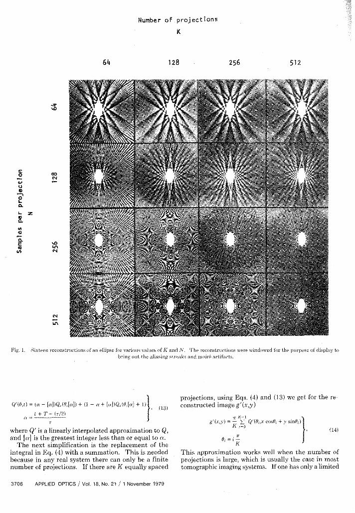
Sintecn reconstriictioiis of an ellipse fo~ . varioiis virlues of K kind ,\I. 'The rec<,nstriict.ioiis were windiwrd for thc piirpose or display l o bring oni, the aliasing slreaki and moire iirtiftict,~.

I projections, using Eqs. (4) and (13) we get for the re- W'(11,t) = (. - [irl)B,~(H,lnl) + (1 - n + /aj)Ws(fJ,[~r] + I ) , (lC3) constructed image g'(x,y

t + 7' - (7/2) <Y = K - - I

T xr(x,y) = - Q'(O, ,x cos8, + y sin0,) K ,-o

where Q' is a linearly interpolated approximation to Q, (14)

and [n] is the greatest integer less than or equal to ru. ii O , = i -

The next simplification is the replacement of the K

integral in Eq. (4) with a summation. This is needed This approximation works well when the number of 1)ei:ause in any real system there can only he a finite projections is large, which is usually the case in most number of projections. If there are K equally spaced tomographic imaging systems. If one has only alimited

3706 APPLIED OPTICS / Vol. 18. No. 21 / 1 November 1979

niimher of projections there may be better approxi- mations."

li:quation (14) is valid for any point (x,y), hut only a finite number of picture points can he reconstructed in ;I computer implementation. Since the picture is zero <,utside of a circle of radius T only a square ol dimen- sions 2T by 2Twill be considered. This will be sampled at MQoints. The discrete reconstructed image, de- noted by g,, is then related togf(x,y) as follows:

where 6 = (2T)lM. In summary, these approximations have been made:

the projections are spatially limited and bandlimited; the filtered projections can be recovered using linear interpolation; a finite number of projections can he used to make an accurate reconstruction; and the final image can be represented by a finite number of points.

I l l . Effects of the Approximations Figure I shows sixteen windowed reconstructions of

an ellipse with various values of K (number of projec- tions) and N (number of samples per projection). Figure 2 is a graphical depiction of the numerical values on the middle horizontal lines through two of the re- constructions. The following degradations are evident: Gibbs phenomenon, streaks, and moire patterns. These effects will now he related to the approximations made in the previous section.

A fundamental problem with these images and in general any tomographic pictures is that usually the ohjects are not bandlimited. When a nonbandlimited

function is sampletl or when a bandlimited function is sampled below its Nyquist rate, the portion of the spectrum above the Nyquist frequency is folded back into the lower frequencies. This causes the function to he bandlimited and also have aliasing errors in it.

Hackprojection is a linear process so the final image can be thought to be made up of two functions. One is the image made from the handlimited projections de- graded by linear interpolation and the finite number of projections. The second is the image made from the aliased portion of the spectrum in each projection.

The aliased portion of the reconstruction can be seen by itself by subtracting the transforms of the sampled projections from the corresponding theoretical trans- forms of the original projections. Then if this result is filtered as before the final reconstructed image will be that of the folded over spectrum. We performed a computer simulation study along these lines for an el- liptical object. In order to present the result of this study we first show in Fig. 3(a) the reconstruction of an ellipse for N = 64. (The number of projections was 51 2 and will remain the same tor the discussion here.) We subtracted the transform of each projection for the N = 64 case from the corresponding transform for N = 1024 case. The latter was assumed to be the true transform because the projections are oversampled (at least in comparisorl with the N = 64 case). The re- construction obtained from the difference data is shown in Fig. 3(h). Figure 3(c) is the bandlimited image ob- tained by suhtracting the aliased spectrum image of Fig. :i(b) from the complete image shown in Fig. 3(a). Fig- ure 3(c) is the reconstruction that would be obtained provided the projection data for the N = 64 case were truly band-limited (i.e., did not suffer from aliasing errors after sampling). The aliased-spectrum recon-

. O . i O E / 8 .O.LOO -I.ooe -oh" -O Loo -0.5m D obno ozmo a .&oo o l s o o i .aooo -$ .Lo+ - 0 h -0. bo -o.im ooboo o.&a i.$oo o . hoa !.dope

Fig. 2. 'Phis figure is a graphical depiction oi'the numerical values on the middle horizonial lines in two of the reconslrudions in Pig. 1. The jagged lines are the reconstrucled valr~es while the straight lines are the true values: (a) N = 64, K = 512; (b) N = 512, K = 512.

1 November 1979 / Vol. 18, No. 21 / APPLIED OPTICS 3707

Fig. 8. (a) Reconstruction of an ellipse with N = $4 and K = 512. (h) lieconstruction Crom only the aiiased frequencies in each projection. Note that the streaks exactly match those in (a). (c) Image obt.ained by subtracting (b) from (a). This is thc rrconstrtiction that, would hi,

obtained provided the data for the N = 64 cave were truly bandlimited.

struction in Fig. 3(b) and the absence of streaks in Fig. 3(c) prove our point that when the number of projec- tions is large, the streaking artifacts are caused by ali- asing errors in the projection data.

Imaging systems are often characterized by their point spread functions (PSF). For linear position- invariant systems such a characterization is generally considered to be complete. However, for sampled systems this is not always true. Often the PSF will give no indication of object-spectra dependent artifacts such as the aliasing streaks discussed above. For example, for the K = 512, N = 64 case, the PSF is shown in Fig. 4(b), while the reconstruction of the ellipse for the same K and N is shown in the upper right-hand corner of Fig. 1. While the PSF looks nice and smooth, the aliasing streaks are quite evident in the ellipse reconstruction. [The PSFs in Fig. 4 were generated for a point source located a t the origin. Also, for each projection the (N/2)th ray passed through the origin.]

The distortions that one can see in the PSF are those that are totally intrinsic to the algorithm such as would be caused by an inadequate number of projections, the effect of interpolation (which like aliasing depends upon N), and the display grid not being fine enough.

The system will yield perfect images (in the absence of aliasing) if the PSF has a single value at the origin and zero everywhere else. Because of the finite bandwidth, if K is infinite, the PSF will be the inverse Hankel transform of a disk of radius I?. That is, the PSF, de- noted by h(x,y), will now be given by the function

where r = (x' + y2)'/'. Clearly, the width of the main lobe is inversely related to the projection bandwidth R. This is also illustrated in Fig. 4 where the PSF for the N = 64 case has a wider main lobe than that for the N = 512.

Along with the main lobes, other structured noise can also he seen in some of the PSFs in Fig. 4. Brooks6 has shown that this noise is caused by a finite K. He also showed that if K is larger than [(1.11~)/4] N, the PSF is essentially noise free. This is confirmed in Fig. 4. It was shown by Shepp and Logan7 that for a finite K and infinite N the noise caused by the finite number of projections will go to infinity.

The effects of interpolation can he combined into the PSF. OppenheimQas shown that interpolation can he seen as convolving the unsampled projection with a window. Thus by the Fourier slice theorem, the Fourier transform of the PSF without interpolation is multi- plied by the Fourier transform of the window rotated about the origin. The PSFs presented in Fig. 4 already include the effects of interpolation. Because dilferent interpolation windows effect the spectrum differently, they could enhance or suppress the aliasing errors. This has led some authorsg to attribute aliasing streaks to interpolation errors.

The last degradation in the images is moirG pat- terns.'" These can be seen in Fig. 1 where N = 512 and K = 64. The projection data now have a large band- width. However, the display grid is not fine enough to represent these high frequencies and 2-D aliasing takes place. It is interesting to note that two different types of aliasing artifacts may occur in computerized tomog-

3708 APPLIED OPTICS / Vol. 18. No. 21 / 1 November 1979

(c ) ( d )

F~K. 4. Point functions for some of the reconstructions in Fig. 1

Fig. 5. (a) A symbolic depiction of the aliasing dist,<trt,ioi~. S(H,f) is the transforni of the trilc projec_lion at angle fl. (11) Stme ul't.he replicatic,ri oSS(f1.f) are siiowii here. The sixii oi'thcsc replicalioni is S(0.f).

1 November 1979 / Voi. 18, No. 21 / APPLIED OPTICS 3700

raphy: those caused by undersampling of the projec- Using the Fourier slice theorem and Parseval's theorem, tion data and those caused by the display grid not being Eq. (19) becomes fine enough.

IV. Upper Bound for Energy in Aliasing Streaks E A = A* ISA(O.f)lilfldfdO (20)

In this section an upper bound for the energy in the streaks for an elliptical object will he found assuming Since we are interested in aliased frequencies within the

an infinite number of projections. Our interest in el- measurement hand we may write

liptical objects stems from the mathematical tractability of this case and, also, because of their frequent use in E A = ArJ: ISA(O.f)lZIfIdfdO (21) computer simulation work in tomography.

Let S(O,f) be the Fourier transform of the samples of N~~ an object consisting of a single ellipse at the or- the projection at angle 0. I t is related to the true igin of major and minor axes given 2R and 2S, re- transform by spectively, is mathematically described by

- S(0.f) = f S(8,f - ZLB),

,=-- (17)

where B = '127, T being the sampling interval. Note that with the sampling interval 7, B the measurement bandwidth of the system. Both S(0,f) and S(0,f) are illustrated in Fig. 5. For most cases of aliasing distor- tion the measurement bandwidth R is only slightly less than the projection bandwidth W, which is the case depicted in the figure. Now let SA(O,f) denote the ali- ased frequency components within the measurement handwidth. It is clear from Fig. 5 that SA(B,f) consists essentially of contributions made by the two, the first left and the first right, replications of the baseband spectrum. Thus we may write

Let g A ( x , y ) denote the reconstruction from only the aliased frequencies. The total energy in this recon- struction will he denoted by E A and may be defined as

= 0, elsewhere (22)

The projections, P(O,t), of this object are given by

where a 2 = N 2 cos2B + S2 sin20. The Fourier transform of P(0,t) is given by

RSJi(2aaf ) S(0,f) = -- .

i (24)

where J1(.) is the Bessel function of order one. Near f = B a n d f = -R the function [ J ~ ( x ) ] l x can be

well approximated by its asymptotic form:

. . o D l l / ~ ~ - . r - ~ ~ ~ r~-~-. . 1. ..O. I .... PO a .oo0. n..... n...o* I..... nn... m.oo.0 93e.0

r/eq"<"/" ( 9 , . Fig. 6. This figure illustrates the fact that beyond the limits of the measurement bandwidth iri the frequency domain, the Rcssel function can be well approximated by its asymptotic form. (In this case the measiirement band is from f = -16 to f = 16) ?'he solid ciirve corresponds

to the exact result obtained by using Eq. (24); and the dashed curve is based on the approximation in Eq. (25).

3710 APPLIED OPTICS / Vol. 18. No. 21 / 1 November 1979

To illustrate the reasonableness of this approximation consider the case of the ellipse in Pig. 3 whose dimen- sions are given by R = 0 2 and S = 0.1. Now let us select

= 0.1 since this corresponds to the projection with the maximum bandwidth. Let us say we have 64 samples per projection and let the value of T be 1. Therefore, 7 = 2/64 and H = ST = 16. Hence the measurement band is given by -16 < f < 16. The solid curve in Fig. 6 is a plot of S(0 , f ) as given by Eq. (24) for 16 < f < 32; and the dashed curve is obtained hy using the approx- imation in (25). Since in our experiments the 64 sam- ples represent a highly undersanipled case, and since the asympt,otic approximation gets better as N is increased, using (25) is a good approximation for discussing ali- asing. Using (24) and (25) we write for s ( f - 2R) at I'requencies f < A:

for f < H. (26)

A similar asymptotic expression can be written for S(/ + 2B) at frequencies f > -R:

RS cos ~%nal.'H + f ) - -- S(8,f + 2 B ) =

n[a(2H + f ) ] : ' /2

for i > - H . (27)

We will now assume that the measurement bandwidth is large enough so that in the baseband spectrum frequencies above 2A do not contribute to aliasing. That is, for practical purposes we may write B < W < 2B. [Note that this assumption is consistent with ours including only two replications in Eq. (181.1 Therefore, we can ignore the energy in S(0,f - 2R) and S(H,f + 2R) at frequencies f < 0 and f > 0, respectively. With this assumption substitution of (26) and (27) in (18) leads

Substituting Eq. (28) into Eq. (21)

(29)

The inner integral can be reduced to

The integral in (30) can he hounded in ahsolute value by 1/(4H) so the integral in (29) reduces to

The integral in (31) can be evaluated using identities found in Ref. 11.

R E X < - - E ii?i. (32

lr ZH

where 0 = (1 - (S /R )2 )1 /2 and where E [ x ] is an elliptic integral defined as

hyX] = J" ( 1 - x 2 sln . 2 n)'t2dor. 0

(33)

The value of the upper bound in (31) [or (32)] lies in its functional dependence on the parameters of the size of the ellipse. This upper bound led us to an interesting conclusion (verified eventually by computer simulation) that although a larger ellipse is more low-frequency in character, the enengy in its aliasing streaks should be greater. The intuitive justification for this is the fact that as an ellipse gets larger, in its frequency domain representation its energy increases at all frequencies including ihose that contribute to aliasing. The reader may note that for any give SIR as an ellipse is made larger, although E A increases, the normalized streak energy given by EAI?rRS will decrease. The factor ?rRS is the energy in the ellipse itself. Also (31) [or (3211 lead to the expected conclusion that the energy in the streaks is bounded from above by a function that is inversely related to the bandwidth, which implies that it is in- versely related to the number or sample points. This is seen in Fig. I in the last column where the streaks die out as N increases.

V. Conclusions

In computerized tomography based on filtered- backprojection algorithms, streaks are caused by ali- asing errors introduced when the projection data are undersampled. These aliasing streaks are different from (and, in addition to) the streaks caused by an in- sufficient number of projections.

This work was partly supported by the NIH grant GM24994-01

References 1 . R. N . Bracewell and A. C. Riddle, Astrophys J . 150, (1967). 2. A. C. Kak, "Computeri7,ed Tomography with X-ray, Emission

and Ultrasound Sources," to appear in Proc. IEEE 67, (Sept. 1979).

:i. A. C. Kak. C. V. Jakowatz, N. Haiiy, and I<. Keller, IEtZETrans. Hicsmed. Eng. BME-24, 157 (1977).

,i. (:. 11. Crawhrd and A. C. Kak, "Aliasing Artifacts in CT Irnagcs," Sch,,i,l 01' Electrical Enginccriiig, Purdue University, Research Iteport 'Tlt~lCl? 79-25 (Ilecemhrr 1978).

5. C. V, Jakowatz and A. C. Kak, "Computerizedl'omography Using X-rays and Ultrasound," School ofElectiica1 Engineering, Pur- due University, Rcsearch Report TR-Eb: 76-26, July 1976.

6. R. A. Brooks, C. H. Weiss, and A. J . Talhert, .I. Comput. Assisted Tomog. 12,577 (Nov. 1978).

7 . L. A. Shepp arid B. F. Logwn, Ib:EE Trans, h'iicl. Sci. NS-22.21 (June 1974).

8. H. I+:. Oppenheim, "Reconstruction Tomography from I!,cornplete l'rojections," in Reconstruction 'romography in Diagnostic Radiology and Nuclear Medicine, M . M. Ter-Pogossian, Ed. (University Park Press, University Park, Pa. 1977), pp, 155- 183.

9. H . P. Weiss and d. A. Stein, "The Effect of Interpolation in CT Image Reconstruction," in Proerrdings I E E E Conference on Pattprn Recognition and Image Processing, Chicago, May 1978, p. 193.

10. A. Rosenfeld and A. C. Kak, D i ~ i t a l PiLture Processing (Aca- dernic, New York, 1976).

11. I. S. Gradshteyn and I. M, Ryzhik, Table oiintrgrals, Series, and Products (Academic, New York, 1965), p 156.

1 November 1979 / Vo ! 18, No. 21 / APPLIED OPTICS 371 1