algorithms - nms.kcl.ac.uk
TRANSCRIPT

Algorithms
I What is an algorithm?
I Informally, an algorithm is a well-defined finite set of rulesthat specifies a sequential series of elementary operations tobe applied to some data called the input, producing after afinite amount of time some data called the output.
I The oldest non-trivial algorithm, that has survived to thepresent day, is the Euclidean algorithm, named after the Greekmathematician Euclid (fl. 300 BC), for computing thegreatest common divisor of two natural numbers.
I The word Algorithm derives from the name of a Persianmathematician al-Khwarizmi (c. 780 - c. 850).
I An algorithmic solution to a computational problem willusually involve designing an algorithm, and then analysingits performance.

Algorithms
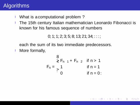
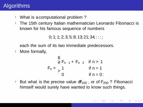
I What is a computational problem?
I The 15th century Italian mathematician Leonardo Fibonacci isknown for his famous sequence of numbers
0, 1, 1, 2, 3, 5, 8, 13, 21, 34, . . . ,
each the sum of its two immediate predecessors.
I More formally,
Fn =
Fn−1 + Fn−2 if n > 1
1 if n = 1
0 if n = 0.
I But what is the precise value of F100 , or of F200 ? Fibonaccihimself would surely have wanted to know such things.
I To answer, we need to design an algorithm for computingthe nth Fibonacci number.
Algorithms
I What is a computational problem?
I The 15th century Italian mathematician Leonardo Fibonacci isknown for his famous sequence of numbers
0, 1, 1, 2, 3, 5, 8, 13, 21, 34, . . . ,
each the sum of its two immediate predecessors.
I More formally,
Fn =
Fn−1 + Fn−2 if n > 1
1 if n = 1
0 if n = 0.
I But what is the precise value of F100 , or of F200 ? Fibonaccihimself would surely have wanted to know such things.
I To answer, we need to design an algorithm for computingthe nth Fibonacci number.
Algorithms
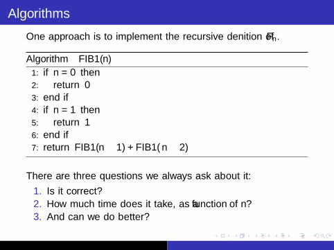
One approach is to implement the recursive definition of Fn.
Algorithm FIB1(n)
1: if n = 0 then2: return 03: end if4: if n = 1 then5: return 16: end if7: return FIB1(n − 1) + FIB1(n − 2)
There are three questions we always ask about it:
1. Is it correct?
2. How much time does it take, as a function of n?
3. And can we do better?
The algorithm is definitely correct. It is the definition of Fn.

Algorithms
One approach is to implement the recursive definition of Fn.
Algorithm FIB1(n)
1: if n = 0 then2: return 03: end if4: if n = 1 then5: return 16: end if7: return FIB1(n − 1) + FIB1(n − 2)
There are three questions we always ask about it:
1. Is it correct?
2. How much time does it take, as a function of n?
3. And can we do better?
The algorithm is definitely correct. It is the definition of Fn.

Recursive Fibonacci
The recursive calls of FIB(6)
From CLRS Introduction to Algorithms Chapter 27

Algorithms
How much time does FIB1(n) take, as a function of n?
I Let T (n) be the number of computer steps needed tocompute FIB1(n); what can we say about this function?
I For starters, if n is less than 2, the procedure halts almostimmediately, after just a couple of steps.
T (n) ≤ 2 for n ≤ 1.
I For larger values of n, there are two recursive invocations ofFIB1: one taking time T (n − 1) and one taking timeT (n − 2); plus three other steps (check the value of n and afinal addition).
T (n) = T (n − 1) + T (n − 2) + 3 for n > 1.

Algorithms
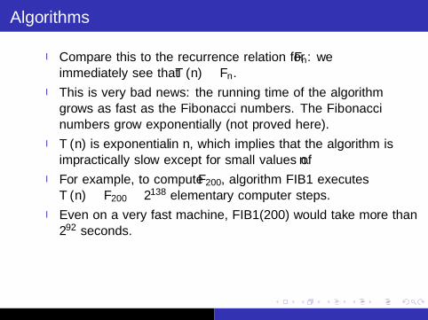
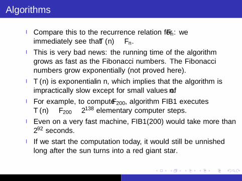
I Compare this to the recurrence relation for Fn: weimmediately see that T (n) ≥ Fn.
I This is very bad news: the running time of the algorithmgrows as fast as the Fibonacci numbers. The Fibonaccinumbers grow exponentially (not proved here).
I T (n) is exponential in n, which implies that the algorithm isimpractically slow except for small values of n.
I For example, to compute F200, algorithm FIB1 executesT (n) ≥ F200 ≥ 2138 elementary computer steps.
I Even on a very fast machine, FIB1(200) would take more than292 seconds.
I If we start the computation today, it would still be unfinishedlong after the sun turns into a red giant star.
I The algorithm is correct, but can we do better?

Algorithms
I Compare this to the recurrence relation for Fn: weimmediately see that T (n) ≥ Fn.
I This is very bad news: the running time of the algorithmgrows as fast as the Fibonacci numbers. The Fibonaccinumbers grow exponentially (not proved here).
I T (n) is exponential in n, which implies that the algorithm isimpractically slow except for small values of n.
I For example, to compute F200, algorithm FIB1 executesT (n) ≥ F200 ≥ 2138 elementary computer steps.
I Even on a very fast machine, FIB1(200) would take more than292 seconds.
I If we start the computation today, it would still be unfinishedlong after the sun turns into a red giant star.
I The algorithm is correct, but can we do better?

Algorithms
I A faster approach could be store the intermediate results: thevalues F0,F1, . . . ,Fn−1.
Algorithm FIB2(n)
1: if n ≤ 1 then2: return n3: end if4: f [0 . . . n]← 05: f [0]← 06: f [1]← 17: for all i ∈ [2, n] do8: f [i ]← f [i − 1] + f [i − 2]9: end for
10: return f [n]
I The correctness of this algorithm follows by definition of Fn.
Algorithm FIB2
I How long does it take?
I The for loop (lines 7-8) consists of a single computer step andis executed n − 1 times.
I Therefore the number of computer steps used by FIB2(n) islinear in n.
I From exponential we are down to polynomial, a hugebreakthrough in running time.
I It is now perfectly reasonable to compute F200 or evenF200,000.
Brief discussion
I What was the difference in design between these twoalgorithms?
I The second algorithm is faster than the first when run on asingle processor.
I The first algorithm is recursive, and used a divide-and-conquerapproach to split the problem into sub-problems
I The second algorithm is completely sequential, building Fnfrom our previous knowledge of Fn−1 and Fn−2.
I The sequential running time of the second algorithm is bestpossible (optimal).We need n steps to compute Fn.

Running time of Algorithms
I Instead of reporting that an algorithm takes, say, 5n3 + 4n + 3steps on an input of size n, it is much simpler to leave outlower-order terms such as 4n and 3 (which becomeinsignificant as n grows).
I Even the detail of the coefficient 5 in the leadingterm—computers will be five times faster in a few yearsanyway.
I We just say that the algorithm takes time O(n3) (pronounced“big oh of n3”).
I We define this notation precisely by thinking of f (n) and g(n)as the running times of two algorithms on inputs of size n.

Algorithms
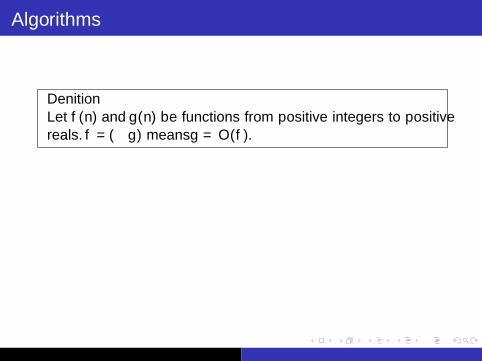
DefinitionLet f (n) and g(n) be functions from positive integers to positivereals. We say f = O(g) (which means that “f grows no fasterthan g”) if there is a constant c > 0 such that f (n) ≤ c .g(n).

Algorithms
I Saying f = O(g) is a very loose analog of f ≤ g .
I It differs from the usual notion of ≤ due to the constant c .
I This constant also allows us to disregard what happens forsmall values of n.
I Suppose f1(n) = n2 and f2(n) = 2n + 20. Which is better(smaller)?
I Well, this depends on the value of n. For n ≤ 5, f1 is smaller;thereafter, f2 is the clear winner.
I In this case, f2 scales much better as n grows, and therefore itis smaller.

Algorithms
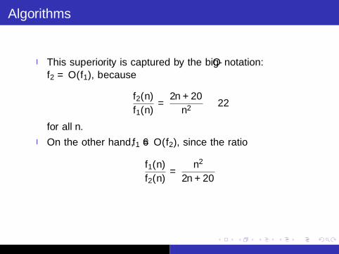
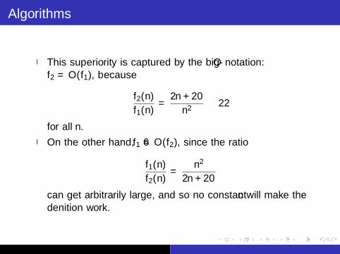
I This superiority is captured by the big-O notation:f2 = O(f1), because
f2(n)
f1(n)=
2n + 20
n2≤ 22
for all n.
I On the other hand, f1 6= O(f2), since the ratio
f1(n)
f2(n)=
n2
2n + 20
can get arbitrarily large, and so no constant c will make thedefinition work.

Algorithms
I This superiority is captured by the big-O notation:f2 = O(f1), because
f2(n)
f1(n)=
2n + 20
n2≤ 22
for all n.
I On the other hand, f1 6= O(f2), since the ratio
f1(n)
f2(n)=
n2
2n + 20
can get arbitrarily large, and so no constant c will make thedefinition work.

Algorithms
I This superiority is captured by the big-O notation:f2 = O(f1), because
f2(n)
f1(n)=
2n + 20
n2≤ 22
for all n.
I On the other hand, f1 6= O(f2), since the ratio
f1(n)
f2(n)=
n2
2n + 20
can get arbitrarily large, and so no constant c will make thedefinition work.

Algorithms
I This superiority is captured by the big-O notation:f2 = O(f1), because
f2(n)
f1(n)=
2n + 20
n2≤ 22
for all n.
I On the other hand, f1 6= O(f2), since the ratio
f1(n)
f2(n)=
n2
2n + 20
can get arbitrarily large, and so no constant c will make thedefinition work.
Algorithms
I This superiority is captured by the big-O notation:f2 = O(f1), because
f2(n)
f1(n)=
2n + 20
n2≤ 22
for all n.
I On the other hand, f1 6= O(f2), since the ratio
f1(n)
f2(n)=
n2
2n + 20
can get arbitrarily large, and so no constant c will make thedefinition work.
Algorithms
I This superiority is captured by the big-O notation:f2 = O(f1), because
f2(n)
f1(n)=
2n + 20
n2≤ 22
for all n.
I On the other hand, f1 6= O(f2), since the ratio
f1(n)
f2(n)=
n2
2n + 20
can get arbitrarily large, and so no constant c will make thedefinition work.

Algorithms
2n + 20 = O(n2)

Algorithms
2n + 20 = O(n2)

Algorithms
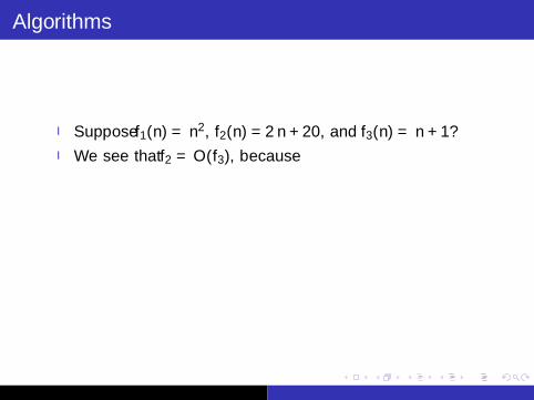
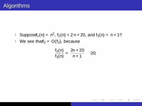
I Suppose f1(n) = n2, f2(n) = 2n + 20, and f3(n) = n + 1?
I We see that f2 = O(f3), because
f2(n)
f3(n)=
2n + 20
n + 1≤ 20,
but also f3 = O(f2), this time with c = 1.
I Just as O(.) is an analog of ≤ we can also define analogs of≥ and = as follows.

Algorithms
I Suppose f1(n) = n2, f2(n) = 2n + 20, and f3(n) = n + 1?
I We see that f2 = O(f3), because
f2(n)
f3(n)=
2n + 20
n + 1≤ 20,
but also f3 = O(f2), this time with c = 1.
I Just as O(.) is an analog of ≤ we can also define analogs of≥ and = as follows.
Algorithms
I Suppose f1(n) = n2, f2(n) = 2n + 20, and f3(n) = n + 1?
I We see that f2 = O(f3), because
f2(n)
f3(n)=
2n + 20
n + 1≤ 20,
but also f3 = O(f2), this time with c = 1.
I Just as O(.) is an analog of ≤ we can also define analogs of≥ and = as follows.
Algorithms
I Suppose f1(n) = n2, f2(n) = 2n + 20, and f3(n) = n + 1?
I We see that f2 = O(f3), because
f2(n)
f3(n)=
2n + 20
n + 1≤ 20,
but also f3 = O(f2), this time with c = 1.
I Just as O(.) is an analog of ≤ we can also define analogs of≥ and = as follows.

Algorithms
I Suppose f1(n) = n2, f2(n) = 2n + 20, and f3(n) = n + 1?
I We see that f2 = O(f3), because
f2(n)
f3(n)=
2n + 20
n + 1≤ 20,
but also f3 = O(f2), this time with c = 1.
I Just as O(.) is an analog of ≤ we can also define analogs of≥ and = as follows.

Algorithms
I Suppose f1(n) = n2, f2(n) = 2n + 20, and f3(n) = n + 1?
I We see that f2 = O(f3), because
f2(n)
f3(n)=
2n + 20
n + 1≤ 20,
but also f3 = O(f2), this time with c = 1.
I Just as O(.) is an analog of ≤ we can also define analogs of≥ and = as follows.
Algorithms
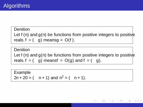
DefinitionLet f (n) and g(n) be functions from positive integers to positivereals. f = Ω(g) means g = O(f ).
DefinitionLet f (n) and g(n) be functions from positive integers to positivereals. f = Θ(g) means f = O(g) and f = Ω(g).
Example2n + 20 = Θ(n + 1) and n2 = Ω(n + 1).
Algorithms
DefinitionLet f (n) and g(n) be functions from positive integers to positivereals. f = Ω(g) means g = O(f ).
DefinitionLet f (n) and g(n) be functions from positive integers to positivereals. f = Θ(g) means f = O(g) and f = Ω(g).
Example2n + 20 = Θ(n + 1) and n2 = Ω(n + 1).

Algorithms
DefinitionLet f (n) and g(n) be functions from positive integers to positivereals. f = Ω(g) means g = O(f ).
DefinitionLet f (n) and g(n) be functions from positive integers to positivereals. f = Θ(g) means f = O(g) and f = Ω(g).
Example2n + 20 = Θ(n + 1) and n2 = Ω(n + 1).
Algorithms
DefinitionLet f (n) and g(n) be functions from positive integers to positivereals. f = Ω(g) means g = O(f ).
DefinitionLet f (n) and g(n) be functions from positive integers to positivereals. f = Θ(g) means f = O(g) and f = Ω(g).
Example2n + 20 = Θ(n + 1) and n2 = Ω(n + 1).

Algorithms
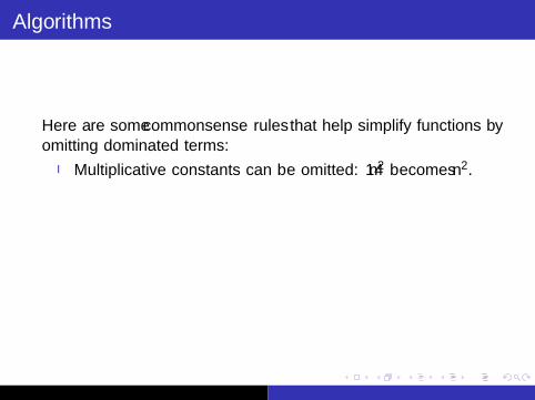
Here are some commonsense rules that help simplify functions byomitting dominated terms:
I Multiplicative constants can be omitted: 14n2 becomes n2.
I na dominates nb if a > b: for instance, n2 dominates n.
I Any exponential dominates any polynomial: 3n dominates n5.
I Likewise, any polynomial dominates any logarithm: ndominates (log n)3. This also means, for example, that n2
dominates n log n.
Algorithms
Here are some commonsense rules that help simplify functions byomitting dominated terms:
I Multiplicative constants can be omitted: 14n2 becomes n2.
I na dominates nb if a > b: for instance, n2 dominates n.
I Any exponential dominates any polynomial: 3n dominates n5.
I Likewise, any polynomial dominates any logarithm: ndominates (log n)3. This also means, for example, that n2
dominates n log n.

Parallel Algorithms: What?
Devising algorithms which allow many processors to workcollectively to solve:
I the same problems, but faster
I bigger/more refined problems in the same time
when compared to a single processor.
Parallel Algorithms: What?
Devising algorithms which allow many processors to workcollectively to solve:
I the same problems, but faster
I bigger/more refined problems in the same time
when compared to a single processor.
Parallel Algorithms: What?
Devising algorithms which allow many processors to workcollectively to solve:
I the same problems, but faster
I bigger/more refined problems in the same time
when compared to a single processor.

Parallel Algorithms: What?
Devising algorithms which allow many processors to workcollectively to solve:
I the same problems, but faster
I bigger/more refined problems in the same time
when compared to a single processor.

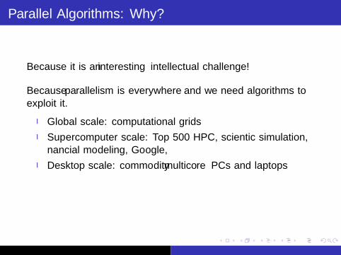
Parallel Algorithms: Why?
Because it is an interesting intellectual challenge!
Because parallelism is everywhere and we need algorithms toexploit it.
I Global scale: computational grids
I Supercomputer scale: Top 500 HPC, scientific simulation,financial modeling, Google,
I Desktop scale: commodity multicore PCs and laptops
I Specialised hardware: custom parallel circuits for keyoperations such as encryption, and multimedia (NVIDIA)

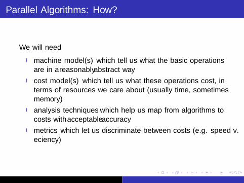
Parallel Algorithms: How?
We will need
I machine model(s) which tell us what the basic operationsare in a reasonably abstract way
I cost model(s) which tell us what these operations cost, interms of resources we care about (usually time, sometimesmemory)
I analysis techniques which help us map from algorithms tocosts with acceptable accuracy
I metrics which let us discriminate between costs (e.g. speed v.efficiency)
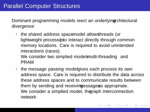
Parallel Computer Structures
Dominant programming models reflect an underlying architecturaldivergence:
I the shared address space model allows threads (orlightweight processes) to interact directly through commonmemory locations. Care is required to avoid unintendedinteractions (races).We consider two simplified models multi-threading andPRAM
I the message passing model gives each process its ownaddress space. Care is required to distribute the data acrossthese address spaces and to communicate results betweenthem by sending and receiving messages as appropriate.We consider a simplified model, the graph interconnectionnetwork

Parallel Computer Structures
Dominant programming models reflect an underlying architecturaldivergence:
I the shared address space model allows threads (orlightweight processes) to interact directly through commonmemory locations. Care is required to avoid unintendedinteractions (races).
We consider two simplified models multi-threading andPRAM
I the message passing model gives each process its ownaddress space. Care is required to distribute the data acrossthese address spaces and to communicate results betweenthem by sending and receiving messages as appropriate.We consider a simplified model, the graph interconnectionnetwork

Parallel Computer Structures
Dominant programming models reflect an underlying architecturaldivergence:
I the shared address space model allows threads (orlightweight processes) to interact directly through commonmemory locations. Care is required to avoid unintendedinteractions (races).We consider two simplified models multi-threading andPRAM
I the message passing model gives each process its ownaddress space. Care is required to distribute the data acrossthese address spaces and to communicate results betweenthem by sending and receiving messages as appropriate.We consider a simplified model, the graph interconnectionnetwork

Parallel Computer Structures
Dominant programming models reflect an underlying architecturaldivergence:
I the shared address space model allows threads (orlightweight processes) to interact directly through commonmemory locations. Care is required to avoid unintendedinteractions (races).We consider two simplified models multi-threading andPRAM
I the message passing model gives each process its ownaddress space. Care is required to distribute the data acrossthese address spaces and to communicate results betweenthem by sending and receiving messages as appropriate.
We consider a simplified model, the graph interconnectionnetwork
Parallel Computer Structures
Dominant programming models reflect an underlying architecturaldivergence:
I the shared address space model allows threads (orlightweight processes) to interact directly through commonmemory locations. Care is required to avoid unintendedinteractions (races).We consider two simplified models multi-threading andPRAM
I the message passing model gives each process its ownaddress space. Care is required to distribute the data acrossthese address spaces and to communicate results betweenthem by sending and receiving messages as appropriate.We consider a simplified model, the graph interconnectionnetwork

Multi-threading model
High level model of thread processes using spawn and sync.Does not consider the underlying hardware.
Algorithm Algorithm-A
begin· · · spawn Algorithm-Bdo Algorithm-B in parallel with this code· · · other stuff · · · syncwait here for all previous spawned parallel computations to complete· · · end
Multi-threading model
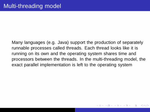
Many languages (e.g. Java) support the production of separatelyrunnable processes called threads. Each thread looks like it isrunning on its own and the operating system shares time andprocessors between the threads. In the multi-threading model, theexact parallel implementation is left to the operating system

PRAM model
The processors act synchronouslySIMD (single instruction multiple data)Several read-write possibilities (exclusive-concurrent)Any mix of ER, EW, CR, CW, e.g. EREWEREW algorithms can be very different from CRCW
Interconnection network
Graph G = (V ,E )Each node i in V is a processor Pi
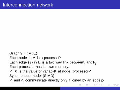
Each edge (i , j) in E is a two way link between Pi and Pj
Each processor has its own memory.P · X is the value of variable X at node (processor) PSynchronous model (SIMD)Pi and Pj communicate directly only if joined by an edge (i , j)
Concluding remarks and examples
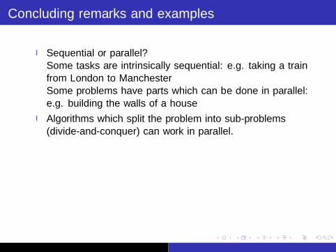
I Sequential or parallel?Some tasks are intrinsically sequential: e.g. taking a trainfrom London to ManchesterSome problems have parts which can be done in parallel:e.g. building the walls of a house
I Algorithms which split the problem into sub-problems(divide-and-conquer) can work in parallel.
I Parallel or Distributed?
I In both cases many processors run the same program.A parallel system has a central controller. All processorsexecute the same step of the program at the same timeA distributed system has no central control. Processorscooperate to obtain a well regulated system

Concluding remarks and examples
I Sequential or parallel?Some tasks are intrinsically sequential: e.g. taking a trainfrom London to ManchesterSome problems have parts which can be done in parallel:e.g. building the walls of a house
I Algorithms which split the problem into sub-problems(divide-and-conquer) can work in parallel.
I Parallel or Distributed?
I In both cases many processors run the same program.A parallel system has a central controller. All processorsexecute the same step of the program at the same timeA distributed system has no central control. Processorscooperate to obtain a well regulated system
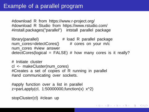
Example of a parallel program
#download R from https://www.r-project.org/#download R Studio from https://www.rstudio.com/#install.packages("parallel") intstall parallel package
library(parallel) # load R parallel packagenum_cores=detectCores() # cores on your m/cnum_cores #view answerdetectCores(logical = FALSE) # how many cores is it really?
# Initiate clustercl <- makeCluster(num_cores)#Creates a set of copies of R running in parallel#and communicating over sockets.
#apply function over a list in parallelz=parLapply(cl, 1:50000000,function(x) x^2)
stopCluster(cl) #clean up

Task manager snapshot
Rainfall prediction
An international team led by Takemasa Miyoshi of the RIKEN Advanced Center for Computational Science (AICS)has used the powerful K computer and advanced radar observational data to accurately predict the occurrence oftorrential rains in localized areas.Today, supercomputer-based weather predictions are typically done with simulations that use grids spaced at leastone kilometer apart, and incorporate new observational data every hour. However, due to the roughness of thecalculations, these simulations cannot accurately predict the threat of torrential rains, which can develop withinminutes when cumulonimbus clouds suddenly develop. Now, an international team led by Takemasa Miyoshi of theRIKEN Advanced Center for Computational Science (AICS) has used the powerful K computer and advanced radarobservational data to accurately predict the occurrence of torrential rains in localized areas.The key to the current work, to be published later this month in the August issue of the Bulletin of the AmericanMeteorological Society, is ”big data assimilation” using computational power to synchronize data betweenlarge-scale computer simulations and observational data.Using the K computer, the researchers carried out 100 parallel simulations of a convective weather system, usingthe nonhydrostatic mesoscale model used by the Japan Meteorological Agency, but with 100-meter grid spacingrather than the typical 2-kilometer or 5-kilometer spacing, and assimilated data from a next-generation phasedarray weather radar, which was launched in the summer of 2012 by the National Institute of Information andCommunications Technology (NICT) and Osaka University. With this, they produced a high-resolutionthree-dimensional distribution map of rain every 30 seconds, 120 times more rapidly than the typical hourlyupdated systems operated at the world’s weather prediction centers today.To test the accuracy of the system, the researchers attempted to model a real case – a sudden storm that tookplace on July 13, 2013 in Kyoto, close enough to Osaka that it was caught by the radars at Osaka University. Thesimulations were run starting at 15:00 Japanese time, and were tested as pure simulations without observationaldata input as well as with the incorporation of data every 30 seconds, on 100-meter and 1-kilometer grid scales.The simulation alone was unable to replicate the rain, while the incorporation of observational data allowed thecomputer to represent the actual storm. In particular, the simulation done with 100-meter grids led to a veryaccurate replication of the storm compared to actual observations.According to Miyoshi, ”Supercomputers are becoming more and more powerful, and are allowing us to incorporateever more advanced data into simulations. Our study shows that in the future, it will be possible to use weatherforecasting to predict severe local weather phenomena such as torrential rains, a growing problem which can causeenormous damage and cost lives.”


Thats the end of the introduction!
Bibliography I
The materials for this lecture were taken and partially adaptedfrom:
I “Algorithms” by S. Dasgupta, C. H. Papadimitriou, and U. V.Vazirani. McGraw-Hill
I “Introduction to Parallel Computing” by Ananth Grama,George Karypis, Vipin Kumar, and Anshul Gupta. Pearson
I “Design and Analysis of Parallel Algorithms” Course Slides byMurray Cole, School of Informatics, University of Edinburgh.
I CLRS, Introduction to Algorithms Chapter 27 (downloaded)
I Various articles from WWW