algorithms lecture notes - hendrix college
TRANSCRIPT

Algorithms Lecture Notes
Brent Yorgey
October 19, 2019
These are my lecture notes for CSCI 280 / CSCI 382, Algorithms, at HendrixCollege. Much of the basis for the course (including some of the lecture notesthemselves) came from a similar course taught by Brent Heeringa at WilliamsCollege.
There are two “tracks”: a “traditional” lecture-based version that I taughtin S’16 and S’17, and a revamped version which is a hybrid between lecture andPOGIL activities (http://pogil.org). I have left them both here for posterityand also because I may move material back and forth between them in thefuture. Sections marked with (L*) were used only in the lecture-based versionof the course; sections marked with (P*) only in the POGIL version; sectionsmarked with (L/P) are used in both, but presented via a POGIL activity ratherthan lecture; sections marked (L) are presented via lecture in both. Contact meif you would like to receive the latest versions of the POGIL activities I havedeveloped.
1

1 (P*) Introduction to POGIL and Algorithms
2

2 (P*) GCD analysis
3

3 (P*) Proving the Euclidean Algorithm correct
Here are the two algorithms we considered last time. Throughout the followingwe assume that a, b ≥ 0.
GCDI(a,b) =while (b 6= 0) and (a 6= 0)
if a ≤ bthen b← b mod aelse a← a mod b
if a = 0 then return b else return a
GCDR(a,b) =if b = 0
then aelse GCDR(b, a mod b)
How can we formally prove that these algorithms correctly compute the GCDof two nonnegative integers?
In proving either of these algorithms (or any algorithm) correct we reallyhave two things to prove:
1. The algorithm always terminates (stops in a finite amount of time) forany inputs.
2. If the algorithm does terminate, it returns the correct answer.
Sometimes the fact that the algorithm terminates is obvious; but in this case itdoes require some proof. It often makes things simpler to break up a proof ofcorrectness in this way.
We’ll start with the recursive version; it’s typically easier to prove thingsabout recursive algorithms than iterative ones.
Theorem 3.1. GCDR(a, b) always terminates.
Proof. By (strong) induction on b.
• If b = 0, GCDR(a, b) = a.
• Otherwise, if b > 0, GCDR makes a recursive call to GCDR(b, a mod b).This is well-defined since b 6= 0. By definition 0 ≤ a mod b < b, so thesecond argument to the recursive call is strictly smaller than b. Hence, bythe induction hypothesis, that recursive call must terminate.
Put more informally, the second argument gets strictly smaller with everyrecursive call. It cannot keep getting smaller forever; it must eventuallyreach the base case of 0 and stop. SDG
Now, in order to prove that GCDR is correct, we first need a small lemmaabout the mathematical gcd function. Note carefully the difference betweenGCDR, GCDI, and gcd: the former two refer to the particular algorithms definedby the code above, whereas gcd refers to the abstract mathematical functiondefined in terms of divisors and so on. gcd is a specification whereas GCDRand GCDI are implementations; our job is to prove that they actually produceidentical results, that is, that the implementations match the specification.
4

Lemma 3.2. If b 6= 0 then gcd(a, b) = gcd(a mod b, b).
Proof. The proof uses some basic number theory. I typically skip it since we’remore interested in the algorithmic aspects of the proof. However, the proof isincluded here in the notes for completeness.
It suffices to prove that for any d > 0, d evenly divides both a and b if andonly if it evenly divides (a mod b) and b. Then (a, b) and (a mod b, b) have thesame set of common divisors, and hence the same greatest common divisor.
Note that a mod b = a− kb for some constant k. If d divides a and b then italso divides kb and therefore a− kb. Conversely, suppose some e divides both band a−kb. Then e divides kb, and hence it divides the sum (a−kb)+kb = a. SDG
Theorem 3.3. GCDR(a, b) = gcd(a, b).
Proof. By induction on b.
• In the base case, when b = 0, GCDR(a, 0) = a, which is indeed the defini-tion of gcd(a, 0).
• Now suppose b > 0 and that for all a, GCDR(a, b′) = gcd(a, b′) when-ever b′ < b. In this case GCDR(a, b) = GCDR(b, a mod b). We knowa mod b < b, so the induction hypothesis applies (note in particular thatthe IH holds for any a, and in particular we can pick b as our “a”).We concude that GCDR(a, b) = GCDR(b, a mod b) = gcd(b, a mod b) =gcd(a mod b, b) = gcd(a, b), where the last two steps follow from the factthat gcd is symmetric (easily deduced from its definition) and the previouslemma. SDG
Now we’ll prove the iterative algorithm correct, beginning with termination.
Theorem 3.4. GCDI(a, b) always terminates.
Proof. Each time through the loop, either a gets smaller and b stays the same, orb gets smaller and a stays the same: if the loop starts out with a ≤ b, then b getssmaller, since b mod a < a ≤ b. Otherwise a gets smaller, since a mod b < b < a.Since neither ever gets bigger and one gets strictly smaller every loop iteration,one of them must eventually hit 0, which will stop the loop.1 SDG
Theorem 3.5. GCDI(a, b) = gcd(a, b).
Proof. Suppose we initially call GCDI(m,n). Then we claim the following loopinvariant : each time right before doing the loop check again, gcd(a, b) = gcd(m,n).That is, the gcd of the current values of a and b is always equal to the gcd ofthe original arguments to GCDI.
We prove this by induction on the number of loop executions.
• In the base case, before the loop has executed at all, a and b are equal tothe original arguments to GCDI, hence the invariant holds trivially.
1Technically this is a proof by (well-founded) induction on pairs N2 under the well-foundedrelation (a, b) < (x, y) if a < x and b = y or a = x and b < y.
5

• Otherwise, suppose the invariant held after n loop iterations; we mustshow it will still hold after one more loop iteration. But this follows fromLemma 3.2.
Finally, after the loop ends, we will have either a = 0 or b = 0, and we cansee that we will return wichever one is nonzero. This correctly returns the gcdof a and b since gcd(a, 0) = a. But because of the loop invariant we know thatgcd(a, b) = gcd(m,n), hence GCDI(m,n) = gcd(m,n). SDG
6

4 (L*) Stable matchings and Gale-Shapley
Administrivia
• Show course webpage.
• Weekly HW, due Fri 4pm. (See short HW due this Friday!!) Solutionshanded out Wednesday.
• Collaboration but separate write-up. I take academic integrity very seri-ously.
• 2 midterms and a final—given problems ahead of time, come in and writesolutions.
• Explain office hours, youcanbook.me, email habits.
Course goals
What is this course all about? Two main things:
1. Solving problems: learning techniques, skills, methods, common problemsand solutions, etc.
2. Proving that our solutions are good (correct, fast, low memory, etc.)
Connecting theory and practice!
Stable matching problem
Input:
• n doctors A = a1, . . . , an
• n hospitals with a slot for a resident B = b1, . . . , bn
• Rank lists: each doctor has a list of all hospitals in preferred order, andeach hospital has a list of doctors.
Example:
• Doctors x, y, z
• Hospitals MGH, Mayo, ACH
• Rank lists:
x MGH Mayo ACHy ACH MGH Mayoz Mayo MGH ACH
MGH z x yMayo y x zACH y z x
7

Goal: match up doctors and hospitals so no one wants to swap. That is, forany given doctor d and hospital h, either:
• d and h are matched, or
• d prefers their current hospital over h, or
• h prefers their current doctor over d.
So d and h don’t want to both abandon their current match and switch to eachother. This kind of matching where no one wants to swap is called stable.
• Example of stable matching: x—MGH, y—ACH, z—Mayo.
• Example of unstable matching: x—Mayo, y—MGH, z—ACH. Note thatx prefers MGH over Mayo, and MGH prefers x over y.
How long would a brute-force solution take?
• List every possible matching (n!)
• Check each matching to see if it is stable
– Check every pair of doctor & hospital (n2)
So something like O(n2n!), yikes.
The Gale-Shapley algorithm
Historically this has been called the stable marriage problem, phrased in termsof men & women pairing off. Studied by Gale and Shapley (1962), who gavethe following algorithm. This algorithm (a variant of it) is actually used by theNational Resident Matching Program to match residents and hospitals.
Algorithm 1 Propose-Reject - finds a stable matching
1: Initialize each proposer p and accepter a as Free2: while there is a free proposer who hasn’t proposed to every accepter do3: Choose a free proposer p4: a ← first accepter on p’s list to whom p has not yet proposed5: if a is Free then6: p and a are Matched (for now)7: else if a prefers p to their current match p′ then8: p and a are Matched and p′ is Free9: else
10: a rejects p and p remains Free
Pick two volunteers to be algorithm masters—job is to make sure algorithmis being correctly followed. Then split remaining students into 2 equal groups(add myself if an odd number), doctors and hospitals.
8

• Hospitals will have a letter. Have each doctor make up a ranking ofhospital letters.
• Have each hospital make up a ranking of numbers.
• Now randomly assign letters and numbers. Write assignments up on theboard so everyone can write down names next to their ranking.
• On your piece of paper:
– Your ranking
– Your identity
– Who you are currently matched with
– Doctors: remember to cross off hospitals you have already proposedto
9

5 (L*) Proof of Gale-Shapley correctness
A lot of what we will do in this course revolves around creating formal math-ematical models of problems and giving careful, formal mathematical proofs.Today we will describe a formal model of the stable matching problem and givea formal proof of the correctness of the Gale-Shapley algorithm.
We have a set of proposers P = p1, . . . , pn and a set of accepters A =a1, . . . , an. Each proposer pi has a ranking of accepters, which is a list of allthe A in some particular order. We say p prefers ai over aj when ai occursearlier in p’s list than aj . Similarly, each ai has a ranking of proposers.
Definition 5.1. A matching is a subset M ⊆ P ×A (a relation) such that eachp ∈ P appears in at most one element of M , and similarly for each a ∈ A.
Definition 5.2. A perfect matching is a matching M in which each element ofP occurs exactly once, and similarly for each element of A.
Definition 5.3. A stable matching is a perfect matching M such that for eacha ∈ A and p ∈ P , at least one of the following holds:
• (a, p) ∈M
• (a, p′) ∈M and a prefers p′ over p
• (a′, p) ∈M and p prefers a′ over a.
Let’s prove that the Gale-Shapley algorithm always produces a stable match-ing. We actually have to prove several things: first, that the algorithm termi-nates, and second, that when it terminates it will result in a matching that isperfect and stable. NOTE: there are a lot of details missing from the pseu-docode! Pseudocode allows us to talk about the correctness of an algorithm butnot its efficiency. We’ll get to that next class.
We start by making a few simple observations.
Observation 1. Once an accepter becomes Matched, they never becomeFree again.
Proof: lines 6, 8, 10 never make accepters Free.
Observation 2. An accepter ends up MATCHED to their most preferredproposer who proposed to them.
Proof: accepters only ever trade up.
Observation 3. No one is ever MATCHED to more than one other at a time.
Now we prove that the algorithm terminates. In fact:
Claim 5.4. The Gale-Shapley algorithm terminates after at most n2 iterations.
10

Proof. Generally, we need a measure of progress that changes monotonicallyevery iteration (i.e. always goes up or always goes down), along with a limitthat it can’t go above/below. In this case the number of, say, free proposersdoesn’t work, since it might not go up. Number of free accepters doesn’t workeither. Instead, consider the number of pairs (p, a) where p has proposed to a:in each round, some p proposes to some a they have never proposed to, so thisset always increases by 1 each round. The total number of such pairs is n2, sothat is the maximum number of iterations of the loop. SDG
Claim 5.5. The Gale-Shapley algorithm returns a perfect matching.
Proof. By contradiction. By Observation 3, it definitely returns a matching, sosuppose the matching is not perfect. Then there must be some a ∈ A and p ∈ Pwhich are both FREE. We must derive a contradiction.
By Observation 1, a must have been FREE for the entire time. The onlyway the algorithm could terminate with p FREE is if p proposed to all A; hencep must have proposed to a at some point. But a would have been FREE thenand hence would have been matched; this is a contradiction. SDG
Claim 5.6. The perfect matching returned is stable.
Proof. By contradiction. Suppose it returns a matching which is perfect butunstable. Then there exist some matched pairs (p1, a1) and (p2, a2) where p1and a2 prefer each other over their current matches. Since proposers alwayspropose in order of preference, p1 must have proposed to a2 at some pointbefore proposing to a1. But by Observation 2, accepters always end up withthe most preferred out of those who proposed to them. This is a contradictionsince we assumed a2 ended up with p2 even though p1, whom they prefer, alsoproposed to them. SDG
11

6 (L*) Data representation for Gale-Shapley
[Should have plenty of time, get them to figure out some of this on their own.Project G-S algorithm on the screen again.]
Note that pseudocode lets us reason about correctness, but not about timecomplexity ! Does the G-S algorithm run faster than brute force (O(n!n2))? Weproved the number of loop iterations has n2 as an upper bound. So, is G-SO(n2)? Not necessarily! It depends on how long each loop iteration takes. Wehave to talk concretely about the actual data structures used to implement thealgorithm.
First, how to represent the input? Give P , A ID numbers from 1 throughn. (Practical note: in practice we can actually use dictionaries/maps insteadof arrays, and directly index by names or something like that.) Use an n × nmatrix A[i, j] to represent A preferences: A[i, j] = p means p is ai’s jth choice.Similarly use an n × n matrix P . (Draw example preference matrices on theboard.)
Now, let’s go through each operation and figure out how to make it as fastas we can.
• Identify the next FREE p? (Have them discuss in small groups.) We don’twant to iterate over all P and find one that is free—that would be O(n).(Ask them for input.) Instead, we can use a linked list/queue/stack offree proposers—any container with O(1) add and remove will do. (What’sthe difference? Different choices of data structure will result in differentorders of proposers getting to propose, which you might think could resultin different matchings. Actually, it turns out the algorithm will alwaysreturn the same matching no matter what order for proposers is chosen!Extra credit challenge: prove this.) Pull off the next one in O(1). If theyremain FREE (or if another proposer becomes FREE) add them in O(1).
• For a given p, how do we get next preferred a not yet proposed to? (Againhave them discuss in small groups.) We don’t want to iterate down theirpreference list and check whether each one has already been proposed to(O(n) again). Keep a length-n array next . next [i] = j means pi shouldnext propose to their jth choice P [i, j]. Update next [i] by incrementingafter each proposal.
• How do we keep track of who is currently matched? Array matched [i] = jmeans ai is matched to pj . matched [i] = 0 means ai is FREE.
• How do we check the preferences of an a that is proposed to? We don’twant to scan through a’s whole preference list looking for their currentmatch and new proposer. Are we stuck? Actually we can do somethingclever here: keep an inverted index of the matrix A which is another n×nmatrix rank , defined so that rank [i, j] is the rank of pj in the preferencelist of ai. For example, if a2’s top choice is p3 then rank [2, 3] = 1. Acrosseach row, we have switched values and indices. Now, to see whether ai
12

prefers their current match pj (which we can find by looking in matched [i])or the new proposer pk, we can just compare the values of rank [i, j] andrank [i, k] in O(1) time.
But how do we compute rank in the first place? We can build it up inO(n2) time by iterating over A. But we only have to do this once, at thevery beginning.
Therefore we spend O(n2) time precomputing rank , and then execute a loopat most O(n2) times doing a constant amount of work each iteration, so thewhole algorithm runs in O(n2) +O(n2) = O(n2) time.
13

7 (L/P) Asymptotic analysis I
Motivation
Why should we examine problems analytically?
1. The analysis is independent of the algorithm implementation, the languagein which the program is implemented, and the architecture in which theprogram is run. We insulate ourselves to all these variables.
2. Theoretically efficient almost always implies practical efficiency.
Why perform worst-case analysis?
1. Worst-case analysis captures efficiency reasonably well in practice. Thereare exceptions (like Quicksort and the Simplex method for linear program-ming).
2. Worst-case is a real guarantee.
3. Average-case analysis is hard to nail down: You often don’t known any-thing about the distribution of inputs (although randomized algorithmscan help).
What does efficient mean?
1. Theoretically, we take efficient to mean runs in time polynomial in the sizeof the input but practical efficiency is usually bounded above somewherebetween O(n log n) to O(n3) depending on the application.
Why should we use asymptotic analysis?
1. Precise bounds are difficult.
2. Precise bounds on runtime are meaningless since they always depend onthe choice of language, architecture, library, etc.
3. Equivalency up to a constant factor is often the right level of detail whenmaking algorithmic comparisons.
14

Definitions
From now on, n ≥ 0 and T (n) ≥ 0.
Definition 7.1 (Big-O). T (n) is O(g(n)) iff ∃c > 0 and n0 ≥ 0 such that forall n ≥ n0, T (n) ≤ c · g(n).
Draw a couple pictures. One with T (n) being Θ(g(n)), one with it beingmuch less. Draw g(n), then a multiple of g(n), then have T (n) bounce arounda bit before falling in below the multiple; draw in n0.
Example.
T (n) = 3n2 + 17n+ 8
≤ 3n2 + 17n2 + 8n2 (n ≥ 1)
= 28n2
So choose c = 28, n0 = 1, then T (n) is O(n2). (In fact we could also pick c = 4along with a bigger n0.)
Note T (n) is also O(n3), and so on. Big-O is like less than or equal to.
Definition 7.2 (Big-Omega). T (n) is Ω(g(n)) iff ∃c > 0 and n0 ≥ 0 such thatfor all n ≥ n0, T (n) ≥ c · g(n). (greater-than-or-equal)
Definition 7.3 (Big-Theta). T (n) is Θ(g(n)) iff T (n) is O(g(n)) and Ω(g(n)).(equal)
A lot of the time people use big-O when what they really mean is Θ. Inthis class we will be very careful to use them properly. It’s useful to have all ofthem at our disposal. For some problems we know exactly how fast they canbe solved, so we use Θ. For some problems we know some O and some Ω butthey are not the same. For example, matrix multiplication: we know it musttake Ω(n2) time, and there are algorithms that show it is O(n2.37...), but no oneknows what the theoretical limit is (we will look at matrix multiplication laterin the semester).
Now for three proofs that 1 + 2 + · · ·+ n is Θ(n2).
Proof. 1 + 2 + · · ·+ n < n+ n+ · · ·+ n = n2, so it is O(n2) (c = n0 = 1).Also, 1 + 2 + · · ·+ n > n/2 + (n/2 + 1) + · · ·+ n > n/2 + n/2 + · · ·+ n/2 =
(n/2)2 = n2/4, so it is Ω(n2) (c = 1/4, n0 = 1). SDG
Proof. By geometry. Draw a triangle, it’s inside a square, also there is a square1/4 the size inside it. SDG
It is usually really annoying to use these definitions directly. Instead we canoften use this theorem:
Theorem 7.4. If 0 ≤ limn→∞ T (n)/g(n) <∞ then T (n) is O(g(n)).
Proof. If limn→∞ T (n)/g(n) = k ≥ 0 then there must exist some c > k and n0(draw a picture!) such that T (n)/g(n) ≤ c for all n ≥ n0, i.e. T (n) ≤ cg(n). SDG
15

Remark. Note that the converse is not true since T (n) might be O(g(n)) evenif the limit does not exist. For example, let T (n) = 0 when n is even, 1 whenn is odd. Then T (n) is O(1) but limT (n)/1 does not exist. But typically thiswon’t be an issue with the functions we will see.
We also have:
Theorem 7.5. If 0 < limn→∞ T (n)/g(n) ≤ ∞ then T (n) is Ω(g(n)).
Proof. Exercise. SDG
Corollary 7.6. If 0 < limn→∞ T (n)/g(n) <∞ then T (n) is Θ(g(n)).
And now for the third proof that 1 + 2 + · · ·+ n is Θ(n2):
Proof. 1+2+ · · ·+n = n(n+1)/2 = n2/2+n/2, and limn→∞(n2/2+n/2)/n2 =1/2. SDG
Arithmetic with big-O (same for Omega and Theta):
• kΘ(f) = Θ(f) when k is a constant
• Θ(f)Θ(g) = Θ(fg) (e.g. nested loops)
• Θ(f) + Θ(g) = Θ(max(f, g)) (e.g. adjacent loops)
For example, O(3n2 +17n+8) = O(3n2)+O(17n)+O(8) = O(n2)+O(n)+O(1) = O(n2).
16
8 (L/P) Asymptotic analysis II
Definition 8.1 (Little-o). T (n) is o(g(n)) if limn→∞ T (n)/g(n) = 0. Strongerthan big-O: T is really less than g. If the limit is a positive constant then theygrow at the same rate; if the limit is zero then g outstrips T .
Present “complexity zoo”, with examples of things having each commonorder, and some relevant facts interspersed. (Look in the textbook for moreexamples.) Our zoo will be ordered from smallest to biggest; each thing will belittle-o of the next thing.
Constant time: Θ(1)
Does not depend on size of the input. Example: “Return the first element of alist.”
Logarithmic time: Θ(lg n)
Examples: binary search, height of tree with n nodes; in general, repeatedlyhalving.
Note: we write lg for log2. Turns out Θ(log n) vs Θ(lg n) vs Θ(lnn) etcdoesn’t matter: loga n = logb n/ logb a, just a constant factor.
Theorem 8.2. log n is o(nx) for all x > 0.
Proof. Since the base of the log doesn’t matter, it suffices to prove this for lnn.Consider limn→∞ lnn/nx. Using l’Hopital’s rule, this is
limn→∞
(1/n)/(xnx−1) = limn→∞
1/(xnx) = 0.
SDG
This is somewhat surprising! Θ(log n) is actually smaller than n to anypositive power: even Θ( 15
√n) or whatever. Θ(log n) is not “halfway between”
Θ(1) and Θ(n); in some sense it is much closer to Θ(1).
Linear time: Θ(n)
Examples: linear search; maximum/minimum/sum of a list; merge sorted lists.In general, do something to every item of input.
Θ(n lg n)
Examples: mergesort or quicksort; in general, divide & conquer with Θ(n) workto merge. We’ll study this in more detail later in the semester.
[Note: don’t prove that mergesort is Θ(n lg n), we’ll do that when we get todivide & conquer.]
17

[Insert here proof of lower bounds for comparison-based sorting?? IF TIME,come back and stick it in. Probably won’t be enough time.]
Quadratic time: Θ(n2)
Examples: nested loops (often), sum 1 . . . n. (But have to be careful with loopswhere the number of iterations is not simply n!) All pairs.
Polynomial time: Θ(nk)
k nested loops. Number of subsets of size k, i.e.(nk
)is Θ(nk). Each nj is o(nk)
for j < k: limn→∞ nj/nk = 0.
Exponential time: Θ(2n)
Examples: all subsets. All bitstrings of length n. Number of nodes (also numberof leaves) in a tree of height n. 1+2+4+8+ · · ·+2n = 2n+1−1, so it is Θ(2n).In general: doubling every time.
Theorem 8.3. nk is o(rn) for all integers k ≥ 0 and real numbers r > 1.
Proof. limn→∞ nk/rn = limn→∞ knk−1/rn ln r = limn→∞ k!/rn(ln r)k = 0. SDG
There is an insurmountable gulf between polynomial and exponential time.For example, even n295 is o(1.001n)! We usually take this to be the dividingline between “efficient/feasible” and “inefficient/infeasible”. (Of course n295 isprobably not actually feasible but in practice we don’t see that.)
Note jn is o(kn) for j < k: limn→∞ jn/kn = limn→∞(j/k)n = 0.
Factorial time: O(n!)
O(n!): all orderings of input. This is really, really bad. kn is o(n!) for all k.
18

9 (L*) Largest Sum Subinterval (LSS) problem
Input: array A[n] of integers (1-indexed). Output: Largest sum of anysubinterval. Empty interval sum = 0.
Examples:
• [10, 20,−50, 40]
• [−2, 3,−2, 4,−1, 8,−20]
(Note the problem is boring when all the entries are positive!)How to solve this?
Brute-force
• Look at all subintervals: there are(n+12
)(choose two endpoints, but they
can be the same) which is Θ(n2).
• Sum each subinterval: O(n), though it is often smaller.
3 nested loops, so O(n3).How to prove it is also Ω(n3)? Note this is nontrivial! The total number of
items we look at is n× 1 + (n− 1)× 2 + (n− 2)× 3 + · · ·+ 1× n. Several proofmethods:
1. Algebraic. Throw some algebra at it. Can show this is greater than amultiple of n3, but it takes some work.
2. Geometric. 1 long row, then 2 slightly shorter rows, then 3 even shorterrows, etc. yields a tetrahedron which obviously has a volume which isproportional to n3.
3. Combinatorial. Number of subintervals is about(n2
)—actually it is ex-
actly(n+12
). And the number of elements in subintervals that we examine
is in fact(n+23
), which we know is Θ(n3).
(Combinatorial proof: add two new slots to either side of the array; con-sider all possible choices of 3 slots including the two new ones. Take thetwo outermost choices to identify the subinterval strictly contained bythem; the inner choice is the state of the inner loop counter. So the totalnumber of loops is exactly
(n+23
)which is Θ(n3).)
Avoid repeated work/precomputation
• Make a table of partial sums S[n], where S[i] = sum of A[1] . . . A[i]. Thistakes time Θ(n). We can now compute the sum of any interval in Θ(1):A[i]+· · ·+A[j] = S[j]−S[i−1]. So now the total is Θ(n)+Θ(n2) = Θ(n2).
19
• Or use some sort of “sliding window” technique to go from the sum ofeach subinterval to the next in Θ(1) time.
Be clever
Actually we can do even better! Notation: let [j, k] denote∑k
i=j A[i].Some observations:
1. If [1, j] ≥ 0 for all j, then LSS = whichever [1, k] is biggest.
Proof. [i, j] ≤ [1, j] (since [1, (i− 1)] ≥ 0) and [1, j] ≤ [1, k] by definition.SDG
2. Let j be the smallest index such that [1, j] < 0. Then the LSS does notinclude index j. (Intuitively, when [1, j] first falls below 0, the problem“resets”. Can consider the rest of the array as a new smaller array.)
Proof. Suppose j is the smallest such that [1, j] < 0, and let u ≤ j ≤ v.Note [u, j] < 0 since [u, j] = [1, j] − [1, u − 1]. ([1, j] is assumed < 0 and[1, u − 1] is positive by assumption.) Hence [u, v] = [u, j] + [j + 1, v] <[j + 1, v]. SDG
This means that we can scan looking for the biggest sum so far from thebeginning of the array to the current point, but as soon as the sum becomesnegative we “reset the start of the array” and keep looking.
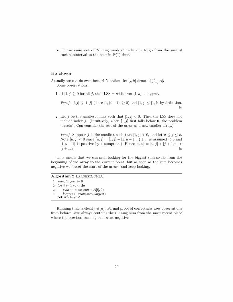
Algorithm 2 LargestSum(A)
1: sum, largest ← 02: for i← 1 to n do3: sum ← max(sum + A[i], 0)4: largest ← max(sum, largest)
return largest
Running time is clearly Θ(n). Formal proof of correctness uses observationsfrom before: sum always contains the running sum from the most recent placewhere the previous running sum went negative.
20

10 (L/P) Graphs (KT 3.1)
Use slides (slides.04.graph-definitions.odp) to present basic defini-tions (undirected, m, n, matrix vs adj list representations, paths, connectivity,cycles, trees).
Theorem 10.1. Let G = (V,E) be a graph with |V | = n ≥ 1. Any two of thefollowing imply the third:
1. G is connected.
2. G is acyclic.
3. G has n− 1 edges.
Do these proofs carefully—as a model for them!
Lemma 10.2. (1, 2) =⇒ (3). If G is acyclic and has n − 1 edges, then G isconnected.
Proof. Suppose we have a graph G which is connected and acyclic, with nvertices. We prove that it has exactly n − 1 edges by induction on n. Proofidea: induction; show we can always find a leaf to delete.
• When n = 1, there are indeed n− 1 = 1− 1 = 0 edges.
• In the inductive case, we assume the lemma holds for all connected, acyclicgraphs with n− 1 vertices.
Pick a vertex v1 ∈ V and take a walk v1, v2, . . . , never repeating an edge.Claim: we must eventually reach a leaf (a vertex with degree 1) in at mostn−1 steps. All the vertices must be distinct since we can never backtrackalong an edge and G has no cycles. So we can take at most n − 1 stepsbefore we have visited all the vertices. Also, we must get stuck at a leafvj : if we get stuck at a vertex with more than one edge that we’ve visited,it would create a cycle; it’s impossible to get stuck at a vertex with degree0 (we could have picked v1 to be such) because G is connected.
Now consider G − vj , that is, (V − vj, E − vj , vj−1). It has n − 1nodes and no cycles (removing an edge can’t create any cycles), and it isalso connected (since we removed a leaf). So by assumption it has n − 2edges; hence G has n− 1.
SDG
Lemma 10.3. (2, 3) =⇒ (1). If G is acyclic and has n − 1 edges, then G isconnected.
21

Proof. Proof idea: counting argument.Suppose G is acyclic and has n− 1 edges. Let l be the number of connected
components of G; we wish to show that l = 1.Number the components of G arbitrarily, and let component j of G have
kj vertices. Then∑l
j=1 kj = n (the sum of all the components gives the totalnumber of vertices). Each connected component is connected and acyclic, soby the previous lemma it has kj − 1 edges. Since every edge of G lies in somecomponent, we can add these up to get the total number of edges in G:
|E| =l∑
j=1
(kj − 1) =
l∑j=1
kj
− l = n− l
But we assumed |E| = n− 1, so in fact l = 1. SDG
Lemma 10.4 (Handshake lemma). In an undirected graph G = (V,E),∑v∈V
deg(v) = 2|E|.
Proof. Each edge gets counted twice, once in the degree for each of its endpoints.SDG
Lemma 10.5. (1, 3) =⇒ (2): If G is connected with n − 1 edges, then it isacyclic.
This one will be on the HW.
22

11 (L) BFS (KT 3.2, 3.3)
As a quick review, recall how we represent graphs as a data structure in aprogram. Typically we want to use a so-called adjacency list structure, wherewe store a dictionary mapping each vertex to information about its adjacentedges. It is called an “adjacency list” since traditionally each vertex might beassociated with a list of adjacent edges. However, it makes much more senseto use a set rather than a list: UGraph = Map<Vertex, Set<Vertex>>. For aweighted graph we can use WGraph = Map<Vertex, Map<Vertex, Weight>>. Ifwe assume Θ(1) lookup for maps or sets (e.g. using a hash table implementation),this lets us look up a particular edge in Θ(1) and iterate over all neighbors of agiven vertex in Θ(deg(v)).
Today we’ll start exploring variants on the s-t connectivity problem, a fun-damental question we can ask about a graph:
1. Given vertices s, t in an undirected graph G, is there a path from s to t?
2. What is the length of the shortest path from s to t?
These problems come up in lots of applications, e.g. the number of introduc-tions needed to connect to someone in a social network; path planning e.g. fora robot in a factory; etc.
This problem is solved by the breadth-first search algorithm. Idea: start atvertex s and explore outward in all directions, adding vertices one “layer” ata time. That is, L0 = s; L1 = all neighbors of L0; . . .Li = all neighbors ofLi−1 not in any previous layer.
23

Properties of BFS:
1. The shortest path from s to v has length i if and only if v ∈ Li. (Theproof is by induction on i: in the base case i = 0 and L0 = s; then, ifwe assume it is true for Lk, we can show it is also true for Lk+1.)
2. There exists a path from s to t if and only if t is in some layer of the BFSfrom s.
3. For each (u, v) ∈ E, the layer of u and v differ by at most 1. (As soon asone shows up the other will show up in the next layer. Note they couldbe in the same layer.)
Thinka of the BFS as making a tree:
We can store the tree simply using a dictionary π (which stands for πarent)mapping each vertex to its parent in the BFS tree. This is good enough sincewe never need to traverse back down the tree. To find a shortest path from sto some ending vertex we just look up the ending vertex in the tree to get itsparent, then look up its grandparent, and so on, until we reach s; the final pathis just the reverse of the vertices we visited on our way up the tree.
BFS, formally:
24

Algorithm 3 BFS(G,s)
Require: Undirected graph G = (V,E), vertex s ∈ V .1: Q← empty queue2: π ← empty dictionary (parent map)3: level ← empty dictionary (level map)4: Mark all vertices Unvisited5: Mark s Visited, add s to Q, level [s]← 06: while Q is not empty do7: remove u from Q8: for each edge (u, v) adjacent to u do9: if v is Unvisited then
10: Mark v Visited11: π[v]← u12: level [v]← level [u] + 113: Add v to Q
return π, level
Notes:
• We could also make a version that takes a target vertex and stops early,returning just a path from s to t.
• Keeping track of the level array is optional.
• Note we can actually tell whether a node has been Visitedby whether ornot it exists as a key in the level map.
Running time? Two nested loops—Θ(V 2)? Not necessarily!
Theorem 11.1. This implementation of BFS runs in Θ(V + E) time (if thegraph uses an adjacency list representation).
Proof. Line 4 takes Θ(V ). Use an array/dictionary of booleans. Or if we usee.g. a hash table-based set, we can initialize an empty set of visited vertices inΘ(1) time.
Note on line 8, assuming G is using an adjacency list, it takes only Θ(deg(u))to iterate over edges adjacent to u. (If adjacency matrix this is not as efficient.)
Loop on line 8 executes a TOTAL of 2|E| times, twice for each edge, becauseeach vertex ends up being visited exactly once. Note we don’t really have toconsider the loop on line 6, since we can directly quantify the TOTAL numberof times the innermost loop executes.
Now, how about the contents of the innermost loop?
• Checking whether Visited or Unvisited takes Θ(1) given array/dictionary.
• Adding edge to π is Θ(1).
• Adding v to Li+1 is Θ(1), just add to end of list or something.
25

Hence total time is Θ(V ) + Θ(E) = Θ(E + V ), or just Θ(E) if we use a setto represent visited vertices. SDG
Of course Θ(E+V ) = Θ(max(E, V )), but we don’t a priori know which oneis bigger. Θ(E) can be as small as Θ(1) (if there are very few edges, i.e. thegraph is sparse) and as big as Θ(V 2) (if there are a lot of edges, i.e. the graphis dense).
26
12 (L/P) Bipartite and directed graphs (KT 3.4,3.5)
Definition 12.1. An undirected graph G = (V,E) is bipartite if V can bepartitioned into two sets L, R such that every edge has one endpoint in L andone in R. (Draw a picture.)
These show up a lot—they are an important special class of graphs. Theycan be used to model relationships between two sets (e.g. matchings). Manyproblems which are difficult for graphs in general become tractable for bipartitegraphs.
Another way to talk about this:
Definition 12.2. A graph is k-colorable if each node can be assigned one of kcolors such that no two vertices connected by an edge have the same color.
Note that 2-colorable is the same thing as bipartite. We will also talk aboutred/blue instead of L/R. (Aside: the notion of k-colorability for k ≥ 3 turnsout to be algorithmically much more difficult to deal with! We will return tothis much later in the semester.)
Do some examples: draw some graphs and ask whether they are bipartite.
Theorem 12.3. G is bipartite iff it has no odd-length cycles.
Proof. (=⇒) All paths must alternate between L and R. Hence every cycle iseven.
(⇐=) Pick an arbitrary vertex s and run a BFS, generating layers L0, L1,L2, . . . . Then pick
L = L0 ∪ L2 ∪ L4 ∪ . . .R = L1 ∪ L3 ∪ L5 ∪ . . .
Claim: every edge (x, y) ∈ E has one endpoint in L and one in R. Bythe single-layer-difference property of BFS, there can’t be any edges betweendifferent layers within L or R. The only possibility we have to worry about isan edge between two vertices in the same layer.
So, suppose (x, y) ∈ E and x, y ∈ Lj ; we will derive a contradiction. Let zbe the least common ancestor of x and y in the BFS tree (draw a picture), andsuppose z has height h above x and y. Then there is a cycle of length 2h + 1,contradiction.
27

SDG
In fact, we can use this as an algorithmic test for bipartiteness: run a BFSfrom any vertex. Then G is bipartite iff there is no edge within some layer. Ifthere is a cross-edge within a layer, we have found an odd cycle; otherwise, wehave found a 2-coloring of the graph.
Another application of BFS: finding strongly connected components.
Definition 12.4. A directed graph is like an undirected graph except the edgesare ordered pairs of vertices, E ⊆ V × V .
Lots of things generalize naturally to directed graphs: instead of paths wehave directed paths. Instead of degree we have indegree and outdegree. In adirected graph “connected” is “weakly connected”. “Strongly connected” meansbetween any two vertices there is a directed path in both directions. BFS extendsnaturally to directed graphs as well: only follow edges in the direction they aresupposed to go.
Lemma 12.5. A directed graph G is strongly connected iff there is some vertexs such that every other vertex in G is mutually reachable with s (that is, foreach v ∈ V there is a directed path from s to v and another directed path fromv to s).
28

Proof. (=⇒) If G is strongly connected we can pick any vertex as s.(⇐=) Let u, v ∈ V and suppose all vertices are mutually reachable with s.
Then we can construct a directed path from u to v by following the path fromu to s and then from s to v; and vice versa. SDG
Definition 12.6. Given a directed graph G, its reverse graph Grev is the graphwith the same vertices and with all edges reversed.
Theorem 12.7. A directed graph G is strongly connected if and only if allvertices are reachable from some vertex s in both G and Grev.
Proof. A vertex v is reachable from s in Grev if and only if s is reachable from vin G. (A directed path from x to y in G turns into a directed path from y to xin Grev.) So this is really just saying the same thing as the previous lemma. SDG
Corollary 12.8. We can decide whether a directed graph G is strongly con-nected in Θ(V + E) time.
Proof. Pick a vertex s, and run a BFS from s in G and then run another BFSfrom s in Grev. Each BFS takes Θ(V + E) time, and computing Grev takesΘ(E) time. SDG
29
13 (L) DAGs and topological ordering (KT 3.6)
Definition 13.1. A directed acyclic graph (DAG) is a directed graph with nodirected cycles.
In general represents precedence/prerequisites. Courses; compilation; pro-duction pipeline; etc.
Definition 13.2. A topological ordering (topological order, topological sort, top-sort) of a directed graph is an ordering of nodes v1, . . . , vn such that for every(vi, vj) ∈ E, we have i < j.
In other words, we can line up the vertices so that edges only point to theright. (Draw a picture.) This corresponds to an order in which classes can betaken, tasks can be done, etc. so prerequisites are always met.
Theorem 13.3. A directed graph G has a topological ordering iff G is a DAG.
Proof. (=⇒) Suppose G has a topological ordering v1, . . . , vn. We must showthat G has no directed cycles. Intuitively, this is because any directed cyclemust have at least one edge pointing backwards. More formally, suppose thereis a cycle C, whose lowest-numbered vertex is vi, with the previous vertex inthe cycle being vj . But then there is an edge vj → vi with i < j, a contradictionsince v1, . . . , vn is a topological ordering. Hence G has no cycles.
(⇐=) Proof by algorithm! SDG
Lemma 13.4. A DAG has a vertex with indegree 0.
Proof. Proof by algorithm. Pick any starting vertex v, and keep following in-coming edges backwards until finding a vertex with no incoming edges. Thisprocess must stop: if not, by the pigeonhole principle, since there are onlyfinitely many vertices, we must eventually visit a vertex twice, but this wouldform a directed cycle, and we assumed the graph is a DAG. SDG
Proof. Now we prove that if G is a DAG, it has a topological ordering. Proofby induction on n / recursive algorithm.
• Base case: if n = 1 there is only one vertex and no edges, so there is atrivial topological ordering.
• If n > 1, find a vertex v with indegree 0 by the previous lemma/algorithm.Note that G−v (delete vertex and any connected edges) is also a DAGsince deleting things cannot create any cycles. Then by the inductionhypothesis, G−v has a topological ordering. Adding v at the beginningthen makes a topological ordering for G since v has no incoming edges.
SDG
30

This is Θ(V 2): searching for an indegree-0 vertex takes Θ(V ) in the worstcase, and we have to do it once for each vertex. But we can do better when thegraph is sparse. The idea is to maintain some extra information that allows usto quickly find a vertex with indegree 0 on each iteration without searching.
Theorem 13.5. A topological sorting algorithm can be implemented in Θ(V +E) time.
Proof. (Assume adjacency list representation.)We need to be able to quickly find the next remaining vertex with indegree
0 (don’t want to re-run a search every time), and also quickly delete a vertex(updating the indegrees of other vertices appropriately).
Maintain:
• Array/dictionary in[v] = number of incoming edges (indegree) of v. Ini-tialize in Θ(V + E) time (just look at each vertex and count number ofincoming edges).
• Queue/stack/whatever Z of vertices with indegree 0. Initialize in Θ(V )after building in: if in[v] = 0 then add v to Z.
At each iteration, dequeue a vertex v from Z in Θ(1). To delete v, decrementin[u] for each edge (v, u), and add u to Z if in[u] becomes zero. This is Θ(1)per edge and only looks at each edge once in total. Hence Θ(V +E) overall. SDG
The resulting algorithm is known as Kahn’s Algorithm, and was first pub-lished by Arthur Kahn in 1962.
Algorithm 4 TopSort(G)
Require: Directed graph G = (V,E).1: T ← empty list2: Z ← empty queue/stack/whatever (with Θ(1) add/remove)3: in ← dictionary mapping all vertices to 04: for each v ∈ V do5: for each u adjacent to v do6: increment in[v]
7: for each v ∈ V do8: if in[v] = 0 then9: add v to Z
10: while Z is not empty do11: v ← Z.dequeue12: append v to T13: for each u adjacent to v do14: decrement in[u]15: if in[u] = 0 then16: add u to Z
31

14 (P/L) Dijkstra’s algorithm
Though we will continue studying graph algorithms, we will now specificallystudy several greedy algorithms. The basic idea of a greedy algorithm is to pickthe locally best thing at each step. For some problems, we can prove that thisleads to a globally best solution.
So far we have considered undirected and directed graphs, but each edgeeither exists or not. We will now consider weighted graphs, where each edge hassome sort of cost.
Definition 14.1. A weighted (directed or undirected) graph is a graph whereeach edge is assigned a weight. We will denote the weight of edge (u, v) by wuv.
The weight or length of a path is just the sum of the weights of its edges.
For now, we will consider weights in R+, that is, nonnegative real numbers;later, we will consider R; in general, one can use any semiring.
Note that we can think of an unweighted graph as a weighted graph whereall edges have weight 1.
Problem 1 (s-t shortest path). Given vertices s, t, find the shortest (weighted,directed) path from s to t.
Note, almost all solutions actually end up solving a more general problem:
Problem 2 (single-source shortest path (SSSP)). Given a vertex s, find theshortest paths from s to every other vertex. Intuitively, you can’t find shortestpath to just t without exploring the rest of the graph.
In an unweighted graph, we would use BFS, but now we need to take edgeweights into account. Intuition: BFS searches outwards one layer at a time,by increasing distance. We’ll do the same thing: search outward by increasingdistance. Imagine turning on a source of water at vertex s, and watching thewater flood the whole graph. Each edge is a (directed) pipe, and the weight ofan edge says how long the water takes to traverse that pipe.
Note that this only makes sense when the edge weights are positive—if watercan “travel back in time” it invalidates this whole scheme; we can’t necessarilyfind the next vertex to be reached by the water with a greedy approach. Ifwe want to find shortest paths when edge weights can be negative, we need adifferent algorithm (which we will study later).
Here’s the basic algorithm, which we can think of as a generalization of BFSto weighted graphs. Recall that BFS keeps track of
• a set of visited vertices,
• a list of layers,
32

• the parent map π.
The list of layers is really telling us the shortest distance to the nodes in eachlayer, since the distance is just the number of edges. The appropriate general-ization will thus keep track of:
• the set S of vertices that the water has reached;
• the shortest distance d[v] from s to d (i.e. how far did the water have togo before it first reached v?),
• the predecessor π[v] of each vertex in the shortest path from s to v (i.e.where did the water come from when it first reached v?) We can use π toreconstruct the shortest path from s to any vertex v (just start at v anduse π to follow edges backwards).
Algorithm 5 BasicDijkstra(G,s)
Require: Weighted graph G = (V,E), vertex s ∈ V .1: S ← s2: d[s]← 0, all other d[v]←∞3: while S 6= V do4: Pick u ∈ S, v /∈ S such that d[u] + wuv is as small as possible.5: π[v]← u6: d[v]← d[u] + wuv
7: Add v to Sreturn π, d
33
How long does this take? It depends a lot on how we implement line 4. Abrute-force approach simply iterates over all edges (u, v), filters out only thosewith u ∈ S and v /∈ S, and picks the one with the smallest d[u] +wuv. Since thewhile loop adds one vertex to S on each iteration, it executes |V | times, makingthe whole algorithm Θ(V E) (which could be O(V 3) if the edges are dense). Itturns out we can do better than this if we use a more clever scheme for quicklyfinding the best edge on line 4.
34

15 Dijkstra proof and asymptotics
Theorem 15.1. Dijkstra’s algorithm correctly solves the SSSP problem for aweighted graph with nonnegative edge weights.
Proof. We will prove the loop invariant that for all v ∈ S, d[v] is the length ofthe shortest path from s to v.
The proof is by induction on the number of loop iterations.
• At the start of the algorithm, S = s and d[s] = 0.
• Now suppose the invariant holds and the loop executes one more time.Let u, v be the vertices picked by the algorithm. We will show that anyother path from s to v must be at least as long as the path from s to vvia u. [Draw a picture.] Any other path from s to v must exit S at somepoint, say the edge where it exits S is x → y. But by the way u, v werechosen, we know that the shortest path from s to y via x is at least as longas the path from s to v (since by the invariant we know the shortest pathfrom s to x), plus there may be extra distance from y to v as well. (Noticehow the assumption of nonnegative edge weights is important here—if thedistance from y to v could be negative it invalidates this proof!)
Hence, the loop updates S and d appropriately and the invariant stillholds.
SDG
How fast can we make Dijkstra run? While loop obviously executes n times.The crux of the issue is how long it takes to pick the best u and v. Brute-force:just consider every edge and find the minimum. Then the whole algorithmwould be Θ(V E) which could be as high as O(V 3). Can we do better?
The key, as usual, is to use some data structures to keep track of enoughinformation so that we can pick u and v quickly without having to search throughthe whole graph every time.
• We will expand d to keep track of not just the shortest distances to verticesin S, but the current shortest known distances to other vertices as well.So d[v] will always be an upper bound on the shortest distance from s tov. We may have to update d[v] every time we add a vertex u to S withan edge (u, v).
• We will expand π similarly: π[v] is the predecessor of v along the currentshortest known path from s.
Idea: at each iteration we want to pick the vertex v /∈ S with the smallestd[v]. We will store the vertices v /∈ S in some kind of data structure so that wecan quickly remove the one with the smallest d[v]. We then need to be able toupdate d and π appropriately.
35

So we need a data structure that supports the following operations, i.e. apriority queue:
Array/dict Sorted array Binary Heap Fibonacci HeapRemove min Θ(n) Θ(1) Θ(lg n) Θ(lg n)Decrease key Θ(1) Θ(n) Θ(lg n) Θ(1)
(Annoying note: Java’s standard library does not have a priority queueimplementation capable of doing a fast decreaseKey operation. One can simplyremove an element and re-insert it, but this takes Θ(n) since there is no way tofind an element other than scanning over the entire heap. An implementationsupporting a fast decreaseKey could, for example, keep a hash table on the sidewhich keeps track of the location of each item within the heap.)
Algorithm 6 Dijkstra(G,s)
Require: Weighted graph G = (V,E), vertex s ∈ V .1: S ← 2: d[s]← 0, all other d[v]←∞3: Create priority queue Q containing all nodes, using d[v] as the key for v.4: while Q is not empty do5: u← Q.removeMin6: Add u to S7: for each outgoing edge (u, v) from u do8: if v /∈ S & d[u] + wuv < d[v] then9: d[v]← d[u] + wuv
10: Q.decreaseKey(v, d[v])11: π[v]← u
return π, d
Time complexity? Again, we can’t just simplistically look at loops and soon. Instead, we count the total time taken by various operations.
• For any reasonable implementation of Q, creating it in the first place takesΘ(V ) time since we are inserting vertices with known keys all at once.
• We end up calling removeMin once for each vertex, and Q has size at most|V |, which contributes Θ(V ·Tremove(V )) (the PQ decreases each time, buthalf the calls are on a priority queue of size at least V/2, so we are stilljustified in saying it takes Θ(V · Tremove(V ))).
• We also call decreaseKey once for each edge, which contributes Θ(E ·Tdecrease(V )).
• All other operations (adding to S, checking for membership in S, settingvalues in d and π) take Θ(1), which adds Θ(V + E) overall.
So in total, the algorithm takes Θ(V · Tremove(V ) + E · Tdecrease(V )). We’llgenerally assume that |E| ≥ |V | (otherwise the graph is either a tree, in which
36

case we don’t need this algorithm, or there are degree-zero vertices which wecan throw away). Total running time depends on implementation of Q:
• Sorted array: Θ(V + EV ) = Θ(EV ).
• Array/dictionary: Θ(V 2 + E) = Θ(V 2) (since E < V 2).
• Binary heap: Θ(V lg V +E lg V ) = Θ(E lg V ) (since we assume |E| ≥ |V |).
• Fibonacci heap: Θ(V lg V + E).
Fibonacci heap is fastest known implementation. But for simplicity of imple-mentation and speed in practice, binary heap is best all-around.
37

16 (L) Minimum Spanning Trees (MSTs)
Input: a weighted, undirected graph G = (V,E) (with weights in R+, i.e.nonnegative).Output: A minimum-weight spanning subgraph: that is, a set of edges T ⊆ Esuch that (V, T ) is connected and T has the smallest total weight among allsuch spanning subgraphs.
Applications: connect things with minimum cost (assuming no redundancyis needed), e.g. transportation or communication networks.
Observation 4. Any minimum-weight spanning subgraph (MWSS) is a tree.
Proof. A MWSS is connected by definition. If a spanning subgraph has a cycle,we can remove any edge from the cycle, resulting in a spanning subgraph that isstill connected but with smaller weight. Hence any MWSS must be acyclic. SDG
A MWSS is thus usually referred to as a minimum spanning tree (MST).Given a graph, how can we compute a MST? Do an example, come up with
greedy algorithms. Draw a second copy (have a student make the copy whiledrawing the first copy) and try a different algorithm.
• Kruskal: repeatedly pick the shortest edge that doesn’t make a cycle.
• Prim: repeatedly pick the shortest edge that expands the growing tree.
• (Reverse-delete: repeatedly delete the biggest edge that doesn’t disconnectthe graph.)
38

Lots of greedy algorithms work! It’s almost like we can’t mess it up. Howto prove this?
Lemma 16.1 (Cut Property). Let X, Y partition V and let e = (x, y) be theshortest edge crossing the (X,Y ) cut (that is, the shortest edge with x ∈ X andy ∈ Y ). Then e must be in any MST.
Proof. Suppose we have a spanning tree T that does not include edge e; we willshow that it is not a MST (and hence every MST must include e). Considerthe unique path in T from x to y. It must cross the cut at least once, say ate′ = (x′, y′). Exchange e for e′: the resulting graph is still connected, since anypath that used to go through e′ can now go through e. The resulting graph alsohas lower total weight, so T was not a minimum spanning tree. SDG
This is an exchange argument, which is a general technique when provingsomething is not minimal—find appropriate things to exchange so the totalweight becomes smaller (while preserving any relevant properties). Note wecan’t exchange e with any edge across the cut! For example. . . We particularlyfound the edge on the path from u to v since that guarantees we can exchangeit with e while preserving connectivity.
Theorem 16.2. Kruskal’s algorithm is correct.
Proof. Suppose at some step the algorithm picks e = (x, y). Take X to bethe set of nodes connected to x so far (not including e); x ∈ X by definition.y /∈ X since e would then make a cycle, and Kruskal wouldn’t have picked it.By definition Kruskal picks the smallest such e. So the chosen edge must be ina MST by the cut property. SDG
The proof for Prim’s algorithm is very similar; left as an exercise.
39
17 (L*) Implementing MST
Let’s implement Prim’s algorithm. We’ll build the tree T . S is the set ofvertices connected by the tree so far.
Algorithm 7 HighLevelPrim(G)
Require: Weighted, undirected, connected graph G = (V,E).1: T ← empty tree2: S ← v (pick arbitrary starting vertex v)3: while |S| < n do4: e← smallest edge with one end in S and one end not in S.5: Add e to T .6: Add v to S.
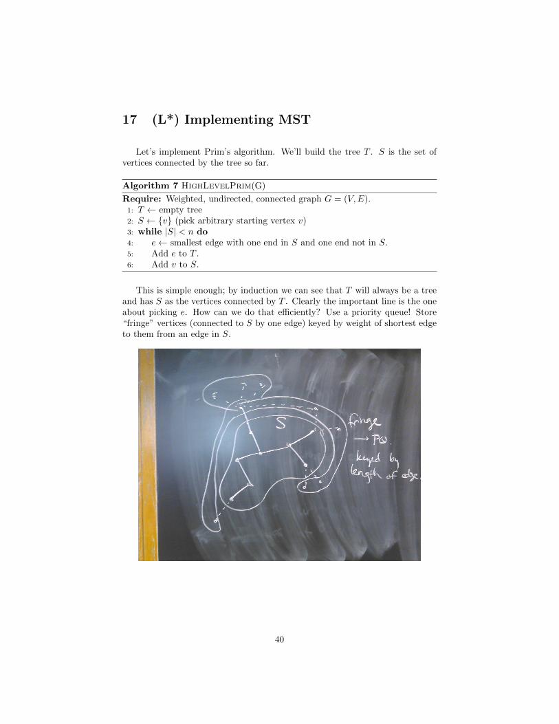
This is simple enough; by induction we can see that T will always be a treeand has S as the vertices connected by T . Clearly the important line is the oneabout picking e. How can we do that efficiently? Use a priority queue! Store“fringe” vertices (connected to S by one edge) keyed by weight of shortest edgeto them from an edge in S.
40

Algorithm 8 Prim(G)
Require: Weighted, undirected, connected graph G = (V,E).1: S ← s (pick arbitrary starting vertex s)2: fringe ← empty priority queue of vertices3: π ← empty parent map4: for each neighbor v of s do5: Add v to fringe using wsv as priority6: π[v]← s
7: while |S| < |V | do8: u← fringe.removeMin9: Add u to S
10: for each edge (u, v) with v /∈ S do11: if v ∈ fringe then12: if wuv < fringe.priority(v) then13: fringe.decreaseKey(v, wuv)14: π[v]← u
15: else16: fringe.add(v, wuv)17: π[v]← u
What’s the running time of this algorithm?
• Lines 1–4 are all constant time.
• The loop at line 5 takes O(V ) time: lines 6 and 7 are constant-timeoperations, and s may have O(V ) neighbors.
• The while loop at line 9 executes |V | times. Line 10 therefore contributesa total of O(V · Tremove(V )) (depending on the priority queue implemen-tation). Lines 11 and 12 are constant so they contribute a total of O(V ).
• Line 16 executes at most once per edge, so it contributes a total of O(E ·Tdecrease(V )).
• Line 20 executes at most once per vertex, so it contributes a total ofO(V · Tadd).
All together, then, this algorithm isO(V+V ·Tremove(V )+E·Tdecrease(V )+V ·Tadd). If we use a binary heap-based priority queue implementation, Tremove(V ) =Tdecrease(V ) = Tadd = Θ(log n), so this becomes O(V + V log V + E log V ) =O(E log V ). If we use a Fibonacci heap, Tremove(V ) = Θ(log n) but Tadd =Tdecrease(V ) = Θ(1), so it becomes O(V +V · log V +E+V ) = O(E+V log V ).These running times are the same as Dijkstra’s algorithm.
41
18 (L) Kruskal’s Algorithm, Union-Find datastructure
Recall Kruskal’s algorithm for computing MST: consider edges in order fromsmallest to biggest, keep each edge unless it would create a cycle with edgesalready chosen. How to implement this?
First idea:
• Initialize T to be an empty graph.
• Sort the edges.
• For each edge (u, v), run a DFS from u in T in and see if we can reach v.If so, adding (u, v) would create a cycle so discard it; otherwise, add (u, v)to T .
How fast is this? Sorting the edges takes Θ(E logE) = Θ(E log V ). (E isO(V 2) so logE is O(log V 2) = O(2 log V ) = O(log V ).) Running a DFS in Ttakes Θ(V +E) = Θ(V ) (since T will never have more edges than vertices), andin this algorithm we run a DFS once for each edge, for a total of Θ(V E), whichdominates the Θ(E log V ) time to sort the edges. Of course, Θ(V E) can be asbig as Θ(V 3) if there are a lot of edges. Can we do better?
Yes, we can! Notice that for each edge (u, v), doing a DFS is sort of overkill,in the sense that it actually tries to find a path from u to v, but we don’t careabout the path, only whether u and v are already connected or not. In thiscase—when we only care about which vertices are connected and not about theactual paths between them—we can test for connectivity much faster.
The basic idea is to come up with some sort of data structure to maintain aset of connected components. Given such a data structure, the algorithm lookssomething like this:
• Start every vertex in its own connected component.
• For each edge, test whether its vertices are in the same component (whichmeans it would form a cycle) or in different components.
• If the endpoints are in different components, add the edge to T , and mergethe two components into one.
This kind of data structure is called a union-find structure, and from thealgorithm above we can see what operations it needs to support:
• MakeSets(n): create a union-find structure containing n singleton sets.
• Find(v): return the name of the set containing v. (“Name” could beanything, typically we will use integers.) To check whether two verticesu and v are in the same connected component, we can test if Find(u) =Find(v).
• Union(x, y): merge the two sets whose names are x and y.
42

This has lots of applications! (See homework.)Given such a data structure, we can implement Kruskal’s algorithm as fol-
lows:
Algorithm 9 Kruskal(G)
Require: Weighted, undirected, connected graph G = (V,E).1: T ← empty set of edges2: Sort the edges of G by weight3: U ←MakeSets(n)4: for each edge e = (u, v) from smallest to biggest do5: if U.Find(u) 6= U.Find(v) then6: Add e to T7: U.Union(u, v)
• Sorting edges by weight takes time Θ(E logE) = Θ(E log V ).
• We do 2|E| Find operations.
• We do at most |V | − 1 Union operations.
Hence, the overall time is O(E log V + TMakeSets + ETFind + V TUnion). Wewould really like for TFind and TUnion to be O(log V ) (or better), which wouldmake the whole thing O(E log V ).
First idea: just keep a dictionary that maps each node to an “id” whichidentifies its set.
• Find is Θ(1). (Assuming Θ(1) dictionary lookup.)
• But to do Union we have to go through and change all the ids of one ofthe sets. This could be O(n). Not good enough!
log n, eh? This should make us think of trees. Idea: forest (multiple trees)of vertices where each points to its parent. (Parents don’t need to know abouttheir children.) We can represent this simply with an array/dictionary whereπ[v] = p means p is the parent of v; by convention, π[v] = v means v is a root.Each tree is a set; the root of the tree will be used as the name of the set. Nodesare given an id “lazily”—might not point directly to its id.
43

• To do Find, just follow pointers up to the root. That is, given v, look upπ[v], then π[π[v]], and so on, until finding a root.
• To do Union(x, y), just merge the trees by setting one to be the parentof the other, that is, π[x] ← y. Note that this only works if x and yare already roots. (For convenience, one might also want to implement aversion of Union which can work on any nodes, by calling Find on eachfirst and then doing the union.)
Clearly Union is Θ(1), hooray! But what about Find? It seems like itmight be O(n) in the worst case, if we end up with an unbalanced tree. But ifwe are clever/careful in how we implement Union, this won’t happen!
• Keep track of the size of each set (i.e. in a separate array/dictionary).
• When doing Union, always make the smaller set a child of the larger (andupdate the size of the larger in Θ(1)).
Theorem 18.1. Find takes Θ(log n) time.
Proof. The distance from any node up to its root is, by definition, the numberof times its set has changed names. But the name of a node’s set only changeswhen it is unioned with a larger set. So each time a set changes names, itssize must at least double. The total size of a set can’t be larger than n; hencethe most time any element can have its set change names, and therefore itsmaximum depth, is O(log n). SDG
44
One can also implement path compression: when doing Find, update everynode along the search path to point directly to the root. This does not makeFind asymptotically slower, and it speeds up subsequent Find calls. One canshow (although the proof is somewhat involved—it would probably take twolectures or so) that Find then takes essentially Θ(lg∗ n) on average, where lg∗ nis iterated logarithm of n, defined as the number of times the lg function mustbe iterated on n before reaching a result of 1 or less. This means that the largestnumber for which lg∗ n = k is n = 22
2...
with k copies of 2 stacked up in a tower
of exponents! So, for example, lg∗ n ≤ 5 for all n ≤ 2222
2
= 2224
= 2216
= 265536,a number with 19729 decimal digits (for comparison, the number of particlesin the entire universe is estimated at around 1080, a number with a measly 81decimal digits). So although in theory lg∗ n is not a constant—it does dependon n, and can get arbitrary large as long as n is big enough—in practice, in ouruniverse, it is essentially a constant (and a rather small constant at that). Thismeans that both Find and Union can be implemented to run in (essentially)constant time!
Note, however, that this does not change the asymptotic running time forKruskal’s algorithm, which is still dominated by the Θ(E log V ) time needed tosort the edges.
45

19 Huffman coding
46
20 (P/L) Divide and Conquer: Master Theorem
Basic idea of divide & conquer:
• Break input into subproblems.
• Solve subproblems recursively.
• Combine subproblem solutions into overall solution.
When it works, this is a beautiful technique and very amenable to analysis:
• Implementation: recursion
• Correctness proof: induction
• Asymptotic analysis: recurrence relations
Classic example: mergesort. Look at call tree of mergesort to see why it isΘ(n log n): the tree has height lg n, and we do Θ(n) work merging at each level.
Integer multiplication
Input: two n-bit integers A, B.Output: A×B.
Note that adding two n-bit numbers takes Θ(n). The naive grade-schoolalgorithm to multiply them takes Θ(n2): multiply A by each bit of B in Θ(1)time (for each bit of B we either get 0 or a shifted copy of A), and then addthe results—there are Θ(n) shifted copies of A to add, and each addition takesΘ(n), for a total of Θ(n2).
Let’s try a divide and conquer approach. Divide each integer into two n/2-bit halves. (Assume n is a power of two—if not, we could always left-padthe numbers with zeros, which only increases the size by at most a factor of2.) For example, if A = 10510 = 011010012 then A1 = 01102 = 610 andA2 = 10012 = 910. Note 6 · 24 + 9 = 105. In general, A = A1 · 2n/2 + A2 andB = B1 · 2n/2 +B2. Multiplying,
AB = (A1B1)2n + (A1B2 +A2B1)2n/2 +A2B2.
So we have broken the original problem (multiplying two n-bit numbers) intofour subproblems of size n/2 (i.e. four n/2-bit multiplications) plus some ex-tra work to combine the results. Note the combining takes Θ(n) time (threeadditions at Θ(n) each, plus two shifts which take constant time). So if T (n)represents the amount of time needed to multiply two n-bit numbers, we havethe recurrence
T (1) = Θ(1)
T (n) = 4T (n/2) + Θ(n)
We can unroll this into a recursion tree to figure out how much total workhappens:
47

• The tree has height log2 n.
• At depth k, there are 4k recursive calls, each on a problem of size n/2k.
• At each recursive call of size n/2k we do Θ(n/2k) work.
• Hence the total amount of work at level k is 4kΘ(n/2k) = 2kΘ(n).
Hence the total amount of work in the whole tree (noting that 2log2 n = n)is
log2 n∑k=0
2kΘ(n) = Θ(n) + 2Θ(n) + 4Θ(n) + · · ·+ nΘ(n)
= (1 + 2 + 4 + · · ·+ n)Θ(n)
= (2n− 1)Θ(n) = Θ(n2).
Argh! This turns out to be no better than our original naive algorithm. BUTit was a good exercise, and gives us insight into more general situations—notto mention this approach can be salvaged by doing something a bit more cleverwhen we split up the problem into subproblems. But first, let’s prove a moregeneral theorem.
Lemma 20.1. alogx b = blogx a.
Lemma 20.2. For some positive constant r and some variable x, let
S = 1 + r + r2 + · · ·+ rx =1− rx+1
1− r.
48

• If r < 1, then S is Θ(1).
• If r = 1, then S is Θ(x).
• If r > 1, then S is Θ(rx).
Theorem 20.3 (Master Theorem). If
T (n) ≤ aT (dn/be) +O(nd)
for positive constants a, b, and d, then
T (n) =
O(nd) a < bd
O(nd log n) a = bd
O(nlogb a) a > bd.
Intuitively, a tells us how fast the number of recursive calls grows; bd tells ushow fast the problems are getting smaller. The ratio of these will end up beingthe common ratio of a geometric sum.
• If a < bd, then the problems get smaller faster than the number of prob-lems increases, and the total amount of work is dominated by the workdone at the very top of the recursion tree.
• If a > bd, then the number of nodes is growing faster than the workdecreases, so the amount of work is dominated by the bottom level of thetree (as in our integer multiplication example).
• If a = bd, then the growth of the number of subproblems is exactly bal-anced by the decrease in the amount of work, so there is exactly the sameamount of work done in total at each level of the recursion tree (namely,O(nd)), and the overall total is hence this amount of work per level timesthe number of levels (as in merge sort).
Proof. We begin by drawing the recursion call tree:
49

• The tree has height logb n.
• A node at level k has size n/bk and does O((n/bk)d) work.
• There are ak nodes at level k, so the total work at level k is
ak ·O(( n
bk
)d)= O(nd)
( abd
)k.
Hence the overall total work is
logb n∑k=0
O(nd)( abd
)k= O(nd)
logb n∑k=0
( abd
)k.
This is O(nd) times a geometric series with ratio a/bd.
• If a < bd then the ratio is < 1 and the sum is a constant; hence the totalwork is O(nd).
• If a = bd then the ratio is 1 and the sum is O(logb n); hence the total workis O(nd log n).
• If a > bd then the ratio is > 1 and the sum is proportional to its finalterm, (a/bd)logb n. In that case the total work is
O
(nd ·
( abd
)logb n)
= O
(nd · alogb n
(blogb n)d
)= O(alogb n) = O(nlogb a).
SDG
50

21 (L*) Applications of divide & conquer, introto FFT
Karatsuba’s algorithm
Now, back to integer multiplication! In 1960 it seemed “obvious” that integermultiplication was Ω(n2); Andrey Kolmogorov (a really huge name in mathe-matics) posed it as a conjecture. Then Anatoly Karatsuba disproved the con-jecture by coming up with a faster algorithm!
Break up A and B into two pieces of size n/2 as before. Now for Karatsuba’sclever insight. Define
P1 = A1B1
P2 = A2B2
P3 = (A1 +A2)(B1 +B2)
Note P3 − P1 − P2 = A1B2 +A2B1. Hence
AB = P12n + (P3 − P1 − P2)2n/2 + P2.
This requires only three multiplications of size n/2! (Along with two additionsof size n/2, four additions or subtractions of size n, and two shifts—more workthan before, but all still Θ(n) in total.)
Hence T (n) = 3T (n/2) + Θ(n), so we can apply the Master Theorem witha = 3, b = 2, and d = 1. 3 > 21 so we are in the third case of the theorem (thework is concentrated at the bottom of the call tree), and we conclude that thisalgorithm is O(nlog2 3) ≈ O(n1.59).
This is not even the fastest known algorithm—the fastest algorithm actuallyused in practice is the Schonhage-Strassen algorithm, which can multiply two n-bit integers in O(n log n log log n). [Q: what does a theoretical computer scientistsay when drowning? A: log log log . . . ]
Matrix multiplication
Recall how matrix multiplication works. Given n×n matrices X and Y , wewant to compute XY where
(XY )ij =∑k
XikYkj .
(Incidentally, this is much more important than it might seem: there are awhole host of linear algebra operations which can be reduced to doing matrixmultiplication; there are lots of algorithms, e.g. graph algorithms (rememberadjacency matrices?) that can be similarly reduced. . . )
How long does this take? Obvious algorithm is Θ(n3): three nested loops(for each of the n2 elements of the output array, we do n multiplications and n
51

additions). So we can say matrix multiplication takes O(n3). Also, it is clearlyΩ(n2) since the output has size n2. But it seems “obvious” that we can’t doany better than n3. . . can we?
In fact, lots of people used to think Θ(n3) was the best possible, until VolkerStrassen made a surprising discovery—a divide-and-conquer algorithm fasterthan the naive Θ(n3)!
The basic idea boils down to a “trick” (similar in spirit to Karatsuba’s algo-rithm) for computing the product of 2× 2 matrices using only 7 multiplicationsinstead of 8.
XY =
[a bc d
] [e fg h
]=
[ae+ bg af + bhce+ dg cf + dh
]Computing the result directly, as above, obviously requires eight multiplications(and four additions).
Now define:
p1 = a(f − h)
p2 = (a+ b)h
p3 = (c+ d)e
p4 = d(g − e)p5 = (a+ d)(e+ h)
p6 = (b− d)(g + h)
p7 = (a− c)(e+ f)
Computing all the pi requires 10 additions and 7 multiplications. Now, as youcan check,
XY =
[p5 + p4 − p2 + p6 p1 + p2
p3 + p4 p1 + p5 − p3 − p7
].
All told, we have now computed XY using 18 additions and 7 multiplications.This is a terrible algorithm for multiplying actual 2×2 matrices! But we can turnit into a recursive divide-and-conquer algorithm for multiplying large matrices.
Assume X, Y are n × n matrices where n is a power of 2. Break each oneinto four n/2× n/2 submatrices (“blocks”). That is,
X =
[A BC D
]Y =
[E FG H
]where A, . . . ,H are n/2×n/2 matrices. It turns out that matrix multiplicationworks the same way on these blocks as it does for actual 2× 2 matrices, that is,
XY =
[AE +BG AF +BHCE +DG CF +DH
](For proof, see any linear algebra textbook, or just think about it a bit.)
If we do the obvious thing here and make 8 recursive calls, note that we haveT (n) = 8T (n/2)+O(n2), so we can apply the Master Theorem with a = 8, b = 2,
52

and d = 2. Since 8 > 22 the algorithm takes O(nlogb a) = O(nlog2 8) = O(n3):this is just the naive algorithm.
But instead, we can use the above method for multiplying 2 × 2 matrices:this results in only seven recursive calls, and a constant number of extra matrixadditions which still take O(n2) overall. So now a = 7, b = 2, and d = 2: westill have 7 > 22 so the algorithm is O(nlog2 7) ≈ O(n2.81).
Although asymptotically faster than “naive” matrix multiplication, Strassen’salgorithm is
• numerically less stable
• only faster for n > 1000 or so, because of the overhead of extra additionsand so on.
But it’s actually used in practice, especially for multiplying very large matriceswhen numerical stability is not an issue (e.g. over finite fields).
Strassen’s breakthrough spurred a lot more research into the problem. Thecurrently best known asymptotic complexity is about O(n2.37), but such algo-rithms are not used in practice because they would only be faster for astronom-ically large matrices.
Introduction to the Fast Fourier Transform
Problem: multiplying two polynomials of degree n,
p(x) = a0 + a1x+ a2x2 + · · ·+ anx
n,
where the ai are complex numbers (really, any field will do).How fast can we multiply two such polynomials?
• Using a simple naive algorithm we can clearly achieve O(n2).
• We can use Karatsuba’s trick to achieve O(nlog2 3).
But it turns out we can do even better, using the Fast Fourier Transform (FFT).The FFT is one of the most important algorithmic developments of the 20thcentury, and has tons of applications in engineering, physics, chemistry, astron-omy, geology, signal processing. . . Particular applications you may be familiarwith include encoding and decoding DVDs, JPEGs, and MP3s, as well as speechprocessing (i.e. every time you speak to your phone or your computer, it prob-ably runs FFT).
Operations on polynomials, represented in the usual way by a list of n + 1coefficients a0, a1, . . . , an:
• Addition: O(n).
• Evaluation: O(n) using Horner’s method : a0+x(a1+x(a2+· · ·+x(an) . . . ))
• Multiplication (convolution): O(n2) brute force.
a0b0 + (a0b1 + a1b0)x+ (a0b2 + a1b1 + a2b0)x2 + . . .
53

Let’s consider a different representation of polynomials, based on the
Theorem 21.1 (Fundamental Theorem of Algebra). Any nonzero degree-npolynomial with complex coefficients has exactly n complex roots.
Corollary 21.2. A degree-n polynomial is uniquely specified by its value at n+1distinct x-coordinates.
Proof. If f and g are two degree-n polynomials which have the same value ateach of n+ 1 distinct x-coordinates, consider the polynomial f − g: it has n+ 1roots but degree ≤ n; the only way for this to happen is if f − g = 0, that is,f = g. SDG
So another way to “represent” a degree-n polynomial is by a list of n + 1pairs (xi, f(xi)), i.e. some choice of n+ 1 distinct x-coordinates along with thevalue of the polynomial at each.
How fast can we do operations given this representation?
• Addition: O(n). Just add corresponding y-values.
• Multiplication: O(n). Just multiply correpsonding y-values! Actually,there is a subtlety here: the resulting polynomial may have degree 2n, sowe need to make sure we have values of the polynomials for at least 2n+1points to start. (No big deal.)
• Evaluation: actually O(n2) using Lagrange’s formula.
The point is that these two representations represent a tradeoff: do we wantmultiplication to be fast, or evaluation?
And this raises a natural question: how fast can we convert between the tworepresentations? If we can convert faster than O(n2) then we win!
a0, a1, . . . , an// (x0, y0) . . . (xn, yn)oo
fast eval fast multiply
This is what FFT does: it can convert in O(n log n). So, for example, to multiplytwo polynomials represented by their coefficients, we can convert to the set-of-points representation in O(n log n), multiply in O(n), and convert back inO(n log n), for a total time of O(n log n). The key will be to cleverly pick thexi we will use as our points at which to evaluate the polynomial.
22 (L*) FFT
Details of FFT; see slides.
54

23 (L) Median/select
Remember the 3 components of divide & conquer:
• Divide input into subproblems somehow (split, partition, . . . )
• Recursively solve the subproblems (have faith they are correct!)
• Combine the answers
Don’t forget base case(s) as well.To prove (by induction on size of input!):
• Prove base case(s) are correct
• Prove: if answers to subproblems are correct, then answer to whole prob-lem is correct.
Array Median
Input: array of n integers.Output: the median element, i.e. the bn/2c-smallest.
In groups: what’s the first algorithm you think of? How long does it take?(Probably sort + return middle, Θ(n lg n).)
Can we do better? Get ideas.Problem: if we e.g. split the array in half somehow and get the median of
both, that wouldn’t really help. The medians of the subarrays are not likely tohave any relationship to the median of the whole.
Solution: generalize! Let’s find not just the median, but take k as an inputand return the kth-smallest. Select(A, k): return the kth-smallest element ofarray A. We can get median by calling Select(A, bn/2c).
Question: how should we split up the array? Just splitting down the middledoesn’t really help. What’s a different way we could split up A (think in groups).Hint: think of other divide & conquer algorithms you know. (Quicksort.)
Solution: pick a pivot element p (random!) and partition into A1 = allelements < p and A2 = all elements ≥ p. Then if k < |A1| return Select(A1, k),else return Select(A2, k − |A1|).
Prove correct. Analyze time complexity.
55

24 (P/L) Intro to dynamic programming
“Dynamic programming”—not really either. Name chosen by Richard Bell-man in 1950 as something that sounded good to government / funding agencies.
Last week we looked at the divide and conquer technique: a problem getsbroken down recursively into subproblems. We’re still considering the samephenomenon—dynamic programming is about what to do when the recursivesubproblems overlap. Basic idea: save answers to recursive subproblems (memo-ization) so we don’t have to compute them more than once. DP has a reputationfor being difficult/confusing, but at heart it’s just this simple idea.
Example: Fibonacci numbers
Recall 0, 1, 1, 2, 3, 5, 8, 13, 21, . . . , each number is the sum of the previous two.
F0 = 0
F1 = 1
Fn = Fn−1 + Fn−2
Obvious recursive algorithm is too slow (in fact, it’s O(ϕn)).
# Fibonacci #1: naive recursive algorithm
def fib1(n):
if n <= 1:
return n
else:
return fib1(n-1) + fib1(n-2)
Why is that? Draw out recursion tree for F5. Notice many redundant callsto subproblems. The core idea of dynamic programming is extremely simple:save the results of recursive subproblems so each only needs to be computedonce. Memoization.
We have two options (show fib.py):
• Create an array to hold Fn values and fill it in from 0 to n using a loop.This is the “standard” DP solution. Pros: Efficient, works well even inlanguages without good support for recursion. Con: we have to manuallyfigure out the correct order to fill in the array, so we have already computedthe answer to subproblems when we need them. Simple in this case, butcan be tricky in general.
# Fibonacci #2: explicitly filling in a table with a loop
def fib2(n):
fibs = [0] * (n+1)
fibs[1] = 1
56

for i in range(2, n+1):
fibs[i] = fibs[i-1] + fibs[i-2]
return fibs[n]
• Keep our recursive function, but every time it is called, check whether theanswer for that input has already been computed and saved. If so, returnit; if not, compute it recursively, save it, and return it. Pros: simple tocode; we don’t have to worry about the right order in which to fill thingsin. Cons: a bit more overhead; can run into recursion limits. (Plug forfunctional programming: lazy, immutable arrays. . . )
# Fibonacci #3: recursion with memoization
# Keep a global table to remember the results of fib3
fibtable = [0,1]
def fib3(n):
# Expand the table as necessary
while len(fibtable) < n+1:
fibtable.append(-1)
# Fill in the table recursively (only if necessary)
if fibtable[n] == -1:
fibtable[n] = fib3(n-1) + fib3(n-2)
return fibtable[n]
Example: Low/High Stress Jobs
Consider the following table composed of n weeks where each week i has lowstress job that pays Li and a high stress job that pays Hi.
WEEK 1 2 3 · · · nlow stress L1 L2 L3 · · · Ln
high stress H1 H2 H3 · · · Hn
Each week you are allowed to pick either a low stress job or a high stress job,however, picking a high stress job at week i means that you must take the weekbefore (i.e. week i− 1) off. Your goal is to maximize total income.
We’ve studied greedy algorithms; definitely the thing to try first. Whatwould a greedy algorithm look like? See Algorithm 13 below.
This algorithm basically looks ahead one week and decides if it’s worth takinga week off in order to land a higher-paying job. However, this strategy fails,because taking a high stress job at week hi means that you cannot take weekhi off to take a job at week hi+1. Thus, any strategy employing look-ahead bya constant factor will fail. Here is a counter-example to the greedy algorithm.
57

Algorithm 10 GreedyJob
1: while i ≤ n do2: if i < n and Hi+1 > Li + Li+1 then3: Take week i off, choose Hi+1 and continue with i← i+ 24: else5: Take Li and continue with i← i+ 1
WEEK 1 2 3Low Stress 2 2 1High Stress 1 5 10
• Greedy: 5 (week 2) + 1 (week 3) = 6
• Optimal: 2 (week 1) + 10 (week 3) = 12
The key to solving this problem is to come up with a recursive solution,and then use dynamic programming. The key idea (common to many similarproblems) is to consider the most we could make if we worked only through weeki and then stopped. That is, define OPT (i) = maximum revenue for workingweeks 1 . . . i. Now, we can come up with a recurrence for OPT :
1. Base cases:
• OPT (0) = 0. We don’t make any money for working 0 weeks.
• OPT (1) = L1. We can’t take the high-stress job the first week. (Ormaybe we can—need to clarify problem parameters!)
2. OPT (i) = maxLi + OPT (i − 1), Hi + OPT (i − 2). First, note that ifwe are going to maximize the profit for the first i weeks, we should alwayswork the final week. Thus, our decision is between working a high-stressor low-stress job. Choosing a low-stress job at week i means we shouldadd Li to the optimal profit for the previous i − 1 weeks and choosing ahigh-stress job at week i means we had to take week i− 1 off so we shouldadd Hi to OPT (i− 2). The optimal choice is to choose the max of thesetwo options.
Notice that OPT naturally forms a 1×(n+1) table where each entry requiresΘ(1) operations to fill in. We can fill in the table from 0 to n. So the wholealgorithm is Θ(n). This is the standard way to analyze the running time of aDP solution.
We can also keep a table JOB(i) that tells us which choice we made at weeki (the low stress job or the high stress job) to recover which weeks we shouldactually work. Start with choice at week n and work backwards through thetable. This technique is also standard. In more generality, typically we will betaking some sort of max or min, but this gives us only the value of the max/minand forgets which choice actually leads to it. We can always make a paralleltable that records the optimal choice. In many cases (when there are exactly
58

two choices) it will be a table of booleans. But we will see other examples whereit is a table of e.g. integers.
Do an example:
WEEK 1 2 3 4 5 6 7 8 9 10Low Stress 2 2 1 7 5 20 3 19 10 13High Stress 1 5 10 100 23 20 5 21 30 30
Show jobs.py:
def work_schedule(low, high):
n = len(low)
opt = [0] * n
take_high_job = [False] * n
# If we’re only working one week, take the low-stress job.
opt[0] = low[0]
take_high_job[0] = False
for i in range(1, n):
# How much could we make taking the low or high stress job?
low_total = low[i] + opt[i-1]
high_total = high[i] + (opt[i-2] if i > 1 else 0)
# The optimal for weeks 1..i is the higher of the two
opt[i] = max(low_total, high_total)
# Record which choice produced the higher total
take_high_job[i] = high_total > low_total
# Finally, produce a work schedule: work backwards from the end
wk = n-1
schedule = []
while wk >= 0:
if take_high_job[wk]:
schedule = [’off’, ’HI’] + schedule
wk -= 2
else:
schedule = [’LO’] + schedule
wk -= 1
return (opt[-1], schedule)
59

25 (L*) Matrix chain multiplication
Suppose we have matrices A and B, where A is p× q and B is q× r. (To beable to multiply them, the q has to match.) How many operations are neededto compute the matrix product AB?
• The result AB will be a p× r matrix, so it has pr entries.
• To compute each entry of AB, we take a row of q entries from A and acolumn of q entries from B and multiply them, then add the results. Sowe do about q multiplications and q additions to compute each element ofAB.
Thus, the total time to compute AB is O(pqr). Note that we can assumep, q, and r are small enough that fancy matrix multiplication algorithms likeStrassen’s algorithm don’t really help.
Matrix multiplication is associative, (AB)C = A(BC), but these may nottake the same time to compute! Let’s try an example. Say
• A is 2× 10,
• B is 10× 3,
• and C is 3× 20.
It takes 10 × 3 × 20 = 600 operations to compute BC, resulting in a 10 × 20matrix. It would then take another 2 × 10 × 20 = 400 to compute A(BC), fora total of 1000. On the other hand, if we associate the product as (AB)C, ittakes 2×10×3 = 60 operations to compute the 2×3 matrix AB, and then onlyanother 2 × 3 × 20 = 120 operations to compute (AB)C, for a total of 180—abig difference!
With just three matrices the situation is simple: we can easily just do thesecomputations, compare, and choose the cheaper order. However, if we have asequence of n matrices we wish to multiply, the situation is more difficult. Forexample, suppose we have six matrices A1 . . . A6 and want to compute theirproduct. We could associate them, for example, as (A1((A2(A3A4))A5))A6, oras A1(A2(A3(A4(A5A6)))), or in fact in any of 42 distinct parenthesizations. Wereally don’t want to check all of them to see which would be the cheapest. Ingeneral, the number of parenthesizations for n matrices is the (n− 1)st Catalannumber
Cn =1
n+ 1
(2n
n
)which for large n is approximately equal to
Cn ∼4n
n3/2√π,
60

so the number of possibilities becomes very large, very fast. The brute forcealgorithm—i.e. checking all parenthesizations to see which is best—is completelyout of the question!
Formally, we have a sequence of n matrices A1, A2, . . . , An, and a sequenceof n+1 positive integers p1, . . . , pn+1 such that matrix Ai has size pi×pi+1. Wewant to compute the parenthesization of the Ai which minimizes the numberof operations needed to compute the product A1 . . . An. (Note that this gen-eralizes readily to any situation where we have a sequence of n things and anassociative binary operation where the cost of the operation varies dependingon the arguments it is applied to.)
Observation: ultimately, there will be some final two matrices that get mul-tiplied to produce the final answer. These have to come from some splitting ofthe sequence of matrices into two subproducts
(A1 . . . Ak)(Ak+1 . . . An).
The total cost to compute the product if we split at index k is then given bythe sum of the optimal cost to compute A1 . . . Ak, the optimal cost to com-pute Ak+1 . . . An, and the cost to do the final matrix multiplication, which willtake p1pk+1pn+1 operations (because (A1 . . . Ak) is a p1 × pk+1 matrix, and(Ak+1 . . . An) is a pk+1 × pn+1 matrix). The best possible cost for the productA1 . . . An will then be the minimum cost over all such splitting points k. Ingeneral, if we use m[i, j] to denote the minimum cost for computing the productAi . . . Aj , with i ≤ j, then we have the recurrence
m[i, i] = 0
m[i, j] = mini≤k<j
(m[i, k] +m[k + 1, j] + pipk+1pj+1)
Note that m[i, i] = 0 since this corresponds to the base case of already havinga single matrix Ai, so we do not need to do any work.
We can store the m[i, j] values in an n × n matrix (actually, we just needthe part above the main diagonal since we assume i ≤ j). Note that each m[i, j]depends on values to its left (m[i, k] where k < j) and below it (m[k + 1, j]where k ≥ i). So we can fill in the matrix by diagonals, beginning by fillingin zeros along the entire main diagonal, then filling in values just above themain diagonal, then the second diagonal above the main diagonal, and so on.Note that the dth diagonal above the main diagonal consists of values of theform m[i, i+ d], which corresponds to subproducts Ai . . . Ai+d of exactly d+ 1matrices. So this seems intuitively sensible: first we compute the optimal wayto multiply any two adjacent matrices; then we compute the optimal way tomultiply any three adjacent matrices; then any four, and so on.
(Alternatively, we could arrange the matrix a bit differently, so that m[i, d]would denote the optimal cost for multiplying Ai . . . Ai+d. Then we wouldsimply fill in the matrix by columns.)
The matrix m has size n × n, and we need to fill in half its entries, givinga total of Θ(n2) entries to fill in. Each entry is computed as a minimum over
61

at most n costs, each of which takes O(1) to compute (just a few lookups,additions, and multiplications). Thus the whole algorithm is O(n3).
Notice this has a similar problem as the high/low-stress jobs example: itgives us the optimal cost but doesn’t tell us what the actual best parenthesiza-tion is. This is a common issue with dynamic programming; the problem is thatwhen we take the minimum over all k for each entry in the matrix m, we forgetwhich k was best, recording only the best cost itself. The solution, therefore,is to maintain another n × n matrix b which records the information that isotherwise being forgotten: b[i, j] records the “best split”, that is, the value of k(where i ≤ k < j) which results in the minimum cost for the product Ai . . . Aj .After filling in the matrices m and b, we can reconstruct the best parenthesiza-tion (which is really just a binary tree) by recursively splitting starting from thetop: we start by looking up b[1, n] = k which tells us where to do the top-levelsplit (A1 . . . Ak)(Ak+1 . . . An). We then recursively look up b[1, k] and b[k+1, n]to find out where to make the next splits, and so on, until there are just singlematrices left at the leaves of the tree.
See MatrixChainFull.java for Java implementation.
62

26 (L) The Floyd-Warshall algorithm
Recall that Dijkstra’s algorithm solves the single-source shortest path problem(i.e. it finds the shortest path from a single start vertex to every other vertex) forweighted, directed graphs, as long as all edge weights are positive. Today we willconsider an algorithm to solve the all-pairs shortest path problem (find shortestpath between all possible pairs of nodes) on directed graphs with arbitrary(possibly negative) weights.
Of course, negative cycles can pose a problem: if there is a directed cyclewhose total weight is negative, then we can keep decreasing the path weightforever by just going around the cycle. In that case “shortest” paths may notbe well-defined. The algorithm we consider will also be able to detect thissituation.
Input: a directed, weighted graph G = (V,E) with vertices numbered 1 . . . n.Output: ultimately, we want an n× n matrix s where s[u, v] records the lengthof the shortest path from u to v, or an indication that the graph has negativecycles. Ideally we also want to be able to recover the actual shortest pathbetween any two vertices u and v.
We want to come up with a recurrence. As is typical, we add anotherparameter which we use to restrict the problem. In this case let’s add anotherparameter k that means we are only allowed to use vertices 1 . . . k. That is, lets[u, v, k] denote the length of the shortest path from u to v using only vertices1 . . . k as intermediate nodes on the path.
Base cases?
s[u, v, 0] =
0 u = v
wuv (u, v) ∈ E∞ otherwise
(Note we can’t say s[u, v, k] = 0 for k ≥ 0 because of negative edges!)Now, what about the recursive case? Suppose we already know s[u, v, k] for
some k. Then how can we compute s[u, v, k + 1]? There are two possibilities:either the best path from u to v goes through k + 1, or it doesn’t.
• It could be that allowing vertex k + 1 does not help, in which case
s[u, v, k + 1] = s[u, v, k].
• If it does help, the best path from u to v will consist of first taking thebest path from u to k+1 (using only vertices 1 . . . k), followed by the bestpath from k + 1 to v:
s[u, v, k + 1] = s[u, k + 1, k] + s[k + 1, v, k].
The optimal cost will simply be the minimum of these two.To be able to reconstruct paths after the fact, we could do something similar
to what we usually do: at each step we take a minimum over two choices, so we
63

could keep a parallel 3D table use[u, v, k] that records whether we should usevertex k when trying to go from u to v using only vertices 1 . . . k. We couldthen use this to reconstruct the optimal path from u to v as follows:
bestpath(u, v, k) =
bestpath(u, k, k − 1) + [k] + bestpath(k, v, k − 1)
bestpath(u, v, k − 1)
depending on whether use[u, v, k] is true (with some appropriate base cases aswell).
However, for this problem it turns out we can do something a bit more cleverusing only a 2D array. In particular, let next [u, v] denote the next vertex afteru in the shortest path from u to v that we have found so far. Then in the firstcase, when we set s[u, v, k + 1] to s[u, v, k], we do not change next [u, v]; in theother case, we can update it as
next [u, v] = next [u, k + 1].
Also, we don’t actually need to keep a 3D array for s. We can simply keepoverwriting the same 2D array on each iteration of the loop. If we do that, itis no longer true that s[u, v] is exactly the shortest distance using only vertices1 . . . k on the kth iteration—but if not it can only be shorter.
Algorithm 11 Floyd-Warshall
1: s[u, v]←
0 u = v
wuv (u, v) ∈ E∞ otherwise
2: next [u, v]← v for (u, v) ∈ E3: for u← 1 . . . n, v ← 1 . . . n, k ← 1 . . . n do4: if s[u, k] <∞∧ s[k, v] <∞∧ s[u, k] + s[k, v] < s[u, v] then5: s[u, v]← s[u, k] + s[k, v]6: next [u, v]← next [u, k]
After the algorithm is finished, to reconstruct the shortest path from u to v,we simply look up each step along the path using the next matrix. First we lookup next [u, v] = u2, then we look up next [u2, v] = u3, and so on, until reachingv.
What is the running time? It’s obviously Θ(V 3)—just three nested loopsfrom 1 . . . n. (Which seems kind of amazing given that there could be Θ(V 2)edges and we need to find shortest paths between every pair of vertices, of whichthere are also Θ(V 2).)
What about negative cycles? Well, just look at s[u, u, n]: u is part of anegative cycle if and only if s[u, u, n] (the length of the shortest path from uback to itself) is negative. Hence we can check whether there are any negativecycles in the graph in Θ(n) time, by scanning along the diagonal of the matrixand looking for any negative numbers.
64

As a fun aside, this algorithm is really cool because it can actually be gen-eralized to work over any semiring instead of just (min,+) (technically, anystar-semiring), and it turns out that by appropriate choice of semiring, (a slightgeneralization of) the same algorithm can be used to do a great many things,such as find most reliable paths or largest capacity paths, count the number ofshortest paths or total number of paths or even compute regular expressions forall possible shortest paths, compute transitive closures, invert matrices, solvelinear systems of equations, or convert a DFA into a regular expression.
65
27 (P/L) Amortized analysis: intro
Consider the following problem.
Input: an array B[0 . . . ] representing a binary number n. (Each B[i] is a singlebit representing the coefficient of 2i. Assume B is sufficiently large so we don’thave to worry about problems with overflow.)Output: Increment the binary number, that is, modify B so that it representsthe number n+ 1.
Here is an algorithm to accomplish this:
Algorithm 12 Binary Increment
1: i← 02: while B[i] = 1 do3: B[i]← 04: i← i+ 1
5: B[i]← 1
How long does this take?
• The best case is Θ(1): if the last bit of n is 0 then all we have to do is flipit. The while loop never executes at all.
• The worst case is when n is of the form 2k − 1, that is, all 1 bits, andto increment it we have to flip all the 1’s to 0s and then set the next 0bit to 1. Since n requires Θ(lgn) bits to represent it, this means thatincrementing n takes Θ(lg n) in the worst case.
In practice, we rarely just increment a binary number a single time. Morerealistically, we will be repeatedly incrementing it (perhaps it is a counter ofsome sort). So how long does it take to start at 0, and increment n times?
• We can definitely say it is O(n lg n): we do n increment operations andeach increment takes O(lg n) in the worst case.
• We can also definitely say it is Ω(n): we do n increment operations andeach takes at least Θ(1).
This is a common situation: we have some operation that we want to dorepeatedly, and the operation does not always take the same amount of time.We can easily give an upper bound and a lower bound, but we want to be ableto say something more precise about how long the entire sequence of operationswill take. For this we turn to amortized analysis. The idea of “amortization”is to spread out big one-time costs more evenly (e.g. repaying a car loan or amortgage in monthly installments).
66

n 0 1 2 3 4 5 6 7 8 9 10 11 12 13 14 15 16bit flips 1 2 1 3 1 2 1 4 1 2 1 3 1 2 1 5
cumulative cost 0 1 3 4 7 8 10 11 15 16 18 19 22 23 25 26 31
Table 1: Cost of repeated increments
The first step is almost always to just try small examples, play around,make a table, and notice patterns to come up with a guess. Let’s try it forincrementing a binary counter. We’ll make a table with the counter value n andthe cumulative number of bit flips on the right-hand side. Remember we don’tneed a formula for the number of bit flips2; we are just trying to figure out howfast it grows in relation to n.
We notice some patterns: whenever n is a power of two, the total number ofbit flips seems to be one less than the next power of two. In fact, in general itseems that the cumulative number of bit flips is never more than 2n. Based onthis evidence, we conjecture that a sequence of n increment operations startingfrom 0 actually takes Θ(n), the lower bound we derived from the best case,rather than the worst-case upper bound of Θ(n lg n). Intuitively, it seems likethe “expensive” increment operations happen infrequently enough that theydon’t add too much to the total—we can “average out” their cost over thewhole sequence. In this case we say that a single increment operation takesΘ(1) amortized time: each increment takes Θ(1) “on average”, even though anindividual increment operation could take longer.
So how can we prove this?
Accounting method
Imagine that each constant-time operation “costs” $1. The idea is to overchargefor some operations and “save up” the extra money, so that we have enoughsaved up to pay for expensive operations. In general, if we charge c·f(n) for someoperations and always have enough left over to pay for the other operations, thenwe can say that each operation takes O(f(n)) amortized time.
In this example, we imagine that flipping a bit costs $1. Let’s charge $2every time we flip a bit from 0 to 1. $1 will pay for the flip itself, and the other$1 we imagine being saved next to the 1 bit. Later, when we need to flip the bitback to 0, we will have $1 sitting there which we can use to pay for the flip.
000$2−→ 001
$
$2−→ 01$0
$2−→ 01$1$
$2−→ 1$00
Notice how every increment operation does exactly one 0→ 1 flip, for which wepay $2. And it might do a bunch of 1 → 0 flips, but we get to do those “forfree” using the money we saved up from previous increments. All in all, if wepay $2 for each increment we always have enough money to pay for all the bit
2Though it turns out in this case it is possible to come up with one!
67

flips (without ever going negative). Therefore, we conclude that the amortizedcost of a single increment operation is $2, that is, Θ(1).
As a fun aside, this analysis actually shows us how to come up with a preciseformula for the total number of bit flips needed to increment from 0 to n: afterdoing n increment operations, we have paid $2n, but not all of that $2n hasactually been used. There is $1 sitting next to each 1 bit, and the rest of the$2n has been used to pay for bit flips. So the total number of bit flips neededto increment from 0 to n is exactly
2n−#n
where #n is the number of 1 bits in the binary representation of n.
68

n 0 1 2 3 4 5 6 7 8 9 10 11 12 13 14 15 16incr cost 0 1 3 1 7 1 3 1 15 1 3 1 7 1 3 1 31total cost 0 1 4 5 12 13 16 17 32 33 36 37 44 45 48 49 80
Table 2: Incrementing a counter when flipping bit i costs 2i
28 (L) Amortized analysis II
Direct counting method
Here’s another way we can prove that incrementing a binary counter takes Θ(1)amortized time. AKA “just do some math”. Let’s add up the total number ofbit flips and see what we get. Notice that when doing a sequence of increments,B[0] flips every single time (either 1 to 0 or 0 to 1). Then B[1] flips every othertime, B[2] flips every fourth time, . . . in general B[i] flips every 2ith time. Sowhen incrementing from 0 to n, bit B[i] flips a total of bn/2ic times. Thus, thetotal number of bit flips is
blgnc∑i=0
⌊ n2i
⌋<
∞∑i=0
n
2i= n
∞∑i=0
1
2i= 2n.
This is a sort of “brute force” method of proof which is straightforward whenyou can get it to work. But sometimes it’s easier to use the accounting method.
Another binary counter example
Take the same binary counter incrementing example, but now suppose it costs2i to flip bit i. The worst case for a single increment operation is now Θ(n),since if we have to flip all the bits it will cost 20 + 21 + 22 + . . . which isapproximately equal to n. But once again, the total time to do n successiveincrement operations is actually less than Θ(n2). Let’s again make a table(Table 2) and look for patterns.
Looking at just the powers of 2 might reveal a useful pattern: 2→ 4, 4→ 12,8→ 32, 16→ 80. It looks like each power of 2 is being multiplied by successiveintegers (2×2, 4×3, 8×4, 16×5. . . in particular 2k is being multiplied by k+1.So we conjecture that the total cost to increment from 0 to n is no greater thann × (lg n + 1), which would mean that the amortized cost of each incrementoperation is Θ(lg n).
We could also use the accounting method: every time we do an increment,just put $1 on every bit, whether we flip it or not. (We have to decide up fronthow many bits we are going to use.) Since bit i is flipped every 2i increment op-erations, by the time we flip it we will have accumulated exactly enough moneyto pay for its cost of 2i. Therefore, the amortized cost of a single increment isthe amount we actually pay: we pay $1 for each bit and there are Θ(lg n) bits.
69
[We could also use a direct counting method. Note that bit i is flipped onlyonce every 2i increments, and flipping it costs 2i. So each bit contributes a totalcost that is at most the total number of increment operations. There are lg n+1bits, and each contributes a cost of at most n, for a total of at most n(lg n+ 1).]
Extensible arrays
Another example that should be familiar from Data Structures: extensible ar-rays (e.g. ArrayList in Java). As our cost model, suppose accessing or modify-ing an array entry costs 1, and allocating a new array and copying the contentsof an old array into it costs n (the length of the old array). Every time we doan append operation, it might cost Θ(1) (if there is still enough space in theunderlying array) or it might cost Θ(n) if we have to allocate a bigger array,copy all the elements over from the old array, and then insert the new element.So we can definitely say that a sequence of n append operations is Ω(n) andO(n2).
The question is, what strategy should we use for allocating a new array whenwe run out of space? This turns out to have a big impact on the amortized timeof append.
• Strategy 1: increase the size by some constant c. That is, when our arrayof size n becomes full, allocate a new array of size n + c and copy thecontents of the old array into it.
• Strategy 2: double the size. That is, when our array of size n becomesfull, allocate a new array of size 2n.
Let’s consider the amortized time for a single append operation using thesestrategies.
• Strategy 1: suppose we start with an array of size c. (The starting size ofthe array does not really change the analysis at all.) The first c appendoperations will cost 1 each, and then the next will cost c + 1 (c to copythe now-full array of size c, and 1 more to insert the new element). Thenthere will be another c− 1 operations that cost 1 each until the new arrayis full. The next will cost 2c + 1 (copy the full array of size 2c plus 1 toinsert). And so on.
In general, if we do n successive append operations, we will end up payingn for the actual inserts, plus
c+ 2c+ 3c+ 4c+ · · ·+ bn/ccc
for array allocations. This is
c(1 + 2 + 3 + · · ·+ bn/cc) = c ·Θ((n/c)2) = Θ(n2).
So the total cost for n successive append operations is Θ(n) + Θ(n2) =Θ(n2), and a single append has an amortized cost of Θ(n). In this case,the cost of the expensive operations ends up dominating, even thoughmost of the calls to append are just Θ(1).
70

• Strategy 2: suppose we start with an array of size 1. If we do a sequence ofn append operations, of course we will still pay n for the actual insertions;the question is how much we pay for array allocations. After the initialarray becomes full (immediately), we pay 1 to allocate a new array of size2 and copy the element over. When that becomes full, we pay 2 to allocatean array of size 4 and copy over the old elements. And so on. In total, wewill pay
1 + 2 + 4 + 8 + · · ·+ 2k,
where 2k is the biggest power of 2 which is less than n. But this sum is2k+1 − 1 which is approximately 2n, that is, Θ(n). So the total cost of ncalls to append is Θ(n) + Θ(n) = Θ(n), and the amortized cost of a singleappend is only Θ(1).
We can also prove this using the accounting method. Charge $3 for eachappend. $1 goes to paying for the actual array insertion; the other $2 issaved along with the inserted element. Each time the array becomes full,it will look something like this:
1 3 19 −5 6$$
8$$
21$$
0$$
Since the array capacity was doubled the last time it was resized, for eachelement already in the array there will be a newly inserted element with$2 stored next to it. Therefore the total amount of money available isequal to the number of elements in the array, and we can pay to allocatea new array and copy all the elements over.
Thus, the amortized cost of a single append operation is $3, that is, Θ(1).
71

k 1 2 3 4 5 6 7 8 9 10 11 12 13 14 15 16incr cost 1 1 1 4 1 1 1 1 9 1 1 1 1 1 1 16total cost 1 2 3 7 8 9 10 11 20 21 22 23 24 25 26 42
Table 3: Table of costs with f(k) = k when k is square, 1 otherwise
29 (P*) More amortized analysis examples
Let’s consider another example. Suppose we are doing some sequence of opera-tions where the kth operation takes f(k) = k time when k is a perfect square,and f(k) = 1 otherwise. We can make a table and look for patterns (Table 3).No obvious pattern jumps out at us. So let’s try a more direct approach. Sup-pose we add up all the costs from 1 up to some n = m2:
total = 1 + 1 + 1 + 4 + 1 + 1 + 1 + 1 + 9 + · · ·+m2
We can separate out all the 1’s and the squares:
(1 + · · ·+ 1) + (1 + 4 + 9 + · · ·+m2)
We know there are exactly m2−m copies of 1 (though it actually doesn’t matterall that much: we want an upper bound so it would be enough to say the sumof all the 1’s is less than m2). So the sum is
(m2 −m) +
m∑j=1
j2.
We can look up a formula for the sum of squares, and find this is equal to
m2 −m+m(m+ 1)(2m+ 1)
6.
We could do a bunch of algebra at this point, but we don’t need to: all we careabout is that this is clearly Θ(m3). Note, however, that n = m2, so the sum isΘ(n3/2). Hence the amortized time for a single operation is Θ(
√n).
We said earlier that no pattern jumped out at us from the table—but reallythat’s just because we didn’t try hard enough. We are computer scientists, wedon’t have to just stare at things with our eyeballs! Make a spreadsheet, orwrite a program to generate a bunch of data points, and fit a curve to it. Thisgives us a good guess to start from.
72
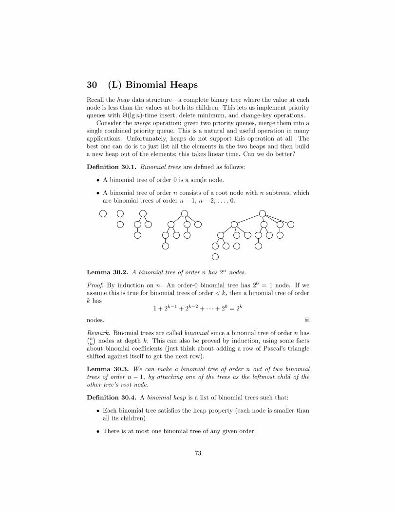
30 (L) Binomial Heaps
Recall the heap data structure—a complete binary tree where the value at eachnode is less than the values at both its children. This lets us implement priorityqueues with Θ(lg n)-time insert, delete minimum, and change-key operations.
Consider the merge operation: given two priority queues, merge them into asingle combined priority queue. This is a natural and useful operation in manyapplications. Unfortunately, heaps do not support this operation at all. Thebest one can do is to just list all the elements in the two heaps and then builda new heap out of the elements; this takes linear time. Can we do better?
Definition 30.1. Binomial trees are defined as follows:
• A binomial tree of order 0 is a single node.
• A binomial tree of order n consists of a root node with n subtrees, whichare binomial trees of order n− 1, n− 2, . . . , 0.
Lemma 30.2. A binomial tree of order n has 2n nodes.
Proof. By induction on n. An order-0 binomial tree has 20 = 1 node. If weassume this is true for binomial trees of order < k, then a binomial tree of orderk has
1 + 2k−1 + 2k−2 + · · ·+ 20 = 2k
nodes. SDG
Remark. Binomial trees are called binomial since a binomial tree of order n has(nk
)nodes at depth k. This can also be proved by induction, using some facts
about binomial coefficients (just think about adding a row of Pascal’s triangleshifted against itself to get the next row).
Lemma 30.3. We can make a binomial tree of order n out of two binomialtrees of order n − 1, by attaching one of the trees as the leftmost child of theother tree’s root node.
Definition 30.4. A binomial heap is a list of binomial trees such that:
• Each binomial tree satisfies the heap property (each node is smaller thanall its children)
• There is at most one binomial tree of any given order.
73

8
21
99
17
5
77
28
13
24
53
33
23
12
We usually keep the list of binomial trees sorted from smallest to biggestorder, stored using a linked list. (I will draw them sorted from right to left.)Notice that a binomial heap acts a lot like a binary number: since binomialtrees have sizes that are powers of two, and a binomial heap has at most onetree of any given order, it is not hard to see that a binomial heap with n totalelements has a binomial tree of order k if and only if the 2k bit of the binaryrepresentation of n is a 1. For example, the heap illustrated above has 13 nodes,132 = 1101, and indeed the heap has one tree of order 1, one of order 4, andone of order 8. This also means a binomial heap of size n contains O(lg n) trees,from order 0 up through order blg nc.
To merge two binomial trees of the same order, just see which one has thebigger root, and make it the leftmost child of the smaller root. This takes Θ(1)time.
To merge two binomial heaps A and B, we can do what amounts to additionof binary numbers. Iterate through them in parallel. For each order k we havepossibly a binomial tree of order k from A, possibly a tree of order k from B,and we also may possibly have a carry tree of order k, just like we can carry a1 bit when adding binary numbers. (When we start out at k = 0 we have nocarry tree.)
• If there are no trees of order k, the output has no trees of order k. (0+0 =0.)
• If there is only one tree of order k, just copy it to the output. (0 + 1 = 1.)
• If there are two trees of order k, merge them into a single tree of orderk + 1 and make it the carry tree for the next iteration; the output has notrees of order k. (1 + 1 = 10, so output 0 and carry the 1.)
• If there are three trees of order k, copy one of them to the output, andmerge the other two into an order-(k + 1) carry tree. (1 + 1 + 1 = 11:output 1 and carry 1.)
Each iteration of the above algorithm takes constant time: we may have tomerge two trees but that takes constant time. So merging two binomial heapsof size n can be done in Θ(lg n) time, since we do Θ(1) work for each order from0 up to blg nc.
Now, let’s see how we can implement the other priority queue methods aswell:
74

• Insert: to insert a new element x into a binomial heap H, make x into asize-1 binomial heap (containing a single order-0 binomial tree) and thenmerge it with H. This is just like incrementing a binary counter! Soalthough it is O(lg n) in the worst case, it takes Θ(1) amortized time.(This is even better than a standard binary-tree based heap, which alwaystakes Θ(lg n) to insert!)
• Delete-min: iterate through the roots of all the trees to find the smallestin Θ(lg n) time (the smallest element in the entire heap is guaranteed to beone of the roots). Removing it leaves its children, which are binomial treesof order k − 1, k − 2, . . . , 0: a binomial heap! Just merge this remainingbinomial heap with the rest of the heap in Θ(lg n) time. So overall delete-min takes Θ(lg n). (Note we can also keep track of the minimum root sothat finding the minimum can be Θ(1), even though removing it still takesΘ(lg n).)
• Change-key: just bubble the key up or down within its binomial treeuntil it is at the right spot. This takes O(lg n).
31 (L*) Potential method and splay trees
There is one more method we can use to prove amortized time bounds, calledthe potential method, which comes from an analogy with physics. The idea is tothink of a data structure as having some “potential energy”. Operations on thedata structure will sometimes increase the potential energy (storing up someextra energy that can be used later) and sometimes decrease it (releasing someof the stored energy). The amortized cost of an operation is the actual cost ofthe operation plus the change in energy. The change in energy can be positive(in which case the amortized cost is more than the actual cost, and some energyis stored for later) or negative (in which case the amortized cost is less than theactual cost, using up some of the stored energy to pay for the difference).
Consider a sequence of operations on a data structure, and let Di denote thestate of the data structure after the ith operation, and Φi the potential energyof Di. Then the amortized cost of the ith operation (which turned Di−1 intoDi) is defined as
ai = ci + Φi − Φi−1
where ci is the actual cost of the operation. Therefore the amortized cost of thesequence of operations is
n∑i=1
ai =
n∑i=1
(ci + Φi − Φi−1) =
(n∑
i=1
ci
)+ Φn − Φ0.
We need the total amortized cost to be an upper bound on the actual cost,and we can see this will happen as long as Φn − Φ0 ≥ 0, which motivates thefollowing definition:
75
Definition 31.1. Φ is valid if Φi − Φ0 ≥ 0 for all i.
If a potential energy function Φ is valid, it means that the total amortizedcost will always be at least the total actual costs, that is,
n∑i=1
ai ≥n∑
i=1
ci.
So the general technique is to define a potential energy function Φ which startsout as 0 on the initial data structure, and always remains nonnegative. Givensuch a valid potential function, the amortized cost of an operation (defined asthe actual cost plus the change in potential energy) gives a valid bound on theaverage cost of a single operation.
Note that this can be seen as a generalization of the accounting method:the amount of “extra money” stored in a data structure can be thought of as“potential energy”. But the potential method makes it more clear that theenergy does not have to be an integer, nor does it have to be “stored” anywherein particular. In some cases this leads to an easier analysis even though in theorywe could do the analysis using the accounting method (with weird fractionalamounts of money stored in a “bank account”).
Splay trees
As a fascinating application of the potential method we will study splay trees, asort of “self-balancing” variant of binary search trees. Recall that binary searchtrees give us Θ(lg n) insert, lookup, and delete for ordered data, as long as thetrees remain balanced. But if the tree becomes unbalanced these turn into O(n)instead. In some applications it does not matter; if a binary search tree is builtrandomly it is very likely to be balanced. However, in many applications thedata may have characteristics that lead to an unbalanced tree (for example,the data may be already sorted or close to sorted, in which case inserting itsequentially into a naive BST creates an unbalanced tree). There are variousways to solve this problem. What most people think of are sophisticated BSTvariants, such as red-black trees and AVL trees, which work by storing extrainformation in the trees and then using this extra information to make sure thetrees remain balanced. Practically speaking, these are some of the best BSTimplementations, but they are complex, and require reimplementing all the BSTmethods to ensure that the extra information is kept up-to-date and that thetree is rebalanced as necessary.
Splay trees are an intriguing alternative: a splay tree is just a normal binarysearch tree, with no extra information stored anywhere. The twist is that weimplement an extra splay operation which works to make the tree a little morebalanced, and we use this operation in conjunction with other operations suchas lookup and insert, in such a way that the tree tends to stay balanced.
In particular, the Splay operation works by bringing a particular elementto the root of the BST (while keeping all the same elements in the tree and
76

preserving the BST properties). It uses a particular algorithm that we willexplore shortly. However, given such an operation that brings a chosen node tothe root of a BST, let’s see how we update the other BST operations to use it:
• Insert: Whenever we insert a new value into the splay tree (which worksjust like normal BST insertion), we then splay the newly inserted elementto the root.
• Lookup: Similarly, lookup works just like in a normal BST; but afterdoing a lookup we splay the looked up element (or the closest element, inthe case that the element being searched for is not in the tree).
• Join: If all the elements in T1 are less than all the elements in T2, we canjoin them into a single BST by first splaying the largest element in T1 tothe root, then adding T2 as its right child (if the largest element is at theroot of a BST, by definition it has no right child, so there is a clear spaceto add T2).
• Split: To split a BST into two BSTs which contain all the elements lessand greater than a particular target element, respectively, splay the targetelement to the root and then return its two children.
• Delete: Splay the item to be deleted to the root, then join the twosubtrees. (This is only a minor point, but notice how much nicer this isthan the usual BST delete implementation!)
Let’s see how Splay actually works. We find the element x in the treeand then keep moving it up the tree until it reaches the root, according to thefollowing three rules. In general we will use p to denote the parent of x and gto denote its grandparent.
• ZIG. If x is the child of the root of the whole tree, then just do onerotation to move it to the root.
CB
p
A
x
C
BA
x
p
A, B, and C denote arbitrary subtrees. We don’t do anything to themat all, so the rotation takes constant time; we just need to update a fewreferences. In the diagram, x is the left child of the root, so we rotateright, but there is also a second entirely symmetric case when x is theright child of the root and we rotate left.
Note how doing a rotation moves x up while preserving the binary searchtree properties: all the elements in the subtree A are still to the left ofx; all the ements in B remain in between x and p; and C remains to theright of p.
77

• ZIG-ZIG. If x and p are either both left children or both right children,then do two successive rotations: first rotate around g → p then aroundp→ x.
DC
g
B
p
A
x
DC
g
BA
x
p
D
C
BA
x
p
g
Some things to note:
– This rule applies anywhere in the tree, unlike ZIG which only applieswhen x is at a depth of 1. After applying ZIG-ZIG, x has movedtwo levels closer to the root.
– Like ZIG, this takes constant time, since we just do two rotations.
– Again, in the picture x and p are illustrated as both being left chil-dren, but there is an analogous symmetric case when x and p areboth right children.
• ZIG-ZAG. If p is a left child and x a right child, or vice versa, first rotatearound p→ x and then around g → x.
DC
g
BA
p
x
D
C
BA
p
x
g
D
CB
x
A
p
g
32 (L*) Analysis of splay trees
Let’s start with some interactive examples to see how splay trees work in prac-tice, and to gain some intuition for what we are trying to prove. For example,if we start with the tree on the left below, the next tree shows what we get ifwe splay 5 to the root; the tree after that shows what we would get if insteadsplay 4 to the root (starting from the tree on the left again); and so on. Youcan see that as we splay an element from deep in the tree, the other elementstend to “clump up” in twos due to the way we iterate the ZIG-ZIG rule.
6
4
2
1
3
5
0
5
3
2
4
60
1
6
4
3
5
0
1
2
5
4
6
0
1
2
3
6
5
0
1
2
3
4
6
0
1
2
3
4
5
0
1
2
3
4
5
6
78
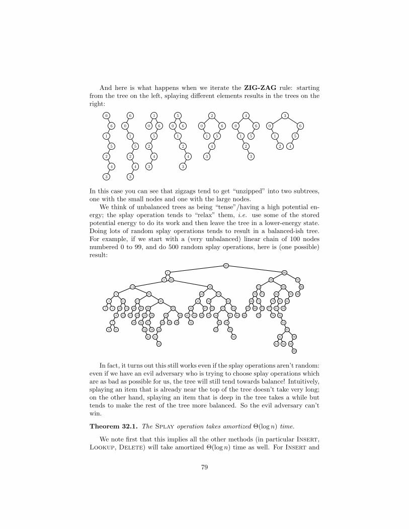
And here is what happens when we iterate the ZIG-ZAG rule: startingfrom the tree on the left, splaying different elements results in the trees on theright:
4
5
6
2
1
0
3
5
6
3
2
1
0
4
3
4
5
6
1
0
2
6
3
4
2
1
0
5
3
4
2
5
60
1
3
4
2
5
1
0
6
3
4
2
5
1
6
0
In this case you can see that zigzags tend to get “unzipped” into two subtrees,one with the small nodes and one with the large nodes.
We think of unbalanced trees as being “tense”/having a high potential en-ergy; the splay operation tends to “relax” them, i.e. use some of the storedpotential energy to do its work and then leave the tree in a lower-energy state.Doing lots of random splay operations tends to result in a balanced-ish tree.For example, if we start with a (very unbalanced) linear chain of 100 nodesnumbered 0 to 99, and do 500 random splay operations, here is (one possible)result:
98
99
97
93
94
95
89
88
90
8684
85
87
83
82
81
91
78
77
79
80
92
75
72
73
71
69
66
67
68
70
74
76
96
64
63
60
59
58
61
55
56
54
57
62
51
52
50
53
46
47
44
42
41
43
45
48
49
38
39
36
32
31
33
34
35
37
28
27
29
24
23
22
25
26
30
18
19
20
15
16
17
21
12
13
86
7
9
10
11
42
3
5
14
400
1
65
In fact, it turns out this still works even if the splay operations aren’t random:even if we have an evil adversary who is trying to choose splay operations whichare as bad as possible for us, the tree will still tend towards balance! Intuitively,splaying an item that is already near the top of the tree doesn’t take very long;on the other hand, splaying an item that is deep in the tree takes a while buttends to make the rest of the tree more balanced. So the evil adversary can’twin.
Theorem 32.1. The Splay operation takes amortized Θ(log n) time.
We note first that this implies all the other methods (in particular Insert,Lookup, Delete) will take amortized Θ(log n) time as well. For Insert and
79

Lookup, this is because they have exactly the same cost as splaying: whenwe lookup or insert, we travel down the tree, paying a cost proportional to thedepth of the node we find or insert; then splaying that node to the root hasexactly the same cost, since we travel back up exactly the same path, doingone rotation per level of depth. For Delete, this is simply because it works bydoing two Splay operations.
To prove this, we will use the potential method.
Definition 32.2. If r is some node in a binary search tree, let S(r) be the sizeof the subtree rooted at r, that is, the number of nodes which have r as theirancestor (including r itself).
Definition 32.3. The rank of a node r is defined by R(r) = log2(S(r)).
Finally, let Φ be the sum of the ranks of all the nodes in the tree, that is,
Φ =∑r∈T
R(r).
(Note this is kind of weird and definitely not an integer! So thinking of this interms of money would probably not work very well.) For example, consider thistree:
Its three leaves all have size 1 and hence rank 0 (since log2 1 = 0); the internalnode has size 3, and the root has size 5, so Φ for this tree is log2 3 + log2 5. Onthe other hand, this tree:
has a Φ value of log2 5 + log2 4 + log2 3 + log2 2 + log2 1 = 3 + log2 5 + log2 3. Ingeneral, Φ will be higher for more unbalanced trees.
We note that Φ is a valid potential function (according to the definitiongiven previously): Φ for an empty tree is 0, and by definition it is clearly alwayspositive. So the amortized time for an operation, that is, the sum of the actualcost and the change in potential,
a = c+ ∆Φ,
80

will be a valid upper bound on the average cost of a single operation.Before starting in on the proof proper, we will need a couple observa-
tions/lemmas about properties of the log2 function.
Observation 5. log2 is an increasing function. So, if S(x) > S(y) then R(x) >R(y). In particular this means that R(x) > R(y) whenever x is an ancestor ofy.
Lemma 32.4. On the interval 0 < x < 1, the function log2(x) + log2(1 − x)attains a maximum value of −2 (namely, when x = 1/2).
Proof. Straightforward application of standard calculus techniques. SDG
Remark. To get a more intuitive idea of why this is true, recall what the graphof log2(x) looks like on the interval 0 < x < 1: it lies below the x-axis, passingthrough the points (1/2,−1) and (1, 0), with a vertical asymptote as it divergesto −∞ as x→ 0. We are adding up the log2 of two values which are symmetricabout the point x = 1/2. If we pick x = 1−x = 1/2 then the sum is −2. As wemove the two points farther away from each other, the one moving left movesmuch faster in the negative y direction than the one moving to the right movesin the positive y direction, so the sum gets more negative.
We want to talk about the rank of nodes before and after applying the splayrules. In general, for a node x we will use R(x) to refer to the rank of x beforeapplying a rule, and R′(x) to refer to its new rank after applying the rule.
Important note: to understand the following proofs you really have to belooking at the pictures for the different splay rules!
Lemma 32.5. The amortized cost of a ZIG operation is ≤ 3(R′(x)−R(x))+1.
Proof. The amortized cost is defined as the actual cost plus the change in po-tential. In this case the actual cost of ZIG is 1 rotation. As for the change inpotential, the ranks of x and p may change, but note that the ranks of all nodesin the subtrees A, B, and C do not change. Note also that the old rank of p isthe same as the new rank of x (since p used to be the root of the whole tree,but afterwards x is, so the new x has the same number of nodes under it as theold p did). So the amortized cost is
1 +R′(p)−R(p) +R′(x)−R(x)= R′(x) = R(p)
1 +R′(p)−R(x)< R′(p) < R′(x), since p is now a child of x
1 +R′(x)−R(x)< R′(x) > R(x), hence R′(x)−R(x) is positive
1 + 3(R′(x)−R(x))
SDG
81

Lemma 32.6. In the context of the ZIG-ZIG operation, 2 ≤ 2R′(x)−R(x)−R′(g).
Proof.
R(x) +R′(g)− 2R′(x)= definition of R
log2(S(x)) + log2(S′(g))− 2 log2(S′(x))= properties of log
log2(S(x)/S′(x)) + log2(S′(g)/S′(x))≤ see below −2
For the final step, note that S(x) +S′(g) ≤ S′(x) (since the original tree rootedat x and the new tree rooted at g are completely disjoint, and all the elementsof both have x as an ancestor in the new tree), so
S(x)
S′(x)+S′(g)
S′(x)=S(x) + S′(g)
S′(x)≤ 1.
Therefore, the bound of −2 follows from Lemma 32.4.The lemma as stated now follows by negating both sides of the inequality
(and flipping the inequality appropriately). SDG
Lemma 32.7. The amortized cost of a ZIG-ZIG operation is ≤ 3(R′(x) −R(x)).
Proof. The actual cost of ZIG-ZIG is 2 rotations; the only nodes whose rankschange are x, p, and g. So the amortized cost is
2 +R′(g)−R(g) +R′(p)−R(p) +R′(x)−R(x)= R(g) = R′(x)
2 +R′(g) +R′(p)−R(p)−R(x)< R(x) < R(p), so −R(p) < −R(x)
2 +R′(g) +R′(p)− 2R(x)< R′(p) < R′(x)
2 +R′(g) +R′(x)− 2R(x)≤ Lemma 32.6
(2R′(x)−R(x)−R′(g)) +R′(g) +R′(x)− 2R(x)= algebra
3(R′(x)−R(x)).
SDG
Lemma 32.8. The amortized cost of a ZIG-ZAG operation is ≤ 3(R′(x) −R(x)).
Proof. Omitted; very similar to the proof for ZIG-ZIG. SDG
82

Now we have finally built the tools we need to prove the original theorem:that Splay takes Θ(log n) amortized time.
Proof. The amortized cost of a Splay operation is the sum of the amortizedcosts of each of the rule applications as x makes its way up the tree; we haveshown that each of these costs at most 3(R′(x) − R(x)), except possibly onefinal ZIG application which takes at most 1 + 3(R′(x) − R(x)). Note that ineach case, the R′(x) from one step becomes the R(x) for the next step, and sothe sum telescopes, with all of the intermediate R values cancelling, leaving atmost
3(R(t)−R(x0)) + 1,
where t denotes the root of the entire tree (where x ultimately ends up) andx0 denotes the starting location for x. The size of the tree t is of course n, soR(t) = log2(n). Also, in the worst case, x had to start all the way down at aleaf, which has R(x0) = log2(1) = 0. Therefore the amortized cost is boundedby 3 log2 n+ 1, which is O(log n). Of course, it is clear that the cost has to beat least Ω(log n) as well, since the height of a tree of size n is at least log2 n.Therefore Splay takes amortized Θ(log n) time. SDG
83

33 (P/L) Introduction to network flow
This week we will look at flow networks which effectively model a diverseset of problems in project selection, airline scheduling, network packet routing,congestion control, baseball elimination, supply chains, image segmentation. . .
Definition 33.1. A network is a
• directed graph G = (V,E),
• a source vertex s ∈ V (with only outgoing edges),
• a sink vertex t ∈ V (with only incoming edges), and
• a capacity function c : E → R+ mapping each edge e to a non-negativecapacity c(e).
Definition 33.2. A flow on G is a function f : E → R+ mapping edges to realnumbers such that
1. 0 ≤ f(e) ≤ c(e) for each edge e ∈ E (that is, the flow along an edge islimited by the edge’s capacity).
2. What flows in must flow out: for each vertex other than s or t,∑e entering v
f(e) =∑
e leaving v
f(e).
84

We will abbreviate the above as
f in(e) = fout(e).
Definition 33.3. The value of a flow f is defined as the amount of flow leavingthe source:
v(f) = fout(s).
Note that because the total flow must be preserved at each vertex, it shouldbe intuitively clear that
fout(s) = f in(t)
so we could equally well define the value of a flow v(f) as the amount of flowarriving at the source. In fact, proving this formally is a good exercise.
Lemma 33.4. fout(s) = f in(t), that is, “what leaves s must eventually arriveat t”.
Proof. Note first that∑v∈V
fout(v) =∑e∈E
f(e) =∑v∈V
f in(v).
The middle sum is just the sum of the flows along every edge. But since everyedge has exactly one start vertex, the flow along any given edge gets includedexactly once in the left-hand sum (as part of fout(v) for its start vertex). Like-wise, each edge is included exactly once in the right-hand sum, with its endvertex.
Since the left- and right-hand sums are equal, we have
0 =
(∑v∈V
fout(v)
)−
(∑v∈V
f in(v)
)=∑v∈V
(fout(v)− f in(v)).
But by definition of a flow (property 2), fout(v)− f in(v) = 0 for every vertex vother than s or t. Note also that f in(s) = 0 and fout(t) = 0. Hence everythingin this sum cancels except
fout(s)− f in(t).
Thus we have shown fout(s)− f in(t) = 0, that is, fout(s) = f in(t). SDG
Max Flow Problem
Definition 33.5. The max flow problem asks, given a network G, what isthe flow with maximum value?
How should we design an algorithm for the maximum flow problem? Well,let’s try a greedy strategy, which looks for an unsaturated path from s to t (thatis, a path for which the flow along every edge is less than the edge’s capacity),increases (augments) the flow along that path as much as possible, and thenrepeats until no unsaturated path is left.
85

Algorithm 13 GreedyFlow
1: Initialize f(e)← 0 for all e ∈ E2: repeat3: Find an unsaturated path P from s to t4: a← minimum excess capacity c(e)− f(e) among all edges e ∈ P5: f(e)← f(e) + a for each edge e ∈ P6: until 1no more unsaturated s→ t paths
Unfortunately this does not work. We may get stuck in a “local optimum”where there are no more unsaturated paths, but we have not found the globallymaximum flow. Here is an example:
a1
1
s
1
??
1
t
b
1
@@
Clearly the max flow in this network is 2 (send one unit of flow along the topand another unit along the bottom). However, if the algorithm happens to pickthe path s→ a→ b→ t the first time through the loop, we end up with this:
a0/1
1/1
s
1/1??
0/1
t
b
1/1
@@
and there are no longer any unsaturated paths from s → t. The problem isthat we shouldn’t have picked the middle edge, but there’s no way to know thatahead of time, and we have no way to “undo” our choice once we have made it.
However, all is not lost! We can actually keep the basic outline of the greedyalgorithm. We really just need to allow ourselves to undo or “push back” flowif we find somewhere better for it to go.
Residual Networks
For a given network G and flow f , we define the residual network Gf . Theresidual network has the same vertices as G and essentially has two edges foreach edge e = (u, v) in G: one from u to v with capacity equal to the remainingcapacity c(e)− f(e), and one “backwards” edge from v to u with capacity equal
86

to the flow flow f(e) along e. The backwards edge allows us to “retract” someof the flow along e. The only wrinkle is that we don’t include edges with zerocapacity, so some edges of G only have one corresponding edge in Gf : those withzero flow (which have only a corresponding forward edge) or those at maximumcapacity (which have only a corresponding backward edge).
[Show example.]Formally,
Definition 33.6. Given a network G = (V,E) and a flow f on G, we definethe residual network Gf as Gf = (V,Ef ), with
Ef = e ∈ E | c(e)− f(e) > 0 ∪ eR | e ∈ E, f(e) > 0
(where eR denotes the reverse of edge e) and we define the capacities of edgesin Ef by
• cf (e) = c(e)− f(e), and
• cf (eR) = f(e).
[Show example.]The Ford-Fulkerson algorithm uses the residual network instead of the orig-
inal network to find augmenting paths.
Algorithm 14 Ford-Fulkerson
1: f(e)← 0 for all e ∈ E2: while there exists any path P from s to t in Gf do3: α← mincf (e) | e ∈ P4: f(e)← f(e) + α for each e ∈ P such that e ∈ E5: f(e)← f(e)− α for each e ∈ P such that eR ∈ E
We execute lines 3, 4 and 5 because we have found an augmenting path inthe residual network.
87

34 (L) Network flow: max flow/min cut exam-ples and intuition
Start with example of running Ford-Fulkerson on big graph, to refresh our mem-ories. Here’s what the graph ends up looking like at the end:
(The min capacity cut (A,B) is also highlighted—see later notes.) Andhere’s what the residual network looks like:
88
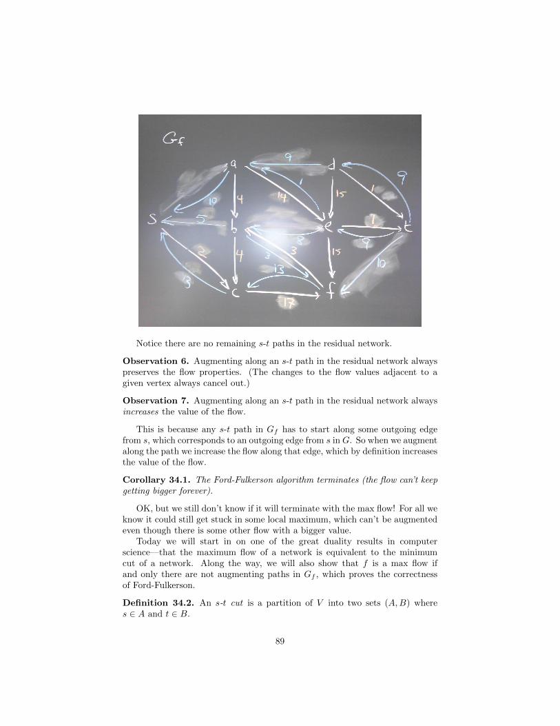
Notice there are no remaining s-t paths in the residual network.
Observation 6. Augmenting along an s-t path in the residual network alwayspreserves the flow properties. (The changes to the flow values adjacent to agiven vertex always cancel out.)
Observation 7. Augmenting along an s-t path in the residual network alwaysincreases the value of the flow.
This is because any s-t path in Gf has to start along some outgoing edgefrom s, which corresponds to an outgoing edge from s in G. So when we augmentalong the path we increase the flow along that edge, which by definition increasesthe value of the flow.
Corollary 34.1. The Ford-Fulkerson algorithm terminates (the flow can’t keepgetting bigger forever).
OK, but we still don’t know if it will terminate with the max flow! For all weknow it could still get stuck in some local maximum, which can’t be augmentedeven though there is some other flow with a bigger value.
Today we will start in on one of the great duality results in computerscience—that the maximum flow of a network is equivalent to the minimumcut of a network. Along the way, we will also show that f is a max flow ifand only there are not augmenting paths in Gf , which proves the correctnessof Ford-Fulkerson.
Definition 34.2. An s-t cut is a partition of V into two sets (A,B) wheres ∈ A and t ∈ B.
89

Definition 34.3. The capacity of an s-t cut is the total capacity of all edgescrossing the cut, that is,
c(A,B) =∑
e leaving A
c(e).
(Of course if an edge leaves A then it must enter B, that is, cross the cut.)
Show some examples—one “nice” and one crazy. Examine capacity of each.
Definition 34.4. The min cut is the s-t cut with minimum capacity.
Definition 34.5. The net flow of a cut (A,B) with respect to a flow f is∑e leaving A
f(e)−∑
e entering A
f(e),
i.e. the difference between the flow leaving A and the flow entering A. (Wecould thus call it A’s “net exports”.)
If we imagine the vertices of A being “clumped together” around the sourcevertex, then it’s clear what should happen: there will be no flow coming in toA, and the flow going out will just be equal to the value of the flow. But Acould be crazier—it could consist of a bunch of vertices scattered all throughthe graph. They don’t even have to be connected. So what can we say aboutthe net flow in general? Do some examples!
35 (L) Network flow: max flow/min cut
Lemma 35.1 (Flow Value Lemma). Let f be any flow and let (A,B) be anys-t cut. Then the net flow of (A,B) with respect to f equals the value of f .
Proof.
v(f) = fout(s) (1)
=∑v∈A
(fout(v)− f in(v)) (2)
=∑
e leaving A
f(e)−∑
e entering A
f(e) (3)
= net flow of (A,B) (4)
Line 2 follows because fout(v) = f in(v) for all v ∈ A besides s. (Rememberthat t /∈ A.)
To go from line 2 to line 3, consider all the edges with at least one endpointin A.
90
• If an edge has both endpoints in A, its flow contributes twice to the sumin line 2, once positively and once negatively, and the two cancel out.(Intuitively: moving stuff around within A does not affect its net exports.)
• Edges leaving A contribute positively to the sum.
• Edges entering A contribute negatively to the sum.
Hence we are left with line 3. Line 4 follows since line 3 is just the definition ofnet flow. SDG
Lemma 35.2 (Bottleneck Lemma). Let f be any flow and (A,B) be any s-tcut. Then v(f) ≤ c(A,B).
Proof.
v(f) =∑
e leaving A
f(e) −∑
e entering A
f(e)
≤∑
e leaving A
f(e)
≤∑
e leaving A
c(e)
= c(A,B)
SDG
Remark. From the proof we can see that v(f) = c(A,B) exactly when (1) thereis no flow entering A and (2) every edge leaving A is at max capacity.
Corollary 35.3. Given some flow f and s-t cut (A,B), if v(f) = c(A,B) thenf is a max flow and (A,B) is a min cut.
Proof. No other flow f ′ could be bigger than f since v(f ′) ≤ c(A,B). Likewise,no other cut could have smaller capacity than (A,B), since it has to be at leastas big as the value of f . SDG
Theorem 35.4 (Max flow/min cut). Let f be any flow on a network G. Thefollowing are equivalent:
1. v(f) = c(A,B) for some cut (A,B).
2. f is a max flow.
3. There are no s-t paths in the residual network Gf .
Proof. We will prove that 1⇒ 2⇒ 3⇒ 1.
• 1⇒ 2 is just Corollary 35.3.
• 2⇒ 3 because of Observation 7: if there were an s-t path in Gf , then wecould increase the flow along that path, so f would not be a max flow.
91

(3⇒ 1) is more interesting. Define an s-t cut (A,B) as follows:
• A = all nodes reachable from s in Gf .
• B = everything else.
Notice that
• s ∈ A (s is trivially reachable from itself).
• t ∈ B (t can’t be in A, since we assumed there are no s-t paths in Gf ).
By the Flow Value Lemma,
v(f) = net flow of (A,B) =∑
e leaving A
f(e) −∑
e entering A
f(e)
Note that each edge (u, v) leaving A must be filled to capacity, since other-wise there would be a forwards edge from u to v with the remaining capacity inGf , but then by definition we would have v ∈ A. Similarly, each edge enteringA must have 0 flow since if it didn’t, there would be a backwards edge from vto u in Gf , and then u would be in A.
Hence, we have
v(f) =∑
e leaving A
f(e) −∑
e entering A
f(e) =∑
e leaving A
c(e) = c(A,B).
SDG
Corollary 35.5. The Ford-Fulkerson algorithm is correct.
Proof. We already know Ford-Fulkerson terminates, and it ends when there areno s-t paths in Gf . By the theorem, this means it has found a max flow f . SDG
The proof of the max flow/min cut theorem actually shows something more:the Ford-Fulkerson algorithm can also be used as an algorithm to find a mincut. Just run the algorithm until it stops, and then do a DFS or BFS from s inthe residual network Gf to find all the connected vertices, which make up oneside of the min cut.
Bonus section: applications of network flow
• Maximum bipartite matching: given an arbitrary bipartite graph withedges between two sets of vertices L and R, we want to find a matchingwith the most number of edges. Solution:
– Add a new source vertex s with an edge to each vertex in L
92

– Add a new sink vertex t with an edge from each vertex in R
– Give every edge a capacity of 1.
The maximum flow now gives us a maximum matching.
Do an example—see how finding augmenting paths corresponds to findingzig-zagging paths and swapping which edges have flow and which don’t,so the number of edges with flow increases by 1 on each iteration.
• Assigning people to teams:
– Each pereson has teams they are willing to be on
– Each team has a max size
– Assign as many people as possible.
Bonus section: max flow algorithms in practice
Ford-Fulkerson is actually a kind of meta-algorithm: it specifies the methodof repeatedly augmenting along s-t paths in the residual network (augmentingpaths) but it doesn’t actually specify how to find augmenting paths. Withoutspecifying how to find augmenting paths at all, we can prove (on the HW) thatFord-Fulkerson will run in O(EC) time, where E is the number of edges and Cis the total capacity leaving the source (or the total capacity entering the sink,whichever is smaller). But if we are more careful about how we find augmentingpaths we can do better.
• The most straightforward way is to simply use a DFS from s to t in theresidual network. This works fine but not particularly well; depending onthe graph it can exhibit the worst case O(EC) behavior.
• We can use BFS in the residual network to find the shortest augmentingpath on each iteration. This is called the Edmonds-Karp algorithm, andit can be shown (though the proof is outside the scope of this course) thatit runs in O(V E2)—in particular, the running time does not depend onthe capacities. This algorithm works very well in practice, and often runsmuch faster than the worst case, behaving more like Θ(E3/2).
• We could use a variant of Dijkstra’s algorithm to find the maximum ca-pacity augmenting path on each iteration. This seems like it would be agood idea, but in practice it is usually slower than Edmonds-Karp.
• Finally, there is a clever method, Dinitz’ Algorithm, which instead of find-ing just a single augmenting path each iteration, sends flow along multipleaugmenting paths at once. (Note: it is often known as Dinic’s Algorithm,but this is due to a misspelling of the name of its inventor, Yefim Dinitz.)It works as follows:
1. Do a BFS from s in the residual network and label every vertex withits level in the BFS tree.
93

2. Now do a DFS from s in the residual network, only taking edges whichgo from level i to i+ 1; as we recurse through the graph, keep trackof the available flow and the minimum residual capacity along thepath to each point. Once we reach s we can unroll the recursion andupdate flow values with the minimum capacity seen along the path,and subtract the augmenting flow from the available flow. Instead ofstopping, however, we keep going to try to augment along as manypaths as we can. If we encounter a vertex from which it’s impossibleto reach t, we mark it so we know not to visit it if we ever encounterit again.
It can be shown that this takes O(V 2E), an improvement over Edmonds-Karp for dense graphs; Dinitz also works very well in practice and typicallyruns much faster than O(V 2E). Also, when using max flow to compute amaximum matching in a bipartite graph, it can be shown that Dinitz runsin O(E
√V ) (this special case of Dinitz for maximum bipartite matching
was invented independently and is known as Hopcroft-Karp).
There are many other approaches to finding maximum flows as well (preflow-push, push-relabel, simplex. . . ), which can have even better asymptotic runningtimes, work better on certain types of graph, or solve more complex max flowvariants (max circulation, min-cost max flow, . . . ), but for most practical maxflow problems you will encounter, Edmonds-Karp or Dinitz should work justfine!
94

36 (P*) Intro to reductions: Independent setand vertex cover
95

37 (L) Intro to intractability: reductions
This week we will begin studying the limits of computation, from an algorithmicperspective. What problems can computers solve, and what problems can’t theysolve? Which problems can be solved efficiently and which can’t?
The main tool we will use is the process of reduction. Suppose we have analgorithm to solve problem B, which we can think of as a black box that takessome inputs describing a problem instance and yields an appropriate output:
B
We can think of our algorithm as a “subroutine” to turn it into a solutionto another problem:
g(y)yB
f(x)
A
x
• The function f translates inputs for problem A into inputs for problemB.
• The function g translates outputs for problem B into outputs for prolemA.
• Note we can even allow multiple “calls” to B.
Of course, this is only useful if this really does solve problem A. That is,we need the property that if y is a solution of problem B for input f(x), theng(y) is a solution of problem A for input x. In this case we write A ≤ B (“A isreducible to B”). Note we can prove such a reduction without having an actualalgorithm to solve problem B: we just show that if we had an algorithm to solveB then we could also use it to solve A.
Let’s do an example.
Independent set
Definition 37.1. An independent set in an undirected graph G = (V,E) is aset of vertices S ⊆ V such that no two nodes in S are joined by an edge.
For example:
6
3
1 2
5
7
4
96
What independent sets can you find? Finding small independent sets isrelatively easy: for example, any set consisting of just a single vertex is anindependent set by definition. Any two vertices that are not connected by anedge also form an independent set, like 1, 7. Clearly, the interesting thing is totry to find large independent sets. In this particular example, we can convinceourselves that the largest independent set is of size 4, namely, 1, 6, 4, 5. Howhard is it in general to find the largest independent set? At this point, it’s notclear! A brute force solution (look at every subset of vertices and check whethereach is independent) will obviously take Ω(2n) if n is the number of vertices.
Instead of simply asking for the largest independent set, we are going tophrase the problem as a decision problem, which asks for a yes/no answer.(We’ll explore the reasons for this later.)
Independent-Set: Given a graph G and a natural number k, does Gcontain an independent set of size at least k?
Vertex cover
Now let’s consider another problem.
Definition 37.2. A vertex cover in a graph G = (V,E) is a set S ⊆ V suchthat every e ∈ E has at least one endpoint in S. (In other words, each e ∈ E is“covered” by some v ∈ S.)
Look at our example graph from before. It’s easy to find large vertex covers(for example, the set of all vertices is obviously a valid cover) but hard to findsmall ones. For our example graph we can convince ourselves that the smallestvertex cover has size 3 (namely, 2, 3, 7).
Vertex-Cover: Given a graph G and a natural integer k, does Gcontain a vertex cover of size at most k?
As you may have intuited from our example, there is a close relationshipbetween Independent-Set and Vertex-Cover.
Theorem 37.3. Let G = (V,E) be an undirected graph. Then S ⊆ V is anindependent set if and only if V − S is a vertex cover.
Proof. (=⇒) Let S be an independent set. We must show V − S is a vertexcover. So let e = (u, v) ∈ E. We must show at least one of u or v is in V − S.But since S is an independent set, u and v can’t both be in S; so at least oneof them is not in S, that is, in V − S.
(⇐=) Let V − S be a vertex cover; we must show S is an independent set.So let u, v ∈ S; we must show there is no edge connecting them. Since u, v ∈ Sthen neither one is in V −S. Hence there cannot be an edge (u, v), since V −S
97

is a vertex cover, and so every edge must have at least one of its endpoints inV − S. SDG
Corollary 37.4. Independent-Set ≤ Vertex-Cover and Vertex-Cover ≤Independent-Set.
Proof. Suppose we have an algorithm to solve Vertex-Cover. Then to solveIndependent-Set(G, k), just solve Vertex-Cover(G,n− k): G has an inde-pendent set of size at least k if and only if it has a vertex cover of size at mostn− k. The other direction is similar. SDG
98

38 (P/L) Satisfiability
Suppose we are given a set X = x1, . . . , xn of Boolean variables.
Definition 38.1. A term is either a variable xi, or the logical negation of avariable, which we write xi (the negation of xi is also often written ¬xi).
Definition 38.2. A clause is a disjunction of one or more terms, t1 ∨ · · · ∨ tl.
For example, x1 ∨x3 ∨x4 is a clause. (Note there’s nothing in the definitionprecluding repeated variables like x1∨x1∨x1∨x3, but such repetition does notadd anything from a logical point of view, so we usually think of the variablesas being distinct.)
Definition 38.3. A truth assignment is a function X → T,F assigning avalue of true or false to each variable xi. A truth assignment satisfies a clauseC if it causes C to evaluate to true (under the usual rules of Boolean logic).
For example, x1 7→ T, x2 7→ F, x3 7→ F, x4 7→ F satisfies x1 ∨ x3 ∨ x4, butx1 7→ F, x2 7→ F, x3 7→ T, x4 7→ F does not.
Definition 38.4. A truth assignment v : X → T,F satisfies a collection ofclauses C1, . . . , Ck if it satisfies all of them (that is, it satisfies C1∧C2∧· · ·∧Ck).We say that v is a satisfying assignment for C1, . . . , Ck. When a collection ofclauses has some satisfying assignment, we say it is satisfiable.
For example, (x1 ∨ x2), (x1 ∨ x3), (x2 ∨ x3) is satisfiable: just set all xi to F.(This is not the only possible satisfying assignment.)
On the other hand, as you can verify, x1, (x3∨x1), (x3∨x1) is not satisfiable:there is no way to assign truth values to the xi which will simultaneously satisfyall the clauses.
Given these definitions, we can state the following problems:
Satisfiability (SAT): Given clauses C1, . . . , Ck over the variables X =x1, . . . , xn, is the collection of clauses satisfiable?
Here is another variant of SAT which seems like it might be easier:
3-SAT: Given a collection of clauses C1, . . . , Ck each containing exactlythree variables, is it satisfiable?
Obviously we have
Theorem 38.5. 3-SAT ≤ SAT.
99

Proof. Since 3-SAT is just a special case of SAT, if we could solve SAT thenwe could solve 3-SAT as well; we wouldn’t even have to do any conversion atall. SDG
Remark. It turns out (but is extremely nonobvious!) that the other direction istrue as well: SAT ≤ 3-SAT (we will prove this eventually). So in some senseeven though the special case of 3-SAT seems like it might be “easier” than thegeneral case of SAT, it is not.
Why 3, you ask? Because 3 is the smallest k for which k-SAT is just as hardas SAT. It turns out that 2-SAT, where all clauses have exactly two variables, ismuch easier, and can even be solved in linear time. (1-SAT, of course, is trivial(though not as trivial as 0-SAT).)
Now let’s connect these problems back to some of the problems we haveconsidered previously.
Theorem 38.6. 3-SAT ≤ Independent-Set.
Proof. We want to exhibit a polynomial-time reduction from 3-SAT to Independent-Set. That is, given a black box to solve Independent-Set, we want to showhow we could use it to solve 3-SAT, using only a polynomial amount of addi-tional work.
Given a set of 3-SAT clauses, we want to find a satisfying assignment, whichhas to make each clause true. In order to make a clause true it suffices tochoose exactly one term from each clause which will be set to T. (Note that“setting xi to True” of course means setting xi to F.) However, we have tochoose consistently: we can never pick both xi and xi.
We start by constructing a graph G with 3k vertices arranged in k triangles,like so:
vk3vk2
vk1
v23v22
v21
v13v12
v11
Each triangle corresponds to a clause, and each vertex corresponds to a term;in particular, label vij by the jth term from clause Ci. So, for example, giventhe clauses
(x1 ∨ x3 ∨ x4), (x2 ∨ x1 ∨ x3), (x1 ∨ x3 ∨ x4),
we would start by constructing the graph
100

x4x3
x1
x3x1
x2
x4x3
x1
This graph always has independent sets of size k (but no bigger): just pickexactly one node from each triangle. However, we don’t want to allow pickingjust any old combination of nodes. So we add more edges: in particular, addan edge between every pair of nodes labelled by xi and xi for some i. So ourexample graph becomes:
x4x3
x1
x3x1
x2
x4x3
x1
An independent set can’t contain both endpoints of an edge. These edgestherefore encode the constraint that we have to choose variables consistently:we can never choose both xi and xi.
The claim is now that this graph has an independent set of size ≥ k iffthe original 3-SAT instance is satisfiable—and hence we can solve the original3-SAT instance by asking our black box for Independent-Set whether thisgraph has an independent set of size ≥ k. If the graph has an independent setof size ≥ k, it must in fact have size exactly k and consist of a choice of oneterm from each clause. Just making these terms T will result in a satisfyingassignment (variables which do not correspond to any chosen term can be setto anything, say, F); this is well-defined because we will never have both xiand xi selected (because of the extra edges we added). Conversely, if there isa satisfying assignment, just choose one vertex from each triangle whose labelis T under the assignment (since it is a satisfying assignment, each clause musthave at least one term which is T). Any two vertices connected by an edge areeither in the same triangle (and we only pick one vertex from each triangle) orare labelled with inverse terms (and hence can’t both be labelled T), so this isan independent set of size k.
SDG
At this point, we have shown
3-SAT ≤ Independent-Set ≤ Vertex-Cover.
101

39 (L) Decision problems and the ≤P relation
Definition 39.1. We say an algorithm takes polynomial time if it runs in O(nc)for some constant c, where n is the size of the input.
Remark. Note this doesn’t mean the running time has to look like a polynomial!For example, an algorithm that takes time Θ(n2 log n) is polynomial-time, sinceit runs in, e.g., O(n3).
Definition 39.2. If A ≤ B and the translation functions f and g take poly-nomial time to compute, and the reduction makes only a polynomial numberof subroutine calls to B, then we say that A is polynomial-time reducible to B,and write
A ≤P B.
Remark. Why focus on polynomial time in particular? Several reasons:
• Polynomials are closed under a lot of natural operations:
– addition (corresponding to running algorithms in sequence),
– multiplication (corresponding to calling one algorithm as a subrou-tine of another),
– and even substitution (corresponding to algorithm composition, thatis, using the output of one algorithm as the input to another).
This means that if we have two polynomial-time algorithms and combinethem in some way, the result will also take polynomial time.
• Empirically, polynomial time corresponds well to what is feasible in prac-tice.
Decision problems
Notice how Independent-Set and Vertex-Cover are formulated to give ayes/no answer, i.e. a single bit of information. Such problems are called decisionproblems. Note that when reducing decision problems we don’t have to worryabout translating the output (except perhaps to negate it).
It might seem limiting to restrict ourselves to only decision problems, butactually it is not as restrictive as you might think. As an example, consideranother variant of Independent-Set:
Independent-Set -Opt: Given an undirected graphG, find the largestnatural number k such that G has an independent set of size k.
Clearly Independent-Set ≤P Independent-Set-Opt: to decide whetherG has an independent set of size at least k, just find the size of the largestindependent set and compare it to k. But actually, Independent-Set-Opt ≤P
102

Independent-Set as well! To find the largest size of an independent set, wecan call Independent-Set as a subroutine for each k from 1 up to n until wefind the biggest for which we get a “yes” answer. Or we could even be a bit(haha) more sophisticated and do a binary search: Independent-Set returnsa single bit as an answer, and using binary search we can reveal a single bit ofthe desired solution k with each subroutine call to Independent-Set. Thisresults in only a polynomial number (Θ(n) or Θ(log n)) of subroutine calls.
This sort of relationship holds often. So, because they are simpler to dealwith and don’t actually restrict us that much, we will just work in terms ofdecision problems.
Lemma 39.3. Suppose A and B are decision problems with A ≤P B. If B issolvable in polynomial time, then so is A.
Proof. Suppose we have an input x to A of size n. Suppose the translationfunction f (which converts x into an input suitable for B) takes time p(n) tocompute, for some polynomial p. Note that this means the size of f ’s output isalso O(p(n)), since it takes p(n) time and it has to produce the entire output inthat time.
Now suppose B can be solved in time q(m), where q is a polynomial andm is the size of its input. Then the total time to solve problem A on input x,using the reduction to B, is the time to convert the input plus the time to runB on an input of size O(p(n)), that is,
p(n) + q(p(n)).
Since p and q are polynomials, and polynomials are closed under addition andsubstitution, this is a polynomial. SDG
Remark. It is not too hard to extend this in a couple ways:
• If A and B are not decision problems then we must also take into accountthe time needed to run the output conversion.
• We can also take into account the case where B is called a polynomialnumber of times as a subroutine—it essentially involves multiplying byanother polynomial, though to do it formally one has to be a bit morecareful to state that we have not just a single input conversion functionbut many, which are all bounded by some polynomial runtime.
Corollary 39.4. Suppose A ≤P B. If A is not solvable in polynomial time,then neither is B.
Intuitively, if A ≤P B then B is “at least as hard as” A (that is, with respectto solvability in polynomial time).
Lemma 39.5. ≤P is reflexive and transitive.
103

Proof. We can easily reduce a problem to itself using identity conversion func-tions, which are obviously polynomial-time. Also, if A ≤ B and B ≤ C it iseasy to see that A ≤ C by nesting the reductions. A bit more work is requiredto show that the resulting nested reduction will still be polynomial, but it againboils down to the fact that polynomials are closed under substitution. SDG
104
40 (L) NP
Often, problems which seem hard to solve can nonetheless be easy to verify ifwe are handed a (potential) solution. For example, consider the Independent-Set problem. We don’t yet know how hard it is to solve, but if someone handsyou a set which they claim is an independent set of size ≤ k, it is easy to verifywhether it has the desired size and is, in fact, an independent set—just checkeach pair of vertices in the set to see whether they are connected by an edge.3-SAT is similar: if someone hands you a variable assignment, all you have todo is plug it in and evaluate the clauses to see whether they are all satisfied.
Let’s be a bit more formal. We will suppose that the input to a problem isencoded as a binary string s. Formally, the “size” of the input will now be thenumber of bits, n = |s|. We will also identify a decision problem X with the setof all inputs s for which the answer should be “yes”. The problem then boilsdown to deciding whether a given bitstring s is contained in X or not. (This isanother reason why studying decision problems is particularly nice.)
Definition 40.1. An algorithm A solves X if for all binary strings s, A(s) = Tiff s ∈ X.
(If we wanted to be even more formal, we should identify an “algorithm”with some concrete model of computation, typically a Turing machine.)
Definition 40.2. If there is a polynomial p(n) such that A(s) always terminatesin at most p(|s|) steps, we say A is a polynomial-time algorithm and write A ∈ P.
Now let’s formally define what it means to be able to verify the solution toa decision problem. The idea is that we need some sort of extra information toverify a positive answer to a decision problem. For example, given some largegraph, if someone were to claim that there was a vertex cover of size ≤ 20, youwould challenge them to prove it to you by showing you the vertex cover. Givenan actual set of vertices, it would be easy for you to check that the set hassize ≤ 20 and also that every edge in the graph is covered. Conversely, if thereis no vertex cover of that size, then no one is going to be able to fool you bygiving you some weird set of vertices. The extra information required to verifya solution is called a certificate.
Definition 40.3. An algorithm B is a polynomial-time certifier for a decisionproblem X if:
• B is a polynomial-time algorithm taking some inputs s and t
• There is a polynomial p such that for all bitstrings s, we have s ∈ X ifand only if there is some bitstring t (called a certificate) with |t| ≤ p(|s|)and B(s, t) = T.
In other words, s ∈ X if and only if there is a (not too big) certificate“proving” it, which can be efficiently checked. That is, if the answer to the
105

decision problem s ∈ X is YES, then there is a certificate t that proves it: thecertifier algorithm B, when run on s and t, will return T. Conversely, if s /∈ X,there is no t that works: B will never return T for a certificate t unless s reallyis in X.
For example, again thinking about Vertex-Cover, s is of course a descrip-tion of a graph and a number k; a certificate t is simply a list of vertices; thealgorithm B checks whether the given set of vertices is ≤ k and whether everyedge is covered by some vertex in the set, which clearly takes time polynomialin the size of the graph.
Definition 40.4. If X has a polynomial-time certifier, we say X ∈ NP.
For example, 3-SAT, Vertex-Cover, and Independent-Set ∈ NP ac-cording to our discussion above.
Remark. NP stands for “nondeterministic polynomial time”. The idea is thatif we could make nondeterministic choices (i.e. choose multiple things at onceand try them in parallel), we could solve any NP problem in polynomial time:just nondeterministically make all possible choices for the certificate t and checkthem all at the same time.
We can also observe that
Proposition 40.5. P ⊆ NP.
Proof. Given a decision problem which can be solved in polynomial time, wecan construct a polynomial-time verifier B which simply ignores the certificateand runs the polynomial-time algorithm to solve the problem. SDG
Question. Does P = NP? This question is literally worth $1 million (it is oneof the seven “Millenium Prize Problems” published by the Clay MathematicsInstitute). It seems too good to be true, and most believe the answer is no. Butthis seems extremely difficult to prove.
Definition 40.6. A decision problem X is NP-hard if for all Y ∈ NP, Y ≤P
X.
Intuitively, a problem is NP-hard if it is “at least as hard as everything inNP”. It seems reasonable that there might be some extremely hard problemswhich fit the bill—though how on earth would we go about proving it? To showthat X is NP-hard, we have to somehow show that every NP problem can bereduced to X, which at first glance seems impossible.
Lemma 40.7. If X is NP-hard and X ≤P Y then Y is NP-hard.
Proof. Transitivity of ≤P . SDG
So if we can find just one NP-hard problem, we can potentially use thislemma to find others.
Definition 40.8. A decision problem X is NP-complete if both X ∈ NP andX is NP-hard.
106
It is not at all clear that any such problems exist at all! We could just aseasily imagine a situation where there are just a bunch of problems in NP whichare “maximally hard”—that is, no other problems in NP are harder—but arestill not harder than everything in NP. Or we could imagine that the onlyproblems harder than everything in NP are themselves so hard that they arenot in NP.
Proposition 40.9. If a decision problem X is NP-complete, then X is solvablein polynomial time if and only if P = NP.
Proof. (=⇒) If X is solvable in polynomial time, then by a previous lemma, anyY with Y ≤P X is also solvable in polynomial time. But if X is NP-completethen by definition every problem in NP is reducible to X and hence solvable inpolynomial time.
(⇐=) If X is NP-complete then by definition X ∈ NP, so if P = NP thenX ∈ P. SDG
Corollary 40.10. If you come up with a polynomial-time algorithm to solve anNP-complete problem, you win $1 million.
Good luck. Note that this is not just theoretical; it turns out that thereare a great many NP-complete problems that people actually care about on apractical level. So lots of smart people have been trying hard for a long time todevelop good algorithms to solve them, but no one has ever come up with anypolynomial-time algorithms for any of them.
107

41 (L) The first NP-complete problem
Definition 41.1. A boolean circuit is a directed, acyclic graph G such that:
• Each indegree-0 vertex (“input”) is labelled with either F, T, or a distinctvariable.
• All other vertices have indegree 1 or 2, and are labelled with either ¬ (ifindegree 1) or ∨ or ∧ (if indegree 2)
• Only one vertex has outdegree 0, which we call the “output”.
(Note this is not really a “circuit” as we would usually conceive it, since inparticular there are no loops!)
Given a truth assignment for the variables labelling the inputs, we think ofthe circuit as resulting in a T/F value in the obvious way: each edge correspondsto a wire which carries a single T/F value to the input of the next logic gate.Boolean circuits come with a natural decision problem:
Circuit-SAT: Given a boolean circuit, is there an assignment of theinput variables such that the circuit outputs T?
Theorem 41.2 (Cook, Levin (1971)). Circuit-SAT is NP-complete.
Proof. First, it is easy to see that Circuit-SAT ∈ NP: a certificate is a truthassignment; to verify it we can just run the circuit and check that it outputs T.
Now we must show Circuit-SAT is NP-hard. Suppose X ∈ NP, i.e. Xhas a polynomial-time certifier B. We must show X ≤P Circuit-SAT.
Since B is an algorithm, it can be encoded as a boolean circuit (proof:computers exist, and any boolean function can be encoded using ∧, ∨, ¬).Well, except for one problem: our boolean circuits have no loops. But we cancircumvent that by simply “unrolling” any loops, by making a whole bunchof copies of a circuit that computes a single step. If the algorithm only runsfor a polynomial amount of time then we need at most a polynomial numberof copies to make this work. So, intuitively, we can build a polynomial-sizedboolean circuit that simulates the algorithm B. Given an input s, we fix theinputs corresponding to s, and leave as variables the inputs corresponding to t.Now we ask whether the resulting circuit is satisfiable. If it is, that means thereis some t such that B(s, t) = T, that is, s ∈ X. If it is not satisfiable, then thereis no such t, so s /∈ X. Hence X ≤P Circuit-SAT. SDG
Now that we know there is one NP-hard problem, finding others is a lotsimpler!
Theorem 41.3. 3-SAT is NP-complete.
108

Proof. We already know 3-SAT ∈ NP. We will show it is also NP-hard “byreduction from Circuit-SAT”, that is, we will show Circuit-SAT ≤P 3-SAT.Since we know Circuit-SAT is NPoly-hard, by transitivity this will mean that3-SAT is also NP-hard.
We are given a circuit as input, and have to decide whether it is satisfiable.We will construct a corresponding 3-SAT instance which is satisfiable iff theoriginal circuit is.
First, associate a distinct variable with each edge in the circuit. Now we willdefine one or more clauses for each node, where each clause has at most threeterms. To make things a bit more intuitive we will use a ⇒ b as shorthand fora ∨ b.
• Given a ¬ node with input xu and output xv, generate the two clauses(xu ⇒ xv) and (xu ⇒ xv).
• Given a ∨ node with inputs xu, xv and output xw, generate the threeclauses (xu ⇒ xw), (xv ⇒ xw), and ((xu∧xv)⇒ xw) (this last expressionsimplifies to xu ∨ xv ∨ xw, so it is a valid clause; remember clauses cancontain only ∨, not ∧).
• Given a ∧ node with inputs xu, xv and output xw, generate the threeclauses (xu ⇒ xw), (xv ⇒ xw), and ((xu ∧ xv)⇒ xw) (which simplifies toxu ∨ xv ∨ xw).
• For a constant input node connected to the edge xu, just generate theclause xu (if the constant is T) or xu (if the constant is F).
• Finally, generate a clause containing just the variable connected to theoutput node (since we want the output to be true).
At this point it is clear that the resulting set of clauses will be satisfiable ifand only if the original circuit is satisfiable, because the clauses encode exactlywhat will be computed throughout the entire circuit.
The only remaining detail is that we have to make sure each clause hasexactly three terms. To do this, first introduce four new variables, call themz1 . . . z4. The idea is that we will force z1 and z2 to be F (z3 and z4 exist justto help us do this), so they can be used to “pad out” any clauses which are tooshort, without affecting their meaning.
Create eight new clauses of the form (zi ∨ ±z3 ∨ ±z4), where we replace ziby either z1 or z2, and replace ±z3 by either z3 or z3, and so on, and we do thisin all possible ways, thus resulting in eight clauses. Notice that these clausesforce z1 = z2 = F: no matter what values are assigned to z3 and z4, there willbe one clause of the form (z1 ∨ . . . ) where the . . . terms are false, and hence forthe clause to be satisfiable we must have z1 = F (and similarly for z2). Now,for each clause with fewer than three terms, just add · · · ∨ z1 or · · · ∨ z1 ∨ z2 asappropriate to bring it up to three terms. Since z1 and z2 must be F, this hasno effect: the new, padded clause will be satisfied iff the original clause is.
109

Hence we have succeeded in constructing a 3-SAT instance which is satisfi-able iff the original boolean circuit is satisfiable. The constructed 3-SAT instancehas as many variables as there are edges in the circuit, and no more than 3n+ 8clauses, where n is the number of vertices in the circuit, so constructing the3-SAT instance takes time polynomial in the size of the circuit. SDG
Corollary 41.4. 3-SAT, SAT, Independent-Set, and Vertex-Cover areall NP-complete.
Proof. We have already discussed the fact that they are NP. Since we nowknow Circuit-SAT ≤P 3-SAT ≤P Independent-Set ≤P Vertex-Coverand 3-SAT ≤P SAT, by transitivity of ≤P they are all NP-hard. SDG
This is amazing. Just by looking at the definitions it wasn’t at all clearwhether we would be able to find a single problem which was NP-complete,and now we have found five. (And you will find yet more on your HW.) In fact,it turns out that we currently know of hundreds of “natural” problems whichare NP-complete.
So, the “reason” Circuit-SAT is NP-hard is that we can use it to modelarbitrary computation, by essentially building a little computer. But thinkabout what this transitive chain of reductions is then showing us: we can takea circuit modelling a computer and reduce it to a 3-SAT instance which modelsthe same computer. But we can then in turn take that 3-SAT instance modellinga computer and reduce it to a graph, such that finding an independent set of acertain size in the graph models the same computation! Computation is sneakylike that; you end up finding it in places you would not expect. Who would haveguessed that finding independent sets in a graph turns out to be equivalent todoing arbitrary computation? But in some sense NP-complete problems arelike this, and this gives us some intuition as to why they are so hard to analyze:because you can smuggle arbitrary computation into them!
110

42 (L) Travelling salesman is NP-complete
1. 3-SAT ≤ HAMILTONIAN CIRCUIT ≤ TRAVELLING SALESMAN.
See K&T for reductions.
111

43 (L) Super Mario Bros (and Kirby’s DreamWorld) are NP-hard
Show paper by Aloupis et al.
112
44 (L*) Rabin-Karp pattern matching
Given a pattern P = p1 . . . pm and a text T = t1 . . . tn where pi, ti ∈ 0, 1,a natural question to ask is, does P occur as a substring within T (and if so,where)? Note that typically n is much larger than m; think of T as a largebody of text and P as a word or phrase we are looking for. (If we wanted todo this with actual text instead of bitstrings, we could simply encode the textas bitstrings, or all of the following can be easily generalized to alphabets otherthan 0, 1.)
Let Ti,m = titi+1 . . . ti+m−1 be the substring of T starting at index i withlength m (the same length as the pattern P ). The question then becomes: doesthe exists some 1 ≤ i ≤ n−m+ 1 such that Ti,m = P? Note that P must occurcontiguously (we are looking for a substring, not a subsequence).
The naıve algorithm would be to just try comparing P to each position inT , but this is O(nm) in the worst case (imagine matching P = 00001 againstT = 0000 . . . 0000). There are algorithms for solving this problem in O(n+m)such as Knuth-Morris-Pratt or Boyer-Moore. These algorithms are deterministicbut somewhat complicated. Today we will look at the Rabin-Karp algorithm,which involves randomness and has O(n + m) expected time. Even if m isrelatively small, this can make a big difference in practice (imagine if Googletook 14 times longer to search for an input phrase with 14 letters than it did tosearch for a single letter).
The idea is to use a hash function h. The basic outline of the algorithm isas follows:
Algorithm 15 Naıve Rabin-Karp
1: for i← 1 . . . n−m+ 1 do2: if h(Ti,m) = h(P ) then3: if Ti,m = P then return i
return Not found
We iterate through all possible positions, and check whether the hashes ofTi,m and P are equal. If the hashes are not equal then Ti,m and P definitely donot match. But if the hashes are equal, we still have to check, since differentstrings can hash to the same value.
Our hope is that by checking hashes we can avoid actually comparing strings.However, at this point we haven’t actually saved any work yet. The outer loop(line 1) of course executes O(n) times, and computing the hash of a length-mbitstring definitely takes at least Ω(m) time because it at least has to read thewhole string! So the whole algorithm is still O(mn). However, we have madesome conceptual (if not actual) progress!
The first insight is that if we pick h cleverly, we can avoid doing so muchwork to compute it: perhaps we can compute h(Ti+1,m) from h(Ti,m) in O(1)time. That would bring down the time needed for the check on line 2. The only
113

remaining problem is that we might have too many hash collisions. The checkon line 3 is still O(m); if we have to do the expensive equality check too manytimes, the algorithm could still be O(mn) overall. We’ll address this problemlater.
To be able to compute h incrementally in this way, we introduce the conceptof a rolling hash function.
Definition 44.1. Let I(b1 . . . bm) = 2m−1b1 + 2m−2b2 + · · ·+ 20bm, that is, theinteger value of b1 . . . bm considered as a binary number.
Definition 44.2. Let p be a prime number chosen from some range [1 . . . 2k](we will pick k later). Then define hp(X) = I(X) mod p.
Note that hp(X) takes O(m) time to compute (where m is the number ofbits in X).
Notice that
I(Ti+1,m) = I(ti+1ti+2 . . . ti+m)
= 2m−1ti+1 + 2m−2ti+2 + · · ·+ 21ti+m−1 + 20ti+m
= 2mti + 2m−1ti+1 + · · ·+ 21ti+m−1 − 2mti + 20ti+m
= 2(2m−1ti + 2m−2ti+1 + · · ·+ 20ti+m−1)− 2mti + ti+m
= 2I(titi+1 . . . ti+m−1)− 2mti + ti+m.
and hence hp(Ti+1,m) = (2hp(Ti,m) − 2mti + ti+m) mod p, which can be com-puted in O(1). So now the initial evaluation of hp(T1,m) takes O(m), andcomputing subsequent values of hp takes only O(1).
Now, what about collisions? Note that
hp(P ) = hp(Ti,m)
⇐⇒ I(P ) ≡ I(Ti,m) (mod p)
⇐⇒ I(P )− I(Ti,m) ≡ 0 (mod p)
⇐⇒ p divides |I(P )− I(Ti,m)|.
Since both P and Ti,m have m bits, their difference is at most |I(P )−I(Ti,m)| ≤2m. So we can quantify the probability of a hash collision by answering twoquestions:
1. How many prime divisors can a number ≤ 2m have?
2. How many primes are there in the range [1, 2k]?
Answering the first question is easy:
Lemma 44.3. Any number N ≤ 2m has at most m distinct prime divisors.
Proof. All primes are ≥ 2. So if there were more than m distinct prime divisors,their product would be > 2m. SDG
114

The second question is not so easy to answer, but thankfully it has alreadybeen answered for us:
Theorem 44.4 (Prime number theorem). Let n ∈ Z+, and let π(n) denote thenumber of primes ≤ n.
π(n) = Θ( n
lnn
).
We can now quantify the probability of a hash collision, which is just theprobability that the chosen prime p matches one of the prime divisors of I(P )−I(Ti,m). This probability, in turn, is just the number of distinct prime divisorsof I(P )− I(Ti,m) divided by the total number of primes in [1, 2k].
Pr[hp(P ) = hp(Ti,m,)] =# of distinct prime divisors of I(P )− I(Ti,m)
# of primes ∈ [1, 2k]
≤ m
π(2k)
= O
(m
2k/ ln 2k
)= O
(mk
2k
)If we choose 2k = nm log(nm), then k = log 2k = log(nm) + log log(nm) ≤
2 log(nm) = O(log(nm)), in which case
O
(mk
2k
)= O
(m log(nm)
nm log(nm)
)= O(1/n).
Therefore the probability of getting a collision at each index i is only 1/n, whichmeans we expect about 1 collision over the course of the entire algorithm—thisis great! The whole algorithm thus runs in O(m + n) (O(m) to compute theinitial hash + O(n) loops with O(1) work in each to compute the next hash +O(m) to do the expected 1 equality check).
And finally, how big is p? Actually it’s not bad at all: p has k = O(log(nm)) =O(log n) bits. For example, a 64-bit prime is enough to efficiently search in atext of 264 bits ≈ 2 exabytes.
115

45 (L*) Bucket sort
Suppose we are given a list of 10 million records, each representing a person,and we want to sort them by their birthday (i.e. all the people born on January1st come first—regardless of their birth year—then all those born on January2nd, and so on). What is the best algorithm for doing this?
We could of course use a standard sorting algorithm like merge sort, whichwould take Θ(n log n) time. But in this case we can actually do somethingbetter! Make an array with 366 “buckets”, one for each day of the year. Nowscan through the records and put each record in the bucket corresponding to itsbirthday. After putting all the records in buckets, simply list all the items inthe first bucket, followed by all the items in the second, and so on. Assumingthat we can add and remove from the buckets in constant time, and that we canaccess any given bucket in constant time, this algorithm takes only Θ(n) time.
So what gives? Haven’t we proved that we can’t sort any faster thanΘ(n log n)? Well, yes, but that is for comparison-based sorting, i.e. sortingunder the assumption that the only thing we can do with two keys is to com-pare them. In this case we can do better, since we know in advance how manykeys there are and can easily convert them into consecutive integers.
In general, if we have a list of items L with |L| = n, and k different keys0 . . . k − 1, we can use the following algorithm:
Algorithm 16 Bucket Sort(S)
1: Initialize an array Q of k queues2: for x ∈ L do3: Add x to Q[x.key ]
4: for i ∈ 0 . . . k − 1 do5: Append the contents of Q[i] to the output list
We assume we are using a queue implementation that supports Θ(1) enqueueand dequeue. This algorithm takes Θ(k) to create the buckets in the first place,then Θ(n) to scan through and place everything in buckets, and another Θ(n)to list the buckets in order, for a total of Θ(n+ k). This works well when
• we know k in advance
• k is relatively small
Of course if k < n this is Θ(n).Using queues for buckets ensures that the algorithm is stable: we say a
sorting algorithm is stable if items having equal keys retain their relative orderfrom the input. All the items with a given key i are added to Q[i] in the orderthey are encountered in the input list L, and then removed from Q[i] in thesame order. This stability may or may not be a big deal when using bucketsort by itself—we might not care about the relative ordering of all the people
116

born on February 12—but it will turn out to be crucial in using bucket sort asa building block for more complex algorithms.
117

46 (L*) Radix sort
Suppose more generally that our keys are strings in Σ∗ for some alphabet Σ,that is, keys are sequences of elements from Σ. For example, if Σ = 0, . . . , 9then keys would be numbers like 123 or 97268. If the keys have length up to dthen there are |Σ|d| possible keys, which is probably too many to do bucket sort.For example, suppose we have ten million records which we want to sort by lastname, where each name is a string of letters. Even if we assume that names areat most ten letters long (probably a bad assumption!), that is still 2610 ≈ 141trillion possible names, so bucket sort—which would require creating an arraywith 141 trillion elements—is completely out of the question.
However, in this situation we can still often do better than a comparison-based sort, using an algorithm called radix sort. Radix sort was actually usedas long ago as 1887 (yes, 1887, not 1987); look up Herman Hollerith if you wantto know more!
The basic idea is to do an independent bucket sort on each key position. Asan example, suppose Σ = 0, . . . , 9, and let’s begin with the list
126, 328A, 636, 128, 341, 121, 416, 131, 016, 328B .
The two copies of 328 are marked with A and B so we can see what happens tothem.
• First, we bucket sort on the least significant, i.e. last, digits. We wouldput 126 into the 6 bucket, then 328A into the 8 bucket, and so on, resultingin the buckets
0 1 2 3 4 5 6 7 8 9341 126 328A121 636 128131 416 328B
016
So, after listing out all the buckets in order, we get
341, 121, 131, 126, 636, 416, 016, 328A, 128, 328B .
• Next, we bucket sort on the second digit:
0 1 2 3 4 5 6 7 8 9416 121 131 341016 126 636
328A128
328B
resulting in
416, 016, 121, 126, 328A, 128, 328B , 131, 636, 341.
118

The bucket sort puts the elements in order by their second digit, but noticethat something else has happened: because they were already sorted bytheir last digit, and bucket sort is stable, elements with the same seconddigit end up in the correct order with respect to their last digits. So atthis point, the list is actually sorted by the last two digits of each element(16, 16, 21, 26, 28, . . . ).
• One final bucket sort by the first digit now leaves the entire list correctlysorted:
0 1 2 3 4 5 6 7 8 9016 121 328A 416 636
126 328B128 341131
resulting in
016, 121, 126, 128, 131, 328A, 328B , 341, 416, 636.
Again, since the elements were already correctly sorted by their last twodigits, doing a stable sort on their first digits leaves them in the correctorder. Notice also that radix sort itself is stable: for example, 328A and328B ended up in the same relative order they started in.
Theorem 46.1. Radix sort is a correct sorting algorithm.
Proof. We claim that after the ith bucket sort pass, the keys are sorted by theirlength-i suffixes, which we prove by induction on i.
• In the base case, when i = 0, the statement is vacuously true: nothing issorted.
• In the inductive case, suppose the claim holds after the first i bucket sortpasses; we will show it continues to hold after the (i+ 1)st. Consider keysX and Y .
– If Xi+1 6= Yi+1 then the i + 1st bucket sort pass will put them inthe correct order: they will go in different buckets, and their correctorder with respect to their length-(i + 1) suffixes is determined byXi+1 and Yi+1.
– If Xi+1 = Yi+1 then by the induction hypothesis they were already inthe correct order by their length-i suffixes and hence by their length-(i + 1) suffixes as well. The next bucket sort pass will not changetheir relative order since bucket sort is stable.
SDG
119
If we assume all the keys have length at most d, and assume that the size ofthe alphabet is a constant with respect to the size of the input, radix sort takesO(dn): we do one Θ(n) bucket sort for each of the d key positions. Notice thatif most of the keys have length d then dn is the actual size of the input, so thisis really just linear in the size of the input. (There are complications when thekeys have very different lengths, a few keys are much longer than all the others,etc.)
This algorithm is called LSD radix sort (LSD stands for Least SignificantDigit), since we sort starting with the least significant key position. It workswell for sorting numbers, especially when the numbers can be different lengths:we imagine left-padding numbers with zeros, but with LSD radix sort we don’tactually need to do any padding, and we don’t need to worry in advance abouthow long the different numbers are.
Alternatively, we can imagine running bucket sorts in order from most toleast significant digit (MSD radix sort), using each bucket sort to partition thekeys and doing a recursive sort on each bucket. This works well for sortingstrings alphabetically.
Algorithm 17 MSD-Radix(A,i)
1: if |A| = 1 then return A2: else3: Sort A into buckets based on the ith character4: Recursively call MSD-Radix(B, i+ 1) on each bucket B5: Concatenate and return the results.
One way to look at this is that it recursively builds an intermediate trie, andthen returns an inorder traversal of the trie. The pro of this approach is that itdeals efficiently with different length keys. The con is that it uses quite a bit ofspace and function call overhead.
120

47 (L*) More radix sort
Radix sorting integers in practice
Consider radix sorting 64-bit integers in practice. Our example from last timeinvolved using the alphabet Σ = 0, . . . , 9, but converting all the integers tobase 10 just to sort them is ridiculous.
Of course the integers are actually stored in base 2, but if we literally usedradix sort with k = 2, we would do 64 bucket sort passes with only two buck-ets each time, taking time O(64n). Notice that this is actually slower thanO(n log n) unless n > 264 ≈ 18 quintillion! We probably will never be sorting alist containing quintillions of integers so this is no good. Sometimes constantsreally do matter!
One nice solution is to use a bigger value of k. In particular, we can thinkof the numbers as being stored in base 216 (each 64-bit integer consists of fourbase-216 “digits”). We make 216 = 65536 buckets and do four bucket sort passes;on each pass we place the numbers in appropriate buckets by looking at 16 bitsat a time. (Note that pulling out a given 16 bits of an integer and using it toindex into an array is very fast, using hardware-supported bitwise operations.)Overall this takes O(216 + 4n).
Radix sorting strings in practice
We saw last time that a simple implementation of radix sort takes O(nd) wheren is the number of items to sort, and d is the maximum length of the keys(which we assume to be strings over some alphabet Σ). When all the keys havethe same length, nd is exactly the size of the input, so this is optimal (assumingit takes Θ(d) to look at an entire key).
But what if the keys have different lengths? A good example is when wewant to sort a collection of strings, which in general probably won’t have thesame length. One approach is to simply imagine right-padding each string with“null” characters (which sort before any other character). This will give the rightbehavior; the problem is that it may be too slow. In particular, think of whathappens during the algorithm, when we are doing a bucket sort pass on an indexthat is greater than the length of all but a few strings. We will go through theentire list, placing almost all of the strings into the single “null” bucket, puttingonly a few long strings into other buckets, and then concatenating them allagain. This is mostly wasted work.
In the worst case, suppose we have n strings which are almost all someconstant length d << n, except for one string which has length Θ(n). In thiscase a naive implementation of radix sort would take Θ(n2), even though thetotal size of all the strings is only Θ(n)—even worse than a comparison-basedsort! Can we do better?
One idea is of course to use a recursive MSD radix sort. But with somecleverness we can do even better, avoiding a lot of the overhead associated withthat approach.
121

The idea is to sort the strings by length, and then deal with them in orderfrom longest to shortest. On each bucket sort pass we can then restrict our at-tention to only the strings which are long enough; we know all the shorter stringswould be put in the “null” bucket so there is no point in doing so explicitly.
But how can we sort the strings by length? With another bucket sort, ofcourse!
Algorithm 18 StringSort1(L)
1: d← maximum length of any string in L2: ofLen ← Bucket sort L by length, returning d buckets3: T ← empty list4: Create k buckets, one for each character5: for i← d− 1 down to 0 do6: T ← ofLen[i] + T7: Bucket sort T by char at index i
return T
The loop maintains the invariant that at the start of the loop, the stringsin T are sorted by their suffixes from index i + 1 on. Prepending ofLen[i], thestrings of length exactly i, maintains this property since we imagine strings oflength exactly i have nulls at index i + 1, so they come first. Then we knowthat if the strings are sorted by their suffixes starting at index i + 1, doing abucket sort on index i will leave them sorted on their suffixes starting at indexi, so the invariant will be preserved for the next loop. When the loop is done,the strings are sorted starting at index 0, i.e. they are sorted.
How long does this take? Let n = |L| be the number of strings in L, N thetotal number of characters in L (i.e. the sums of all the lengths), d the lengthof the longest string, and k = |Σ| the size of the alphabet (e.g. k = 256 if wethink of characters as bytes; properly sorting Unicode strings is a morass bestavoided if at all possible3). Line 1 takes Θ(N). Bucket sorting by length online 2 takes Θ(N + d). Creating the buckets on line 4 takes Θ(k); we do thisto explicitly highlight the fact that we don’t have to recreate the bucketes eachtime through the loop. Line 6 will take a total of Θ(n) over the course of thewhole algorithm (given a suitable choice of data structure for T which supportsconstant-time prepending), since we prepend each string exactly once.
And what about the bucket sort on line 7? It’s helpful to think aboutbreaking this down into two phases: first, distributing the strings in T accordingto index i; then, concatenating all the buckets back into T . Distributing willtake a total of Θ(N) over the course of the entire algorithm, since we will lookat each character exactly once. Concatenating takes a total of Θ(kd + N):each time through the loop we have to look at every single bucket (even theones that don’t contain any strings), since we have no a priori way of knowingwhich buckets will contain strings and which won’t; additionally, to concatenateelements back to T we have to Θ(N) work.
3http://unicode.org/reports/tr10/
122

All in all, then, this is Θ(N + (N + d) + k+ n+N + kd+N) = Θ(N + kd).But that kd is annoying! It comes from the fact that we have to look throughall the buckets on every pass, even when only a few of them contain anything(which will probably be the case while i is large, and there are only a few longstrings in T ). If only we knew ahead of time which buckets will have any stringsin them, we could just concatenate elements from those, and avoid having tolook at any others.
. . . well, we have one more trick up our sleeves. We can, in fact, figure outahead of time what characters will show up in each position. First, for eachcharacter c in any string in the input, create a pair (i, c), where i is the indexof c in its string. So we have exactly N pairs. Now, do two bucket sorts: first,bucket sort all the pairs by the character c; next, bucket sort them by the indexi. We will end up with one bucket for each index from 0 to d − 1, where eachbucket contains a sorted list of the characters that occur at index i in any string.
For example, suppose we have the list
L = cat, catastrophe, cut, cot, car, bar
Now, when doing the bucket sort of our strings on index i, we know exactlywhich characters will occur at that index, so we know which buckets will benonempty.
Algorithm 19 StringSort(L)
1: d← maximum length of any string in L2: P ← empty list3: for s ∈ L do4: for i ∈ 0 . . . |s| − 1 do5: Append the pair (i, s[i]) to P
6: Bucket sort P by character (second component)7: charsAt ← Bucket P by index (first component), returning d buckets, each
containing the sorted list of characters occurring at index i8: ofLen ← Bucket L by length, returning d buckets9: T ← empty list
10: Create k buckets, one for each character11: for i← d− 1 down to 0 do12: T ← ofLen[i] + T13: Distribute strings in T into buckets by char at index i14: for c ∈ charsAt [i] do15: Pop one string from bucket c and append it to T
return T
Creating P takes Θ(N). The first bucket sort of P takes Θ(N + k), and thesecond takes Θ(N + d). Finally, because in the main loop we now only look atbuckets which actually contain any characters, the sum of all the bucket sortpasses now takes only Θ(N), because we simply do a constant amount of workfor each character in each string. Thus, the whole algorithm is Θ(N + k + d).
123

Of course, this probably only makes sense when k and d are both much smallerthan N , in which case it is just Θ(N).
124