algorithms in computational geometry - sbumdaislam/thesis.pdf · b.sc. engg. thesis algorithms in...

$: Algorithms in Computational Geometry - SBUmdaislam/thesis.pdf · B.Sc. Engg. Thesis Algorithms in Computational Geometry By ... in this thesis entitled \Algorithms in Computational$
B.Sc. Engg. Thesis

Algorithms in Computational Geometry

By

Syed Ishtiaque AhmedStudent No.: 0305003

Md. Ariful IslamStudent No.: 0305006

Submitted to

Department of Computer Science and Engineering

in partial fulfillment of the requirements for the degree of

Bachelor of Science in Computer Science and Engineering

Department of Computer Science and Engineering

Bangladesh University of Engineering and Technology (BUET)

Dhaka-1000.

Declaration

This is to certify that the work presented in this thesis entitled “Algorithmsin Computational Geometry” is the outcome of the investigation carried outby us under the supervision of Dr. Masud Hasan, Assistant Professor, Departmentof Computer Science and Engineering, Bangladesh University of Engineering andTechnology (BUET), Dhaka. It is also declared that neither this thesis nor anypart thereof has been submitted or is being currently submitted anywhere else forthe award of any degree or diploma.

−−−−−−−−−−−−−(Supervisor)Dr. Masud HasanAssistant ProfessorDepartment of Computer Scienceand Engineering (BUET), Dhaka-1000.

−−−−−−−−−−−−− −−−−−−−−−−−−−(Author) (Author)Syed Ishtiaque Ahmed Md. Ariful IslamStudent No.: 0305003 Student No.: 0305006Department of Computer Science Department of Computer Scienceand Engineering (BUET), Dhaka-1000. and Engineering (BUET), Dhaka-1000.

Abstract

Two types of problems were studied in this thesis. The first one is cutting

a convex polygon out of a circle and the second one is to find out the center

of a sphere and an ellipsoid under some definite constraints.

The problem of cutting a convex polygon P out of a piece of paper Q

with minimum total cutting length is a well studied problem. Researchers

studied several variations of the problem, such as P and Q are convex or

non-convex polygons and the cuts are line cuts or rays cuts. In this thesis we

first consider the variation of the problem where Q is a circle and P is convex

polygon such that P is bounded by a half circle of Q and all the cuts are

line cuts. We give a simple linear time O(logn)-approximation algorithm for

this problem where n is the number of vertices of the polygon. We also give

an constant factor approximation algorithm for this problem with a running

time of o(n3). Finally, we give an constant factor approximation algorithm in

general case i.e. cutting a convex polygon out of a circle in which the convex

polygon is not necessarily cornered with a running time of O(n3). For both

of the cases we also give the (1+ ε) Polynomial Time Approximation Scheme

(PTAS)which runs in O( n6

ε12)-time.

The problem of finding the center of a circle, starting from a point on

the boundary and using a limited number of operations is an interesting

problem. The searching algorithms for circle and ellipse have been given by

the researchers. In this thesis we give efficient strategies of searching the

centers of spheres and ellipsoids which inherently works for circle and ellipse

respectively.

Acknowledgments

First of all we would like to thank our supervisor, Dr. Masud Hasan, for

introducing us to the amazingly interesting world of computational geometry

and teaching us how to perform research work. Without his continuous

supervision, guidance and valuable advice, it would have been impossible

to complete the thesis. We are especially grateful to him for allowing us

greater freedom in choosing the problems to work on, for his encouragement

at times of disappointment, and for his patience with our wildly sporadic

work habits and passion for travelling. We are grateful to all other friends

for their continuous encouragement and for helping us in thesis writing. We

would like to express our gratitude to all our teachers. Their motivation and

encouragement in addition to the education they provided meant a lot to us.

Last but not least, we are grateful to our parents and to our families for their

patience, interest, and support during our studies.

I

Contents

1 Introduction 11.1 Computational Geometry . . . . . . . . . . . . . . . . . . . . . . . 11.2 Major Research Problems . . . . . . . . . . . . . . . . . . . . . . . 2

1.2.1 Static Problems . . . . . . . . . . . . . . . . . . . . . . . . . 21.2.2 Geometric query problem . . . . . . . . . . . . . . . . . . . 31.2.3 Dynamic Problems . . . . . . . . . . . . . . . . . . . . . . . 41.2.4 Variations . . . . . . . . . . . . . . . . . . . . . . . . . . . . 5

1.3 Applications of Computational Geometry . . . . . . . . . . . . . . 61.3.1 Design and manufacturing . . . . . . . . . . . . . . . . . . . 61.3.2 Graphics and visualization . . . . . . . . . . . . . . . . . . . 111.3.3 Information systems . . . . . . . . . . . . . . . . . . . . . . 131.3.4 Medicine and biology . . . . . . . . . . . . . . . . . . . . . 141.3.5 Physical sciences . . . . . . . . . . . . . . . . . . . . . . . . 161.3.6 Robotics . . . . . . . . . . . . . . . . . . . . . . . . . . . . . 171.3.7 Other applications . . . . . . . . . . . . . . . . . . . . . . . 18

1.4 Overview . . . . . . . . . . . . . . . . . . . . . . . . . . . . . . . . 181.4.1 Preliminaries . . . . . . . . . . . . . . . . . . . . . . . . . . 181.4.2 Previous Works . . . . . . . . . . . . . . . . . . . . . . . . . 191.4.3 Cutting Polygons . . . . . . . . . . . . . . . . . . . . . . . . 191.4.4 Searching for the centers of spheres and ellipsoids . . . . . . 19

2 Preliminaries 202.1 Polygon Cutting . . . . . . . . . . . . . . . . . . . . . . . . . . . . 20

2.1.1 Definition . . . . . . . . . . . . . . . . . . . . . . . . . . . . 202.2 Preliminaries on searching center of sphere and ellipsoid . . . . . . 23

2.2.1 Definition . . . . . . . . . . . . . . . . . . . . . . . . . . . . 232.3 Preliminaries on Algorithms . . . . . . . . . . . . . . . . . . . . . . 25

2.3.1 Definition . . . . . . . . . . . . . . . . . . . . . . . . . . . . 25

II

3 Previous Works 283.1 Previous Works on Polygon Cutting . . . . . . . . . . . . . . . . . 283.2 Previous Works on Searching for the Center of a Certain Geometric

Shape Under Definite Constraints . . . . . . . . . . . . . . . . . . . 30

4 Cutting a Convex Polygon Out of a Circle 334.1 The Basic Problem that We Studied . . . . . . . . . . . . . . . . . 334.2 Algorithm for Cornered Convex Polygon . . . . . . . . . . . . . . . 34

4.2.1 Algorithm 1 . . . . . . . . . . . . . . . . . . . . . . . . . . . 364.2.2 Algorithm 2 . . . . . . . . . . . . . . . . . . . . . . . . . . . 45

4.3 Algorithms for General Case . . . . . . . . . . . . . . . . . . . . . . 474.3.1 Separating Minimum Rectangle Bounding P Using Rotating

Calipers . . . . . . . . . . . . . . . . . . . . . . . . . . . . . 494.3.2 Algorithm 1 . . . . . . . . . . . . . . . . . . . . . . . . . . . 514.3.3 Algorithm 2 . . . . . . . . . . . . . . . . . . . . . . . . . . . 524.3.4 Algorithm 3 . . . . . . . . . . . . . . . . . . . . . . . . . . . 59

5 Searching for the Center of Spheres and Ellipsoids 625.1 Searching the Center of Spheres . . . . . . . . . . . . . . . . . . . . 63

5.1.1 Problem Description . . . . . . . . . . . . . . . . . . . . . . 635.1.2 Mathematical Description . . . . . . . . . . . . . . . . . . . 645.1.3 Proposed Strategy . . . . . . . . . . . . . . . . . . . . . . . 645.1.4 How to detect a direction which is inside the sphere . . . . 655.1.5 Correctness Proof . . . . . . . . . . . . . . . . . . . . . . . 66

5.2 Competitive Ratio . . . . . . . . . . . . . . . . . . . . . . . . . . . 715.3 Detection Stage of Searching the Center of an Ellipsoid . . . . . . 72

5.3.1 Problem Description . . . . . . . . . . . . . . . . . . . . . . 725.3.2 Our Work . . . . . . . . . . . . . . . . . . . . . . . . . . . . 725.3.3 Proposed Strategy . . . . . . . . . . . . . . . . . . . . . . . 745.3.4 Correctness . . . . . . . . . . . . . . . . . . . . . . . . . . . 75

5.4 Correction Stage . . . . . . . . . . . . . . . . . . . . . . . . . . . . 765.4.1 Proposed Correction Strategy . . . . . . . . . . . . . . . . . 795.4.2 Convergence of the strategy . . . . . . . . . . . . . . . . . . 805.4.3 Performance Analysis . . . . . . . . . . . . . . . . . . . . . 805.4.4 Worst Case Analysis . . . . . . . . . . . . . . . . . . . . . . 815.4.5 For Ellipsoids . . . . . . . . . . . . . . . . . . . . . . . . . . 81

5.5 Use of Volume Knobs . . . . . . . . . . . . . . . . . . . . . . . . . 81

III

6 Conclusion and Future Works 826.1 Cutting a cornered polygon out of a circle . . . . . . . . . . . . . . 826.2 Cutting a centered polygon out of a circle . . . . . . . . . . . . . . 836.3 Searching for the center of a sphere . . . . . . . . . . . . . . . . . . 846.4 Searching for the center of an ellipsoid . . . . . . . . . . . . . . . . 84

Index 85

Bibliography 86

IV

List of Figures

2.1 (a) Cornered Convex Polygon (b) Centered Convex Polygon. . . . 222.2 (a) l1 and l2 are line cuts, (b)l3 and l4 are not line cuts . . . . . . 222.3 Ray cut . . . . . . . . . . . . . . . . . . . . . . . . . . . . . . . . . 232.4 Axis Diameter . . . . . . . . . . . . . . . . . . . . . . . . . . . . . 24

3.1 Problems associated withe the two dimensional search techniques. 313.2 . . . . . . . . . . . . . . . . . . . . . . . . . . . . . . . . . . . . . . 32

4.1 (a) A convex polygon. (b,c) Two different cutting sequences to cutP out of Q. The cost of the sequence in (b) is more than that inthe (c). . . . . . . . . . . . . . . . . . . . . . . . . . . . . . . . . . 34

4.2 Some preliminaries. . . . . . . . . . . . . . . . . . . . . . . . . . . . 354.3 Critical edge and critical vertex. . . . . . . . . . . . . . . . . . . . 374.4 Separating P from c by using more than one cut increases the cut-

ting cost. The cutting length is shown in bold lines. . . . . . . . . 394.5 Triangle separation. . . . . . . . . . . . . . . . . . . . . . . . . . . 404.6 Obtaining obtuse triangle(s) from Ta. . . . . . . . . . . . . . . . . . 434.7 Curving phase . . . . . . . . . . . . . . . . . . . . . . . . . . . . . 444.8 Lower bound for C∗. . . . . . . . . . . . . . . . . . . . . . . . . . . 484.9 shortest chord through a point inside a circle is perpendicular o the

line joining the center and that point. . . . . . . . . . . . . . . . . 494.10 (a) Rotating Calipers (b) Rotating two orthogonal pairs of rotating

calipers. . . . . . . . . . . . . . . . . . . . . . . . . . . . . . . . . . 504.11 Upper bound of the cut length of minimum area rectangle bounding

P when P is centered. . . . . . . . . . . . . . . . . . . . . . . . . . 504.12 possible shape of bounding box . . . . . . . . . . . . . . . . . . . . 514.13 cutting strategy for O(log n) approximation ratio when P is cornered. 534.14 cutting out minimum area rectangle with constant cut length.t . . 554.15 Determining the portal points. . . . . . . . . . . . . . . . . . . . . 594.16 Determining the estimated cost. . . . . . . . . . . . . . . . . . . . . 60

V

5.1 Searching the center of a sphere . . . . . . . . . . . . . . . . . . . . 635.2 Proposed strategy. . . . . . . . . . . . . . . . . . . . . . . . . . . . 645.3 How to detect a direction which is inside the sphere . . . . . . . . 665.4 Cross section of a sphere . . . . . . . . . . . . . . . . . . . . . . . . 675.5 The straight line joining the center of the sphere and the center

of the circular plane produced by a cross-section of that sphere isperpendicular to that plane. . . . . . . . . . . . . . . . . . . . . . . 67

5.6 Perpendicular plane to a circular plane . . . . . . . . . . . . . . . . 685.7 Figure for Lemma 5.1.4. . . . . . . . . . . . . . . . . . . . . . . . . 695.8 Correctness of the strategy . . . . . . . . . . . . . . . . . . . . . . 705.9 Correctness proof . . . . . . . . . . . . . . . . . . . . . . . . . . . . 715.10 Competitive ratio calculation . . . . . . . . . . . . . . . . . . . . . 725.11 Figure for Lemma 5.3.2 . . . . . . . . . . . . . . . . . . . . . . . . 735.12 Figure for Lemma 5.3.3 . . . . . . . . . . . . . . . . . . . . . . . . 745.13 Proposed strategy . . . . . . . . . . . . . . . . . . . . . . . . . . . 755.14 Electromagnetic field . . . . . . . . . . . . . . . . . . . . . . . . . . 765.15 Magnetic Field . . . . . . . . . . . . . . . . . . . . . . . . . . . . . 775.16 Revised elliptical model . . . . . . . . . . . . . . . . . . . . . . . . 785.17 Assumed model . . . . . . . . . . . . . . . . . . . . . . . . . . . . . 785.18 Dead regions . . . . . . . . . . . . . . . . . . . . . . . . . . . . . . 795.19 Wrong result by proposed strategy . . . . . . . . . . . . . . . . . . 795.20 Correction strategy . . . . . . . . . . . . . . . . . . . . . . . . . . . 80

VI

Chapter 1

Introduction

1.1 Computational Geometry

Computational geometry is a branch of computer science devoted to the

study of algorithms which can be stated in terms of geometry. Some purely

geometrical problems arise out of the study of computational geometric al-

gorithms, and such problems are also considered to be part of computational

geometry.

According to the Encyclopedia, the definition of the computational ge-

ometry is

The study of algorithms for combinatorial, topological, and met-

ric problems concerning sets of points, typically in Euclidean

space. Representative areas of research include geometric search,

convexity, proximity, intersection, and linear programming.

The main impetus for the development of computational geometry as

a discipline was progress in computer graphics, computer-aided design and

manufacturing (CAD/CAM), but many problems in computational geometry

are classical in nature.

1

Other important applications of computational geometry include robotics

(motion planning and visibility problems), geographic information systems

(GIS) (geometrical location and search, route planning), integrated circuit

design (IC geometry design and verification), computer-aided engineering

(CAE) (programming of numerically controlled (NC) machines).

The main branches of computational geometry are:

• Combinatorial computational geometry, also called algorithmic geome-

try, which deals with geometric objects as discrete entities. A ground-

laying book in the subject by Preparata and Shamos dates the first use

of the term ”computational geometry” in this sense by 1975.

• Numerical computational geometry, also called machine geometry, computer-

aided geometric design (CAGD), or geometric modeling, which deals

primarily with representing real-world objects in forms suitable for com-

puter computations in CAD/CAM systems. This branch may be seen

as a further development of descriptive geometry and is often consid-

ered a branch of computer graphics or CAD. The term ”computational

geometry” in this meaning has been in use since 1971

1.2 Major Research Problems

The core problems in computational geometry may be classified in different

ways, according to various criteria. The following general classes may be

distinguished.

1.2.1 Static Problems

In the problems of this category, some input is given and the corresponding

output needs to be constructed or found. Some fundamental problems of this

type are:

2

• Convex Hull:Given a set of points, find the smallest convex polyhe-

dron/polygon containing all the points.

• Line segment intersection:Find the intersections between a given

set of line segments.

• Polygon cutting: Cutting a polygon out of another geometric shape

with minimum total cutting length.

• Delaunay triangulation

• Voronoi diagram:Given a set of points, partition the space according

to which point is closest.

• Linear programming

• Closest pair of points: Given a set of points, find the two with the

smallest distance from each other.

• Euclidean shortest path: Connect two points in a Euclidean space

(with polyhedral obstacles) by a shortest path.

• Polygon triangulation:Given a polygon, partition its interior into

triangles

The computational complexity for this class of problems is estimated by

the time and space (computer memory) required to solve a given problem

instance.

1.2.2 Geometric query problem

In geometric query problems, commonly known as geometric search problems,

the input consists of two parts: the search space part and the query part,

3

which varies over the problem instances. The search space typically needs to

be preprocessed, in a way that multiple queries can be answered efficiently.

Some fundamental geometric query problems are:

• Range searching: Preprocess a set of points, in order to efficiently

count the number of points inside a query region.

• Point location: Given a partitioning of the space into cells, produce a

data structure that efficiently tells in which cell a query point is located.

• Nearest neighbor: Preprocess a set of points, in order to efficiently

find which point is closest to a query point.

• Ray tracing: Given a set of objects in space, produce a data structure

that efficiently tells which object a query ray intersects first.

If the search space is fixed, the computational complexity for this class of

problems is usually estimated by:

• the time and space required to construct the data structure to be

searched in

• the time (and sometimes an extra space) to answer queries.

1.2.3 Dynamic Problems

A yet another major class are the dynamic problems, in which the goal is to

find an efficient algorithm for finding a solution repeatedly after each incre-

mental modification of the input data (addition or deletion input geometric

elements). Algorithms for problems of this type typically involve dynamic

data structures. Any of the computational geometric problems may be con-

verted into a dynamic one. For example, the range searching problem may

4

be converted into the dynamic range searching problem by providing for ad-

dition and/or deletion of the points. The dynamic convex hull problem is

to keep track of the convex hull, e.g., for the dynamically changing set of

points, i.e., while the input points are inserted or deleted.

The computational complexity for this class of problems is estimated by:

• the time and space required to construct the data structure to be

searched in

• the time and space to modify the searched data structure after an

incremental change in the search space

• the time (and sometimes an extra space) to answer a query

1.2.4 Variations

Some problems may be treated as belonging to either of the categories, de-

pending on the context. For example, consider the following problem.

• Point in polygon: Decide whether a point is inside or outside a given

polygon.

In many applications this problem is treated as a single-shot one, i.e., belong-

ing to the first class. For example, in many applications of computer graphics

a common problem is to find which area on the screen is clicked by a mouse

cursor. However in some applications the polygon in question is invariant,

while the point represents a query. For example, the input polygon may rep-

resent a border of a country and a point is a position of an aircraft, and the

problem is to determine whether the aircraft violated the border. Finally,

in the previously mentioned example of computer graphics, in CAD applica-

tions the changing input data are often stored in dynamic data structures,

which may be exploited to speed-up the point-in-polygon queries.

5

In some contexts of query problems there are reasonable expectations on

the sequence of the queries, which may be exploited either for efficient data

structures or for tighter computational complexity estimates. For example,

in some cases it is important to know the worst case for the total time for

the whole sequence of N queries, rather than for a single query. See also

”amortized analysis”.

1.3 Applications of Computational Geome-

try

Computational geometry emerged from the field of algorithms design and

analysis in the late 1970s. It has grown into a recognized discipline with its

own journals, conferences, and a large community of active researchers. The

success of the field as a research discipline can on the one hand be explained

from the beauty of the problems studied and the solutions obtained, and, on

the other hand, by the many application domains—computer graphics, geo-

graphic information systems (GIS), robotics, and others—in which geometric

algorithms play a fundamental role.

For many geometric problems the early algorithmic solutions were either

slow or difficult to understand and implement. In recent years a number of

new algorithmic techniques have been developed that improved and simplified

many of the previous approaches.

1.3.1 Design and manufacturing

Architecture

The influence of computational geometry in architecture is mainly indirect

but multifaceted, via computer graphics for architectural visualization, vir-

6

tual reality for simulated walkthroughs, computer aided design, geographic

information systems for land use planning, and finite element methods for

structural simulation (see [Alexander, Black, and Tsutsui, ”The Mary Rose

Museum”, Oxford 1995] for a nice example of a design informed by this last

consideration). However it seems likely that within each of those areas, spe-

cial problems arise in dealing with architectural information, and that more

direct connections can also be made.

Assembly planning

Assembly planning is the problem of finding a sequence of motions to as-

semble a product from its parts. We present a general framework for finding

assembly motions based on the concept of motion space. Assembly motions

are parameterized such that each point in motion space represents a mating

motion that is independent of the moving part set. For each motion we derive

blocking relations that explicitly state which parts collide with other parts;

each subassembly (rigid subset of parts) that does not collide with the rest of

the assembly can easily be derived from the blocking relations. Motion space

is partitioned into an arrangement of cells such that the blocking relations

are fixed within each cell.

Computer aided manufacturing

Computer aided manufacturing concerns the use of algorithms for planning

and controlling fabrication processes. These algorithms are also important

to computer aided design, since it is important to be able to test manufac-

turability as part of the design process. Specific areas of computer aided

manufacturing listed as separate topics here include grasping and fixturing,

metrology, robot motion planning, and textile layout.

7

Fixturing

Although one version of this problem comes from robotics and the other

comes from manufacturing, the aim of both is the same: to construct a

placement of obstacles (robot fingers or fixtures) preventing the movement

of some part.

Metrology

Metrology is the science of measurement of objects at all scales. The NIST’s

project on ”Computational Geometry and Metrology” includes the use of

geometric techniques including mesh generation in computer simulations to

study the accuracy and precision of coordinate measuring machines (ma-

chines which measure the dimensions of parts in a three-dimensional co-

ordinate system). There are also connections with geographic information

systems relating to problems of surveying or otherwise measuring large areas

of land.

One type of problem of particular interest in manufacturing is determining

from a sequence of measurements the tolerance of a part; that is, its departure

from the Platonic ideal form of its design. There has been some related work

in the computational geometry community, on problems such as constructing

the minimum width annulus containing the boundary of an input figure (a

measure of its roundness) however there has been little systematic treatment

of such problems. Chee Yap recently spoke on this subject at the 5th MSI

Worksh. on Computational Geometry; his talk pointed out the possibility

of designing algorithms that take advantage of some known structure in a

sequence of measurements, and of coupling measurement and computation

in an adaptive probing algorithm.

8

Nanotechnology

Connections have been growing recently between the molecular modeling

community and the computational geometry. Many questions in molecu-

lar modeling can be understood geometrically in terms of arrangements of

spheres in three dimensions. Problems include computing properties of such

arrangements such as their volume and topology, testing intersections and

collisions between molecules, finding offset surfaces (related to questions of

accessability of molecule subregions to solvents such as water), data struc-

tures for computing interatomic forces and performing molecular dynamics

simulations, and computer graphics algorithms for rendering molecular mod-

els accurately and efficiently (taking advantage of their special geometric

structure). Classical molecular modeling has dealt with biological molecules

which generally have a tree-like structure, but applications to nanotechnology

require dealing with more complicated diamond-like structures; it is unclear

to what extent this affects the relevant algorithms.

Solid modelling and constructive solid geometry

Geometric questions related to solid modelling include conversion between

different representations including boundary nets, constructive solid geome-

try (representations involving Boolean combinations of simple base shapes),

and hierarchical decomposition; combination (such as intersection and union)

of shapes; blending surfaces; and data structures for graphical rendering of

models. More could be done to connect the models used in computational ge-

ometry (typically polyhedra) with those in computer aided design (typically

involving splines or other higher order curves and surfaces).

9

Textile layout

The problem here is, given a pattern in the form of a collection of shapes

(polygons), to arrange the shapes so they can be cut from a piece of fabric

with as little wasted fabric as possible. Essentially this is a two-dimensional

bin-packing problem with various complications: the width of the fabric is

fixed and one intends to minimize length; the shapes can sometimes be placed

only in a small number of possible orientations so that the fabric pattern lines

up correctly; the shapes can be quite far from convex; and (for leather) the

hides out of which the shapes must be cut can be quite variable in shape

and quality. This area is also related to more tractible geometric problems

such as testing whether one polygon can be translated to fit inside another.

Textile layout has some visibility in the geometry community largely due to

the efforts of Victor Milenkovic, now at the University of Miami.

VLSI design

VLSI circuit design involves many levels of abstraction; the most geometric

of these is the physical design level, in which circuits are represented as

(typically) collections of rectangles representing layers of various materials

on a chip. Most of the layout, routing, and verification problems at this

level involve some amount of computational geometry. At another level of

abstraction, simulation of the electronic and physical properties of a chip

involves interesting questions of mesh generation, in which there may be

some advantage to be taken from the fact that the geometry is rectilinear

and planar or nearly planar.

10

1.3.2 Graphics and visualization

Computer graphics

This area is quite closely connected with computational geometry; for in-

stance ACM TOG often publishes computational geometry papers. Geo-

metric research topics in graphics include data structures for ray tracing,

clipping, and radiosity; hidden surface elimination algorithms; automatic

simplification for distant objects; morphing; clustering for color quantiza-

tion; converting triangulated surfaces to strips of triangles (some graphics

engines take inputs in this form to save bandwidth); and construction of

low-discrepancy point sets (for oversampling to eliminate Moire effects in

ray tracing). Specialized applications of graphics in which other geometric

ideas are needed include architecture, virtual reality, and video game pro-

gramming. This area is also related to mesh generation in several ways:

both fields use triangulation algorithms to partition complex surfaces into

simpler pieces, and radiosity calculations in graphics are essentially a special

case of the finite element method.

Graph drawing

Graph drawing can be thought of as a form of data visualization, but unlike

most other types of visualization the information to be visualized is purely

combinatorial, consisting of edges connecting a set of vertices. Applications

of graph drawing include genealogy, cartography (subway maps form one of

the standard examples of a graph drawing), sociology, software engineering

(visualization of connections between program modules), VLSI design, and

visualization of hypertext links. Typical concerns of graph drawing algo-

rithms are the area needed to draw a graph, the types of edges (straight lines

or bent), the number of edge crossings for nonplanar graphs, separation of

vertices and edges so they can be distinguished visually, and preservation of

11

properties such as symmetry and distance. The area has a large literature,

concentrated in the annual Graph Drawing symposia, and I won’t try to link

here to all available research projects and papers on the subject, only those

with some particular historical or application interest.

Virtual reality

This is to a large extent a branch of graphics, with the focus on generation of

real-time three-dimensional views of dynamic scenes. This is similar to video

game programming but with a greater emphasis on accurate rendering and

physical modeling. Problems of interest here include simplification of objects

(to save time by avoiding the rendering of sub-pixel details) and collision

detection. There are also connections with graph drawing for construction

of 3d virtual environments that represent combinatorial structures.

Video game programming

Video game programming is closely related to computer graphics, but has its

own special needs – often speed is much more important than verisimilitude.

Therefore rather than using slow but accurate graphics techniques such as

radiosity, video game engines are typically based on simpler techniques such

as ray casting, using binary space partitions as a primary geometric data

structure. Simulation of non-player-characters in video games often requires

some geometric computation, for instance of short paths around obstacles.

There may also be the possibility of a connection with graph drawing, for

automated layout of adventure game maps.

12

1.3.3 Information systems

Cartography and geographic information systems

A geographic information system (GIS) is simply a database of information

about natural and man-made geographic features such as roads, buildings,

mountains... These systems can be used for making maps, but also for an-

alyzing data e.g. for facility location. There has been some communication

between the geometry and GIS communities (e.g. geographer Michael Good-

child gave an invited lecture on ”Computational Geography” at the 11th

ACM Symp. Comp. Geom.) but more could be done to bring them to-

gether. Geographic problems already visible in the geometry community

include interpolation of surfaces from scattered data, overlaying planar sub-

divisions, hierarchical representations of terrain information, boundary sim-

plification, lossy compression of elevation data (e.g. by using a piecewise

linear approximation with few facets), and map labelling. Other interest-

ing geometric issues include handling of approximate and inconsistent data,

matching similar features from different databases, compression of large ge-

ographic databases, cooperation between raster and vector representations,

visibility analysis, and generation of cartograms (maps with area distorted

to represent other information such as population).

A particularly important geometric data structure in geographic anal-

ysis is the Voronoi diagram, which has been used for to identify regions of

influence of clans and other population centers, model plant and animal com-

petition, piece together satellite photographs, estimate ore reserves, perform

marketing analysis, and estimate rainfall.

Data mining and multidimensional analysis

Data mining is the process of querying large databases (such as point-of-sale

records) with the aim of distilling from them broad patterns and smaller col-

13

lections of useful information. There seems to be little work in this area from

the computational geometry perspective, but there are likely good geometric

problems to be found in it. One such problem is coping with high-dimensional

data, by condensing information down to a small number of relevant dimen-

sions and applying geometric clustering techniques. Any algorithm to be

used in this context must be fast, but it is perhaps more important to deal

with amounts of data that do not fit in memory, and keep to a minimum

the total number of I/O operations needed, as has been considered in re-

cent work of Goodrich et al. (”External-memory computational geometry”,

34th FOCS, 1993, 714-723). There are also interesting connections with ge-

ographic information systems, which face similar problems of querying large

databases with more explicitly geometric content.

1.3.4 Medicine and biology

Biochemical modelling

Connections have been growing recently between the molecular modeling


lar modeling can be understood geometrically in terms of arrangements of











14


Biology

Computational biology (Lior Pachter): Computational biology is a new dis-

cipline whose domain is the quantitative analysis of biological data, the eluci-

dation of biological principles, and the engineering of biological systems. The

central themes of computational biology have been shaped by radical break-

throughs in biotechnology, which have enabled high throughput gathering

of data about DNA, RNA, and protein in cells and systems. Our lectures

will focus on DNA, and we will explain the relevance of algebraic statistical

models to genome sequence analysis.Computational geometry is often used

as a tool for computational biology.

Medical imaging

A key problem in medical computation is reconstruction of shapes (of organs,

bones, tumors etc) from lower dimensional information such as CAT scans

and sonograms. The CAT scan information is originally one-dimensional, but

is transformed into two-dimensional slices by signal processing techniques.

However the reconstruction of three-dimensional shapes from slices becomes a

more geometric problem, which can be abstracted as that of finding a surface

connecting a collection of contour lines or data points. A different problem

relates to compression of medical images for transmission and storage; this

differs from most other applications of image compression in that little or no

loss of information can be tolerated.

15

1.3.5 Physical sciences

Astronomy

Computational geometry problems arise in astronomy in observation plan-

ning, shape reconstruction for irregular bodies such as asteroids, clustering

for galaxy distribution analysis, and hierarchical decomposition of point sets

for n-body simulations.

Molecular modelling

Connections have been growing recently between the molecular modelling


lar modelling can be understood geometrically in terms of arrangements of












Scientific computation

Computation and simulation has rapidly become a third branch of science,

standing next to the older branches of theory and experiment. Much scientific

computation is done with the finite element method or related techniques,

requiring a geometric mesh generation stage to set up the computation, and

16

often involving more geometry in finding sparse decompositions of the result-

ing matrices. Other scientific problems involve more directly the geometry

of polyhedra or local neighbor interactions. We include separate sections for

astronomy, biology, earth sciences, and molecular modelling.

1.3.6 Robotics

Computer vision

Many computer vision papers tend to apply signal processing techniques

rather than discrete geometry, to be very heuristic, or to simply describe

coordinate systems or other geometric modelling tools. However there has

been some work in the computational geometry community on exact solution

of geometric pattern matching problems associated with vision, for instance

by Dan Huttenlocher’s group at Cornell. Several vision projects use Voronoi

diagrams to represent the structure of the image under study.

Grasp planning

Although one version of this problem comes from robotics and the other

comes from manufacturing, the aim of both is the same: to construct a

placement of obstacles (robot fingers or fixtures) preventing the movement

of some part.

Robot motion planning

The study of exact algorithms for robot motion planning forms a major

subarea of computational geometry, with connections also to symbolic and

algebraic computation. Note that motion planning is useful not only for com-

puter control of actual robots; in his invited talk at FOCS 1995, Jean-Claude

Latombe showed impressive videos of applications of the same techniques in

assembly planning and to computer animation.

17

1.3.7 Other applications

Character recognition

Compiler design

Control theory

Signal processing

Sociology

Earth sciences

Metallurgy

Telecommunication

Timber processing

Typography

Windowing systems

1.4 Overview

In this section we give a short overview of the contents of this thesis.

1.4.1 Preliminaries

Computational geometry is an interdisciplinary subject which combines knowl-

edge and techniques of geometry and computer science among other subjects.

To understand the motivation behind the computational problems in this

field, it is necessary for a computer scientist to understand concept of geom-

etry properly. In Chapter 2 we have presented some fundamental concepts of

18

geometry that we hope will provide insight into the geometrical applications

of computational problems discussed in this thesis.

1.4.2 Previous Works

In chapter 3, we will highlight some of the major works so far done in our

research area. We will divide this section into two parts as we have mainly

focused on two fields of computational geometry in our thesis. In first part we

will discuss about the previous works on polygon cutting and finding center

of some geometric shape like circle, ellipse etc in the next section.

1.4.3 Cutting Polygons

In this thesis, we broadly studied how to cut a geometrical shape out of

another. We considered the geometric shape as the polygons, specially convex

polygon. In chapter 4 we will give some algorithms to cut a convex polygon

out of a circle. We will give logarithmic and constant factor approximation

algorithm for this problem.

We solved the problem with some elementary geometry and some tech-

niques such as rotating calipers.

1.4.4 Searching for the centers of spheres and ellip-

soids

Finding center of ellipse and sphere is an interesting as well as important

computational geometric problem. Though finding center of a circle has been

approached, finding center of an ellipse and a sphere is yet to be approached.

We are the first to approach this problem and we will develop some algorithm

regarding this problem in chapter 5.

19

Chapter 2

Preliminaries

2.1 Polygon Cutting

In this section we will describe some of preliminaries regarding the polygon

cutting algorithms.

2.1.1 Definition

Convex polygon

A convex polygon is a simple polygon whose interior is a convex set. The

following properties of a simple polygon are all equivalent to convexity:

• Every internal angle is less than 180 degrees.

• Every line segment between two vertices remains inside or on the bound-

ary of the polygon.

A simple polygon is strictly convex if every internal angle is strictly less than

180 degrees. Equivalently, a polygon is strictly convex if every line segment

between two nonadjacent vertices of the polygon is strictly interior to the

polygon except at its endpoints.

20

Every non-degenerate triangle is strictly convex.

Concave polygon

A polygon that is not convex is called concave or reentrant. A concave

polygon will always have an interior angle with a measure that is greater

than 180 degrees.

It is possible to cut a concave polygon into a set of convex polygons. A

polynomial-time algorithm for finding a decomposition into as few convex

polygons as possible is described by Chazelle & Dobkin .

Vertex Cut

A line cut is a vertex cut through a vertex v of P if it is tangent to P at v.

Edge Cut

Similarly, a line cut is an edge cut through an edge e of P if it contains e.

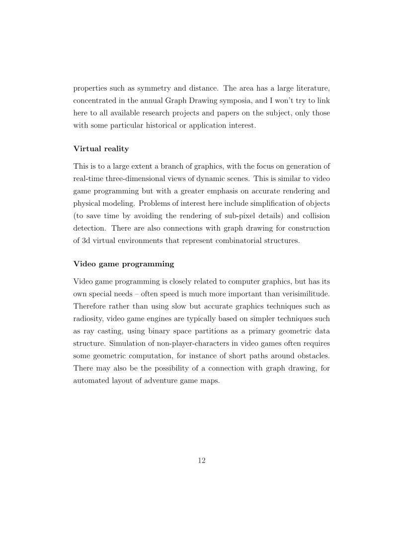
Cornered convex polygon

A cornered convex polygon P inside a circle Q is a convex polygon which is

positioned completely on one side of a diameter of Q.

Centered Convex Polygon

A convex polygon P inside a circle Q is called centered if it contains the

center of Q. See Figure 2.1(b). See Figure 2.1(a). If the center of Q is on

the perimeter of P , we still call P as a centered polygon.

21

(b)(a)

Figure 2.1: (a) Cornered Convex Polygon (b) Centered Convex Polygon.

Cutting sequence

A cutting sequence is a sequence of cuts such that after the last cut in the

sequence we have P = Q. In this thesis we consider the problem of cutting P

out of Q by line cuts with total cutting cost as small as possible. See Figure

1(b).

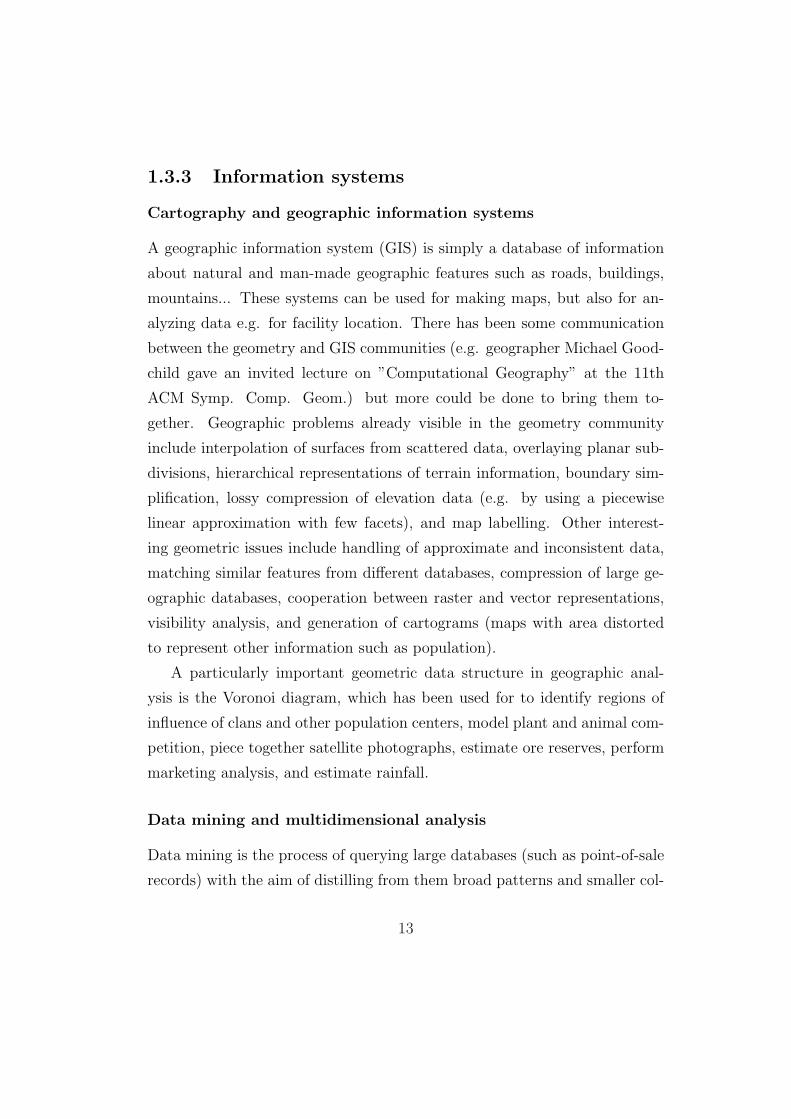
Line Cut

line cut is a line that does not run through the polygon P and divides Q into

two pieces. After a cut is made, Q is updated to the piece containing P .

l4

l1 l2

Q

P

Q

P

l3

Figure 2.2: (a) l1 and l2 are line cuts, (b)l3 and l4 are not line cuts

22

Ray cut

A cut is a ray cut if starts from a point on the perimeter of a polygon or a

circle and can or can not be ended at a point inside that polygon or circle.

Figure 2.3: Ray cut

Cut and uncut edges

The edges of P through which an edge cut has passed are called to be cut

edges of P and other edges of P are called to be uncut edges of P.

Visible edge

An edge e of P is visible from c if for every point p of e the line segment cp

does not intersect P in any other point.c is the center of Q.

2.2 Preliminaries on searching center of sphere

and ellipsoid

2.2.1 Definition

In this subsection we will give some definitions related to sphere and ellipsoid.

23

Great Circle

The circle which has the same center and diameter as a sphere is called

the great circle of that sphere. The plane with having a great circle as its

boundary is called great circular plane.

Axis Diameter

The diameter of a sphere which goes through the center of a circular plane

produced by a cross-section of that sphere and perpendicular to it, is called

the Axis Diameter of that sphere for that particular circular plane. In fig:8

Figure 2.4: Axis Diameter

ABC is a circular plane produced by a cross-section to the sphere S. PQ is a

diameter of S which goes through the center of the circular plane ABC and

perpendicular to it. As a result, PQ is the axis-diameter of the sphere S for

the circular plane ABC.

Perpendicular Great Circular Plane

In the same sphere, if G is a great circular plane which is perpendicular to a

circular plane, P produced by a cross-section of that sphere, G is called the

perpendicular great circular plane of P.

24

2.3 Preliminaries on Algorithms

We will give some important terminologies used widely in algorithms.

2.3.1 Definition

In this subsection we give some preliminaries on algorithms.

NP-Complete Problem

In computational complexity theory, the complexity class NP-complete (ab-

breviated NP-C or NPC, NP standing for Nondeterministic Polynomial time)

is a class of problems having two properties:

• Any given solution to the problem can be verified quickly (in polynomial

time); the set of problems with this property is called NP.

• If the problem can be solved quickly (in polynomial time), then so can

every problem in NP.

Although any given solution to such a problem can be verified quickly, there

is no known efficient way to locate a solution in the first place; indeed, the

most notable characteristic of NP-complete problems is that no fast solution

to them is known. That is, the time required to solve the problem using any

currently known algorithm increases very quickly as the size of the problem

grows.As a result, the time required to solve even moderately large versions

of many of these problems easily reaches into the billions or trillions of years,

using any amount of computing power available today. As a consequence,

determining whether or not it is possible to solve these problems quickly is

one of the principal unsolved problems in computer science today.

25

NP-Hard Problem

NP-hard (nondeterministic polynomial-time hard), in computational com-

plexity theory, is a class of problems informally “at least as hard as the

hardest problems in NP.” A problem H is NP-hard if and only if there is an

NP-complete problem L that is polynomial time Turing-reducible to H, i.e.

L 6T H. In other words, L can be solved in polynomial time by an oracle

machine with an oracle for H. Informally we can think of an algorithm that

can call such an oracle machine as subroutine for solving H, and solves L

in polynomial time if the subroutine call takes only one step to compute.

NP-hard problems may be of any type: decision problems, search problems,

optimization problems.

Optimization Problem

A computational problem in which the object is to find the best of all possible

solutions. More formally, find a solution in the feasible region which has the

minimum (or maximum) value of the objective function.

Optimal Solution

A solution to an optimization problem which minimizes (or maximizes) the

objective function.

Approximation Algorithm

An algorithm to solve an optimization problem that runs in polynomial time

in the length of the input and outputs a solution that is guaranteed to be

close to the optimal solution. ”Close” has some well-defined sense called the

performance guarantee.

26

Approximation Ratio

It is the ratio between the approximation result and the optimal solution

of an optimization problem. If the approximation result of an optimization

problem is C and optimal solution to that problem is C∗, then the approxi-

mation ratio is,

a = C/C∗

Constant Factor Approximation Algorithm

The approximation ratio of a constant factor algorithm is constant.

An approximation algorithm is called a c-approximation algorithm for

some constant c if it can be proven that the solution that the algorithm finds

is at most c times worse than the optimal solution. Here, c is called the

approximation ratio. For example, the vertex cover problem and travelling

salesman problem with triangle inequality each have simple 2-approximation

algorithms. In contrast to that it’s proven that the travelling salesman prob-

lem with arbitrary edge-lengths can not be approximated with approximation

ratio bounded by a constant as long as the Hamiltonian-path problem can

not be solved in polynomial time.

Polynomial Time Approximation Scheme(PTAS)

A Polynomial time approximation scheme (abbrebiated PTAS) is an algo-

rithm which takes an instance of an optimization problem and a parameter

ε > 0 and, in polynomial time, produces a solution that is within a factor εof

being optimal. For example, for the Euclidean travelling salesman problem,

a PTAS would produce a tour with length at most (1 + ε)L, with L being

the length of the shortest tour.

27

Chapter 3

Previous Works

In this chapter we will briefly discuss about some of the previous works related

to our research topics which motivated us to carry on our research interests.

In the first section, we will discuss about the previous works behind polygon

cutting and in the subsequent section, we will discuss the previous works in

the field of the geometry to find out the center of some geometric shapes like

circle, ellipse etc.

3.1 Previous Works on Polygon Cutting

Overmars et.al were the first to introduce this problem in 1985. In [13]

Overmars et.al. considered the following problem:

Given a polygonal piece of paper Q with a polygon P drawn on

it, cut P out of the piece of paper in the cheapest possible way.

They define the cut as line cut and the cost of the cut is the length of the

intersection of the cutline with the piece of paper.They asked for the cutting

sequence such that the total cost is minimum and defined this sequence as

the optimal cutting sequence. They showed in their paper that when P is

28

convex and the piece paper is convex then there does exist a finite optimal

cutting sequence. They showed the existence of a finite optimal cutting

sequence with O(n) cuts, all touching P .But in the case the piece of paper is

not convex the problem seems much harder.When only edge cuts are allowed

Overmars and Welzl proved an optimal cutting sequence can be computed

in O(m + n3) time by a simple dynamic programming algorithm.

The problem seems to be more difficult if the cuts are more general, i.e.,

they are not restricted to touch only the edges of P . In that case Bhaduri

and Chandrasekaran showed that the problem has optimal solutions that

lie in the algebraic extension of the input data field [3] and due to this

algebraic nature of this problem, an approximation scheme is the best that

one can achieve [3]. They also gave an approximation scheme [3] with

pseudo-polynomial running time.

After the indication of Bhaduri and Chandrasekaran [3] on the hardness of

the problem several researchers have given polynomial time approximation al-

gorithms for this problem. Dumitrescu proposed an O(log n)-approximation

algorithm with O(mn + n log n) running time [10, 11]. Then Daescu and

Luo [8] gave the first constant factor approximation algorithm for this prob-

lem. Their algorithm has a running time of O(n3 + (n + m) log (n + m)).

The best known constant factor approximation algorithm is due to Tan

with an approximation ratio of 7.9 and running time of O(n3 + m) [16].

In the same paper [16], he also proposed an O(log n)-approximation algo-

rithm with improved running time of O(n + m). As the best known result

so far, very recently, Bereg, Daescu and Jiang gave a simple O(m + n6

ε12)-

time (1 + ε)-approximation algorithm for this problem [2]. This problem has

also been studied when Q is a non-convex polygon [13], P is a non-convex

polygon [7, 8, 16], and/or the cuts are ray cuts [7, 8, 16].

29

3.2 Previous Works on Searching for the Cen-

ter of a Certain Geometric Shape Under

Definite Constraints

Biedl et al. [4] first posed the question of finding the center of a circle,

starting with a point on the boundary, where the only allowed operations are

an interior and exterior query, marking a point, and computing the line or

midpoint between any two marked points. The problem was motivated by

the problem of searching a skier who is victim of an avalanche. The skiers

bear with them small radios which are known as transceivers. Transceivers

have two modes, transmitting and receiving. Whenever a skier becomes

victim of an avalanche he sets his transmitter on transmitting mode and the

rest of the skiers set their transmitter on receiving mode. Then the mission

is to find out the victim as quickly as possible because the victim cannot

survive for a long under the snow. The transceiver, in its transmitting mode,

continuously transmits signal which has a fixed range. Any transceiver in

receiving mode can detect this signal if it is inside that range. But if the

receiving transceiver goes beyond that range, the signal fades. The skiers

who try to find out the victim follow the signal and try to reach the victim

as quickly as possible. The transmitting range of the transceiver of the

victim was at first thought to be bounded by a circle with the victim at the

center of it and in the Avalanche Handbook, there was a solution for how

to reach the center of that circle to rescue that victim. Biedl et al. showed

a more efficient strategy for searching the center of a circle which is known

as right angle strategy. Later in his paper he claimed that the boundary of

the range of the transmitter can better be modelled as an ellipse and he

posed an open problem for an efficient strategy of searching the center of an

ellipse. Later Michael A. Burr [5] solved that problem with parallel chord

30

method. In both of their works they considered the searching space to be two

dimensional and did not give any clue of what to do in case of searching in

three dimensional spaces. But the avalanche actually occurs on the slides of a

hill or a mountain and the three dimensional model is much more appropriate

in these cases. Moreover helicopters are used for rescuing skiers nowadays

which can easily move in three dimensions. So, an efficient three dimensional

model for rescuing the avalanche victim is will be very much helpful and

useful. Again, if we consider a victim under water or in space, we can not

use the two dimensional model at all. So, the efficient searching technique

should handle three dimensional cases which inherently takes care of the

cases of two dimensions. Here we showed efficient strategies for searching in

three dimensional spaces in two models, first spherical and then ellipsoidal

corresponding to the circular model proposed by the Avalanche handbook

[14] and T. Beidl [4]respectively. Again, the strategy for elliptical model

was not complete as the ellipse has some dead areas where no signal can

reach. So, the elliptical model proposed by Michael A. Burr [5] does not

work perfectly in some cases due to dead areas.

Figure 3.1: Problems associated withe the two dimensional search techniques.

31

T. Beidl et al. [4] proposed the right angle strategy to find out the center

of a circle for this type of robot. His strategy was to take two consecutive

mutually perpendicular moves to reach from one endpoint to another end-

point of a diameter of the circle. The strategy is described in Figure 2. This

strategy fails to detect the center of a sphere.

Michael A. Burr [5] solved the problem of searching the center of al ellipse

using a special property of an ellipse. The property is that the line joining

the midpoints of any two parallel chords of an ellipse is a diameter of that

ellipse and the midpoint of that diameter is the center of that ellipse. For

Figure 3.2:

example in Figure 18 , According to his strategy, if the searcher starts from

the point A and advance along AB chord , reaches B, finds out the midpoint

of AB chord which is M and then goes to the point B again. Then it turns 90

degrees inside the ellipse and moves along BC chord and reaches C. Then the

searcher turns 90 degrees inside the ellipsoid again, moves along CD chord

and finds out its midpoint, N. Now from N the searcher moves along NM

and gets the PQ diameter and gets the midpoint of it which is eventually the

center of the ellipse.

32

Chapter 4

Cutting a Convex Polygon Out

of a Circle

In this thesis we first consider the problem where Q is a circle and P is convex

polygon such that P is bounded by a half circle of Q and all the cuts are line

cuts. We give a simple linear time O(log n)-approximation algorithm for this

problem where n is the number of vertices of the polygon. We also gave an

constant factor approximation algorithm for this problem. Finally, we gave

an constant factor approximation algorithm in general case i.e. cutting a

convex polygon out of a circle in which the convex polygon is not necessarily

cornered. For both of the cases we also determined the Polynomial Time

Approximation Scheme (PTAS).

4.1 The Basic Problem that We Studied

A line cut is a line that does not run through the polygon P and divides Q

into two pieces. After a cut is made, Q is updated to the piece containing P .

The cost of a cut is the length of the intersection of the cut with Q. A cutting

sequence is a sequence of cuts such that after the last cut in the sequence we

33

have P = Q. In this thesis we consider the problem of cutting P out of Q

by line cuts with total cutting cost as small as possible. See Figure 4.1(b).

P

Q

PP

(a)(b) (c)

Q Q

Figure 4.1: (a) A convex polygon. (b,c) Two different cutting sequences to

cut P out of Q. The cost of the sequence in (b) is more than that in the (c).

The problem of cutting a polygon P out of a piece of paper Q with

minimum total cutting length is a well studied problem in computational

geometry. Researchers studied several variations of the problem, such as P

and Q are convex or non-convex polygons and the cuts are line cuts or ray

cuts. Though the problem is approached considering the piece of paper is

being a convex polygon, we are the first to consider it as a circle. At first

we approach the problem in a restricted case that is the polygon P inside

the circle Q is cornered and give approximation algorithm regarding this

restricted case.Then we solved the problem in more general way where the

polygon P is not necessarily cornered.

4.2 Algorithm for Cornered Convex Polygon

In this section we shall represent the basic ideas of establishing our algo-

rithms by introducing some lemma and theorem. In the first subsection we

shall represent algorithm for the cornered convex polygon with O(log n) ap-

34

proximation ratio and O(n) runtime, in the subsequent subsection we shall

give the second algorithm which is a constant factor approximation algorithm

with approximation ratio 6.48 and running time O(n3).

Let ll′ be a chord of Q. ll′ divides Q into two circular segments, one is

bigger than a half circle and is called the bigger segment created by ll′, and

the other one is called the smaller segment created by ll′. Let tt′ be another

chord intersecting ll′ at x such that tx is in the smaller segment of ll′. See

Figure. Then the following lemma holds.

Lemma 4.2.1. Length of xt is no bigger than length of ll′.

(a) (b)

b′x

t′

l′

l

t

b c

a

b′

b′

c′c′

Figure 4.2: Some preliminaries.

Following lemma is also obvious, whose illustration can be found in Fig-

ure.

Lemma 4.2.2. Let 4abc be an obtuse triangle with ∠bac being the obtuse

angle. Consider any line segment connecting two points b′ and c′ on ab and

ac, respectively, possibly one of b′ and c′ coinciding with b or c respectively.

Then the angle ∠bb′c′ and ∠cc′b′ are obtuse.

35

4.2.1 Algorithm 1

Our algorithm has four phases : (1) D-separation, (2) triangle separation,

(3) obtuse phase and (4) curving phase. In D-separation phase, we cut out

a small portion of Q (less than the half of Q in size) which contains P (and

looks like a “D”). Then in triangle separation phase we reduce the size of

Q even more by two additional cuts and bound P by almost a triangle. In

obtuse phase we assure that all the portions of Q that are not inside P are

inside obtuse triangles. Finally, in curving phase we cut P out of Q by

cutting in rounds.

Let C∗ be the optimal cutting length of P from Q. Clearly C∗ ≥ |P |,where |P | is the length of the perimeter of P .

D-Separation

A D of the circle Q is a circular segment of Q which is smaller than an half

circle of Q. By a D-separation of P from Q we mean a line cut along a chord

of Q that creates a D containing P . In general for a circle Q and a convex

polygon P there may not exist any D-separation of P . But in our case since

P is cornered, there always exists a D-separation of P .

We will first observe that there exists only one minimum-cost D-separation

C1 of P and then we will find that C1. (For our algorithm, however, showing

the uniqueness of the minimum D-separation is not required).

Lemma 4.2.3. The minimum-cost D-separation C1 for P can be found in

O(n) time.

Proof. Clearly C1 must touch P . So, C1 must be a vertex cut or an edge cut

of P . Observe that any vertex cut or edge cut that is a D-separation must

be through a visible vertex or a visible edge. Let e be a visible edge of P .

Let ll′ be a line cut through e. Let cp be the line segment perpendicular to

ll′ at p. If p is a point on e, then we call e a critical edge of P and ll′ a

36

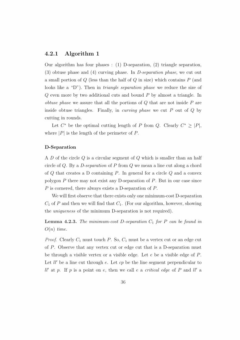
critical edge cut of P . Observe that since P is convex, it can have at most

one critical edge. Similarly, let v be a vertex of P . Let tt′ be a vertex cut

through v. Let cp be the line segment perpendicular to tt′ at p. If tt′ is such

that p = v, then we call v a critical vertex of P and tt′ a critical vertex cut

of P . Again observe that P can have at most one critical vertex. Moreover,

P has a critical edge if and only if it does not have a critical vertex. See

Figure 4.3. Now, if P has the critical edge e, then C1 is the corresponding

critical edge cut ll′. C1 is minimum, because any other vertex cut or edge cut

of P is either closer to c (and thus bigger) or does not separate c from P . On

the other hand, if P has the critical vertex v, then C1 is the corresponding

critical vertex cut tt′ of P . Again, C1 is minimum by the same reason.

For the running time note that all visible vertices and visible edges of P

can be found in linear time. Then finding whether an edge of P is critical

takes constant time. Over all edges finding the critical edge, if it exists, takes

O(n) time. Similarly, for each visible vertex v we can check in constant time

whether v is critical or not by comparing the angles of cv with two adjacent

edges of v, which takes constant time. Over all visible vertices, it takes linear

time.

t′

c

Q

Pe

c

Q

Pv

l

l′

t

Figure 4.3: Critical edge and critical vertex.

37

Lemma 4.2.4. Cost of C1 is at most C∗.

Proof. Consider any optimal cutting sequence C. C must separate P from

c. However, it may do that by using a single cut or by using more than

one cut. If it uses a single cut, then it is in fact doing a D-separation. By

Lemma 4.3.5, it can not do better than C1, and therefore, cost of C1 is at

most C∗.

Now we assume that C separates P from c by more than one cut. There

are several cases here. We will prove that in any case the cutting cost of

separating P from c is even higher than that for a single cut. Let C be the

first cut in C that separates c from P . C can not be the very first cut of

C, otherwise, we are in the previous case considered above. It implies that

C smaller than a chord of Q. See Figure 2.2. Let a and a′ be the two end

points of C. Let bb′ be the chord of Q that contains aa′ where b is closer to

a than to a′. Now, at least one of a and a′ is not incident on the boundary

of Q. We first assume that a is not incident to the boundary of Q but a′ is.

Let Cx = xx′ be the cut that was applied before C and intersects C at a.

Since Cx does not separate c from P , the bigger segment of Cx contains P ,

c and a. Now if x′ is an end point of Cx, then by Lemma 4.2.1 ab is smaller

than xx′. It implies that having Cx in addition to C1 increases the cost of

separating P from c (see Figure 2.2(a)). Similarly, if x′ is not an end point

of Cx, and thus another cut is involved, then by Lemma 4.2.1 the cost will

be even more (see Figure 2.2(b)).

Now consider the case when both a and a′ are not incident on Q. So

at least two cuts are required to separate ab and a′b′ from bb′. Let those

two cuts be Cx and Cy respectively. Let xx′ and yy′ be the two chords of

Q along which Cx and Cy are applied. Now if Cx and Cy do not intersect,

then by applying the above argument for each of them we can say that the

cutting cost is no better than that for a single cut. But handling the case

when Cx and Cy intersect is not obvious. (See Figure 2.2(c,d)). Let z′ be

38

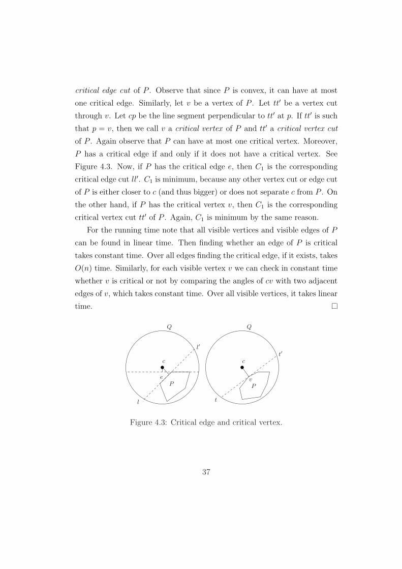
their intersection point. Again there may be several subcases: x and y may

or may not be end points of Cx and Cy. Assume that both x and y are end

points of Cx and Cy. Remember that none of Cx and Cy separates P from

c. So region bounded by xz′y must contain P and c inside of it and in that

case the total length of xz′ and yz′ is at least the diameter of Q, which is

bigger than bb′ (see Figure 2.2(c)). For the other cases, where at least one of

x and y is not an end point of Cx and Cy, it can be recursively proven that

the cost is even more (For example, see Figure 2.2(d)).

(c) (d)(b)(a)

a′ = b′ a′ = b′

c

bx

c

bx

x′

b′

bx

y

z′

c

b′

bx

y

z′

c

x′

y′x′ x′

y′

a

a′

a a

a′

a

Figure 4.4: Separating P from c by using more than one cut increases the

cutting cost. The cutting length is shown in bold lines.

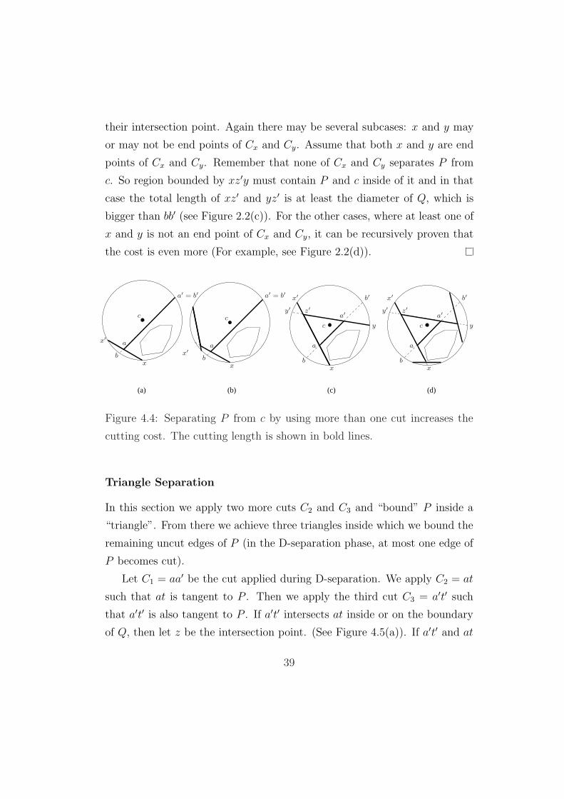
Triangle Separation

In this section we apply two more cuts C2 and C3 and “bound” P inside a

“triangle”. From there we achieve three triangles inside which we bound the

remaining uncut edges of P (in the D-separation phase, at most one edge of

P becomes cut).

Let C1 = aa′ be the cut applied during D-separation. We apply C2 = at

such that at is tangent to P . Then we apply the third cut C3 = a′t′ such

that a′t′ is also tangent to P . If a′t′ intersects at inside or on the boundary

of Q, then let z be the intersection point. (See Figure 4.5(a)). If a′t′ and at

39

do not intersect, then let z be the intersection point of the lines containing

at and a′t′. (See Figure 4.5(b)).

We get three resulting triangles Ta, Ta′ , Tz having a, a′ and z, respectively,

as a vertex as follows. We describe only Ta, description of Ta′ , Tz are analo-

gous. If C1 is an edge cut, then let rr′ be the corresponding edge such that

a is closer to r than to r′. (See Figure 4.5(a)). If C1 is a vertex cut, then let

r be the corresponding vertex of P . Let s be the similar vertex due to C2.

(See Figure 4.5(b)). Then Ta = 4ars. The polygonal chain of P bounded by

this triangle is the edges from r to s that reside inside Ta.

r

a′

a

r

s

zt

t′

(a) (b)

a′

a

z

s

t′

t

r′

Figure 4.5: Triangle separation.

Lemma 4.2.5. Total cost of C2 and C3 to achieve Ta, Ta′ and Tz is at most

2C∗. Moreover, C2 and C3 can be found in linear time.

Proof. Whether z is within Q or outside Q, the length of at and a′t′ can not

be more than twice the length of aa′, which, by Lemma 4.3.5, is no more

40

than C∗. So the total cost of C2 and C3 is at most 2C∗.

To find at linearly, we can simply scan the boundary of P starting from

the vertex or edge where aa′ touches P and check in constant time whether

a tangent of P is possible through that vertex or edge. Similarly we can find

a′t′ within the same time.

Obtuse Phase

Consider the triangle Ta obtained in the previous section. We call the vertex

a of Ta the peak of Ta and the edge rs the base of Ta. Let the polygonal

chain of P that is bounded by Ta be Hrs. Observe that the angle of Ta at a

is acute. Similarly, the angle of Ta′ at its peak a′ is also acute. However, the

angle of Tz at its peak z may be acute or obtuse.

We obtain, by applying a cut, for each of Ta, Ta′ and Tz (if Tz is acute)

one or two triangles such that the angle at their peaks are obtuse and they

combinely bound the polygonal chain of the corresponding triangle. We

describe the construction of the triangle(s) from Ta only, description for the

triangles obtained from Ta′ and Tz are analogous.

Let Pa be the polygonal chain bounded by Ta. Length of ar and as may

not be equal. W.l.o.g. assume that as is not larger than ar. Let s′ be the

point on ar such that length of as′ equals to the length of as. Connect ss′

if s′ is different from r. We will find a line segment inside Ta such that it

is tangent to Pa and is parallel to ss′. We have two cases: (i) ss′ itself is a

tangent to Pa, and (ii) ss′ itself is a tangent to Pa. Case (i): If ss′ itself is

tangent to Pa (at s), we apply our cut along ss′. This may be a vertex cut

through s. In that case we get the resulting obtuse triangle 4rss′ and the

polygonal chain bounded by this triangle is same as Pa. (See Figure 4.6(a)).

On the other hand, this may be an edge cut through the edge of Pa that is

incident to s. Let u be the vertex other than s of the edge of the edge cut.

Then our resulting obtuse triangle is 4rus′ and the polygonal chain bounded

41

by this triangle is the edges from r to u. (See Figure 4.6(b)). Case(ii): For

this case, let u, u′ be two points on as and ar, respectively, such that uu′ is

tangent of Pa and is parallel to ss′. We apply the cut along uu′. Again this

cut may be a vertex cut or an edge cut. If it is a vertex cut, let g be the

vertex of the cut. Then we get two obtuse triangles 4ru′g and 4sug and

the polygonal chains bounded by them are the sets of edges from r to g and

from g to s respectively. (See Figure 4.6(c)). If it is an edge cut, then let

gg′ be the edge of the edge cut with u being closer to g than to g′. Then

we get two obtuse 4ru′g′ and 4sug and the polygonal chains bounded by

them are the sets of edges from r to g′ and from g to s respectively. (See

Figure 4.6(d)).

(d)(a) (b) (c)

a

r

ss′

u′ ug

a

r

ss′

a

r

ss′ u

a

r

ss′

u′ ugg′

Lemma 4.2.6. Total cost of obtaining obtuse triangles from Ta, Ta′, and Tz

is at most C∗. Moreover, they can be found in O(log n) time.

Proof. Consider the construction of the obtuse triangle(s) from Ta. Length

of the cut ss′ or uu′ is at most the length of their base ss′, which is bounded

by the length of Pa. Over all three triangles Ta, Ta′ and Tz, the total cutting

length is bounded by the length of the perimeter of P . Since C∗ is at least

the length of the perimeter of P , the first part of the lemma holds.

42

(d)(c)

a

r

ss′

u′ ug

a

r

ss′

u′ ugg′

Figure 4.6: Obtaining obtuse triangle(s) from Ta.

For running time, in Ta, we can find the tangent of Pa in O(log |Pa|) time

by using a binary search. Over all three triangles Ta, Ta′ and Tz, we need a

total of O(log n) time.

Curving Phase

After the obtuse phase the edges of P that are not yet cut are partitioned

and bounded into polygonal chains with at most six obtuse triangles. In this

section we apply the cuts in rounds until all edges of P are cut. Our cutting

procedure is same for all obtuse triangles and we describe for only one.

Let Tu = 4gus with peak u and base gs be an obtuse triangle. See

Figure 4.7. Let the polygonal chain bounded by Tu be Pu. Let the edges of

Pu be e1, . . . , ek with k ≥ 2. We will apply cuts in rounds and all cuts are

edge cuts. In the first round we apply an edge cut C ′ along the edge ek/2.

Then we connect g and s with the two end points of ek/2 to get two disjoint

triangles. Since Tu is obtuse, by Lemma 4.2.2 these two new triangles are

also obtuse. So, as a result we cut out one polygonal edge and get two new

obtuse triangles. In the next round we work on each of these two triangles

43

recursively, then in the next next round we work on four triangles and so on.

We continue in this way until all edges of Pu are cut.

sg

u

Figure 4.7: Curving phase

Lemma 4.2.7. There are at most O(log k) rounds of cuts to cut all edges

of Pu. Moreover, the total cost of these cuts is |Pu| log k, where |Pu| is the

length of Pu, and the total running time is O(|Pu|).

Proof. At each round the number of triangles get doubled and the number

of edges that become cut also get doubled. So after log k rounds all k edges

are cut.

At each round the total length of the bases plus the length of the edges

that are being cut is no more than |Pu|. So, the total cutting cost is |Pu| log k

over all rounds.

For running time, for applying an edge cut we always move to the middle

edge of a polygonal chain. So, finding an edge cut takes constant time.

Moreover, after each cut the corresponding edge is never considered again.

So, over all rounds we can have at most |Pu| cuts, which gives a running time

of O(|Pu|).

Corollary 4.2.8. The total cost of curving phase is C∗ log n and the running

time is O(n).

44

Combining the results of all four phases, we get the following theorem.

Theorem 4.2.9. Given a circle Q and a cornered convex polygon P of n

edges within Q, P can be cut out of Q by using line cuts in O(n) time with

a cutting cost of O(log n) times the optimal cutting cost.

4.2.2 Algorithm 2

In this section we shall present our second algorithm which cuts P out of Q

with a constant approximation ratio of 6.48 and running time of O(n3). This

algorithm has three phases: (1) D-separation, (2) cutting out a minimum

area rectangle that bounds P and (3) cutting P out of that rectangle by only

edge cuts. The D-separation phase is same as that of our first algorithm and

we assume that this phase has been applied.

Cutting a Minimum Area Bounding Rectangle

We will use the technique of rotating calipers, which is a well known concept

in computational geometry and was first introduced by Toussaint [ref]. We

use the method described by Toussaint [ref].

A pair rotating calipers remain in parallel. It rotate along the boundary

of an object with two calipers being tangents to the object. If the object is

a convex polygon P , then one fixed caliper, which we call the base caliper,

is tangent along an edge e of P and the other caliper is tangent to a vertex

or an edge of P . In the next step of the rotation, the base caliper moves to

the next edge adjacent to e and continue. The rotation is complete when the

base caliper has encountered all edges of P .

For our case we use two pairs of rotating calipers, where one pair is

orthogonal to the other. We fixed only one caliper, among the four, as the

base caliper. As we rotate along the boundary of P , we always place the base

caliper along an edge of P and adjust other three calipers as the tangents of

45

P . The four calipers give us a bounding rectangle of P . After the rotation

is complete, we identify the minimum area rectangle among the n bounding

rectangles. For that rectangle we apply one cut along each of its edges that

are not collinear with the chord of the D.

The above technique can be done in O(n) time [ref]. Once the base

calipers is placed along an edge, the other three calipers are also rotated and

adjusted to make them tangent to P . Notice that each caliper “traverses”

an edge or a vertex exactly once.

fig here

Lemma 4.2.10. The cost of cutting a minimum area rectangle out of the D

achieved from the D-separation phase is no more than 2.57C∗.

Proof. There can be at most four pieces, other than the one inside the bound-

ing rectangle, resulting from four cuts applied to the D. The length of each

cut is no more than the portion of the perimeter of D that is separated by

that cut. So, as a whole the total cutting cost is no more than the perimeter

of D. Also see ref[fig].

Now the perimeter of D is CD +RΘ, where CD is the length of the chord

of D and Θ is the angle made by the arc of D at the center c. Since CD

is the cost of D-separation, which by ref[lemma] is bounded by C∗,Θ is at

most Π, and C∗ can not be more than 2R, the maximum perimeter of D is

C∗ + (C∗/2)Π = 2.57C∗.

Cutting P out of a Minimum Area Rectangle by Only Edge Cuts

For this phase we simply apply the constant factor approximation algorithm

of Tan [ref]. If P is bounded by a minimum area rectangle, then Tans

algorithm cuts P out of the rectangle by using only edge cuts in O(n3) time

and with approximation ratio (1.5 +√

(2)) [ref]. We summerize the result of

our second algorithm in the following theorem.

46

Theorem 4.2.11. Given a circle Q and a cornered convex polygon P of n

edges within Q, P can be cut out of Q by using line cuts in O(n3) time with

a cutting cost of 6.48 times the optimal cutting cost.

Proof. We have the cutting cost of C∗ for D-Separation, 2.57C∗ for cutting

the minimum area rectangle, and (1.5 +√

(2))C∗ for cutting P out of the

rectangle, which give a total cost of 6.48C∗.

4.3 Algorithms for General Case

In this section, we consider the problem where Q is a circle and P is a con-

vex polygon which may or may not be cornered. We give three algorithms

for this problem. Our first algorithm runs in O(n) time and has an approx-

imation ratio of O(log n). Next, we give a constant factor approximation

algorithm having approximation ratio of 6.74 and 7.9-constant factor when

P is cornered or not respectively, and runs in O(n3) time. Finally, we give a

polynomial time approximation scheme (PTAS) which has an approximation

ration of (1 + ε) and runs in O( n6

ε12) time.

In this thesis we denote the radius of Q by R, diameter of P by D, the

boundary of P (resp. Q) by ∂P (resp. ∂Q) and length of the perimeter of

P (resp. Q) by |P |(resp. |Q|). We denote an optimal cutting cost of P out of

Q as C∗. Let Q′ denote the minimum rectangle containing P . Let Dx (resp.

Dy) denote the x− distance (resp. y− distance) between two vertical (resp.

horizontal) edges of Q′. Then, Dx = D, Dy = D,and Dx + Dy =√|S ∗ |/2

hold.

The following two lemmas are obvious:

Lemma 4.3.1. C∗ ≥ |P |.

Lemma 4.3.2. C∗ ≥ 2D.

47

Now we prove an important lemma which would be necessary to compute

the approximation ratio later in this thesis.

Lemma 4.3.3. If P is a centered convex polygon, C∗ ≥ 2R.

z

c a d

b

x

y

m

n

l

P

Figure 4.8: Lower bound for C∗.

Proof. by Lemma 4.3.1, C∗ ≥ |P |.Observe that, any cutting sequence that

separate P from Q and has two disjoint subsequences each start from a point

of Q and ends at a point of P . Let a and m are two such points of P and

b and n are the two corresponding points on Q respectively. See Figure 4.9.

Now, |ac| + |ab| ≥ R, and |cm| + |mn| ≥ R. Again, |ac| + |cm| ≤ |P |. So,

the total cutting cost is at least |P |+ |mn|+ |ab| ≥ 2R. Hence proved.

For a vertex v of P , we define the chord through v as the intersect-

ing segment of Q with a line through v. Let Cv denote a shortest chord

through a vertex v of P . Let V (P ) be the set of vertices of P , and let

|C| = maxv∈V (P )|Cv|. Then, |C| ≤ |C∗| holds [10]. A chord through

v ∈ V (P ) is called an ST − chord if it is a shortest chord through v and

tangent to P . We denote it by STv.Let |ST | = minv∈V (P )|STv|.Now the following lemma is obvious.

48

Lemma 4.3.4. The ST − chord can be found in O(n) time.

P

Figure 4.9: shortest chord through a point inside a circle is perpendicular o

the line joining the center and that point.

4.3.1 Separating Minimum Rectangle Bounding P Us-

ing Rotating Calipers

Almost all of our algorithms cuts a minimum rectangle bounding P at the

first step. We choose the rotating calipers technique for determining this

rectangle. This technique was introduced by G.Toussaint in [17]. Chan-

drasekaran et. al. used this approach in [7] but in a different way so that

their algorithm becomes dependent on the number of edges of Q. But we

used it in such a way so that the running time is only dependant on n. We

discuss the technique here.

In [17], G. Toussaint proved that the rectangle of minimum area enclosing

a convex polygon has a side collinear with one of the edges of the polygon.

This theorem can be deployed to determine the minimum area rectangle

bounding P . For cutting out the minimum area rectangle , we use two pairs

of orthogonal rotating calipers as the method described by G. Toussaint [17]

in O(n) time. This process involves rotating two orthogonal pairs of calipers

49

around P keeping one side of one calipers always collinear with one of the

edges of P . Hence, we get a minimum area rectangle around P .

=⇒P

Figure 4.10: (a) Rotating Calipers (b) Rotating two orthogonal pairs of

rotating calipers.

Lemma 4.3.5. The cost of cutting out minimum area rectangle bounding P

is no more that 2√

2C∗ where P is centered.

2Ra

a

a

a

Figure 4.11: Upper bound of the cut length of minimum area rectangle

bounding P when P is centered.

Proof. We know that the maximum rectangle enclosed in a circle is a square

whose diagonal is 2R. See Figure 4.11. Let us assume that the side of the

50

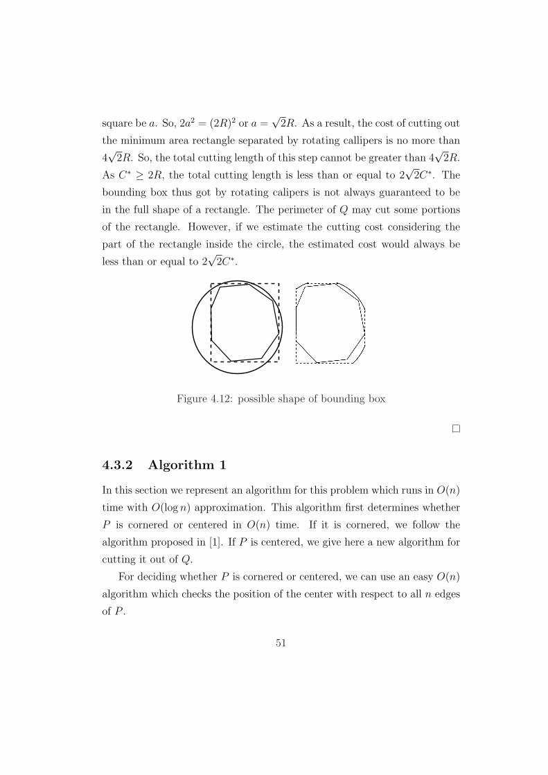
square be a. So, 2a2 = (2R)2 or a =√

2R. As a result, the cost of cutting out

the minimum area rectangle separated by rotating callipers is no more than

4√

2R. So, the total cutting length of this step cannot be greater than 4√

2R.

As C∗ ≥ 2R, the total cutting length is less than or equal to 2√

2C∗. The

bounding box thus got by rotating calipers is not always guaranteed to be

in the full shape of a rectangle. The perimeter of Q may cut some portions

of the rectangle. However, if we estimate the cutting cost considering the

part of the rectangle inside the circle, the estimated cost would always be

less than or equal to 2√

2C∗.

Figure 4.12: possible shape of bounding box

4.3.2 Algorithm 1

In this section we represent an algorithm for this problem which runs in O(n)

time with O(log n) approximation. This algorithm first determines whether

P is cornered or centered in O(n) time. If it is cornered, we follow the

algorithm proposed in [1]. If P is centered, we give here a new algorithm for

cutting it out of Q.

For deciding whether P is cornered or centered, we can use an easy O(n)

algorithm which checks the position of the center with respect to all n edges

of P .

51

If P is cornered then Ahmed et. al gave an algorithm in [1] to cut P out

of Q in O(n) running time and O(log n) approximation ratio. We follow the

same algorithm here. The algorithm has four phases : (1) D-separation, (2)

triangle separation, (3) obtuse phase and (4) curving phase. In D-separation

phase, a small portion of Q (less than the half of Q in size) which contains P

(and looks like a “D”) is cut out. Then in triangle separation phase the size

of Q is reduced even more by two additional cuts and bounds P by almost

a triangle. In obtuse phase, it is assured that all the portions of Q that are

not inside P are inside obtuse triangles. Finally, in curving phase P is cut

out of Q by cutting in rounds.

If P is centered we cut P out of Q in two steps: (1) cutting out a minimum

area rectangle containing P and (2) cutting P out of that rectangle.

For cutting out minimum area rectangle, we use the rotating calipers

technique described in Section 4.3.1. As a result the separation phase runs

in O(n) time and the cut length is less than or equal to 2√

2C∗.

After that we cut P out of the minimum area rectangle by cutting in

rounds in the similar way described in the curving phase of the [1]. We do

not need the obtuse phase here , as all the angles of the rectangle are right

angles. Hence, the curving phase will run in O(n) time and will have an

approximation ration of O(log n).

So, the following theorem holds.

Theorem 4.3.6. Algorithm 1 cuts P out of Q in O(n) time with O(log n)

approximation ratio.

4.3.3 Algorithm 2

In this section we represent an algorithm with constant factor approxima-

tion ratio and O(n3) running time. The constant factor is 6.74 or 7.9 if P

is centered or cornered respectively. This algorithm actually modifies the

52

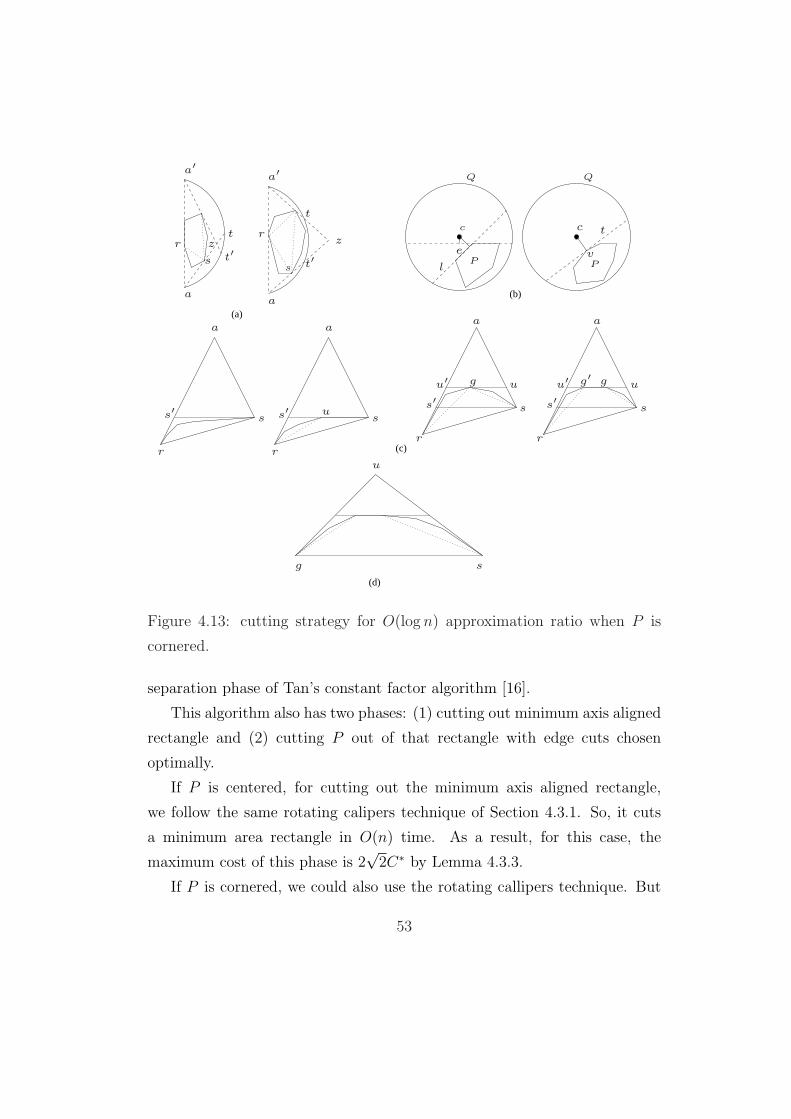
(a)

(b)

(d)

(c)

s

a

r

s

zt

t′

a′

a

r

ss′

a

r

ss′ u

a

r

ss′u′ ugg′

a′

a

zr

s

t

t′

c

Q

Pe

l

c

Q

P

t

v

a

r

ss′u′ ug

g

u

Figure 4.13: cutting strategy for O(log n) approximation ratio when P is

cornered.

separation phase of Tan’s constant factor algorithm [16].

This algorithm also has two phases: (1) cutting out minimum axis aligned

rectangle and (2) cutting P out of that rectangle with edge cuts chosen

optimally.

If P is centered, for cutting out the minimum axis aligned rectangle,

we follow the same rotating calipers technique of Section 4.3.1. So, it cuts

a minimum area rectangle in O(n) time. As a result, for this case, the

maximum cost of this phase is 2√

2C∗ by Lemma 4.3.3.

If P is cornered, we could also use the rotating callipers technique. But

53

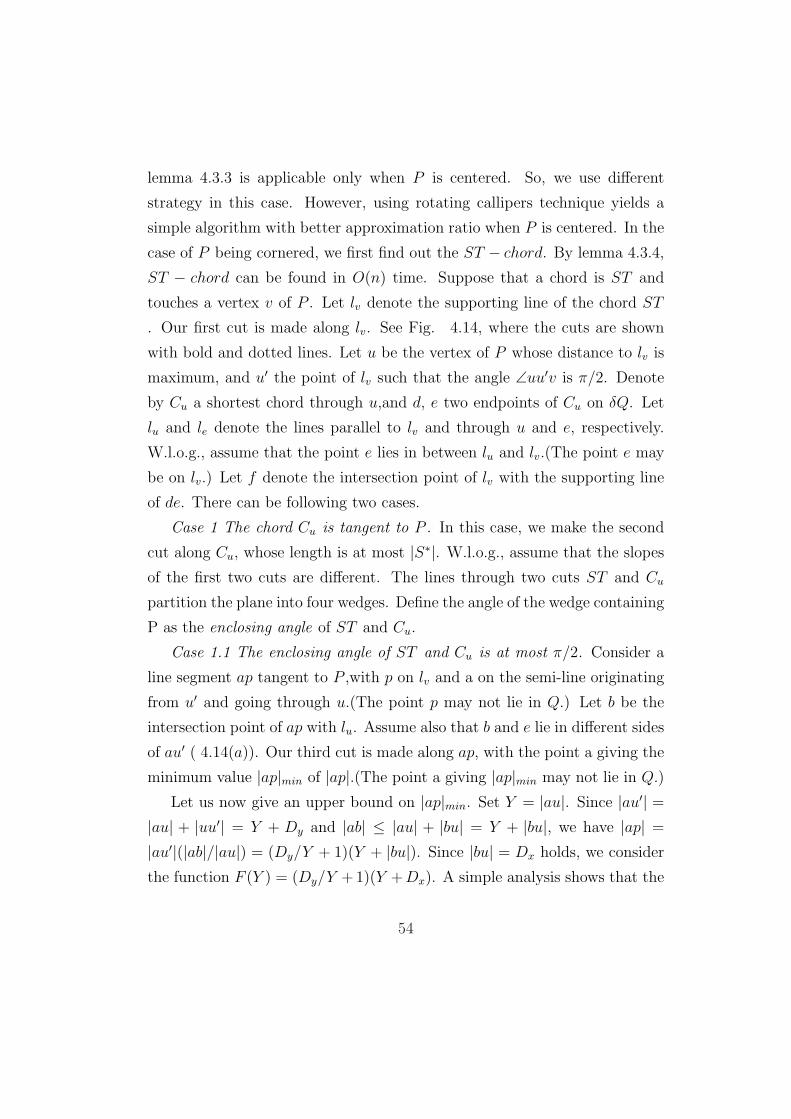
lemma 4.3.3 is applicable only when P is centered. So, we use different

strategy in this case. However, using rotating callipers technique yields a

simple algorithm with better approximation ratio when P is centered. In the

case of P being cornered, we first find out the ST − chord. By lemma 4.3.4,

ST − chord can be found in O(n) time. Suppose that a chord is ST and

touches a vertex v of P . Let lv denote the supporting line of the chord ST

. Our first cut is made along lv. See Fig. 4.14, where the cuts are shown

with bold and dotted lines. Let u be the vertex of P whose distance to lv is

maximum, and u′ the point of lv such that the angle ∠uu′v is π/2. Denote

by Cu a shortest chord through u,and d, e two endpoints of Cu on δQ. Let

lu and le denote the lines parallel to lv and through u and e, respectively.

W.l.o.g., assume that the point e lies in between lu and lv.(The point e may

be on lv.) Let f denote the intersection point of lv with the supporting line

of de. There can be following two cases.

Case 1 The chord Cu is tangent to P . In this case, we make the second

cut along Cu, whose length is at most |S∗|. W.l.o.g., assume that the slopes

of the first two cuts are different. The lines through two cuts ST and Cu

partition the plane into four wedges. Define the angle of the wedge containing

P as the enclosing angle of ST and Cu.

Case 1.1 The enclosing angle of ST and Cu is at most π/2. Consider a

line segment ap tangent to P ,with p on lv and a on the semi-line originating

from u′ and going through u.(The point p may not lie in Q.) Let b be the

intersection point of ap with lu. Assume also that b and e lie in different sides

of au′ ( 4.14(a)). Our third cut is made along ap, with the point a giving the

minimum value |ap|min of |ap|.(The point a giving |ap|min may not lie in Q.)

Let us now give an upper bound on |ap|min. Set Y = |au|. Since |au′| =|au| + |uu′| = Y + Dy and |ab| ≤ |au| + |bu| = Y + |bu|, we have |ap| =

|au′|(|ab|/|au|) = (Dy/Y + 1)(Y + |bu|). Since |bu| = Dx holds, we consider

the function F (Y ) = (Dy/Y +1)(Y +Dx). A simple analysis shows that the

54

(a) (b) (c)

(d)(e) (f)s

P

u

lv

lu

v

p

p v f u′

e

P

le p

a

lv

le

lu

p

v

g

dQ

lu

f

e

d

P

Q

lu

e

g b

d

a

i

c Pe

u

P

p

c u

a

d

Q

u

b

u′

lv

Q

a

b u

d

lu

d d′

lub = u

Q

c c′

lv v

h

b c

e lv

c

Q

lv v f

P

g b u

Figure 4.14: cutting out minimum area rectangle with constant cut length.t

minimum value F (Y )min of F (Y ) is achieved when Y =√

DxDy. Hence,

F (Y )min < (Dy/√

DxDy + 1)(√

DxDy + Dx) ≤ (1 +√

2/2)|S∗|.It is clear that |ap|min = F (Y )min. Thus, the length of the cut along ap

is less than (1 +√

2/2)|S∗|. Finally, we make a cut along lu, and two cuts

parallel to au’ and tangent to P . This results in the minimum rectangle Q′

containing P (only part of Q′ may result). See Fig. 4.14(b). The sum of the

cost taken for the cut along the chord ST and the costs for the last three cuts

is less than |Q′|+ |ST | − |T |. Since |ST | = |T |, we have |Q′|+ |ST | − |T | ≤√

2(|P |+ |ST | − |T |) <√

2|S∗|. Hence, the total cost of these six cuts is less

than (2 + 3√

2)|S∗|.Case 1.2 The enclosing angle of ST and Cu is larger than π/2 ( 4.14(b)).

Consider a line segment ap tangent to P , with the point p on lv and the

55

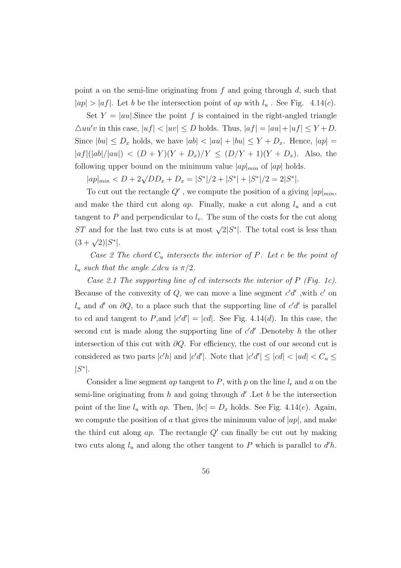
point a on the semi-line originating from f and going through d, such that

|ap| > |af |. Let b be the intersection point of ap with lu . See Fig. 4.14(c).

Set Y = |au|.Since the point f is contained in the right-angled triangle

4uu′v in this case, |uf | < |uv| ≤ D holds. Thus, |af | = |au|+ |uf | ≤ Y +D.

Since |bu| ≤ Dx holds, we have |ab| < |au| + |bu| ≤ Y + Dx. Hence, |ap| =

|af |(|ab|/|au|) < (D + Y )(Y + Dx)/Y ≤ (D/Y + 1)(Y + Dx). Also, the

following upper bound on the minimum value |ap|min of |ap| holds.

|ap|min < D + 2√

DDx + Dx = |S∗|/2 + |S∗|+ |S∗|/2 = 2|S∗|.To cut out the rectangle Q′ , we compute the position of a giving |ap|min,

and make the third cut along ap. Finally, make a cut along lu and a cut

tangent to P and perpendicular to lv. The sum of the costs for the cut along

ST and for the last two cuts is at most√

2|S∗|. The total cost is less than

(3 +√

2)|S∗|.Case 2 The chord Cu intersects the interior of P . Let c be the point of

lu such that the angle ∠dcu is π/2.

Case 2.1 The supporting line of cd intersects the interior of P (Fig. 1c).

Because of the convexity of Q, we can move a line segment c′d′ ,with c′ on

lu and d′ on ∂Q, to a place such that the supporting line of c′d′ is parallel

to cd and tangent to P ,and |c′d′| = |cd|. See Fig. 4.14(d). In this case, the

second cut is made along the supporting line of c′d′ .Denoteby h the other

intersection of this cut with ∂Q. For efficiency, the cost of our second cut is

considered as two parts |c′h| and |c′d′|. Note that |c′d′| ≤ |cd| < |ud| < Cu ≤|S∗|.

Consider a line segment ap tangent to P , with p on the line le and a on the

semi-line originating from h and going through d′ .Let b be the intersection

point of the line lu with ap. Then, |bc| = Dx holds. See Fig. 4.14(e). Again,

we compute the position of a that gives the minimum value of |ap|, and make

the third cut along ap. The rectangle Q′ can finally be cut out by making

two cuts along lu and along the other tangent to P which is parallel to d′h.

56

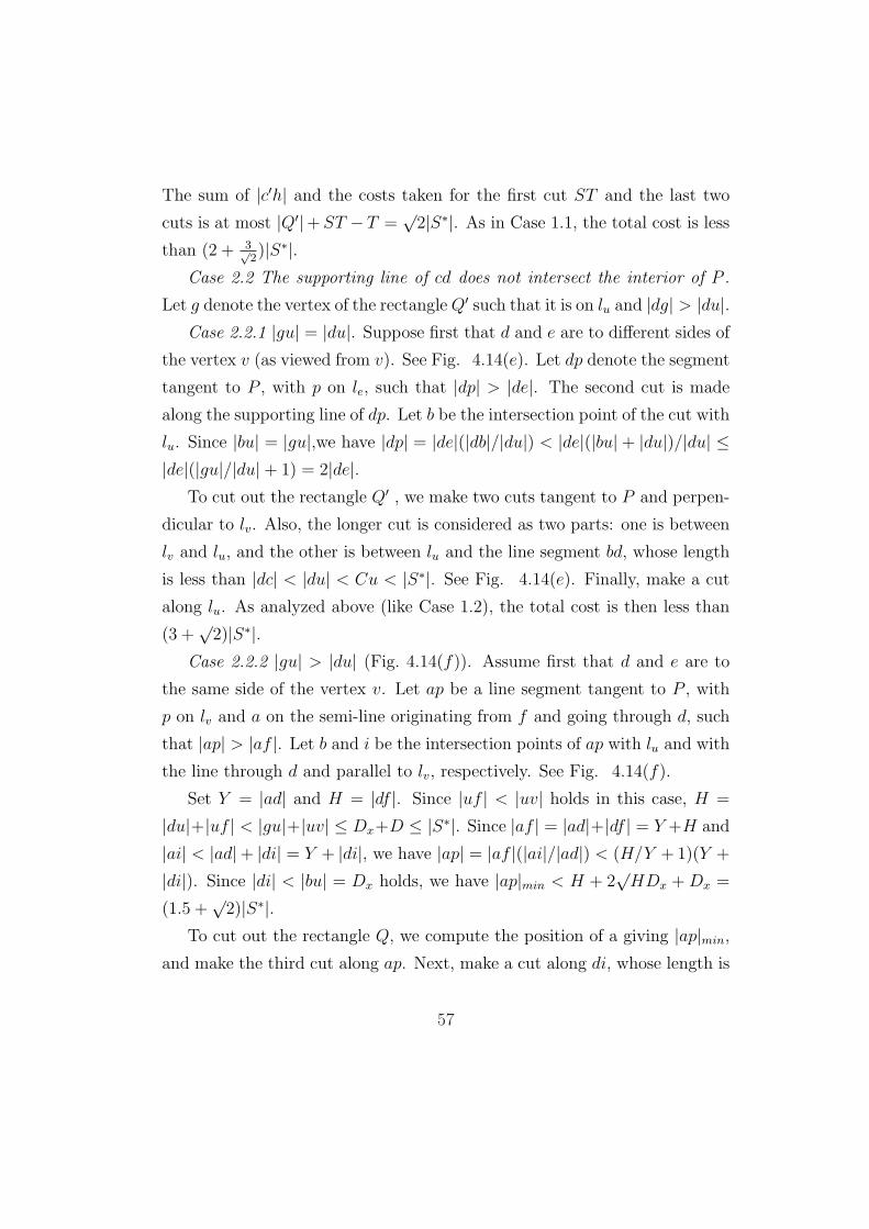
The sum of |c′h| and the costs taken for the first cut ST and the last two

cuts is at most |Q′|+ ST − T =√

2|S∗|. As in Case 1.1, the total cost is less

than (2 + 3√2)|S∗|.

Case 2.2 The supporting line of cd does not intersect the interior of P .

Let g denote the vertex of the rectangle Q′ such that it is on lu and |dg| > |du|.Case 2.2.1 |gu| = |du|. Suppose first that d and e are to different sides of

the vertex v (as viewed from v). See Fig. 4.14(e). Let dp denote the segment

tangent to P , with p on le, such that |dp| > |de|. The second cut is made

along the supporting line of dp. Let b be the intersection point of the cut with

lu. Since |bu| = |gu|,we have |dp| = |de|(|db|/|du|) < |de|(|bu|+ |du|)/|du| ≤|de|(|gu|/|du|+ 1) = 2|de|.

To cut out the rectangle Q′ , we make two cuts tangent to P and perpen-

dicular to lv. Also, the longer cut is considered as two parts: one is between

lv and lu, and the other is between lu and the line segment bd, whose length

is less than |dc| < |du| < Cu < |S∗|. See Fig. 4.14(e). Finally, make a cut

along lu. As analyzed above (like Case 1.2), the total cost is then less than

(3 +√

2)|S∗|.Case 2.2.2 |gu| > |du| (Fig. 4.14(f)). Assume first that d and e are to

the same side of the vertex v. Let ap be a line segment tangent to P , with

p on lv and a on the semi-line originating from f and going through d, such

that |ap| > |af |. Let b and i be the intersection points of ap with lu and with

the line through d and parallel to lv, respectively. See Fig. 4.14(f).

Set Y = |ad| and H = |df |. Since |uf | < |uv| holds in this case, H =

|du|+|uf | < |gu|+|uv| ≤ Dx+D ≤ |S∗|. Since |af | = |ad|+|df | = Y +H and

|ai| < |ad|+ |di| = Y + |di|, we have |ap| = |af |(|ai|/|ad|) < (H/Y + 1)(Y +

|di|). Since |di| < |bu| = Dx holds, we have |ap|min < H + 2√

HDx + Dx =

(1.5 +√

2)|S∗|.To cut out the rectangle Q, we compute the position of a giving |ap|min,

and make the third cut along ap. Next, make a cut along di, whose length is

57

less than |bu|. Two cuts, tangent to P and perpendicular to lv, are then made.

Note that the longer cut can be considered as two parts: one is between lv

and lu and the other is between lu and the supporting line of di (whose length

is less than |gu|). Finally, a cut along lu is made. The sum of |gu| and the

cost of the cut along lu is clearly less than 2Dx ≤ |S∗|. Consider now the

costs represented by |bu| and taken for the first cut along ST and two cuts

that are tangent to P and perpendicular to lv, excluding the part of the

longer cut between lu and the supporting line of di. By noticing the relation

between the segment bu and two considered vertical cuts (Fig. 4.15), we

have that the sum of these costs is less than |P |+ |ST |− |T | = |S∗|. Putting

all together, the total cost of our cutting sequence is less than (3.5+√

2)|S∗|.For the case that d and e are to different sides of v, we can also show that

the cutting cost is less than (3.5 +√

2)|S∗|. We leave the detail to readers.

It should be noted that , after finding the ST − chord in O(n) time we can

make the rest cuts in no more than O(n) time.

For cutting P out of that rectangle we follow the method used by Tan [16].

That is, we use the dynamic programming for choosing the optimal sequence

of edge cuts. In his paper Tan proved that this dynamic programming method

with all edge cuts has the maximum cutting length of (1.5 +√

2)C∗. Hence

the over all running time becomes O(n3) and the total cutting length is

less than or equal to (2√

2 + 1.5 +√

2)C∗ or 6.74 where P is centered and

(3.5 +√

2 + 1.5 +√

2)C∗ or 7.9 where P is cornered.

Hence , the following theorem holds.

Theorem 4.3.7. Algorithm2 cuts P out of Q in O(n3) time with 6.74 and

7.9 approximation ratio where P is centered and cornered respectively.

58

4.3.4 Algorithm 3

In this section we propose a polynomial time approximation scheme. We

modify the separation phase of the algorithm given by Bereg et. al [2]. They

used the separation phase same as the one Tan used. We replace it with

the separation phase of Algorithm2. Hence, we get the minimum bounding

rectangle in O(n) time with constant cut length. Next we follow the same

approach suggested by Bereg et. al which is not actually dependent on the

number of vertices of Q, hence, we can use it for our case.

Q

P

A

A′

Figure 4.15: Determining the portal points.

First of all, we determine whether P is cornered or centered in O(n)

running time. Next, we cut out a minimum area rectangle bounding P . For

this, we use the similar technique as the one we used in algorithm 4.3.3. That

is, we use the rotating calipers technique for P being centered and in P is

cornered we choose different cutting sequences in different cases as described

in 4.3.3. So, we obtain the minimum area rectangle in O(n) running time

with constant cutting cost. Hence we get an estimate EST of the cost OPT

of the optimal cutting sequence such that OPT ≤ EST ≤ cOPT , where c is

the constant approximation factor.

Next we construct a set E of candidate cuts. First put the n edge cuts

59

l2

o

q

r

p1

l1

p

Pp2

Figure 4.16: Determining the estimated cost.

into E, then, for each vertex p of P , and for each portal point v ∈ V , if the

line through both p and v specifies a valid tangent cut anchored at p (that

is, the line does not cut through P ), put the tangent cut into E. We call the

candidate cuts constructed so far the type− 1 cuts.

For every two type−1 cuts l1 and l2 intersecting at a point o and anchored

at two vertices q and r respectively (q, r,and o may coincide), we compute,

for every vertex p of P outside the triangle4oqr, all the vertex cuts anchored

at p such that the length of the cutlines segment between l1 and l2 is (locally)

minimal. We put these cuts into the candidate set E and called them the

type − 2 cuts. See Figure 4.16. The determination of a type − 2 cut can be

done in constant time [2].

Finally, in the dynamic programming step, we use dynamic program-

ming [13] to find a sequence of candidate cuts from E with the minimum

cost. This cutting sequence is our approximate solution.

We now analyze the running time of our algorithm. For the two rectangles

A and A′ ,we have |A| = O(|P |) = O(OPT )and |A′| = |A| + 8EST .Since,

EST = Θ(OPT ), we have |A′| = O(OPT ). It follows that the perimeter

60

of the polygon Q ∩ A′ is O(OPT ). The number of portal points is there-

fore O(OPT )∂EST

= O(1/∂) = O(n/ε2). The number of type − 1 cuts is O(n/ε2).

The number of type − 2 cuts is O(n2/ε4). The dynamic programming algo-

rithm [13] takes O((n2/ε4)3) = O(n6/ε12) time. Hence, We have the following

theorem

Theorem 4.3.8. Algorithm3 gives a (1 + ε) approximation scheme in poly-

nomial time.

61

Chapter 5

Searching for the Center of

Spheres and Ellipsoids

Biedl et al. [4] first posed the problem of finding the center of a circle, starting

from a point on the boundary and using a limited number of operations.

They presented an open problem for searching the center of an ellipse in

their paper. Later, Michael A. Burr [5] et al. solved that problem. But there

was still a problem in the elliptical model regarding the dead areas which

was not handled by the strategy of Michael A. Burr [5] and this problem

remained unsolved. However, in both of their works they considered the

searching space to be two dimensional. As a result their strategies do well

on a plane. But in reality the searching space is three dimensional in most

of the cases. In those cases we need an efficient strategy to find out the

center of a sphere or in some cases, the center of an ellipsoid. In this thesis

we approached the problem regarding the dead areas, proposed a model

with dead areas, suggested a way to improve the strategy regarding this and

proposed efficient strategies of searching the centers of spheres and ellipsoids

which inherently works for circle and ellipse respectively.

62

5.1 Searching the Center of Spheres

In this section we discuss about the strategy of searching the center of a

sphere efficiently.

5.1.1 Problem Description

Consider the problem of a robot searching for the center of a sphere. The

robot has only a limited number of capabilities. It can detect whether it is

inside the sphere or not, it can mark the point which it occupies, it can move

along a straight line, possibly towards a mark which it had made previously.

It can make 90 degrees and 180 degrees turns. It can detect and move to

the middle of a line segment determined by two marked end-points, if it is

on the line segment. The starting point of the robot is on the surface of the

sphere and tries to reach at the center of the sphere as quickly as possible.

Figure 5.1: Searching the center of a sphere

63

5.1.2 Mathematical Description

Let, in the Figure 5.1, S is the sphere with center located at O. The initial

position of the searching robot is at a point A on the surface of the sphere.

The target is to reach the center of the sphere as quickly as possible. The

robot has the following available operations:

1. It can detect whether it is inside the sphere or not.

2. It can mark a position.

3. It can move in a straight line, possibly toward a mark which it had

made previously.

4. It can make 90 degrees and 180 degrees turns.

5. It can move to the middle of a line segment determined by two

marked points, if it is on the line segment.

Figure 5.2: Proposed strategy.

5.1.3 Proposed Strategy

See Figure 5.2.

64

1. Leave a marker at point A.

2. Move along a straight line inside the sphere, until you reach another

surface. Let this point be B.

3. Turn 90 degrees and move along a straight line inside the sphere.

Move until you reach another surface at point C.

4. Line AB and BC are perpendicular to each other. So, A, B and

C are not co-linear [except the case where AB is the diameter of the circle

ABC , in which case B and C will be superimposed].As a result, A, B and C

lie on a single plane. Move along the perpendicular line of this plane inside

the sphere until you reach another surface at point D.

5. Mark the point D.

6. Move towards the marker of step 1, to the halfway point between two

markers

5.1.4 How to detect a direction which is inside the

sphere

Whenever the robot is told to move in a direction perpendicular to a plane

which is inside the sphere, it needs to choose between two directions. For

example, when the searching robot is at point L on the surface ABL of the

sphere and is told to move along the perpendicular direction inside the sphere

it has to choose between the direction LM and LN which are perpendicular

to the plane ABL on which the robot is standing. Now, if the object moves

along LN it will be out of the range of the transmitter, so it can understand

that the right direction should be LM . When the robot is told to move along

a perpendicular direction to a straight line when it is on the surface of the

sphere it can choose any of the direction which lies on the perpendicular plane

to that straight line as shown in Figure 5.3. The directions the robot can

choose at the point L is shown in the figure. Whether the chosen direction is

65

Figure 5.3: How to detect a direction which is inside the sphere

leading towards the inside of the sphere or not, can be decided by the above

mentioned method.

5.1.5 Correctness Proof

Now we prove that the strategy leads a robot starting from the surface of a

sphere to the center of that sphere.

Lemma 5.1.1. Every cross section of a sphere produces a circular plane.

Proof. We can easily prove this by solving the equations of a sphere and a

plane. In Figure 5.4, we show how a plane cuts a sphere without the loss

of generality. In the same figure, we can see the resultant circular surface

yielded by that cut. Finally in Figure 5.4, we get a top view of that circular

plane.

Lemma 5.1.2. The straight line joining the center of the sphere and the

66

Figure 5.4: Cross section of a sphere

center of the circular plane produced by a cross-section of that sphere is per-

pendicular to that plane.

Figure 5.5: The straight line joining the center of the sphere and the center of

the circular plane produced by a cross-section of that sphere is perpendicular

to that plane.

Proof. Let, S be a sphere with center at T . ABC is a circular plane produced

by a cross-section of the sphere. P is the center of the circular plane, ABC.

We join T ,P . According to this lemma TP is perpendicular to the plane

67

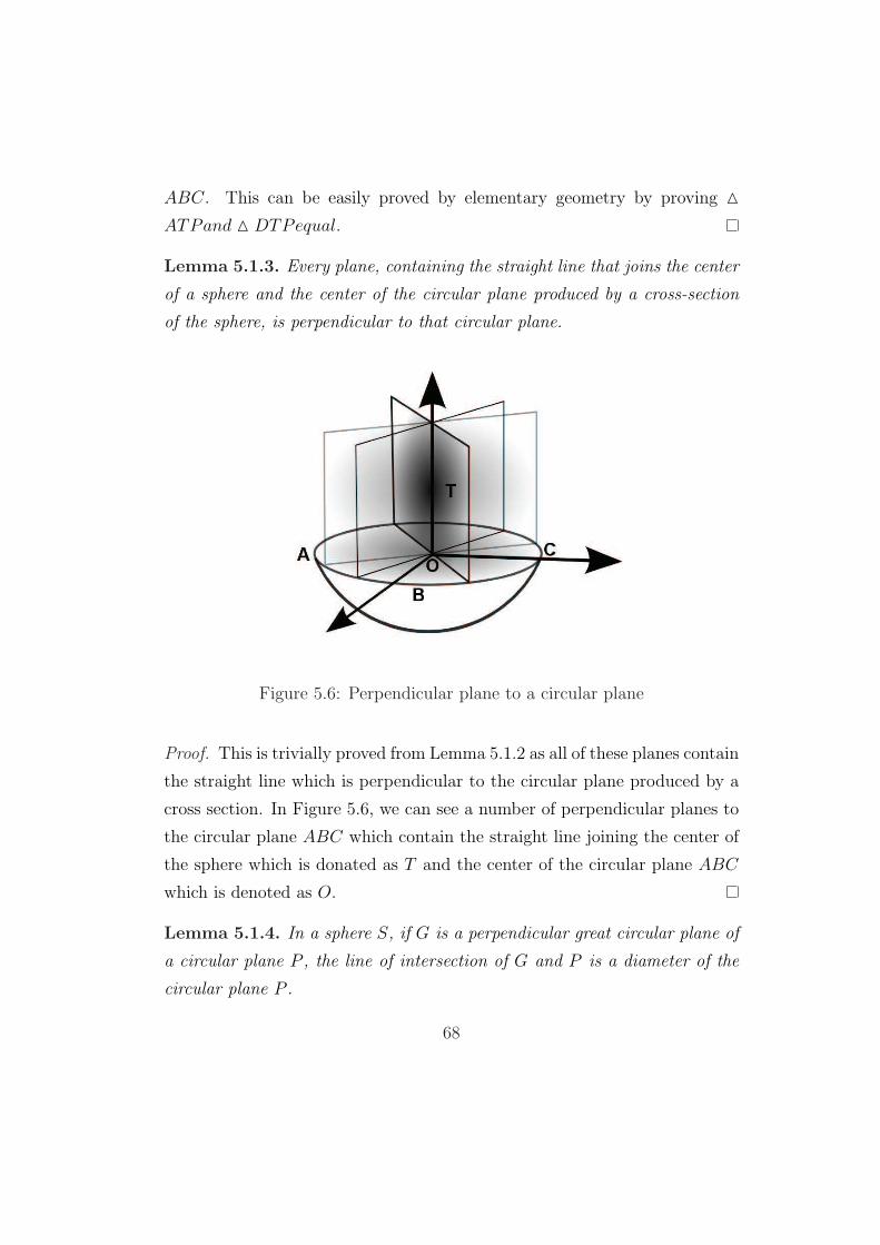
ABC. This can be easily proved by elementary geometry by proving MATPand M DTPequal.

Lemma 5.1.3. Every plane, containing the straight line that joins the center

of a sphere and the center of the circular plane produced by a cross-section

of the sphere, is perpendicular to that circular plane.

Figure 5.6: Perpendicular plane to a circular plane

Proof. This is trivially proved from Lemma 5.1.2 as all of these planes contain

the straight line which is perpendicular to the circular plane produced by a

cross section. In Figure 5.6, we can see a number of perpendicular planes to

the circular plane ABC which contain the straight line joining the center of

the sphere which is donated as T and the center of the circular plane ABC

which is denoted as O.

Lemma 5.1.4. In a sphere S, if G is a perpendicular great circular plane of

a circular plane P , the line of intersection of G and P is a diameter of the

circular plane P .

68

Figure 5.7: Figure for Lemma 5.1.4.

Proof. By the definition of the perpendicular great circular plane G will

contain the axis diameter of the circular plane, P . The axis diameter is

perpendicular to the circular plane, P . Moreover, the center of the sphere

lies on the axis-diameter. Now, from lemma 5.1.1 we know that the straight

line, L (line TC in the Figure 5.7) joining the centers of the sphere and center

of P is perpendicular to P . So, L must be a part of the axis- diameter of P .

Hence the center of P must lie on G. More preciously it will lie on the line of

intersection of the planes P and G, namely AB. Now,∠ACT = ∠BCT = 90

degrees and A, C and B lie on the plane G. so,∠ACT + ∠BCT = 180

degrees. Hence A,C and B are co- linear. Moreover the line segment AB

passes through the center of the circular plane P . So, AB is the diameter of

the circular plane P . Hence, proved.

69

Correctness of the Strategy

According to the right angle strategy described by T. Beidl et al. [4], the

robot can reach from one end to the other end of a diameter of a circle

with two mutually perpendicular moves as shown in the Figure 5.8.Hence, if

we apply this strategy on a circular plane produced by a cross-section of a

given sphere, it would lead us from one end point to another end point of a

diameter of that circular plane. Now we consider the great circular plane G

described by the great circle ACE. G is perpendicular great circular plane

for the circular plane P , described by ABC and produced by a cross section

of the sphere. If the robot moves with right angle strategy on the plane P

Figure 5.8: Correctness of the strategy

starting from the point A, it would lead the robot to C which is the opposite

end point of the diameter AC. Without the loss of generality we assume that

G intersects P along the line AC and it is always true that G will intersect

P with a straight line which is a diameter of P by Lemma 5.1.5. Now, we

consider the circle ACE. To reach the center of the sphere, the robot needs

to reach the center of this great circle. If we think about applying the right

angle strategy on the circle ACE , we find that the robot has just completed

one of first two perpendicular moves which leads the robot from one endpoint

to the another endpoint of a diameter of the circle ACE by moving from A

70

to C. So, now it needs to move along a line perpendicular to AC and our

strategy suggests the same by telling it to move along the straight line which

is perpendicular to the plane, P .

Figure 5.9: Correctness proof

Moving along that direction the robot reaches at E on the surface. Now,

according to the right angle strategy, the robot has to move toward the point,

A. and on the half way it will reach the center of the circle, ACE. And as,

ACE is a great circle for the sphere S, it will eventually reach the center

of the sphere. So, the strategy correctly leads the robot to the center of a

sphere.

5.2 Competitive Ratio

The total length of traversal is [2R sin x(sin y + cos y) + 2R cos x + R] which

gives the competitive ration of at most 3.82. This strategy needs only 4

moves and 2 markers for a single searcher to reach the center.

71

Figure 5.10: Competitive ratio calculation

5.3 Detection Stage of Searching the Center

of an Ellipsoid

5.3.1 Problem Description

This problem is almost similar to the problem of searching the center of a

sphere. The only difference is that we are considering here the searching

space as an ellipsoid. In their paper T. Beidl et al. [4] claimed that the

searching area is not bounded by a circle in reality. It is actually elliptical.

So, strategy for finding out the center of an ellipse was necessary which was

later done by Michael A. Burr [5]. In three dimensional spaces we can think

this model as an ellipsoidal. So, now the mission is to find out the center

of that ellipsoid for that same robot which has the capabilities mentioned

earlier in this thesis.

5.3.2 Our Work

The strategy of Michael A. Burr [5] works well for an ellipse on a plane but it

is not suitable for three dimensional cases, where the searching space should

72

be modelled as an ellipsoid. We have proposed here an efficient strategy for

searching the center of an ellipsoid. Before we propose our strategy, we would

like to discuss some properties of an ellipsoid. These properties along with

the strategy of Michael A. Burr [5] will lead us to the proposed strategy.

Lemma 5.3.1. A plane cuts an ellipse to an ellipsoid.

Figure 5.11: Figure for Lemma 5.3.2

This property can easily be proved by solving the equations of an ellipsoid

and a plane.

Lemma 5.3.2. We can always have a projection of an ellipsoid with two

parallel elliptical planes inside it which are the planes of intersection of the

ellipsoid with two parallel planes, where the ellipsoid is an ellipse and those

parallel planes are two parallel chords of it.

From the physical property of ellipsoid, we know that any projection of

an ellipsoid is an ellipse. So, if we chose to project the ellipsoid in a way that

the parallel planes will be projected as parallel lines, we are done.

Lemma 5.3.3. Two parallel elliptical planes produced by the intersection of

an ellipsoid with two parallel planes have their centers on a diameter of the

ellipsoid.

73

Figure 5.12: Figure for Lemma 5.3.3

Let us consider the Figure 5.13. Here the ellipsoid E is intersected by

two parallel planes resulting two parallel elliptical-shaped planes inside it.

We name them A and B. If we join the centers of the elliptical planes A

and B and extend the line we shall get a chord which is claimed to be a

diameter by this lemma. Hence the midpoint of this chord will be the center

of the ellipsoid. This can be easily proved by using the lemma 5.1.7. On the

projection of the ellipsoid, we get an ellipse with two parallel chords. The

line joining the midpoints of those parallel chords will produce a diameter

of that ellipse. That diameter of the ellipse is actually the projection of a

diameter of the ellipsoid. Hence, we are done.

5.3.3 Proposed Strategy

1.Find the center of the ellipse as told in the thesis of Michael A.

Burr [5] and mark the center.

74

Figure 5.13: Proposed strategy

2.Go to any of the two antipodal points of the last diameter used in

that searching inside that ellipse.

3.Go along the perpendicular line of that plane until the signal fades.

4. Now, re-execute that strategy of Michael A. Burr [5] and find out

the center of that ellipse and mark it.

5.Go toward the previously marked center and keep going until the

signal fades and mark this point.

6.Turn 180 degrees and keep going until the signal fades and mark

that point.

7.Go to the midpoint of the last two marked points.

5.3.4 Correctness

This strategy is the direct consequence of the strategy used for searching the

center of an ellipse. We apply the strategy using the Lemma 5.1.8 we can

prove it instantly. So, this strategy will certainly lead the robot toward the

center of an ellipsoid.

75

5.4 Correction Stage

In the correction stage we handle the problem with dead areas for an ellipse.

We describe the correction stage for both ellipse and ellipsoid. First of all

we concentrate to the case of an ellipse and its dead areas. Then we advance

to the case of an ellipsoid. The concept of elliptical model comes from the

idea that the shape of the electromagnetic field of the transceiver is similar

to that of a magnetic field of a magnet. Michael A. Burr [5] showed a model

in his paper which is shown bellow.

Figure 5.14: Electromagnetic field

But this model is not realistic according to our point of view because the

dead regions are not so narrow near the transceiver in reality. So, we propose

here a hypothetical model assuming the transceiver as a bar magnet. A bar

magnet has two poles, the North Pole and the South Pole. The magnetic

force lines are assumed to be emitted from the North Pole and enters into the

South Pole as showed in the Figure 5.14. So the electromagnetic field takes

the shape of Figure 5.15 which is composed of two elliptical lobes. The center

of the magnet is at C which we have to find out. The two ellipses are assumed

to be symmetric with respect to the axis of the magnet for our purpose. Now,

the boundary of the electromagnetic field looks like Figure 5.16. We assume

76

Figure 5.15: Magnetic Field

that this field is bounded by a larger ellipse such a way that the center of the

ellipse is the center of the magnet, C. It is obvious that the signal cannot

reach to every point inside that ellipse. Figure 5.17 explains the idea. In

this figure, E is the large ellipse surrounding the electromagnetic field and C

is the center of the magnet as well as the center of the large ellipse. D1 and

D2 are the dead regions where no signal reaches. The searching agent starts

searching from any point on the dotted lines and the mission is to reach at

C.

Due to these dead regions the parallel chord strategy of Michael A.

Burr [5] may fail to reach at C. Figure 5.18 describes such a case where the

strategy fails to guide the searcher to the center. The strategy ends at point

F where the original center of the ellipse is located at point C.

We use here a hypothetical assumption on this model. We assume that,

if we take two mutually perpendicular chords of the larger ellipse which

have the same midpoint, not both of them will go through the dead regions.

Using this assumption along with this model, we propose here a strategy

77

Figure 5.16: Revised elliptical model

Figure 5.17: Assumed model

which will improve the searching accuracy. In the worst case, this scheme

will result the same point resulted by the detection stage. So, it has no side-

effect. Moreover, this strategy can detect the worst case quickly and ends

up immediately. Even if, our hypothetical model is not the one really exists,

still this strategy returns the same point we got in the detection stage and

ends up sharply.

78

Figure 5.18: Dead regions

Figure 5.19: Wrong result by proposed strategy

5.4.1 Proposed Correction Strategy

1.Apply the parallel chord strategy reach the point of 1st assumption.

Remember the last diameter used to get the center. Name that diameter

D(k). Mark the center , name it C(k).

2. Turn 90 degrees and get another Diameter D(k+1) and its midpoint

C(k + 1).

3. Compute the distance between C(k) and C(k + 1). If its less than

a predefined fixed value p then C(k + 1) is the refined result. break and end

the process. If the distance is greater than p then let D(k) = D(k + 1) and

C(k) = C(k + 1). Go to step 2.

79

5.4.2 Convergence of the strategy

This strategy will certainly converge to a certain point because of the central

tendency of the ellipse. In each step the midpoints will lead the searcher

closer to the center of the ellipse if the diameter is not affected by the dead

regions. No two consecutive diameters will be affected by the dead region by

the hypothesis. So, this strategy will converge to the center of the ellipse.

For example we can apply this strategy for the case stated in Figure 5.18

where the parallel chord method failed to reach the center. In Figure 5.19,

we show how our strategy refines the solution and reaches the center.

Figure 5.20: Correction strategy

5.4.3 Performance Analysis

If our hypothesis matches the case, the center of the ellipse will be reached

very soon. The actual length of the traversed path in correction stage is a

function of the point returned by the detection stage and the last diameter

used in that stage and the predetermined fixed value p. So, there exists a

function F (D,C, p) describing the length of the traversal. The growth of this

function is expected to be reduced at a rate which is a logarithmic function

of A and B , where A and B are the length of the two axes of the large

ellipse and C is the center returned by the detection stage and D is the last

80

diameter used in that stage. The upper bound of this function is roughly

estimated as O([A ∗ log(B) + B ∗ log(A)]).

5.4.4 Worst Case Analysis

In the worst case the model with the hypothesis may fail and both of the

first two consecutive chords of correction stage will be affected by the dead

regions. In that case both of the chords are in fact the chords of one of the

smaller elliptical lobes. As a result, first two midpoints will be close enough

to end the strategy. In other words , the strategy will end up with the same

result of the detection stage and it will take only the cost of travelling one

chord and determining its midpoint , more preciously O((3/2) ∗ (A + B)).

5.4.5 For Ellipsoids

For the correction steps in ellipsoids , we do the almost same thing with three

consecutive chords. After reaching the point returned by the detection steps

, we shift the point to the midpoint of the perpendicular chord drawn at that

point. Then we take another chord perpendicular to that plane and shift

the assumed center to the midpoint of that chord. In this way, we gradually

approach the center of the ellipsoids.

5.5 Use of Volume Knobs

If we use the volume knobs of the transceiver, sometimes the searching can

be even easier. The volume button can be used at the detection stage. We

used the strategies of finding the center of circles and spheres to determine

the center of spheres and ellipsoids. So, the technique of using volume in

searching the center of circles or ellipses can be used in those steps.

81

Chapter 6

Conclusion and Future Works

In this thesis we have studied the minimization of the length for the cutting

a convex polygon out of a circle and the efficient strategy to search the center

of a sphere or an ellipsoid. In particular we studied four types of problems:

(i) cutting a cornered convex polygon out of a circle, (ii) cutting a centered

polygon out of a circle, (iii) searching for the center of a sphere and (iv)

searching for the center of an ellipsoid. Below we discuss the summary of

our results, their applications and some possible future works associated with

those.

6.1 Cutting a cornered polygon out of a circle

We have studied the problem of cutting a cornered convex polygon out of a

circle using line cuts. We have given an algorithm with runs in linear time

and has an approximation ratio of O(n). We have also given a 6.74 constant

factor approximation algorithm with runs in O(n3) time. Before our works

there were no works done to cut a polygon out of a circle. We are the first

to work on this to our knowledge. And comparing to the algorithms so far

given by the researchers for cutting a polygon out of another, our algorithm is

82

parallel in running time and approximation ratio. Moreover, we are hopeful

to extend our algorithm to device another useful way to cut out a polygon

out of another in similar fashion which will oversmart the currently used

algorithms.

6.2 Cutting a centered polygon out of a circle

We have studied the problem of cutting a centered polygon out of a circle. We

have given an algorithm which runs in linear time and has an approximation

ration of O(logn). We have also given an constant factor of 7.9 algorithm

which runs in O(n3) time.

We have merger the algorithms for cornered and centered convex polygon

to get the general solution of cutting a convex polygon out of a circle. For

determining whether a convex polygon is cornered of centered we have also

given a linear time algorithm.

Finally, we have given a polynomial time approximation scheme(PTAS)

for this problem.

Minimizing the cutting length of a geometric shape out of another one

is particularly important in metal cutting industries. It is also important in

diamond cutting industries. In computer graphics it can be helpful in render-

ing different geometric shapes to different frames. In some very recent works

we see that robot-surgeons are used to execute critical operations. Cutting

certain portions of human body by a robot can be aided by minimizing the

necessary cutting length. So, this algorithms are of enormous use both in

the theoretical fields and application of industry and medical science.

We have worked only on line cuts. The similar problems on ray cuts

are still to be approached. The approximation ratio can be improved. The

running time of the constant factor algorithm may get improved by using

rotating calipers algorithms. The PTAS may get improved by using better

83

heuristics.

6.3 Searching for the center of a sphere

We have studied the problem of searching the center of a sphere. The strat-

egy for searching for the center of a circle was previously given by various

researchers. But no algorithm was given for the three dimensional cases.

The two dimensional searching strategy is not applicable for three dimen-

sional searching spaces. So, we have given an efficient strategy find out the

center of a sphere under certain limitations. We have also shown that our

strategy is correct and efficient. We have also suggested the solutions when

multiple signal level detection nobs are present.

6.4 Searching for the center of an ellipsoid

We have studied the problem when we have to search the center of an ellipsoid

under definite constraints. For a robot with minimum signal detection power

our given algorithm can search the center of an ellipsoid.

The algorithm of searching the center of an ellipse suffers from the prob-

lem of dead regions, so does the algorithm for searching the center of an

ellipsoid. In this thesis we have given a strategy which can be helpful in

avoiding the dead region problem. This strategy can be improved by using

different geometric property of ellipsoids.

The application of and efficient searching strategy of the center of an

sphere or an ellipsoid can be helpful in searching lost objects in binary detec-

tion sensor networks. It can also be used in monitoring traffic in busy roads

and the detection of lost starts in space. If we can extend the algorithm in

may be useful in determining the shape of black holes, too.

84

Index

Approximation algorithm, 26

Approximation ratio, 27

Axis Diameter, 24

Centered Convex Polygon, 21

computational geometry

definition, 1

dynamic problems, 4

geometric problem, 3

main branches, 2

research areas, 2

static problem, 2

computational geometry’s application,

6

concave polygon, 21

Constant factor approximation algo-

rithm, 27

convex polygon, 20

cornered convex polygon, 21

curving phase, 43

cut and uncut edges, 23

cutting sequence, 22

D-separation, 36

Edge Cut, 21

Great Circle, 24

line cut, 22

NP-Complete problem, 25

NP-Hard problem, 26

obtuse phase, 41

optimal solution, 26

optimization problem, 26

Perpendicular Great Circular Plane,

24

Polynomial time approximation scheme,

27

ray cut, 23

triangle separation, 39

Vertex Cut, 21

Visible edges, 23

85

Bibliography

[1] Syed Ishtiaque Ahmed, Md. Ariful Islam and Masud Hasan, “Cutting

a cornered convex polygon out of a circle,” International Conference

on Computer and Information Technology (ICCIT), 2008.

[2] Sergey Bereg , Ovidiu Daescu, and Minghui Jiang, “A PTAS for Cut-

ting Out Polygons with Lines,” COCOON 2006, LNCS 4112, pp. 176-

185, 2006.

[3] J. Bhadury and R. Chandrasekaran, “Stock cutting to minimize cutting

length,” European Journal of Operations Research, 88:69-87, 1996.

[4] T. Biedl, M. Hasan, J. D. Horton, A. Lopez- Ortiz, and T. Vinar.

Searching for the center of a circle. Proceedings of the 14th Cana-

dian Conference on Computational Geometry (CCCG02), pages137141,

2002.

[5] Michael Burr, Alexandra Lauric, and Katelyn Mann, Searching for the

center of an ellipse. Proceedings of the 14th Canadian Conference on

Computational Geometry (CCCG05), pages 260-263, 2005.

[6] D. A. Brannan, M. F. Esplen, and J. J. Gray. Geometry. Cambridge

University Press, 1(1):1999.

[7] Ramaswamy Chandrasekaran, Ovidiu Daescu, and Jun Luo, “Cutting

86

Out Polygons,” In Preecidings of the 17th Canadian Conference on

Computational Geometry, pages 183-186, 2005.

[8] Ovidiu Daescu and Jun Luo, “Cutting out polygons with lines and

rays,” Computational Geometry: International Journal of Computa-

tional Geometry and Applications, 16(2-3):227-248, 2006. (Preliminary

version in Proceedings of the 15th Annual International Symposium on

Algorithms and Computation (ISAAC’04), LNCS 3341, pages 669-680,

2004.)

[9] Erik D. Demaine, Martin L. Demaine, and Craig S. Kaplan, “Polygons

cuttable by a circular saw,” Computational Geometry: Theory and

Applications, 20:69-84, 2001.

[10] Adrian Dumitrescu, “An approximation algorithm for cutting out con-

vex polygons,” Computational Geometry: Theory and Applications,

29:223-231, 2004. (Preliminary version in Proceedings of the 14th

Annual ACM-SIAM Symposium on Discrete Algorithms (SODA’03),

pages 823-827, 2003.)

[11] Adrian Dumitrescu, “The cost of cutting out convex n-gons,” Discrete

Applied Mathematics,143(1-3):353-358, 2004.

[12] K. Mehlhorn, T. C. Shermer, and C. K. Yap. A complete roundness

classification procedure. In SCG 97: Proceedings of the thirteenth

annual symposium on Computational geometry, pages 129138. ACM

Press, 1997.

[13] Mark H. Overmars and Emo Welzl, “The complexity of cutting paper,”

Proceedings of the 1st Annual ACM Symposium on Computational Ge-

ometry (SoCG’85), pages 316-321, 1985.

87

[14] R. I. Perla and M. M. Jr. Avalanche Handbook. US Department of

Agriculture, July 1976.

[15] M. G. Smith. A complete roundness classification procedure.

Avalanche transceiver recovery skills: Tips and traps, GearWorld

www.gearworld.com, 1998.

[16] Xuehou Tan, “Approximation algorithms for cutting out polygons with

lines and rays,” Proceedings of the 11th International Computing and

Combinatorics Conference (COCOON’05), LNCS 3595, pages 534-543,

2005.

[17] Godfried Toussaint, “Solving geometric problems with the rotating

calipers,” Procs. MELECON, Athens, Greece, 1983.).

88

algorithms in computational geometry - sbumdaislam/thesis.pdf · b.sc. engg. thesis algorithms in...

Documents