algorithms for regression and classification

Algorithms for Regression and ClassificationRobust Regression and Genetic Association Studies

Dissertation

zur Erlangung des Grades eines

Doktors der Naturwissenschaften

der Technischen Universität Dortmund

an der Fakultät für Informatik

von

Robin Nunkesser

Dortmund

2009

Tag der mündlichen Prüfung: 24.02.2009

Dekan: Professor Dr. Peter Buchholz

Gutachter: Juniorprofessor Dr. Thomas JansenProfessor Dr. Roland Fried

iii

Abstract

Regression and classification are statistical techniques that may be used to extractrules and patterns out of data sets. Analyzing the involved algorithms comprises in-terdisciplinary research that offers interesting problems for statisticians and computerscientists alike. The focus of this thesis is on robust regression and classification ingenetic association studies.

In the context of robust regression, new exact algorithms and results for robustonline scale estimation with the estimators Qn and Sn and for robust linear regressionin the plane with the estimator least quartile difference (LQD) are presented. Addi-tionally, an evolutionary computation algorithm for robust regression with differentestimators in higher dimensions is devised. These estimators include the widely usedleast median of squares (LMS) and least trimmed squares (LTS).

For classification in genetic association studies, this thesis describes a Genetic Pro-gramming algorithm that outpeforms the standard approaches on the considered datasets. It is able to identify interesting genetic factors not found before in a data set onsporadic breast cancer and to handle larger data sets than the compared methods. Inaddition, it is extendible to further application fields.

v

Acknowledgments

First and foremost, I would like to thank my former advisor Ingo Wegener (4 December1950 – 26 November 2008) for providing the topic of this dissertation, giving valuableadvice and supporting and encouraging me. I am grateful that I had the fortune towork with him.

I would also like to thank my colleagues at the chair of Efficient Algorithms andComplexity Theory at the Faculty of Computer Science of the TU Dortmund Univer-sity and my colleagues in the SFB 475 Reduction of complexity in multivariate datastructures. Especially I would like to thank my advisors Thomas Jansen and RolandFried and my not yet mentioned co-authors Thorsten Bernholt, Ursula Gather, KatjaIckstadt, Joachim Kunert, Oliver Morell, Karen Schettlinger, and Holger Schwender.

Many proofreaders gave valuable advise that improved this thesis. I also thankevery proofreader and reviewer that was not mentioned here by name.

I gratefully acknowledge the financial support of the Deutsche Forschungsgemein-schaft (SFB 475, Reduction of complexity in multivariate data structures).

Molecular graphics images were produced using the UCSF Chimera package fromthe Resource for Biocomputing, Visualization, and Informatics at the University ofCalifornia, San Francisco (supported by NIH P41 RR-01081).

Finally, I thank my family and friends for all the things in life besides computerscience.

Contents

I Introductory Part 1

1 Introduction 3

2 Overview of Publications 7

II Robust Statistics 9

3 Preliminaries 113.1 Robust Linear Regression . . . . . . . . . . . . . . . . . . . . . . . . . 133.2 Robust Scale Estimation . . . . . . . . . . . . . . . . . . . . . . . . . . 16

4 Online Computation of Two Estimators of Scale 194.1 Motivation . . . . . . . . . . . . . . . . . . . . . . . . . . . . . . . . . . 204.2 Online Computation with Moving Windows . . . . . . . . . . . . . . . 214.3 Computation of Qn . . . . . . . . . . . . . . . . . . . . . . . . . . . . . 224.4 Computation of Sn . . . . . . . . . . . . . . . . . . . . . . . . . . . . . 33

5 Computing the Least Quartile Difference Estimator in the Plane 395.1 The Concept of Geometric Duality . . . . . . . . . . . . . . . . . . . . 405.2 Computing the LQD Geometrically . . . . . . . . . . . . . . . . . . . . 425.3 Solving the Underlying Decision Problem . . . . . . . . . . . . . . . . . 455.4 Searching for the Optimal Point . . . . . . . . . . . . . . . . . . . . . . 465.5 Running Time Simulations . . . . . . . . . . . . . . . . . . . . . . . . . 51

6 An Evolutionary Algorithm for Robust Linear Regression 536.1 Evolutionary Computation . . . . . . . . . . . . . . . . . . . . . . . . . 546.2 Outline of the Algorithm . . . . . . . . . . . . . . . . . . . . . . . . . . 556.3 Comparison . . . . . . . . . . . . . . . . . . . . . . . . . . . . . . . . . 58

III Genetic Association Studies 61

vii

viii

7 Preliminaries 637.1 Single Nucleotide Polymorphisms . . . . . . . . . . . . . . . . . . . . . 637.2 Genetic Programming . . . . . . . . . . . . . . . . . . . . . . . . . . . 647.3 Hypothesis Testing . . . . . . . . . . . . . . . . . . . . . . . . . . . . . 65

8 Genetic Programming for Association Studies 698.1 Boolean Concept Learning . . . . . . . . . . . . . . . . . . . . . . . . . 698.2 Genetic Programming Algorithm . . . . . . . . . . . . . . . . . . . . . 718.3 Automated Rules to Select the Best Individual . . . . . . . . . . . . . 778.4 Results on Real and Simulated Data . . . . . . . . . . . . . . . . . . . 798.5 Logic Minimization . . . . . . . . . . . . . . . . . . . . . . . . . . . . . 86

IV Concluding Part 91

9 Conclusions 93

10 Classifying with Decision Diagrams 9510.1 Ordered Decision Diagrams . . . . . . . . . . . . . . . . . . . . . . . . 9710.2 Ideas for Adaptions . . . . . . . . . . . . . . . . . . . . . . . . . . . . 98

Bibliography 99

List of Algorithms 111

List of Figures 113

List of Tables 115

Index 117

Part I

Introductory Part

1

1 Introduction

In an early article dealing with the interface of computer science and statistics Shamos(1976) wrote:

From the viewpoint of applied computational complexity, statistics is a goldmine, for it provides a rich and extensive source of unanalyzed algorithmsand computational procedures.

Based on this “gold rush” of the late 1960s and early 1970s a two-way feedback betweencomputer science and statistics has since been established (see e. g. Gentle et al.,2004 for more historic background). In 1967, the first joint conference Symposiumon the Interface of Computer Science and Statistics was held. The attendance atthe Interface Symposia grew rapidly in the 1970s. Besides these Interface Symposia,the 1970s also saw the formation of further collaborative conferences and societies.In the 1980s, when rapidly growing computing capabilities and computer availabilitychanged many sciences, the importance of interdisciplinary research grew even more.In statistics, the advances in computer technology enabled statistical methods, thatwere not practicable before. However, statistical methods with high computationalcomplexity may probably never be computed exactly in a reasonable amount of time.The high computational complexity of many statistical methods is only one of manyreasons why statistics still offers many interesting problems for computer scientists.In fact, the rich and extensive source of unanalyzed algorithms and computationalprocedures will not run dry for a long time to come.

This thesis deals with two topics at the interface of computer science and statisticsfrom a computer scientist’s perspective. One topic is computational biology, whichemerged very recently as a multidisciplinary field involving both sciences. The othertopic is robust statistics, in particular robust regression.

Regression analysis is a technique to model the relationship between a responsevariable and one or more explanatory variables. In linear regression, the mean or themedian of the response variable is modeled as a linear combination of the explanatoryvariables. The best known linear regression method is least squares, which dates backto Gauss and Legendre (for historical discussions of least squares see Plackett, 1972;Stigler, 1981). One of the advantages of least squares is that it is has a closed formsolution. A disadvantage is that a single outlying value can have arbitrarily largeeffects on the estimation. The aim of robust regression is to bound unduly effects ofinfluence factors like outlying values. One of the earliest linear regression methodsto be more robust than least squares is least absolute deviations, which is attributed

3

4 1 Introduction

to Laplace (for a brief history and comparison with least squares see Portnoy andKoenker, 1997). Although published earlier it is not as popular as least squares,which is mostly due to its computational complexity. In fact, Bernholt (2005) provesthat many robust regression methods are NP-hard, which underlines the need for goodheuristics and for algorithms for manageable cases like low dimensional data. Afterthe introductory Part I of this thesis, we consider new algorithms for some robustmethods in Part II. Apart from the regression methods, we also consider two otherestimators that are helpful in the context of regression. When conducting regressionanalyses, one frequently needs an auxiliary estimation of the variability of a variableor a probability distribution. For this purpose, estimators of scale like the standarddeviation are used. The standard deviation is a non-robust estimator and algorithmsfor robust alternatives are of high interest. Thus, we provide new algorithms for tworobust estimators of scale in Part II in addition to the algorithms for robust regressionmethods.

Part III deals with genetic association studies which is a topic from computationalbiology. The aim of these studies is to identify genetic factors that may contribute to amedical condition, for example, a specific type of cancer. Among the most importantgenetic factors considered are single nucleotide polymorphisms, i. e. genetic variationsthat occur when different base alternatives exist at a single base pair position of theDNA. In this thesis, we mainly cover the classification problem of identifying geneticfactors that distinguish between having the medical condition under consideration andnot having it. To this end, we consider a genetic programming (Koza, 1992) algorithmfor finding prediction models based on single nucleotide polymorphism data.

In detail, following this introduction, Chapter 2 gives an overview of the publica-tions underlying this thesis and the contribution of the author. The part of the thesisconcerned with robust regression starts with Chapter 3, which introduces the neededfundamentals of robust statistics. The first new results are presented in Chapter 4,which contains new online algorithms for the robust scale estimators Qn and Sn out-performing existing algorithms. In Chapter 5, we consider an estimator called leastquartile difference (LQD) which is based on the scale estimator Qn. We show thatcomputation of the LQD in the plane is possible in time O(n2 log2 n) or expected timeO(n2 log n) and state known algorithms achieving this bounds. The bounds are farlower than the hitherto known time bound of O(n4). Additionally, we present two newalgorithms that almost perform within the theoretically possible runtime. Both algo-rithms are advantageous in terms of applicability and simplicity of implementation.

In Chapter 6 we use evolutionary computation for NP-hard robust regression meth-ods in higher dimensions. The provided algorithm enables us to compute good solu-tions for least median of squares, least quantile of squares, least quartile difference,least trimmed squares, least trimmed sum of absolute values, and similar estimators.We also compare this new heuristic to existing ones and show its advantages.

Part III starts with Chapter 7 giving an introduction to genetic association studies.After these preliminaries, Chapter 8 introduces a new genetic programming algorithm

5

for genetic association studies called GPAS. The comparison of GPAS with state-of-the-art algorithms indicates a superior performance in the investigated situations. Inaddition, the algorithm is not restricted to the intended application field, but may alsobe applied to other tasks, for example, logic minimization.

In the final part, Chapter 9 provides some conclusions and research outlooks. Theconcluding Chapter 10 gives a detailed outlook on a genetic programming algorithmfor another classification problem in genetic association studies, namely classificationwith more than two classes.

6 1 Introduction

2 Overview of Publications

Some of the material covered in this thesis has previously been published in journals,conference proceedings, or as technical reports. Table 2.1 gives an overview of thesepublications, the contribution of the author to the respective publications, and thepart of this thesis each publication contributes to. The first of the listed publicationsis also the basis for a section in the Ph.D. thesis of Bernholt (2006).

Publication Contributionof the author

Correspondingchapter

Bernholt, Nunkesser, and Schettlinger (2007) 45% Chapter 5Nunkesser, Bernholt, Schwender, Ickstadt, andWegener (2007)

45% Chapter 8

Nunkesser, Schettlinger, and Fried (2008) 40% Chapter 4Nunkesser (2008) 100% Chapter 8Morell, Bernholt, Fried, Kunert, and Nunkesser(2008)

25% Chapter 6

Nunkesser and Morell (2008) 90% Chapter 6Nunkesser, Fried, Schettlinger, and Gather (2009) 40% Chapter 4

Table 2.1: Overview of underlying publications and the contribution of the author

List of Publications

1. Bernholt, T., Nunkesser, R., and Schettlinger, K. (2007). Computing the leastquartile difference estimator in the plane. Computational Statistics & DataAnalysis , 52(2), 763–772. http://dx.doi.org/10.1016/j.csda.2006.12.039

2. Nunkesser, R., Bernholt, T., Schwender, H., Ickstadt, K., and Wegener, I. (2007).Detecting high-order interactions of single nucleotide polymorphisms using ge-netic programming. Bioinformatics , 23(24), 3280–3288. http://dx.doi.org/10.1093/bioinformatics/btm522

3. Nunkesser, R., Schettlinger, K., and Fried, R. (2008). Applying the Qn estimatoronline. In C. Preisach, H. Burkhardt, L. Schmidt-Thieme, and R. Decker, edi-tors, Data Analysis, Machine Learning and Applications , Studies in Classifica-

7

http://dx.doi.org/10.1016/j.csda.2006.12.039

http://dx.doi.org/10.1093/bioinformatics/btm522

http://dx.doi.org/10.1093/bioinformatics/btm522

8 2 Overview of Publications

tion, Data Analysis, and Knowledge Organization, pages 277–284, Berlin, Heidel-berg. Springer-Verlag. http://dx.doi.org/10.1007/978-3-540-78246-9_33

4. Nunkesser, R. (2008). Analysis of a genetic programming algorithm for asso-ciation studies. In GECCO ’08: Proceedings of the 10th Annual Conferenceon Genetic and Evolutionary Computation, pages 1259–1266, New York. ACM.http://doi.acm.org/10.1145/1389095.1389339

5. Morell, O., Bernholt, T., Fried, R., Kunert, J., and Nunkesser, R. (2008). Anevolutionary algorithm for lts-regression: A comparative study. In P. Brito,editor, COMPSTAT 2008: Proceedings in Computational Statistics , volume II(Contributed Papers), pages 585–593, Heidelberg. Physica-Verlag.

6. Nunkesser, R. and Morell, O. (2008). Evolutionary algorithms for robust meth-ods. Technical Report 29/2008, SFB 475, Technische Universität Dortmund.

7. Nunkesser, R., Fried, R., Schettlinger, K., and Gather, U. (2009). Online analy-sis of time series by the Qn estimator. Computational Statistics & Data Analysis ,53(6), 2354–2362. http://dx.doi.org/10.1016/j.csda.2008.02.027

http://dx.doi.org/10.1007/978-3-540-78246-9_33

http://doi.acm.org/10.1145/1389095.1389339


Part II

Robust Statistics

9

3 Preliminaries

In this chapter, we introduce some fundamentals that are necessary for the followingchapters. Most of the notation and basic definitions are based on Mood et al. (1974).In the following, we use capital Latin letters to denote random variables and thecorresponding small letters to denote the value of a random variable.

Classical statistical methods are often unduly affected by small influence factors likeaberrant values. To cope with this instability, robust statistics aims at bounding theinfluence of such factors. A simple example for a non-robust estimator is the samplemean X of a finite sample X1, . . . , Xn which is defined as

X =1

n

n∑i=1

Xi .

A single bad observation adjoined to the sample may cause a so called breakdown ofthe estimator because its effect on the estimate is unbounded. The breakdown pointmeasures an estimator’s robustness against breaking down. First defined by Hodges(1967), the definition nowadays commonly used in robust statistics is the one for finitesamples (Donoho and Huber, 1983). For the sample mean we use the contaminationbreakdown point ε∗n.

Definition 3.1. Let X = (X1, . . . , Xn) be a sample of size n. The contaminationbreakdown point ε∗n (T,X ) of an estimator T at a sample X is defined by

ε∗n(T,X ) = min

m/(n+m); sup

X ′‖T (X )− T (X ′)‖ =∞

,

where X ′ is an arbitrary sample that is built by adding m observations to X and ‖·‖is the Euclidean norm.

Thus, we consider the minimum fraction of adjoined observations leading to an un-bounded change of the estimate. The contamination breakdown point of the samplemean is 1/(n + 1) because one additional observation suffices for breakdown of theestimator. It is common to state the contamination breakdown point of the samplemean as its asymptotic value of 0%. One of the best known robust alternatives tothe sample mean is the sample median. This and other estimators can be defined bymeans of the order statistic.

11

12 3 Preliminaries

new median

old median

Figure 3.1: Bounded change of the sample median after the insertion of n − 1 ob-servations.

Definition 3.2. Let X1, . . . , Xn be a sample of size n. Then X(1) ≤ . . . ≤ X(n), whereX(i) are the Xi arranged in order of increasing magnitudes are defined to be the orderstatistics corresponding to X1, . . . , Xn.

Definition 3.3. Let X1, . . . , Xn be a sample of size n. The sample median ofX1, . . . , Xn is defined by

medX1, . . . , Xn =

X((n+1)/2), if n is odd(X(n/2) +X(n/2+1))/2, if n is even .

The contamination breakdown point of the sample median is n/(n + n) = 50%because the estimator can only break down after the addition of at least n observations.Figure 3.1 demonstrates the robustness of the sample median. Only when n badobservations are added, the estimation will get unbounded. This first example alreadydemonstrates advantages of robust estimation.

In this thesis, we consider linear model estimators and scale estimators for whichDonoho and Huber (1983) give a different notion of breakdown point.

Definition 3.4. Let X = (X1, . . . , Xn) be a sample of size n. The replacementbreakdown point ε∗n (T,X ) of an estimator T at a finite sample X is the smallestfraction of replaced values in X that can cause estimations arbitrarily far away fromT (X ). More precisely, for linear model estimators it is defined as

ε∗n(T,X ) = min

m/n; sup

X ′‖T (X )− T (X ′)‖ =∞

and for scale estimators as

ε∗n(T,X ) = min

m/n; sup

X ′‖log (T (X ))− log(T (X ′))‖ =∞

where X ′ is obtained by replacing any m observations in X by arbitrary points and‖·‖ is the Euclidean norm.

A scale estimator is also said to break down if contamination drives the estimation to0. The introduction of the logarithm in Definition 3.4 factors this in.

3.1 Robust Linear Regression 13

The robustness of estimators is not for free and we have at least two typical disad-vantages. First, the computational complexity is often higher (although the samplemedian is computable in time O(n), see e. g. Cormen et al., 2001). To make statementsabout the computational complexity of methods, we use asymptotic notation.

Definition 3.5. Let f : N→ R+ and g : N→ R+ denote functions. We say that

1. f(x) = O(g(x)) as x→∞ if and only if there exist c > 0 and x0 ∈ N such that

f(x)/g(x) ≤ c

for all x > x0,

2. f(x) = Ω(g(x)) as x→∞ if and only if g(x) = O(f(x)),

3. f(x) = Θ(g(x)) as x→∞ if and only if f(x) = O(g(x)) and f(x) = Ω(g(x)).

A second typical disadvantage of robust estimators is that they mostly have lowerefficiency at the normal distribution than non-robust estimators. Efficiency measuresthe variance of an estimator in relation to the minimum possible variance for anunbiased estimator. The efficiency of course depends on the distribution underlying thedata. Here, we only consider efficiency for a Gaussian model which is sometimes calledGaussian efficiency. We denote the Gaussian distribution with mean µ and variance σ2

by N (µ, σ2). Consider as an example (without going into detail) a sample x1, . . . , xndrawn from N (µ, 1). The minimum possible variance for an unbiased estimator is1/n which is equal to the variance of the sample mean, leading to an efficiency of100%. The asymptotic variance of the sample median on the other hand is π/2ncorresponding to an efficiency of 2/π ≈ 64%.

3.1 Robust Linear Regression

In regression analysis, we consider the relationship between a response variable Y andone or more explanatory variables X i. The estimators we consider are linear regressionmethods, i. e. they assume that the response variable can be modeled by a linear modelof the explanatory variables.

Definition 3.6. Let Y 1, . . . , Yn be a sample of a continuous variable and let xi1, . . . , xipfor i = 1, . . . , n be observed values of explanatory variables X1, . . . , Xp. The linearmodel is given by

Y i = β0 + β1xi1 + . . .+ βpxip + εi i = 1, . . . , n

where β0 ∈ R is an intercept term, β1, . . . , βp are slope parameters, and εi ∼ N (0, σ2)models statistical errors.

14 3 Preliminaries

Using linear models, we automatically make certain model assumptions. These as-sumptions include

• linearity of the relationship between response and explanatory variables,

• continuousness of the response variable,

• independence of the errors,

• normality of the error distribution.

Applying a regression estimator to an observed data setx11 · · · x1p y1

......

...xi1 · · · xip yi...

......

xn1 · · · xnp yn

(3.1)

yields estimates β1, . . . , βp and typically also β0 for the parameters β0, . . . , βp. Thepredicted value of Yi by that estimation then is

Yi = β0 + β1xi1 + . . .+ βpxip .

The difference between the observation and the estimation is called residual.

Definition 3.7. Let yi be the ith observed value of a data set structured like (3.1) andlet Yi be the predicted value of the corresponding random variable Yi. The residual ofthe ith observed value is defined as

ri = yi − Yi

or in a parameterized form as

ri

(β0, . . . , βp

)= yi −

(β0 + β1xi1 + . . .+ βpxip

).

Figure 3.2 shows an example for linear regression with the standard non-robust linearregression method least squares.

Definition 3.8. The least squares (LS) estimates β0, ..., βp = βLS of the regressionparameters β0, ..., βp are given by

βLS = minβ0,...,βp

n∑i=1

(ri (β0, . . . , βp))2 .

3.1 Robust Linear Regression 15

Figure 3.2: Linear regression example.

Similar to the sample mean, the breakdown point of LS is 1/n because it suffices toreplace one observation to cause breakdown. A long known more robust alternative isleast absolute deviations (LAD) where the estimates β0, ..., βp = βLAD are defined by

βLAD = minβ0,...,βp

n∑i=1

|ri (β0, . . . , βp)| .

The LAD shows robustness when the response variable is contaminated. A classicexample for the difference between robust and non-robust estimation for such contam-ination is an estimation on data of international phone calls made in Belgium between1950 and 1973 (Rousseeuw and Leroy, 1987). The underlying data contains contam-ination between 1964 and 1969. The reason for this is that in these years the totalduration of the calls was recorded instead of the total number. The years 1963 and1970 are also partially affected by this change in recording. Figure 3.3 shows an LSand an LAD estimation for this data.

The breakdown point of LAD for a contaminated response variable depends on thedesign of the explanatory variables. Giloni and Padberg (2004) state that the LADestimation in Figure 3.3 is not bounded when more than six outliers are present.However, LAD also breaks down even if only one value of the explanatory variablesis replaced by an aberrant value. Rousseeuw (1984) therefore introduces the leastmedian of squares (LMS) estimator which is also robust when the explanatory datais contaminated.

Definition 3.9. The least median of squares (LMS) estimates β0, ..., βp = βLMS of theregression parameters β0, ..., βp are given by

βLMS = minβ0,...,βp

medr1 (β0, . . . , βp)2 , . . . , rn (β0, . . . , βp)

2 .

16 3 Preliminaries

1950 1955 1960 1965 19700.0e

+00

1.0e

+08

2.0e

+08

Year

Inte

rnat

iona

l ph

one

calls

LSLAD

5.0 4.5 4.0 3.5

3.5

4.5

5.5

6.5

log(temperature)

log(

light

inte

nsity)

LMSLAD

Figure 3.3: Data on international phone calls from Belgium between 1950 and 1973with LS and LAD fit (left) and data on light intensity and temperature of the starcluster CYG OB1 with LAD and LMS fit (right).

Similar to the sample median, the breakdown point of LMS is 50%. This breakdownpoint holds for observations in general position.

Definition 3.10. A set of points in the d-dimensional Euclidean space is said to bein general position if no d+ 1 of them lie on a common hyperplane.

When the observations come from continuous distributions, the probability that theyare in general position is 1 (Rousseeuw and Leroy, 1987).

Rousseeuw and Leroy (1987) give an example from astronomy that demonstratesthe robustness of the LMS estimator against contamination in the explanatory data.Figure 3.3 shows the temperature and light intensity of 47 stars. Four of them are giantstars which pull away an LS or LAD estimation. The LMS estimation is unaffectedby the giant stars.

In Chapter 5 and Chapter 6, we consider new algorithms for further robust estima-tors. Chapter 5 deals with a particular estimator in the plane and Chapter 6 presentsan evolutionary algorithm for several estimators (including the LMS estimator) inhigher dimensions.

3.2 Robust Scale Estimation

In robust estimation one frequently needs an initial or auxiliary estimate of scale orvariability. The usual non-robust estimate of scale is the sample standard deviationdefined by

σ =

√√√√ 1

n− 1

n∑i=1

(Xi − X

)2

3.2 Robust Scale Estimation 17

MAD

0 2 4 6 8

MAD

0 20 40 60 80 100

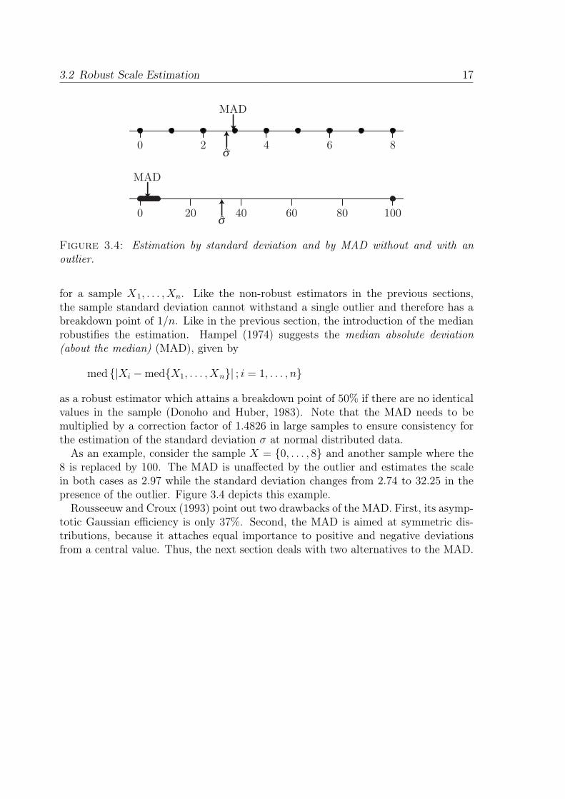
Figure 3.4: Estimation by standard deviation and by MAD without and with anoutlier.

for a sample X1, . . . , Xn. Like the non-robust estimators in the previous sections,the sample standard deviation cannot withstand a single outlier and therefore has abreakdown point of 1/n. Like in the previous section, the introduction of the medianrobustifies the estimation. Hampel (1974) suggests the median absolute deviation(about the median) (MAD), given by

med |Xi −medX1, . . . , Xn| ; i = 1, . . . , n

as a robust estimator which attains a breakdown point of 50% if there are no identicalvalues in the sample (Donoho and Huber, 1983). Note that the MAD needs to bemultiplied by a correction factor of 1.4826 in large samples to ensure consistency forthe estimation of the standard deviation σ at normal distributed data.

As an example, consider the sample X = 0, . . . , 8 and another sample where the8 is replaced by 100. The MAD is unaffected by the outlier and estimates the scalein both cases as 2.97 while the standard deviation changes from 2.74 to 32.25 in thepresence of the outlier. Figure 3.4 depicts this example.

Rousseeuw and Croux (1993) point out two drawbacks of the MAD. First, its asymp-totic Gaussian efficiency is only 37%. Second, the MAD is aimed at symmetric dis-tributions, because it attaches equal importance to positive and negative deviationsfrom a central value. Thus, the next section deals with two alternatives to the MAD.

18 3 Preliminaries

4 Online Computation of TwoEstimators of Scale

In the previous chapter, we encountered the MAD scale estimator. The MAD has asimple explicit formula, only needs O(n) computation time, and is very robust. Onthe other hand, its low Gaussian efficiency and the fact that it is aimed at symmetricdistributions are drawbacks. Rousseeuw and Croux (1993) propose two alternativescalled Sn and Qn that use order statistics (see Definition 3.2).

Definition 4.1. Let X1, . . . , Xn be a sample of size n.

1. The scale estimator Sn is defined as

Sn = c ·med med |Xi −Xj| ; j = 1, . . . , n ; i = 1, . . . , n .

2. The scale estimator Qn is defined as

Qn = c · |Xi −Xj| ; i < j(k) with k =

(bn/2c+ 1

2

).

The factor c is a consistency factor which is typically different for Sn and Qn.

Like the MAD, Sn and Qn typically need to be multiplied by a correction factor.When we want to ensure consistency for the estimation of the standard deviation σat normal distributed data, this factor is 1.1926 for the Sn and 2.2219 for the Qn inlarge samples (Rousseeuw and Croux, 1993). Sn and Qn can attain the same optimalbreakdown point as the MAD, but the asymptotic Gaussian efficiency of Sn and Qn is58% and 82%, respectively (Rousseeuw and Croux, 1993). This is superior to the 37%of the MAD. In addition, Sn and Qn do not presuppose a symmetric distribution. Thecomputation time needed is O (n log n) for both (Croux and Rousseeuw, 1992). This isasymptotically optimal for Qn, because—as we will see later—computing Qn is equiv-alent to a problem described in Johnson and Kashdan (1978) that needs Ω (n log n)time. For Sn no better lower bound than the trivial bound Ω (n) for median com-putation (Blum et al., 1973) is known. Our focus in this thesis is on efficient onlinecomputation of these estimators.

19

20 4 Online Computation of Two Estimators of Scale

0 1 2 3 4

1.0

0.0

1.0

2.0

time (sec)

hea

rt a

ctiv

ity (

mV

)

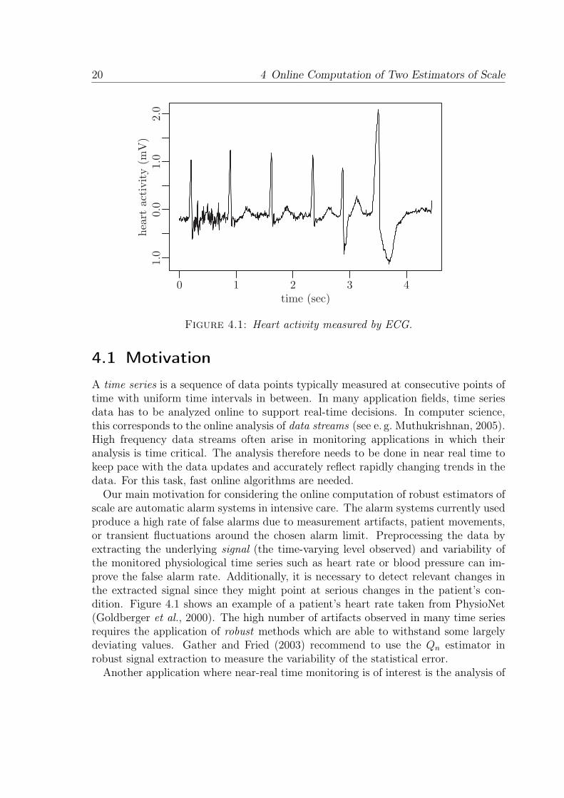
Figure 4.1: Heart activity measured by ECG.

4.1 Motivation

A time series is a sequence of data points typically measured at consecutive points oftime with uniform time intervals in between. In many application fields, time seriesdata has to be analyzed online to support real-time decisions. In computer science,this corresponds to the online analysis of data streams (see e. g. Muthukrishnan, 2005).High frequency data streams often arise in monitoring applications in which theiranalysis is time critical. The analysis therefore needs to be done in near real time tokeep pace with the data updates and accurately reflect rapidly changing trends in thedata. For this task, fast online algorithms are needed.

Our main motivation for considering the online computation of robust estimators ofscale are automatic alarm systems in intensive care. The alarm systems currently usedproduce a high rate of false alarms due to measurement artifacts, patient movements,or transient fluctuations around the chosen alarm limit. Preprocessing the data byextracting the underlying signal (the time-varying level observed) and variability ofthe monitored physiological time series such as heart rate or blood pressure can im-prove the false alarm rate. Additionally, it is necessary to detect relevant changes inthe extracted signal since they might point at serious changes in the patient’s con-dition. Figure 4.1 shows an example of a patient’s heart rate taken from PhysioNet(Goldberger et al., 2000). The high number of artifacts observed in many time seriesrequires the application of robust methods which are able to withstand some largelydeviating values. Gather and Fried (2003) recommend to use the Qn estimator inrobust signal extraction to measure the variability of the statistical error.

Another application where near-real time monitoring is of interest is the analysis of

4.2 Online Computation with Moving Windows 21

financial data. High frequency data are especially susceptible to errors as for examplestated by Brownlees and Gallo (2006):

The higher the velocity in trading, the higher the probability that someerror will be committed in reporting trading information.

In the financial context, we need preprocessing procedures for tasks like automaticdata cleaning and outlier detection. Non-robust estimators can be strongly misledby outliers. Preprocessing the data with robust methods has the advantage that therobust analysis resists isolated outliers and patches of outlying values. Robust scaleestimators allow us to extract possibly time-varying volatilities (the standard deviationof returns for a given financial parameter, for example a stock market index) in thepresence of outliers, see Gather and Fried (2003) and Gelper et al. (2009).

Further online applications of robust scale estimators include the estimation of au-tocorrelations within the process (Ma and Genton, 2000) and the standardization oftest statistics (Fried, 2007).

4.2 Online Computation with Moving Windows

To analyze the scale of an observed time series x1, . . . , xN online, we apply the scaleestimator at each time point t to a time window of length n ≤ N , which contains theobservations xt−n+1, . . . , xt. Instead of calculating the estimate for each window fromscratch, we use an online algorithm. This means that for each move of the window fromt to t+1 all stored information concerning the oldest observation xt−n+1 is deleted andnew information concerning the incoming observation xt+1 is inserted. Insertions anddeletions are called updates. Note that the online algorithms we propose in the nextsections are not restricted to moving time windows; they can also handle arbitrarysequences of deletions and insertions of data points.

When dealing with online algorithms, dynamic data structures are helpful. Thestandard operations that a data structure storing a multiset S of elements has to offeraccording to Cormen et al. (2001) include

1. Search(S, x), which searches for x in S,

2. Insert(S, x), which inserts x into S,

3. Delete(S, x), which deletes x from S.

Depending on the data structure and the specific requirements, x could be an elementfor the data structure, the key of an element, or a pointer to an element. An additionaloperation we will need is Rank(S, x), which gives the rank of x in S, i. e. the position ofx in sorted S. For the first algorithm, we will need fast insertion, deletion, searchingand ranking of an element. Every balanced binary search tree guarantees insertion,


deletion, and searching in time O(log n). The rank of an element may also be queriedin O(log n) if we store ranking information in each node of the search tree (see e. g.Knuth, 1973 or Cormen et al., 2001). We use AVL trees (Adel’son-Vel’skiı and Landis,1962) as balanced binary search trees. In the second algorithm, ranking will be moreimportant than insertion and deletion. For that case, we may use simple array or liststructures that allow rank queries in time O(1) but come with no better bound thanO(n) for insertion and deletion.

4.3 Computation of Qn

Qn is a high breakdown estimator with very good Gaussian efficiency and thereforea highly relevant robust scale estimator. Section 4.1 demonstrates that it is desirableto have fast online algorithms for computing this estimator. We present a fast onlinealgorithm based on the optimal offline algorithm in the following. As a first step, weshow that Qn may be computed by solving selection in the multiset X + Y .

Problem 4.1 (Selection in X + Y ).

Given: Two multisets X = x1, . . . , xn and Y = y1, . . . , yn and a parameter k ∈ N.

Goal: Compute

xi + yj;xi ∈ X and yj ∈ Y (k) .

For this problem, Johnson and Kashdan (1978) state an upper bound of O(n log n)and a lower bound of Ω(n+

√k log k) for computation in a decision tree. Problem 4.1

may be used to solve different problems from statistics. In the considered problems,k = Θ(n2) and thus the upper and the lower bound match.

Corollary 4.1. The complexity of computing the Hodges-Lehmann estimator (Hodgesand Lehmann, 1963) defined by

medXi +Xj; 1 ≤ i, j ≤ n2

for a sample X1, . . . , Xn is Θ (n log n).

Theorem 4.1 (Croux and Rousseeuw, 1992). The complexity of computing Qn for asample of size n is Θ (n log n).

Proof. Starting with Definition 4.1 we obtain

Qn = c · |Xi −Xj| ; i < j(k)= c · − |Xi −Xj| ; i > j ∪ |Xi −Xj| ; i = j ∪ |Xi −Xj| ; i < j((n

2)+n+k)

= c · Xi −Xj; 1 ≤ i, j ≤ n((n2)+n+k) .

4.3 Computation of Qn 23

x(1) + y(1) · · · x(1) + y(j−1) x(1) + y(j) x(1) + y(j+1) · · · x(1) + y(n)

x(i−1) + y(1) · · · x(i−1) + y(j−1) x(i−1) + y(j) x(i−1) + y(j+1) · · · x(i−1) + y(n)

x(i) + y(1) · · · x(i) + y(j−1) x(i) + y(j) x(i) + y(j+1) · · · x(i) + y(n)

x(i+1) + y(1) · · · x(i+1) + y(j−1) x(i+1) + y(j) x(i+1) + y(j+1) · · · x(i+1) + y(n)

x(n) + y(1) · · · x(n) + y(j−1) x(n) + y(j) x(n) + y(j+1) · · · x(n) + y(n)

···

···

···

···

···

···

···

···

···

···

···

···

· · ·

· · ·

≤≤

Figure 4.2: Regions in the matrix M with definitely smaller or certainly greatervalues than x(i) + y(i).

This corresponds to Problem 4.1 for a multiset of type X + (−X) and the parameter(n2

)+ n+ k.

Note that there are further estimators, e. g. the medcouple (Brys et al., 2004), thatmay be computed with an algorithm for Problem 4.1.

4.3.1 Offline Computation

In Theorem 4.1, we saw that it is possible to compute the Qn by solving Problem 4.1.This is why we only consider Problem 4.1 in the following. Shamos (1976) providesan algorithm he devised with Jefferson and Tarjan for computing

medxi + yj;xi ∈ X and yj ∈ Y

in O(n log n) and also states a lower bound of Ω(n log n) communicated by Tarjan.Johnson and Mizoguchi (1978) adapt this algorithm to compute an arbitrary order

statistic, i. e. to solve Problem 4.1. It is convenient to visualize the algorithm ofJohnson and Mizoguchi working on a partially sorted matrix M = (mij) with mij =x(i) + y(j), although M is of course never constructed. Recall that x(1) ≤ . . . ≤ x(n)

and y(1) ≤ . . . ≤ y(n) denote the elements of X and Y ordered according to size. Thus,the matrix M has monotonicity in the rows and columns, i. e. mij = x(i) + y(j) ≤x(i) + y(`) = mi` and mji = x(j) + y(i) ≤ x(`) + y(i) = m`i for j ≤ `. The algorithmuses this monotonicity to compute the desired order statistic (see Figure 4.2 for anexample of this monotonicity).

Algorithm 4.1 sketches the algorithm of Johnson and Mizoguchi (1978). Steps 1–3take time O (n log n) because of the sorting of X and Y . No computation is done inline 2. If the element in line 5 is carefully selected which takes time O (n) (we omit thedetails), the while loop will run O(log n) times. Line 10 comprises a selection problemwhich can be carried out in time O (n) (see e. g. Cormen et al., 2001).


Algorithm 4.1: Sketch of the algorithm of Johnson and Mizoguchi (1978)Input: Multisets X = x1, . . . , xn and Y = y1, . . . , yn, parameter kOutput: The kth order statistic of X + YSort X and Y1

Let M = (mij) with mij = x(i) + y(j) denote the partially sorted matrix of X + Y2

Set c := n23

while c > n do4

Select an element m of M that is still a candidate for the kth order statistic5

Determine regions in the matrix definitely smaller or certainly greater than m6

Exclude all parts of these regions that cannot contain the sought order7

statisticUpdate c, which denotes the number of matrix elements still under8

considerationend9

Determine directly which of the remaining elements of M is the kth order10

statistic of X + Yreturn the determined order statistic11

4.3.2 Online Computation

The offline algorithm has optimal running time. In this section, we try to be fasterfor online computation and present a new algorithm. Online algorithms for a problemsimilar to computing Qn exist. Bespamyatnikh (1998) states an online algorithm forcomputing

|xi − xj| ; i < j(k) with k = 1 (4.1)

that achieves O(log n) per update step. This is optimal, because the lower bound foroffline compuataion is Ω(n log n) (Preparata and Shamos, 1985). Note, that (4.1) isthe well known problem of computing the minimal distance between two numbers ina set. In an earlier work on minimal distance computation, Smid (1991) suggests touse a buffer of possible solutions to obtain an online algorithm for this problem. Thebuffer contains the elements |xi − xj| ; i < j(1) , |xi − xj| ; i < j(2) , . . . and enablesfast updates because the new minimal distance after an update is likely to be found inthe buffer. However, the computation of the Qn estimator requires larger k. Hence, wegeneralize the idea of using a buffer to arbitrary values of k in the following, becauseit is easy to implement and achieves a good running time in practice. The resultingalgorithm will have a worst case amortized time per update that is the same as forthe offline algorithm. However, we show that our algorithm runs substantially fasterunder certain data assumptions and also runs faster for many data sets not fulfillingthese assumptions.

Algorithm 4.1 may easily be extended to compute a buffer B of s matrix elements


m(k−b(s−1)/2c), . . . ,m(k+bs/2c) from M next to the solution m(k). We discuss the sizes of the buffer B later. We first describe the framework of the online algorithm inAlgorithm 4.2 and later give the details on how to insert and delete elements.

Algorithm 4.2: Moving window selection in X + Y

Input: Samples X and Y , parameter k, window width n, buffer size sOutput: The kth order statistic of each window in X + YSet Xw := x1, . . . , xn and Yw := y1, . . . , yn1

Compute the kth order statistic of Xw + Yw and a buffer B of size s offline2

for t← n to |X| − 1 do3

Call Insert(xt+1, Xw, Yw, B) and Delete(xt−n+1, Xw, Yw, B)4

Call Insert(yt+1, Yw, Xw, B) and Delete(yt−n+1, Y w, Xw, B)5

if Delete(yt−n+1, Y w, B) returned that the kth order statistic of6

xt−n+1, . . . , xt+1+ yt−n+1, . . . , yt+1 is in B thenDetermine the kth order statistic directly7

else8

Recalculate the kth order statistic and the buffer B offline9

end10

end11

return the determined order statistics12

To speed up online computation, we ensure fast insertion and deletion and fewof the recalculations done in line 9. To achieve this, we use indexed AVL trees asthe main data structure. As mentioned in Section 4.2, inserting, deleting, findingand determining the rank of an element takes O(log n) time in this data structure.Moreover—in the data structure we use—every element in the balanced tree has twopointers allowing access to the element pointed at in time O(1). In detail, we storeX, Y and B in separate balanced trees and manage the following pointers:

1. Each element mij = x(i) + y(j) in the buffer B gets two pointers: one pointer tox(i) ∈ X and one pointer to y(j) ∈ Y .

2. Each element x(i) in X (corresponding to elements in the ith row of M) gets onepointer to the smallest and one pointer to the largest element such that mij ∈ Bfor 1 ≤ j ≤ n.

3. Each element y(j) in Y (corresponding to elements in the jth column of M) getsone pointer to the smallest and one pointer to the largest element such thatmij ∈ B for 1 ≤ i ≤ n.

Figure 4.3 shows an example for these pointers where the arrows with solid tips markthe pointers of a matrix element and the “”-tips mark the pointers to the smallestand largest element. Note that the buffer may of course be much larger and the


x(1) + y(1) · · · x(1) + y(j) x(1) + y(j+1) · · · x(1) + y(n)

x(i−1) + y(1) · · · x(i−1) + y(j) x(i−1) + y(j+1) · · · x(i−1) + y(n)

x(i) + y(1) · · · x(i) + y(j) x(i) + y(j+1) · · · x(i) + y(n)

x(i+1) +y(1) · · · x(i+1) + y(j) x(i+1) + y(j+1) · · · x(i+1) + y(n)

x(n) + y(1) · · · x(n) + y(j) x(n) + y(j+1) · · · x(n) + y(n)

···

···

···

···

···

···

···

···

···

···

· · ·

· · ·

x(1)

x(i−1)

x(i)

x(i+1)

x(n)

y(1) · · · y(j) y(j+1) · · · y(n)···

···

x(1)

x(i−1)

x(i)

x(i+1)

x(n)

···

···

y(1) · · · y(j) y(j+1) · · · y(n)

Figure 4.3: Example for the pointer structure.

pointers of elements in X and Y only point to the boundaries of the buffer. Theoffline Algorithm 4.1 may easily be extended to return this data structure and thebuffer without using more time than O (n log n).

The following procedures Insert and Delete handle insertions into and deletionsfrom X. Insertions into and deletions from Y work analogously with slightly differentprocedures.

Procedure Insert(xins, sample X, sample Y , buffer B)Input: Element to insert xins, sample X, sample Y , buffer BOutput: changed sample X and buffer B, information whether the kth element

of X + Y is still in B// Compute all elements in the new matrix row defined by xins that

belong into the bufferDetermine the smallest element bs and the greatest element bg in B1

Determine with a binary search the smallest j such that xins + y(j) ≥ bs and the2

greatest ` such that xins + y(`) ≤ bgCompute all elements Bm := xins + y(m) | j ≤ m ≤ `3

// Insert these elements into the buffer and xins into XInsert the elements in Bm into the buffer B4

Insert xins into X5

// Update the data structureUpdate pointers to and from the inserted elements accordingly6

Compute the new position of the kth element of X + Y in B by counting how7

many smaller and how many greater elements were insertedreturn X, B and whether the kth element of X + Y is still in B8

The basic operations in our data structure need time O(log n), following a pointerneeds time O(1). These time bounds apply for most of the algorithm steps. The binary


Procedure Delete(xdel, sample X, sample Y , buffer B)Input: Element to delete xdel, sample X, sample Y , buffer BOutput: changed sample X and buffer B, information whether the kth element

of X + Y is still in B// Get the element to delete and its rank in the data structureSearch in X for xdel1

Determine the rank i of xdel and the elements bs and bg pointed at2

// Determine all elements in the matrix row defined by xdel that arein the buffer

Determine y(j) and y(`) with the help of the pointers of bs and bg such that3

bs = x(i) + y(j) and bg = x(i) + y(`)

Find Bm := x(i) + y(m) ∈ B | j ≤ m ≤ `4

// Delete these elements from the buffer and xdel from XDelete the elements in Bm from the buffer B5

Delete xdel from X6

// Update the data structureUpdate the affected pointers accordingly7

Compute the new position of the kth element of X + Y in B by counting how8

many smaller and how many greater elements were deletedreturn X, B and whether the kth element of X + Y is still in B9

search in line 2 of Insert needs time O (log n). The only operations needing moretime than O (log n) are the ones concerning the set Bm. Thus, we see that Insertand Delete need a maximum of O(|Bm| · log n) time for insertion and deletion, whereBm is defined as in the procedures. It is possible to introduce bounds on the size ofB and to recompute B if these bounds are violated to limit the space requirement ofthe online algorithm. We will use a bound of O(n) in the following. For arbitrarysequences of insertions and deletions, the size of B can vary more and we may have torecompute the buffer more often than for moving time windows. To assess the runningtime we have to consider first the number of elements in the buffer that depend onthe inserted or deleted observation, i. e. the typical size of Bm.

Theorem 4.2. For a constant signal with identically distributed noise variables theexpected time needed for insertion or deletion of data points is O(log n).

Proof. For a constant signal with identically distributed error terms, data pointsare exchangeable in the sense that each rank of a data point in the set of all ndata points occurs with equal probability 1/n. Assume without loss of generalitythat we only insert into and delete from X. We define random variables Dx(i)

=∣∣x(i) + y(j) ∈ B; 1 ≤ j ≤ n∣∣ for x(i) ∈ X that describe the number of buffer elements

in the buffer B depending on x(i). As a first step, we consider the deletion of xdel from


X with equiprobable ranks. The expected value E (Dxdel) is given by

E (Dxdel) =

1

nDx(1)

+ . . .+1

nDx(n)

=1

n

n∑i=1

Dx(i)=

1

n|B| .

When we insert an element xins into X, it is inserted between two elements x(i) andx(i+1). Because of the monotonicity of the matrix M , the number of buffer elementsdepending on xins after its insertion cannot be greater than Dx(i) +Dx(i+1). Let Sx(i)

=Dx(i) +Dx(i+1) with Sx(0) = Dx(1) and Sx(n) = Dx(n). We consider the insertion of xins

with equiprobable ranks. The expected value E (Dxins) is given by

E (Dxins) ≤ 1

n+ 1Sx(0)

+ . . .+1

n+ 1Sx(n)

=2

n+ 1

n∑i=1

Dx(i)=

2

n+ 1|B| .

The size of the buffer |B| is O (n). Thus, E (Dxdel) and E (Dxins

) are O(1) and we expectto spend O(E (Dxins

) log n) = O(log n) time for the insertion and O(E (Dxdel) log n) =

O(log n) for the deletion of a data point.

At times, we have to recompute the buffer which needs O(n log n) time and increasesthe amortized time per update. The frequency of recomputations depends on howmuch the kth element of X + Y may move in the buffer. With equiprobable ranks asin Theorem 4.2, the expected position of the kth element in the buffer after a deletionand a subsequent insertion is the same as before the deletion and the insertion. Thus,we expect to recompute the buffer very rarely.

The next section contains running time simulations for data that fulfills the assump-tions of Theorem 4.2 and for more complex data situations.

4.3.3 Running Time Simulations

To demonstrate the good performance of the new online algorithm in practice, weconduct running time simulations for online computation of the Qn estimator. We usethree different simulated time series and a real time series and consider the extractionof possibly time-varying volatilities.

The basis of the first time series (depicted in Figure 4.4) is a benchmark modelwhich is commonly used to estimate and predict volatility processes. This benchmarkmodel is given by the GARCH(1,1) model proposed by Bollerslev (1986)

Xt = σtεt, t ∈ Z ,

where εt ∼ N (0, 1) is an error term and σt is a time-varying volatility coefficient.More precisely, the conditional variance σ2

t = Var(Xt|Xt−1, Xt−2, . . .) is given by

σ2t = α0 + α1X

2t−1 + β1σ

2t−1


0 200 400 600 800 1000

20

24

Simulated GARCH(1,1) Process

time

seri

es

0 200 400 600 800 1000

0.8

1.2

1.6

Online Scale Estimation (n = 50)

time

scal

e

true σt

Qn

Figure 4.4: Simulated GARCH(1,1) series (left) and estimated volatilities (right).

0 200 400 600 800 1000

020

4

Piecewise Constant Variance

time

seri

es

0 200 400 600 800 1000

12

34

56

78


time

scal

e

true σt

Qn

Figure 4.5: Time series with piecewise constant variance (left) and estimated volatil-ities (right).

with parameters α0 > 0 and α1, β1 ≥ 0. Note that GARCH(1,1) processes with therestriction α1 + β1 < 1 are stationary and thus fulfill the assumption of Theorem 4.2.Figure 4.4 shows such a time series of length N = 1000 generated from a GARCH(1,1)model with coefficients α0 = 0.1, α1 = 0.1 and β1 = 0.8. Additionally, we see thevolatilities estimated by the Qn when using a window width of n = 50. Qn tracks thevolatility rather well. However, since for online analyses only past observations aretaken into account, a sudden increase or decrease in volatility is traced with some timedelay. This time delay is relatively small for the Qn leading to a smooth sequence ofestimates.

The second time series of length N = 1000 (shown in Figure 4.5) possesses a piece-wise constant volatility σt, which equals 1, 5, 1, 3, and 5, in time periods of length 200,250, 150, 250, and 150, respectively. Such models with piecewise constant volatility


Simulated AR(1) Process

time

seri

es

0 200 400 600 800 1000

05

10

0 200 400 600 800 1000

1.0

2.0

3.0


time

scal

e

true σt

Qn

Figure 4.6: Time series with piecewise constant level plus additive noise generatedfrom an AR(1) model (left) and estimated volatilities (right).

0.

50.

0

Daily returns of Bayer AG stocks

retu

rns

1960 1975 1990 2005

0.01

0.02

0.03

Online Scale Estimation (n = 250)sc

ale

1960 1975 1990 2005

Figure 4.7: Daily returns of Bayer AG stocks between January 4, 1960 and July 17,2007 (left) and estimated volatilities (right).

are suggested by Mercurio and Spokoiny (2004) to approximate financial time series.The simulated time series shown in Figure 4.5 consists of independent normal errorswith standard deviations given above, plus 10% positive additive outliers of size 6σtat random time points. The Qn can cope with the outliers and yields a stable scaleestimation over time.

The third example (depicted in Figure 4.6) consists of a time series of length N =1000 with positive level shifts of size 1, 3, and 5 at times 201, 401, 601, respectively,and a negative level shift of size −9 at time 801. Thus, the observations vary aroundthe values 0, 1, 4, 9, and 0. The errors are generated from an AR(1) model which isdefined by

Xt = ϕXt−1 + εt t ∈ Z ,

where εt ∼ N (0, 1). The variance in this model is σ2t = 1/ (1− ϕ2), which is indepen-


0 1000 2000 3000 4000 5000

0.00

00.

004

0.00

80.

012

window width

runn

ing

tim

e (s

ec)

Offline algorithmAR(1) with shiftsPiecewise constantBayerGARCH(1,1)

Figure 4.8: Running time needed for the online analyses of the four considered datasituations in comparison to the offline algorithm for different window widths.

dent of t, see e. g. Brockwell and Davis (2002). Figure 4.6 shows a time series simulatedaccording to the settings above with ϕ = 0.4. We observe that the estimations lie closeto the true value of σt but that shifts cause strong biases. Larger shifts have largerimpact on the online scale estimation.

The fourth time series is a real data set depicted in Figure 4.7. It consists of the re-turns (the first differences of the logarithms of daily closing prices) of Bayer AG stocksbetween January 4, 1960 and July 17, 2007. The variability of these returns is impor-tant for assessing derivate finance products like options. Because of unexpected eventslike regulatory changes, technological advances, natural catastrophes or accidents, fi-nancial time series can contain arbitrarily large outliers. We therefore should apply arobust scale estimator to evaluate the (local) variability. In this particular case, thisis especially reasonable since the underlying prices are not adjusted for dividends andsplits. Figure 4.7 shows that the time series obviously contains periods of increased ordecreased variability as well as some outliers, a few of them being rather large. It alsoshows the estimates of the time-varying volatility obtained from applying the Qn toa moving window of width n = 250 corresponding to the commonly assumed numberof trading days within one year. Qn resists the outliers well since there are only a fewvery large ones.

On these four data sets, we analyze the average time needed for an update of Qn

when using windows of width 50 ≤ n ≤ 5000 (shown in Figure 4.8). For windows withwidth n < 50, the difference in running times is too small for accurate measurement,i. e. smaller than 0.1ms, and there is little difference in using the offline or the online


column

row

200

400

600

800

200 400 600 800

200 400 600 800

200

400

600

800

0

100

200

300

400

500

600

700

800

Figure 4.9: Positions of the buffer B in the matrix M for the GARCH(1, 1) data(top left), the model with piecewise constant volatility (top right), the Bayer AG data(bottom left), and the data with level shifts and AR(1) errors (bottom right).

algorithm.In order to get similar situations for all window widths, we generate new data sets

for each n. For the GARCH model we simulate data sets of size N = n + 2500. Forthe time series with a piecewise constant σt and the AR(1) process with level shiftswe set the length of each part to n+ 500.

Figure 4.8 illustrates a very good online running time for the GARCH(1,1) series,as could be expected from Theorem 4.2. In case of the real data example and the dataset with piecewise constant variances, we also notice a considerable improvement inrunning time. The improvement for the time series with level shifts is not as good.The offline computation time is nearly the same for all data sets. Therefore, we includeonly the overall average of the offline computation times for each window width forcomparison.

To gain some insight into the different runtimes needed, we analyze the position ofthe buffer B in the matrix M over time when performing 1000 updates with a windowof size 1000. We see in Figure 4.9 that the more complex data situations result in amore spread buffer and therefore more computation time per update.

4.4 Computation of Sn 33

4.4 Computation of Sn

So far, we compared robust scale estimators in terms of breakdown point and Gaussianefficiency. Under these criteria, Qn is superior to Sn. However, these properties areasymptotic and not advantageous in all cases. In fact, Rousseeuw and Croux (1993)recommend using Sn for most applications. Thus, computing Sn fast online is also ofhigh interest. Similar to Section 4.3, we start with a description of the existing offlinealgorithm and then present a faster online algorithm.

4.4.1 Offline Computation

As a first step, we formulate the computation of Sn as an algorithmic problem. Crouxand Rousseeuw (1992) use a slightly different definition of Sn for computation.

Problem 4.2 (Computation of Sn).

Given: A sample X1, . . . , Xn and a correction factor c.

Goal: Compute|Xi −Xj| ; j 6= i(b(n+1)/2c) ; i = 1, . . . , n

(b(n+1)/2c)

and multiply it with the correction factor c.

Croux and Rousseeuw (1992) also describe an algorithm to compute Sn that needstime O(n log n).

Theorem 4.3 (Croux and Rousseeuw, 1992). Computing Sn for a sample X1, . . . , Xn

is possible in time O(n log n).

Proof. In a first step, we sort the sample in time O(n log n). We may compute theinner order statistics

|Xi −Xj| ; j 6= i(b(n+1)/2c)

of Problem 4.2 for each i = 1, . . . , n by computing(X(i) −X(i−1), . . . , X(i) −X(1)

∪X(i+1) −X(i), . . . , X(n) −X(i)

)(b(n+1)/2c) .

Note that we do not need to compute all values of these sorted sets. Shamos (1976)presents an algorithm by Jefferson to compute the common median (or b(n+ 1)/2cthorder statistic in this case) of two sorted sets in time O(log n). This has to be donen times and afterwards, the b(n+ 1)/2cth order statistic of the n computed elementshas to be computed. Finally, the result is multiplied with the correction factor c. Noneof these steps takes more time than O(n log n).


≤≤≤ ≤

Figure 4.10: Illustration of L1, G1, L2, and G2.

4.4.2 Online Computation

To our knowledge, there is no online algorithm for Sn, yet. Fried et al. (2006) presentan online algorithm for the repeated median estimator , which also contains an innerand an outer median and therefore bears similarity to the Sn. The online algorithm forthe repeated median needs time O (n) per update. However, we state a much simpleralgorithm for the Sn which also needs time O (n) per update.

To construct this online algorithm, we review the offline algorithm sketched in theproof of Theorem 4.3. The offline algorithm works on multisets

C (i) =X(i) −X(i−1), . . . , X(i) −X(1)

∪X(i+1) −X(i), . . . , X(n) −X(i)

.

The two sets in C (i) are sorted in increasing order. The algorithm presented byShamos (1976) that computes the common b(n+ 1)/2cth order statistic of these setsC (i) returns the information which elements are smaller or equal and which elementsare greater or equal than the computed value. Thus, it is convenient to imaginethat

X(i) −X(i−1), . . . , X(i) −X(1)

and

X(i+1) −X(i), . . . , X(n) −X(i)

are split into

halves by the algorithm.We can easily adapt the offline algorithm to return values m(i) that implicitly define

multisets reflecting this split. The multiset L1 contains the elements smaller or equalthan C(i)b(n+1)/2c and G1 contains the elements greater or equal than C(i)b(n+1)/2c inthe case that C(i)b(n+1)/2c is in the first set

X(i) −X(i−1), . . . , X(i) −X(1)

. L2 and G2

comprise the case that C(i)b(n+1)/2c is in the second setX(i+1) −X(i), . . . , X(n) −X(i)

.

Figure 4.10 illustrates this idea. More precisely, the multisets L1, G1, L2, and G2 aredefined as

L1(m(i)) =X(i) −X(i−1), . . . , X(i) −X(m(i)+1)

∪

X(i+1) −X(i), . . . , X(m(i)+b(n+1)/2c) −X(i)

G1(m(i)) =

X(i) −X(m(i)−1), . . . , X(i) −X(1)

∪

X(m(i)+b(n+1)/2c+1) −X(i), . . . , X(n) −X(i)

L2(m(i)) =

X(i) −X(i−1), . . . , X(i) −X(m(i)−b(n+1)/2c)

∪

X(i+1) −X(i), . . . , X(m(i)−1) −X(i)

G2(m(i)) =

X(i) −X(m(i)−b(n+1)/2c−1), . . . , X(i) −X(1)

∪

X(m(i)+1) −X(i), . . . , X(n) −X(i)


such that

∃j ∈ 1, 2 : (|Lj(m(i))| = b(n+ 1)/2c − 1) ∧(∀s ∈ Lj(m(i)), g ∈ Gj(m(i)) : s ≤

∣∣X(i) −X(m(i))

∣∣ ≤ g).

It is possible to let the algorithm return the values m (i), because∣∣X(i) −X(m(i))

∣∣ iswhat the original offline algorithm computes as C(i)b(n+1)/2c. The algorithm only hasto report the position of

∣∣X(i) −X(m(i))

∣∣ in C(i) instead of its value. After executingsuch an adapted offline algorithm on a sample X1, . . . , Xn all m(i) are known for eachi with 1 ≤ i ≤ n. This leads to the possibility of a fast update for the b(n+ 1)/2cthorder statistics. We will see, that it is possible to update each of the inner orderstatistics |Xi −Xj| ; j 6= i(b(n+1)/2c) in time O(1) with this information. In principle,only three cases can occur: the order statistic does not change, the biggest elementin Lj (m(i)) takes its place, or the smallest element in Gj (m(i)) takes its place. Theupdate of the outer order statistic then takes time O (n) leading to time O (n) perupdate. Let us first look at the framework of the online algorithm working on theobserved values x1, . . . , xN of a sample X1, . . . , XN in Algorithm 4.5.

Algorithm 4.5: Moving window computation of SnInput: observed sample X = x1, . . . , xN, window width nOutput: Scale estimate Sn for each window in XSet Xw := x1, . . . , xn1

Compute Sn of Xw offline2

Store the returned Sn value in sn and the returned m (i) values in m3

for t← n to |X| − 1 do4

Call Insert(xt+1, Xw, m)5

Call Delete(xt−n+1, Xw, m)6

Calculate ∣∣x(i) − xm(i)

∣∣ ; 1 ≤ i ≤ |X|(b(n+1)/2c)7

Store the calculated value in st+18

end9

return the determined scale estimates sn, . . . , sN10

To achieve the desired runtime, we need a data structure S for Xw = x1, . . . , xn thatallows the operations Rank(S, xi) and Search(S, xi) for an element xi in time O (1) ifthe index i of either xi or x(i) is known, but may take up to O (n) time for Insert(S, xi)and Delete(S, xi), respectively. As the first window Xw in Algorithm 4.5 gets sortedin the offline algorithm, it suffices to use two arrays (one sorted by index, one sortedby rank) with a function mapping between index and rank of an element.

As a first observation, we see that the time needed to update the Sn value after aninsertion and a deletion is O(n) in Algorithm 4.5 because selecting the b(n+ 1)/2cthorder statistic of

∣∣X(i) −Xm(i)

∣∣ ; 1 ≤ i ≤ |X| determines the runtime. To obtain theoverall update time, we have to look at the time needed for insertion and deletion.


We confine insertion and deletion to the case where∣∣X(i) −Xm(i)

∣∣ = X(i)−Xm(i) (thesearched element is in the left part of C(i)) because the other case works analogously.

Procedure Insert(xins, sample X, m)Input: Element to insert xins, sample X, mOutput: changed sample X, changed m// Desired order statistic before and after the insertionk = b(|X|+ 1)/2c, k′ = b(|X|+ 1 + 1)/2c1

Insert xins into X and determine p such that x(p) = xins2

// Adapt the indices in m to the change caused by insertionfor i← 1 to |X| − 1 do if m(i) ≥ p then m(i) = m(i) + 13

for i← |X| downto p+ 1 do m(i) = m(i− 1)4

Compute m(p) by computing C(p)b(n+1)/2c5

foreach i ∈ 1, . . . , |X| \ p do6

// Insertion into L1(m(i)) and no change in k

if∣∣x(i) − x(p)

∣∣ ≤ x(i) − x(m(i)) and m(i) + k + 1 ≥ p > m(i) and k = k′ then7

if m(i) + k + 1 > |X| or8 (m(i) + 1 < i and x(i) − x(m(i)+1) ≥ x(m(i)+k+1) − x(i)

)then

m(i) = m(i) + 19

else10

m(i) = m(i) + k + 111

end12

// Insertion into G1(m(i)) and a change in k13

else if∣∣x(i) − x(p)

∣∣ ≥ x(i) − x(m(i)) and (p < m(i) or p > m(i) + k) and k 6= k′14

thenif m(i) + k + 1 > |X| or15 (m(i)− 1 < i and x(i) − x(m(i)−1) ≤ x(m(i)+k+1) − x(i)

)then

m(i) = m(i)− 116

else17

m(i) = m(i) + k + 118

end19

end20

end21

return X, m22


Procedure Delete(xdel, sample X, m)Input: Element to delete xdel, sample X, mOutput: changed sample X, changed m// Desired order statistic before and after the deletionk = b(|X|+ 1)/2c, k′ = b(|X| − 1 + 1)/2c1

Determine p such that x(p) = xdel and delete xdel from X2

// Adapt the indices in m to the change caused by deletion and markthe cases where the element m(i) points at was deleted

for i← 1 to |X|+ 1 do3

if m(i) = p then del(i) = true else del(i) = false4

if m(i) > p then m(i) = m(i)− 15

end6

for i← p to |X| do m(i) = m(i+ 1)7

foreach i ∈ 1, . . . , |X| do8

// Deletion of x(i) − x(m(i)) or from L1(m(i)) and no change in kif (m(i) + k ≥ p > m(i) or del(i)) and k = k′ then9

if m(i) + k > |X| or(m(i)− 1 < i and x(i) − x(m(i)−1) ≥ x(m(i)+k) − x(i)

)10

thenm(i) = m(i)− 111

else12

m(i) = m(i) + k13

end14

// Deletion of x(i) − x(m(i)) or from G1(m(i)) and a change in k15

else if (p ≤ m(i) or p > m(i) + k or del(i)) and k 6= k′ then16

if del(i) then m(i) = m(i)− 117

if m(i) + k > |X| or(m(i) + 1 < i and x(i) − x(m(i)+1) ≤ x(m(i)+k) − x(i)

)18

thenm(i) = m(i) + 119

else20

m(i) = m(i) + k21

end22

end23

end24

return X, m25


Theorem 4.4. The time needed to update an Sn scale estimation on a sample of sizen after an insertion or deletion is O(n).

Proof. In the first part of the proof, we show the correctness of Insert and Delete.In the second part, we consider the runtime.

Let X be the sample before insertion or deletion and let k = b(|X|+ 1)/2c, kins =b(|X|+ 1 + 1)/2c, and kdel = b(|X| − 1 + 1)/2c.Lines 2–4 of Insert ensure that m temporarily points to the same elements as

before, although some order statistics (indices) changed. Line 5 computes m for thenewly inserted value. Lines 6–21 contain the loop doing this for all other values. Lines7–12 handle the case, that the element x(p) − x(i) defined by the newly inserted valuebelongs into L1(m(i)) (the test is for m (i) + k + 1 ≥ p > m(i) and not m (i) +k ≥ p > m(i) because the additional element changes the ranks). If kins = k + 1,we have to do nothing because we already have one additional element in L1(m(i)).Otherwise, we have to search for maxL1(m(i)) which is clearly the same as maxx(i)−x(m(i)+1), x(m(i)+k+1) − x(i). Lines 14–20 handle insertion into G1(m(i)) analogously.

Lines 2–7 of Delete ensure that m temporarily points to the same elements asbefore, and marks when the element pointed at is deleted. Lines 8–24 contain theloop correcting the m values. Lines 9–14 handle the case, that an element was deletedfrom L1(m(i)). If kdel = k − 1, we have nothing to do. Otherwise, we have to searchfor minG1(m(i)), which is clearly the same as maxx(i) − x(m(i)−1), x(m(i)+k) − x(i)(x(m(i)+k) − x(i) is an element of G1(m(i)) and not of L1(m(i)) because one elementof L1(m(i)) was deleted). Lines 9–14 handle deletions from G1(m(i)) analogously. Aspecial case occurs, when the element originally pointed at by m(i) is deleted. Ifkdel = k we have to do the same as if deleting from L1(m(i)). Otherwise, we have tocare about the ranks. Decreasing the old value of m (i) and beyond that doing thesame as if deleting from G1(m(i)) handles this case correctly. Therefore, all cases arehandled correctly and Insert and Delete work correctly.The runtime is determined by the operations that select elements of X by rank.

In Insert and Delete this is done O(n) times. When we use the described datastructure, this needs time O (n). After Insert and Delete Algorithm 4.5 spendsO(n) time to update the Sn value. Thus, the overall time is as claimed.

5 Computing the Least QuartileDifference Estimator in the Plane

The main reason why Rousseeuw and Croux (1993) suggest Qn and Sn as alternativesto the MAD for robust scale estimation is their advantage in Gaussian efficiency.For the case of linear regression, we saw in Section 3.1 that the LMS estimator showsrobustness advantages over LAD and LS. However, the LMS also has the disadvantageof a low Gaussian efficiency, which is asymptotically 0% (Croux et al., 1994). Crouxet al. (1994) propose the least quartile difference estimator as an alternative.

Definition 5.1. The least quartile difference (LQD) estimates β0, ..., βp = βLQD of theregression parameters β0, ..., βp are given by

βLQD = minβ0,...,βp

|ri (β0, . . . , βp)− rj (β0, . . . , βp)| ; i < j(hp2 ) with hp =

⌊n+ p+ 2

2

⌋.

Note, that computing |ri (β0, . . . , βp)− rj (β0, . . . , βp)| ; i < j(hp2 ) corresponds to com-

puting the Qn estimator on residuals. The LQD is a high-breakdown method with abreakdown point of 50%, it has an asymptotic Gaussian efficiency of 67.1% and doesnot presuppose a symmetric distribution. An additional property is that the functionLQD minimizes does not depend on the intercept term. Taking a look at the defini-tion of a residual difference ri (β0, . . . , βp) − rj (β0, . . . , βp) (residuals were defined inDefinition 3.7) we see why this is the case. The residual difference of the estimatesβ0, ..., βp

ri − rj = yi − Yi −(yj − Yj

)= yi −

(β0 + β1xi1 + . . .+ βpxip

)− yj + β0 + β1xj1 + . . .+ βpxjp

= (yi − yj)− β1 (xi1 − xj1)− . . .− βp (xip − xjp) (5.1)

does not depend on β0. Therefore, the intercept of the LQD regression has to beestimated afterwards, e. g. by

medyi − (β1xi1 + . . .+ βpxip) | 1 ≤ i ≤ n .

Several algorithms exist for the LQD. In the following, we state results for the casep = 1, i. e. estimation in the plane. In their article, introducing the LQD estima-tor, Croux et al. (1994) propose to use the subset algorithm developed by Rousseeuw

39

40 5 Computing the Least Quartile Difference Estimator in the Plane

and Leroy (1987). The subset algorithm is based on examining subsets of the datapoints that determine local solutions, i. e. estimates β0, ..., βp that are not necessarilythe global solution. The

(h1

2

)th order statistic of the absolute residual differences of

a local solution can be computed in time O(n log n) as seen in Section 4.3.1. Crouxet al. (1994) propose to examine all O(n2) or alternatively just O(n) randomly chosen2-subsets of the data points, which needs overall time O(n3 log n) or O(n2 log n), re-spectively. However, the resulting algorithm is not exact because the global solutionis not necessarily determined by a 2-subset. The exact algorithm they propose needstime O(n5 log n). Another possibility to compute the LQD regression fit is to adaptLMS or least quantile of squares (LQS) algorithms. LQS is a generalization of LMS.

Definition 5.2. The least quantile of squares (LQS) estimates β0, ..., βp = βLQS of theregression parameters β0, ..., βp are given by

βLQS = minβ0,...,βp

r1 (β0, . . . , βp)2 , . . . , rn (β0, . . . , βp)

2(hp) with 1 ≤ hp ≤ n .

The adaption proposed by Croux et al. (1994) leads to a running time of O(n4), ifthe algorithms of Souvaine and Steele (1987) or Edelsbrunner and Souvaine (1990) forcomputing LMS in time O(n2) are used. Agulló (2002) proposes an approximationalgorithm for LQD, but only gives empirical running time results.

Due to the high computational effort needed when using common algorithms, theLQD is not widely used, yet. However, Dryden and Walker (1999) propose to use itfor object matching in biology and Mebane, Jr. and Sekhon (2004) use the LQD fitto detect outliers in vote counts.

5.1 The Concept of Geometric Duality

To construct a faster algorithm for LQD estimation, we utilize geometric duality.Classically, geometric duality is defined in the plane. Points in the plane and lines inthe plane are both described by two parameters. It is therefore possible to map a setof points to a set of lines, and vice versa, in a one-to-one manner. Such a mappingfrom a primal space to a dual space is called duality transform and typically preservescertain properties and relations existing in the primal space. It is widely believed,that it is easier to search for a point in an arrangement of lines, than to search for aline through a set of points. As a matter of fact, the data structures and algorithmsused in computational geometry strongly support that belief.

We concentrate on the version of geometric duality that Chazelle et al. (1985) pro-pose for solving geometrical problems. In particular, we state the formulation ofde Berg et al. (2008). Their geometric transform maps a primal point p = (β1, β0)to a dual line Tp : y = β1x − β0 and a primal line ` : y = β1x + β0 to a dual point

5.1 The Concept of Geometric Duality 41

x

y

1.510.50-0.5-1-1.5

32

10

-1-2

-3

x1.510.50-0.5-1-1.5

32

10

-1-2

-3

Primal Space Dual Space

Figure 5.1: Nine points and a line in primal space and the corresponding dual space.

T` = (β1,−β0). The merit of this transformation is that relative orientations arepreserved. We denote relative orientation with the help of half-spaces:

Definition 5.3. Let h : y = β1x1 + . . . + βpxp + β0 be a hyperplane. The openhalf-spaces above and below H are defined by

h+ : y > β1x1 + . . .+ βpxp + β0

h− : y < β1x1 + . . .+ βpxp + β0 .

The corresponding closed half-spaces are defined by

h⊕ : y ≥ β1x1 + . . .+ βpxp + β0

h : y ≤ β1x1 + . . .+ βpxp + β0 .

We call h+ and h⊕ upper half-spaces and h− and h lower half-spaces.

Under the geometric transformation we use, a primal point p lies above the primalline `, i. e. in `+, if and only if the dual point T` lies above the dual line Tp, i. e. in T+

p .Incidence is also preserved: a primal point p is incident to a primal line ` if and onlyif the dual line Tp is incident to the dual point T`.

Figure 5.1 shows an example of primal and dual space. This duality transformcan easily be extended to higher dimensions, where a primal point (β1, . . . , βp, β0) ismapped to the dual hyperplane y = β1x1 + . . . + βpxp − β0 and a primal hyperplaney = β1x1 + . . .+ βpxp + β0 is mapped to the dual point (β1, . . . , βp,−β0).

Starting with the work of Chazelle et al. (1985) geometric duality is a frequently usedconcept in computational geometry and Johnstone and Velleman (1985) introducedthe concept to robust regression.


5.2 Computing the LQD Geometrically

Methods from computational geometry frequently encounter problems with degeneratecases like parallel hyperplanes. To avoid the handling of degenerate cases, we adoptthe typical geometric assumption that the inputs are in general position (see Defini-tion 3.10). For most situations general position is given with overwhelming probability(see e. g. Rousseeuw and Leroy, 1987). If general position is not given, it is possibleto use well-known techniques to handle that case (see e. g. Edelsbrunner and Mücke,1990).

Using a duality transform, we are able to compute the LQD with the more generalproblem of finding the minimum of the k-level in an arrangement of hyperplanes.

Definition 5.4. Let H be a set of n non-vertical hyperplanes in Rd. For a pointp ∈ Rd, let a (p) and b (p) be the number of hyperplanes h in H such that p is in h−and h+, respectively. For 1 ≤ k ≤ n, define the k-level as the set of points p with

a(p) ≤ n− k and b(p) ≤ k − 1 .

Problem 5.1 (Minimum of k-level).

Given: A set H of n non-vertical hyperplanes in Rd and a parameter k.

Goal: Let the y-axis be the axis that distinguishes between upper and lower half-spaceof the given hyperplanes (as in Definition 5.3). Find a point on the k-level withminimal y-coordinate.

We call a point on the k-level a local solution and the minimum point on the k-levelthe global solution. To compute the LQD, we use a modified concept of geometricduality and the fact that the LQD estimator is independent of the intercept. Thisenables us to redefine the LQD as a dual problem:

Problem 5.2 (Dual LQD).

Given: A data set of n explanatory data points x1, . . . , xn ∈ Rp, n responsesy1, . . . , yn ∈ R, and a positive integer hp.

Transformation: We transform the points for 1 ≤ i < j ≤ n to 2(n2

)hyperplanes

hi,j : v = +(xi1 − xj1)u1 + . . .+ (xip − xjp)up − (yi − yj)hi,j : v = −(xi1 − xj1)u1 − . . .− (xip − xjp)up + (yi − yj) .

Goal: Find a point (β1, . . . , βp, r) with minimal v-coordinate r > 0 that lies in at least(n2

)+(hp

2

)closed half-spaces h⊕i,j or h

⊕i,j, i. e. the minimum of the

(n2

)+(hp

2

)-level.

5.2 Computing the LQD Geometrically 43

1.2

00.

20.

40.

60.

8v

u0.6 0.7 0.8 0.9 1 1.3 1.41.1-0

.2

Figure 5.2: An example for the mapping of the points (0, 0.15), (1, 0.8), (3, 2.7),and (7, 7.4) to 12 dual lines. The LQD solution for hp = 3 is determined by theminimum 9-level point, here: (0.85, 0.2). The bold line shows local solutions. TheLQD regression line is therefore y = 0.85x + β0, and the corresponding third orderstatistic of the absolute residual differences takes on its minimal value of 0.2.

We will show in the next lemma, that an optimal LQD solution is obtained by solvingProblem 5.2. An example in the plane is given in Figure 5.2.

Lemma 5.1. Let hp = b(n + p + 2)/2c. If the point (β1, . . . , βp, r) is an optimalsolution of Problem 5.2, then β1, . . . , βp are the LQD estimates of the regressionparameters β1, ..., βp in primal space and r is the minimal

(hp

2

)th order statistic of

|ri(β0, β1, . . . , βp)− rj(β0, β1, . . . , βp)|; i < j for arbitrary intercept β0.

Proof. Let (β1, . . . , βp, r) be an optimal solution of Problem 5.2 and consider arbitraryi and j with 1 ≤ i < j ≤ n and the corresponding hyperplanes hi,j and hi,j. Now,consider the following three possible cases:

1. (β1, . . . , βp, r) is in h⊕i,j ∩ h⊕i,j.

2. (β1, . . . , βp, r) is in h⊕i,j ∩ h−i,j or in h−i,j ∩ h⊕i,j.

3. (β1, . . . , βp, r) is in h−i,j ∩ h−i,j.Case 3 does not occur because

(β1, . . . , βp, r) is in h−i,j ∩ h−i,j⇔ +(xi1 − xj1)β1 + . . .+ (xip − xjp)βp − (yi − yj) > r and−(xi1 − xj1)β1 − . . .− (xip − xjp)βp + (yi − yj) > r

⇒ r < 0


but r ≥ 0. In case 1, the stated relations translate to the original problem as follows:

(β1, . . . , βp, r) is in h⊕i,j ∩ h⊕i,j⇔ +(xi1 − xj1)β1 + . . .+ (xip − xjp)βp − (yi − yj) ≤ r and

−(xi1 − xj1)β1 − . . .− (xip − xjp)βp + (yi − yj) ≤ r

⇔∣∣∣(yi − yj)− (xi1 − xj1)β1 − . . .− (xip − xjp)βp

∣∣∣ ≤ r

(5.1)⇔ For arbitrary β0 : |ri(β0, β1, . . . , βp, r)− rj(β0, β1, . . . , βp, r)| ≤ r . (5.2)

Now, recall that (β1, . . . , βp, r) is in at least(n2

)+(hp

2

)closed upper half-spaces. Because

of counting arguments, there are at least(hp

2

)pairs (i, j) such that (β1, . . . , βp, r)

is in h⊕i,j ∩ h⊕i,j. Due to Equation (5.2), we obtain at least(hp

2

)absolute residual

differences smaller than or equal to r with respect to a hyperplane with parametersβ1, . . . , βp and an arbitrary parameter β0. In addition, r ≥ 0 is the minimal value,such that (β1, . . . , βp, r) is in at least

(n2

)+(hp

2

)closed upper half-spaces. Therefore,

(β1, . . . , βp, r) is in at most(n2

)+(hp

2

)−1 open upper half-spaces ((β1, . . . , βp, r) has to

be incident to a hyperplane) and due to counting arguments at most(hp

2

)− 1 absolute

residual differences are strictly smaller than r. Hence, r is the(h2

)th order statistic of

|ri(β0, β1, . . . , βp)− rj(β0, β1, . . . , βp)|; i < j.We claim that no other hyperplane y = β

′1x1 + . . . + β

′pxp + β

′0 leads to a smaller(

hp

2

)th order statistic r′ . Assume for the sake of contradiction that there are param-

eters β ′1, . . . , β′p leading to a smaller

(hp

2

)th order statistic r′ . Due to Equation (5.2),

(β′1, . . . , β

′p, r

′) is in

(hp

2

)half-space intersections of the type h⊕i,j∩h⊕i,j, that are defined by

2(hp

2

)hyperplanes. (β

′1, . . . , β

′p, r

′) lies in at least (2

(n2

)−2(hp

2

))/2 upper half-spaces de-

fined by part of the remaining 2(n2

)−2(hp

2

)hyperplanes (recall, that case three does not

occur). Thus, (β′1, . . . , β

′p, r

′) lies in at least 2

(hp

2

)+(2

(n2

)−2(hp

2

))/2 =

(n2

)+(hp

2

)closed

upper half-spaces and therefore is a solution to Problem 5.2 with r′ < r. That is a con-tradiction, because (β1, . . . , βp, r) is the global solution to Problem 5.2 (and thereforethe local solution with the smallest v-coordinate). Hence, y = β1x1+. . .+βpxp+β0 min-imizes the

(hp

2

)th order statistic of |ri(β0, β1, . . . , βp)− rj(β0, β1, . . . , βp)|; i < j.

Lemma 5.1 enables us to compute the LQD by using a duality transform and solvingProblem 5.1. Thus, we can concentrate on solving Problem 5.1. All of the followingalgorithms work for p = 1, i. e. estimation in the plane. As a first step, we use theknown algorithms for Problem 5.1.

Theorem 5.1. It is possible to compute the LQD estimator for n data points in theplane in expected running time O(n2 log n) or deterministic running time O(n2 log2 n).

Proof. Problem 5.1 and the equivalent k-violation linear programming are solved withparametric search (see Megiddo, 1979) by Cole et al. (1987) and by Roos and Wid-mayer (1994) in time O(n log2 n). Chan (1999) states a randomized algorithm using

5.3 Solving the Underlying Decision Problem 45

cuttings that needs expected time O(n log n) for Problem 5.1. As we consider an inputtransformation to O(n2) hyperplanes in Problem 5.2 and Lemma 5.1 shows that solv-ing Problem 5.1 on a transformed input computes the LQD, the theorem is proven.

Regression through the origin names regression with fixed intercept 0. It is easy tosee that a transformation of n points pi = (xi1, . . . , xip, yi) to 2n hyperplanes

hi : v = +xi1u1 + . . .+ xipup − yihi : v = −xi1u1 − . . .− xipup + yi

enables us to compute LQS and LMS regression through the origin with Problem 5.1.

Corollary 5.1. It is possible to compute LQS and LMS regression through the originfor n data points in the plane in expected running time O(n log n) or deterministicrunning time O(n log2 n).

This improves a result of Barreto and Maharry (2006), who state an algorithm withrunning time O(n2 log n) for LMS regression through the origin.

The shortcomings of the algorithms proposed in Chan (1999), Cole et al. (1987),and Roos and Widmayer (1994) are the rather complicated techniques involved (seee. g. Agarwal and Sharir, 1998 or van Oostrum and Veltkamp, 2002 for drawbacks ofparametric search and e. g. Section 4 of Har-Peled, 1998 for problems in the imple-mentation of cutting algorithms). To overcome these shortcomings, we provide twoeasy to implement algorithms with similar running times. The algorithms are basedon solving a decision problem that underlies Problem 5.1.

5.3 Solving the Underlying Decision Problem

In the following, we specify the method SearchLocalSolution which is used in thenext sections to solve the underlying decision problem: Given a set of non-verticallines L and a fixed value r ∈ R, we need to decide whether a point (x, r) on the k-levelof L exists. Let x and y be the axes of the plane and let the y axis distinguish betweenthe upper half-space and the lower half-space of a line. Using this convention, theterms above and below are clear. We will also use left and right as relative positionson the x axis. Further, let v (r) : y = r denote the vertical line with intercept r.

The idea to solve this decision problem is to use a plane sweep algorithm (see e. g.de Berg et al., 2008). We sweep an imaginary sweep line from left to right over theplane and change the count of lines above or below the sweep line when we encountera line in the plane.

The procedure named SearchLocalSolution to do this is described in the following.Figure 5.3 additionally illustrates the idea of using a sweep line in the procedureSearchLocalSolution.


Procedure SearchLocalSolution(set of lines L, value r, level parameter k)Input: Set of lines L, value r, level parameter kOutput: Information whether a local solution exists at height rCompute all intersections of v (r) with the lines in L1

Let s (i) be the slope of the line in L that caused intersection i2

Sort the intersections from left to right resulting in(i1, . . . , i|L|

)(intersections i3

with the same x-value are ordered ascending according to s (i))Determine b, the number of different closed upper half-spaces of L that i1 is in4

if s (i1) < 0 then b = b− 15

foreach i ∈(i2, . . . , i|L|

)do6

if s (i) < 0 then b = b+ 1 else b = b− 17

if b ≥ k then8

return true, i. e. a local solution exists at height r9

end10

end11

return false, i. e. no local solution exists at height r or a smaller height12

Figure 5.3: The idea behind SearchLocalSolution.

Lemma 5.2. The procedure SearchLocalSolution needs time O (n log n) to decidewhether a local solution to Problem 5.1 in the plane exists at a given height.

Proof. It is easy to see, that SearchLocalSolution is correct. Of all computationsteps, sorting costs most time, namely O (n log n).

Note, that SearchLocalSolution can additionally report the encountered localsolution if necessary. We will need this in the following algorithms.

5.4 Searching for the Optimal Point

To search for the minimum point on the k-level, we propose two methods:

1. A search based on the geometric mean to get an approximative solution.

2. A randomized search leading to a Las Vegas algorithm.

5.4 Searching for the Optimal Point 47

In both proposed methods we denote the upper bound for the height of the optimalsolution by rmax and the lower bound by rmin. To obtain an approximative solutionwith approximation ratio 1 + ε the inequality rmax/rmin ≤ 1 + ε has to hold (theapproximation ratio refers to the height of the computed solution in comparison tothe height of the optimal solution and therefore—concerning the LQD—to the ratiobetween the computed solution and the minimal

(h1

2

)th order statistic of the absolute

residual differences). We state the approximation algorithm in Algorithm 5.2.

Algorithm 5.2: Approximate minimum of k-levelInput: Set of lines L, approximation ratio ε, level parameter kOutput: A point on the k-levelrmax =∞ and rmin = 01

foreach r ∈ 0, 1/(1 + ε), 1, 1 + ε do2

found = SearchLocalSolution (L, r, k)3

if found and r < rmax then rmax = r4

else if not found and r > rmin then rmin = r5

end6

if rmax = 0 or rmin, rmax ∈ 1/(1 + ε), 1, 1 + ε then go to 197

if rmax =∞ then8

while not SearchLocalSolution (L, r2min, k) do rmin = r2

min9

rmax = r2min10

else if rmin = 0 then11

while SearchLocalSolution (L, r2max, k) do rmax = r2

max12

rmin = r2max13

end14

while rmax/rmin > 1 + ε do15

if SearchLocalSolution(L,√rminrmax, k

)then rmax =

√rminrmax16

else rmin =√rminrmax17

end18

return the local solution at height rmax19

The basic ideas of this algorithm and the randomized algorithm we present later areillustrated in Figure 5.4.

Theorem 5.2. Algorithm 5.2 computes the minimum k-level point with approxima-tion ratio 1 + ε (0 < ε ≤ 1) (concerning the y-coordinate) on n lines in the plane inworst case time

O(n log n log log(1+ε) max 1r∗, r∗), whenever max 1

r∗, r∗ > 1 + ε

O(n log n), otherwise ,

where r∗ is the height of the optimal solution.


√rmaxrmin

rmax

rmin

randomly chosen

Figure 5.4: The basic idea behind the approximation and the randomized algorithm.

Proof. The correctness of the algorithm follows from the correctness of the procedureSearchLocalSolution. As the running time is bounded (we show this below), thealgorithm terminates.

If r∗ = 0 or r∗ ∈ [1/(1 + ε), 1 + ε] ⇔ max 1r∗, r∗ ≤ 1 + ε, the four initial tests at

heights 0, 1/(1 + ε), 1, and 1 + ε suffice to attain the desired approximation ratio.If max 1

r∗, r∗ > 1 + ε either rmax is still ∞ or rmin is still 0 after these tests. We

only consider the case that rmax is still ∞, because the calculations for the other caseare similar. If rmax is still ∞, rmin has to be the greatest of the initially tested values,namely 1 + ε. After the while loop in line 9 terminates, rmax = r2

min (recall, thatrmin is updated if no local solution is found) and therefore (r∗)2 > rmax (recall, thatrmin ≤ r∗ ≤ rmax). Hence, the maximum number of times SearchLocalSolution iscalled to obtain rmax is determined by the smallest integer k1 that is a solution to

(1 + ε)2k1 ≥ (r∗)2 .

Therefore, the maximum number of times SearchLocalSolution is called is

d2 log log r∗ − log log (1 + ε)e .

Since rmax = r2min, we obtain rmax/rmin = rmin. In lines 15–18, the geometric mean

of rmin and rmax is tested until the approximation ratio 1 + ε is reached. In each loopcycle, we obtain new bounds rmin and rmax. One is identical to the former bound, theother is the geometric mean of the former bounds. For the case that rmax is updated,the new ratio between rmax and rmin is

rmax

rmin

=

√r′maxrmin

rmin

=

√r′max

r′min

,

where r′min and r′max denote the old values of rmin and rmax, respectively. The other caseleads to the same ratio. Hence, the new ratio is the square root of the old ratio. Sincethe ratio we begin with is less than r∗, the maximum number of times the procedure

5.4 Searching for the Optimal Point 49

SearchLocalSolution is called until we reach a ratio of 1 + ε is determined by thesmallest integer k2 that is a solution to

(r∗)(1/2)k2 ≤ 1 + ε .

Therefore, the maximum number of times SearchLocalSolution is called is

dlog log r∗ − log log (1 + ε)e .

Each call of SearchLocalSolution costs time O (n log n).

Corollary 5.2. Algorithm 5.2 finds the LQD fit with approximation ratio 1 + ε (0 <ε ≤ 1) on n points in the plane in worst case time

O(n2 log n log log(1+ε) max 1r∗, r∗), whenever max 1

r∗, r∗ > 1 + ε

O(n2 log n), otherwise ,

where r∗ is the(h1

2

)th order statistic of the absolute residual differences of the LQD fit.

Note, that with input values not larger than 2n, we may also write

O(n2 log n (log n− log log (1 + ε))

)as a simpler but less precise term for the running time.

For the randomized algorithm, we need the following definition.

Definition 5.5. An inversion in a permutation π is a pair of values where i > j andπ (i) < π (j) or i < j and π (i) > π (j). An inversion table contains the number ofinversions for each element i, denoted by inv(i).

We use the inversion table to calculate the number of intersections of an arrangementof lines between two vertical lines.

Procedure NoOfIntersectionsBetween(set of lines L, intercept r1, intercept r2)Input: Set of lines L, intercept r1, intercept r2Output: Number of intersections of lines in L that lie between v(r1) and v (r2)Compute all intersections of v (r1) with the lines in L1

Compute all intersections of v (r2) with the lines in L2

Label the lines in L according to their intersections on v(r1) from left to right3

Interpret the intersections on v(r2) as a permutation π of the labels4

Compute the inversion table of π5

return 12

∑i∈π inv(i)6

Taking Figure 5.4 as an example, we get π = (3, 1, 4, 2, 8, 5, 7, 6, 10, 9, 11) if we labelthe intersections on v (rmax) (in the boundaries of the figure) from left to right. Thecorresponding inversion table (2, 1, 1, 2, 3, 1, 2, 2, 1, 1, 0) clearly reflects the intersectionseach line has between the vertical lines. As each intersection is counted two times, thetotal number of intersections equals half the sum of the inversion table.


Lemma 5.3. NoOfIntersectionsBetween computes the number of intersections ofan arrangement of n lines between two vertical lines in time O (n log n)

Proof. The correctness of NoOfIntersectionsBetween is clear. The calculation ofthe number of intersections between two vertical lines is possible in time O (n log n),because the inversion table can be computed in this time (for example with an extendedmerge sort algorithm) and no other step takes more time than O (n log n).

We are now able to state the randomized algorithm.

Algorithm 5.4: Randomized algorithm for minimum of k-levelInput: Set of lines L, level parameter kOutput: Minimum point on the k-levelrmin = 01

Randomly choose a point (x, 0) that is incident to a line in L2

rmax = y | (x, y) is a local solution3

I = NoOfIntersectionsBetween (L, rmin, rmax)4

while I > 0 do5

// Randomly choose an intersection between v(rmin) and v(rmax)Choose a line ` in L (line i is chosen with probability inv(i)/I)6

Choose an intersection (·, rmid) on ` uniformly at random (rmin < rmid < rmax)7

if SearchLocalSolution (L, rmid, k) then rmax = rmid else rmin = rmid8

I = NoOfIntersectionsBetween (L, rmin, rmax)9

end10

return the local solution at height rmax11

Theorem 5.3. Algorithm 5.4 computes the minimum k-level point of n lines in theplane in expected running time O(n log2 n).

Proof. The correctness of the algorithm follows from the correctness of the proceduresNoOfIntersectionsBetween and SearchLocalSolution. In the following, we showthat the expected running time of the algorithm is O(n log2 n).

It is possible to compute a starting value for rmax by computing the best localsolution for a fixed x-coordinate in time O (n log n). To do this, we have to calculateall intersections of the lines with the chosen x-coordinate, sort them according to theiry-coordinate, and sift through the intersection points increasing the count of closedupper half-spaces it lies in until we reach the value k.Randomly choosing an intersection between v(rmin) and v(rmax) can be done in time

O (n log n), because computing the intersections on the randomly chosen line is thecostliest step.

Let I (v(r1), v(r2)) denote the number of intersections between two horizontal linesv(r1) and v(r2) and let m := I (v(rmin), v(rmax)). Furthermore, assume that no two

5.5 Running Time Simulations 51

intersections have the same y-coordinate. The algorithm choses each intersection be-tween v(rmin) and v(rmax) with probability 1/m, therefore the expected number ofremaining intersections is

E(I (v(rmin), v(rmid))) = E(I (v(rmid), v(rmax))) =m−1∑i=0

1

mi <

m

2.

Intersections with the same y-coordinate can only lead to a smaller value. Hence, weexpect to execute O (log n) cycles of the while loop and expect an overall running timeof O(n log2 n).

Corollary 5.3. Algorithm 5.4 finds the LQD fit on n points in expected running timeO(n2 log2 n).

5.5 Running Time Simulations

In contrast to Chan (1999), Cole et al. (1987), and Roos and Widmayer (1994), whereno implementation of the algorithms in Theorem 5.1 is mentioned, we have imple-mented Algorithm 5.2 and Algorithm 5.4. The implementation is available as part ofthe R (R Development Core Team, 2008) package robfilter (Fried and Schettlinger,2008).

While it is theoretically possible to choose ε in such a way that the approximation al-gorithm is slower than the randomized algorithm, trial runs with our implementationsshow that the approximative version is generally faster in practice. For the conductedexperiments, we used 64 bit floating point numbers according to IEEE 754-1985. Ifwe choose ε sufficiently small and wait until rmin and rmax are indistinguishable fromtheir geometric mean the approximative version computes the same results as therandomized version.

The experiments show that even with such a precision, the approximative version isfaster than the randomized one. However, for greater ε it is of course much faster. Wecompare the approximative version with maximal precision for 64 bit floating pointnumbers to the approximative version with ε = 0.01 and to the randomized versionon two types of data sets with n points. The first type of data set is

(xi, yi) | xi = 2 (i− 1) / (n− 1) ; yi = −xi + 1.2 + e1; 1 ≤ i ≤ n

and the second is

(xi, yi)∣∣∣xi = 2(i−1)

n−1; yi = e2; 1 ≤ i ≤ n

, whenever i ≤

⌊n2

⌋+ 1

(xi, yi)∣∣∣xi = 2(i−1)

n−1; yi = − 1

10xi + 3

2+ e2; 1 ≤ i ≤ n

, otherwise


100 300 500 700 900

020

060

010

00Data set 1

tim

e (s

ec)

randomizedmax precisionε = 0.01

100 300 500 700 900

020

060

010

00

Data set 2

tim

e (s

ec)

randomizedmax precisionε = 0.01

Number of data points Number of data points

Figure 5.5: Boxplots of the running time in seconds on a Pentium 4 CPU with2.56GHz and 1024MB of RAM for the data sets.

where e1 ∼ N (0, 10−4) and e2 ∼ N (0, 10−560). While the first type of data setrepresents uncontaminated normal data, the second type contains dn/2e − 1 outliers.Thus, data set number two can result in local solutions that are far from the optimum.

Computing times of these three versions of the algorithm are measured for each n in100, 200, . . . , 1000 for 100 different data sets. The results are shown in Figure 5.5.The figure shows boxplots of the running times for each n and each algorithm. Theseboxplots illustrate the minimal and maximal running time for each n as well as thefirst and third quartile and the median of the running times. In detail, the upper andlower boundary of a box in a boxplot mark values such that 25% of the data is greateror equal and 25% of the data is smaller or equal. The middle line of a box marks themedian of the data. The so called whiskers above and below a box denote the greatestand smallest value in the data that is not further away from the box than 1.5 timesthe distance between upper and lower boundary of the box. Points that are furtheraway are marked by a circle.

The boxplots in Figure 5.5 clearly show that the randomized version has a consid-erably larger variance in its computation time and needs much more time than theapproximative version. Another noticeable fact is that the two figures do not differvery much. The high number of outliers and local solutions in the second data setdoes not slow down the algorithms. On the contrary, the possibility to start at a localsolution that is far below other local solutions leads to better performance.

In conclusion, the randomized version of the algorithms presented in Section 5.4provides a large improvement in computation time on currently available LQD algo-rithms. However, the experiments show that the proposed approximation algorithmyields even better results. Therefore, these algorithms might increase the practicalrelevance of LQD regression in the future.

6 An Evolutionary Algorithm forRobust Linear Regression

The algorithms in Chapter 5 work only in the plane, but it is of course desirable tocompute robust linear estimators in higher dimensions. Unfortunately, the compu-tation of these estimators is quite hard. More precisely, Bernholt (2005) shows thatestimators with the exact fit property (whenever a sufficiently large majority of theobservations lies on a common hyperplane, an estimator with the exact fit propertyyields that hyperplane, see e. g. Rousseeuw, 1984) are NP-hard to compute. Underthe assumption that the complexity classes NP and P are not equal, we therefore havelittle hope to compute exact solutions for large high dimensional data sets. All of theso far considered robust estimators—namely LMS, LQS, and LQD—possess the exactfit property (Rousseeuw, 1984; Croux et al., 1994). Here, we additionally considerleast trimmed squares proposed by Rousseeuw (1984) which also possesses the exactfit property.

Definition 6.1. The least trimmed squares (LTS) estimates β0, ..., βp = βLTS of theregression parameters β0, ..., βp are given by

βLTS = minβ0,...,βp

hp∑i=1

r1 (β0, . . . , βp)2 , . . . , rn (β0, . . . , βp)

2(i) with 1 ≤ hp ≤ n .

The very similar least trimmed sum of absolute values (LTA) proposed by Hössjer(1994) is defined as

βLTA = minβ0,...,βp

hp∑i=1

|r1 (β0, . . . , βp)| , . . . , |rn (β0, . . . , βp)|(i) with 1 ≤ hp ≤ n

and may also be computed by the algorithm we propose in the following.All of the estimators LMS, LQS, LQD, LTS, and LTA are high-breakdown methods,

possessing the optimal finite sample breakdown point of almost 50% for the appropriatechoice of hp.LQS and LMS have the disadvantage of a low efficiency at Gaussian samples, which

is asymptotically 0% (Croux et al., 1994). Arguments for LQS/LMS used to be theeasier computation of the objective function compared to LTS and LQD—though thecomputation of the estimators is still NP-hard—and the intuitive definition. LTS and

53

54 6 An Evolutionary Algorithm for Robust Linear Regression

LQD are alternatives with higher Gaussian efficiencies of 7.1% and 67.1%, respectively.An additional advantage of LTS is its smooth objective function leading to a lowersensitivity to local effects (Rousseeuw and Van Driessen, 2006).

Because of the above mentioned advantages and disadvantages, the considered esti-mators are relevant for different data situations. Therefore, algorithms for them are ofhigh interest. We consider situations where exact algorithms are not feasible and there-fore concentrate on heuristics. The heuristics most commonly used are PROGRESSfor LQS/LMS and LTS (Rousseeuw and Leroy, 1987; Rousseeuw and Hubert, 1997)and FAST-LTS for LTS (Rousseeuw and Van Driessen, 2006). LQD may be computedwith LQS algorithms with a quadratic blow-up of computation time (Croux et al.,1994). Aside from the best known heuristics, Hawkins and Olive (1999) propose a socalled feasible solution algorithm (FSA) for LQS/LMS and LTS. The FSA is based onsampling data subsets of size hp and iterative swapping of data points in the samplewith data points outside the sample.

We propose to use evolutionary computation to compute the named robust estima-tors. As a matter of fact, all algorithms proposed in the remainder of this thesis areevolutionary computation algorithms.

6.1 Evolutionary Computation

The concept of evolutionary computation is well known in computer science and gain-ing importance in statistics as well. Examples for the application of evolutionary com-putation in computational statistics include evolutionary clustering (Hruschka et al.,2006), computation of robust estimators (Meyer, 2003), time series modeling (Barag-ona et al., 2004), and many more.The idea of evolutionary computation is to mimic the Darwin–Wallace principle

of natural selection in order to obtain an efficient search heuristic. Evolution’s mainprinciple is that populations of individuals evolve through variational inheritance wherea concept of fitness reflects the ability to survive. Transfered to optimization, thepopulation of individuals is a collection of candidate solutions, where the fitness reflectsthe goodness of the candidate solution, e. g. the objective value.

Individuals may be characterized by genotypes (the genetic makeup) or phenotypes(observed qualities). In algorithmic terms, these are the computer representation ofthe candidate solution and its (mathematical) interpretation if not apparent. Essentialmodules of evolutionary algorithms are therefore the fitness function that maps indi-viduals to fitness values, the genotype search space and an optional mapping betweengenotype and phenotype.

Further, selection schemes determining which individuals are selected for variation,and concepts to modify individuals are needed (typically called mutation or recombi-nation/crossover depending on whether one or more individuals are involved).

6.2 Outline of the Algorithm 55

By nature, an evolutionary process is infinite. To obtain an algorithm that termi-nates, we additionally need a stopping criterion.The basic evolutionary process used by evolutionary algorithms is described in Al-

gorithm 6.1.

Algorithm 6.1: Basic Evolutionary AlgorithmCreate an initial random population1

Perform the following steps on the current generation of individuals2

begin3

Select individuals in the population based on a selection scheme4

Adapt the selected individuals.5

Evaluate the fitness value of the adapted individuals6

Select individuals for the next generation according to a selection scheme7

end8

if stopping criterion is not fulfilled then set next generation as current and go to9

3return the final population10

Evolutionary computation is a very general and adaptive framework and ideas usedin evolutionary algorithms can also be found in existing algorithms for robust re-gression. For example, the point interchange Hawkins (1993) uses in his feasible setalgorithm to compute LMS can be seen as a mutation operator.

6.2 Outline of the Algorithm

As a first step, we have to appoint the genotype of the individuals we work on. In orderto have a limited number of candidate solutions, we restrict ourselves to candidatesolutions uniquely determined by a data subsample of fixed size. In the most commonalgorithms PROGRESS and FAST-LTS the subsamples are for sound reasons of sizep+ 1 (the value p+ 1 fits the notation used in Definition 3.6; in the notation used byRousseeuw and Leroy, 1987, the value would be p). These reasons include the fact, thatp + 1 linear independent points uniquely define a hyperplane. Additionally, smallersubsamples decrease the possibility of having outliers in the subsample. Although,strictly speaking, we are computing a different estimator when using subsamples ofsize p + 1, it remains being a high breakdown estimator (Rousseeuw and Basset Jr.,1991).We will adopt this in defining for explanatory data Ze = x1, . . . , xn with xi ∈ Rp

for 1 ≤ i ≤ n the genotype of our individuals as

G =

(g1, . . . , gn) ∈ 0, 1n :

n∑i=1

gi = p+ 1

.


A genotype in G is mapped to its phenotype by m : G→ U ⊆ Rp : |U | = p+ 1 with

m ((g1, . . . , gn)) = xi ∈ Ze; gi = 1 .

Thus, we obtain(np+1

)different possible individuals. The determination of the fitness

or goodness of these individuals comprises two steps leading to Algorithm 6.2:

1. Compute a unique candidate solution hyperplane H from the given individual(defining an estimate β0, ..., βp of the regression parameters β0, ..., βp ).

2. Compute—depending on the estimator chosen—one of the objective functions

LQS: r1(β0, ..., βp)2, . . . , rn(β0, ..., βp)

2(hp)

LTS:hp∑i=1

r1(β0, ..., βp)2, . . . , rn(β0, ..., βp)

2(i)

LQD: |ri(β0, ..., βp)− rj(β0, ..., βp)|; i < j(hp2 )

Algorithm 6.2: Evolutionary Algorithm for Robust RegressionInput: Data set, objective function of desired estimatorOutput: Estimated parameters β0, ..., βpSelect (g1, . . . , gn) ∈ G uniformly at random, constituting the initial population1

Compute a unique hyperplane H defined by β0, ..., βp from (g1, . . . , gn)2

Determine the objective value f for the chosen estimator3

Conduct one of the following adaptions chosen uniformly at random:4

Point mutation: Randomly select gi, gj ∈ (g1, . . . , gn) with gi 6= gj and5

exchange their values to obtain (g′1, . . . , g′n).

Hyperplane mutation: Let ri be the residuals defined by β0, ..., βp.6

Randomly select k > p+ 1 and compute a set I of p+ 1 indices such that

r21, . . . , r

2n(k−p) ≤ minr2

i ; i ∈ I ≤ maxr2i ; i ∈ I ≤ r2

1, . . . , r2n(k) .

Set g′i ∈ (g′1, . . . , g′n) to 1 if and only if i ∈ I.

Compute a unique hyperplane H ′ defined by β′0, . . . , β′p from (g′1, . . . , g′n)7

Determine the objective value f ′ for the chosen estimator8

if f ′ ≤ f then set (g1, . . . , gn) = (g′1, . . . , g′n), H = H ′, βi = β′i and f = f ′9

if none of elapsed time,conducted adaptions,consecutive adaptions without better10

fitness exceeds its predetermined maximum then go to 4return β0, ..., βp11

It is helpful to also use a resampling adaption that selects a completely new indi-vidual (g′1, . . . , g

′n) ∈ G uniformly at random. We included it equiprobable, but the

algorithm is typically faster when not using it as often as the other adaptions.

6.2 Outline of the Algorithm 57

We omitted LMS and LTA in the description because of their similarity to LQS andLTS, respectively. The main difference of our algorithm to PROGRESS and FAST-LTSis that we have a continuous process changing subsamples instead of drawing a fixednumber of subsamples. Thus, we are able to use the information of good candidatesolutions in a better way. Only using the point mutation would lead to staying in localoptima. The hyperplane mutation redeems this disadvantage in potentially movingfar away from local optima, but still using information contained in the solution.

The question how to compute a unique hyperplane from a subset of size p+1 remains.As a first step, we compute the hyperplane H through the subset of data points. As weagain assume general position, this hyperplane is unique. The second step depends onthe estimator and is described in more detail in the following. A third optional step isto adjust the intercept of the unique hyperplane by doing an LTS/LQS/LQD univariateestimate on the residuals defining the objective value (Rousseeuw and Hubert, 1997).We include this step in our algorithm.

6.2.1 Computing a Unique Hyperplane for LTS

Rousseeuw and Van Driessen (2006) show that the following procedure guarantees animprovement in the objective value of the LTS estimate H:

1. Determine the hp points with the smallest squared residuals with regard to H.

2. Compute the least squares fit βLS on these hp points which defines the uniquehyperplane.

6.2.2 Computing a Unique Hyperplane for LQS

The situation for LQS is more complex. The following procedure also guarantees animprovement in objective value (Stromberg, 1993):

1. Determine the hp points with the lowest squared residuals with regard to H.

2. Compute a a minimax fit estimation

βminimax = minβ0,...,βp

maxr1 (β0, . . . , βp)2 , . . . , rhp (β0, . . . , βp)

2

on these hp points where r1, . . . , rhp denote the residuals for the chosen hp points.

One possibility to compute such a fit is based on computing least squares fits on all(hp

p+2

)possible subsamples of size p + 2 (Stromberg, 1993). For large hp or p this is

clearly prohibitive. A feasible possibility to compute a unique hyperplane is to do aleast squares fit on a subset of the data uniquely defined by H. We again propose touse least squares on the hp points with the smallest squared residuals with regard to H.


This often leads to an improved objective value, but in contrast to LTS regression theimprovement is not guaranteed. Thus we only choose the new hyperplane instead of Hif it leads to a better objective value. A third possibility to improve the objective valueis to do weighted least squares on the data points with the lowest squared residualswith regard to H and give higher weight to the data points with higher residuals.

6.2.3 Computing a Unique Hyperplane for LQD

The similarity of LQD to LQS allows us to use the following procedure to obtain aguaranteed better objective value:

1. Determine the set of points Z = (xi − xj, yi − yj) such that the correspondingabsolute residual differences |ri − rj| with regard toH are among the hp smallest.

2. Compute a minimax fit estimation on Z.

It is easy to see that this procedure guarantees a better objective value, because Crouxand Rousseeuw (1992) showed that it is possible to compute the LQD by computingan LQS on the data set of differences (xi − xj, yi − yj) ; 1 ≤ i < j ≤ n. This ishowever, due to a typically larger hp than in LQS estimation, even more prohibitivethan in case of the LQS for large hp or p. Again, a good alternative is to use leastsquares fits on subsets of the data (this time on the according data sets of differences).

6.3 Comparison

We compare our algorithm with results from PROGRESS for LQS and results fromFAST-LTS for LTS. We omit the LQD, because—as we have seen—a transforma-tion to LQS exists and to our knowledge, no implementation of LQD algorithmsfor high dimensional data exists. PROGRESS is implemented in the function lqsof the R (R Development Core Team, 2008) package MASS (Venables and Ripley,2002) and FAST-LTS is implemented in the function ltsReg of the R package ro-bustbase (Todorov et al., 2007). Our own algorithms are implemented in the functionrobreg.evol of the R package RFreak (Nunkesser, 2008).To compare the algorithms, we simulate data with n = 500 data points for p =

1, . . . , 30 from two different models. In the first model, the independent regressors arenormally distributed. In the second model, they stem from a uniformly distributedrandom design on the interval (0, 1). The first model is given by

Yi = β0 + β1xi1 + . . .+ βpxip + εi i = 1, . . . , n

where β0 is an intercept term and εi ∼ N (0, 1) are random errors. The parameterβ0 is set to 0, while β1, . . . βp equal 2. We add 40% outliers to the data in choosingtwo disjunct subsamples of size 20%. We add 3 to the explanatory data in the first

6.3 Comparison 59

2 0 2 4

50

510

First model

x

y

0.0 0.2 0.4 0.6 0.8 1.0

05

10

Second model

x

yFigure 6.1: Example of simulated data for p = 1.

100

140

180

220

LTS (first model)

Number of regressors

LT

S cr

iter

ion

valu

e

0 5 10 15 20 25 30

ltsRegrobreg.evol

100

200

300

LTS (second model)


LT

S cr

iter

ion

valu

e

0 5 10 15 20 25 30

ltsRegrobreg.evol

Figure 6.2: Comparison of robreg.evol with ltsReg.

subsample and 6 to the response in the second subsample, generating additive outliersin the explanatory and the response variables, respectively.

The second model contains a structural change. The parameter β1 is 1, whileβ2, . . . βp are 0. Thus, the corresponding regressors add only noise to the problem.The structural change is in the intercept, which is

β0 =

0, if xi1 ≤ xj1; 1 ≤ j ≤ 500300:500

10, if xi1 > xj1; 1 ≤ j ≤ 500300:500.

A good robust estimate of β should give β0 close to 0 and the slopes as above. Figure6.1 shows an example of two simulated data sets based on these models with p = 1.To compare the algorithms honestly, we measure the runtime lqs and ltsReg,

respectively, need for the computation and give our algorithm exactly the same amountof time. Figure 6.2 shows the results for LTS and Figure 6.3 shows the results for LMS.

In nearly all conducted runs, our algorithm achieves better results than the estab-lished algorithms lqs and ltsReg. Another observation is that the structural change


010

2030

4050

LMS (first model)


LM

S cr

iter

ion

valu

e

0 5 10 15 20 25 30

lqsrobreg.evol

23

45

67

LMS (second model)


LM

S cr

iter

ion

valu

e

0 5 10 15 20 25 30

lqsrobreg.evol

Figure 6.3: Comparison of robreg.evol with lqs.

in the second data set affects the LTS estimation of ltsReg heavily for p ≥ 15 whilethe effect on robreg.evol is far less.

Further experiments show that the gap between our algorithm and the establishedones widens more, if we allow the algorithms to spend even more time. All in all,robreg.evol seems to be better suited for the considered data situations.

Part III

Genetic Association Studies

61

7 Preliminaries

The aim of genetic association studies is to identify genetic factors that may contributeto a medical condition. We consider case-control studies, in which patients who havethe medical condition (the cases) are compared with subjects who do not have thecondition but are otherwise similar (the controls). The genetic factor we consideris genetic variation. The most common and also often considered most importantgenetic variation is the single nucleotide polymorphism (SNP, pronounced snip).

7.1 Single Nucleotide Polymorphisms

Schwender et al. (2006) give an overview of the necessary basics of SNP studies. Wetake up the concepts presented by Schwender et al. (2006) needed here.The nucleus of almost every human cell comprises the complete human genome,

which is a blueprint for all cellular structures and activities in the human body. Thegenome consists of chromosome pairs (one chromosome from the mother, one fromthe father). Each chromosome is a huge chain of two intertwined strands of deoxyri-bonucleic acid (DNA), structured as a double helix . The DNA strands are sequencesof nucleotides, where each nucleotide consists of a phosphate group, a sugar, and anitrogenous base. The four different nitrogenous bases adenine (A), thymine (T), cy-tosine (C), and guanine (G) build four different nucleotides. The nitrogenous baseson the two DNA strands are paired via hydrogen bounds. A is paired with T and Cis paired with G. Thus, one sequence of letters in A, T, C,G suffices to describe thetwo strands of DNA. Figure 7.1 shows an example of a DNA sequence according toDrew et al. (1981) and created with UCSF Chimera (Pettersen et al., 2004). Addi-tionally, Figure 7.1 shows a representation of the same DNA sequence in the layoutused by Alberts et al. (2002).Less than 1% of the human DNA differs between individuals. In absolute terms,

these are still millions of base pair positions at which different bases can occur. Eachof the forms a DNA segment can take is called an allele. Alleles occurring in more than1% of the population are called polymorphisms. Looking at a fixed base pair position orlocus, a polymorphism at this specified locus is called a single nucleotide polymorphism,because it is a polymorphism at a single nucleotide position. In an analysis concerningthe genotype of individuals, we consider the chromosome pairs of an individual. A SNPhas typically two alleles, the major allele occurring in the majority of the population

63

64 7 Preliminaries

G

C

A

T

C CG G A TA T C CG G

G C G C T T G C G CA A

Figure 7.1: DNA sequence described by CGCGAATTCGCG.

and the minor allele (often denoted by A and a). As we consider chromosome pairs,a SNP in our analysis can take three forms: AA (homozygous reference), Aa/aA(heterozygous variant), aa (homozygous variant). Figure 7.2 shows an illustration ofthe three different SNP forms.

Note, that there is a difference between the SNP forms Aa and aA (one has theminor allele in the father chromosome, the other form has the minor allele in themother chromosome). However, in the measuring methods underlying the data wework on, Aa and aA cannot be distinguished. Thus, we are only able to considerthree different SNP forms. Our approach for genetic association studies on SNP datais to use evolutionary computation. Many of the classification problems underlyingcase-control studies are NP-hard (depending on the prediction model used) and thusmotivate the use of heuristics. In addition, the sheer amount of data in genetic studiesimpedes exact algorithms. The algorithm we propose in the following uses geneticprogramming (GP).

7.2 Genetic Programming

Genetic programming is an evolutionary computation (see Section 6.1) concept byKoza (1992). When we adopt a unified view of evolutionary computation like the view

7.3 Hypothesis Testing 65

C CG G A TA

chromosome (mother):

chromosome (father):

major alleles:

C G A TA

AA

C G G TAC

T

aA aa

T

T

AA AAAa AAtype:

Figure 7.2: The three different SNP forms AA, Aa/aA, and aa.

of De Jong (2006), genetic programming may also be described by Algorithm 6.1. Themain difference to evolutionary algorithms as used in Section 6.2 is the genotype searchspace. The idea of genetic programming is to apply the Darwin–Wallace principle ofnatural selection to obtain computer programs by evolution. Computer programsin genetic programming are described by symbolic expressions. The set of possiblesymbolic expressions constitutes the genotype search space. It is typically described byall symbolic expressions that can be recursively composed of functions from a functionset F and terminals from a terminal set T . Consider as an example F = ∧,∨,¬and T = x1, x2. The genotype search space can then be interpreted as all Booleanexpressions that may be formed with the variables x1 and x2 and the operations ∧, ∨,and ¬.

Some part of the comparison of heuristics may be done by hypothesis testing.

7.3 Hypothesis Testing

In principle, it is possible to analyze the stochastic process underlying an evolutionarycomputation algorithm theoretically. Unfortunately, the class of problems that maybe analyzed with state-of-the-art techniques is limited (see e. g. Oliveto et al., 2007 fora survey on theoretical results for combinatorial optimization algorithms). Where atheoretical analysis is not yet possible, empirical results may help. In order to obtainstatistically valid results, hypothesis testing is proposed e. g. by Bartz-Beielstein (2006)and Zitzler et al. (2008).

Hypothesis testing (see e. g. Mood et al., 1974) is a statistical inference method.Statistical inference is concerned with inferring information on some collection of ele-ments from samples. In our case, we want to infer information on the performance ofvariants of a particular algorithm from observations made in algorithm runs. In hy-

66 7 Preliminaries

pothesis testing, the information we would like to infer is, whether or not a hypothesisabout the algorithm variants should be accepted. The statistical inference we wouldlike to make here (if it is true) is that one algorithm variant outperforms other variants.When testing hypotheses, we instead assume the null hypothesis H0 that the algorithmvariants produce samples drawn from the same distribution or from distributions withthe same mean value, i. e. that no variant outperforms the other significantly. Theprobability of obtaining a result at least as extreme as the one observed, assumingH0 is true, is called p-value and computed using an inferential statistical test. A p-value lower than a chosen significance level α signifies, that the null hypothesis canbe rejected in favor of an alternative hypothesis H1, at a significance level of α. Here,we mostly define the alternative hypothesis one-sided, i. e. the alternative hypothesisstates that the result of an algorithm variant produces results coming from a “better”distribution.

For results from stochastic optimizers, we typically use nonparametric tests (see e. g.Conover, 1999), i. e. tests that only make weak assumption about the distributions pro-ducing the samples. This is a safe choice, because stronger distribution assumptionscannot be theoretically justified for stochastic optimizer outputs in general. The ap-propriate test to compare the results of two algorithm variants in our scenario is theWilcoxon signed rank test.

TheWilcoxon signed rank test works on the absolute differences of pairs of algorithmoutputs measurable as real numbers, i. e. results two different algorithms variants out-put for the same data set. Our null hypothesis is that these differences are symmetricabout 0, our alternative hypothesis is that there is a location shift in favor of thealgorithm variant assumed to be better. In the test, the cases with zero difference areeliminated from consideration and the remaining absolute differences are then rankedfrom lowest to highest, with tied ranks included where appropriate. These rank valuesget a negative sign, if and only if the original difference was negative. The positiveand negative ranks are then summed. The higher the absolute sum, the higher theevidence, that the null hypothesis should be rejected. As we consider one-sided tests,we have to specify if a large negative or a large positive sum shows that an algorithmvariant is better. Table 7.1 shows an example for the Wilcoxon signed rank test.

To compare more than two algorithm variants, we use the Friedman rank sum test.The Friedman rank sum test works on the ranks of blocks of algorithm variant outputsfor the same data set. These ranks are summed for each algorithm variant. Our nullhypothesis is, that the differences between these rank sums are symmetric about 0. Thehigher the difference in rank sums, the higher the evidence, that the null hypothesisshould be rejected. Table 7.2 shows an example for the Friedman rank sum test.

When conducting these tests, we will often only state the alternative hypothesis inan informal way, implying that one of the algorithm variant outcomes contains betterresults and report the p-value.

7.3 Hypothesis Testing 67

Output A Output B A−B |A−B| rank signed rank78 78 0 0 - -24 24 0 0 - -64 62 2 2 1 145 48 −3 3 2 −264 68 −4 4 3.5 −3.552 56 −4 4 3.5 −3.530 25 5 5 5 550 44 6 6 6 664 56 8 8 7 750 40 10 10 8.5 8.578 68 10 10 8.5 8.522 36 −14 14 10 −1084 68 16 16 11 1140 20 20 20 12 1290 58 32 32 13 1372 32 40 40 14 14∑

· = 67

Table 7.1: Example for the Wilcoxon signed rank test

Output A Output B Output C block rankof A

block rankof B

block rankof C

9.0 7.0 6.0 3 2 19.5 6.5 8.0 3 1 25.0 7.0 4.0 2 3 17.5 7.5 6.0 2.5 2.5 19.5 5.0 7.0 3 1 27.5 8.0 6.5 2 3 18.0 6.0 6.0 3 1.5 1.57.0 6.5 4.0 3 2 18.5 7.0 6.5 3 2 16.0 7.0 3.0 2 3 1∑

· = 26.5∑· = 21.0

∑· = 12.5

Table 7.2: Example for the Friedman rank sum test

68 7 Preliminaries

8 Genetic Programming forAssociation Studies

One of the major goals of association studies is to identify SNPs and SNP interactionsthat lead to a higher disease risk. Since individual SNPs typically only have a slight tomoderate effect—in particular when considering more complex diseases—the focus ison the detection of interactions (Garte, 2001; Culverhouse et al., 2002), i. e. the effecta combination of SNPs has. The search for such interacting SNPs is additionallyimpeded by the facts that the interactions are usually of a high order and that theyare explanatory for relatively small subgroups of the patients (Pharoah et al., 2004).

Various methods have been suggested for and applied to genotype data to identifySNP interactions. These procedures span from exhaustive searches based on e. g.multiple testing approaches (Marchini et al., 2005; Goodman et al., 2006; Ritchie et al.,2001) to methods based on discrimination procedures (e. g. Lunetta et al., 2004). Foroverviews on such approaches, see Heidema et al. (2006) and Hoh and Ott (2003).

One of the most promising methods is logic regression (Ruczinski et al., 2003), anadaptive classification and regression procedure that tries to identify Boolean combi-nations of binary variables associated with the response (e. g. the case-control status).In several comparisons with other regression or discrimination approaches, logic re-gression has shown a good performance in its application to SNP data (Kooperberget al., 2001; Witte and Fijal, 2001; Ruczinski et al., 2004; Schwender, 2007). More-over, logic regression can be employed for detecting interactions and quantifying theirimportance (Kooperberg and Ruczinski, 2005; Schwender and Ickstadt, 2008).

8.1 Boolean Concept Learning

Similar to logic regression, the procedure we propose also uses logic expressions aspredictors. Our intention is to classify with logic expressions.

From a computer scientist’s point of view, classification with logic expressions isidentical to Boolean concept learning (see e. g. Valiant, 1984). We intend to learn aconcept that produces output (examples) in B = 0, 1 from inputs from Bn. Moreprecisely, in case-control genetic association studies on SNP data, we intend to under-stand a procedure that produces output in case, control (encoded by B = 0, 1)from inputs in AA, aA/Aa, aan (encoded by P n = 0, 1, 2n). In order to generalizeour procedure for other data than SNP data, we set P = 0, . . . , p− 1. Our predic-

69

70 8 Genetic Programming for Association Studies

tion models for this concept are so called multiple-valued input, binary-valued outputfunctions f , which are a mapping

f : P n → B .

In order to use Boolean concept learning and the advantages of a Boolean algebra,we do not search for such functions directly with multi-valued variables but use amapping to Boolean variables. To our knowledge, there are three approaches to mapmulti-valued input variables to Boolean variables, leading to a Boolean algebra andan easier interpretation of the functions. The approaches differ in generality and thenumber of generated literals. The most general approach was suggested by Rudell andSangiovanni-Vincentelli (1987) and defines

xS :=

1, if x ∈ S0, otherwise (8.1)

and its complement

xS :=

0, if x ∈ S1, otherwise , (8.2)

for a set S ⊆ P of input values leading to 2p distinct positive literals and 2p distinctnegative literals. Su and Sarris (1972) define

xa,b :=

1, if a ≤ x ≤ b0, otherwise (8.3)

and its complement

xa,b :=

0, if a ≤ x ≤ b1, otherwise , (8.4)

for a, b ∈ P leading to p(p − 1)/2 distinct positive literals and p(p − 1)/2 distinctnegative literals. Finally, Dussault et al. (1976) restrict (8.3) and (8.4) to literalsxa = xa,b where a = b and their complements, leading to p distinct positive literalsand p distinct negative literals. We will use this approach, because it leads to thesmallest genotype search space.

To additionally downsize the search space, only polynomials of the chosen literalsare allowed (also called functions in disjunctive normal form or DNF). The followingdefinition is based on Wegener (1987).

8.2 Genetic Programming Algorithm 71

Definition 8.1.

1. A monomial m is a product (conjunction) of some literals. The length of m isequal to the number of literals of m.

2. A polynomial p is a sum (disjunction) of monomials. The length of p denotedby length(p) is equal to the sum of the lengths of all monomials m which aresummed up by p.

3. A polynomial p computes f : D ⊂ P n → 0, 1 if p(x) = f(x) for x ∈ D. It is aminimal polynomial for f , if p computes f and no polynomial computing f hassmaller length than p.

An additional benefit of restricting the search to polynomials is that polynomialsare easier to interpret and may even reveal biologically meaningful information incase-control association studies. Depending on the problem at hand, it may also beconvenient to allow only a subset of the literals, e. g. if there are biological reasons notto consider certain literals.

In Definition 8.1 we defined that a polynomial p computes a partial function f ifp produces the same output in the domain of f . The problem of finding a minimalpolynomial computing a partial function is the first we will consider in the presentationof our algorithm in the following section.

8.2 Genetic Programming Algorithm

The described problem of finding a minimal polynomial formally is the following:

Problem 8.1 (Minimum Polynomial).

Given: Truth-table of a partial function f : D ⊂ 0, 1n → 0, 1.

Goal: Find a minimal polynomial computing f .

The original problem to develop models distinguishing between cases and controlsis a learning problem. Thus, we will allow solutions to Problem 8.1 to contradictparts of the given truth-table. Otherwise, the prediction model would surely overfit.The reason to first consider the stated version of Problem 8.1 is twofold. First, thismore rigid case allows us to prove that the problem of finding minimal polynomials isNP-hard (Lukas and Czort, 1999, show this by applying a result of Haussler, 1988).Second, Problem 8.1 is also an interesting problem by itself and we will consider itmore closely in Section 8.5.

For association studies however, we have to allow contradictions to the given truth-table.


Definition 8.2. Let the truth-table of a partial function f : D ⊂ P n → 0, 1 begiven. Further, let p be a polynomial consisting only of literals of the form xa and xawith a ∈ P .

1. The number of cases predicted correctly by p is defined by

cases(p) := |x ∈ D | p(x) = f(x) = 1| ,

the number of specified cases by

cases(f) := |x ∈ D | f(x) = 1| .

2. The number of controls predicted correctly by p is defined by

controls(p) := |x ∈ D | p(x) = f(x) = 0| ,

the number of specified controls by

controls(f) := |x ∈ D | f(x) = 0| .

3. The number of observations predicted correctly by p is defined by

observations(p) := cases(p) + controls(p) ,

the number of specified observations by

observations(f) := |D| .

4. The misclassification rate (MCR) of p is defined by

mcr(p) := 1− observations(p)

observations(f).

Allowing contradictions leads to a multicriterial problem.

Problem 8.2.

Given: Truth-table of a partial function f : D ⊂ P n → 0, 1.

Goal: Find a polynomial computing f that consists of literals of the form xa and xawith a ∈ P , has short length and a low MCR.

In the context of multi-objective optimization, an individual dominates another indi-vidual, if at least one objective has a superior value and none an inferior. An individualis pareto optimal , if it is not dominated by another individual. Thus, we seek to find


pareto optimal individuals. The GP approach proposed for this is described by Algo-rithm 8.1 (GPAS). Figure 8.1 shows the adaptions used in GPAS.

Algorithm 8.1: Genetic Programming for Association Studies (GPAS)Input: Data set, i ∈ 1, 2 determining which fitness function to useOutput: Set of polynomialsCreate an initial random population composed of two individuals each of which1

consists of one randomly selected literalPerform the following steps on the current generation2

begin3

Select all individuals in the population for reproduction, and draw seven of4

the individuals uniformly at random with replacementConduct each of the following adaptions to one (mutations) or two (crossover)5

of the seven randomly selected individualsCrossover: Combine one of the two chosen individuals with one randomly6

chosen monomial from the other individualLiteral insertion: Insert a new literal7

Literal deletion: Delete a literal8

Literal replacement: Replace a literal by a new literal9

Monomial insertion: Insert a new literal as a new monomial10

Monomial deletion: Delete a monomial11

Evaluate the fitness of the adapted and reproduced individuals with fitness12

function fi that maps an individual p to a triple:

f1(p) := (cases(p), controls(p), length(p))

f2(p) := (mcr(p), controls(p), length(p))

Select all adapted and reproduced individuals that are not dominated for the13

next generation.end14

if none of elapsed time,conducted adaptions,consecutive adaptions without better15

fitness exceeds its predetermined maximum then go to 3return the final population16

Using polynomials as the genotype has the additional benefit that the adaptions inone generation are possible in amortized constant time, when we store the polynomialsas trees and the children in this tree in dynamic arrays. The major computational partof the fitness evaluation is to determine the number of cases and controls classifiedcorrectly by the logic expression. For fast fitness computation, we additionally storea bitset in each node of the tree representing the polynomial. The bitset consists ofas many bits as there are observations in the data set, and the ith bit is true if thepolynomial is true for the SNP values of the ith observation.


Original individual Second individual Crossover Replace literal

Delete monom Delete literal Insert literal Insert monom

or or or or

or or or or

and and and and and

and and and andand

Figure 8.1: Example for the crossover and the different mutations used in GPAS(with the notation x = a and x 6= a instead of xa and xa).

The bitsets of the literals are initially computed for all possible literals. If a mono-mial is changed during a mutation operation the bitset of the monomial is recomputedusing the bitsets of its literals. The computation is sped up, since the bitsets of theother monomials remain unchanged and can be reused to compute the bitset of thewhole polynomial. In addition, bitsets are compact and allow fast logic operations.For example, one logic operation of the bitset of the whole polynomial with the bitsetdescribing the case-control status suffices to compute the number of cases and controlspredicted correctly.

Algorithm 8.1 contains two different fitness functions. To elucidate the differencebetween f1 and f2 consider, e. g., two individuals a and b with the same length for adata set with the same number of cases and controls. Suppose, that a predicts 50% ofthe cases and 90% of the controls correctly and b predicts 89% of the cases and 50%of the controls correctly. When we use f2, a dominates b, while it does not dominateb when we use f1. Thus, f1 treats cases and controls equally, while f2 prefers modelsthat contradict with few controls. If our task is to discriminate between cases andcontrols, f1 is the appropriate fitness function. If we want to search SNP interactionsthat explain subsets of the cases with few contradictions in the controls like Pharoahet al. 2004 suggest, f2 is better suited. To aid the detection of such interactions, weadditionally devise a visualization of the final population.


8.2.1 Visualization for Interaction Search

The visualization we present displays the interactions in the final population in atree. Thus, we are able to see many different interactions at a glance. To obtain thisvisualization (for an example of a resulting tree see Figure 8.4) we proceed as describedin Algorithm 8.2.

Algorithm 8.2: Construct Interaction TreeInput: Population POutput: Interaction treeCompute the set M of all monomials occurring in P1

Create a tree T consisting of its root node t.2

SearchMostCommonLiteral (M, t, T )3

return T4

Procedure SearchMostCommonLiteral(set of monomials M , tree node t, tree T)Search for the most common literal ` in M1

Determine the set M` of monomials in M containing `2

Set M` := M \M`3

Delete ` from all monomials in M`4

Construct a node t` containing information about `5

Set t` to be a new child of t in T6

if M` 6= ∅ then SearchMostCommonLiteral (M`, t`, T )7

if M` 6= ∅ then SearchMostCommonLiteral (M`, t, T )8

We additionally store information in the tree nodes on how often the resulting in-teractions and partial interactions occur, and on how many observations they explain.

In the remainder of Section 8.2, we investigate some decisions in the design of GPAS,for example the application of crossover.

8.2.2 The Role of Crossover

The usage of crossover is discussed controversially (see e. g. Banzhaf et al., 1998).To analyze the merit of crossover for our algorithm, we conduct hypothesis testingon simulated data. To simulate data, we use the R package scrime (Schwender andFritsch, 2008), which is intended to mimic a process from nature. We generate data setsconsisting of m inputs in 0, 1, 2 on n ≥ 10 variables X1, . . . , Xn. The probabilitiesfor a 0, 1, and 2 are 0.5625, 0.375, and 0.0625, respectively. This corresponds to aminor allele frequency of 0.25. The output y is then randomly drawn from a Bernoulli


distribution with mean Prob(Y = 1

), where

logit(Prob(Y = 1)

)= −0.5 + 1.5

(X0

3X09X

010

)+ 1.5

(X0

6X07

)(8.5)

such that the probability for being a case is 0.924 if for an input both logic expressionsare true, and 0.731 if one of them is true. This probability is still 0.378 if neither ofthe two is true.We run Algorithm 8.1 with fitness function f1 and a variant without crossover on

100 data sets built according to (8.5) until they create the 10000th individual, i. e.both algorithms create the same number of individuals. Afterwards, we test with aWilcoxon signed rank sum test, if the best individuals in the last populations of thealgorithm with the crossover operation (measured by MCR) are significantly betterthan without crossover, i. e. if the crossover operation leads faster to good results.Thus, we conduct a one-sided test of the alternative hypothesis that the algorithm

variant with crossover produces better individuals in terms of the MCR. In the follow-ing, we state such alternative hypotheses together with the computed p-value of thehypothesis test.

Hypothesis 8.1 (p-value 1.45 · 10−8). GPAS with crossover obtains better resultsafter creating 10000 individuals than GPAS without crossover on data built accordingto (8.5).

To analyze if crossover is generally necessary to attain better solutions, we repeatthe experiment on 100 new data sets until the 1000000th individual is created. This islong enough to reach stagnation in the parts of the final population typically containingthe best individual.

Hypothesis 8.2 (p-value 8.34 ·10−9). GPAS with crossover obtains better results aftercreating 1000000 individuals than GPAS without crossover on data built according to(8.5).

The computed p-values are far below the typical choice of the significance levelα = 0.05. Therefore, we should reject the corresponding null hypotheses that theresults with crossover are not better and instead assume that crossover is helpful.

8.2.3 The Role of Literal Replacement

Similar to the crossover operation, one might ask, if the mutation replacing a literalby another literal is necessary for the algorithm, because an insertion and deletionmutation could lead to the same individual. To answer this question, we conduct thesame experiments as for the crossover operation again for this mutation on new datasets.

Hypothesis 8.3 (p-value 0.002). GPAS with literal replacement obtains better resultsafter creating 10000 individuals than GPAS without literal replacement on data builtaccording to (8.5).

8.3 Automated Rules to Select the Best Individual 77

1 3 5 7 9 11

0.30

0.40

Training Data

Length of Polynomial

Mis

clas

sific

atio

n R

ate

1 3 5 7 9 11

0.30

0.40

Test Data


Mis

clas

sific

atio

n R

ate

Figure 8.2: MCRs for the best individuals of different sizes in 100 training and 100test runs.

Hypothesis 8.4 (p-value 0.02). GPAS with literal replacement obtains better resultsafter creating 1000000 individuals than GPAS without literal replacement on data builtaccording to (8.5).

The computed p-values are also below the typical choice of the significance levelα = 0.05. Therefore, we conclude that literal replacement is also helpful.

8.3 Automated Rules to Select the Best Individual

Problem 8.2 contains multiple objectives. Thus, solutions to Problem 8.2 are in mostcases a set of individuals not dominating each other. It is possible to inspect themmanually and to pick the most interesting ones by hand. Since the population may bevery big, it is helpful to have an automated selection instead. We present automatedrules intended to select the individual that best reflects the underlying concept wewant to learn. To illustrate this, we look at the problem on data simulated accordingto (8.5).The main problem in determining the best individual of the final population is

illustrated in Figure 8.2. The figure shows the result of 100 training runs on datasets built according to (8.5). The best individual, i. e. the individual with the smallestMCR for each length between 1 and 12 is then tested on a test data set, which isalso built according to (8.5). We see that—not surprisingly—the longest individualsperform best on the training data. We also see that the individuals with the true modelsize 5 perform best on the test data. Our task here is to find automated rules thatconclude from a training run result, that the true model size is indeed 5. Such ruleshelp to evade overfitting of the data, i. e. they avoid choosing a longer individual inthe training run with worse generalization and prediction properties. A first apparentidea is to only consider points on the convex hull of the point set P consisting of the


1 2 3 4 5 6 7 8 9 10 11 12

01

23

4

Training Data


MC

R I

mpr

ovem

ent

per

Len

gth

Figure 8.3: MCRs improvement per length for individuals represented by points onthe convex hull.

points (length(p),mcr(p)) ∈ N×R for every polynomial p in the final population of atraining run.

Definition 8.3. A subset S of the plane is called convex, if and only if for any pair ofpoints p, q ∈ S the line segment τp + (1 − τ)q | 0 ≤ τ ≤ 1 is completely containedin S. The convex hull of a set S is the smallest convex set that contains S.

Computing the convex hull of n points in the plane needs time O(n log n) (see e. g.de Berg et al., 2008 for details). When we only consider points on the convex hull, weexclude individuals with a gain in MCR that is relatively too small. For the remainingpoints we now consider the slope between any two points lying next to each other, i. e.the improvement in MCR per length when considering the longer individual. Moreprecisely, for two points lying next to each other representing polynomials p1 and p2

with mcr(p1) > mcr(p2) we consider

mcr(p1)−mcr(p2)

length(p2)− length(p1). (8.6)

The resulting values are depicted in Figure 8.3. The figure illustrates, that thechoice of length 5 is a much more apparent choice after these considerations.

On this basis, we try a simple threshold rule. We accept the largest individualguaranteeing a higher relative MCR improvement than 1. In 92% of the runs, thisrule chooses the correct model size. One may argue, that using a threshold poses too

8.4 Results on Real and Simulated Data 79

much adaption to the data situation. To investigate this, we try the threshold ruleon true model sizes between 1 and 12 again with 100 runs per size. The rule stilldetermines the best model size in 70.41% of the runs. In 14.42% it misses the correctsize by one and in 15.17% of the runs it misses the correct size by more than one. Inconclusion, the automated rule is apt for the considered data situations. For differentdata situations it may be necessary to replace the constant threshold by a thresholdfunction depending on the length of the individual. Another idea would be to usea gap statistic as proposed by Tibshirani et al. (2001) to detect gaps between dataclusters.

8.4 Results on Real and Simulated Data

Apart from data simulated according to (8.5), we use GPAS for the analysis of twodifferent real data sets described in the following. All analyses are conducted on aPentium 4 CPU with 2.56 GHz and 1024 MB of RAM.

8.4.1 GENICA

The GENICA study is an age-matched and population-based case-control study car-ried out by the Interdisciplinary Study Group on Gene ENvironment Interaction andBreast CAncer in Germany, a joint initiative of researchers dedicated to the identi-fication of genetic and environmental factors associated with sporadic breast cancer.Cases and controls have been recruited in the greater Bonn, Germany, region. Apartfrom exogenous risk factors such as reproduction variables, hormone variables and lifestyle factors, the genotypes of about 100 polymorphisms have been assessed from thesewomen (for details on the GENICA study, see Justenhoven et al., 2004).

Here, the focus is on a subset of the genotype data from the GENICA study. Moreprecisely, data of 1258 women (609 cases and 649 controls) and 63 SNPs are availablefor the analysis. Since a small number of observations show a large number of missingvalues, we remove all women with more than five missing values leading to a totalof 1191 observations (561 cases and 630 controls). The remaining missing values arereplaced SNP-wise by random draws from the marginal distribution.

8.4.2 HapMap

The goals of the International HapMap Project (The International HapMap Consor-tium, 2003) are the development of a haplotype map of the human genome and thecomparison of genetic variations of individuals from different populations. To achievethis goal, millions of SNPs have been genotyped for each of 270 people from fourdifferent populations.


Here, the SNP data of 45 unrelated Han Chinese from Beijing and 45 unrelatedJapanese from Tokyo are considered. We focus on the BRLMM genotypes (BayesianRobust Linear Model with Mahalanobis distance; see Affymetrix Inc., 2006) of the262264 SNPs measured by an Affymetrix GeneChip R© 250K Nsp microarray. All SNPsshowing one or more missing genotypes (54400 SNPs), for which not all three genotypesare observed (75481 SNPs), or that have a minor allele frequency less than or equalto 0.1 (10609 SNPs) are excluded in this order from the analysis leading to a data setcomposed of the genotypes of 121774 SNPs and 90 individuals.

8.4.3 Identification of Interesting SNP Interactions

In association studies concerned with sporadic breast cancer it is assumed that notindividual SNPs but combinations of many SNPs have high impact on the cancer risk,and that each of these interactions is a risk factor for a particular (relatively small)subgroup of patients (Pharoah et al., 2004). In the analysis of the GENICA dataset, we are thus interested in identifying high-order interactions explaining several tencases, but only a few controls.

Here, we constrain each individual in Algorithm 8.1 to consist of a maximum of twomonomials. As SNP0

i codes a dominant effect of SNPi, and SNP2i a recessive effect, we

restrict the set of literals used to these two literals and their respective complements.In this application of GPAS to the GENICA data set, we gather the individuals of 50

independent runs each of which stops after 500000 generations, which takes about tenminutes. From the resulting 49564 individuals, the tree visualization is constructedwith Algorithm 8.2. An excerpt from this tree is shown in Figure 8.4.

Each path from the root to an inner node or leaf represents an interaction occurringin the final population. The first line in each node consists of the number of monomialscontaining the corresponding interaction and the percentage of monomials consistingof the ancestral interaction that also contain the literal represented by the node, wherethis literal is displayed in the second line. The third line shows the number of cases andcontrols explained by the corresponding interaction. For example, the eight markedliterals form an interaction that explains (is true for) 81 cases and only 12 controlsand is contained in 404 of the individuals.

Figure 8.4 also reveals that the most interesting SNP interactions all contain theinteraction ERCC20

6540ERCC2018880 (for better readability, we write SNP names like

ERCC2_18880 as ERCC218880). This two-way interaction has already been found byJustenhoven et al. (2004) and by Schwender and Ickstadt (2008), but they were notable to identify interactions of higher orders with better odds ratios.

For comparison, GPAS is again applied to the GENICA data set using randomassignments of the case-control status to the women. In this case, all detected indi-viduals show ratios of explained cases to explained controls that are smaller than theratios of comparable interactions found in the original application. For example, theindividual that is best comparable with the interaction that is marked in Figure 8.4


3869

4 (7

8.08

%)

ER

CC

2_65

40=0

(333

,286

)

8705

(17

.56%

)C

YP1

B1_

1358

=2(3

2,14

)

2914

8 (7

5.32

%)

ERCC2_18880≠0

(149

,70)

6120

(15

.81%

)CYP19A

1_630≠2

(302

,248

)

1776

5 (6

0.94

%)

HSD

17B1_937≠2

(129

,52)

1001

1 (5

6.35

%)

MTHFR

_677≠2

(119

,41)

6629

(37

.31%

)GBR2_73031≠2

(123

,44)

8418

(84

.08%

)T

P53_

1778

=0(1

03,2

7)

5090

(60

.46%

)EPH

X_337≠2

(90,

20)

908

(10.

78%

)M

DR

1_1=

0(8

9,20

)

3801

(74

.67%

)M

DR

1_1=

0(7

8,13

)

848

(16.

66%

)GST

P1_313≠2

(82,

14)

2680

(70

.5%

)GST

P1_313≠2

(71,

8)

885

(23.

28%

)ERCC4_2310≠2

(75,

10)

90 (

10.6

1%)

VE

GF_

1001

=0(8

1,13

)

611

(67.

29%

)TFR

1_424≠0

(63,

8)

127

(20.

78%

)GST

P1_313≠2

(55,

4)

6250

(94

.28%

)E

RK

2_14

76=0

(117

,37)

5131

(82

.09%

)GST

P1_313≠2

(105

,29)

3721

(72

.51%

)XRCC1_23885≠2

(101

,24)

1113

(21

.69%

)MDR1_3435≠0

(85,

15)

1910

(51

.33%

)H

FE_8

45=0

(90,

16)

1193

(32

.06%

)V

EG

F_10

01=0

(99,

21)

404

(10.

85%

)MDR1_3435≠0

(81,

12)

305

(27.

4%)

HFE

_845

=0(7

5,10

)

177

(15.

9%)

VE

GF_

1001

=0(8

3,13

)

4009

(65

.5%

)N

AT

2_85

7=0

(283

,231

)

1557

(38

.83%

)COMT_472≠0

(214

,156

)

1454

(93

.38%

)N

AT

2_48

1=0

(87,

35)

464

(31.

91%

)EPH

X_416≠2

(83,

32)

56 (

12.0

6%)

TP5

3_17

78=0

(74,

20)

53 (

94.6

4%)

SRD5A

2_26≠2

(70,

15)

3686

(42

.34%

)ERCC2_6540≠2

(32,

11)

3168

(36

.39%

)TP53_215≠0

(14,

2)

2073

(56

.23%

)HFE

_187≠2

(31,

9)

494

(13.

4%)

NA

T2_

857=

0(3

2,9)

1488

(71

.78%

)N

AT

2_85

7=0

(31,

7)

936

(62.

9%)

MTHFR

_677≠2

(30,

5)

185

(12.

43%

)C

YP2

E1_

1292

=0(2

9,4)

595

(63.

56%

)HER2_1963≠2

(30,

4)

266

(44.

7%)

ERCC4_2310≠2

(29,

3)

20 (

10.8

1%)

SOS_

1205

58=0

(28,

3)

11 (

55.0

%)

GBR2_73031≠2

(27,

2)

179

(36.

23%

)H

FE_8

45=0

(30,

6)

125

(69.

83%

)MDR1_3435≠0

(26,

3)

83 (

66.4

%)

VEGF_2578≠2

(22,

0)

2622

(82

.76%

)H

FE_8

45=0

(14,

0)

Figure 8.4: Excerpt from a tree visualization on GENICA (with the notation x = aand x 6= a instead of xa and xa).


10 9 8 7 6 5

050

0010

000

1500

0


Num

ber

of G

ener

atio

ns in

Tho

usan

ds

Random AssignmentsOriginal Data

Figure 8.5: Number of generations (in thousands) in which individuals of cer-tain lengths predicting all observations correctly are found in the application of Al-gorithm 8.1 to the HapMap data set using the real ethnicity and a random groupassignment.

and explains 81 cases and 12 controls is a logic expression that is true for 89 cases and30 controls.

To examine if the exclusion of SNP1i and its complement has a large influence on

the detection of interesting interactions, we also apply GPAS to the GENICA data setusing the complete set of literals. In this analysis, some of the literals in the identifiedmonomials are indeed of this type. However, these literals have mostly only a smalleffect, or they are equivalent to one of SNP0

i , SNP0i , SNP

2i , and SNP2

i , i. e. we obtainthe same or nearly the same results if we replace SNP1

i and SNP1i by one of SNP0

i ,SNP0

i , SNP2i , and SNP2

i .To exemplify that GPAS is not restricted to data sets consisting of several ten to

a few hundred SNPs, but can also be applied to data from whole genome studies, weapply GPAS to the subset of the HapMap data set described in Section 8.4.2. Asit might be possible that individual SNPs have a large influence in this example, wedo not restrict the number of monomials in an individual. Furthermore, we only runGPAS once but without a termination criterion. All other settings remain unchangedcompared to the analysis of the GENICA data set.

After running for nine minutes, GPAS detects an individual composed of ten literalsin generation 13683 that can be used to distinguish between the Japanese and the HanChinese unambiguously.

This individual can still be optimized by reducing the length of the polynomial.Shortly after detecting this individual, GPAS finds individuals down to length six (seeFigure 8.5), and finally in generation 16691641 an individual composed of five literals,


2 4 6 8 10 12

0.40

0.41

0.42

0.43

Number of Variables

Mis

clas

sific

atio

n R

ate

Logic RegressionGPAS

Figure 8.6: Misclassification rates of GPAS and logic regression in their applicationsto the GENICA data set with restricted numbers of variables in the models.

where each of these individuals predict all observations correctly. The final individualis

SNP_A22104109 ∨ SNP_A2

2181939SNP_A02148128SNP_A0

2226436 ∨ SNP_A22132375 .

For comparison, GPAS is applied to the HapMap data set using random groupassignments. Not surprisingly, the run on the data set with random group assignmentsalso leads to perfect separations of the two groups because of the low number ofobservations in the data. However, the detected logic expressions are composed ofmore than five literals, and it takes much longer to detect these individuals (for anexample of the results of such an application, see Figure 8.5). Thus, we may concludethat our algorithm detects structure in this large data set although many perfectseparations of the two groups exist because of the low number of observations.

8.4.4 Discrimination

To examine how the misclassification rate depends on the number of variables in themodel, GPAS is applied to the GENICA data set considering individuals composed ofdiffering numbers of literals. For each number of variables considered, we let GPASrun for 10000 generations, which takes about one minute for each run. For comparison,the GENICA data set is also analyzed using logic regression (Ruczinski et al., 2003),where the number of variables allowed is constrained in the different applications.In Figure 8.6, the resulting misclassification rates estimated by ten-fold cross-valida-tion are displayed. Cross-validation is a technique that is used to uncover too strong


GENICA HapMap SimulationGPAS Mean

St. Dev.0.3920.047

0.0110.034

0.3290.018

Logic Regression MeanSt. Dev.

0.4050.049

0.1440.103

0.3420.022

CART MeanSt. Dev.

0.4290.034

0.3560.101

0.3710.015

Bagging MeanSt. Dev.

0.4530.031

0.0220.044

0.3820.018

Random Forests MeanSt. Dev.

0.4500.021

0.0110.034

0.3790.018

Table 8.1: Means and standard deviations of the misclassification rates of the ap-plications of several discrimination methods to the GENICA, the HapMap and thesimulated data sets.

adaptation to the data. In k-fold cross-validation, the original data is partitionedinto k subsamples. The cross-validation process is then repeated k times with each ofthe k subsamples as test data for an algorithm run on the combined remaining k − 1subsamples (training data). Thus, the algorithm runs on the training data and testsits results on the test data. We report the mean MCR on the ten test data results.Figure 8.6 shows that the misclassification rates of Algorithm 8.1 and logic regressionare equal if the number of literals is less than 3. This is due to the fact that bothuse ERCC20

6540 or ERCC206540ERCC20

18880, respectively, as classification rule in any ofthe respective iterations of the cross-validation. However, the misclassification rateof Algorithm 8.1 becomes smaller than the one of logic regression if the models areallowed to be composed of three to eight variables.

For a comparison of GPAS with further tree-based discrimination methods, CART(Breiman et al., 1984), Bagging (Breiman, 1996) and Random Forests (Breiman, 2001)are applied to the GENICA data set, where the parameters of the latter two proceduresare optimized over several values.

In Table 8.1, the misclassification rates of these applications are summarized. Thistable reveals that GPAS leads to less misclassifications than the other discriminationprocedures.

For the application of these discrimination methods to the HapMap data set, thenumber of variables has to be reduced to a size that these approaches can handle.On the computer we run our experiments on, only our algorithm works on the fulldata set. We therefore use the Significance Analysis of Microarrays (SAM) (Tusheret al., 2001) adapted for categorical data (Schwender, 2005) to reduce the number ofSNPs from 121774 to 157. All discrimination methods are then applied to this subsetof SNPs, and the misclassification is estimated by nine-fold cross-validation, where


each of the nine subsets is composed of five randomly chosen Han Chinese and fiverandomly chosen Japanese.

Since for each of the training sets several models might exist that predict all train-ing observations correctly, we additionally use bootstrap aggregating to stabilize thediscrimination. In this case, we take 100 bootstrap samples of each training data set.A bootstrap sample is a uniformly drawn sample with replacement of the same size asthe data set sampled from. Thus, we get 100 results for one training run. To discrim-inate between Han Chinese and Japanese, we take for each observation the result ofthe majority of the 100 results. These runs are also stopped after 10000 generations,which takes about twelve minutes for one training (consisting of 100 runs due to theuse of bootstrap aggregating).

As Table 8.1 shows, both our algorithm and Random Forests only misclassify oneobservation, whereas the discrimination methods that use a single model as classifica-tion rule, i. e. CART and logic regression, show a comparatively high misclassificationrate.

Furthermore, the five discrimination methods are applied to 50 simulated data setsbuilt according to (8.5), where each of these data sets is used once as training set andonce as test set. (The classification rule trained on data set 1 is tested on data set2, the rule trained on data set 2 is tested on data set 3, and so on.) As Table 8.1reveals, GPAS again shows a misclassification rate that is smaller than the ones ofthe four other discrimination procedures, and that comes very close to the actualmisclassification rate of 32.6%.

8.4.5 Learning the 11-multiplexer

Problem 8.2 describes the problem behind concept learning of multi-valued input,binary-valued output functions. This problem is obviously not limited to geneticassociation studies. Thus, we look at logic circuit data here. Algorithm 8.1 searches forsingle output functions, which complicates finding hard to solve benchmark instancesfrom VLSI design (typically containing multiple outputs, see e. g. Brayton et al., 1984).Typical benchmark instances for Boolean concept learners like the multiplexer (Koza,1992) or the parity function (Koza, 1994) are for multiple reasons also inadequate.First, there is no apparent meaningful variant with multi-valued input and binary-valued output. Second, parity has a DNF of exponential size and Algorithm 8.1 onlysearches for DNFs. Nevertheless, we include results on the multiplexer function as abinary-valued input function, because it comes closest to our requirements. Here, weconsider the 11-multiplexer.

Definition 8.4. The 11-multiplexer MUX11 : B11 → B is defined as

MUX11(a2, a1, a0, d7, . . . , d0) := da222+a121+a020 .


m 64 128 256 512 1024MCR 28.12 8.59 0.4 0.0 0.0

Table 8.2: Mean MCR when learning MUX11.

Algorithm 8.1 needs only a few seconds to find the DNF of MUX11 on the completetruth table. To test the ability of Algorithm 8.1 to learn MUX11, we determine theMCRs of runs on sampled training data sets with sizes 26, . . . , 210. We draw 100samples for each size and report the mean MCR on the complete truth table of MUX11in Table 8.2. The results indicate that GPAS is also useful for concept learning of logiccircuits.

8.5 Logic Minimization

So far, we considered the application of Algorithm 8.1 to case-control genetic associa-tion studies and Boolean concept learning of a multiplexer. In Section 8.2, we encoun-tered the similar problem of logic minimization on incompletely specified truth tables(Problem 8.1) which is our topic here. In fact, in Section 8.4.5 we already encountereda small example for logic minimization with Algorithm 8.1 when we searched for theDNF of MUX11 on the complete truth table of MUX11. However, Algorithm 8.1 isable to deal with multi-valued inputs. This is why we consider the multi-valued versionof Problem 8.1 here.

Problem 8.3 (Minimum Polynomial).

Given: Truth-table of a partial function f : D ⊂ P n → 0, 1.

Goal: Find a minimal polynomial computing f .

The major difference between concept learning and logic minimization is that logicminimization requires to find functions explaining the given truth table completely,while in a case-control study with a complicated underlying process (which is certainlythe case in genetic association studies) this would inevitably lead to overfitting, i. e.functions that are not able to predict for further inputs. So clearly, standard logicminimization approaches cannot hope to compete with our algorithm on genetic asso-ciation studies. But it is an interesting question, if our algorithm is able to competewith logic minimization approaches on problems with an underlying logical process.

The standard logic minimization tool for this purpose is Espresso MV (Rudell andSangiovanni-Vincentelli, 1987). For the Boolean case of logic minimization on incom-pletely specified truth tables, there is also a GP algorithm by Droste (1997) usingordered binary decision diagrams (OBDDs). Kristensen and Miltersen (2006) showthat finding small OBDDs for incompletely specified truth tables is NP-hard. This

8.5 Logic Minimization 87

indicates another reason, why logic minimizers are inapt for genetic association stud-ies. For binary-valued logic minimization on completely specified truth tables andfor Boolean concept learning various evolutionary approaches exist (see e. g. Banzhafet al., 1998).

8.5.1 Choice of the Fitness Function for Logic Minimization

Algorithm 8.1 contains the fitness function f1, which we may also use for logic mini-mization. While there are many intuitive reasons to use three objectives and thereforelarge populations when an underlying natural process is assumed, less objectives mayalso work when minimizing logic circuits. Thus, we also consider the following fitnessfunctions for a partial function f , a polynomial p, and a length restriction `max, i. e.the maximum value allowed for length(p):

f3(p) := (observations(p), length(p))

f4(p) :=cases(p)cases(f)

+controls(p)controls(f)

− length(p)

`max · observations(f)

Note, that the last term in f4 prevents an individual of length `+ 1 that is not betterthan an individual of length ` in the remaining term of f4 from being accepted. Similarto (8.5), we construct data sets consisting ofm three-valued inputs on n ≥ 10 variablesX1, . . . , Xn. This time, we draw 0, 1, and 2 with equal probability and evaluate thepolynomial

X03X

09X

010 ∨ X0

6X07

of length 5. We conduct 100 runs of variants of Algorithm 8.1 with f1, f3, and f4

with n = 50 and m = 1000 until the algorithm variant stagnates for 10000 consecutivegenerations. In these runs, the original algorithm with f1 delivers better results thanthe variants, i. e. shorter polynomials. As a first testing step for this finding, weconduct a Friedman test on the results, which delivers a p-value of 2.2 · 10−16. Thus,we may assume that the algorithm variants do not perform equally well. To clarify iff1 really outperforms f3 and f4 we conduct multiple Wilcoxon signed rank sum tests.When we use multiple testing, the significance of the test result changes. To factorthis in, we use Bonferroni correction, i. e. multiply the resulting p-value by the numberof tests.

Hypothesis 8.5 (corrected p-value for both tests 7.4 · 10−15). For the task of logicminimization on the considered data situation, fitness function f1 outperforms fitnessfunctions f3 and f4.


m = 100 1000 10000 25000 50000n = 10 yes yes yes yes yes20 yes yes yes yes no30 yes yes yes no no40 no no no no no50 no no no no no

Table 8.3: Situations where Espresso MV terminated.

8.5.2 Results on Simulated Logic Circuit Data

As mentioned before, the standard multi-valued logic minimization tool is EspressoMV (Rudell and Sangiovanni-Vincentelli, 1987). To compare the performance of Algo-rithm 8.1 and Espresso MV, we construct data sets with the process described in theprevious section for all 25 combinations of m ∈ 100, 1000, 10000, 25000, 50000 andn ∈ 10, 20, 30, 40, 50. On these data sets, we run our algorithm and Espresso MVeach for a maximum of 1 hour. When the algorithms terminate within that time, bothare able to compute solutions consisting of the minimal possible number of monomials,i. e. 2. But Espresso MV does not compute a solution in the given time span for largerm and n (see Table 8.3) and for n ≥ 40 it even did not terminate after 16 hours.Algorithm 8.1 always finds the optimal solution, i. e. the true model, which leads tothe conclusion that the application as a concept learner is also successful on these datasets.

It is an interesting question, if the success of our genetic programming algorithmtransfers to standard GP (Koza, 1992), i. e. if the success is solely based on the evolu-tionary approach. Koza (1992) argues that standard GP produces nonrandom results,i. e. delivers better results than blind random search on functions like MUX11. On theother hand, Koza (1992) states that there are Boolean functions that are too hard tolearn or minimize for standard GP. To elucidate how our approach compares to stan-dard GP, we run standard GP with the function set F = ∧,∨,¬, IF and a terminalset T comprising the same literals as used in Algorithm 8.1 on the 25 data sets. Theresult of the runs is that standard GP is not able to compute a minimal solution inany of the runs in the given time span. Hence, Algorithm 8.1 drastically outperformsstandard GP on the considered data situations.

These first results already show that our algorithm is successful in situations thestandard approach cannot cope with. Algorithm 8.1 works well in these examples,because the underlying function has a small DNF (although larger DNFs would nothelp Espresso MV either). Therefore, we look at the performance on larger DNFs inthe following. We reconsider the example with n = 50 and m = 1000 but this time,we generate data sets with more literals. Strong imbalances in the relation betweenthe number of monomials and the size of the monomials lead to either too much cases

8.5 Logic Minimization 89

5 10 15 20 25 30 35 40 45 50

0e+

004e

+05

8e+

05


Gen

erat

ions

Figure 8.7: Generations needed to find an optimal solution for underlying DNFs ofdifferent sizes. Thinner boxes indicate that not all runs were successful.

or too much controls in the generated data. To cover a reasonable amount of differentDNF lengths, we consider DNFs consisting of five monomials. For these DNFs weconsider monomial sizes in 1, 2, . . . , 10, again for a maximum running time of onehour per run and report the generation the optimal solution is found.

The result, depicted in Figure 8.7, indicates that up to DNF size 25 it gets harder forthe algorithm to find optimal solutions and gets easier again after size 25. Note, thatthe width of the boxes is proportional to the square root of the number of successfulruns and that the box for size 25 is the thinnest, i. e. for this size many runs didnot find an optimal solution in the given time span. It is not surprising that it getseasier for the algorithm again for large sizes, because of the values of n and m, i. e. forlarge sizes of the DNF, the relation between 0s and 1s in the output gets imbalancedand easier functions than originally intended are sufficient to explain the data. Whenconsidering m ∈ 100, 1000, 10000, 25000, 50000 output values out of 3n possible onesthis is not surprising and typical for highly inspecified truth tables. Nevertheless, wesee that Algorithm 8.1 shows good performance when used for logic minimization insituations with a high amount of inspecified truth table values.

Part IV

Concluding Part

91

9 Conclusions

The introduction of this thesis started with a quote from Shamos (1976):

From the viewpoint of applied computational complexity, statistics is a goldmine, for it provides a rich and extensive source of unanalyzed algorithmsand computational procedures.

The interface between computer science and statistics offers fruitful exchange and in-teresting problems. In this thesis, we picked computational problems from regressionand classification—in particular robust regression and classification in genetic associ-ation studies—and tackled them from a computer scientist’s perspective.

The result is a number of new algorithms (see Table 9.1 for an overview) and insightsinto the treated problems that are useful for further work in the field. The newalgorithms improve and complement existing ones and contribute to the respectivecommunities. Many of the presented algorithms are available in the statistics softwarepackage R and ready to be used (see Table 9.2 for an overview). The evolutionarycomputation algorithms are implemented in an extendible framework and allow aneasy implementation of evolutionary approaches for different problems.

Apart from the algorithms, much of the methodology used here is applicable to otherproblems. Other robust regression methods may be tackled with similar techniques,giving a prospect of future work. In particular, geometric duality and the use of deci-sion problems are useful for exact algorithms. The evolutionary approach is useful forheuristics which we often need for high dimensional data because of the NP-hardnessof many robust regression methods.

The use of evolutionary computation is already a growing field and especially theideas for our genetic programming algorithm are extendible in the future. Manyclassification and learnings problem are of a similar kind and amenable to our ap-proach. With logic minimization, a first example of a different application field wasgiven. In the light of the generality of the problem, many more applications are con-ceivable. In addition to new application fields, the extension of the ideas to moregeneral functions than f : 0, . . . , p− 1 → 0, 1 is of high interest. In the nextand concluding section, we give a more detailed outlook of the possible extension tof : 0, . . . , p− 1 → 0, . . . , q.A very promising field for the application of similar genetic programming algorithms

is clustering, where already some evolutionary computation approaches exist (see e. g.Chen and Wang, 2005; Hruschka et al., 2006).

93

94 9 Conclusions

Problem Main contributionsQn Online algorithm with good running time for many data

situationsSn Online algorithm with update time O (n)

LQD in R2 Upper runtime bounds of time O(n2 log2 n) and expectedtime O(n2 log n)Randomized algorithm with expected runtime O(n2 log2 n)Approximation algorithm with runtimeO (n2 log n (log n− log log (1 + ε)))

Robust regression inhigh dimensional data

Evolutionary Algorithm for LMS, LQS, LTS, LTA, andLQD.

Case-control geneticassociation studies

GP algorithm for interaction search and discriminationAutomated rule to select good solutions

Logic Minimization GP algorithm

Table 9.1: Summary of main contributions

Algorithm RPackage

Function

Algorithm 5.2Approximation algorithm for the LQD in R2

robfilter lqd.filter

Algorithm 6.2Evolutionary algorithm for robust regression

RFreak robreg.evol

Algorithm 8.1Genetic programming for association studies

RFreak GPASDiscriminationGPASInteractions

Table 9.2: Algorithms available in R

10 Classifying with DecisionDiagrams

The HapMap data we encountered in Section 8.4.2 originally contained genetic dataon four ethnies, not just two. Apart from case-control studies, the observable traitsinvestigated in genetic association studies often have more than two categories. Itis therefore of high interest, to extend Algorithm 8.1 to multi-valued responses. Un-fortunately, multi-valued polynomials have certain disadvantages, e. g. they are hardto interpret in a biological meaningful way. Therefore, we propose to use decisiondiagrams instead for multi-valued responses (see e. g. Wegener, 2000).

Definition 10.1 (Wegener, 2000). A Binary Decision Diagram (BDD) on the variableset Xn = x1, . . . , xn consists of a directed acyclic graph G = (V,E) whose innernodes (non-sink nodes) have outdegree 2 and a labeling of the nodes and edges. Theinner nodes get labels from Xn and the sinks get labels from 0, 1. For each innernode, one of the outgoing edges gets the label 0 and the other one gets the label 1.In a BDD on Xn, each node v represents a Boolean function fv ∈ Bn defined in thefollowing way:

The computation of fv(a), a ∈ 0, 1n, starts at v. At nodes labeled by xi, theoutgoing edge labeled by ai is chosen. Then fv(a) is equal to the label of the sinkwhich is reached on the considered path.

A straightforward generalization for multi-valued responses are multiterminal decisiondiagrams, which allow the sinks to be labeled by more than two different values. In theintended application, we additionally have to deal with multi-valued input data, forexample SNP data. We may use the transformation to a Boolean algebra encounteredin Section 8.1 and label the BDD nodes with literals

xb :=

1, if x = b0, otherwise

and their complements. Another possibility is to use multivalued decision diagramswhose inner nodes have outdegree 3 and edge labeling 0, 1, 2 in case of SNP data.Figure 10.1 shows an example of a multivalued multiterminal decision diagram thatdetermines the relation between two inputs x, y ∈ 0, 1, 22. It computes whetherx < y, x > y, or x = y by alternately reading parts of x and y.

We define computation, prediction, and misclassification similar to Definition 8.2and obtain a problem analogous to Problem 8.2.

95

96 10 Classifying with Decision Diagrams

0 1 2

0

1,2 0 1 2

1,2 0 2 01 0,12

1

2 0

2

0,1

x > yx < y x = y

x1

x2

y1

y2y2 y2

y1 y1

Figure 10.1: Multivalued multiterminal decision diagram determining the relationbetween two inputs x, y ∈ 0, 1, 22.

10.1 Ordered Decision Diagrams 97

Definition 10.2.

1. A multiterminal decision diagram d with root r computes g : D ⊂ 0, . . . , p →0, . . . , q if fr(x) = g(x) for x ∈ D.

2. The number of observations predicted correctly by d is defined by

observations(d) := |x ∈ D | fr(x) = g(x)| ,

the number of specified observations by

observations(g) := |D| .

3. The misclassification rate (MCR) of d is defined by

mcr(d) := 1− observations(d)

observations(g).

Problem 10.1.

Given: Truth-table of a partial function f : D ⊂ 0, . . . , p− 1n → 0, . . . , q.

Goal: Find a multiterminal decision diagram computing f that has a small numberof nodes and a low MCR.

It seems advisable to also use multiobjective fitness functions for Problem 10.1.

10.1 Ordered Decision Diagrams

Decision Diagrams like we introduced them have a lot of representational power butmany typical operations are hard to perform. Bryant (1986) introduced variable or-derings as a restriction that allows more efficient operations.

Definition 10.3. A variable ordering π on Xn = x1, . . . , xn is a permutation onthe index set 0, . . . , n. The position of xi in the π-ordered list of variables is π (i).An ordered decision diagram is a decision diagram, where the sequence of tests on apath is restricted by the variable ordering π, i. e., if an edge leads from an xi-node toan xj-node, then π(i) < π(j).

Using a variable ordering has the advantage of more efficient operations and a smallersearch space, but the disadvantage of having to control violations of the variableordering.

98 10 Classifying with Decision Diagrams

10.2 Ideas for Adaptions

Apart from the genotype search space and the fitness function, the used adaptions arethe most important choice in designing a genetic programming algorithm for decisiondiagrams. We cannot use exactly the same adaptions as in Figure 8.1, because changeslike deleting or inserting nodes need more care in decision diagrams. For example,when deleting a node we have to redirect the ingoing edges. When inserting a node wehave to split an edge and decide where the outgoing edges should lead. Redirectingedges itself poses an interesting local adaption.

We also have to take more care of the adaptions when we use a variable ordering.Droste (1997) proposes two crossover operations, that respect the variable ordering.The path crossover randomly chooses an edge e1 to a node v1 in decision diagram D1

and a node v2 in decision diagram D2 with π (v1) ≤ π (v2). The subtree starting atv2 is then inserted into D1 as the new target of e1. The complete crossover insteadreplaces the subtree starting at v1 with the subtree starting at v2 and redirects allingoing edges of v1 to v2.Wegener (2000) also describes how to generate ordered binary decision diagrams

(OBDDs) with genetic programming. The mutation Wegener (2000) uses takes thegiven truth-table into account. In a first step, an OBDD that computes 1 for a randomnumber of truth-table rows and 0 else is constructed. In the second step, this OBDDis used to mutate an OBDD by conducting an XOR-synthesis. The result is, that themutated OBDD computes the opposite than before on the randomly chosen truth-tablerows.

All in all, a genetic programming algorithm using decision diagrams and the ideasused for Algorithm 8.1 seems promising for association studies with multi-valued re-sponses.

Bibliography

Adel’son-Vel’skiı, G. M. and Landis, E. M. (1962). An algorithm for the organizationof information. Soviet Mathematics Doklady , 3, 1259–1263.

Affymetrix Inc. (2006). BRLMM: An improved genotype calling method for theGeneChip Human Mapping 500k array set. Technical report, Affymetrix Inc., SantaClara, Calif.

Agarwal, P. K. and Sharir, M. (1998). Efficient algorithms for geometric optimiza-tion. ACM Computing Surveys , 30(4), 412–458. http://doi.acm.org/10.1145/299917.299918.

Agulló, J. (2002). An exchange algorithm for computing the least quartile differenceestimator. Metrika, 55, 3–16. http://dx.doi.org/10.1007/s001840200182.

Alberts, B., Johnson, A., Lewis, J., Raff, M., Roberts, K., and Walter, P. (2002).Molecular Biology of the Cell . Garland Science, New York, fourth edition.

Banzhaf, W., Francone, F. D., Keller, R. E., and Nordin, P. (1998). Genetic Program-ming: An Introduction. Morgan Kaufmann Publishers Inc., San Francisco.

Baragona, R., Battaglia, F., and Cucina, D. (2004). Fitting piecewise linear thresholdautoregressive models by means of genetic algorithms. Computational Statistics &Data Analysis , 47(2), 277–295. http://dx.doi.org/10.1016/j.csda.2003.11.003.

Barreto, H. and Maharry, D. (2006). Least median of squares and regression throughthe origin. Computational Statistics & Data Analysis , 50, 1391–1397. http://dx.doi.org/10.1016/j.csda.2005.01.005.

Bartz-Beielstein, T. (2006). Experimental Research in Evolutionary Computation.Natural Computing Series. Springer-Verlag, Berlin, Heidelberg.

Bernholt, T. (2005). Robust estimators are hard to compute. Technical Report52/2005, SFB 475, Universität Dortmund.

Bernholt, T. (2006). Effiziente Algorithmen und Komplexität in der robusten Statistik .Ph.D. thesis, Universität Dortmund.

99

http://doi.acm.org/10.1145/299917.299918

http://doi.acm.org/10.1145/299917.299918

http://dx.doi.org/10.1007/s001840200182





100 Bibliography

Bespamyatnikh, S. N. (1998). An optimal algorithm for closest-pair maintenance.Discrete and Computational Geometry , 19(2), 175–195. http://dx.doi.org/10.1007/PL00009340.

Blum, M., Floyd, R. W., Pratt, V. R., Rivest, R. L., and Tarjan, R. E. (1973). Timebounds for selection. Journal of Computer and System Sciences , 7(4), 448–461.http://dx.doi.org/10.1016/S0022-0000(73)80033-9.

Bollerslev, T. (1986). Generalized autoregressive conditional heteroskedastic-ity. Journal of Econometrics , 31(3), 307–327. http://dx.doi.org/10.1016/0304-4076(86)90063-1.

Brayton, R. K., Sangiovanni-Vincentelli, A. L., McMullen, C. T., and Hachtel, G. D.(1984). Logic Minimization Algorithms for VLSI Synthesis . Kluwer Academic Pub-lishers, Norwell, Mass.

Breiman, L. (1996). Bagging predictors. Machine Learning , 24(2), 123–140. http://dx.doi.org/10.1023/A:1018054314350.

Breiman, L. (2001). Random Forests. Machine Learning , 45(1), 5–32. http://dx.doi.org/10.1023/A:1010933404324.

Breiman, L., Friedman, J. H., Olshen, R. A., and Stone, C. J. (1984). Classificationand Regression Trees . Wadsworth, Belmont, Calif.

Brockwell, P. J. and Davis, R. A. (2002). Introduction to Time Series and Forecasting .Springer, New York, second edition.

Brownlees, C. T. and Gallo, G. M. (2006). Financial econometric analysis at ultra-high frequency: Data handling concerns. Computational Statistics & Data Analysis ,51(4), 2232–2245. http://dx.doi.org/10.1016/j.csda.2006.09.030.

Bryant, R. E. (1986). Graph-based algorithms for boolean function manipulation.IEEE Transactions on Computers , 35(8), 677–691. http://dx.doi.org/10.1109/TC.1986.1676819.

Brys, G., Hubert, M., and Struyf, A. (2004). A robust measure of skewness. Journalof Computational & Graphical Statistics , 13(4), 996–1017. http://dx.doi.org/10.1198/106186004X12632.

Chan, T. M. (1999). Geometric applications of a randomized optimization technique.Discrete and Computational Geometry , 22(4), 547–567. http://dx.doi.org/10.1007/PL00009478.

Chazelle, B., Guibas, L. J., and Lee, D. T. (1985). The power of geometric duality.BIT , 25(1), 76–90. http://dx.doi.org/10.1007/BF01934990.

http://dx.doi.org/10.1007/PL00009340

http://dx.doi.org/10.1007/PL00009340

http://dx.doi.org/10.1016/S0022-0000(73)80033-9

http://dx.doi.org/10.1016/0304-4076(86)90063-1

http://dx.doi.org/10.1016/0304-4076(86)90063-1

http://dx.doi.org/10.1023/A:1018054314350

http://dx.doi.org/10.1023/A:1018054314350

http://dx.doi.org/10.1023/A:1010933404324

http://dx.doi.org/10.1023/A:1010933404324


http://dx.doi.org/10.1109/TC.1986.1676819

http://dx.doi.org/10.1109/TC.1986.1676819

http://dx.doi.org/10.1198/106186004X12632

http://dx.doi.org/10.1198/106186004X12632

http://dx.doi.org/10.1007/PL00009478

http://dx.doi.org/10.1007/PL00009478

http://dx.doi.org/10.1007/BF01934990

Bibliography 101

Chen, E. and Wang, F. (2005). Dynamic clustering using multi-objective evolutionaryalgorithm. In Computational Intelligence and Security , volume 3801 of LectureNotes in Computer Science, pages 73–80, Berlin, Heidelberg. Springer-Verlag. http://dx.doi.org/10.1007/11596448_10.

Cole, R., Sharir, M., and Yap, C. K. (1987). On k-hulls and related problems. SIAMJournal on Computing , 16(1), 61–77. http://dx.doi.org/10.1137/0216005.

Conover, W. J. (1999). Practical Nonparametric Statistics . John Wiley & Sons Inc.,New York, third edition.

Cormen, T. H., Leiserson, C. E., Rivest, R. L., and Stein, C. (2001). Introduction toAlgorithms . The MIT Press, Cambridge, Mass., second edition.

Croux, C. and Rousseeuw, P. J. (1992). Time-efficient algorithms for two highly robustestimators of scale. Computational Statistics , 1, 411–428.

Croux, C., Rousseeuw, P. J., and Hössjer, O. (1994). Generalized s-estimators. Journalof the American Statistical Association, 89, 1271–1281.

Culverhouse, R., Suarez, B. K., Lin, J., and Reich, T. (2002). A perspective onepistasis: Limits of models displaying no main effect. The American Journal ofHuman Genetics , 70(2), 461–471. http://dx.doi.org/10.1086/338759.

de Berg, M., Cheong, O., van Kreveld, M., and Overmars, M. (2008). ComputationalGeometry: Algorithms and Applications . Springer-Verlag, Berlin, Heidelberg, thirdedition.

De Jong, K. A. (2006). Evolutionary Computation: A Unified Approach. The MITPress, Cambridge, Mass.

Donoho, D. and Huber, P. (1983). The notion of breakdown point. In P. Bickel,K. Doksum, and J. Hodges, Jr., editors, A Festschrift for Erich L. Lehmann, pages157–184. Wadsworth, Belmont, Calif.

Drew, H. R., Wing, R. M., Takano, T., Broka, C., Tanaka, S., Itakura, K., and Dick-erson, R. E. (1981). Structure of a b-dna dodecamer: conformation and dynamics.Proceedings of the National Academy of Sciences of the United States of America,78(4), 2179–2183.

Droste, S. (1997). Efficient genetic programming for finding good generalizing Booleanfunctions. In J. R. Koza, K. Deb, M. Dorigo, D. B. Fogel, M. Garzo, H. Iba,and R. L. Riolo, editors, Proceedings of the Second Annual Conference on GeneticProgramming , pages 82–87, San Francisco, Calif. Morgan Kaufmann Publishers,Inc.

http://dx.doi.org/10.1007/11596448_10

http://dx.doi.org/10.1007/11596448_10

http://dx.doi.org/10.1137/0216005

http://dx.doi.org/10.1086/338759

102 Bibliography

Dryden, I. and Walker, G. (1999). Highly resistant regression and object matching.Biometrics , 55(3), 820–825. http://dx.doi.org/10.1111/j.0006-341X.1999.00820.x.

Dussault, J., Metze, G., and Krieger, M. (1976). A multivalued switching algebrawith boolean properties. In Proceedings of the Sixth International Symposium onMultiple-valued Logic, pages 68–73, Los Alamitos, Calif. IEEE Computer SocietyPress.

Edelsbrunner, H. and Mücke, E. P. (1990). Simulation of simplicity: a technique tocope with degenerate cases in geometric algorithms. ACM Transactions on Graph-ics , 9(1), 66–104. http://doi.acm.org/10.1145/77635.77639.

Edelsbrunner, H. and Souvaine, D. (1990). Computing least median of squares regres-sion and guided topological sweep. Journal of the American Statistical Association,85, 115–119.

Fried, R. (2007). On the robust detection of edges in time series filtering. Compu-tational Statistics & Data Analysis , 52(2), 1063–1074. http://dx.doi.org/10.1016/j.csda.2007.06.011.

Fried, R. and Schettlinger, K. (2008). robfilter: Robust Time Series Filters . R packageversion 2.3.

Fried, R., Bernholt, T., and Gather, U. (2006). Repeated median and hybrid filters.Computational Statistics & Data Analysis , 50(9), 2313–2338. http://dx.doi.org/10.1016/j.csda.2004.12.013.

Garte, S. (2001). Metabolic susceptibility genes as cancer risk factors: Time for areassessment? Cancer Epidemiology Biomarkers & Prevention, 10, 1233–1237.

Gather, U. and Fried, R. (2003). Robust scale estimation for local linear temporaltrends. Tatra Mountains Mathematical Publications , 26, 87–101.

Gelper, S., Schettlinger, K., Croux, C., and Gather, U. (2009). Robust online scaleestimation in time series: A regression-free approach. Journal of Statistical Planningand Inference, 139(2), 335–349. http://dx.doi.org/10.1016/j.jspi.2008.04.018.

Gentle, J. E., Härdle, W., and Mori, Y., editors (2004). Handbook of ComputationalStatistics - Concepts and Methods . Springer, New York.

Giloni, A. and Padberg, M. (2004). The finite sample breakdown point of `1-regression.SIAM Journal on Optimization, 14(4), 1028–1042. http://dx.doi.org/10.1137/S1052623403424156.

http://dx.doi.org/10.1111/j.0006-341X.1999.00820.x

http://dx.doi.org/10.1111/j.0006-341X.1999.00820.x

http://doi.acm.org/10.1145/77635.77639





http://dx.doi.org/10.1016/j.jspi.2008.04.018

http://dx.doi.org/10.1016/j.jspi.2008.04.018

http://dx.doi.org/10.1137/S1052623403424156

http://dx.doi.org/10.1137/S1052623403424156

Bibliography 103

Goldberger, A. L., Amaral, L. A. N., Glass, L., Hausdorff, J. M., Ivanov, P. C.,Mark, R. G., Mietus, J. E., Moody, G. B., Peng, C.-K., and Stanley, H. E. (2000).PhysioBank, PhysioToolkit, and PhysioNet: Components of a new research resourcefor complex physiologic signals. Circulation, 101(23), 215–220.

Goodman, J. E., Mechanic, L. E., Luke, B. T., Ambs, S., Chanock, S., and Harris,C. C. (2006). Exploring SNP-SNP interactions and colon cancer risk using poly-morphism interaction analysis. International Journal of Cancer , 118(7), 1790–1797.http://dx.doi.org/10.1002/ijc.21523.

Hampel, F. R. (1974). The influence curve and its role in robust estimation. Journalof the American Statistical Association, 69(346), 383–393.

Har-Peled, S. (1998). Constructing cuttings in theory and practice. In SCG ’98: Pro-ceedings of the Fourteenth Annual Symposium on Computational Geometry , pages327–336, New York. ACM Press. http://doi.acm.org/10.1145/276884.276921.

Haussler, D. (1988). Quantifying inductive bias: AI learning algorithms and valiant’slearning framework. Artificial Inelligence, 36(2), 177–221. http://dx.doi.org/10.1016/0004-3702(88)90002-1.

Hawkins, D. M. (1993). The feasible set algorithm for least median of squaresregression. Computational Statistics & Data Analysis , 16(1), 81–101. http://dx.doi.org/10.1016/0167-9473(93)90246-P.

Hawkins, D. M. and Olive, D. J. (1999). Improved feasible solution algorithms forhigh breakdown estimation. Computational Statistics & Data Analysis , 30(1), 1–11. http://dx.doi.org/10.1016/S0167-9473(98)00082-6.

Heidema, G. A., Boer, J. M. A., Nagelkerke, N., Mariman, E. C. M., van de A, D. L.,and Feskens, E. J. M. (2006). The challenge for genetic epidemiologists: How toanalyze large numbers of SNPs in relation to complex diseases. BMC Genetics ,7(23). http://dx.doi.org/10.1186/1471-2156-7-23.

Hodges, Jr., J. (1967). Efficiency in normal samples and tolerance of extreme val-ues for some estimators of location. In L. M. Le Cam and J. Neyman, editors,Proceedings of the Fifth Berkeley Symposium on Mathematical Statistics and Prob-ability , volume I, pages 163–186, Berkeley, Los Angeles. University of CaliforniaPress. http://projecteuclid.org/euclid.bsmsp/1200512985.

Hodges, Jr., J. L. and Lehmann, E. L. (1963). Estimates of location based onrank tests. The Annals of Mathematical Statistics , 34(2), 598–611. http://projecteuclid.org/euclid.aoms/1177704172.

http://dx.doi.org/10.1002/ijc.21523

http://doi.acm.org/10.1145/276884.276921

http://dx.doi.org/10.1016/0004-3702(88)90002-1

http://dx.doi.org/10.1016/0004-3702(88)90002-1

http://dx.doi.org/10.1016/0167-9473(93)90246-P

http://dx.doi.org/10.1016/0167-9473(93)90246-P

http://dx.doi.org/10.1016/S0167-9473(98)00082-6

http://dx.doi.org/10.1186/1471-2156-7-23

http://projecteuclid.org/euclid.bsmsp/1200512985

http://projecteuclid.org/euclid.aoms/1177704172

http://projecteuclid.org/euclid.aoms/1177704172

104 Bibliography

Hoh, J. and Ott, J. (2003). Mathematical multi-locus approaches to localizing complexhuman trait genes. Nature Reviews Genetics , 4, 701–709. http://dx.doi.org/10.1038/nrg1155.

Hössjer, O. (1994). Rank-based estimates in the linear model with high breakdownpoint. Journal of the American Statistical Association, 89(425), 149–158.

Hruschka, E. R., Campello, R. J., and de Castro, L. N. (2006). Evolving clusters ingene-expression data. Information Sciences , 176(13), 1898–1927. http://dx.doi.org/10.1016/j.ins.2005.07.015.

Johnson, D. B. and Kashdan, S. D. (1978). Lower bounds for selection in X + Y andother multisets. Journal of the ACM , 25(4), 556–570. http://doi.acm.org/10.1145/322092.322097.

Johnson, D. B. and Mizoguchi, T. (1978). Selecting the kth element in x + y andx1 + x2 + ... + xm. SIAM Journal on Computing , 7(2), 147–153. http://dx.doi.org/10.1137/0207013.

Johnstone, I. M. and Velleman, P. F. (1985). The resistant line and related regressionmethods. Journal of the American Statistical Association, 80(392), 1041–1054.

Justenhoven, C., Hamann, U., Pesch, B., Harth, V., Rabstein, S., Baisch, C., Vollmert,C., Illig, T., Ko, Y., Brüning, T., and Brauch, H. (2004). ERCC2 genotypes and acorresponding haplotype are linked with breast cancer risk in a German population.Cancer Epidemiology, Biomarkers and Prevention, 13(12), 2059–2064.

Knuth, D. E. (1973). The Art of Computer Programming Vol. 3: Sorting and Search-ing . Addison-Wesley Publishing Company, Reading, Mass.

Kooperberg, C. and Ruczinski, I. (2005). Identifying interacting SNPs using MonteCarlo logic regression. Genetic Epidemiology , 28(2), 157–170. http://dx.doi.org/10.1002/gepi.20042.

Kooperberg, C., Ruczinski, I., LeBlanc, M., and Hsu, L. (2001). Sequence analysisusing logic regression. Genetic Epidemiology , 21(Suppl 1), S626–S631.

Koza, J. R. (1992). Genetic Programming . The MIT Press, Cambridge, Mass.

Koza, J. R. (1994). Genetic Programming II . The MIT Press, Cambridge. Mass.

Kristensen, J. T. and Miltersen, P. B. (2006). Finding small OBDDs for incompletelyspecified truth tables is hard. In Proceedings of COCOON 2006 , volume 4112 ofLecture Notes in Computer Science, pages 489–496, Berlin, Heidelberg. Springer-Verlag. http://dx.doi.org/10.1007/11809678_51.

http://dx.doi.org/10.1038/nrg1155

http://dx.doi.org/10.1038/nrg1155

http://dx.doi.org/10.1016/j.ins.2005.07.015

http://dx.doi.org/10.1016/j.ins.2005.07.015

http://doi.acm.org/10.1145/322092.322097

http://doi.acm.org/10.1145/322092.322097

http://dx.doi.org/10.1137/0207013

http://dx.doi.org/10.1137/0207013

http://dx.doi.org/10.1002/gepi.20042

http://dx.doi.org/10.1002/gepi.20042

http://dx.doi.org/10.1007/11809678_51

Bibliography 105

Lukas, S. and Czort, A. (1999). The complexity of minimizing disjunctive normalformulas. Technical report, Department of Computer Science, University of Aarhus.

Lunetta, K. L., Hayward, L. B., Segal, J., and van Eerdewegh, P. (2004). Screeninglarge-scale association study data: exploiting interactions using random forests.BMC Genetics , 5(32). http://dx.doi.org/10.1186/1471-2156-5-32.

Ma, Y. and Genton, M. G. (2000). Highly robust estimation of the autocovariancefunction. Journal of Time Series Analysis , 21(6), 663–684. http://dx.doi.org/10.1111/1467-9892.00203.

Marchini, J., Donnely, P., and Cardon, R. C. (2005). Genome-wide strategies fordetecting multiple loci that influence complex diseases. Nature Genetics , 37, 413–417. http://dx.doi.org/10.1038/ng1537.

Mebane, Jr., W. R. and Sekhon, J. (2004). Robust etimation and outlier detection foroverdispersed multinomial models of count data. American Journal of Political Sci-ence, 48(2), 391–410. http://dx.doi.org/10.1111/j.0092-5853.2004.00077.x.

Megiddo, N. (1979). Combinatorial optimization with rational objective functions.Mathematics of Operations Research, 4(4), 414–424. http://dx.doi.org/10.1287/moor.4.4.414.

Mercurio, D. and Spokoiny, V. (2004). Statistical inference for time-inhomogeneousvolatility models. The Annals of Statistics , 32(2), 577–602. http://dx.doi.org/10.1214/009053604000000102.

Meyer, M. C. (2003). An evolutionary algorithm with applications to statistics. Journalof Computational & Graphical Statistics , 12(2), 265–281. http://dx.doi.org/10.1198/1061860031699.

Mood, A. M., Graybill, F. A., and Boes, D. C. (1974). Introduction to the Theory ofStatistics . McGraw-Hill Book Company, New York, third edition.

Muthukrishnan, S. (2005). Data streams: Algorithms and applications. Foundationsand Trends in Theoretical Computer Science, 1(2). http://dx.doi.org/10.1561/0400000002.

Nunkesser, R. (2008). Rfreak–an r package for evolutionary computation. TechnicalReport 12/2008, SFB 475, Technische Universität Dortmund.

Oliveto, P. S., He, J., and Yao, X. (2007). Computational complexity analysis ofevolutionary algorithms for combinatorial optimization: A decade of results. Inter-national Journal of Automation and Computing , 4(3), 281–293. http://dx.doi.org/10.1007/s11633-007-0281-3.

http://dx.doi.org/10.1186/1471-2156-5-32

http://dx.doi.org/10.1111/1467-9892.00203

http://dx.doi.org/10.1111/1467-9892.00203

http://dx.doi.org/10.1038/ng1537

http://dx.doi.org/10.1111/j.0092-5853.2004.00077.x

http://dx.doi.org/10.1287/moor.4.4.414

http://dx.doi.org/10.1287/moor.4.4.414

http://dx.doi.org/10.1214/009053604000000102

http://dx.doi.org/10.1214/009053604000000102

http://dx.doi.org/10.1198/1061860031699

http://dx.doi.org/10.1198/1061860031699

http://dx.doi.org/10.1561/0400000002

http://dx.doi.org/10.1561/0400000002

http://dx.doi.org/10.1007/s11633-007-0281-3

http://dx.doi.org/10.1007/s11633-007-0281-3

106 Bibliography

Pettersen, E. F., Goddard, T. D., Huang, C. C., Couch, G. S., Greenblatt, D. M.,Meng, E. C., and Ferrin, T. E. (2004). Ucsf chimera–a visualization system forexploratory research and analysis. Journal on Computational Chemistry , 25(13),1605–1612. http://dx.doi.org/10.1002/jcc.20084.

Pharoah, P. D., Dunning, A. M., Ponder, B. A., and Easton, D. F. (2004). Associationstudies for finding cancer-susceptibility genetic variants. Nature Reviews Cancer ,4(11), 850–860. http://dx.doi.org/10.1038/nrc1476.

Plackett, R. L. (1972). The discovery of the method of least squares. Biometrika, 59,239–251. http://dx.doi.org/10.1093/biomet/59.2.239.

Portnoy, S. and Koenker, R. (1997). The gaussian hare and the laplacian tortoise:Computability of squared-error versus absolute-error estimators. Statistical Science,12(4), 279–300. http://dx.doi.org/10.1214/ss/1030037960.

Preparata, F. P. and Shamos, M. I. (1985). Computational Geometry: An Introduction.Springer, New York.

R Development Core Team (2008). R: A Language and Environment for StatisticalComputing . R Foundation for Statistical Computing, Vienna, Austria.

Ritchie, M. D., Hahn, L. W., Roodi, N., Bailey, L. R., Dupont, W. D., Parl, F. F., andMoore, J. H. (2001). Multifactor-dimensionality reduction reveals high-order inter-actions among estrogen-metabolism genes in sporadic breast cancer. American Jour-nal of Human Genetics , 69(1), 138–147. http://dx.doi.org/10.1086/321276.

Roos, T. and Widmayer, P. (1994). k-violation linear programming. InformationProcessing Letters , 52(2), 109–114. http://dx.doi.org/10.1016/0020-0190(94)00134-0.

Rousseeuw, P. and Hubert, M. (1997). Recent developments in PROGRESS. InY. Dodge, editor, L1-Statistical Procedures and Related Topics , volume 31 of LectureNotes-Monograph Series , pages 201–214, Beachwood, Ohio. Institute of Mathemat-ical Statistics. http://dx.doi.org/10.1214/lnms/1215454138.

Rousseeuw, P. J. (1984). Least median of squares regression. Journal of the AmericanStatistical Association, 79, 871–880.

Rousseeuw, P. J. and Basset Jr., G. W. (1991). Robustness of the p-subset algorithmfor regression with high breakdown point. In W. Stahel and S. Weisberg, editors,Directions in Robust Statistics and Diagnostics, Part II , volume 34 of The IMAVolumes in Mathematics and its Applications , pages 185–194. Springer, New-York.

Rousseeuw, P. J. and Croux, C. (1993). Alternatives to the median absolute deviation.Journal of the American Statistical Association, 88(424), 1273–1283.

http://dx.doi.org/10.1002/jcc.20084

http://dx.doi.org/10.1038/nrc1476

http://dx.doi.org/10.1093/biomet/59.2.239

http://dx.doi.org/10.1214/ss/1030037960

http://dx.doi.org/10.1086/321276

http://dx.doi.org/10.1016/0020-0190(94)00134-0

http://dx.doi.org/10.1016/0020-0190(94)00134-0

http://dx.doi.org/10.1214/lnms/1215454138

Bibliography 107

Rousseeuw, P. J. and Leroy, A. M. (1987). Robust Regression and Outlier Detection.John Wiley & Sons Inc., New York.

Rousseeuw, P. J. and Van Driessen, K. (2006). Computing lts regression for large datasets. Data Mining and Knowledge Discovery , 12(1), 29–45. http://dx.doi.org/10.1007/s10618-005-0024-4.

Ruczinski, I., Kooperberg, C., and LeBlanc, M. (2003). Logic regression. Journalof Computational and Graphical Statistics , 12, 475–511. http://dx.doi.org/10.1198/1061860032238.

Ruczinski, I., Kooperberg, C., and LeBlanc, M. (2004). Exploring interactions inhigh-dimensional genomic data: An overview of logic regression, with applications.Journal of Multivariate Analysis , 90(1), 178–195. http://dx.doi.org/10.1016/j.jmva.2004.02.010.

Rudell, R. L. and Sangiovanni-Vincentelli, A. (1987). Multiple-valued minimizationfor PLA optimization. IEEE Transactions on Computer-Aided Design of IntegratedCircuits and Systems , 6(5), 727–750. http://dx.doi.org/10.1109/TCAD.1987.1270318.

Schwender, H. (2005). Modifying microarray analysis methods for categorical data– SAM and PAM for SNPs. In C. Weihs and W. Gaul, editors, Classification– The Ubiquitous Challenge, pages 370–377, Berlin, Heidelberg. Springer-Verlag.http://dx.doi.org/10.1007/3-540-28084-7_42.

Schwender, H. (2007). Statistical analysis of genotype and gene expression data. Ph.D.thesis, Universität Dortmund.

Schwender, H. and Fritsch, A. (2008). scrime: Analysis of High-Dimensional Cate-gorical Data such as SNP Data. R package version 1.0.0.

Schwender, H. and Ickstadt, K. (2008). Identification of SNP interactions usinglogic regression. Biostatistics , 9(1), 187–198. http://dx.doi.org/10.1093/biostatistics/kxm024.

Schwender, H., Rabstein, S., and Ickstadt, K. (2006). Do you speak genomish?Chance, 19(3), 3–8.

Shamos, M. I. (1976). Geometry and statistics: Problems at the interface. In J. F.Traub, editor, Algorithms and Complexity: New Directions and Recent Results ,pages 251–280. Academic Press, New York.

Smid, M. (1991). Maintaining the minimal distance of a point set in less than lineartime. Algorithms Review , 2, 33–44.

http://dx.doi.org/10.1007/s10618-005-0024-4

http://dx.doi.org/10.1007/s10618-005-0024-4

http://dx.doi.org/10.1198/1061860032238

http://dx.doi.org/10.1198/1061860032238

http://dx.doi.org/10.1016/j.jmva.2004.02.010

http://dx.doi.org/10.1016/j.jmva.2004.02.010

http://dx.doi.org/10.1109/TCAD.1987.1270318

http://dx.doi.org/10.1109/TCAD.1987.1270318

http://dx.doi.org/10.1007/3-540-28084-7_42

http://dx.doi.org/10.1093/biostatistics/kxm024

http://dx.doi.org/10.1093/biostatistics/kxm024

108 Bibliography

Souvaine, D. L. and Steele, J. M. (1987). Time- and space-efficient algorithms forleast median of squares regression. Journal of the American Statistical Association,82(399), 794–801.

Stigler, S. M. (1981). Gauss and the invention of least squares. The Annals of Statis-tics , 9(3), 465–474. http://dx.doi.org/10.1214/aos/1176345451.

Stromberg, A. J. (1993). Computing the exact least median of squares estimate andstability diagnostics in multiple linear regression. SIAM Journal on Scientific Com-puting , 14(6), 1289–1299. http://dx.doi.org/10.1137/0914076.

Su, S. Y. H. and Sarris, A. A. (1972). The relationship between multivalued switch-ing algebra and boolean algebra under different definitions of complement. IEEETransactions on Computers , 21(5), 479–485. http://dx.doi.org/10.1109/T-C.1972.223544.

The International HapMap Consortium (2003). The International HapMap Project.Nature, 426, 789–796.

Tibshirani, R., Walther, G., and Hastie, T. (2001). Estimating the number of clus-ters in a data set via the gap statistic. Journal of the Royal Statistical Society:Series B (Statistical Methodology), 63(2), 411–423. http://dx.doi.org/10.1111/1467-9868.00293.

Todorov, V., Ruckstuhl, A., Salibian-Barrera, M., and Maechler, M. (2007). robust-base: Basic Robust Statistics . R package version 0.2-8.

Tusher, V., Tibshirani, R., and Chu, G. (2001). Significance analysis of microarraysapplied to the ionizing radiation response. Proceedings of the National Academy ofSciences of the United States of America, 98(9), 5116–5124. http://dx.doi.org/10.1073/pnas.091062498.

Valiant, L. G. (1984). A theory of the learnable. Communications of the ACM Com-puting Surveys , 27(11), 1134–1142. http://doi.acm.org/10.1145/1968.1972.

van Oostrum, R. and Veltkamp, R. C. (2002). Parametric search made practical.In SCG ’02: Proceedings of the Eighteenth Annual Symposium on ComputationalGeometry , pages 1–9, New York. ACM Press. http://doi.acm.org/10.1145/513400.513401.

Venables, W. N. and Ripley, B. D. (2002). Modern Applied Statistics with S . Springer,New York, fourth edition.

Wegener, I. (1987). The Complexity of Boolean Functions . John Wiley & Sons Inc.,New York.

http://dx.doi.org/10.1214/aos/1176345451

http://dx.doi.org/10.1137/0914076

http://dx.doi.org/10.1109/T-C.1972.223544

http://dx.doi.org/10.1109/T-C.1972.223544

http://dx.doi.org/10.1111/1467-9868.00293

http://dx.doi.org/10.1111/1467-9868.00293

http://dx.doi.org/10.1073/pnas.091062498

http://dx.doi.org/10.1073/pnas.091062498

http://doi.acm.org/10.1145/1968.1972

http://doi.acm.org/10.1145/513400.513401

http://doi.acm.org/10.1145/513400.513401

Bibliography 109

Wegener, I. (2000). Branching Programs and Binary Decision Diagrams . SIAM,Philadelphia.

Witte, J. S. and Fijal, B. A. (2001). Introduction: Analysis of sequence data andpopulation structure. Genetic Epidemiology , 21(Suppl 1), S600–S601.

Zitzler, E., Knowles, J., and Thiele, L. (2008). Quality assessment of pareto setapproximations. In J. Branke, K. Deb, K. Miettinen, and R. Slowinski, editors,Multiobjective Optimization, number 5252 in Lecture Notes in Computer Science,chapter 14, pages 373–404. Springer-Verlag, Berlin, Heidelberg. http://dx.doi.org/10.1007/978-3-540-88908-3_14.

http://dx.doi.org/10.1007/978-3-540-88908-3_14

http://dx.doi.org/10.1007/978-3-540-88908-3_14

110 Bibliography

List of Algorithms

4.1 Sketch of the algorithm of Johnson and Mizoguchi (1978) . . . . . . . . 244.2 Moving window selection in X + Y . . . . . . . . . . . . . . . . . . . . . 254.3 Insert(xins, sample X, sample Y , buffer B) (for Qn) . . . . . . . . . . . 264.4 Delete(xdel, sample X, sample Y , buffer B) (for Qn) . . . . . . . . . . . 274.5 Moving window computation of Sn . . . . . . . . . . . . . . . . . . . . . 354.6 Insert(xins, sample X, m) (for Sn) . . . . . . . . . . . . . . . . . . . . . 364.7 Delete(xdel, sample X, m) (for Sn) . . . . . . . . . . . . . . . . . . . . . 375.1 SearchLocalSolution(set of lines L, value r, level parameter k) . . . . 465.2 Approximate minimum of k-level . . . . . . . . . . . . . . . . . . . . . . 475.3 NoOfIntersectionsBetween(set of lines L, intercept r1, intercept r2) . . 495.4 Randomized algorithm for minimum of k-level . . . . . . . . . . . . . . . 506.1 Basic Evolutionary Algorithm . . . . . . . . . . . . . . . . . . . . . . . . 556.2 Evolutionary Algorithm for Robust Regression . . . . . . . . . . . . . . 568.1 Genetic Programming for Association Studies (GPAS) . . . . . . . . . . 738.2 Construct Interaction Tree . . . . . . . . . . . . . . . . . . . . . . . . . 758.3 SearchMostCommonLiteral(set of monomials M , tree node t, tree T ) . . 75

111

112 LIST OF ALGORITHMS

List of Figures

3.1 Bounded change of the sample median after the insertion of n − 1 ob-servations. . . . . . . . . . . . . . . . . . . . . . . . . . . . . . . . . . . 12

3.2 Linear regression example. . . . . . . . . . . . . . . . . . . . . . . . . . 153.3 Data on international phone calls from Belgium with LS and LAD fit

and data on light intensity and temperature of the star cluster CYGOB1 with LAD and LMS fit. . . . . . . . . . . . . . . . . . . . . . . . . 16

3.4 Estimation by standard deviation and by MAD with outliers. . . . . . . 17

4.1 Heart activity measured by ECG. . . . . . . . . . . . . . . . . . . . . . 204.2 Regions in the matrix M with definitely smaller or certainly greater

values than x(i) + y(i). . . . . . . . . . . . . . . . . . . . . . . . . . . . . 234.3 Example for the pointer structure. . . . . . . . . . . . . . . . . . . . . . 264.4 Simulated GARCH(1,1) series and estimated volatilities. . . . . . . . . 294.5 Time series with piecewise constant variance and estimated volatilities. 294.6 Time series with piecewise constant level plus additive noise generated

from an AR(1) model and estimated volatilities. . . . . . . . . . . . . . 304.7 Daily returns of Bayer AG stocks between January 4, 1960 and July 17,

2007 and estimated volatilities. . . . . . . . . . . . . . . . . . . . . . . 304.8 Running time needed for the online analyses of the four considered data

situations in comparison to the offline algorithm. . . . . . . . . . . . . . 314.9 Positions of the buffer B in the matrix M for the four data sets. . . . . 324.10 Illustration of L1, G1, L2, and G2. . . . . . . . . . . . . . . . . . . . . . 34

5.1 Nine points and a line in primal space and the corresponding dual space. 415.2 An example for the mapping of four primal points to twelve dual lines. 435.3 The idea behind SearchLocalSolution. . . . . . . . . . . . . . . . . . 465.4 The basic idea behind the approximation and the randomized algorithm. 485.5 Boxplots of the running time in seconds. . . . . . . . . . . . . . . . . . 52

6.1 Example of simulated data for p = 1. . . . . . . . . . . . . . . . . . . . 596.2 Comparison of robreg.evol with ltsReg. . . . . . . . . . . . . . . . . 596.3 Comparison of robreg.evol with lqs. . . . . . . . . . . . . . . . . . . 60

7.1 DNA sequence described by CGCGAATTCGCG. . . . . . . . . . . . . 647.2 The three different SNP forms AA, Aa/aA, and aa. . . . . . . . . . . . 65

113

114 List of Figures

8.1 Example for the crossover and the different mutations used in GPAS. . 748.2 MCRs for the best individuals of different sizes. . . . . . . . . . . . . . 778.3 MCRs improvement per length for individuals represented by points on

the convex hull. . . . . . . . . . . . . . . . . . . . . . . . . . . . . . . . 788.4 Excerpt from a tree visualization on GENICA. . . . . . . . . . . . . . . 818.5 Number of generations in which individuals of certain lengths predicting

all observations correctly are found. . . . . . . . . . . . . . . . . . . . . 828.6 Misclassification rates of GPAS and logic regression in their applications

to the GENICA data set with restricted numbers of variables. . . . . . 838.7 Generations needed to find an optimal solution for underlying DNFs of

different sizes. . . . . . . . . . . . . . . . . . . . . . . . . . . . . . . . . 89

10.1 Multivalued multiterminal decision diagram determining the relationbetween two inputs x, y ∈ 0, 1, 22. . . . . . . . . . . . . . . . . . . . . 96

List of Tables

2.1 Overview of underlying publications and the contribution of the author 7

7.1 Example for the Wilcoxon signed rank test . . . . . . . . . . . . . . . . 677.2 Example for the Friedman rank sum test . . . . . . . . . . . . . . . . . 67

8.1 Means and standard deviations of the misclassification rates of theapplications of several discrimination methods to the GENICA, theHapMap and the simulated data sets. . . . . . . . . . . . . . . . . . . . 84

8.2 Mean MCR when learning MUX11. . . . . . . . . . . . . . . . . . . . . 868.3 Situations where Espresso MV terminated. . . . . . . . . . . . . . . . . 88

9.1 Summary of main contributions . . . . . . . . . . . . . . . . . . . . . . 949.2 Algorithms available in R . . . . . . . . . . . . . . . . . . . . . . . . . 94

115

116 List of Tables

Index

11-multiplexer, 85

A, see adenineadenine, 63alarm systems, 20algorithms

approximation algorithm for least quar-tile difference, 47–49

approximation algorithm for mini-mum of k-level, 47–49

basic evolutionary algorithm, 55evolutionary algorithm for robust re-

gression, 56moving window computation of Sn,

35moving window selection in X + Y ,

25randomized algorithm for least quar-

tile difference, 49–51randomized algorithm for minimum

of k-level, 49–51sketch of the algorithm of Johnson

and Mizoguchi, 24allele, 63

major allele, 63minor allele, 64

alternative hypothesis, 66AR(1), 30asymptotic notation, 13AVL trees, 22

BDD, see Binary Decision DiagramBinary Decision Diagram, 95Boolean concept learning, 69

bootstrap aggregating, 85bootstrap sample, 85boxplots, 52breakdown, 11breakdown point, 11

contamination breakdown point, 11finite sample breakdown point, 11of least absolute deviations regres-

sion, 15of least median of squares, 16of least quantile of squares, 53of least quartile difference, 39of least squares regression, 15of least trimmed squares, 53of least trimmed sum of absolute

values, 53of median absolute deviation, 17of Qn, 19of Sn, 19of sample mean, 11of sample median, 12of sample standard deviation, 17replacement breakdown point, 12

C, see cytosinecase, 63case-control studies, 63chromosome, 63closed half-space, see half-spacecomplexity, see computation timecomputation time

of least median of squares, 40of least median of squares through

the origin, 45

117

118 Index

of least quantile of squares throughthe origin, 45

of least quartile difference, 40, 44of median, 13, 19of median of two sets, 33of median of X + Y , 23of minimum of k-level, 45of Qn, 19, 22, 27of Sn, 19, 33, 38of selection in X + Y , 22

construct interaction tree, 75contamination breakdown point, see break-

down pointcontrol, 63convex, 78convex hull, 77, 78cross-validation, 84crossover, 54cuttings, 45cytosine, 63

data streams, 20Delete (for Qn), 27Delete (for Sn), 37deoxyribonucleic acid, 63disjunctive normal form, see polynomialDNA, see deoxyribonucleic acidDNF, see polynomialdominate, 72double helix, 63dual space, 40duality transform, 40

for least quartile difference, 42

efficiency, 13Gaussian efficiency, 13of least median of squares, 39of least quantile of squares, 53of least quartile difference, 39of least trimmed squares, 54of median absolute deviation, 17of Qn, 19

of Sn, 19of sample mean, 13of sample median, 13

Espresso MV, 86estimation of location, 11–12

Hodges-Lehmann estimator, 22, 23sample mean, 11sample median, 12

estimation of scale, 16–38median absolute deviation, 17Qn, 19Sn, 19sample standard deviation, 16

evolutionary algorithms, see evolution-ary computation

evolutionary computation, 54–55, 64–65

evolutionary algorithms, 54–55genetic programming, 64–65

exact fit property, 53example, 69explanatory variable, 13

FAST-LTS, 54feasible solution algorithm, 54finite sample breakdown point, see break-

down pointfitness, 54Friedman rank sum test, 66FSA, see feasible solution algorithm

G, see guanineGARCH(1, 1), 28Gaussian efficiency, see efficiencygeneral position, 16, 42generation, 55genetic association studies, 63genetic programming, see evolutionary

computationgenetic programming for association stud-

ies, 73genetic variation, 63

Index 119

genome, 63genotype, 54geometric duality, 40–41

applied to least quartile difference,42

GP, see evolutionary computationGPAS, see genetic programming for as-

sociation studiesguanine, 63

half-space, 41heterozygous variant, 64Hodges-Lehmann estimator, 22homozygous reference, 64homozygous variant, 64hypothesis, 66hypothesis testing, 65–66

individual, 54Insert (for Qn), 26Insert (for Sn), 36inversion, 49inversion table, 49

k-fold cross-validation, see cross-validationk-level, 42

approximation algorithm for mini-mum, 47–49

computation time of minimum, 45minimum point of, 42randomized algorithm for minimum,

49–51k-violation linear programming, see k-

level

LAD, see least absolute deviationsleast absolute deviations, 15

breakdown point of, 15least median of squares, 15, 53–60

breakdown point of, 16computation time of, 40efficiency of, 39evolutionary algorithm for, 56

through the origin, 45least quantile of squares, 40, 53–60

breakdown point of, 53efficiency of, 53evolutionary algorithm for, 56through the origin, 45

least quartile difference, 39–60approximation algorithm for, 47–49breakdown point of, 39computation time of, 40, 44dual problem, 42duality transform, 42efficiency of, 39evolutionary algorithm for, 56randomized algorithm for, 49–51

least squares, 14breakdown point of, 15

least trimmed squares, 53–60breakdown point of, 53efficiency of, 54evolutionary algorithm for, 56

least trimmed sum of absolute values,53–60

breakdown point of, 53evolutionary algorithm for, 56

linear model, 13linear regression, 13–16

least absolute deviation, 15least median of squares, 15least quantile of squares, 40least quartile difference, 39least squares, 14least trimmed squares, 53least trimmed sum of absolute val-

ues, 53through the origin, 45

literal, 70LMS, see least median of squareslocus, 63lower half-space, see half-spaceLQD, see least quartile differenceLQS, see least quantile of squares

120 Index

lqs, 58LS, see least squaresLTA, see least trimmed sum of absolute

valuesLTS, see least trimmed squaresltsReg, 58

MAD, see median absolute deviationMASS, 58MCR, see misclassification ratemean, 11

breakdown point of, 11efficiency of, 13sample mean, 11

medcouple, 23median, 12

breakdown point of, 12computation time of, 13, 19, 23, 33efficiency of, 13of two sets, 33of X + Y , 23sample median, 11, 12

median absolute deviation, 17breakdown point of, 17efficiency of, 17

minimal polynomial, see polynomialminimum polynomial, 71, 86misclassification rate, 72, 97monomial, 71

length of, 71multiterminal decision diagram, 95mutation, 54

nonparametric tests, 66NoOfIntersectionsBetween, 49nucleotides, 63null hypothesis, 66

OBDD, see ordered binary decision di-agram

online computation, 19of Qn, 24–28of Sn, 34–38

open half-space, see half-spaceorder statistic, 11, 12ordered binary decision diagram, 98ordered decision diagram, 97

p-value, 66parametric search, 44, 45pareto optimal, 72phenotype, 54plane sweep algorithm, 45polymorphisms, 63polynomial, 71

length of, 71minimal polynomial, 71

population, 54primal space, 40procedures

Delete (for Qn), 27Delete (for Sn), 37Insert (for Qn), 26Insert (for Sn), 36NoOfIntersectionsBetween, 49SearchLocalSolution, 46SearchMostCommonLiteral, 75

PROGRESS, 54

Qn, 19, 20, 22–32breakdown point of, 19computation time of, 19, 22, 27efficiency of, 19offline computation of, 23online computation of, 24–28

quartile, 52

R, 51recombination, see crossoverregression through the origin, see linear

regressionrepeated median, 34replacement breakdown point, see break-

down pointresidual, 14residual difference, 39

Index 121

response variable, 13returns, 31RFreak, 58robfilter, 51robreg.evol, 58robustbase, 58

Sn, 19, 33–38breakdown point of, 19computation time of, 19, 33, 38efficiency of, 19offline computation of, 33online computation of, 34–38

SAM, see significance analysis of mi-croarrays

sample mean, see meansample median, see mediansample standard deviation, 16

breakdown point of, 17SearchLocalSolution, 46SearchMostCommonLiteral, 75selection in X + Y , 22

computation time of, 22signal, 20significance analysis of microarrays, 84single nucleotide polymorphism, 63–64SNP, see single nucleotide polymorphismstandard GP, 88statistical inference, 65stopping criterion, 55subset algorithm, 39sweep line, 45symbolic expression, 65

T, see thyminetest data, 84threshold rule, 78thymine, 63time series, 20training data, 84

update, 21upper half-space, see half-space

variable ordering, 97vertical line, 45volatility, 21

whiskers, 52Wilcoxon signed rank test, 66

algorithms for regression and classification

Documents