algorithms for graph compression: theory and experiments
TRANSCRIPT

Universita Ca’ Foscari di Venezia
Dipartimento di Scienze Ambientali, Informatica e
StatisticaDottorato di Ricerca in Informatica
Ph.D. Thesis: Cycle 27
Algorithms for Graph Compression:
Theory and Experiments
Farshad Nourbakhsh
Supervisor
Marcello Pelillo
PhD Coordinator
Riccardo Focardi
September, 2014

Author’s Web Page: http://www.dais.unive.it/˜farshad
Author’s e-mail: [email protected]
Author’s address:
Dipartimento di Informatica
Universita Ca’ Foscari di Venezia
Via Torino, 155
30172 Venezia Mestre – Italia
tel. +39 041 2348411
fax. +39 041 2348419
web: http://www.dais.unive.it

Scuola Dottorale di Ateneo
Graduate School
Dottorato di ricerca
in Informatica
Ciclo XXVII Anno di discussione 2014
Algorithms for Graph Compression: Theory and Experiments
SETTORE SCIENTIFICO DISCIPLINARE DI AFFERENZA: INF/01
Tesi di Dottorato di Farshad Nourbakhsh, matricola 955963
Coordinatore del Dottorato Tutore del Dottorando
Prof. Riccardo Focardi Prof. Marcello Pelillo


To the future readers of this thesis, for their patience.


Abstract
Graphs and networks are everywhere, from social networks to the World Wide Web.
Since the last decade, massive graphs has become the center attention of an intense
research activity, both industrial and academic research centers. So these graphs
are a new challenge for the storage, geometric visual representation and retrieve
information. These information retrieving need an efficient techniques to compress
the graph.
Compressing data consists in changing its representation in a way to require
fewer bits. Depending on the reversibility of this encoding process we might have a
lossy or lossless compression.
In the first part of thesis, we have addressed this problem by a two steps cluster-
ing strategy and the solution takes advantage of the strong notion of edge density
Regularity introduced by Endre Szemeredi.
In the second chapter, we address the problem of encoding a graph of order
n into a graph of order k < n in a way to minimize reconstruction error. This
encoding is characterized in terms of a particular factorization of the adjacency
matrix of the original graph. The factorization is determined as the solution of a
discrete optimization problem, which is for convenience relaxed into a continuous,
but equivalent, one. Our formulation does not require to have the full graph, but
it can factorize the graph also in the presence of partial information. We propose
a multiplicative update rule for the optimization task resembling the ones intro-
duced for non-negative matrix factorization, and convergence properties are proven.
Experiments are conducted to assess the effectiveness of the proposed approach.
Our main contribution are summarized as:
i) we link matrix factorization with graph compression by proposing a factoriza-
tion that can be used to reduce the order of a graph and can be employed also

in the presence of incomplete observations. We show that the same technique
can be used to compress a kernel, by retaining a kernel as the reduced repre-
sentation; Moreover, we consider a general setting, where the observations of
the original graph/kernel are incomplete;
ii) we cast the discrete problem of finding the best factorization into a continuous
optimization problem for which we formally prove the equivalence between the
discrete and continuous formulations;
iii) we provide a novel algorithm to approximately find the proposed factorization,
which resembles the NMF algorithm in [48] (under `2 divergence) and the Baum-
Eagon dynamics [5]. Additionally, we formally prove convergence properties for
our algorithm and we believe that this theoretical contribution can be helpful
for devising other factorization algorithms working on the domain of stochastic
matrices (rather than simply non-negative matrices);
iv) finally, we establish a relation between clustering and our graph compression
model and show that existing clustering approaches in the literature can be
regarded as particular, constrained variants of our matrix factorization.

Acknowledgments
I would like to express my gratitude to my supervisor Professor Marcello Pelillo,
for his scientific guidance and support during my Ph.D. studies. I am grateful
to my co-authors with particular reference to Samuel Rota Bulo for his helpfulness
and scientific support. I would like to thank Dr. Hannu Reittu for his scientific help.
Thanks to my external reviewers Prof. Francisco Escolano and Prof. Carlo San-
sone for the time they spent on carefully reading the thesis and for their useful
comments and suggestions.
Thanks to the Department of Computer Science of the University CaFoscari of
Venice for financing my studies with a three years grant, and thanks to all the peo-
ple working there like Professor Riccardo Focardi,Teresa Scantamburlo, Francesco
Lettich, Gian-Luca Rossi, Nicola Rebagliati, Luca Rossi, member of CVPR groupd
and etc.
Special thanks to my ex professors and colleagues whom I have enjoyed my past
and I’m in this stage now because of their support, starting from Professor A.G
Ramakrishnan, Professor Angel Sappa, Professor Ernest Valveny, Peeta Basa Pati,
Thotreingam Kasar, Debprakash Patnaik, Naila Murray, David Vazquez Bermudez,
Antonio Clavelli, Montse Cullere, Nima Hatami, Nima Dashtban and others who I
can’t remember now.
Special thanks go also to my family and my only sister for their unconditional
support, and special thanks to Michele Destro who helped and assisted me to have
an easier life in Mestre. Finally, many thanks to my close friend Dr Mohammad
Rouhani who used to listen to me since last six years.
Farshad Nourbakhsh


Contents
I Introduction 1
1 Motivations 3
1.0.1 Graph Theory in Math and Computer Science . . . . . . . . . 3
1.0.2 Extremal Graph Theory . . . . . . . . . . . . . . . . . . . . . 4
1.0.3 State of the Art . . . . . . . . . . . . . . . . . . . . . . . . . . 5
1.0.4 General Scientific Background . . . . . . . . . . . . . . . . . . 7
II Preliminary Definitions 9
2 Notations 11
2.1 Szemeredis Regularity Lemma (SRL) . . . . . . . . . . . . . . . . . . 11
2.2 Matrix Factorization Approach (MFA) . . . . . . . . . . . . . . . . . 12
III The Szemeredi’s Regularity Lemma and Graph Com-pression 15
3 The Szemeredi’s Regularity Lemma 17
3.1 Extremal Graph Theory . . . . . . . . . . . . . . . . . . . . . . . . . 17
3.1.1 What is the Extremal Graph Theory? . . . . . . . . . . . . . . 17
3.2 The Regularity Lemma . . . . . . . . . . . . . . . . . . . . . . . . . . 19
3.2.1 The Lemma . . . . . . . . . . . . . . . . . . . . . . . . . . . . 19
3.2.2 The role of exceptional pairs . . . . . . . . . . . . . . . . . . . 21
3.3 Checking regularity . . . . . . . . . . . . . . . . . . . . . . . . . . . . 21
3.3.1 The reduction mechanism . . . . . . . . . . . . . . . . . . . . 22
3.4 Extension to the Regularity Lemma . . . . . . . . . . . . . . . . . . . 25
3.5 Algorithms for the Regularity Lemma . . . . . . . . . . . . . . . . . . 27
3.6 The first Algorithm . . . . . . . . . . . . . . . . . . . . . . . . . . . . 28
3.7 Checking regularity in a bipartite graph . . . . . . . . . . . . . . . . 29
3.7.1 The algorithm . . . . . . . . . . . . . . . . . . . . . . . . . . . 32
3.8 Algorithm Implementation . . . . . . . . . . . . . . . . . . . . . . . . 35

ii Contents
3.8.1 Connection between Pairwise Clustering and Regularity Lemma 35
3.8.2 Reduced Graph and Key Lemma . . . . . . . . . . . . . . . . 36
3.8.3 The Proposed Method . . . . . . . . . . . . . . . . . . . . . . 37
3.9 Experiments . . . . . . . . . . . . . . . . . . . . . . . . . . . . . . . . 39
3.9.1 Dominant Sets . . . . . . . . . . . . . . . . . . . . . . . . . . 39
3.9.2 Experimental Results . . . . . . . . . . . . . . . . . . . . . . . 42
3.10 Discussion and future work . . . . . . . . . . . . . . . . . . . . . . . . 44
IV A Matrix Factorization Approach to Graph Compres-sion with Partial Information 45
4 A Matrix Factorization and Graph Compression 47
4.1 Introduction . . . . . . . . . . . . . . . . . . . . . . . . . . . . . . . . 47
4.2 Preliminaries . . . . . . . . . . . . . . . . . . . . . . . . . . . . . . . 51
4.3 Matrix factorization for graph compression . . . . . . . . . . . . . . . 51
4.4 A tight relaxation of the graph compression objective . . . . . . . . . 54
4.5 Graph compression algorithm . . . . . . . . . . . . . . . . . . . . . . 57
4.5.1 Update rule for R. . . . . . . . . . . . . . . . . . . . . . . . . 57
4.5.2 Update rule for Y. . . . . . . . . . . . . . . . . . . . . . . . . 58
4.5.3 Summary of the algorithm. . . . . . . . . . . . . . . . . . . . . 62
4.5.4 Graph reconstruction with incomplete observations . . . . . . 62
4.6 Clustering as graph compression . . . . . . . . . . . . . . . . . . . . . 64
4.7 Experiments . . . . . . . . . . . . . . . . . . . . . . . . . . . . . . . . 65
4.7.1 Synthetic experiments . . . . . . . . . . . . . . . . . . . . . . 65
4.7.2 Real-world experiments . . . . . . . . . . . . . . . . . . . . . . 68
4.7.3 Clustering . . . . . . . . . . . . . . . . . . . . . . . . . . . . . 71
4.8 Discussion and future work . . . . . . . . . . . . . . . . . . . . . . . . 73
V Appendix 77
A Determining the Number of Dominant-Set Clusters and Commu-
nity Detection 79
A.0.1 Dominant set based determination of number of clusters . . . 80
A.1 Proposed Method . . . . . . . . . . . . . . . . . . . . . . . . . . . . . 84
A.1.1 Detect Number of Cliques . . . . . . . . . . . . . . . . . . . . 84

Contents iii
A.1.2 Experimental Results: . . . . . . . . . . . . . . . . . . . . . . 86
A.2 Discussion and future work . . . . . . . . . . . . . . . . . . . . . . . . 89
Conclusions 91
C.1 Contributions . . . . . . . . . . . . . . . . . . . . . . . . . . . . . . . 91
C.2 Impact and Future Works . . . . . . . . . . . . . . . . . . . . . . . . 93
Bibliography 95

iv Contents

List of Figures
3.1 This experiment shows the classification result of two circles with
Dominantset. . . . . . . . . . . . . . . . . . . . . . . . . . . . . . . . 42
4.1 Graph compression . . . . . . . . . . . . . . . . . . . . . . . . . . . . 63
4.2 Results obtained for different types of synthetic experiments. See
Section 4.7.1 for details. . . . . . . . . . . . . . . . . . . . . . . . . . 74
4.3 Evolution of the objective f(Y,R) during the execution of our graph
compression algorithm. We report the evolution of 6 runs with dif-
ferent values of k on random graphs of order n = 400 that can be
potentially compressed to order k (see, Section 4.7.1 for details about
the graph generation procedure). Markers have been sparsified for a
better visualization. . . . . . . . . . . . . . . . . . . . . . . . . . . . . 75
4.4 Qualitative results of K-PCA for Iris and eColi dataset. See Section
4.7.2 for details. . . . . . . . . . . . . . . . . . . . . . . . . . . . . . . 76
4.5 Clustering results obtained on different machine learning data-sets by
our approach and BE [72]. For details see Section 4.7.3. . . . . . . . . 76
A.1 Two steps of proposed method from left to right column. . . . . . . 87
A.2 Graph transduction method is applied to show the final result . . . . 88
A.3 Shows the performance of proposed method on noisy data . . . . . . 89

vi List of Figures

List of Tables
2.1 Table of Notations . . . . . . . . . . . . . . . . . . . . . . . . . . . . 13
3.1 Results obtained on the UCI benchmark datasets. Each row rep-
resents a dataset, while the columns represent (left to right): the
number of elements in the corresponding dataset, the classification
accuracy obtained by the proposed two-phase strategy and that ob-
tained using the plain dominant-set algorithm, respectively, the size
of the reduced graphs, the compression rate and the number of classes. 43
3.2 Result obtained on Breast dataset of UCI benchmark. Ech row rep-
resents a ε, accuracy and compression rate . . . . . . . . . . . . . . . 44
4.1 Experimental results on Erdos-Renyi random graphs for the task of
predicting the state of non-observed edges. We consider three differ-
ent scenarios: purely random graph, unstructured graph and struc-
tured graph. We report the average AUC value (and standard devi-
ation) obtained with 10 graph samples per setting. . . . . . . . . . . 68
4.2 Clustering results obtained by Kernel K-means and Spectral Cluster-
ing (Normalized Cut) on different data-sets, after having compressed
the data (graph/kernel) at different rates. . . . . . . . . . . . . . . . 69
4.3 Experimental results on real-world data-sets for the task of predict-
ing the state of non-observed edges. We report the average AUC
(and standard deviation) obtained with 10 random training/test set
(80%/20%) splits. . . . . . . . . . . . . . . . . . . . . . . . . . . . . 71
A.1 The result of proposed method on different data-sets with compres-
sion to SC and KM methods as clustering . . . . . . . . . . . . . . . 90

viii List of Tables

IIntroduction


1Motivations
TAKING THE FIRST
FOOTSTEP with a good thought,
the second with a good word, and
the third with a good deed, I
entered paradise.
Zarathustra (c.628 - c.551)
1.0.1 Graph Theory in Math and Computer Science
In mathematics and computer science, graph theory is the study of graphs. Math-
ematical structures are used to model pairwise relations between objects and are
called graphs. A graph contains vertices or nodes and lines called edges that con-
nect them. A graph may be undirected, directed, weighted or unweighted. Graphs
are one of the prime objects of study in discrete mathematics.
In physical, biological, social and, information systems, graphs can be used to
model many types of relations and processes. So, many practical problems can be
represented by graphs.
As far as, our interest is computer science, it can be observed that graphs are
used to represent networks of communication, data organization, computational de-
vices and the flow of computation. The link structure of a website, biology, computer
chip design, social network and many other fields can be given as examples.
With this short overview, it is clear that to develop methods to handle graphs,
is in the main attention of computer science society. By transforming graph in this

4 1. Motivations
major, we are involved in-memory manipulation of graphs as a main issue. So one
of the hottest topics in this field is graph compression in structured data. Some
well known domains of application of graph theory are: linguistics, the study of
molecules in chemistry and physics (e.g., the topology of atoms) and sociology (e.g.,
rumor spreading). Another important area of application is concerned with social
networks like friendship graphs and collaboration graphs.
As mentioned before, Graph compression plays a fundamental/crucial role to
handle huge amounts of structured data, as far as, our hardware devices are not
strong enough to obtain a meaningful result in appropriate time and memory space.
Graph compression can be used as a technique for a preprocessing step or directly,
based on the method of compression. Among the vast amount of techniques in this
field, Extremal Graph theory provides a tool to deal with Graph Compression.
Moreover, among the vast amount of literature in this field, we present a coarse
review of compression methods in this chapter.
1.0.2 Extremal Graph Theory
Let us start with a question How much of something can we have, given a certain
constraint? . This is a basic question for any extremal problem. Indeed the above
question can be applied in philosophy and science in the same manner.
In 1941, the Hungarian mathematician P. Turan provided an answer the question
of how many edges a vertex graph can have, given that it has no k clique. That can
be represented as the most basic result of extremal graph theory (This graph is now
known as a Turan graph). T. S. Motzkin and E. G. Straus were able to provide a
proof for Turans theorem based on the clique number of a graph.
The Turan’s work was developed to a branch of graph theory named as extremal
graph theory by researchers like P. Erdos, B. Bollobas, M. Simonovits and E. Sze-
meredi in early 20th-century. In a core definition, extremal graph theory explores
how the intrinsic structure of graphs ensures certain types of properties (e.g., cliques,
colorings and spanning sub-graphs) under appropriate conditions (e.g., edge density
and minimum degree).

5
Szemeredis regularity lemma is certainly one of the best known among extremal
graph theory. Szemeredi shows that the monochromatic arithmetic progression oc-
curs in each color class that is not trivially sparse. Hence, it explains that every
graph can be partitioned into regular pairs that are random-like bipartite graphs
and a few leftover edges. Szemeredis result was introduced as a tool for the proof of
the Erdos-Turan conjecture on arithmetic progressions in dense sets of integers.
Another way to illustrate the connection between extremal graph theory and
Szemeredi Lemma is, given a graph G, an invariant , a property P and a value
m, the least value of m such that (G)m and P is verified. The graphs in which
(G) = m are called extremal for the property P . In this scenario, the Szemeredi’s
Regularity Lemma searches for the conditions which assure the existence of a graph
partition that respects a notion of edge density regularity. More than this, Szemeredi
demonstrates that every graph, with a sufficiently high number of vertices, has a
Regular Partition. As well as for the importance of the results, the value of the
Szemeredi’s Regularity Lemma is also due to its utility as demonstration tool.
1.0.3 State of the Art
A problem linked to graph compression that has focused the attention of researchers
is the network and sociometric literature for the last few decades. In general, re-
searchers have attacked to the graph compression in two different perspectives: the
structural way, to produce a simplified graph, or the information theoric way that
makes a graph with fewer bits memory capacity. Paper [[79] and [14]] are an example
for structural and information theoric category respectively.
This [79] is a method based on graph structure (or link structure) that is very
efficient to improve the performance of search engine and the work presented in
[14] is,it is an information theory approach to compress a graph with respect into
structural entropy by applying two stage encoding.
In [42] the authors have proposed a method based on link compression by apply-
ing web-graph algorithm [1]. In this way, they produce smaller representation of the
graph that has less number of edges with more similarity between adjacency nodes.
In [85] the authors have presented two series of methods for graph simplification
by introducing the notion of supernode and superedge. Their method is a trade
off between minimizing approximation error and maximizing the compression in

6 1. Motivations
the same time by defining a distance measure. They reported that weighted graph
method is suitable for a compression with a little loss but the second method (gen-
eralized weighted graph compression) is better to be used as a preprocessing step.
In [28] the authors have presented two notions which are importance of node
and similarity to handle topological compression. The first notion is based on rank-
ing web search. Additionally, two measures have been defined to detect nodes to
compress the graph. These measure are degree and shortest path. In the second
notion case, a similarity measure or relation is applied to combine similar vertices
that leads to substantially less cluttered graphs at a minimum information loosing.
In [24] the authors consider the compression problem as minimizing the order of
the cliques. They have shown that the existence of a partition with a small order in
enough dense graph. Their compression algorithm is based on the binary search to
find cliques with specific order. After partitioning edges of the graph to a collection
of edge-disjoint cliques,they replace them with new edge and vertices to obtain the
compressed graph.
The work proposed in [44] suggests a method based on the edge-length and ter-
minal vertices as the notion of compressing for undirected graph. In their method,
they compute shortest paths between every pairs of terminals and remove every non
terminals and edges that do not participate to any terminal to terminal and finally
they set all not terminal vertices to the defined length.
Graph compression method has been used in other domain in computer science
like graph mining, [40]. Compression-based graph miners discovers those sub graphs
that maximize the amount of compression that a particular substructure provides
a graph. In their paper, they have investigated the difference between compression
based graph mining and frequency graph mining in different data-sets.
The work proposed in [33] suggests a method proposed a method to compress
a graph based on a right number of group or compression rate that is obtained by
Rissanens Minimum Description Length (MDL) criterion method (see [32]). After
that, an expectation maximization algorithm based on maximum likelihood method
with Bernoulli input data is applied to partition the algorithm. This method reaches
a local minimum sequentially reallocating elements to decrease the target function,

7
until stopping criteria.
1.0.4 General Scientific Background
In this section we would like to show the link between chapters of this thesis and to
give an overview of the concept of graph compression.
In the chapter III, Szemeredi’s Regularity Lemma (SRL) is used for graph com-
pression and in the chapter IV , an iterative optimization method is introduced
based on a Matrix Factorization Approach (MFA) to compress a graph.
SRL is a fundamental combinatorical result with a wide range of applications in
mathematics [32]. However, it has not been generally recognized as a principle with
wide practical relevance. SRL introduces the term of regularity that refers in this
context to a certain kind of ”pseudo-randomness up to ε-accuracy”. The intuitive
idea is that the regular decomposition presents a structure, which can be seen as a
kind of compressed version of original graph. Moreover, taking the regular structure
and ”blowing it up” by cloning its nodes multiple times and drawing truly random
edges with probabilities prescribed by the structure, one obtains a graph that is, in
a formally specified sense, very similar to the original graph [26]. This important
result,sometimes called the ”Key Lemma”, in a sense proves the relevance of a reg-
ular decomposition. Note also that a regular decomposition can be interpreted as
a stochastic model of the original graph. The importance of regular decomposition
is getting evidence from many directions. Particularly remarkable in this sense are
the results of Alon et al. [3], who have shown that the (effective) testability of a
graph property is essentially equivalent to that this property is based on a regular
decomposition of the graph, which is applied as main core for our proposed graph
compression. Finally, we can say that SRL condenses a very general principle of
separating structure and randomness as well as compression by defining the notion
of regularity.
In the chapter IV , we compress the graph in a way to minimize reconstruction
error. This encoding is characterized in terms of a particular factorization of the
adjacency matrix of the original graph. Instead of cambinatorial optimization in
SRL method, the factorization is determined as the solution of a discrete optimiza-
tion problem. We propose a multiplicative update rule for the optimization task to
compress the graph by grouping them to the similar categories.

8 1. Motivations
In summary the main difference of proposed methods are, finding regular de-
composition can be considered as one type of graph clustering, but it differs from
clustering in the usual sense: in classical graph clustering, vertices that are well
connected with each other are grouped together like our proposed method in forth
chapter, whereas in a regular decomposition, members of a group have stochastically
similar relations to all other groups. In fact, the internal edge structure within a
group is not considered at all in SRL.

IIPreliminary Definitions


2Notations
Your task is not to seek for love,
but merely to seek and find all the
barriers within yourself that you
have built against it.
Jalal Ad-Din Rumi quotes
2.1 Szemeredis Regularity Lemma (SRL)
Szemeredi’s main result is widely used in the context of dense extremal graph theory.
As usual, a graph is said to be dense if its number of edges is about quadratic in
the number of vertices. In particular, if we consider a bipartite graph G = (V,E),
where V is the vertex set and E ⊆ V × V , the edge density of G is the number
d(G) =||G|||G|
2
(2.1)
where ||G|| = |E| and |G| = |V |.
As we can see, the edge density of a graph is the proportion between the number
of edges that exist in the graph and the number of possible edges in a graph with
|V | vertices (not considering self-loops).
If we consider X, Y ⊂ V , XY = ∅, the edge density can be defined as
d(X, Y ) =e(X, Y )
|X|.|Y |(2.2)
where
e(X, Y ) = |(x, y) ∈ E|x ∈ X ∧ y ∈ Y | (2.3)
12 2. Notations
The Szemeredi’s Lemma deals with vertex subsets that shows a sort of regular
behavior. In particular, Szemeredi introduced the definition of regular pair to de-
scribe that pair of sufficiently large subsets that are characterized by a quite uniform
edge distribution.
Definition 1. (Regularity Condition). Let ε > 0. Given a graph G = (V,E) and
two disjoint vertex sets A ⊂ V , B ⊂ V , we say that the pair A,B is ε-regular if
for every X ⊂ A and Y ⊂ B satisfying
|X| > ε|A| and |Y | > ε|B| (2.4)
we have
|d(X, Y )− d(A,B)| < ε (2.5)
If we are considering a graph G with a vertex set V partitioned into pair-
wise disjoint classes C0, C1, ..., Ck, this partition is said equitable if all the classes
Ci, 1 ≤ i ≤ k have the same cardinality. The so called exceptional set C0 has
usually a only technical purpose: it enables the construction of same size subsets
and it can also be empty, if necessary.
If a graph G has been partitioned in k + 1 subsets and they allow the presence
of a sufficient number of ε-regular pairs, we may speak of a regular partition of G.
More precisely:
Definition 2. (ε-regular Partition). Let G = (V,E) a graph and C0, C1, ..., Ck a
partition of its vertex set. The partition is said ε-regular
if all the following conditions hold.
• |C0 < ε|V |
• |C1| = |C2| = ... = |Ck|
• all but at most εk2 of the pairs (Ci, Cj) are ε− regular.
2.2 Matrix Factorization Approach (MFA)
We present here the notation and basic definitions adopted throughout the thesis.

2.2. Matrix Factorization Approach (MFA) 13
Table 2.1: Table of Notations
General
x,y , vectors with bold lowercase letters
A,B , matrices with uppercase typewitter-style letters
X ,Y , sets with calligraphic-style uppercase letters
Aij , The (i, j)th element of matrix A
vi , The ith element of a vector v
i, j, k, h , indices with lowercase letters
n, m , constants with lowercase serif-style letters
1P , The indicator function giving 1 or 0
R , The sets of real numbers
R+ , The sets of non-negative real numbers
[n] , The set {1, . . . , n}
Linear Algebra
x+ , The pseudo-inverse of a scalar x ∈ R
x+ =
1/x, if x 6= 0
0, otherwise
I , The identity matrix
1k , The vector of all 1s of size k
E , The matrix of all 1s
A and B , n×m matrix
A> , The transposition of A
A−1 , The inverse of a square matrix A
S = {X ∈ Rk×n+ : X>1k = 1n} , The set of left-stochastic k× n matrices
S01 = S ∩ {0, 1}k×n , left-stochastic binary matrices
A < B , (A−B) is positive semidefiniteij∈[n](Aij −Bij)xixj ≥ 0 for all x ∈ Rn
diagA , column-vector holding the diagonal of A
tr(A) =min{n,m}
i=1 aii , The trace of A
rk(A) , The rank of A
ΛA , n× n diagonal matrix
(A)+ , the matrix A with its negative entries set to 0
‖A‖F =
trA>A
, The Frobenius norm of A
‖A‖O =
(i,j)∈O A2ij , The Frobenious norm of A restricted to O
vec(A) = (a>1 ,a
>2 , . . . ,a
>n )
> , The column-wise vectorization of A
ai ∈ Rk , the ith column of A

14 2. Notations

IIIThe Szemeredi’s Regularity Lemma
and Graph Compression


3The Szemeredi’s Regularity Lemma
Drink wine. This is life eternal.
This is all that youth will give you.
It is the season for wine, roses and
drunken friends. Be happy for this
moment. This moment is your life
Omar Khayyam
3.1 Extremal Graph Theory
Extremal Graph Theory is a branch of the mathematical field of Graph Theory on
the studies of Paul Turan and Paul Erdos.
Extremal Graph Theory had its huge spread in the seventies with the work
of a large group of mathematicians among which we can find Bela Bollobas, Endre
Szemeredi, Miklos Simonovits and Vojtech Rodl. In the last three decades, Extremal
Graph Theory was a field so rich of results that it remains up to this days one of the
most active fields of mathematics. Let’s now see some more technical definitions.
3.1.1 What is the Extremal Graph Theory?
Extremal Graph Theory concerns the relations between graph invariants. In partic-
ular, Extremal Graph Theory studies how the intrinsic structure of graphs ensures
certain types of properties (e.g., cliques, colourings and spanning sub-graphs) under
appropriate conditions (e.g., edge density and minimum degree).
A graph invariant is a map that takes graphs as arguments and assigns equal
values to isomorphic graphs. There is a wide range of possible graph invariants: the

18 3. The Szemeredi’s Regularity Lemma
simplest are the number of vertices (called order ) and the number of edges. Other
more complex graph invariants are connectivity, minimum degree, maximum degree,
chromatic number and diameter.
Extremal Graph Theory is based on the concept of extremal graph. Bela Bol-
lobas, in his book [8], gave the following definition of Extremal Graph
[. . . ] given a property Pand an invariant for a class H of graphs, we
wish to determine the least value m for which every graph G in H with
µ(G) > m has property P. Those graph G in H without the property
P graph for the problem.
In other words, the extremal graphs are on the boundary between the set of
graphs showing a particular property and the set of graphs for which this property
is not valid. As said before an invariant maps graphs into the integers set N. So
an extremal G is a graph evaluated in the maximum m ∈ N such that for any
n ∈ N, n > m, the property is true.
Bollobas [8] suggest the following simple examples to clarify the notion of ex-
tremal.
• Consider a graph G = (V,E) where, as usual, V is the vertex set and E ⊆V × V is the edge set. The property analyzed is the one which states that
every graph of order |V | = n and size |E| ≥ n contains a cycle. In this case,
the extremal graphs for the considered property are all the trees of order n.
• Consider a graph G = (V,E) of order |V | = 2u, u ∈ N. If the minimum degree
is at least u+ 1, then G contains a triangle. In this case, the extremal of the
problem is the graphs Kuu, i.e. the complete bipartite graph of order u.
Despite the simplicity of the previous examples, the reader should easily imagine
how the study of extremal graph could have led to interesting results.
In a more general form, the Main extremal problem is (see [8]):given a graph
F = (V,E) determine e(n, F ), the maximum number of edges in a graph of order
n not containing F as a sub-graph or, observing the problem from another point
of view (see [19]), searching exactly which edge density is needed to force a given
sub-graph.
R. Diestel, in his book [19], presents a deep analysis of the Extremal Graph
Theory problems. An Extremal Problem is characterized by searching for a graph

3.2. The Regularity Lemma 19
G to have a chosen graphH as sub-graph or one of its topological copy. A topological
copy of a graph H is a graph obtained from H by replacing some edges by pairwise
disjoint paths ([[3], [19]]).
In particular, Diestel distinguishes two main groups of Extremal Problems [19]:
• In the first category there are all the problems in which we are interested in
making sure, by global assumptions, that a graph G contains a given graph H
(or a topological copy) as sub-graph.
• In the second class, on the other hand, there are all the problems in which
we are asking what global assumptions might imply the existence of a given
graph H as sub-graph.
In this context, the Szemeredi’s Regularity Lemma is one of the most powerful
mathematical tool to demonstrate most of the extremal existence theorems.
Moreover, in the last ten years, many researchers have been involved in the
study of the algorithmic aspects of the lemma, which has led to an algorithmic
reformulation of many existence extremal problems.
3.2 The Regularity Lemma
The Regularity Lemma was developed in 1976, Szemeredi’s studies about the Ram-
sey properties of arithmetic progression [81]. Indeed, even though this thesis is
related to the graph theoretical utilization of the theorem, the lemma was born
and is still used to solve problem in the field of number theory and combinatorial
geometry.
As far as graph theory is concerned, the Szemeredi’s Lemma is considered one
of the most important tools in the proof of other technical results.
In its first formulation, the Lemma was only a technical step during the proof of
a major result and it was only related to bipartite graph.
3.2.1 The Lemma
In his paper [82], Szemeredi proposed a result that is particular appealing for its
first-sight simplicity and for its generality. His main result, indeed, can be applied to
every graph, with the only requirement of a sufficiently large number of vertices. The
partition described in the Szemeredi’s Lemma highlights the connection between the

20 3. The Szemeredi’s Regularity Lemma
field of extremal graph theory and the one of Random Graphs. A random graph is
defined as a graph in which every edge is independently generated with probability
p during a random process
In particular, as Komlos and Simonovits [43] say, a ε-regular partitioned graph
can be approximated by a generalized random graph. According to the authors,
given a r × r symmetric matrix (pij) with 0 ≤ pij ≤ 1, and positive integers
n1, n2, · · · , nr a generalized random graph Rn for n = n1 + n2 + · · ·+ nr is obtained
partitioning n vertices into classes Ci of size ni and joining the vertices x ∈ Vi, y ∈ Vjwith probability pij , independently for all pairs x, y.
The Lemma states that a graph can be partitioned in such a way that the number
of edges inside each subset is very small and the edges running between two subsets
are about equally distributed. From a probabilistic point of view, a graph that
admit a Szemeredi’s partition (i.e. a graph with a sufficiently large vertex set) can
be approximated by a graph with uniform distribution generated edge set.
Theorem 1. (Szemeredi’s Lemma). For every positive real ε and for every positive
integer m, there are positive integers N and M with the following property: for every
graph G with |V | ≥ N there is an ε-regular partition of G into k + 1 classes such
that m ≤ k ≤M
The Lemma 1, as stated in [81], says that if we fix in the first place a density
bound ε, and a lower bound of the number of subsets in the partition, we can also
find
• a lower bound of the required number of vertices, i.e. to the order of the graph
• an upper bound of the partition cardinality.
This also means that the values N and M deeply depend on the constants ε and
m. Indeed many authors [[19], [43], [3]]) use to stress this dependence writing the
bounds as functions of ε and m: N(ε,m) and M(ε,m).
The lower bound of the number of classes, m, is necessary to make the classes
Ci sufficiently small. In this way, we can assure the presence of a very small number
of intra-class edges.
Finally, it should be noted that a singleton partition is epsilon-regular for every
value of ε and m.
3.3. Checking regularity 21
There also exists an alternative form of the Lemma 1. In this case, the require-
ment about the size of the vertex-set in the partition is relaxed. Indeed, in this case,
the sizes of two vertex-sets can differ by one.
Theorem 2. (Szemeredi’s Lemma: alternative form). For every positive ε > 0
there exists an M(ε) such that the vertex set of any n-graph G can be partitioned
into k sets C1, C2, ...Ck for some k ≤M(ε), so that
• |Ci| ≤ εn for every i
• ||Ci| − |Cj|| ≤ 1 for all i, j
• (Ci, Cj) is ε-regular in G for all but at most εk2 pairs (i, j)
In this case, the first condition on the result assures that the classes Ci are
sufficiently small with respect to ε. In this way, it is possible to relax the dependence
of M on m.
3.2.2 The role of exceptional pairs
Theorems 1 and 2 don’t require that all the pairs in a partition have to be regular
because at most εk2 pairs to be exceptional. Following the Szemeredi [82] point,
many researchers studied if the Lemma could be strengthened, avoiding the presence
of irregular pairs.
Forcing the lemma in that way would have invalidate the result generality. In-
deed, Alon et al. [3] show a counterexample
[...] showing that irregular pairs are necessary is a bipartite graph with
vertex classes A = a1, ..., an and B = b1, ..., bn in which (ai, bj) is an edge
iff i ≤ j
3.3 Checking regularity
In fact, the problem of checking if a given partition is ε-regular is a quite time con-
suming process. In fact, as pointed out in [3], constructing a ε-regular partition is
easier than checking if a given one responds to the ε-regularity criterion.
Alon et Al. [3], prove the following results in the favor of this point of view.

22 3. The Szemeredi’s Regularity Lemma
Theorem 3. The following decision problem is co-NP-complementary.
Instance: An input graph G, an integer k ≥ 1 and a parameter ε > 0, and a
partition of the set of vertex of G into k + 1 parts.
Problem: Decide if the given partition is ε-regular.
As defined in [15], the complexity class co-NP-complementary collects all that
problems which complement belongs to the NP-complete class:
A problem Q co-NP-complementary iff Q NP-complementary.
In other worlds, a co-NP-complementary problem is one for which there are ef-
ficiently verifiable proofs of its no-instance, i.e. its counterexample.
In this case, the proof of co-NP-completeness goes over multiple steps of reduc-
tion, first proving the complexity of some wider-use problems, and finally restricting
these to a useful particular case. The formal proof, as given in [3] is technical. In
the following, it will be only sketched. In particular, the authors follow the next
steps:
• starting from the well-known NP-complete CLIQUE problem and showing,
by the reduction mechanism, the complexity of some auxiliaries. Subjects
of reductions are the HALF SIZE CLIQUE problem and the COMPLETE
BIPARTITE SUB-GRAPH Kk,k problem.
• once proved the complexity of Kk,k, characterizing a more strict version of the
same, namely a half-size complete bipartite isomorphism.
• at last, reducing the half-size complete bipartite isomorphism to a non-ε-
regularity problem for bipartite graphs (see Theorem 6), which implies Theo-
rem 3.
3.3.1 The reduction mechanism
The standard way to prove NP-completeness is to find a polynomial reduction func-
tion that reduces a known NP complete problem to the new one. In particular, a
problem Q1 is polynomial time reducible to a problem Q2, Q1 ≤P Q2 if there exists

3.3. Checking regularity 23
a polynomial time computation function
f : {instances of Q1} → {instances of Q2} such that for all x
x ∈ {instances of Q1}if and only if f(x) ∈ {instances of Q2}. (3.1)
In our case, Alon et al. [3] show via reduction that the following problems are
NP-complete:
Theorem 4. (The Kk,k Problem). Given a positive integer k and a bipartite graph
G with vertex classes A,B such that |A| = |B| = n, determine if G contains the
complete bipartite graph with k vertices in each vertex class.
Lemma 1. (HALF SIZE CLIQUE Problem) The following decision problem is NP-
complete: Given a graph G on n vertices where n is odd, decide if G contains a
sub-graph isomorphic to the complete n+12-vertex sub-graph Kn+1
2.
Reducing CLIQUE to HALF SIZE CLIQUE
The CLIQUE Decision Problem (Kk) asks if, given a graph G with n vertices
and an integer k, G contains a k-vertices complete sub-graph. The problem can
be reduced to the HALF SIZE PROBLEM (Lemma 1): a new graph G∗ can be
constructed as following. Consider G = (V,E) and a integer k. G∗ is the graph
obtained from G and defined as:
• G∗ = G + K|V |+1−2k, i.e. the graph obtained from the disjoint union of G
and K|V |+1−2k and joining every vertex of G to every vertex of K|V |+1−2k, if
k ≤ |V |+12
;
• G∗ is the disjoint union of G and E2k−|V |−1, which is the graph with 2k−|V |−1isolated vertices, if k > |V |+1
2.
In any case, the order of G∗ is sufficiently high to have a half size clique of ordern+12. In fact, if G has a Kk sub-graph and k ≤ |V |+1
2, then G∗ has a clique of
dimension k + |V |+ 1− 2k = |V |+ 1− k ≥ |V |+ 1− |V |+12
= |V |+12
.
Otherwise, if G has a Kk sub-graph and k < |V |+12
, G∗ has a Kk sub-graph and
the order of G∗ is 2k − 1.
The procedure of transforming G into G∗ is polynomial, so also HALF SIZE
CLIQUE belongs to the class NP-C.

24 3. The Szemeredi’s Regularity Lemma
Reducing HALF SIZE CLIQUE to Kk,k
The second step of reduction transforms a half size clique problem instance to
a Kk,k one. In particular, consider a graph G = (V,E) to be the input of half size
clique. Consider also the bipartite graph H = (A ∪B,F ) defined as:
• A = {αij|1 ≤ i, j ≤ n}
• B = {βij|1 ≤ i, j ≤ n}
• F = {(αij , βkl) | i = k or (i, j) ∈ E and l 6= i and j 6= k}
Alon et al. [3] prove that G has a clique of size n+12
if and only if H has a
sub-graph isomorphic to K(n+12
)2,(n+12
)2 . In fact, the vertex set of Kn+12
induces a
complete bipartite sub-graph with colour classes of order (n+12)2 in H. On the other
hand, if H has a sub-graph isomorphic to K(n+12
)2,(n+12
)2 with classes A′and B
′, Alon
et al. [3] prove that the only possible sub-graph in G induced by the vertices indexed
in A′and B
′is a clique of size n+1
2.
A stricter version of Kk,k
The previous reductions have proved that the Kk,k Problem is NP-Complete.
Also a more specific formulation of the problem belongs to the same complexity
class, by the following Theorem.
Theorem 5. The following problem is NP-Complete. Given a bipartite graph G =
(A ∪ B,E) where |A| = |B| = n and |E| = n2
2− 1 decide if G contains a sub-graph
isomorphic to Kn2,n2
The condition about the number of edges in G permits the connection to the
edge-density and consequently to the non-ε-regularity.
Regularity in bipartite graphs
The final reduction in [3] involves the stricter version of Kk,k and the problem of
checking regularity in a bipartite graph G = (A ∪B,E). Formally:
Theorem 6. Theorem 6 The following problem is co-NP-complementary. Given
ε > 0 and a bipartite graph G with vertex classes A,B such that |A| = |B| = n,
determine if G is ε-regular.

3.4. Extension to the Regularity Lemma 25
The co-NP-Completeness of ε-regularity in a bipartite sub-graph proceeds from
Theorem 5. Indeed, a bipartite graph G with n vertices in each colour class andn2
2− 1 vertices contains a K k
2, k2if and only if it is not epsilon-regular for ε = 1
2. So,
if G = (A∪B,E) is not ε-regular (i.e.there exist X ⊂ A,B ⊂ Y, |X| ≥ 12n, |Y | ≥ 1
2n
that testify the irregularity) and knowing that
d(A,B) =e(A,B)
|A|.|B|=
1
2− 1
n2(3.2)
we can see that
|d(X, Y )− d(A,B)| = |d(X, Y )− 1
2+
1
n2| ≥ 1
2(3.3)
This is possible if and only if d(X, Y ) = 1. Hence, the sub-graph of G induced
by X and Y contains Kn2,n2.
On the other side, if G contains Kn2,n2= (X, Y,E ∩ X × Y ) then d(X, Y ) = 1
and
|d(X, Y )− d(A,B)| = 1
n2+
1
2| > 1
2(3.4)
Hence, G is not ε-regular for ε = 12.
As the Szemeredi’s Lemma deals with pair of vertex sets and the ε- regularity
should be tested for each possible pair, Theorem 6 directly implies Theorem 3.
3.4 Extension to the Regularity Lemma
Recently, the interest in Szemeredi’s Regularity Lemma is growing with the study of
its weighted hypergraph extensions. In particular, Czygrinow and Rodl [16] propose
a possible Regularity Lemma reformulation that directly extends the Szemeredi’s
original one.
As before, we need definitions for basic concepts as hypergraph, density, regular
pair and regular partition.
A hypergraph is the common generalization of a graph. In particular in a hy-
pergraph H = (V,E), the elements of the edge set E are non-empty subsets of any
cardinality of V . If all vertex subsets in E have the same cardinality l, then the
hypergraph is said to be l-uniform. A graph is a particular case of hypergraph ( 2-
uniform hypergraph ). A l-uniform hypergraph is weighted if there is a non-negative
weighted function : [V ]l → R+ ∪ 0.

26 3. The Szemeredi’s Regularity Lemma
Let V1, · · · , Vl subsets of V such that Vi ∩ Vj = ∅ for each i 6= j. The weighted
density is defined as
dw(V1, · · · , Vl) =σ(v1, · · · , vl) : (v1, · · · , vl) ∈ V1 · · ·Vl
K|V1| · · · |Vl|(3.5)
where K = maxv1,··· ,vl∈[V ]l(v1, · · · , vl) + 1 acts as a normalization factor.
In this case the notion of ε-regularity doesn’t involve pairs of subsets, but tuples.
In particular an l-tuple (V1, · · · , Vl), Vi ⊂ V for each i = 1 · · · l with Vi ∈ Vj = ∅ foreach i 6= j is said to be (ε, )-regular if for every subsets Wi ⊂ Vi with |Wi| ≥ ε|Vi|the following inequality holds:
|dw(V1, · · · , Vl)dw(W1, · · · ,Wl)| < ε.
Finally, a partition V0 ∪ V1 ∪ · · · ∪ Vt of V is (ε, )-regular if all the conditions are
satisfied,
• |V0| ≤ ε|V |
• |Vi| = |Vj| for all i, j ∈ 1 · · · , t
• all but at most εtl l-tuples (Vi1, · · · , Vil)with i1, · · · , il ⊂ [t]lare (ε, )-regular.
The generalization of Regularity Lemma for hypergraphs, as in its original for-
mulation, states that for each ε > 0 and every m ∈ N there are M,N ∈ N such
that every hypergraph H = (V,E, ) with |V | ≥ N has an (ε, )-regular partition
V0 ∪ V1 ∪ · · · ∪ Vt, where m ≤ t ≤M .
As happened in the normal graph case, also Czygrinow and Rodl [16] show some
property of hypergraph regularity, as for example continuity of density function.
Moreover, they describe some possible applications, we can find for the normal
graph case, i.e. Max-Cut problem for hypergraph and estimation of the chromatic
number. All these results seem to demonstrate that the hypergraph approach is a
suitable generalization of the original Regularity Lemma. Other researchers carried
out similar studies. See, for example, [70, 35, 31].
3.5. Algorithms for the Regularity Lemma 27
3.5 Algorithms for the Regularity Lemma
The original proof of Szemeredi’s Lemma proposed by Szemeredi (see [[81], [82]])
is not algorithmic. This has not narrowed the range of possible applications of
the result in the fields of extremal graph theory, number theory and combinatorics.
However, it was at once plain that a possible development towards an algorithmic
version of the lemma would have led to several improvements. First of all, there
would be the possibility of rewriting many of the previously achieved results and
proposing new algorithmic formulations (see [3] , [27]).
Example 1. One of the possible algorithmic reformulation, proposed in [3], given
a graph H, deals with the number of H-isomorphic sub-graphs in a graph G. Alon
and Yuster, in [4], had previously demonstrated the following result:
Theorem 7. For every ε > 0 and every integer h, there exists a n0 = n0(ε, h) such
that for every graph H with h vertices and for every n > n0, any graph G with n
vertices and with minimum degree d ≥ X(H)−1X(H)
n contains at least
(1− ε)nh
(3.6)
vertex disjoint copies of H.
The original proof used the Szemeredi’s Lemma in order to show the existence of
a subset of copies of H. The development of an algorithm to compute a Szemeredi’s
Regular Partition leads to the immediate reformulation of the previous result, as in
[3].
Theorem 8. For every ε > 0 and for every integer h, there exists a positive integer
n0 = n0(ε, h) such that for every graph H with h vertices and chromatic number
(H), there exists a polynomial algorithm that given a graph G = (V,E) with n > n0
vertices and minimum degree d ≥ X(H)−1X(H)
n contains at least
(1− ε)nh
(3.7)
vertex disjoint copies of H in G.
In this case, the Szemeredi’s Regular Partition gives the necessary instrument
to create one by one all the vertex-disjoint copies of H. The time complexity of the
procedure remains, also in this situation, polynomial.

28 3. The Szemeredi’s Regularity Lemma
The Example 1 is only one of the possible applications of the algorithmic version
of the Szemeredi’s Lemma. Alon et al. [[3]] cite other examples related to the fields
of recognition of sub-graphs, topological copies, number of isomorphic sub-graphs,
creation of Kk-free graphs.
In [[3]], the authors, dealing with these algorithms, propose a new formulation
of the lemma, which emphasizes the algorithmic nature of the result.
Theorem 9. (A constructive version of the Regularity Lemma). For every ε > 0
and every positive integer t there is an integer Q = Q(ε, t) such that every graph
with n > Q vertices has a ε-regular partition into k + 1 classes, where t ≤ k ≤ Q.
For every fixed ε > 0 and t ≥ 1 such a partition con be found in O(M(n)) sequential
time, where M(n) is the time for multiplying two n by n matrices with {0, 1} entriesover the integers. It can also be found in time O(logn) on a EREW PRAM with a
polynomial number of parallel processor.
In the next sections two of the most important algorithm to create a Szemeredi’s
Partition will be described. Finally, the Czygrinow and Rodl [16] extension for
hypergraph will be presented.
3.6 The first Algorithm
The first algorithmic reformulation of Szemeredi’s Lemma is proposed by Alon et al.
[3] in 1994. In their proposed method, they investigate the neighborhood relations
between vertices in the a bipartite graph, in order to recognize witnesses of not-
regularity.
Given ε > 0 and a graph G = (V,E), it computes a new value ε′ < ε.
ε′ is a function of the previous value ε. The algorithm recognizes the following
possible situations:
• If G is not ε-regular, the algorithm builds vertex subsets that are witnesses of
not ε′-regularity.
• If G is ε′-regular, the algorithm decides that G is also ε-regular.
• The previous cases don’t cover all the possible situations. Indeed, G could be
ε-regular but not ε′-regular. In this case, the algorithm decides to categorize
G in one of the previous situations.

3.7. Checking regularity in a bipartite graph 29
3.7 Checking regularity in a bipartite graph
Before the detailed description of the procedure, Alon et al. [3] give proofs of
the major steps of the algorithm. In particular, the following lemmas describe all
possible situations: the regularity termination case and the not regularity one, which
produces the witnesses. In each case, the result emphasizes their relations with the
adjacency matrix of G. All the results described in this sections refer to a single
pair of vertex sets. The complete algorithm, on the other hand, will deal with a
partition and will include steps to improve the current partition, as stated in Lemma
B.1. First of all, it could be useful to introduce some definitions. In particular, Alon
et al. [3] , studying a bipartite graph H with equal colour classes |A| = |B| = n,
define the average degree d of H as
d =1
2n
i∈A∪B
deg(i) (3.8)
where, deg(i) is the degree of the vertex i (see [19]). Let y1 and y2 be two distinct
vertices, such that y1, y2 ∈ B. Alon et al. [3] define the neighborhood deviation of
y1 and y2 by
σ(y1, y2) = |N(y1) ∩N(y2)| −d2
n(3.9)
In the Equation (3.9) , N(x) ∈ N is the set of neighbors of the vertex x. Finally,
for a subset Y ⊂ B, the deviation of Y is
σ(Y ) =
y1,y2∈Y σ(y1, y2)
|Y |2(3.10)
The first Lemma describes the possible scenarios that could be found analyzing
a pair of subsets in the current partition. The pair can be usefully reduced to a
bipartite graph with equal colour classes, because the Lemma never considers the
neighborhood relations between vertices in the same subset.
Lemma 2. Let H be a bipartite graph with equal colour classes |A| = |B| = n, and
let d denote the average degree of H. Let 0 < ε < 116
.
If there exists Y B, |Y | > εn such that σ(Y ) ≥ ε3
2n then at least one of the
following cases occurs.
1. d < ε3n

30 3. The Szemeredi’s Regularity Lemma
2. There exists in B a set of more than 18ε4n vertices whose degrees deviate from
d by at least ε4n.
3. There are subsetsA′ ⊂ A, B′ ⊂ B, |A′| ≥ ε4
4n, |B′| ≥ ε4
4n and |d(A′, B′)d(A,B)| ≥
ε4.
Moreover, there is an algorithm whose input is a graph H with a set Y ⊂ B as
above that outputs either
• The fact that 1 holds, or
• The fact that 2 holds and a subset of more than 18ε4n members of B demon-
strating this fact, or
• The fact that 3 holds and two subsets A′ and B′ as in 3 demonstrating this
fact.
The algorithm runs in sequential time O(M(n)), where M(n) = O(n2.376) is
the time needed to multiply two n by n matrices over the integers, and can be
parallel and implemented in time O(logn) on a EREW PRAM with a polyno-
mial number of parallel processors. The hypothesis regarding the vertex subset
Y assures that it is possible to find a subset of the colour class B in which every
vertex has a sufficient high number of neighbors in A. If the pair should result
ε-irregular, then the witnesses of irregularity (the vertex subsets A′ and B′) have to
be searched starting form Y . Indeed B′ ⊂ Y and, most properly, B′ ⊂ Y ′, where
Y ′ = y ∈ Y ||deg(y)− d| < ε4n, i.e. the set of vertices whose degrees show a certain
regularity with regard to the average degree of H. Alon et al. [3] demonstrate that
it is possible to find a vertex y0 ∈ Y such that the number of common neighbors
between y0 and all the elements b ∈ B′ deviates from the value accepted for the
regularity. Finally, Alon et al. [3] simply define the second witness as A′ = N(y0).
On the other hand, the existence of Y doesn’t assure that the current graph H is
not directly ε-regular. The Fact 1 rephrases the ε-regularity conditions in terms of
average degree and ε: if d < ε3n, then (A,B) is a ε-regular pair. Indeed, considering
the ε-regularity condition 1.5, and observing that
d(A,B) =e(A,B)
|A||B|=
2e(A,B)
2n
1
n=
i∈A∪B deg(i)
2n
1
n=d
n(3.11)
we have the following two cases:

3.7. Checking regularity in a bipartite graph 31
• d(A,B)− d(A′, Bε) < ε: then
d(A,B)− d(A′, B′) =d
n− e(A,B)
|A||B|<d
n− 1 < ε3 − 1 < ε (3.12)
• d(A,B)d(A′, Bε) > −ε: then
d(A,B)− d(A′, B′) =e(A,B)
|A||B|− d
n> 1− d
n− 1 > 1− ε3 > −ε (3.13)
In the previous statements, the following relations have been used: d(., .) ∈ [0, 1]
and in particular d(., .) < 1, the hypothesis d < ε3n and finally ε ∈ [0, 1].
If both Facts 1 and 3 in Lemma 2 don’t happen, then there exists another
scenario: Fact 2 describes the situation in which the number of vertex in B deviating
from the average degree more than ε4n is too high to permit the creation of the first
witness B′. Remember that B′ is always constructed as a set of vertices that respect
the regularity of distribution of degrees around the average degree. On the contrary,
A′ is the set of vertices whose degrees deviate from the average degree with regard
to the vertices selected in B′. Alon et al. [3] also prove a Lemma that relates the
existence of a high number of vertices b ∈ B which degrees deviate from the average
and the existence of a vertex subset Y ⊂ B such that σ(Y ) ε3
2n.
Lemma 3. Let H be a bipartite graph with equal classes |A| = |B| = n. Let
2n14 < ε < 1
16. Assume that at most 1
8ε4n vertices of B deviate form the average
degree of H by at least ε4n. Then, if H is not ε-regular then there exists Y ⊂ B,
|Y | ≥ εn such that σ(Y ) ≥ ε3
2n. More interesting to the final algorithm is the
corollary to the Lemma 3.
Corollary 1. Let H be a bipartite graph with equal classes |A| = |B| = n. Let
2n1/4 < ε < 116
. There is an O(M(n)) algorithm that verifies that H is ε-regular or
finds two subsets A′ ⊂ A, B′ ⊂ B, |A′| ε44n , |B′| ε4
4n and |d(A′, B′)− d(A,B)| ≥ ε4.
It is quite easy to show that the computation time of the algorithm doesn’t
exceed O(M(n)). Indeed, the computation of d, the average degree of H, takes a
O(n2) time. Once d is computed, the ε-regularity of H could be checked. Then, it is
necessary to count the number of vertices in B whose degrees deviate from d by at
least ε4n. The operation takes a time in O(|B|2). If the number of deviating vertices
is more than ε4
8n then Lemma 3 and the observation that H is not ε-regular assure
that there exists a subset Y ⊂ B such that |Y | ≥ εn and σ(Y ) ≥ ε3
2n. Lemma 2,
now, states that the required subsets A′ and B′ can be found in O(M(n)) time.

32 3. The Szemeredi’s Regularity Lemma
3.7.1 The algorithm
The algorithm combines the lemmas presented in the previous section and the ob-
servations introduced directly in the original paper by Szemeredi (see [82]). The
procedure is divided into two main steps: in the first step all the constants needed
during the next computation are set; in the second one, the partition is iteratively
created. An iteration is called refinement step, because, at each iteration, the cur-
rent partition is closer to a regular one. Given ε > 0 and t ∈ N , the lower bound of
the number of vertices needed to assure the regularity of the partition, N = N(ε, t),
and the upper bound of the number of possible sets in the partition, T = T (ε, t), are
computed. It is important to note that, with regard to the definition in Theorem
9, it is clear that T ≤ Q. As already described in [82], let b be the least positive
integer such that
4b > 600(ε4
16)−5, b ≥ t (3.14)
Let f : N → N be a function defined as:
f(0) = b, f(i+ 1) = f(i)4f(i) (3.15)
f describes the growth of the cardinality of the partition over the iterations.
Indeed, as described in [82], if the partition doesn’t result ε-regular, then every
set has to be split into 4k subsets, where k is the cardinality of the current partition.
Moreover, Szemeredi also states that the index of partition ind(P ), as defined in
B.1, is bounded and can be improved of the quantity ε5
20during each refinement step
(see Lemma 4). As described in [43], the number of refinement steps is bounded,
because ind(P ) is also bounded. In particular, after q steps and using Equation
(3.21), the current partition Pq has:
1
2≥ ind(Pq) ≥ ind(P ) +
qε5
20(3.16)
Hence,
q ≤ 10
ε5(3.17)
and the number of refinement steps is no more than 10ε5. Therefore, the number
of classes will be at most f(10ε5) + 1
Returning to the constants setting, T = (10( ε4
16)−5)

3.7. Checking regularity in a bipartite graph 33
and N = max{T42T , 32Tε5}. Alon et al.[3] prove the theorem with Q = N(≥ T ).
The procedure
Given a graph G = (V,E) with n vertices where n ≥ N , let k be the cardinality
of the partition. The following steps describe the algorithmic version of Szemeredi’s
Lemma.
1. Creating the initial partition: arbitrarily divide the set V into a equitable
partition P1 with classes C0, C1, · · · , Cb where |Ci| = n/b, i = 1 · · · b and
|C0| < b. Let k1 = b.
2. Verifying the Regularity: for every pair Cr, Cs of Pi verify if it is ε-regular
or find X ⊂ Cr, Y ⊂ Cs, |X| ≥ ε4
16|Cr|, |Y | ≥ ε4
16|Cs| such that
|d(X, Y )− d(Cs, Cr)| ≥ ε4 (3.18)
3. Counting the Regular Pairs: if there are at most εki2
pairs that are not
verified as ε-regular, then halt. Pi is an ε-regular partition.
4. Iterative step: apply Lemma B.1 where P = Pi, k = ki, γ = ε4
16and obtain
a partition P ′ with 1 + ki4ki classes.
5. Let ki+1 = ki4ki , Pi+1 = P ′, i = i+ 1 and go to step 2.
Lemma 4. Let G = (V,E) be a graph with n vertices. Let P be an equitable partition
of V into classes C0, C1 · · ·Ck , where the exceptional class is C0 . Let ε > 0. Let k
be the least positive integer such that
4k > 600ε−5 (3.19)
If more than εk2 pairs (Cs, Ct) in 1 ≤ s < t ≤ k are ε-irregular, then there is
an equitable partition Q of V into 1 + k4k classes, the cardinality of the exceptional
class being at most
|C0|+n
4k(3.20)
and such that
ind(Q) > ind(P ) +ε5
20(3.21)

34 3. The Szemeredi’s Regularity Lemma
The idea formalized in the Lemma 4 B.1 is that, if a partition violates the
Regularity condition, then it can be refined by a new partition and, in this case,
the ind(P ) measure can be improved. On the other hand, the new partition adds
only few elements to the current exceptional set, so, in the end, its cardinality will
respect the definition of equitable partition.

3.8. Algorithm Implementation 35
3.8 Algorithm Implementation
3.8.1 Connection between Pairwise Clustering and Regu-
larity Lemma
The aim of this section is to test Szemeredi’s regularity Lemma in the clustering
application domain.
The notion of cluster is one of fundamental tools in machine learning which is
applied in many disciplines dealing with large amounts of data such as data mining
and pattern recognition. Formally, clustering is an unsupervised learning method
that uses the relations between input data.
The goal of Cluster Analysis is finding appropriate common characteristics among
relational data to make them as a group, called cluster. Therefore, elements in
the same cluster share a high degree of similarity among them and dis-similarly
with other clusters. K-means is a common example for a distance based clustering
method.
The algorithm produces a partition of a n-elements data-set into k equivalence
classes, whose k is previously chosen. Each element is represented as a point in a d-
dimensional space. Each cluster is constructed around an initially random selected
point, called centroid. The algorithm aims to minimize the error between each point
in cluster and the centroid of that cluster.
Density based methods are well designed for a spatial disposition and a coordi-
nate system, but not all the elements subjected to clustering can be represented in
this way. Therefore, we need a more general method that have a wider applicability
with a greater degree of complexity and not be a problem dependent.
To overcome this challenge, notion of affinity between elements are introduced.
The affinity function is a measure of the relation between every possible pair of
elements in the data-set which is used in Pairwise Clustering. The aim of Pair-
wise Clustering is to create a partition of vertex-set using the information provided
by edge weights. In this case, the partition problem changes into the clustering
one. Some of established methods that use Pairwise clustering are Normalized-Cut
Algorithm, Dominant Sets and Path-Based Clustering (see [77, 64, 62, 25] ). The
Regularity Lemma is partitional method that partitions vertices by Pairwise disjoint
sets. However, the Regular Partition and clustering are fundamentally different, the
Regularity Lemma shows some interesting characteristics of clustering notion which
are worth to investigate.

36 3. The Szemeredi’s Regularity Lemma
• Szemeredi’s Lemma, like Pairwise clustering, maps data and its relations to a
graph and creates a partition over graph’s vertices.
• The Regularity Lemma is designed for unweighted graphs by Alon et al [3] but
the weighted extended version is not affected by weights of edges.
• We are able to say that the relation between two regular sets is stronger and
more structured than a relation between regular and irregular sets. Hence the
relation between two elements extends to the level of sets.
• Like Pairwise clustering methods, every function in Regularity Lemma is based
on edges and its weights.
• One of the main characteristics of Regularity Lemma is size equality of each
set.
• The main difference between clustering and partitioning is, clustering methods
divide a data-set to a similar items in a same group as much as possible, in
the case of Regularity Lemma, only the relations between elements in different
sets are subject of interest. It should be emphasis that the less intra-set edges
in each partition, the better is the partition however we don’t have a guarantee
to reach the best partition.
3.8.2 Reduced Graph and Key Lemma
To complete the proposed method, we need to define two more concepts which are
Key Lemma and Reduced graph.
It is shown that a regular partition with fixed number of vertices has a sufficiently
high number of edge density. This observation permits to define Reduced Graph
[43].
Definition 3. Definition 3 (Reduced Graph). Given a graph G = (V,E), a partition
P of the vertex-set V into the set V1, V2, · · ·Vk and two parameters and d, the
Reduced Graph R is defined as:
1. the vertices are the cluster V1, V2, · · ·Vk.
2. Vi is joined to Vj if (Vi, Vj) is ε-regular with density more than d.

3.8. Algorithm Implementation 37
The Reduced Graph gives a simple structure of the original graph and at the
same time the most significant edges are considered during the reconstruction. Ad-
ditionally, Reduced Graph R provides a tool to study the original graph G with less
complexity. Indeed, many properties of R are directly inherited from G.
Lemma 5. (Key Lemma). Given d > ε > 0, a graph R and a positive integer m
(m is fixed and derives directly from the Regular Partition.), construct a graph G
following these steps:
1. replace every vertex of R by m vertices
2. replace the edges of R with regular pairs of density at least d.
For the details of the demonstration of Lemma 5, see [43]. It is clear by Lemma
5 that every small sub-graph of R is also a sub-graph of G. The direct consequence
of the Key Lemma is that it is possible to search for significant substructure in a
Reduced Graph R in order to find common sub-graphs of R and the original graph.
Finally, combination of the Reduced Graph and the Key Lemma provides a
tool for mapping substructure back to the original set of elements. The Reduced
graph could contain more information about relations between subsets in the original
configuration than about point to point substructures.
3.8.3 The Proposed Method
Alton’s algorithmic method is designed for unweighted graph so we had to modify
it for the weighted case. In the following lines, we explain the modifications. An
edge-weighted graph can be interpreted as a degree of similarity which lies between
0 and 1 as no similarity and highest similarity respectively.
As it has been shown, the Szemeredi’s Regularity Lemma accepts a weighted
graph as input and produces a partition according to weights and edges existence
in the graph.
The density between the sets of a pair in a weighted context is
d = d(A,B) =
|A|i=1
|B|j=1 (ai, bj)
|A||B|(3.22)
In Equation 3.22 the cardinality |A| = |B| = n and d(A,B) is always bounded
in the interval [0, 1]. The zero is a full connected vertices between two sets and one

38 3. The Szemeredi’s Regularity Lemma
is a null case. Additionally, the number of edges crossing the partition is significant
for d(A,B).
The measure d(A,B) can be interpreted as a combined regularity and vertex
similarity with inter-subset and intra-subset relations. The measure itself doesn’t
have potential to handle both aspects, so by defining average weighted degree, we
are able to emphasize intra-subset relations.
awdegS(i) =1
|S|j∈S
w(i, j) S ⊆ V (3.23)
All elements in the current subset S are put in decreasing order by average
weighted degree. In this way, the partition of S takes place simply subdividing the
ordered sequence of elements into the wanted number of subsets.
After these steps, a Pairwise clustering method like dominant set can be applied
to search structures in the Reduced Graph.
To end this section some technical issues have been applied:
The exceptional set is applied to have the same cardinality for each subsets
which interpreted as the less significant elements in cluster. To reconstruct back the
original graph, exceptional set are assigned to the closer cluster (shortest distance
is the criteria to assign to a cluster in case of Euclidean points clustering).
In the world real application, the number of iterations and the vertex set cardi-
nality required is simply too big to be considered. So, in this algorithm adaptation,
iterations stop when a Regular Partition has been constructed or when the subsets
size becomes smaller than a previously chosen parameter.
The next-iteration number of subsets is also intractable. So it has been decided
to split every subset, from an iteration to the next one, on the basis of a user selected
fixed parameter (In our case, we set it to 2).
Finally, the relation between Dominant Sets and this graph partition-
ing is:
If the exceptional set is empty and the subsets A and B cardinality is 1, we have
d = d(A,B) =
|A|i=1
|B|j=1w(ai, bj)
|A||B|= w(a1, b1) (3.24)

3.9. Experiments 39
3.9 Experiments
3.9.1 Dominant Sets
The edge weighted graph G = (V,E, ) representing a set of n elements and (i, j)
is a not-negative weight function that maps edges in real values and measures the
similarity between the considered vertices i and j that is obtained from the following
formula.
w(i, j) = exp(−||F (i)− F (j)||22
σ2) (3.25)
where
1. σ is a positive real number and is bounded in the interval (0, 1].
2. F (i) is a feature vector and ||.||2 is the Euclidean distance between the two
values which gives dissimilarity between two considered elements.
Dominant Sets are a pairwise clustering method, developed in 2003 by Pavan
and M. Pelillo ([62, 64]). The Dominant Sets framework generalizes the concept of
complete sub-graph or clique to weighted graphs. Generally, a clique is defined for
unweighted graphs and its characteristic of compactness is accepted as a definition
of cluster.
As often happens in pairwise clustering, data to be clustered are represented by
an undirected edge-weighted graph with no self-loops.
G = (V,E, ), where the vertex set V = 1, · · · , n corresponds to elements in
the data-set, the edge set E ⊆ V × V represents neighborhood relationships and
: E → R+ ∪ 0 is a positive weight function that reflects the similarity between pairs
of linked vertices.
The graph G is represented by a nxn non-negative weighted matrix A = (aij),
known as weighted adjacency matrix. A is defined as:
aij =
w(i, j) if (i, j) ∈ E
0 otherwise.(3.26)
The assignment of edge-weights induces an assignment of weights on the vertices.
These weights are used to give a formal definition of cluster.
Let S ⊆ V be a non-empty subset of vertices and i ∈ V . The average weighted
degree of i w.r.t. S is defined as:

40 3. The Szemeredi’s Regularity Lemma
awdegS(i) =1
|S|j∈S
aij (3.27)
Pavan and Pelillo [62] define also a function
φS(i, j) = aijawdegS(i) (3.28)
where j /∈ S.φ{i}(i, j) = aij , for all i, j ∈ V with i 6= j. φS(i, j) measures the
similarity between nodes j and i, with respect to the average similarity between
node i and all neighbors in S.
Node-weights can now be defined as follow. Let S ⊂ V be a non- empty subset
of vertices and i ∈ S. The weight of i w.r.t S is
wS(i) =
1 if |S| = 1j∈S/{i} φS/{i}WS/{i}(j) otherwise.
(3.29)
Moreover, the total weight of S is defined to be:
W (S) =i∈S
wS(i) (3.30)
Intuitively, wS(i) gives a measure of the overall similarity between vertex i and
the vertices of S/{i} with respect to the overall similarity among the vertices in
S/{i} .Finally, it is possible to formally define a cluster, remembering the notion of
intra-cluster homogeneity and inter-clusters unhomogeneity:
Definition 4. A non-empty subset of vertices S ⊆ V such that W (T ) > 0 for any
non-empty T ⊆ S, is said to be dominant if:
1. wS(i) > 0, for all i ∈ S
2. wS∪{i}(i) < 0, for all i /∈ S
The problem of finding a Dominant Set in a graph is strictly related to solving
a quadratic problem. Consider G = (V,E, ) and its weighted adjacency matrix A.
The following quadratic problem is a generalization of the Motzkin-Straus program
[55]:
maximize f(x) = X′AX
s.t. X ∈ 4(3.31)

3.9. Experiments 41
Where 4 = {X ∈ Rn, xi ≥ 0 for all i ∈ V and eTx = 1}
is the standard simplex of Rn, e is a vector of appropriate length consisting of
unit entries (hence e′x =
i xi ), and a prime denotes transposition.
The following theorem, proved in [62], states the relation between Dominant Sets
and local solution to program.
Theorem 10. If S is a dominant subset of vertices, then its weighted characteristics
vector xS , which is the vector of 4 defined as
xSi =
wS(i)W (S)
, if i ∈ S
0 otherwise.(3.32)
is a strict local solution of the optimization 3.31. Conversely, if x is a strict local
solution of the optimization then its support S = σ(x) is a dominant set, provided
that wS∪{i}(i) 6= 0 for all i /∈ S.
Theorem 10 permits to find a Dominant Set by calculating a solution of a pro-
gram: the individuated Dominant Set will correspond to the support set of the found
solution.
The connection between Dominant Sets and local optima is important because
it permits the framework to be really competitive in computational time. Local
solution of quadratic problems can be found, indeed, in a very short time by the
so-called Replication Dynamics, a class of continuous- and discrete-time dynamical
systems arising from evolutionary game theory (see [62, 74, 64, 9, 52] ).
The basic idea under the Dominant Sets framework is that if we have found a
cluster via Dominant Set in the original complete set of objects, it is successively
possible to search for other clusters that satisfy the partitional nature of the problem.
In other words, every time a new cluster is found, we search for the others in the
set of all not already clustered elements, until all the objects have been partitioned.
The Dominant Set framework has already been used for problems of clustering and
image segmentation, as it is possible to see in [64, 62].
We could show that by extension of dominant set method, we are able to deter-
mine the number of clusters which can be used to compress the graph. The detail
information is provided in appendix.

42 3. The Szemeredi’s Regularity Lemma
3.9.2 Experimental Results
Synthetic Experiment
We made an easy example of two filled circles with different size. The location
of each pixel is used as a feature vector and similarity matrix is made based on the
features.
−3 −2 −1 0 1 2 3 4 5 6 7−3
−2
−1
0
1
2
3
4
5
6
7Two Circles
(a) Two Circles
−3 −2 −1 0 1 2 3 4 5 6 7−3
−2
−1
0
1
2
3
4
5
6
7
(b) The classification result
Figure 3.1: This experiment shows the classification result of two circles with Dom-
inantset.
Figure 3.1 shows the result of two step method based on Szemeredi reduced
matrix and using Dominantset as classification. In this example the number of
pixels are 1569× 1569 and the size of reduced matrix is 32× 32. The final accuracy
is 97.5%.
Real-World Experiment
We performed some preliminary experiments aimed at assessing the potential
of the approach described in the previous sections. We selected the following UCI
data-sets: the IRIS database (150 elements, 3 classes), Pima database (768 elements,
2 classes), Haberman (306 elements, 2 classes), Wine (178 elements, 3 classes), Imox
(192 elements, 2 classes), ecoli (272 elements, 3 classes), auto-mpg (398 elements, 2
classes), biomed (194 elements, 2 classes), breast (683 elements, 2 classes), sonar (208
elements, 2 classes), glass (214 elements, 4 classes) and Ionosphere (351 elements, 2
classes).
Table 3.1 summarizes the result obtained on these data by showing the classifi-
cation accuracy obtained by our two-phase strategy for each database considered.
Recall that in the second phase we used the dominant-set algorithm for cluster-

3.9. Experiments 43
Classif. Accuracy
DataSet Size Two-Phase Plain-DS R.G Size Compression Rate Class No
IRIS 150 84% 88% 75 50% 3
Pima 768 60.42% 62.74 % 32 95.83 % 2
Haberman 306 73.53 % 73.20 % 153 50 % 2
Wine 178 67.42 % 71.35 % 89 50 % 3
Imox 192 53.65 % 77.08 % 64 66.67 % 2
ecoli 272 85.66 % 91.54 % 136 50 % 3
auto-mpg 398 81.91 % 84.17 % 132 66.83 % 2
biomed 194 72.68 % 80.93 % 64 67.01 % 2
breast 683 65.15 % 95.46 % 2 99.71 % 2
sonar 208 53.37 % 52.88 % 69 66.83 % 2
glass 214 46.26 % 52.34 % 71 66.82 % 4
Ionosphere 351 64.10% 70.09% 2 99.43% 2
Table 3.1: Results obtained on the UCI benchmark datasets. Each row repre-
sents a dataset, while the columns represent (left to right): the number of elements
in the corresponding dataset, the classification accuracy obtained by the proposed
two-phase strategy and that obtained using the plain dominant-set algorithm, re-
spectively, the size of the reduced graphs, the compression rate and the number of
classes.
ing the reduced graph. Further, for the sake of comparison, we present the results
produced by a direct application of the dominant-set algorithm to the original simi-
larity graph without any pre-clustering step. As can be seen, our combined approach
substantially outperforms the plain algorithm. As can be seen, the cardinality of
the reduced graph (or, alternatively, the size of the regularity subsets which in our
implementation is a user-defined parameter) is of crucial importance as introduces
a trade-off between the second-phase precision and the overall performance. Note
how, using the regularity partitioning process, we were able to achieve compression
rates from 50 to 99.71 while improving classification accuracy.
Table 3.2 summarizes the result of Breast benchmark of UCI dataset. In this
experiment, effect of different values of ε in the range [01] is investigated. By in-
creasing the value of ε compression rate increases and in the same time accuracy
falling down.
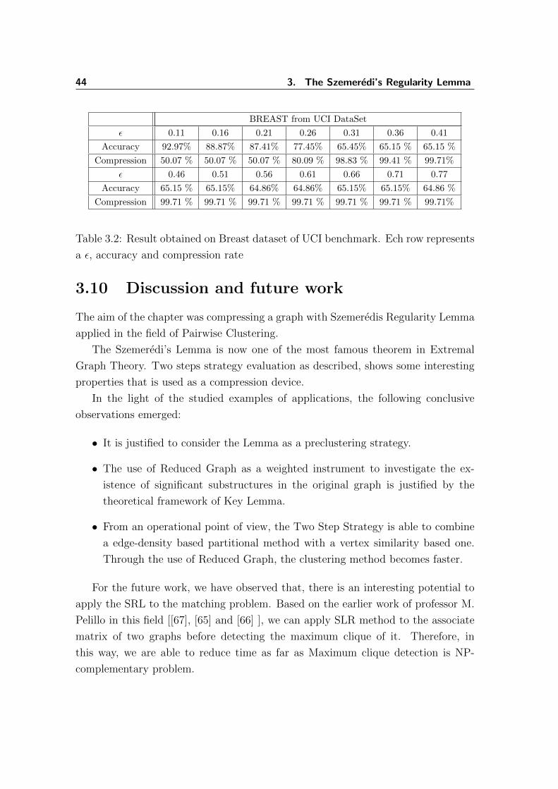
44 3. The Szemeredi’s Regularity Lemma
BREAST from UCI DataSet
ε 0.11 0.16 0.21 0.26 0.31 0.36 0.41
Accuracy 92.97% 88.87% 87.41% 77.45% 65.45% 65.15 % 65.15 %
Compression 50.07 % 50.07 % 50.07 % 80.09 % 98.83 % 99.41 % 99.71%
ε 0.46 0.51 0.56 0.61 0.66 0.71 0.77
Accuracy 65.15 % 65.15% 64.86% 64.86% 65.15% 65.15% 64.86 %
Compression 99.71 % 99.71 % 99.71 % 99.71 % 99.71 % 99.71 % 99.71%
Table 3.2: Result obtained on Breast dataset of UCI benchmark. Ech row represents
a ε, accuracy and compression rate
3.10 Discussion and future work
The aim of the chapter was compressing a graph with Szemeredis Regularity Lemma
applied in the field of Pairwise Clustering.
The Szemeredi’s Lemma is now one of the most famous theorem in Extremal
Graph Theory. Two steps strategy evaluation as described, shows some interesting
properties that is used as a compression device.
In the light of the studied examples of applications, the following conclusive
observations emerged:
• It is justified to consider the Lemma as a preclustering strategy.
• The use of Reduced Graph as a weighted instrument to investigate the ex-
istence of significant substructures in the original graph is justified by the
theoretical framework of Key Lemma.
• From an operational point of view, the Two Step Strategy is able to combine
a edge-density based partitional method with a vertex similarity based one.
Through the use of Reduced Graph, the clustering method becomes faster.
For the future work, we have observed that, there is an interesting potential to
apply the SRL to the matching problem. Based on the earlier work of professor M.
Pelillo in this field [[67], [65] and [66] ], we can apply SLR method to the associate
matrix of two graphs before detecting the maximum clique of it. Therefore, in
this way, we are able to reduce time as far as Maximum clique detection is NP-
complementary problem.

IVA Matrix Factorization Approach to
Graph Compression with Partial
Information

4A Matrix Factorization and Graph
Compression
He who has overcome his fears will
truly be free
Aristotle
4.1 Introduction
In the recent years, matrix factorization approaches have become an important tool
in machine learning and found successful applications for tasks like, e.g. information
retrieval, data mining and pattern recognition. Well-known techniques based on ma-
trix factorization are singular value decomposition, principal component analysis, la-
tent semantic analysis, non-negative matrix factorization and concept factorization.
Singular Value Decomposition (SVD) [38] decomposes without loss of information
any data matrix (not necessarily square) into the product of two unitary matrices
(left and right factors) and a non-negative diagonal matrix (central factor). Principal
Component Analysis (PCA) [41] is a statistical tool that determines an orthogonal
transformation to convert a set of observations of possibly correlated variables into
a set of values from linearly uncorrelated variables, known as principal components;
the principal components can actually be recovered through the SVD factorization.
Latent Semantic Analysis (LSA) [17] is another tool developed in the context of nat-
ural language processing that is based on the SVD factorization; this technique aims
at recovering hidden concepts from a typically sparse co-occurrence matrix of, e.g.
words and documents in the context of document analysis. Further developments of
LSA gave rise to the probabilistic Latent Semantic Analysis (pLSA) [36], which is

48 4. A Matrix Factorization and Graph Compression
based on a mixture decomposition of the latent class model, and to Latent Dirichlet
Allocation (LDA) [7], which is a more general generative model where observations
are explained by latent groups capturing the similarity structure within the data.
Non-negative Matrix Factorization (NMF) [47, 60] decomposes a non-negative data
matrix into the product of two non-negative factor matrices in a way to minimize the
divergence between the original matrix and the factorized one; several divergence
measures have been proposed including Frobenious distance, Kullback-Leibler di-
vergence, and more in general Bregman divergences. Some authors extended NMF
by integrating regularization terms acting on the factor matrices. Notably, in [11] a
method called Graph-regularized NMF (GNMF) is proposed, where the geometrical
manifold of the data points is used to regularize their low-dimensional representation
that is encoded in the non-negative right-factor matrix; a step forward is taken with
the Discriminative Orthogonal Non-negative (DON) matrix factorization approach
[49], which is characterized by an additional regularization term, aimed at rendering
the low-dimensional representations more discriminant. Furthermore, relations be-
tween NMF and clustering have been established in [20], where the authors show how
the k-means clustering formulation and the Laplacian-based spectral clustering for-
mulation can be cast into weighted, symmetrized instances of NMF. Similar works
shed light on a variety of further connections to graph matching, clique finding,
bi-clustering [21], pLSA [22] and hidden Markov models [46]. Some of those connec-
tions actually involve more complex, quadratic matrix factorization, i.e. exhibiting a
quadratic dependency on a factor matrix. Quadratic non-negative matrix factoriza-
tion methods under different types of constraints have recently been studied in more
details in [89, 90]. We end our brief introduction to matrix factorization techniques
with Concept Factorization (CF) [87], i.e. a matrix factorization method originally
introduced for document clustering that can be regarded as an auto-encoder model
for the data matrix, where the encoding and decoding steps are linear transforma-
tions. The resulting factorization is similar to NMF, but can also potentially deal
with non-negative data matrices. Recently, a regularized variant of CF has been
introduced [50], which takes into account the local, geometrical data structure in
kernel space.
A matrix undergoing a factorization in learning algorithms typically arises as
a collection of feature vectors, each vector being a column of the matrix, or as a
representation of the similarity/dissimilarity relations among data objects. In the
latter case, we can easily interpret the matrix as the adjacency matrix of a weighted
graph having the data objects as vertices. The application of matrix factorization

4.1. Introduction 49
for the analysis of graphs is mainly restricted to clustering [45, 72]. This paper aims
at giving a novel viewpoint about the role of matrix factorization in the analysis of
graphs and, in the specific, we show how matrix factorization can serve the purpose
of compressing a graph.
Compressing data consists in changing its representation in a way to require
fewer bits. Depending on the reversibility of this encoding process we might have a
lossy or lossless compression. Information-theoretic works on compressing graphical
structures have recently appeared [13]. However, they do not focus on preserving a
graph structure as the compressed representation, which is instead what we aim at
in our graph compression model. Our work is instead closer in spirit to [57], which
proposes a summarization algorithm for unweighted graphs, and [84], which proposes
a greedy procedure to determine a set of supernodes and superedges to approximate
a weighted graph. Moreover, our work is related to the Szemeredi regularity lemma
[80], a well-known result in extremal graph theory, which roughly states that a dense
graph can be approximated by a bounded number of random bipartite graphs. An
algorithmic version of this lemma has been used for speeding-up a pairwise clustering
algorithm in [78].
A problem linked to graph compression that has focused the attention of re-
searchers in the network and sociometric literature for the last few decades is block-
modeling [37, 51]. Block models try to group the graph vertices into groups that
preserve a structural equivalence, i.e. vertices falling in the same group should ex-
hibit similar relations to the nodes in other groups (including self-similarity), and
they differ by the way in which structural equivalence is defined. We refer to [29] for
an overview of blockmodels and to [2] for recent developments on mixed-membership
stochastic block models.
In this thesis we provide a novel viewpoint about the role of matrix factorization
in the analysis of graphs and, in the specific, for the purpose of compressing a graph.
The solution that we propose to compress a graph can be regarded as a block-model,
where blocks and their relationships can be determined using a matrix factorization
approach. Moreover, the model we propose extends our preliminary study in [59]
to deal with incomplete observation of the graph (or kernel) to be compressed. The
main contributions of the this chapter of thesis are the following:
i) we link matrix factorization with graph compression by proposing a factoriza-
tion that can be used to reduce the order of a graph and can be employed
also in the presence of incomplete observations. We show that the same tech-

50 4. A Matrix Factorization and Graph Compression
nique can be used to compress a kernel, by retaining a kernel as the reduced
representation;
ii) we cast the discrete problem of finding the best factorization into a continuous
optimization problem for which we formally prove the equivalence between the
discrete and continuous formulations;
iii) we provide a novel algorithm to approximately find the proposed factorization,
which resembles the NMF algorithm in [48] (under `2 divergence) and the Baum-
Eagon dynamics [5]. Additionally, we formally prove convergence properties for
our algorithm;
iv) finally, we establish a relation between clustering and our graph compression
model and show that existing clustering approaches in the literature can be
regarded as particular, constrained variants of our matrix factorization.
The rest of the manuscript is organized as follows. Section 4.2 introduces some
notation and basic definitions used in the work. Section 4.3 introduces our graph
compression formulation and its applicability also in the context of kernel compres-
sion. Section 4.4 addresses the problem of computing the factorization by proposing
an algorithm and by providing some convergence guarantees. Section 4.6 establishes
relations between the problem of clustering and our graph compression formula-
tion. Section 4.7 is devoted to showing the effectiveness of our graph compression
algorithm on both synthetic and real-world data-sets. Finally, we provide some
concluding discussion and plans for future developments.
4.2. Preliminaries 51
4.2 Preliminaries
We present here the notation and basic definitions adopted throughout the thesis.
General. We denote vectors with bold lowercase letters (e.g. x, y), matrices with
uppercase typewriter-style letters (e.g. A, B), sets with calligraphic-style uppercase
letters (e.g. X , Y). The (i, j)th element of matrix A is denoted by Aij, whereas the
ith element of a vector v is denoted by vi. We write indices with lowercase letters
(e.g. i, j, k, h) and constants with lowercase serif-style letters (e.g. n, m). We
denote by 1P the indicator function giving 1 if proposition P is true, 0 otherwise.
The sets of real and non-negative real numbers are given by R and R+ as usual. We
denote by [n] the set {1, . . . , n}.The pseudo-inverse x+ of a scalar x ∈ R returns 1/x if x 6= 0 and 0 otherwise.
The identity matrix is denoted by I. The vector of all 1s of size k is denoted by 1k,
the size being omitted where unambiguous. The matrix of all 1s is denoted by E.
Let A and B be two n × m matrix. The transposition of A is denoted as A>.
The inverse of a square matrix A is denoted by A−1. The set of left-stochastic
k × n matrices is given by S = {X ∈ Rk×n+ : X>1k = 1n} and we denote by
S01 = S∩{0, 1}k×n the set of left-stochastic binary matrices. Given A and B square,
the notation A < B means that (A−B) is positive semidefinite, i.e.
ij∈[n](Aij −Bij)xixj ≥ 0 for all x ∈ Rn
4.3 Matrix factorization for graph compression
An (edge-weighted) graph is a triplet (V , E , ω) where V = [n] is the set of n vertices,
E ⊆ V × V is the set of edges and ω : E → R is a function providing each edge
with a weight. We refer to n as the order of the graph. For the sake of simplicity,
we consider the graph to be complete and model missing edges as 0-weighted edges.
Moreover, the graph is assumed to be undirected and therefore ω(i, j) = ω(j, i)
for all (i, j) ∈ E . A graph (V , E , ω) can thus be encoded as a symmetric matrix
G ∈ Rn×n, where Gij = 1(i,j)∈Eω(i, j) or.
Gij =
ω(i, j) if (i, j) ∈ E
0 otherwise.
Hereafter, we might refer to G both as a graph or as a matrix depending on the
context.
52 4. A Matrix Factorization and Graph Compression
Let G ∈ Rn×n be a graph and let k ≤ n be a constant representing the order
of the new graph that we expect after the compression. The rate knis regarded as
the graph compression rate. To reduce the order of graph G from n vertices to k
vertices, we have to determine the compressed graph (or reduced graph) R ∈ Rk×k,
and a mapping ψ : [n] → [k] between vertices of the original graph G and the
reduced one R. The mapping ψ relates each vertex i of G to a vertex ψ(i) of R.
Since ψ is in general a many-to-one mapping, i.e. such that multiple vertices of G
can potentially be assigned to the same vertex of R, we have a lossless compression
only when the relation
Gij = Rψ(i)ψ(j) (4.1)
holds for all i, j ∈ [n]. In real-world scenarios, the graph might not be fully observed,
but only a subset of the entries in G might be available. To cope with this eventu-
ality, we assume that only a subset O ⊆ [n]× [n] of entries (not restricted to graph
edges) is observed. Due to the symmetry of G, we assume O to be symmetric as
well, i.e. (i, j) ∈ O =⇒ (j, i) ∈ O. If only partial information about the graph is
available, we relax the requirements for a “lossless” compression, by imposing that
(4.1) should hold just for all (i, j) ∈ O. From now on, we assume without loss of
generality that only partial information about the graph is available and that Oencodes the index set of the observed entries.
A many-to-one mapping ψ can be expressed as a left-stochastic binary matrix
X ∈ S01 where By expressing the many-to-one mapping ψ as a binary matrix X ∈{0, 1}k×n, having columns summing up to 1, i.e. X>1k = 1n, where each entry
Xkj = 1ψ(j)=k indicates whether vertex j of G should be assigned to vertex k of
R. On the other hand, every left-stochastic binary matrix X ∈ S01 encodes the
many-to-one mapping ψ(i) = arg maxkXkj. By replacing the mapping ψ with its
matrix-form counterpart X, we can compactly rewrite the condition for a lossless
compression (with partial observations O) in (4.1) in terms of the factorization
G=OX>RX . (4.2)
In general, a lossless factorization for a graph G at some fixed compression rate
might not exist. In this case, we resort to a least-squares approximation, i.e. we
look for a minimizer of
min g(X,R) = ‖G−X>RX‖2Os.t. X ∈ S01 , R ∈ Rk×k .
(4.3)

4.3. Matrix factorization for graph compression 53
The proposed factorization allows to reduce the complexity of the graph repre-
sentation from n2, i.e. the space complexity of G, to (n+k2), i.e. the effective space
complexity of (X,R). In fact, since matrix X is the matrix-form of the mapping ψ,
it can be stored more compactly as a n-dimensional vector, the ith component begin
index ψ(i). Additionally, it has interesting properties which render it suitable, e.g.
as a kernel compression strategy. Indeed, as a consequence of property 2 of Theorem
11, if G is a kernel and we have a complete set of observations (i.e. O = [n] × [n])
then also R is a kernel.
Theorem 11. Let (X,R) be a local solution of (4.3) with O = [n]× [n] and assume
X to have full rank. Then the following properties hold for any s ∈ {−1,+1}:
1. sG ∈ Rn×n+ =⇒ sR ∈ Rk×k
+ ,
2. sG < 0 =⇒ sR < 0.
Proof. By setting to zero the derivative of (4.3) with respect to R we obtain the
equationXGX> = XX>RXX> which must be satisfied by any local solution. Since
X ∈ S01 has rank k, matrix XX> is invertible. By left and right multiplying both
sides of the previous equation by (XX>)−1 we obtain (XX>)−1XGX>(XX>)−1 =
R. From this identity and assuming sG < 0 we can see that y>(sR)y = z>(sG)z ≥0 for all y ∈ Rk, where z = X>(XX>)−1y. Hence, Property 1 holds for anyX ∈ S01.Moreover also Property 2 holds, since (XX>)−1X is a non-negative matrix for any
X ∈ S01.
The assumption in Theorem 11 of X being of full rank is not restrictive. Indeed,
if X is rank deficient then it has at least one null row. By removing the null rows
of X and by dropping the corresponding rows and columns of R, we fall back to
the case where we have full rank without affecting the quality of the approximation.
Note also that property 1 holds, more in general, for any choice of O, while it is notnecessarily true for property 2.
54 4. A Matrix Factorization and Graph Compression
4.4 A tight relaxation of the graph compression
objective
The matrix factorization in (4.2) can be regarded as a particular quadratic factor-
ization, where the factor matrix X is left-stochastic and binary, and R is uncon-
strained. If we relax the binary constraint to a non-negativity constraint, we obtain
a quadratic matrix factorization that has been studied in [89] and for which update
rules have been indirectly provided.1 By using them, one could potentially find a
solution to (4.3) with S01 relaxed to S. However, by doing so, there is no guarantee
that the solution to the relaxed problem (once projected) will be also solution to
the original factorization problem, i.e. the relaxation is not tight. Moreover, the
update rules in [89] are not interior-point methods in the sense that feasibility is
not guaranteed at intermediate steps. In this section, we provide an alternative
relaxation to the graph compression objective, which is not per se in the form of a
matrix factorization problem, but it is tight as it allows to recover the solution to
(4.3). Moreover, the update rule we propose in Section 4.5 for Y is invariant to S,i.e. every iteration yields a feasible solution.
Instead of optimizing (4.3), which exhibits a non-convex feasible set, we optimize
a relaxation of the same program, where we drop the integer constraint. In the
specific, we replace the variable X ∈ S01 with a left-stochastic real matrix Y ∈S. This replacement is performed after some algebraic calculations which allow to
reduce the degree of the polynomial being the objective function. This yields the
following program:
min f(Y,R)
s.t. Y ∈ S , R ∈ Rk×k ,(4.4)
where
f(Y,R) =
(i,j)∈O
k,h∈[k]
1(k,i)6=(h,j)YkiYhj(Gij −Rkh)2 +
(i,i)∈O
k∈[k]
Yki(Gii −Rkk)2 .
The newly introduced optimization program satisfies a strong property provided
in Theorem 12, which suggests that (4.4) is a tight relaxation of (4.3) and that
minimizing (4.4) is equivalent to minimizing (4.3).
1there is no explicit update rule in the thesis to find the specific relaxed factorization, but it
could be obtained by using Theorem 1.
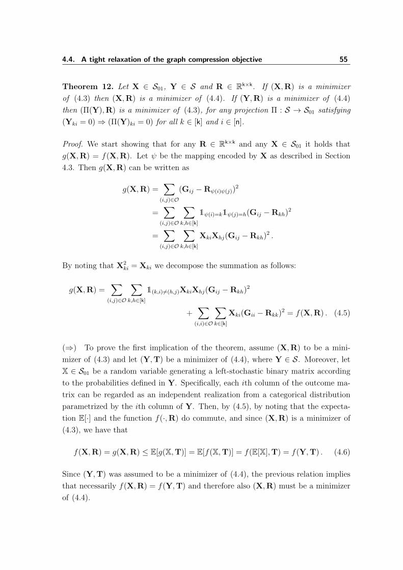
4.4. A tight relaxation of the graph compression objective 55
Theorem 12. Let X ∈ S01, Y ∈ S and R ∈ Rk×k. If (X,R) is a minimizer
of (4.3) then (X,R) is a minimizer of (4.4). If (Y,R) is a minimizer of (4.4)
then (Π(Y),R) is a minimizer of (4.3), for any projection Π : S → S01 satisfying
(Yki = 0)⇒ (Π(Y)ki = 0) for all k ∈ [k] and i ∈ [n].
Proof. We start showing that for any R ∈ Rk×k and any X ∈ S01 it holds that
g(X,R) = f(X,R). Let ψ be the mapping encoded by X as described in Section
4.3. Then g(X,R) can be written as
g(X,R) =
(i,j)∈O
(Gij −Rψ(i)ψ(j))2
=
(i,j)∈O
k,h∈[k]
1ψ(i)=k1ψ(j)=h(Gij −Rkh)2
=
(i,j)∈O
k,h∈[k]
XkiXhj(Gij −Rkh)2 .
By noting that X2ki = Xki we decompose the summation as follows:
g(X,R) =
(i,j)∈O
k,h∈[k]
1(k,i)6=(h,j)XkiXhj(Gij −Rkh)2
+
(i,i)∈O
k∈[k]
Xki(Gii −Rkk)2 = f(X,R) . (4.5)
(⇒) To prove the first implication of the theorem, assume (X,R) to be a mini-
mizer of (4.3) and let (Y,T) be a minimizer of (4.4), where Y ∈ S. Moreover, let
X ∈ S01 be a random variable generating a left-stochastic binary matrix according
to the probabilities defined in Y. Specifically, each ith column of the outcome ma-
trix can be regarded as an independent realization from a categorical distribution
parametrized by the ith column of Y. Then, by (4.5), by noting that the expecta-
tion E[·] and the function f(·,R) do commute, and since (X,R) is a minimizer of
(4.3), we have that
f(X,R) = g(X,R) ≤ E[g(X,T)] = E[f(X,T)] = f(E[X],T) = f(Y,T) . (4.6)
Since (Y,T) was assumed to be a minimizer of (4.4), the previous relation implies
that necessarily f(X,R) = f(Y,T) and therefore also (X,R) must be a minimizer
of (4.4).

56 4. A Matrix Factorization and Graph Compression
(⇐) To prove the other implication of the theorem, assume (Y,R) to be a min-
imizer of (4.4) and let (X,T) be a minimizer of (4.3). Then, similarly to (4.6),
we have that f(Y,R) = E[g(X,R)] ≥ g(X,T) = f(X,T). This implies that
E[g(X,R)] = g(X,T) since (Y,R) is assumed to be a minimizer of (4.4) and there-
fore g(Z,R) = g(X,T) for all Z ∈ S01 such that P[X = Z] > 0. Now, since
P[X = Π(Y)] > 0 by construction, it follows that (Π(Y),R) is a minimizer of
(4.3).
According to Theorem 12, we can focus on the optimization of (4.4), which has a
continuous objective and domain, in place of (4.3), for any solution Y∗ of the former
can be cast into a solution X∗ of the latter by applying a projection as defined by
the theorem, i.e. X∗ = Π(Y∗). As an example of such a projection, we could replace
each column of Y∗ with an indicator vector for the largest element in the column to
obtain X∗.

4.5. Graph compression algorithm 57
4.5 Graph compression algorithm
We propose an optimization approach for (4.4), which alternates updates of the
variable R and updates of the variable Y. Both updates are shown to deliver a
decrease of the objective function until a stationary point of (4.4) is reached.
4.5.1 Update rule for R.
Since R is an unconstrained matrix variable, we derive an update rule for it by
setting the first-order partial derivative of f with respect to its second argument R
to zero (see, proof of Theorem 13 for details). This yields
UR(Y)kh = (Lhk)+
(i,j)∈O
1(k,i) 6=(h,j)YkiYhjGij + 1k=h
(i,i)∈O
YkiGii
, (4.7)
where L is defined as
Lkh =
(i,j)∈O
1(k,i)6=(h,j)YkiYhj + 1k=h
(i,i)∈O
Yki . (4.8)
This update rule has complexity O(k2|O|) and guarantees a monotonic decrease of
the objective function f as stated by the following theorem.
Theorem 13. Let T ∈ Rk×k and Y ∈ S. Then
f (Y,T) ≥ fY, UR(Y)
with equality if and only if T is a minimizer of f(Y, ·).
Proof. Since f(Y, ·) is a quadratic form and it is lower bounded by 0, we can prove
the result by simply showing that
∂f
∂Rkh
(Y, UR(Y)) = 0 . (4.9)
Indeed, if this is true, then UR(Y) will be a global minimizer of f(Y, ·) and therefore
f(Y,T) = f(Y, UR(Y)) holds true if and only if T is a global minimizer of f(Y, ·)as well.

58 4. A Matrix Factorization and Graph Compression
The partial derivative of f with respect to its second argument R is given by
∂f
∂Rkh
(Y,R) = 2
(i,j)∈O
1(k,i)6=(h,j)YkiYhj(Rkh −Gij)
+ 2
(i,i)∈O
1k=hk∈[k]
Yki(Rkh −Gii)
= 2RkhLkh − 2
(i,j)∈O
1(k,i) 6=(h,j)YkiYhjGij
− 2
(i,i)∈O
1k=hk∈[k]
YkiGii ,
where L is defined as in (4.8). By expanding the derivative in (4.9), by isolating
the term with UR(Y)on the left-hand-side of the equation, and after halving both
sides, we get
[UR(Y)]khLkh =
(i,j)∈O
1(k,i) 6=(h,j)YkiYhjGij + 1k=h
(i,i)∈O
YkiGii . (4.10)
Clearly, by definition of UR(Y), the equality holds true if Lkh 6= 0. In the other
case, Lkh = 0 only if YkiYhj = 0 for all (i, j) ∈ O. This in turn implies that
the right-hand-side of (4.8) is zero as well. Hence, if Lkh = 0 then (4.10) is always
satisfied and in particular it is satisfied by the update rule (4.7), which would deliver
UR(Y)kh = 0, for (Lkh)+ = 0+ = 0.
4.5.2 Update rule for Y.
We derive here a multiplicative update rule for Y, which resembles the one proposed
in [48] for Non-negative Matrix Factorization (NMF) under `2 divergence and the
one related to the Baum-Eagon inequality [5].
Let R ∈ Rk×k and Z ∈ S and consider the following optimization problem:
min fR(Y) = f(Y,R)
s.t. Y ∈ YZ(4.11)
where YZ = {Y ∈ S : (Zki = 0)⇒ (Yki = 0)}. We say that Y is a Karush-Kuhn-
Tucker (KKT-)point for (4.11) if it satisfies the first-order necessary conditions for

4.5. Graph compression algorithm 59
local optimality, which are given by:
∂fR∂Yki
(Y)− γi − µki − αki1Zki=0= 0 , (4.12)
µkiYki = 0 , (4.13)h∈[k]
Yhi = 1 , (4.14)
Yhi1Zki=0= 0 , (4.15)
for some values of the Lagrangian multipliers γi, αki ∈ R and µki ∈ R+, for all k ∈ [k]
and i ∈ [n].
Let σi(Z) be the support of the ith column of Z, i.e. σi(Z) = {k ∈ [k] : Zki > 0},and let Zi(Z,R), i ∈ [n], denote the set
Zi(Z,R) =
k ∈ [k] :
∂fR∂Yki
(Z) = 0
∩ σi(Z) .
The following update rule UY(Z,R) for Y guarantees a strict decrease of the
objective function in (4.11) unless Z is a KKT-point (see Theorem 14):
UY(Z,R)ki =
0 if k /∈ σiZki
h∈Zi
Zhiif k ∈ Zi
Zki
λi∂fR∂Yki
(Z)
if Zi = ∅, k ∈ σi
(4.16)
where we wrote σi and Zi for σi(Z) and Zi(Z,R), and where
λi =h∈σi
Zhi∂fR∂Yhi
(Z)−1 .
The complexity of this update rule is O(k2|O|) (see (4.19) for the formula of the
first-order partial derivative).
Theorem 14. Let R ∈ Rk×k and Z ∈ S. Then
f(Z,R) ≥ f(UY(Z,R),R)
with equality if and only if Z is a KKT-point for (4.11).

60 4. A Matrix Factorization and Graph Compression
Before providing the proof of Theorem 14, we need the following lemma:
Lemma 6. Let Z ∈ S and consider the following function:
φ(Y,Z) = fR(Z) +i∈[n]
k∈[k]
(Yki − Zki)∂fR∂Yki
(Z)
+1
2
i∈[n]
k∈[k]
(Yki − Zki)2 ∂fR∂Yki
(Z)Z+ki . (4.17)
Then φ(Y,Z) ≥ fR(Y) for all Y ∈ YZ.
Proof. By replacing fR with its Taylor expansion about Z we obtain after simple
algebraic manipulations:
φ(Y,Z)− fR(Y) =1
2
i∈[n]
k∈[k]
(Yki − Zki)2 ∂fR∂Yki
(Z)Z+ki
− 1
2
i,j∈[n]
k,h∈[k]
(Yki − Zki)(Yhj − Zhj)∂2fR
∂Yki∂Yhj
(Z) , (4.18)
where the first-order and second-order partial derivatives are given by
∂fR∂Yki
(Z) = 1(i,i)∈O(Gii −Rkk)2 +
j∈[n]
h∈[k]
1(i,j)∈O1(k,i)6=(h,j)Zhj (Gij −Rkh)2
≥j∈[n]
h∈[k]
1(i,j)∈O1(k,i)6=(h,j)Zhj (Gij −Rkh)2 , (4.19)
and∂2fR
∂Yki∂Yhj
(Z) = 1(i,j)∈O1(k,i)6=(h,j)(Gij −Rkh)2 , (4.20)
respectively.
Let Qki = (Yki − Zki)Z+ki and note that QkiZki = (Yki − Zki) for all Y ∈ YZ,
because Zki = 0 implies Yki = 0 by definition and ZkiZ+ki = 1Zki>0
. Accordingly,
we can rewrite (4.18) as
φ(Y,Z)− fR(Y) =1
2
i∈[n]
k∈[k]
Q2kiZki
∂fR∂Yki
(Z)
− 1
2
i,j∈[n]
k,h∈[k]
QkiQhjZkiZhj∂2fR
∂Yki∂Yhj
(Z) ,

4.5. Graph compression algorithm 61
By substitution of (4.19) and (4.20) and by reorganizing the terms we obtain the
following inequality
φ(Y,Z)− fR(Y) ≥ 1
2
(i,j)∈O
k,h∈[k]
ZkiZhj1(k,i)6=(h,j)(Gij −Rhk)2Q2ki −QkiQhj
.
By exploiting the symmetry of G and R, we have
φ(Y,Z)− fR(Y) ≥
(i,j)∈O
k,h∈[k]
ZkiZhj1(k,i)6=(h,j)
· (Gij −Rhk)2
1
2Q2ki −QkiQhj +
1
2Q2hj
≥ 0 . (4.21)
where the last inequality follows from (12Q2ki−QkiQhj +
12Q2hj) =
12(Qki−Qhj)
2 ≥ 0
and the non-negative of all other terms.
Proof of Theorem 14. LetY∗ = UR(Z,R). We start proving thatY∗ is a minimizer
of
minY∈YZ
φ(Y,Z) , (4.22)
where φ is defined as in (4.17).
A minimizer Y of (4.22) must be a KKT-point for it. The conditions that should
be satisfied are (4.13), (4.14), (4.15) and
∂φ
∂Yki
(Y,Z)− γi − µki − αki1Zki=0= 0 (4.23)
for all k ∈ [k] and i ∈ [n], where γi, αki ∈ R and µki ∈ R+ are the Lagrangian
multipliers. It is immediate to see that (4.14) and (4.15) are always satisfied by Y∗.
If Zki = 0 then (4.23) is trivially satisfied as αki can take any value, and, since by
definition of Y∗, Zki = 0 implies Y∗ki = 0, also (4.13) is satisfied. On the other hand,
if Zki > 0 we have by definition of Y∗ that Y∗ki > 0 and by taking µki = 0, we have
that (4.13) is satisfied. Now, if Zi = ∅ then it is easy to verify, after substituting Y∗
with its definition, that (4.23) is satisfied by setting γi = λ−1i , while if Zi 6= ∅ then
(4.23) is satisfied by taking γi = 0. This proves that Y∗ is a KKT-point for (4.22).
Since (4.22) is a convex optimization problem, we have that any KKT-point is also
a global minimizer and therefore Y∗ is a minimizer of (4.22).
By this result and by Lemma 6 we have that
f(Z,R) = fR(Z) = φ(Z,Z) ≥ φ(Y∗,Z) ≥ fR(Y∗) = f(UR(Z,R),R) . (4.24)

62 4. A Matrix Factorization and Graph Compression
To conclude the proof, assume Z to be a KKT- point of (4.11). Trivially Y∗ki =
Zki by definition of Y∗, if Zki = 0. Assume now Zki > 0. Then by (4.12) we have
that∂fR∂Yki
(Y) = γi. By exploring this fact in the definition of Y∗ we can easily
derive that also in this case Y∗ki = Zki. Hence, Y∗ = Z and therefore (4.22) holds
with equality. On the other hand, assume that (4.24) holds with equality. Then
fR(Z) = φ(Y∗,Z). This implies that Z is a solution of (4.22) and a KKT-point
for it. Hence, Z satisfies the conditions (4.23), (4.13), (4.14) and (4.15). Now, since∂φ
Yki(Z,Z) =
∂fR∂Yki
(Z), it follows that Z satisfies also (4.12) and therefore it is a
KKT-point also for (4.11).
4.5.3 Summary of the algorithm.
The proposed optimization procedure summarized in Algorithm 4.1 works as follows.
We start with a random matrix Y lying in the interior of S. We repeatedly alternate
between updating R as R ← UR(Y) and Y as Y ← UY(Y,R). We iterate
until some stopping criterion is met, e.g. distance between Ys of two consecutive
iterations is below a given threshold, maximum number of iterations reached, etc.
According to Theorem 13 and 14, this procedure guarantees a strict decrease of the
objective in (4.3) until a KKT-point is reached. This might not correspond to a
local minima, but e.g. a saddle point. By inducing a small local perturbation and
by restarting the procedure we can escape from a saddle point with high probability.
In this way, we can ensure that a local solution will be reached. Finally, we project
Y on S01 by means of a projection operator Π satisfying the properties stated in
Theorem 12. As an example of Π, we can set to 1 in each column of Y the element
having highest value (in the column) and put to 0 the rest. The complexity of the
algorithm is O(|O|k2β) if we have partial information and O(n2kβ) if we employ
the full graph G. Here, β denotes the expected number of iterations required to
converge.
4.5.4 Graph reconstruction with incomplete observations
In Section 4.3 we envisaged the possibility of having only partial information about
the graph, which translates into a restricted set O of observed edges. As we have
shown, our graph compression algorithm can cope with this eventuality and yet
deliver the reduced graph R and the corresponding mapping X, begin solution of
(4.3). The advantage of this feature is that we can provide a reconstructed version
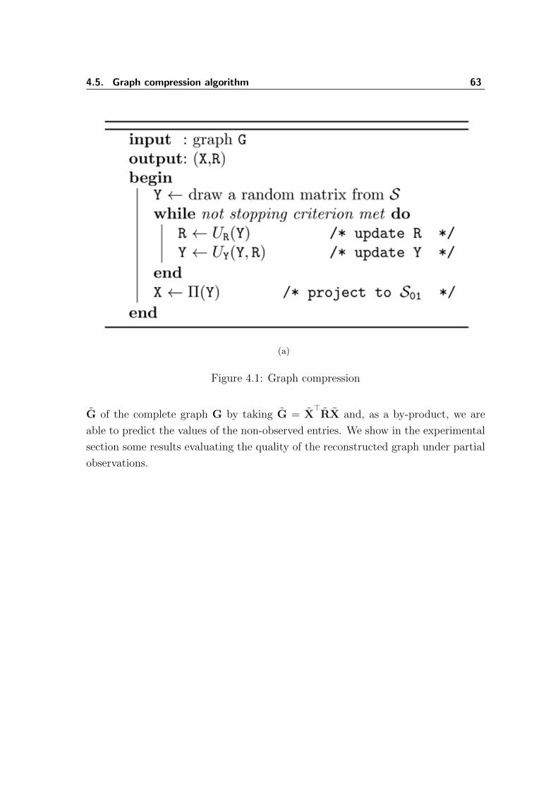
4.5. Graph compression algorithm 63
(a)
Figure 4.1: Graph compression
G of the complete graph G by taking G = X>RX and, as a by-product, we are
able to predict the values of the non-observed entries. We show in the experimental
section some results evaluating the quality of the reconstructed graph under partial
observations.

64 4. A Matrix Factorization and Graph Compression
4.6 Clustering as graph compression
Although clustering is not the main focus of this thesis, it is interesting to point
out the relation that exists between our graph compression and clustering (see, [29]
for a more comprehensive discussion specific to block-models). Under our model,
clustering can be regarded as a graph compression if we interpret the vertices of the
reduced graph as the clusters. From this perspective, the mapping X encodes the
clustering result. Now, if we consider a cluster as Before coming to the experiment,
it is worth mentioning that the notion of cluster under this setting differs from the
commonly accepted one of a set of elements being mutually similar and dissimilar
to elements belonging to other clusters, which is the commonly accepted definition,
then the related compression should exhibit a reduced graph being loosely connected
with strong weight on the self-loops, In other words, we expect R ≈ I.
Interestingly, we found out that some clustering algorithms proposed in the liter-
ature can be regarded as constrained variants of our graph compression method. In
[71] a consensus clustering approach has been proposed based on the optimization of
a functional like (4.3) with the integer constraint dropped and under the condition
R = I. A clustering model similar to this one has been proposed also for community
detection in [58]. Finally, in [72] a pairwise clustering approach with probabilistic
cluster assignments has been proposed, which enforces the milder condition R = αI,
α being a nonnegative variable to optimize.
In general, an optimal graph compression under our model does not necessarily
conform to a clustering outcome. As an intuitive example of this fact, consider
a complete bipartite graph (V , E), where V = A ∪ B and E = A × B. In this
case, a lossless compression can be obtained by taking k = 2, R = E − I and
Xki = 1k=11i∈A+1k=21i∈B. If we try to interpret this as a clustering result, our two
clusters are A and B. These two sets, however, are both internally highly dissimilar
and externally very similar, yielding a contradistinction with the standard definition
of cluster. This suggests that Still, clustering results being conformal to the standard
notion can be extracted, e.g. in case of block-structured nearly diagonal matrices,
but the type of analysis that can be potentially conducted with our method has a
spectrum that is broader than clustering.

4.7. Experiments 65
4.7 Experiments
We conducted both synthetic and real-world experiments to assess the effective-
ness of the proposed graph compression method. Additionally, we performed some
experiments on clustering motivated by the discussion conducted in Section 4.6.
4.7.1 Synthetic experiments
For the first experiment, we created a data-set of weighted graphs that can be in
principle compressed without loss of information. Each instance having order n =
400 was generated by randomly sampling the matrix X ∈ S01, the compressed graph
R ∈ [0, 1]k×k and by computing G as X>RX. We considered compression rates
varying between 2−7 and 2−2. For each level of compression, we randomly generated
40 graph instances. We evaluated the solution found (X, R) by our algorithm in
terms of the average entry-wise matrix reconstruction error, i.e. ‖G−X>RX‖F/n2.
In Figure 4.2(a), we report for each level of compression (in log2-scale) the error,
averaged over the 40 graph instances, and the corresponding standard deviation.
The overall performance of the algorithm is good as we achieve a low entry-wise
error in the reconstruction. Nevertheless, we do not always achieve the lossless
compression due to the existence of local solutions, begin close to the optimal one.
We also notice that the reconstruction error is lower at higher levels of compression.
In Figure 4.3, we report the evolution of the objective f(Y,R) of 6 executions
of our algorithm. Each execution is performed on a random graph of order n = 400
generated as described in the previous paragraph that can be compressed with the
value of k adopted for the specific run. The different values of k reported in the
legend correspond to compression rates ranging from 2−7 to 2−2. We notice that
the objective is monotonically decreasing as stated by our theorems and that the
objective stabilizes in a number of steps that grows with the value of k.2 All runs
are characterized by an initial slow decay of the objective followed by a drastic
decrease, which culminates in a stable limit. In our experience, depending on the
initial random guess of Y, this transition between slow and fast descent might
eventually occur more than one time.
In a second experiment, reported in Figure 4.2(b), we generated graphs that
2this however should not be taken as a truth holding in general, for it depends also on the
structure of the input graph.

66 4. A Matrix Factorization and Graph Compression
are factorizable (as previously detailed) but at a fixed compression rate k/n = 0.1.
We corrupted the factorizable graphs with different levels of Gaussian noise. By
doing so, the existence of a lossless compression is not guaranteed anymore. We
considered 40 graph instances per noise level and we reported the average entry-
wise reconstruction error (with respect to the noise-less graph) and the standard
deviation obtained with our algorithm when trying to compress the noisy graph. To
have a clue of the incidence of noise, we report the reconstruction error of the ground-
truth factorization with respect to the noisy graph G, i.e. ‖X>RX− G‖F/n2. As
we can see, at low noise levels our algorithm provides a compression yielding a good
reconstruction, even though it is not the optimal one due to the existence of local
solutions. The robustness of our algorithm becomes however clear at higher levels of
noise, where our reconstruction error remains significantly below the error induced
by the corruption, which means that we achieve a good signal-to-noise ratio.
In a third experiment, we deal with unweighted graphs and structural noise.
We created a dataset of graphs, each having order 400 and being generated in the
following way. We sampled the matrix X ∈ S01 and we sampled a random matrix
R ∈ [0, 1]k×n with 50% of its components set to 0. We computed then G = X>RX
and considered each entry of the resulting matrix as the probability of observing
an edge. Finally, we created the graph instance by sampling each edge according
to the corresponding probability. By reiterating this procedure, we generated 40
graphs for each compression rate ranging between 2−7 and 2−2. We try to pursue
the ambitious goal of recovering the vertex partition induced by X by means of our
graph compression algorithm. If (X, R) are the factorization parameter recovered
by our algorithm, we evaluated the quality of the reconstruction by comparing the
partitions induced by X and X in terms of classification accuracy. In Figure 4.2(c),
we report the average accuracy with standard deviation that we obtained at varying
levels of compression (in log2-scale). We achieved impressively high accuracies at all
the compression levels that we considered. This success reveals that the proposed
factorization allows to recover information about the random process adopted to
generate the graphs and confirms the existence of strong links with the Szemeredi
regularity lemma as mentioned in the introduction.
Finally, we performed a last synthetic experiment, which takes into account par-
tial information. We generated 3 sets of 10 graph, each graph having 500 nodes.
The first set consists of Erdos-Renyi-type random graphs with density 0.01, which
lack any structure. The second and third set are synthetic unstructured and struc-
tured community graphs generated according to the following procedure reflecting

4.7. Experiments 67
the generative model described in [54]. Each node is assigned to a cluster accord-
ing to a Chinese restaurant process, where the probability of being assigned to an
existing cluster is proportional to the size of the cluster, with a non-zero proba-
bility proportional to α of being assigned to a new cluster. In our experiments
we set α = 5 for either type of community graphs. Once the clusters have been
determined, undirected edges between vertices are sampled independently accord-
ing to a probability that depends on their cluster assignments. Within-custer link
probability η`` of cluster ` is sampled from a Beta distribution with parameters
(ain, bin), while the between-cluster link probability between clusters ` and m is
sampled according to a Beta distribution with parameters (aout, bout). In the case
of structured community graphs, the Beta distribution for the between-cluster links
is constrained to the interval [0, x`m], where x`m = min{γ`η``, γmηmm} and γ` de-
notes the cluster gap probability of cluster ` being sampled from a Beta distribution
with parameters (agap, bgap). The parametrization used to generate the unstruc-
tured community graphs is aout = bout = ain = 1 and bin = 10, while the one
used to generate the structured community graphs is aout = ain = agap = 1 and
aout = bout = bgap = 10. Intuitively, the structured community graphs are created in
a way to fulfill the property that communities have more internal than external links,
as opposed to unstructured community graphs. We compare our algorithm against
other approaches, which are specifically tuned for this graph generation model as
opposed to our approach: Infinite Relational Model (IRM), Infinite Diagonal Model
(IDM) and Bayesian Community Detection (BCD). We used the implementation of
these approaches provided by the authors of BCD [54]. In Table 4.1 we report the
ability of each approach to predict the missing edges in terms of average Area-Under-
Curve (AUC). The results show that with a random setting the prediction of each
algorithm is worthless, yielding AUC≈0.5. Indeed, those graphs lack a regularity,
which renders the link-state discrimination difficult to achieve. As the information
becomes more structured, our approach yields competitive results (AUC>80%). In
fact, both structured and unstructured community graphs present a marked block-
wise arrangement. These graphs can be effectively compressed and good levels of
state-link discrimination can thus be achieved. The structured community graphs
are slightly more regular than the unstructured ones, due to the constrained number
of between-cluster versus within-cluster links, which motivates the improved AUC
value (+3%).

68 4. A Matrix Factorization and Graph Compression
Methods
DataSet IRM IDM BCD Graph Compression
Random 0.50 ± 0.01 0.50 ± 0.02 0.50 ± 0.02 0.50 ± 0.02
Unstructured 0.83 ± 0.01 0.45 ± 0.01 0.78 ± 0.01 0.81 ± 0.01
Structured 0.77 ± 0.03 0.67 ± 0.01 0.83 ± 0.01 0.84 ± 0.01
Table 4.1: Experimental results on Erdos-Renyi random graphs for the task of
predicting the state of non-observed edges. We consider three different scenarios:
purely random graph, unstructured graph and structured graph. We report the
average AUC value (and standard deviation) obtained with 10 graph samples per
setting.
4.7.2 Real-world experiments
In real-world scenarios, the graphs to be compressed do not exhibit necessarily a
lossless compression at a given compression rate. Therefore, as opposed to the syn-
thetic case, we try to determine the quality of the factorization in a more pragmatic
way. We analyses the performances of some algorithms working on graphs and ker-
nels, when applied to the original matrix G and to the reconstructed matrix X>RX
at different compression rates, (X, R) being the solution found by our algorithm.
The rationale of this experiment is that a good compression, having a low loss,
will not impact the performance of an algorithm significantly, if we run it on the
reconstructed graph/kernel rather than the original one.
We performed a first set of experiments on clustering with a spectral algorithm
(SC) working on graphs [76] and with the Kernel K-Means algorithm (KKM) work-
ing with a kernel [18]. Table 4.2 reports the classification accuracies obtained by the
two algorithms on different machine learning data-sets, namely Iris, Wine, Haber-
man, Pima, BloodT and Imox. Each algorithm was run on a graph/kernel recon-
structed after having been compressed with a rate varying between 2−5 and 1 (in the
tables we reported the rate in log2-scale). The results obtained at rate 1 represent
the performance of the algorithms on the original data, without compression. As we
can see, the accuracies reported are not significantly affected due to the compression,
even at low rates. In some cases, we notice an increase of the performance at some
intermediate compression levels (see, e.g. Imox for KKM and Haberman for SC).
We performed also some qualitative experiments on dimensionality reduction
with Kernel- Principal Component Analysis (KPCA) [75]. We report in Figure 4.4

4.7. Experiments 69
(a) Kernel K-Means
Compression rate
Dataset n k 1/32 1/16 1/8 1/4 1/2 1
Iris 150 3 0.85 0.85 0.89 0.90 0.91 0.91
Wine 178 3 0.56 0.72 0.72 0.72 0.71 0.73
Haberman 306 2 0.65 0.65 0.65 0.65 0.65 0.65
Pima 768 2 0.78 0.89 0.81 0.89 0.89 0.90
BloodT 748 2 0.41 0.40 0.38 0.39 0.40 0.39
Imox 192 4 0.75 0.88 0.86 0.87 0.77 0.78
(b) Spectral Clustering (Normalized Cut)
Compression rate
Dataset n k 1/32 1/16 1/8 1/4 1/2 1
Iris 150 3 0.85 0.85 0.89 0.90 0.89 0.89
Wine 178 3 0.71 0.57 0.71 0.59 0.57 0.58
Haberman 306 2 0.50 0.73 0.73 0.71 0.71 0.64
Pima 768 2 0.78 0.89 0.87 0.89 0.89 0.91
BloodT 748 2 0.41 0.42 0.40 0.40 0.40 0.41
Imox 192 4 0.75 0.78 0.78 0.77 0.79 0.79
Table 4.2: Clustering results obtained by Kernel K-means and Spectral Cluster-
ing (Normalized Cut) on different data-sets, after having compressed the data
(graph/kernel) at different rates.
the data points of two machine learning data-sets, namely Iris and eColi, repro-
jected on the 3 principal components found with K-PCA and colored according to
the ground-truth classes. For each data-set, we performed the analysis using both
the original kernel (compression rate 1) and the same kernel reconstructed after
having been compressed with rate 0.0625. As we can see, the degree of separation
of the classes between the analysis conducted on the original kernel and on the
reconstructed one are comparably good.
Finally, we perform a set of experiments to test the effectiveness of our ap-
proach under partial information on several real-world data-sets: Friend, Ecoli,
Yeast, MIPS, Friend Same Sex, Friend Same Race, Caltech, Macaque and Lesmis.
For each dataset we consider 10 random splits consisting of 80% of the input ma-
trix G for training and 20% for testing. The training entries of the input matrix
are used to compute the factorization, while the test entries are used to assess the
quality of the predictions obtained using the computed factorization. We compare
against Non-Negative Matrix Factorization (NMF) [48], which is a well-known ma-

70 4. A Matrix Factorization and Graph Compression
trix factorization approach that factorizes an interaction matrix to low-dimensional
representations with non-negativity constraints and has also been employed for com-
munity detection (see, e.g. [69]), and against Graph-regularized NMF (GNMF) [11],
which is a recent, regularized variant of NMF. In Table 4.3 we report the results ob-
tained in terms of AUC under different values of k.3 When we have high compression
rates (k = 3) NMF and GNMF yield better results on most of the data-sets. This is
not surprising because the number of parameters to optimize with k = 3 is larger in
NMF/GNMF than our approach and can thus better capture the matrix structure
than we do. However, this over-parametrization has a negative effect as we increase
k from 3 to 5 and 7, for our approach achieves the best results on 5/9 and 6/9 data-
sets, respectively. Also this experiment shows that our model can better compress
the information encoded in the structural data without loosing the most significant
signals. Finally, we think that it is due remarking that, as opposed to NMF and our
approach, GNMF comprises a free parameter than has to be tuned, which balances
the matrix approximation term and the regularization term. We have manually
tuned it to deliver better results, but wrong choices of this parameter might lead to
bad results. Nevertheless, our approach turned out to be competitive despite this
handicap.
3for NMF and GNMF this coincides with the number of latent dimensions

4.7. Experiments 71
NMF GNMF Graph Compression
DataSet n 3 5 7 3 5 7 3 5 7
Friend 900.78 0.72 0.75 0.84 0.79 0.79 0.78 0.80 0.79
(0.00) (0.02) (0.01) (0.01) (0.00) (0.00) (0.01) (0.01) (0.01)
Ecoli 2300.82 0.82 0.82 0.80 0.82 0.82 0.75 0.84 0.88
(0.01) (0.01) (0.00) (0.00) (0.00) (0.01) (0.00) (0.02) (0.01)
Yeast 2830.84 0.88 0.84 0.86 0.89 0.89 0.74 0.80 0.83
(0.01) (0.01) (0.00) (0.01) (0.01) (0.00) (0.00) (0.00) (0.00)
MIPS 8710.81 0.85 0.87 0.91 0.93 0.94 0.91 0.94 0.97
(0.01) (0.00) (0.00) (0.00) (0.00) (0.00) (0.00) (0.00) (0.00)
Fr S. S. 900.97 0.98 0.99 1.00 1.00 1.00 0.99 0.99 1.00
(0.00) (0.00) (0.00) (0.00) (0.00) (0.00) (0.00) (0.00) (0.00)
Fr S. R. 900.92 0.96 0.99 0.96 0.96 0.96 0.99 0.99 1.00
(0.00) (0.00) (0.00) (0.00) (0.00) (0.00) (0.00) (0.00) (0.00)
Calthec 7620.87 0.90 0.91 0.88 0.90 0.91 0.78 0.80 0.81
(0.00) (0.00) (0.00) (0.00) (0.00) (0.00) (0.00) (0.00) (0.00)
Macaque 470.86 0.81 0.81 0.89 0.87 0.85 0.77 0.81 0.83
(0.01) (0.02) (0.01) (0.01) (0.01) (0.01) (0.02) (0.01) (0.00)
Lesmis 770.88 0.84 0.83 0.86 0.86 0.81 0.86 0.90 0.89
(0.00) (0.01) (0.01) (0.01) (0.01) (0.02) (0.00) (0.01) (0.02)
Table 4.3: Experimental results on real-world data-sets for the task of predicting the
state of non-observed edges. We report the average AUC (and standard deviation)
obtained with 10 random training/test set (80%/20%) splits.
4.7.3 Clustering
Motivated by the relation that exists between graph compression and clustering, as
pointed out in Section 4.6, we tried to interpret the outcome of our graph compres-
sion algorithm as it were a clustering result. We performed experiments on syn-
thetic and real-world machine learning data-sets, namely the S100 Block Stochastic
(S-Block) dataset [86], the Iris dataset (Iris), the NIST handwritten digits dataset
(Digit), a subset of the SCOP protein dataset (Scop) [39] and the Wine dataset. We
performed a graph compression with k tuned to the optimal number of clusters for
each dataset and we considered the factorization parameter X found by our graph
compression algorithm as the clustering result. To escape local minima we run our
algorithm 10 times and kept the solution exhibiting lowest reconstruction error. We
report as evaluation measure the classification accuracy for each dataset of our so-
lution against the ground truth solution. Due to the relation shown in Section 4.6

72 4. A Matrix Factorization and Graph Compression
between our graph compression method and the Baum-Eagon (BE) clustering algo-
rithm [72], we report for the sake of comparison the scores from the original paper
for the data-sets where BE has been applied. As we can see from Figure 4.5, in all
data-sets, excepting Digit the compression delivered by our method correlates well
with the data-set’s ground truth. Compared to BE, we perform slightly worse on
Iris, S-Block and perform very bad on Digit. This is however an expected scenario.
Indeed, according to the discussion done in Section 4.6, a good graph compression
might not conform to a standard clustering result. The results obtained on Digit
support this fact as we verified that the factorization found on digit, despite being
very far from the ground-truth clustering, delivered a low reconstruction error, thus
providing a good compression. The comparison with BE also reveals that by adding
a constraint in our model enforcing the compression to fulfill the properties of a
clustering, the results can clearly improve, one exception being Scope. We conclude
remarking that the goal of this section is not to show that our method can be used
as a clustering algorithm, but we considered interesting to emphasis the relation
between clustering and graph compression also from an experimental perspective.

4.8. Discussion and future work 73
4.8 Discussion and future work
In this chapter, we have proposed a novel matrix factorization, which can be used
to compress graphs and kernels, also in the presence of missing observations about
the edges of the graph to be compressed. We have introduced an algorithm for
finding such a factorization in an approximate way. Interestingly, we came up with
an update rule which resembles the ones adopted for NMF and the one introduced
by Baum and Eagon for maximizing polynomials with non-negative coefficients in
probability domain. We have proven convergence properties of these update rules
and we think that similar optimization dynamics can be employed for other types
of matrix factorization in probability domain.
Besides data analysis, our graph compression can be potentially employed to
speed-up existing graph-based and kernel-based algorithms. We did not address
this topic in this chapter since our focus was to show the effectiveness of our graph
compression formulation. However, the experiments conducted in Section 4.7.2 ev-
idenced that the information preserved by the compression is sufficient to avoid
drastic decay of the algorithm’s performances. Actually, we experienced a constant
performance even at low compression rates. The complexity of many algorithms
can be reduced by replacing G with the factorization X>RX and by exploiting the
sparsity of X. As an example, the complexity of a matrix-vector multiplication can
be reduced from n2 to (k2 + n).

74 4. A Matrix Factorization and Graph Compression
−7 −6 −5 −4 −3 −2
0
1
2
3
4x 10
−4
Compression Rate (log−scale)
Err
or
(a)
0 0.1 0.2 0.3 0.4 0.50
0.2
0.4
0.6
0.8
1
x 10−3
Err
or
Noise
Graph CompressionGround truth
(b)
−7 −6 −5 −4 −3 −20
0.2
0.4
0.6
0.8
1
1.2
Compression Rate (log−scale)
Acc
urac
y
(c)
Figure 4.2: Results obtained for different types of synthetic experiments. See Section
4.7.1 for details.

4.8. Discussion and future work 75
0 100 200 300 400 500 600 700 8000
0.2
0.4
0.6
0.8
1
1.2
1.4
·104
n. of iterations
f(Y,R
)
Figure 4.3: Evolution of the objective f(Y,R) during the execution of our graph
compression algorithm. We report the evolution of 6 runs with different values of k
on random graphs of order n = 400 that can be potentially compressed to order k
(see, Section 4.7.1 for details about the graph generation procedure). Markers have
been sparsified for a better visualization.

76 4. A Matrix Factorization and Graph Compression
−0.04−0.02
00.02
0.040.06
−0.04
−0.02
0
0.02
0.04−0.02
−0.01
0
0.01
0.02
0.03
(a) Iris - k/n = 1
−0.04−0.02
00.02
0.040.06
−0.04
−0.02
0
0.02
0.04−0.03
−0.02
−0.01
0
0.01
0.02
0.03
(b) Iris - k/n = 0.0625
−0.03−0.02−0.0100.010.020.030.04
−0.03
−0.025
−0.02
−0.015
−0.01
−0.005
0
0.005
0.01
0.015
0.02
(c) eColi - k/n = 1
−0.04 −0.03 −0.02 −0.01 0 0.01 0.02 0.03−0.02
−0.01
0
0.01
0.02
0.03
0.04
(d) eColi - k/n = 0.0625
Figure 4.4: Qualitative results of K-PCA for Iris and eColi dataset. See Section
4.7.2 for details.
Dataset n k
Iris 150 3
Scope 451 5
Digit 1000 10
S-Block 100 5
IRIS Scope DIGIT S−Block0
0.2
0.4
0.6
0.8
1
Acc
urac
y
Graph CompressionBE
Figure 4.5: Clustering results obtained on different machine learning data-sets by
our approach and BE [72]. For details see Section 4.7.3.

VAppendix


ADetermining the Number of
Dominant-Set Clusters and
Community Detection
Desire: The Cause of All Suffering
Buddha
Online social networks facilitate connections between people sharing the same in-
terests, values, or membership in particular groups. When we examine the structure
of such networks, it is natural to consider groups as partially overlapping because
people can show interest for multiple topics at the same time. For instance, most of
the users have connections with several groups that embody different aspects of peo-
ple’s social life such friendship, family and colleague. Since a lot of information can
be extracted by analyzing the topology of such connections, community extraction
from social networks graphs represents a growing interest in computer science.
In the last decade, numerous classic graph clustering methods have been adapted
for community detection which are namely: random walks, spectral clustering, mod-
ularity maximization, differential equations and statistical mechanics. However,
most of these are limited in practice since they consider communities as dense dis-
joint regions. Therefore, multiple-community node clustering represents one of the
most interesting research direction nowadays. Moreover, overlapping-community
detection is one of the recent field in this domain.
Additional to the above motivation for the community detection, a community
can be seen as a supper-node in a graph so by detecting communities in the graph,
we can make a compression which is can be categorized as structural compression
that is explained in introduction section. It has been reported that one of drawbacks

80A. Determining the Number of Dominant-Set Clusters and Community Detection
of the community detection in the literature is the number of community k should be
specified in advance. Therefore we have proposed a method to detect the minimum
number of communities or cluster in advance before detecting communities.
A.0.1 Dominant set based determination of number of clus-
ters
Predicting Cluster Membership for Out-of-Sample
One of the main drawback of dominantset is handling a big data-sets such as
document classification and database visualization. To resolve this problem pavan
and pelillo proposed a new solution on their paper called efficient Out-of-Sample
Extension of Dominant-set Clusters [63] which we are applying its main idea as part
of our method.
In their paper, they have proposed a mechanism based on taking part of the
data and performing clustering. Then for each new unseen instances calculates the
similarity measure just between new instance and previous detected clusters. After
that, they proposed a measure to decide to assign this new instances to detected
clusters or insert a new cluster based on the sign of the highest similarity weight.
In another way as above, the sign of Ws∪{i}(i) provides an indication as to
whether i is tightly or loosely coupled with the vertices in S (the conditionWs∪{i}(i) =
0 corresponds to a non-generic boundary situation that does not arise in practice
and will therefore be ignored). Accordingly, it is natural to propose the following
rule for predicting cluster membership of unseen data:
if Ws∪{i}(i) > 0, then assign vertex i to cluster S .
According to this rule, the same point can be assigned to more than one class,
thereby yielding a soft partition of the input data. To get a hard partition one can
use the cluster membership approximation measures. Moreover for some instance
i that no cluster S satisfies the rule, in which case the point gets unclassified (or
assigned to an ”outlier” group). This should be interpreted as an indication that
either the point is too noisy or that the cluster formation process was inaccurate.
In our experience, however, this situation arises rarely [63].
Related work On Detecting Number of Clusters

81
A fundamental and the major problem in cluster analysis is how many clusters
are appropriate for the description of a given system, which is a basic input for
many clustering algorithm. A variety of methods have been proposed to estimate
the number of clusters by different scholars on different time. Gordon [30] groups
the approaches for determining the number of clusters into global and local meth-
ods. The former evaluate some measure over the entire data-set and optimize it as
a function of the number of clusters. The later consider individual pairs of clusters
and test whether they should be merged.
A drawback of most global methods is that there is no guidance for whether
the data should be partitioned (best number of cluster is greater than 1) or not.
However, it will not be a problem if users have good reasons to believe that there
are clusters present in data. The local methods are intended to test the hypothesis
that a pair of clusters should be merged or not. They are suitable for assessing only
hierarchically-nested partitions. According to Gordon comments, the significance
levels should not be interpreted strictly since multiple tests are involved in the pro-
cedure.
Global methods
Calinski and Harabasz’s [12] in their work proposed a method for determining
number of clusters based on an index called calinski harasbansz’s (CH(g)) which is
defined as follows:
CH (g)=B(g)
(g−1)
W (g)(n−g)
Where B(g) andW(g) are the between- and within-cluster sum of squared errors,with
g clusters. B(g) and W(g) defined mathematically as follows:
Suppose we have multivariate data containing n objects in p dimensions. Each ob-
ject can be expressed as xi=(xi1, xi2, ..., xip)′, i = 1,..., n. We define the dispersion
matrix of each group by
Wm =nml=1
(xml − xm) (xml − xm)′ ,m = 1, ..., g.
Then the pooled within-group dispersion matrix W is defined by

82A. Determining the Number of Dominant-Set Clusters and Community Detection
W =g
m=1
nml=1
(xml − xm) (xml − xm)′
The between-group dispersion matrix is defined by
B =g
m=1
nm (xm − x) (xm − x)′ , x = 1n
ni=1
xi
Calinski and Harabasz’s stated that, the value which maximizes CH(g) over g is the
optimum number of the clusters.
According to the comparative study conducted by Milligan and Cooper [53], on 30
methods of determining the number of clusters in data, this method generally out-
performed the others.
Hartigan’s method
Hartigan [34] proposed the method which is based on the following index
Har (g) = W (g)W (g+1)
- 1
(n− g = 1)
In their work, [34] proposed to calculate the value of Har(g) starting from g = 1
and adding the cluster if the value of Har(g) is significantly large. A simpler de-
cision rule suggested by Hartigan is to add a cluster if Har(g) is greater than 10.
Hence, the cluster number is best estimated as the smallest g, g = 1, 2, ..., such that
H(g) ≤ 10. for more detail it is advisable to refer [34].
Silhouette statistic
In order to estimate the optimum number of clusters of a data-set Kaufman and
Rousseeuw [73] proposed the silhouette index. The definition of the silhouette index
is based on the silhouettes introduced by Rousseeuw [73], which are constructed
to visualized graphically how well each object is classified in a given clustering out-
put. To plot the silhouette of the mth cluster, for each object in Cm, calculate s(i) as
S (i)= a(i)−b(i)max{a(i),b(i)}where:
a(i)=average dissimilarity of object i to all other objects in the mth cluster.
b(i) = minC 6=Cm
d(i, C)
d(i,C)=average dissimilarity of object i to all other objects in cluster C; C 6= Cm

83
calculate the average of s(i)(S(g)) for all objects in the data which is also called the
average silhouette width for the entire data set. This value reflects the within-cluster
compactness and between-cluster separation of a clustering.
Compute S(g) for g = 1, 2, ....(for all number of clusters which is assumed to be
optimum) and select the one which maximizes S(g). According to [73] the value
of g which maximizes the average silhouette index(S(g)) is the optimum number of
cluster of a data-set. [88]
Optimum number of cluster (G) = argmaxg S(g)
Gap method
Tibshirani et al. [83] proposed an approach for estimating the number of clus-
ters(k) in a data set via the gap statistic. The main idea of the gap method is to
compare the within-cluster dispersion in the observed data to the expected within-
cluster dispersion assuming that the data came from an appropriate null reference
distribution. The best value of k is estimated as the value k such that log(W(k ))
falls the farthest below its expected curve. gap is defined as follows:
Gapk (g) = E∗nlog(W (k))− log(W (k))
where E∗nlog(W (k)) indicates the expected value of log(W(g)) under the null distri-
bution. The value of k which maximizes Gapn(g) is the optimum number of clusters,
k. For detail explanation look [83]
Local methods
In this section we will see the two local methods used for estimating the number
of cluster, which are among the top 5 performers algorithms according to the com-
parative study of milligan and cooper’s [53]. The first one is proposed by Duda and
Hart [23]. In their method, the null hypothesis that the mth cluster is homogeneous
is tested against the alternative that it should be subdivided into two clusters. The
test is based on comparing the within-cluster sum of squared errors of the mth clus-
ter, J21 (m) , with the within-cluster sum of squared distances when the mth cluster
is optimally divided into two, J22 (m). If the mth cluster contains nm objects in p
dimensions, then the null hypothesis should be rejected if
J21 (m)
J22 (m) < 1− 2
(πp)− z
2(1− 8
(π2p))
(nmp)
12

84A. Determining the Number of Dominant-Set Clusters and Community Detection
where z is the cutoff value from a standard normal distribution specifying the sig-
nificance level.
The second method proposed by Beale [6] tests the same hypothesis with a
pseudo-F statistic, given by
F ≡J21 (m)−J2
2 (m)
J22 (m)
nm−1nm−2
2
2p − 1
The homogeneous one cluster hypothesis is rejected if the value of the F statistic is
greater than the critical value from an Fp, (nm−1)p distribution. In both tests, given
the rejection of the null hypothesis, it follows that the subdivision of the mth cluster
into two sub clusters is significantly better than treating it as a single homogeneous
cluster [88].
A.1 Proposed Method
We have proposed a two steps method to detect the number of cluster, in the first
step, we apply modified Dominant Set on Dissimilarity matrix to detect minimum
number of clusters or stability number and ,in the second step we look for a saturated
cluster. In the binary case, saturated clique is a maximal clique that all its node
belongs to more than one clique. So out of sample strategy applied to handle the
existence of undetected cluster.
The steps are explained in detail as follows:
A.1.1 Detect Number of Cliques
Step 1
Let G = (V ;E) be an undirected graph without self-loops, where V = 1, 2, ..., n
is the set of vertices and E ⊆ V ×V the set of edges. We define the order of a graph
G as the cardinality of V . Two vertices u, v ∈ V are adjacent if (u, v) ∈ E. A
subset C of vertices in G is called a clique if all its vertices are mutually adjacent. It
is a maximal clique if it is not a subset of other cliques in G. It is a maximum clique
if it has maximum cardinality. The cardinality of a maximum clique of G is also
called clique number and denoted by w(G), Moreover stability number is defined
α(G) = 1w(G)
. It should be mentioned that number of maximal clique and stability

A.1. Proposed Method 85
number are not equal always. More precisely, stability number is lower or equal to
the number of maximal clique.
The adjacency matrix of G is the n × n symmetric matrix AG = (aij), where
aij = 1 if (i, j) ∈ E, aij = 0 and A is defined as dissimilarity matrix otherwise.
The adjacency matrix of an undirected graph can be regarded as the similarity
matrix of a clustering problem and compliment of a graph G (dissimilarity) is defined
A = 1 − AG for unweighted case therefore our framework can be used to find the
stability number.
Consider the following constrained quadratic program derived from weighted
Motzkin-Strass formulation.
1w(G)
= max xT (A+ αI)x
s.t. X ∈ 4 ⊂ Rn .(A.1)
With 4 = (x ≥ 0 and eT = 1)
where n is the order of G, I the identity matrix, α is a real parameter and where
4 is the standard simplex of the n-dimensional Euclidean space.
In 1965, Motzkin and Straus [56] established a connection between the maximum
clique problem with α = 0. Specifically, they related the clique number ofG to global
solutions x∗ of the program through the formula w(G) = (1−f0(x∗))−1, and showed
that a subset of vertices C is a maximum clique of G if and only if its characteristic
vector xC ∈ 4 is a global maximizer of f0 on 4 . Pelillo and Jagota [68], extended
the Motzkin-Straus theorem by providing a characterization of maximal cliques in
terms of local maximizers of f0 in 4.
A drawback of the original Motzkin-Straus formulation is the existence of spuri-
ous solutions, i.e. , maximizers of f0 over4 that are not in the form of characteristic
vectors. This was observed empirically by Pardalos and Phillips [61] and formalized
later by Pelillo and Jagota [68]. In principle, spurious solutions represent a problem
since, while providing information about the order of the maximum clique, do not
allow us to easily extract its vertices. Fortunately, there is a straightforward solution
to this problem which has been introduced by Bomze [10]. He, indeed, suggested to
add a constant α on the diagonal of the adjacency matrix of the graph and basically
proved that for 0 < α < 1 all local maximizer of A.1 are strict and in one-to-one
correspondence with the characteristic vectors of the maximal cliques of G. In our
case as reported in the paper of Pelillo and Jagota, α sets to a value close to 1.
In the weighted case, compliment Graph or weighted dissimilarity matrix is cal-
culated by

86A. Determining the Number of Dominant-Set Clusters and Community Detection
Aij = exp(−||F (i)− F (j)||2
σ2) (A.2)
Equation A.1 is designed for unweighted matrices by motzkin-strauss. We have
extended their work to the weighted version. We have observed that in this way the
minimum number of maximal cliques can be obtained.
Step 2
As mentioned before the first step detects the minimum number of clusters based
on stability definition. To detect the existence of extra clusters which called as
saturated clusters, Efficient Out-of-Sample Extension of Dominant-Set Clusters is
applied to indirectly if there exist new (unseen) cluster representative. As explained
before sign of similarity weight WS(i) uses as an indicator to decide to insert a new
cluster or not.
A.1.2 Experimental Results:
We conducted both synthetic and real-world experiments to assess the effectiveness
of the proposed number of cluster detection method.
Synthetic Experiment:
For the first experiment, we created a data-set of weighted graphs with five
different Gaussians which dont have overlapping with each other that can be in
principle detected without difficulty. In the second experiment, we have made a
performance on elongated data structure like two banana structure. We have used
these toy data-sets to show different steps in our method visually. We have tried
this experiment several times with different mean and sigma for each Gaussian and
we are able to detect a reasonable result.
In the last synthetic experiment, we have explored the effect of noisy data in our
proposed method. So we have chosen three separated Gaussians and we made them
close to each other by changing their mean value respect to each other in each steps
to evaluate the performance of the method respect to the noise. Moreover, we have
changed the value of their sigma when they got very close. Figure A.3 shows two
steps of explained procedure.

A.1. Proposed Method 87
(a) Five Gaussians after first step (b) Result after second step
(c) Two bananas after first step (d) Result after second step
Figure A.1: Two steps of proposed method from left to right column.
Figure A.1 shows the different steps of the method on Gaussian and elongated
data. As a result, it is clear that the first step of the method is able to detect outlier
clusters and the overlapped one detected in the second step.
Figure A.2 gives the result of final step which is after applying clustering method
based on detected number of clusters. For this experiment, we have used graph
transduction for the clustering method. Figure A.3 shows the result of the method
on noisy data. Three Gaussians are drawn to be close to each other with different
σ.
Real World Experiment:
In real-world scenarios, we try to determine the quality of the number of cluster
detection in a more pragmatic way. We analyze the performances of some algorithms
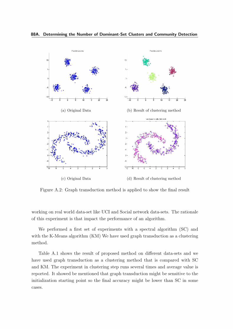
88A. Determining the Number of Dominant-Set Clusters and Community Detection
(a) Original Data (b) Result of clustering method
(c) Original Data (d) Result of clustering method
Figure A.2: Graph transduction method is applied to show the final result
working on real world data-set like UCI and Social network data-sets. The rationale
of this experiment is that impact the performance of an algorithm.
We performed a first set of experiments with a spectral algorithm (SC) and
with the K-Means algorithm (KM) We have used graph transduction as a clustering
method.
Table A.1 shows the result of proposed method on different data-sets and we
have used graph transduction as a clustering method that is compared with SC
and KM. The experiment in clustering step runs several times and average value is
reported. It showed be mentioned that graph transduction might be sensitive to the
initialization starting point so the final accuracy might be lower than SC in some
cases.

A.2. Discussion and future work 89
(a) Three close Gaussians data with high σ
value
(b) Three close dense Gaussians data with
low σ value
Figure A.3: Shows the performance of proposed method on noisy data
A.2 Discussion and future work
We were able to propose an efficient method to detect the number of clusters auto-
matically using the concept of Dominant set approach. We have proved the effec-
tiveness of proposed method in qualitative and quantitative ways by making tests on
different computer generated data sets, UCI repository data sets and social network
data sets and we got an interesting and promising result.
For the future work, we have observed that, there is a growing interest in studying
new algorithms to extract communities allowing a certain degree of overlap between
nodes which can be combined with our work to detect communities without speci-
fying number of clusters in advance.

90A. Determining the Number of Dominant-Set Clusters and Community Detection
Table A.1: The result of proposed method on different data-sets with compression
to SC and KM methods as clustering

Conclusions
In this thesis we presented some of the results that was obtained during my three
years as a Ph.D. student.
C.1 Contributions
The aim of this thesis was to investigate different techniques to compress a graph.
Graph compression is one of the fundamental methods to these days research as far
as the amount of data is increasing rapidly. Graph compression can be utilized in
many environments such as saving the memory space by compressing data. There-
fore, the compression can be lossy or lossless depend on the technique.
Extremal Graph theory is a new branch in graph theory which is developed
during early 20th century. One of the most practical theorem in Extremal Graph
Theory is Szemeredi’s Regularity Lemma which is used in celebrated proof of the
Erdos-Turan Conjecture on arithmetic progressions in dense sets of integers. We
have explored its power in the fields of Pairwise Clustering.
Roughly speaking, the Lemma guarantees the existence, for a sufficiently large
graph, vertices of the graph can be partitioned to the small sub-graphs with equal
size that satisfies particularly strict constraints on the edge density between each
pair of subsets.
We have implemented a two steps strategy method based on Alon et al. [3] work
who presented a first algorithmic method of the Szemeredis Regularity Lemma to
make partition of vertices of an input graph in section III. This partitioning shows
some interesting properties that can be useful for compression in a clustering con-
text. This nature of partitioning can be applied to every graph to partition them.
We have been able to use this method as pre-step clustering method and we have
tested on different benchmark in UCI dataset. Moreover in practice, we had been
able to justify that reduce graph is able to detect a significant sub-structure in orig-

92 Conclusions
inal graph as well as theory. This method is less sensitive to parameter variation
and we were able to show that with changing the compression rate the performance
does not vary much with using Dominant set, as the clustering method. Moreover,
with applying SRL as a preprocessing for dominantset clustering, by increasing the
size of original graph, the time efficiency of our method gets clearer.
We have proposed a novel matrix factorization method as a second technique in
section IV for graph and kernel compression. We have tested our proposed method
on different scenarios like link prediction in the presence of missing observations.
We came up with an update rule which resembles the ones adopted for NMF and
the one introduced by Baum and Eagon for maximizing polynomials with nonneg-
ative coefficients in probability domain. We have proven convergence properties of
these update rules. Our graph compression can be potentially employed to speed-up
existing graph-based and kernel-based algorithms however it was not our focus to
show the effectiveness of our graph compression formulation. However, the experi-
ments conducted in Section 4.7.2 evidenced that the information preserved by the
compression is sufficient to avoid drastic decay of the algorithm’s performances. Ac-
tually, we experienced a constant performance even at low compression rates. The
complexity of many algorithms can be reduced by replacing G with the factorization
X>RX and by exploiting the sparsity of X. As an example, the complexity of a
matrix-vector multiplication can be reduced from n2 to (k2+n). However, for this to
become a real benefit we have to reduce the complexity of the compression algorithm.
We have proposed a two steps method to estimate the number of cluster which is
presented in appendix V. Based on the Motzkin-Straus theorem, they were able to
show a connection between clique number (ω(G)) and the global optimal value of a
certain quadratic function over the standard simplex. We have extended their result
to the weighted case by designing a two steps method to determine the number of
clusters. In the first step, we use dissimilarity matrix as an input and by minimizing
it with replicator, we are able to detect the minimum number of clusters based on
our defined stability number. And then, we examine the existence of undetected
cluster based on the idea of ”Efficient-out-of-sample extension of dominant-set clus-
ters” paper. We have proved the performance of our method on several synthetic
and real world benchmarks in UCI and social network dataset.
Comparison of two Compression methods:

Impact and Future Works 93
1. In the contest of clustering, Szemerdi Regularity method cannot be applied
as a compression device and clustering method in the same time because it is
impossible to think about a clustering procedure that forces all the clusters
to have the same cardinality and another reason is this method cant produce
a good grouping because of its nature that doesnt consider inter- similarity.
In the other hand MFA method can be used as clustering method as we have
shown in section. The main reason is based on the grouping strategy of its
nature.
2. The SLR method can be applied to a large graph as its nature but MFAmethod
it is not very efficient for the large graph. It is computationally expensive
because iterative optimization procedure.
3. In SLR method focuses on inter-sets edges in its nature, while nothing has been
said about intra-subset connections. In the case of MFA, it focuses in both
inter and intra connection. In another words, in classical graph clustering,
vertices that are well connected with each other are grouped together like
MFA method, whereas in a regular decomposition, members of a group have
stochastically similar relations to all other groups. In fact, the internal edge
structure within a group is not considered at all in SRL.
4. Finally, one of cones about are work is we didn’t apply our SRL method in
different applications. Moreover, as far as both methods are lossy, we could
investigate the ability of each method to how much compress and loose infor-
mation for reconstructing back.
C.2 Impact and Future Works
To improve MFA approach to become a real benefit we have to reduce the complexity
of the compression algorithm. To this end, a future direction of research is to exploit
randomized algorithms for speeding-up the factorization and thus the compression
step.
As future works we plan also to consider other types of Bregman divergences
in the objective of (4.3), rather than simply `2 divergence. Another intriguing

94 Conclusions
direction of research consists in investigating generalizations or characterizations of
the multiplicative update rule that we proposed in this thesis.
Finally, another interesting development of our method that we leave to future
research consists in selecting automatically an optimal compression rate. This can
be achieved by imposing a Occam’s razor prior on the model complexity, which
favours simple models (smaller values of k) as opposed to complex ones.

Bibliography
[1] Micah Adler and Michael Mitzenmacher. Towards compressing web graphs.
In In Proc. of the IEEE Data Compression Conference (DCC, pages 203–212,
2000.
[2] Edoardo M. Airoldi, David M. Blei, Stephen E. Fienberg, and Eric P. Xing.
Mixed Membership Stochastic Blockmodels. J. Mach. Learn. Res., 9:1981–
2014, 2008.
[3] N. Alon, R. A. Duke, H. Lefmann, V. Rodl, and R. Yuster. The algorithmic
aspects of the regularity lemma. Journal of Algorithms, 16(1):80 – 109, 1994.
[4] Noga Alon and Raphael Yuster. AlmostH -factors in dense graphs. Graphs and
Combinatorics, 8(2):95–102, 1992.
[5] L. E. Baum and J. A. Eagon. An inequality with applications to statistical
estimation for probabilistic functions of Markov processes and to a model for
ecology. Bull. Amer. Math. Soc., 73:360–363, 1967.
[6] E.M.L. Beale. Euclidean Cluster Analysis. Scientific Control Systems Limited,
1969.
[7] D. M. Blei, A. Y. Ng, and M. I. Jordan. Latent Dirichlet allocation. J. Machine
Learning Research, 3:993–1022, 2003.
[8] Bela Bollobas. Extremal Graph Theory. Dover Publications, Incorporated, 2004.
[9] I. Bomze, M. Pelillo, and V. Stix. Approximating the maximum weight clique
using replicator dynamics. IEEE Trans. Neural Networks, 11:1228–1241, 2000.
[10] Immanuel M. Bomze. Evolution towards the maximum clique. J. of Global
Optimization, 10(2):143–164, March 1997.
[11] D. Cai, X. He, J. Han, and T. S. Huang. Graph regularized nonnegative matrix
factorization for data representation. IEEE Trans. Patt. Analysis Machine
Intell., 33(8):1548–1560, 2011.

96 Bibliography
[12] T. Calinski and J. Harabasz. A dendrite method for cluster analysis. Commu-
nications in Statistics-Simulation and Computation, 3(1):1–27, 1974.
[13] Y. Choi and W. Szpankowski. Compression of graphical structures: Funda-
mental limits, algorithms, and experiments. IEEE Trans. Information Theory,
58(2):620–638, 2012.
[14] Yongwook Choi and Wojciech Szpankowski. Compression of graphical struc-
tures. In IEEE International Symposium on Information Theory, ISIT 2009,
June 28 - July 3, 2009, Seoul, Korea, Proceedings, pages 364–368, 2009.
[15] Thomas H. Cormen, Clifford Stein, Ronald L. Rivest, and Charles E. Leiserson.
Introduction to Algorithms. McGraw-Hill Higher Education, 2nd edition, 2001.
[16] Andrzej Czygrinow and Vojtech Rdl. An algorithmic regularity lemma for
hypergraphs. SIAM J. Comput., 30(4):1041–1066, 2000.
[17] S. Deerwester, S. T. Dumais, G. W. Furnas, T. K. Landauer, and R. Harshman.
Indexing by latent semantic analysis. J. American Soc. for Information Science,
41(6):391–407, 1990.
[18] I. S. Dhillon, Y. Guan, and B. Kulis. Kernel k-means: spectral clustering
and normalized cuts. In Int. Conf. on Knowledge Discovery and Data Mining,
volume 10, pages 551–556, 2004.
[19] Reinhard Diestel. Graph Theory, volume 173 of Graduate Texts in Mathematics.
Springer-Verlag, Heidelberg, third edition, 2005.
[20] C. Ding, X. He, and H. D. Simon. On the equivalence of nonnegative matrix
factorization and spectral clustering. In SIAM Data Mining Conf., pages 606–
610, 2005.
[21] C. Ding, T. Li, and M. I. Jordan. Nonnegative matrix factorization for combi-
natorial optimization: spectral clustering, graph matching and clique finding.
In IEEE Int. Conf. on Data Mining, pages 183–192, 2008.
[22] C. Ding, T. Li, and W. Peng. On the equivalence between non-negative matrix
factorization and probabilistic latent semantic indexing. Comput. Stat. & Data
Analysis, 52(8):3913–3927, 2008.
Bibliography 97
[23] R. O. Duda and P. E. Hart. Pattern Classification and Scene Analysis. John
Willey & Sons, New Yotk, 1973.
[24] Toms Feder and Rajeev Motwani. Clique partitions, graph compression, and
speeding-up algorithms. In STOC’91, pages 123–133, 1991.
[25] Bernd Fischer and Joachim M. Buhmann. Path-based clustering for grouping of
smooth curves and texture segmentation. IEEE TRANSACTIONS ON PAT-
TERN ANALYSIS AND MACHINE INTELLIGENCE, 25(4):513–518, 2003.
[26] A. Frieze. The regularity lemma and approximation schemes for dense problems.
In FOCS ’96: Proceedings of the 37th Annual Symposium on Foundations of
Computer Science, Washington, DC, USA, 1996. IEEE Computer Society.
[27] Alan M. Frieze and Ravi Kannan. The regularity lemma and approxima-
tion schemes for dense problems. In 37th Annual Symposium on Foundations
of Computer Science, FOCS ’96, Burlington, Vermont, USA, 14-16 October,
1996, pages 12–20, 1996.
[28] A. C. Gilbert and K. Levchenko. Compressing network graphs. In Proceedings
of the LinkKDD workshop at the 10th ACM Conference on KDD, August 2004.
[29] Anna Goldenberg, Alice X. Zheng, Stephen E. Fienberg, and Edoardo M.
Airoldi. A survey of statistical network models. Found. Trends Mach. Learn.,
2(2):129–233, 2010.
[30] A.D. Gordon. Classification, 2nd Edition. Chapman & Hall/CRC Monographs
on Statistics & Applied Probability. Taylor & Francis, 1999.
[31] W.T. Gowers. Hypergraph regularity and the multidimensional szemeredi the-
orem. Random Struct. Algorithms, 2004.
[32] Peter D. Grunwald. The Minimum Description Length Principle (Adaptive
Computation and Machine Learning). The MIT Press, 2007.
[33] I. Norros H. Reittu, F. Bazso. A graph compression algorithm inspired by
szemeredis regularity lemma. ArXiv preprint, 2014.
[34] John A. Hartigan. Clustering Algorithms. John Wiley & Sons, Inc., New York,
NY, USA, 99th edition, 1975.

98 Bibliography
[35] Penny E. Haxell, Brendan Nagle, and Vojtech Rodl. An algorithmic version
of the hypergraph regularity method. In 23-25 October 2005, Pittsburgh, PA,
USA, Proceedings, pages 439–448, 2005.
[36] T. Hofmann. Learning the similarity of documents : an information-geometric
approach to document retrieval and categorization. In Advances in Neural
Inform. Process. Syst., volume 12, pages 914–920, 2000.
[37] P. W. Holland, K. B. Laskey, and S. Leinhardt. Stochastic blockmodels: First
steps. Social Networks, 5(2):109–137, 1983.
[38] R. A. Horn and C. R. Johnson. Matrix analysis. Cambridge University Press,
1985.
[39] Tim J. P. Hubbard, Alexey G. Murzin, Steven E. Brenner, and Cyrus Chothia.
SCOP: a structural classification of proteins database for the investigation of
sequences and structures. J. Molec. Biology, 247:536–540, 1995.
[40] Wei Jin and Rohini K. Srihari. Graph-based text representation and knowledge
discovery. In Proceedings of the 2007 ACM Symposium on Applied Computing,
SAC ’07, pages 807–811, New York, NY, USA, 2007. ACM.
[41] I. Jolliffe. Principal Component Analysis. Springer Verlag, 1987.
[42] Hamid Khalili, Amir Yahyavi, and Farhad Oroumchian. Web-graph pre-
compression for similarity based algorithms. In Third International Confer-
ence on Modeling, Simulation and Applied Optimization 2009, Sharjah, U.A.E,
2009, pages 20–22, 2009.
[43] Janos Komlos and Miklos Simonovits. Szemeredi’s regularity lemma and its
applications in graph theory, 1996.
[44] Robert Krauthgamer and Tamar Zondiner. Preserving terminal distances using
minors. CoRR, 2012.
[45] D. Kuang, H. Park, and C. Ding. Symmetric nonnegative matrix factorization
for graph clustering. In SIAM Int. Conf. Data Mining, pages 106–117, 2012.
[46] B. Lakshminarayanan and R. Raich. Non-negative matrix factorization for
parameter estimation in hidden Markov models. In IEEE Int. Workshop on
Machine Learning for Signal Processing, pages 89–94, 2010.
Bibliography 99
[47] D. D. Lee and H. S. Seung. Learning the parts of objects by non-negative
matrix factorization. Nature, 401:788–791, 1999.
[48] D. D. Lee and H. Sebastian Seung. Algorithms for non-negative matrix factor-
ization. In Advances in Neural Inform. Process. Syst., pages 556–562, 2000.
[49] Ping Li, Jiajun Bu, Yi Yang, Rongrong Ji, Chun Chen, and Deng Cai. Dis-
criminative orthogonal nonnegative matrix factorization with flexibility for data
representation. Expert Systems with Applications, 41(4):1283–1293, 2014.
[50] Ping Li, Chun Chen, and Jiajun Bu. Clustering analysis using manifold kernel
concept factorization. Neural Computation, 87:120–131, 2012.
[51] F. Lorrain and H. C. White. Structural equivalence of individuals in social
networks. J. of Math. Sociology, 1:49–80, 1971.
[52] J. Maynard Smith. Evolution and the Theory of Games. Cambridge University
Press, Cambridge, UK, 1982.
[53] Glenn Milligan and Martha Cooper. An examination of procedures for deter-
mining the number of clusters in a data set. Psychometrika, 50(2):159–179,
1985.
[54] M. Mørup and M. Schmidt. Bayesian community detection. Neural Computa-
tion, 24(9):2434–2456, 2012.
[55] T. S. Motzkin and E. G. Straus. Maxima for graphs and a new proof of a
theorem of Turan. Canadian Journal of Mathematics, 17:533–540, 1965.
[56] Theodore S Motzkin and Ernst G Straus. Maxima for graphs and a new proof
of a theorem of turan. Canad. J. Math, 17(4):533–540, 1965.
[57] S. Navlakha, R. Rastogi, and N. Shrivastava. Graph summarization with
bounded error. In ACM SIGMOD Int. Conf. on Management of Data, pages
419–432, 2008.
[58] Tamas Nepusz, Andrea Petroczi, Laszlo Negyessy, and Fulop Bazso. Fuzzy
communities and the concept of bridgeness in complex networks. Phys. Rev. E,
77(1):016107, 2008.

100 Bibliography
[59] F. Nourbakhsh, S. Rota Bulo, and M. Pelillo. A matrix factorization approach
to graph compression. In Int. Conf. Patt. Recogn., 2014.
[60] P. Paatero and A. U. Tapper. Positive matrix factorization: a non-negative
factor model with optimal utilization of error estimates of data values. Envi-
ronmetrics, 5:111126, 1994.
[61] Panos M Pardalos and AT Phillips. A global optimization approach for solving
the maximum clique problem. International Journal of Computer Mathematics,
33(3-4):209–216, 1990.
[62] M. Pavan and M. Pelillo. Dominant sets and hierarhical clustering. In Int.
Conf. Comp. Vision, volume 1, pages 362–369, 2003.
[63] M. Pavan and M. Pelillo. Efficient out-of-sample extension of dominant-set
clusters. Advances in Neural Inform. Process. Syst., 17:1057–1064, 2005.
[64] Massimiliano Pavan and Marcello Pelillo. Graph-theoretic approach to cluster-
ing and segmentation. In 2003 IEEE Computer Society Conference on Com-
puter Vision and Pattern Recognition (CVPR 2003), 16-22 June 2003, Madi-
son, WI, USA, pages 145–152, 2003.
[65] Marcello Pelillo. A unifying framework for relational structure matching. In
Fourteenth International Conference on Pattern Recognition, ICPR 1998, Bris-
bane, Australia, 16-20 August, 1998, pages 1316–1319, 1998.
[66] Marcello Pelillo. Replicator equations, maximal cliques, and graph isomor-
phism. Neural Computation, 11(8):1933–1955, 1999.
[67] Marcello Pelillo. Metrics for attributed graphs based on the maximal similarity
common subgraph. Int. J. Pattern Recognition Artif. Intell, 2004:299–313, 2004.
[68] Marcello Pelillo and Arun Jagota. Feasible and infeasible maxima in a quadratic
program for maximum clique. J. Artif. Neural Networks, 2:411–420, 1995.
[69] I. Psorakis, S. Roberts, M. Ebden, and B. Sheldon. Overlapping community
detection using nonnegative matrix factorization. Phys. Rev. E, 83(6):066114,
2011.
[70] Vojtech Rodl and Jozef Skokan. Applications of the regularity lemma for uni-
form hypergraphs. Random Struct. Algorithms, 28(2):180–194, 2006.

Bibliography 101
[71] Samuel Rota Bulo, Andre Lourenco, Ana L. N. Fred, and Marcello Pelillo.
Pairwise probabilistic clustering using evidence accumulation. In Int. Work. on
Struct. and Synt. Patt. Recogn., pages 395–404, 2010.
[72] Samuel Rota Bulo and Marcello Pelillo. Probabilistic clustering using the baum-
eagon inequality. In Int. Conf. Patt. Recogn., pages 1429–1432, 2010.
[73] Peter Rousseeuw. Silhouettes: A graphical aid to the interpretation and val-
idation of cluster analysis. J. Comput. Appl. Math., 20(1):53–65, November
1987.
[74] L. Samuelson. Evolutionary games and equilibrium selection. MIT Press, Cam-
bridge, MA, 1997.
[75] B. Scholkopf, A. Smola, and K. R. Mller. Nonlinear component analysis as a
kernel eigenvalue problem. Neural Computation, 10(5):1299–1319, 1998.
[76] J. Shi and J. Malik. Normalized cuts and image segmentation. IEEE Trans.
Patt. Analysis Machine Intell., 22:888–905, 2000.
[77] Jianbo Shi and Jitendra Malik. Normalized cuts and image segmentation. IEEE
Transactions on Pattern Analysis and Machine Intelligence, 22:888–905, 1997.
[78] A. Sperotto and M. Pelillo. Szemeredis regularity lemma and its applications to
pairwise clustering and segmentation. In Energy Minim. Methods in Computer
Vision and Patt. Recogn., pages 13–27, 2007.
[79] Torsten Suel and Jun Yuan. Compressing the graph structure of the web. In
Data Compression Conference, DCC 2001, Snowbird, Utah, USA, March 27-29,
2001., pages 213–222, 2001.
[80] E. Szemeredi. Regular partitions of graphs. In Problemes combinatoires et
thorie des graphes, pages 399–401. CNRS, Paris, 1978.
[81] Endre Szemeredi. On sets of integers containing no k elements in arithmetic
progression. ICM: 2nd International Congress of Mathematicians, 1975.
[82] Endre Szemeredi. Regular partitions of graphs. Technical report, Stanford, CA,
USA, 1975.

102 Bibliography
[83] Robert Tibshirani, Guenther Walther, and Trevor Hastie. Estimating the num-
ber of clusters in a dataset via the gap statistic. 63:411–423, 2000.
[84] H. Toivonen, F. Zhou, A. Hartikainen, and A. Hinkka. Compression of weighted
graphs. In Int. Conf. on Knowledge Discovery and Data Mining, pages 965–973,
2011.
[85] Hannu Toivonen, Fang Zhou, Aleksi Hartikainen, and Atte Hinkka. Compres-
sion of weighted graphs. In Proceedings of the 17th ACM SIGKDD international
conference on Knowledge discovery and data mining, KDD ’11, pages 965–973,
New York, NY, USA, 2011. ACM.
[86] D. Verma and M. Meila. Comparison of spectral clustering methods. Technical
report, University of Washington, 2003.
[87] W. Xu and Y. Gong. Document clustering by concept factorization. In Proc. of
27th annual international ACM SIGIR conference on Research and development
in information retrieval, pages 202–209, 2004.
[88] Mingjin Yan. Methods of Determining the Number of Clusters in a Data Set
and a New Clustering Criterion. PhD thesis, Virginia Polytechnic Institute and
State University,Blacksburg, Virginia, 2005.
[89] Z. Yang and E. Oja. Quadratic nonnegative matrix factorization. Pattern
Recogn., 45(4):1500–1510, 2012.
[90] H. Zhang, Z. Yang, and E. Oja. Adaptive multiplicative updates for quadratic
nonnegative matrix factorization. Neural Computation, 134:206–213, 2014.