algorithms for enumerating all spanning trees of undirected and weighted graphs presented by...
TRANSCRIPT

Algorithms for Enumerating All Spanning Trees of Undirected and Weighted Graphs
Presented by
R97922102 李孟哲R97922104 陳翰霖R97922124 張仕明
Sanjiv Kapoor and H.Ramesh

Index
• Introduction
• Computation Tree
• Algorithm 1
• Algorithm 2
• Algorithm 3

Introduction
• Spanning tree enumeration in undirected graphs is an important issue in network and circuit analysis
• In this paper, author enumerate spanning trees by the computation tree
• Every node in the computation tree represent a spanning tree

Algorithms Introduction
• We use this way to enumerate all the spanning tree on undirected and weighted graphs.
• Algorithm 1– O(N+V+E) time– O(V2E) space
• Algorithm 2– O(N+V+E) time– O(VE) space
• Algorithm 3 (with sorting)– O(NlogV+VE) time– O(N+VE) space

Spanning Tree
• The original graph G

Spanning Tree
• A Spanning tree of G

Spanning Tree
• add a edge to the tree

Spanning Tree
• get a cycle (fundamental cycle)

Spanning Tree
• remove a edge on the cycle

Spanning Tree
• get a new spanning tree of G

Spanning Tree
• From this cycle, we can obtain several spanning trees.

Computation Tree

Computation tree
• First, we start off with a spanning tree T, and generate all other spanning trees form T by replacing edges in T by edges outside T
• For every node x, Sx is the spanning tree corresponding to this node
• To ensure that each spanning tree is generated exactly once, we use 2 edge set INx and OUTx for every node x

IN and OUT
• The set INx consist of edges which are always included in node x and it’s descendants
• The set OUTx consist of edges which are always not included in node x and it’s descendants
• The IN and OUT set of the root are both empty

Computation tree
1
2 3 4
51
2 3 4
5
In =[ ] Out=[ ] S =[ ]
, , 1,2,4
Arbitrary choose a spanning tree

Computation tree
1
2 3 4
5
1
2 3 4
5
In =[ ] Out=[ ] S =[ ]
, , 1,2,4

Computation tree
1
2 3 4
5
1
2 3 4
5
In =[ ] Out=[ ] S =[ ]
, , 1,2,4
In =[ ] Out=[ ] S =[ ]
, , ,
In =[ ] Out=[ ] S =[ ]
, , ,
In =[ ] Out=[ ] S =[ ]
, , ,
In =[ ] Out=[ ] S =[ ]
, , ,

Computation tree
1
2 3 4
5
1
2 3 4
5
In =[ ] Out=[ ] S =[ ]
, , 1,2,4
In =[ ] Out=[ ] S =[ ]
, , 2,4,5
In =[ ] Out=[ ] S =[ ]
, , 1,2,5
In =[ ] Out=[ ] S =[ ]
, , 1,2,4
In =[ ] Out=[ ] S =[ ]
, , 1,4,5
1
2 3 4
5
1
2 3 4
5
1
2 3 4
5
1
2 3 4
5
(-2,+5)
(-1,+5)
(-4,+5)

Computation tree
1
2 3 4
5
1
2 3 4
5
In =[ ] Out=[ ] S =[ ]
, , 1,2,4
In =[ ] Out=[ ] S =[ ]
, 1, 2,4,5
In =[ ] Out=[ ] S =[ ]
, 4, 1,2,5
In =[ ] Out=[ ] S =[ ]
, 5, 1,2,4
In =[ ] Out=[ ] S =[ ]
, 2, 1,4,5
1
2 3 4
5
1
2 3 4
5
1
2 3 4
5
1
2 3 4
5
(-2,+5)
(-1,+5)
(-4,+5)

Computation tree
1
2 3 4
5
1
2 3 4
5
In =[ ] Out=[ ] S =[ ]
, , 1,2,4
In =[ ] Out=[ ] S =[ ]
5, 1, 2,4,5
In =[ ] Out=[ ] S =[ ]
5, 4, 1,2,5
In =[ ] Out=[ ] S =[ ]
, 5, 1,2,4
In =[ ] Out=[ ] S =[ ]
5, 2, 1,4,5
1
2 3 4
5
1
2 3 4
5
1
2 3 4
5
1
2 3 4
5
(-2,+5)
(-1,+5)
(-4,+5)

Computation tree
1
2 3 4
5
1
2 3 4
5
In =[ ] Out=[ ] S =[ ]
, , 1,2,4
In =[ ] Out=[ ] S =[ ]
5,2, 1, 2,4,5
In =[ ] Out=[ ] S =[ ]
5,2,1, 4, 1,2,5
In =[ ] Out=[ ] S =[ ]
, 5, 1,2,4
In =[ ] Out=[ ] S =[ ]
5, 2, 1,4,5
1
2 3 4
5
1
2 3 4
5
1
2 3 4
5
1
2 3 4
5
(-2,+5)
(-1,+5)
(-4,+5)

Computation tree
1
2 3 4
5
1
2 3 4
5
In =[ ] Out=[ ] S =[ ]
, 5, 1,2,4

Computation tree
1
2 3 4
5
1
2 3 4
5
In =[ ] Out=[ ] S =[ ]
, 5, 1,2,4
In =[ ] Out=[ ] S =[ ]
, 5, 1,3,4
In =[ ] Out=[ ] S =[ ]
, 5,3 1,2,4
In =[ ] Out=[ ] S =[ ]
, 5, 2,3,4
1
2 3 4
5
1
2 3 4
5
1
2 3 4
5
(-1,+3)
(-2,+3)

Computation tree
1
2 3 4
5
1
2 3 4
5
In =[ ] Out=[ ] S =[ ]
, 5, 1,2,4
In =[ ] Out=[ ] S =[ ]
1,3, 5,2 1,3,4
In =[ ] Out=[ ] S =[ ]
, 5,3 1,2,4
In =[ ] Out=[ ] S =[ ]
3, 5,1 2,3,4
1
2 3 4
5
1
2 3 4
5
1
2 3 4
5
(-1,+3)
(-2,+3)

Computation tree
1
2 3 4
5

Computation tree C’(G)

Appear not only once
• The last son and its parent are the same

Another Computation tree C’(G)
1
2 3 4
5
G
C(G) C’(G)

Another Computation tree C’(G)

Computation tree C(G)’s property
• The son has zero or one edge differ from its parent.
• The number of sons equals to the length of the fundamental cycle

Computation tree C’(G)’s property
• The son has one edge differ from its parent.• The number of sons equals to the sum of the
length of all fundamental cycles

Lemma 1
• The computation tree has at its internal nodes and leaves all the spanning trees of G
• [Proof] • Following from induction and inclusion/exclusion
principle• Let A be a node of computation tree C(G),
B1,...,Bk+1 be the son of A

• All spanning trees in B1,…, Bk contain edge f
• All spanning trees in Bk+1 don’t contain edge f
• The spanning trees as Bj ‘s descendants contain edges e1,…,ej-1, but the edge ej
• e1,…,ek and f form a cycle
A
B1 B2 Bk Bk+1…
… … … …computation tree
f
e1
e2
ek

Algorithm 1

The Algorithm 1
…
Generate a random spanning tree and initialize some data structures.
Prepare and modify the data structures.
Recursively call the algorithm.

Possible problem in algorithm
• How to maintain the IN , OUT, S ?• How to find the fundamental cycles?

Possible problem in algorithm
• How to maintain the IN , OUT, S ?– S is easy, just add a edge and delete another one.– We use a data structure AG to maintain IN, OUT.– We would choose edges from AG
– Initial: AG is the graph itself.

Possible problem in algorithm
– Modify AG – Adding a edge into IN– Contract the edge
12
3
12
3

Possible problem in algorithm
– Modify AG – Add a edge into OUT– Delete the edge
12
3
12
3

Modify the fundamental cycle
• After we exchange the edges, the fundamental cycles of this tree would change
• We need to modify the fundamental cycles
f
e1 e2
e3
f
e1
e3
e2
f
e1
e3
e2

Modify the fundamental cycle
• Author uses the data structure C to maintain the fundamental cycles
• C maintains the fundamental cycles corresponding to the current tree
• There are 3 operations to construct computation tree:1. After deleting edge ei in AG, merge the fundamental
cycles contain ei
2. After contracting edge e in AG, contract edge e in C
3. Delete the nontree edge for the last son
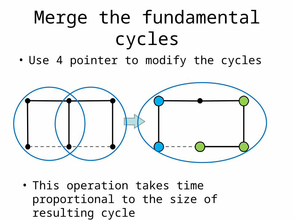
Merge the fundamental cycles
• Use 4 pointer to modify the cycles
• This operation takes time proportional to the size of resulting cycle

Contract edge in C
• This operation takes time proportional to fundamental cycles containing the contracted edge

Delete the nontree edge in C
• If the nontree edge is a part of a multiedge, then do nothing
• else delete the fundamental cycle containing the nontree edge
• This operation takes time proportional to the size of its fundamental cycle

AG and C
• When some edge e is added to set IN:– Contract e in AG and C
• When some edge e is added to set OUT:– Delete e in AG and C – Merge the fundamental cycles containing e

Lemma 1.2
• The algorithm done at each node A of C(G) is O(|s(A)|+|g(A)|)
• Where s(A) is the set of sons of A in C(G), g(A) is the set of sons in C’(G) of nodes in s(A)

Proof
• When replace tree edge ei by f , We need to
– Contract f in AG: constant time
– merge fundamental cycles in C containing ei:it takes time proportional to the sum size of resulting cycle ( O(|g(A)|) )
– Contract ei in C: it takes time proportional to the number of cycles contain ei ( O(|g(A)|) )
– Contract ei in AG:
it takes time proportional to the number of multiedges incident to the endpoints of ei ( O(|g(A)|) )

Proof
• Before operating the node is the last son, then – Delete f in AG:
constant time – Delete f in C:
time proportional to the size of its fundamental cycle( O(s(A)) )
• Every node takes O(|s(A)|+|g(A)|) time

Theorem 1.3
• All spanning trees can be correctly generated in O( N + V + E ) time by Algorithm 1
• [Proof]– First, construct a spanning tree and setup it’s
data structure• require O( V + E ) time
– Every node in computation tree C(G) takes O(|s(A)|+|g(A)|) time
– Summing overall nodes of C(G) is O(N)

Theorem 1.4
• The space requirement of the spanning tree enumeration Algorithm 1 is O( V2E )
• [Proof]– At each node of C(G), take O( VE ) space– The height of C’(G) is at most V
…
… …

Algorithm 2

Algorithm 2
• We play two tricks to reduce the space complexity from O(V2E) to O(VE) – DFS tree– Biconnected components

DFS tree
• The first spanning tree is generated by depth first search.– Nontree edges are back edges
• It is easy to find the fundamental cycle of the depth first search tree

Why it’s easier at DFS tree
• To find a fundamental cycle, we just need to trace the back edge
• We can reduce the space requirement since we don’t have to maintain the fundamental cycle set

Maintaining the d.f.s invariant
• For a node A of C(G), SA is a d.f.s tree of GA
• Assume the vertices of SA are numbered by a post-order traversal
1
23
45
6
7
8root

Maintaining the d.f.s invariant
• Select the nontree edge whose upper endpoint has the smallest number (upper is the endpoint closer to the root)
• This edge is the replacement edge
1
23
45
6
7
8root

Maintaining the d.f.s invariant
• Replace the tree in order of the post-order number
• The new graph’s spanning tree is still a d.f.s tree
1
23
45
6
7
8 1
23
45
6
7
81
23
5
6
7
8

Biconnected components

Biconnected components
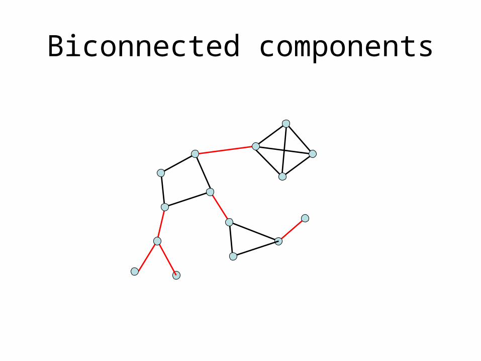
Biconnected components

Biconnected components
• The red edges (bridges) must be chosen in each spanning tree of G.
• Let nST(G) be the number of spanning trees in G.
• Then nST(G) = nST(G1)*nST(G2)*…..nST(Gn)
G1
G2
G3
G4
G5

Biconnected components
• No change in time and space complexity in analysis, but make the algorithm efficiency in most cases.

Bridge
• When exchange edges, there may be some tree edges which is not contained by any fundamental cycles– We call those edges bridges– A bridge must be in this spanning tree

How to detect bridge
• Bridge only occurs on a fundamental cycle when we exchange 2 edges
• Since x4 has a branch in current graph GA ,e4 is a bridge when we delete e3
e1
e2
e4
e5
e3
x4
Lemma 2.1
• The work done at each node A of C(G) is O(|s(A)|+|g(A)|)
• Proof : – Removing bridges spends time in O(|s(A)|)– Exchanging and contracting edges spend
O(g|A|)

Theorem 2.2
• All spanning tree can be correctly generated in O( N + V + E ) time by Algorithm 2
• [Proof]– First, we construct a spanning and setup it’s
data structure • require O( V + E ) time
– Every node in computation tree C(G) takes O(|s(A)|+|g(A)|) time
– Summing overall nodes of C(G) takes O(N) time

Theorem 2.3
• The space requirement in Algorithm 2 is O( VE )• [Proof]
– At each node of C(G), takes O( E ) space– The height of C’(G) is at most V
…
… …

Algorithm 3

Algorithm 3
• If we want to show all the spanning trees in increasing order.– Generate all the trees O(N+V+E)– Sorting all the trees O(NlogN)
• Algorithm 3 generates sorted order in O(NlogV+VE)time

Algorithm 3
• We create M queues, M = (V-1)(E-V+1)=O(VE) and indexed by “exchange”
…

Algorithm 3
• We create a priority queue (heap) whose size is equal to M=O(VE), and height is O(logVE)
• This heap maintains the first element of each queue.
…
….

Algorithm 3
…
We sort all the nontree edges by increasing order.

Algorithm 3
…
Minimum spanning tree
Output this one

Algorithm 3
…
Add the smallest nontree edge and delete a tree edge.
We can generate the sons

Algorithm 3
… Insert these nodes into queue corresponding to “exchange”

Algorithm 3
…Get the minimum cost tree from the heap.
Output this tree.
Do the algorithm again
….

Algorithm 3
…Insert these nodes into queues corresponding to “exchange”

Algorithm 3
…
We choose the minimum cost tree from the heap again,
These blue vertices are possible to be chosen.

Analysis of algorithm 3
• [Lemma 3.1] Any child’s cost is larger than parent’s.
…
Tree edges = {e1,e2….en}
Nontree edges = {f1,f2…..fm}
This node’s cost must be larger than( or equal to) parent’s.

Analysis of algorithm 3
• [Lemma 3.1] Any child’s cost is larger than parent’s.
…
Tree edges = {e1,e2….en}U{f1}
Nontree edges = {f2…..fm}
This node’s cost must be larger than( or equal to) parent’s.

Analysis of algorithm 3
• [Lemma 3.2] The spanning trees enter the queue for each of the exchanges in sorted order.
• Blue one is smaller than red one.
…

Analysis of algorithm 3
• Those two nodes are in queue, which implies their parents have been output.
• Blue one is in front, because its parent outputs earlier than dark red one.
• Because they have same “exchange”, so blue one < red one. …

Analysis of algorithm 3
• Time complexity– Sorting edges: O(ElogE) time– Generation: O(N+V+E) time– O(VE) queues, N trees– Create a heap: O(VE) time.– One operation in heap: O(logVE) time– N operation in heap: O(NlogVE) time
– O(N logVE) + O(ElogE) + O(N+V+E) + O(VE)
=O(N logV3 + ElogE + N + V + E + VE)
=O( N logV + VE)

Analysis of algorithm 3
• Space complexity– O(N) trees– O(VE) queues
– O(N+VE) space