algorithms and data structures - hu-berlin.de and data structures ulf leser open hashing . ... •...

Algorithms and Data Structures

Ulf Leser

Open Hashing

Ulf Leser: Alg&DS, Summer Semester 2015 2

Open Hashing

• Open Hashing: Store all values inside hash table A • Inserting values

– No collision: Business as usual – Collision: Chose another index and probe again (is it “open”?) – As second index might be full as well, probing must be iterated

• Many suggestions on how to chose the next index to probe • In general, we want a strategy (probe sequence) that

– … ultimately visits any index in A (and few twice before) – … is deterministic – when searching, we must follow the same

order of indexes (probe sequence) as for inserts


Reaching all Indexes of A

• Definition Let A be a hash table, |A|=m, over universe U and h a hash function for U into A. Let I={0, …, m-1}. A probe sequence is a deterministic, surjective function s: UxI→I

• Remarks – We use j to denote elements of the sequence: Where to jump after

j-1 probes – s need not be injective – a probe sequences may cross itself

• But it is better if it doesn’t

– We typically use s(k, j) = (h(k) – s’(k, j)) mod m for a properly chosen function s’

• Example: s’(k, j) = j ,hence s(k, j) = (h(k)–j) mod m


Searching

• Let s’(k, 0) := 0 • We assume that s cycles

through all indexes of A – In whatever order

• Probe sequences longer than m-1 usually make no sense, as they necessarily look into indexes twice – But beware of non-injective

functions

1. func int search(k int) { 2. j := 0; 3. first := h(k); 4. repeat 5. pos := (first-s’(k, j) mod m; 6. j := j+1; 7. until (A[pos]=k) or

(A[pos]=null) or (j=m); 8. if (A[pos]=k) then 9. return pos; 10. else 11. return -1; 12. end if; 13.}


Deletions

• Deletions are a problem – Assume h(k)= k mod 11 and s(k, j) = (h(k) + 3*j) mod m)

1 6 ins( 1); ins(6)

ins( 23)

ins( 12)

del( 23)

search( 12)

0 1 2 3 4 5 6 7 8 9 10

1 23 6

1 23 6 12

1 6 12

1 ? 6 12


Remedies

• Leave a mark (tombstone) – During search, jump over tombstones – During insert, tombstones may be replaced

• Re-organize list – Keep pointer p to index where a key should be deleted – Walk to end of probe sequence (first empty entry) – Move last non-empty entry to index p – Requires to run through the probe entire sequence for every

deletion (otherwise only n/2 on average) – Not compatible with strategies that keep probe sequences sorted

• See later


Open versus External collision handling

• Pro – We do not need more space than reserved – more predictable – A typically is filled more homogeneously – less wasted space

• Contra – More complicated – Generally, we get worse WC/AC complexities for insertion/deletion

• Additional work to run down probe sequences • Especially deletions have overhead

– A gets full; we cannot go beyond α=1


Open Hashing: Overview

• We will look into three strategies – Linear probing: s( k, j) := (h(k) – j) mod m – Double hashing: s( k, j) := (h(k) – j*h’(k)) mod m – Ordered hashing: Any s; values in probe sequence are kept sorted

• Others – Quadratic hashing: s( k, j) := (h(k) – floor(j/2)2*(-1)j) mod m

• Less vulnerable to local clustering then linear hashing

– Uniform hashing: s is a random permutation of I dependent on k • High administration overhead, guarantees shortest probe sequences

– Coalesced hashing: s arbitrary; entries are linked by add. pointers • Like overflow hashing, but overflow chains are in A; needs additional

space for links


Content of this Lecture

• Open Hashing – Linear Probing – Double Hashing – Ordered Hashing


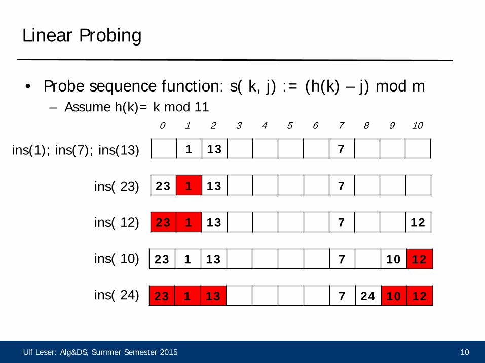
Linear Probing

• Probe sequence function: s( k, j) := (h(k) – j) mod m – Assume h(k)= k mod 11

1 13 7

23 1 13 7

ins(1); ins(7); ins(13)

ins( 23)

ins( 12)

ins( 10)

ins( 24)

23 1 13 7 12

23 1 13 7 10 12

23 1 13 7 24 10 12

0 1 2 3 4 5 6 7 8 9 10


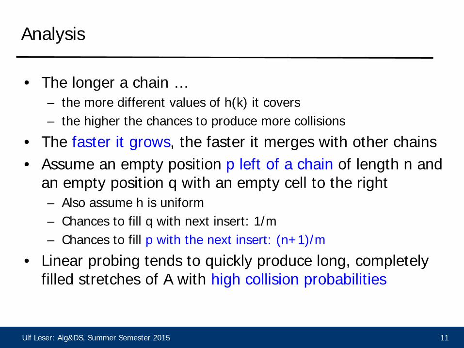
Analysis

• The longer a chain … – the more different values of h(k) it covers – the higher the chances to produce more collisions

• The faster it grows, the faster it merges with other chains • Assume an empty position p left of a chain of length n and

an empty position q with an empty cell to the right – Also assume h is uniform – Chances to fill q with next insert: 1/m – Chances to fill p with the next insert: (n+1)/m

• Linear probing tends to quickly produce long, completely filled stretches of A with high collision probabilities


In Numbers (Derivation of Formulas Skipped)

Source: S. Albers / [OW93]

• Scenario: Some inserts, then many searches – Expected number of probes per search are most important


Quadratic Hashing

Source: S. Albers / [OW93]


Discussion

• Disadvantage of linear (and quadratic) hashing:

Problems with the original hash function h are preserved – Probe sequence only depends on h(k), not on k

• s’(k, j) ignores k

– All synonyms k, k’ will create the same probe sequence • Two keys that form a collision are called synonyms

– Thus, if h tends to generate clusters (or inserted keys are non-uniformly distributed in U), also s tends to generate clusters (i.e., sequences filled from multiple keys)


Double Hashing

• Double Hashing: Use a second hash function h’ – s( k, j) := (h(k) – j*h’(k)) mod m (with h’(k)≠0) – Further, we don’t want that h’(k)|m (done if m is prime)

• h’ should spread h-synonyms – If h(k)=h(k’), then hopefully h’(k)≠h’(k’)

• Otherwise, we preserve problems with h

– Optimal case: h’ statistically independent of h, i.e., p(h(k)=h(k’)∧h’(k)=h’(k’)) = p(h(k)=h(k’))*p(h’(k)=h’(k’))

• If both are uniform: p(h(k)=h(k’)) = p(h’(k)=h’(k’)) = 1/m

• Example: If h(k)= k mod m, then h’(k)=1+k mod (m-2)


Example (Linear Probing produced 9 collisions)

h(k) = k mod 11; h‘(k)= 1+k mod 9; s(k,j) := (h(k)– j*h’(k)) mod 11

ins(23) h(k)=1; h‘(k)=6

s(k, 1)=6

ins( 12) h(k)=1; h‘(k)=4

s(k, 1)=8

ins( 10)

ins( 24) h(k)=2; h‘(k)=7

s(k, 1)=6 s(k, 2)=10 s(k, 3)=3

ins(1); ins(7); ins(13) 1 13 7

1 13 23 7

1 13 23 7 12

1 13 23 7 12 10

1 13 24 23 7 12 10

0 1 2 3 4 5 6 7 8 9 10


Analysis

• Please see [OW93]


Another Example

ins(34) h(k)=1; h‘(k)=8

s(k, 1)=4

ins( 12) h(k)=1; h‘(k)=4

s(k, 1)=8

ins( 10)

ins( 15) h(k)=4; h‘(k)=7

s(k, 1)=8 s(k, 2)=1 s(k,3)=5

ins(23); ins(13) 23 13

23 13 34

23 13 34 12

23 13 34 12 10

23 13 34 15 12 10

0 1 2 3 4 5 6 7 8 9 10


Observation

• We change the order of insertions (and nothing else)

ins(15) h(k)=4; h‘(k)=6

ins( 12) h(k)=1; h‘(k)=4

s(k, 1)=8

ins( 10)

ins( 34) h(k)=1; h‘(k)=8

s(k, 1)=4 s(k, 2)=7

ins(23); ins(13) 23 13

23 13 15

23 13 15 12

23 13 15 12 10

23 13 15 34 12 10


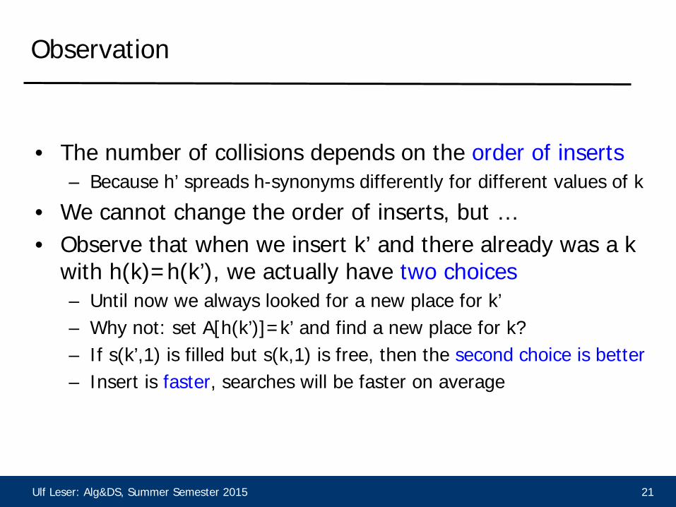
Observation

• The number of collisions depends on the order of inserts

– Because h’ spreads h-synonyms differently for different values of k

• We cannot change the order of inserts, but … • Observe that when we insert k’ and there already was a k

with h(k)=h(k’), we actually have two choices – Until now we always looked for a new place for k’ – Why not: set A[h(k’)]=k’ and find a new place for k? – If s(k’,1) is filled but s(k,1) is free, then the second choice is better – Insert is faster, searches will be faster on average


Brent’s Algorithm Brent, R. P. (1973). "Reducing the Retrieval Time of Scatter Storage Techniques." CACM

• Brent’s algorithm:

Upon collision, propagate key for which the next index in probe sequence is free; if both are occupied, propagate k’

• Improves only successful searches – Otherwise we have to follow the chain to its end anyway

• One can show that the average-case probe length for successful searches now is constant (~2.5 accesses) – Even for relatively full tables


Idea

• Can we do something to improve unsuccessful searches?

– Recall overflow hashing: If we keep the overflow chain sorted, we can stop searching after α/2 comparisons on average

• Transferring this idea: Keep keys sorted in any probe seq. – We have seen with Brent’s algorithm that we have the choice

which key to propagate whenever we have a collision – Thus, we can also choose to always propagate the larger of both

keys – which generates a sorted probe sequence

• Result: Unsuccessful are as fast as successful searches


Details

• In Brent‘s algorithm, we only replace a key if we can insert

the replaced key directly into A • Now, we must replace keys even if the next slot in the

probe sequence is occupied – We run through probe sequence until we meet a key that is smaller – We insert the new key here – All subsequent keys must be replaced (moved in probe sequence)

• Note that this doesn’t make inserts slower than before – Without replacement, we would have to search the first free slot – Now we replace until the first free slot


Critical Issue

– Imagine ins(6) would first probe position 1, then 4 – Since 6<9, 9 is replaced; imagine the next slot would be 8 – Since 9<14, 14 is replaced

• Problem

– 14 is not a synonym of 9 – two probe sequences cross each other – Thus, we don’t know where to move 14 – the next position in

general requires to know the “j”, i.e., the number of hops that were necessary to get from h(14) to slot 8

• Ordered hashing only works if we can compute the next offset without knowing j – E.g. linear hashing (offset -1) or double hashing (offset –h‘(k))

3 2 9 14

3 2 6 9 14


Correctness

• Invariant: Let s(k,j) be the position in A where k is stored.

Searching k returns the correct answer iff ∀i<j: A[s(k,i)] < A[s(k,j)]

• Proof by induction – Invariant holds for the empty array – Imagine invariant holds before inserting a key k’ – We insert k’ in position s(k’,j) (for some j)

• Either A[s(k’,j)] was free – then invariant still holds

• Or the old A[s(k’,j)]<k’ (otherwise we wouldn’t have inserted k’ here) – Then the old A[s(k’,j)] was replaced by a smaller value – Invariant must still hold


Wrap-Up

• Open hashing can be a good alternative to overflow

hashing even if the fill grade approaches 1 – Very little average-case cost for look-ups with double hashing and

Brent’s algorithm or using ordered hashing • Depending which types of searches are more frequent

• Open hashing suffers from having only static place, but guarantees to not request more space once A is allocated – Less memory fragmentation


Exemplary Questions

• Create a hashtable step-by-step using open hashing with double probing and hash functions h(k)=k mod 13 and h’(k)=3+k mod 9 when inserting keys 17,12,4,1,36,25,6

• Use the same list for creating a hash table with double hashing and Brent’s algorithm

• Use the same list for creating a hash table with ordered linear probing (linear probing such that the probe sequences are ordered).

• Analyze the WC complexity of searching key k in a hash table with direct chaining using a sorted linked list when (a) k is in A; (b) k is not in A.

algorithms and data structures - hu-berlin.de and data structures ulf leser open hashing . ... •...

Documents