algorithmica - carnegie mellon school of computer scienceguyb/papers/delaunay99.pdf · algorithmica...
TRANSCRIPT
Algorithmica (1999) 24: 243–269 Algorithmica© 1999 Springer-Verlag New York Inc.
Design and Implementation of a Practical ParallelDelaunay Algorithm1
G. E. Blelloch,2 J. C. Hardwick,3 G. L. Miller,2 and D. Talmor4
Abstract. This paper describes the design and implementation of a practical parallel algorithm for Delau-nay triangulation that works well on general distributions. Although there have been many theoretical parallelalgorithms for the problem, and some implementations based on bucketing that work well for uniform distribu-tions, there has been little work on implementations for general distributions. We use the well known reductionof 2D Delaunay triangulation to find the 3D convex hull of points on a paraboloid. Based on this reductionwe developed a variant of the Edelsbrunner and Shi 3D convex hull algorithm, specialized for the case whenthe point set lies on a paraboloid. This simplification reduces the work required by the algorithm (number ofoperations) fromO(n log2 n) to O(n logn). The depth (parallel time) isO(log3 n) on a CREW PRAM. Thealgorithm is simpler than previousO(n logn) work parallel algorithms leading to smaller constants.
Initial experiments using a variety of distributions showed that our parallel algorithm was within a factor of 2in work from the best sequential algorithm. Based on these promising results, the algorithm was implementedusing C and an MPI-based toolkit. Compared with previous work, the resulting implementation achievessignificantly better speedups over good sequential code, does not assume a uniform distribution of points, andis widely portable due to its use of MPI as a communication mechanism. Results are presented for the IBMSP2, Cray T3D, SGI Power Challenge, and DEC AlphaCluster.
Key Words. Delaunay triangulation, Parallel algorithms, Algorithm experimentation, Parallel imple-mentation.
1. Introduction. A Delaunay triangulation inR2 is the triangulation of a setSof pointssuch that there are no elements ofS within the circumcircle of any triangle. Delaunaytriangulation—along with its dual, the Voronoi Diagram—is an important problem inmany domains, including pattern recognition, terrain modeling, and mesh generation forthe solution of partial differential equations. In many of these domains the triangulationis a bottleneck in the overall computation, making it important to develop fast algo-rithms. As a consequence, there are many sequential algorithms available for Delaunaytriangulation, along with efficient implementations. Su and Drysdale [1] present an ex-cellent experimental comparison of several such algorithms. Since these algorithms aretime and memory intensive, parallel implementations are important both for improvedperformance and to allow the solution of problems that are too large for sequential ma-chines. However, although several parallel algorithms for Delaunay triangulation havebeen described [2]–[7], practical implementations have been slower to appear, and are
1 G. L. Miller and D. Talmor were supported in part by NSF Grant CCR-9505472.2 Computer Science Department, Carnegie Mellon University, Pittsburgh, PA 15213, USA.{blelloch,glmiller}@cs.cmu.edu.3 Microsoft Research Ltd, 1 Guildhall Street, Cambridge CB2 3NH, England. [email protected] CADSI, 3150 Almaden Expwy Suite 104, San Jose, CA 95118, USA. [email protected].
Received June 1, 1997; revised March 10, 1998. Communicated by F. Dehne.
244 G. E. Blelloch, J. C. Hardwick, G. L. Miller, and D. Talmor
mostly specialized for uniform distributions [8]–[11]. One reason is that the dynamicnature of the problem can result in significant interprocessor communication. This isparticularly problematic for nonuniform distributions. A second problem is that the par-allel algorithms are typically much more complex than their sequential counterparts.This added complexity results in lowparallel efficiency; that is, the algorithms achieveonly a small fraction of the perfect speedup over efficient sequential code running on oneprocessor. Because of these problems no previous implementation that we know of hasachieved reasonable speedup over good sequential algorithms when used on nonuniformdistributions.
Our goal was to develop a parallel Delaunay algorithm that is efficient both in theoryand in practice, and works well for general distributions. In theory we wanted an algorithmthat for n points runs in polylogarithmic depth (parallel time) and optimalO(n logn)work. We were not concerned with achieving optimal depth since no machines now orin the foreseeable future will have enough processors to require such parallelism. Inpractice we wanted an algorithm that performs well compared with the best sequentialalgorithms over a variety of distributions, both uniform and nonuniform. We consideredtwo measures of efficiency. The first was to compare the total work done to that done bythe best sequential algorithm. We quantify the constants in the work required by a parallelalgorithm relative to the best sequential algorithm using the notion ofα work-efficiency.We say that algorithm A isα work-efficientcompared with algorithm B if A performsat most 1/α times the number of operation of B. An ideal parallel algorithm is 100%work-efficient relative to the best sequential algorithm. We use floating-point operationsas a measure of work—this has the desirable property that it is machine independent.The second measure of efficiency is to measure actual speedup over the best sequentialalgorithm on a range of machine architectures and sizes.
Based on these criteria we considered a variety of parallel Delaunay algorithms.The one eventually chosen uses a divide-and-conquer projection-based approach, basedloosely on the Edelsbrunner and Shi [12] algorithm for 3D convex hulls. Our algorithmdoesO(n logn) work and hasO(log3 n) depth on a CREW PRAM. From a practicalpoint of view it has considerably simpler subroutines for dividing and merging sub-problems than previous techniques, and its performance has little dependence on datadistribution. Furthermore, it is well suited as a coarse-grained partitioner, which splitsup the points evenly into regions until there are as many region as processors, at whichpoint a sequential algorithm can be used. Our final implementation is based on this idea.
Our experiments were divided into two parts. A prototyping phase used the parallelprogramming language NESL[13] to experiment with algorithm variants, and to measuretheir work-efficiency. An optimized coarse-grained implementation of the final algorithmwas then written in C and a toolkit based on MPI [14], and was compared with the bestexisting sequential implementation. For our measurements in both sets of experimentswe selected a set of four data distributions which are motivated by scientific domainsand include some highly nonuniform distributions. The four distributions we use arediscussed in Section 3.1 and pictured in Figure 8.
Our NESL experiments show that the algorithm is 45% work-efficient or better forall four distributions and over a range of problem sizes when applied all the way to theend. This is relative to Dwyer’s algorithm, which is the best of the sequential Delaunayalgorithms studied by Su and Drysdale [1]. Figure 1 shows a comparison of floating-point

Design and Implementation of a Practical Parallel Delaunay Algorithm 245
Fig. 1. A comparison of our parallel algorithm versus Dwyer’s algorithm, in terms of the number of floating-point operation performed for four input distributions.
operations performed by our algorithm and Dwyer’s algorithm for the four distributions(see Section 3.2 for full results). On the highly nonuniform line distribution, Dwyer’scuts bring less savings, and our algorithm is close to 100% work-efficient.
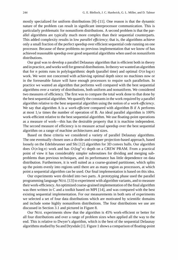
The MPI and C implementation uses our basic algorithm as a coarse-grained parti-tioner to break the problem into one region per processor. Our experiments show thatthis approach achieves good speedup on a range of architectures, including the IBMSP2, Cray T3D, SGI Power Challenge, and DEC AlphaCluster. As an example, Figure 2shows running times for up to 64 processors on the Cray T3D (see Section 3.3 for fullresults). We note that the implementation not only gives speedups that are within a fac-tor of 2 of optimal (compared with a good sequential algorithm), but allow us to solvemuch larger problems because of the additional memory that is available across multipleprocessors. Our algorithm never requires that all the data reside on one processor—boththe input and output are evenly distributed across the processors, as are all intermediateresults.
1.1. Background and Choices.
Theoretical Algorithms. Many of the efficient algorithms for Delaunay triangulation,sequential and parallel, are based on the divide-and-conquer paradigm. These algorithmscan be characterized by the relative costs of the divide and merge phases. An earlysequential approach, developed for Voronoi diagrams by Shamos and Hoey [15] andrefined for Delaunay triangulation by Guibas and Stolfi [16], is to divide the point setinto two subproblems using a median, then to find the Delaunay diagram of each half,and finally to merge the two diagrams. The merge phase does most of the work ofthe algorithm and runs inO(n) time, so the whole algorithm runs inO(n logn) time.Unfortunately, these original versions of the merge were highly sequential in nature.Aggarwal et al. [3] first presented a parallel version of the merge phase, which lead
246 G. E. Blelloch, J. C. Hardwick, G. L. Miller, and D. Talmor
Fig. 2. Scalability of the MPI and C implementation of our algorithm on the Cray T3D, showing the time totriangulate 16k–128k points per processor for a range of machine sizes. For clarity, only the fastest (uniform)and slowest (line) distributions are shown.
to an algorithm withO(log2 n) depth. However, this algorithm was significantly morecomplicated than the sequential version, and was not work-efficient—the merge requiredO(n logn) work. Cole et al. [4] improved the method and made it work-efficient on theCREW PRAM using the same depth. The algorithm, however, remains hampered bymessy data structures, and as it stands can be ruled out as a promising candidate forimplementation. We note, however, that there certainly could be simplifications thatmake it easier to implement.
Reif and Sen [6] developed a randomized parallel divide-and-conquer paradigm,called “polling.” They solve the more general 3D convex hull problem, which can beused for finding the Delaunay triangulation. The algorithm uses a sample of the points toto split the problem into a set of smaller independent subproblems. The size of the sampleensures even splitting with high probability. The work of the algorithm is concentratedin the divide phase, and merging simply glues the solutions together. Since a point canappear in more than one subproblem, trimming techniques are used to avoid blow-up. Asimplified version of this algorithm was considered by Su [11]. He showed that whereassampling does indeed evenly divide the problem, the expansion factor is close to 6 onall the distributions he considered. This will lead to an algorithm that is at best one-sixthwork-efficient, and therefore, pending further improvements, is not a likely candidate forimplementation. Dehne et al. [17] derive a similar algorithm based on sampling. Theyshow that the algorithm is communication-efficient whenn > p3+ε (only O(n/p) datais sent and received by each processor). The algorithm is quite complicated, however,and it is unclear what the constants in the work are.
Edelsbrunner and Shi [12] present a 3D convex hull algorithm based on the 2Dalgorithm of Kirkpatrick and Seidel [18]. The algorithm divides the problem by first usinglinear programming to find a facet of the 3D convex hull above a splitting point, then usingprojection onto vertical planes and 2D convex hulls to find two paths of convex hull edges.These paths are then used to divide the problem into four subproblems, using planar pointlocation to decide for each point which of the subproblems it belongs to. The merge phaseagain simply glues the solutions together. The algorithm takesO(n log2 h) time, whereh

Design and Implementation of a Practical Parallel Delaunay Algorithm 247
is the number of facets in the solution. When applied to Delaunay triangulation, however,the algorithm takesO(n log2 n) time since the number of facets will be2(n). Thisalgorithm can be parallelized without much difficulty since all the substeps have knownparallel solutions, giving a depth (parallel time) ofO(log3 n) and work ofO(n log2 h).Ghouse and Goodrich [7] showed how the algorithm could be improved toO(log2 n)depth andO(min(n log2 h,n logn)) work using randomization and various additionaltechniques. The improvement in work makes the algorithm asymptotically work-efficientfor Delaunay triangulation. However, these work bounds were based on switching to theReif and Sen algorithm if the output size was large. Therefore, when used for Delaunaytriangulation, the Ghouse and Goodrich algorithm simply reduces to the Reif and Senalgorithm.
Implementations. Most of the parallel implementations of Delaunay triangulation usedecomposition techniques such as bucketing [8]–[11] or striping [19]. These techniqueshave the advantage that they can reduce communication by allowing the algorithm topartition points quickly into one bucket (or stripe) per processor and then use sequentialtechniques within the bucket. However, the algorithms rely on the input dataset having auniform spatial distribution of points in order to avoid load imbalances between proces-sors. Their performance on nonuniform distributions more characteristic of real-worldproblems can be significantly worse than on uniform distributions. For example, the 3Dalgorithm by Teng et al. [10] was up to five times slower on nonuniform distributionsthan on uniform ones (on a 32-processor CM-5), while the 3D algorithm by Cignoni etal. [9] was up to ten times slower on nonuniform distributions than on uniform ones (ona 128-processor nCUBE).
Even given the limitation to uniform distributions, the speedups of these algorithmsover efficient sequential code has not been good. Of the algorithms that quote suchspeedups the 2D algorithm by Su [11] achieved speedup factors of 3.5–5.5 on a 32-processor KSR-1, for a parallel efficiency of 11–17%, while the 3D algorithm by Mer-riam [8] achieved speedup factors of 6–20 on a 128-processor Intel Gamma, for a parallelefficiency of 5–16%. Both of these results were for uniform distributions. The 2D al-gorithm by Chew et al. [20], which can handle nonuniform distributions and solves themore general problem of constrained Delaunay triangulation in a meshing algorithm,achieves speedup factors of 3 on an 8-processor SP2, for a parallel efficiency of 38%.However, this algorithm currently requires that the boundaries between processors becreated by hand.
1.2. Our Algorithm and Experiments. Previous results do not look promising for de-veloping practical Delaunay triangulation codes. The theoretical algorithms seem im-practical because they are complex and have large constants, and the implementationsare either specialized to uniform distributions or require partitioning by hand. We there-fore developed a new algorithm loosely based on the Edelsbrunner and Shi approach.The complicated subroutines in the Edelsbrunner and Shi approach, and the fact thatit requiresO(n log2 n) work when applied to Delaunay triangulation, initially seems torule it out as a reasonable candidate for parallel implementation. We note, however, thatby restricting ourselves to a point set on the surface of a sphere or parabola (sufficient forDelaunay triangulation) the algorithm can be greatly simplified. Under this assumption,
248 G. E. Blelloch, J. C. Hardwick, G. L. Miller, and D. Talmor
we developed an algorithm that only needs a 2D convex hull as a subroutine, removingthe need for linear programming and planar point location. Furthermore, our algorithmonly makes cuts parallel to thex or y axis, allowing us to keep the points sorted anduse anO(n) work 2D convex hull. These improvements reduce the theoretical work toO(n logn) and also greatly reduce the constants. This simplified version of the Edels-brunner and Shi approach seemed a promising candidate for experimentation: it doesnot suffer from unnecessary duplication, as points are duplicated only when a Delaunayedge is found, and it does not require complicated subroutines, especially if one is will-ing to compromise by using components that are not theoretically optimal, as discussedbelow.
We initially prototyped the algorithm in the programming language NESL[13], a highlevel parallel programming language designed for algorithm specification and teaching.NESL allowed us to develop the code quickly, try several variants of the algorithm,and run many experiments to analyze the characteristics. For such prototyping NESL
has the important properties that it is deterministic, uses simple parallel constructs, hasimplicit memory management with garbage collection and full bounds checking, andhas an integrated interactive environment with visualization tools. We refined the initialalgorithm through alternating rounds of experimentation and algorithmic design. Weimprove the basic algorithm from a practical point of view by using the 2D convex hullalgorithm of Chan et al. [21]. This algorithm has nonoptimal theoretical work sinceit runs in worst caseO(n logh) work instead of linear (for sorted input). However, inpractice our experiments show that it runs in linear work, and has a smaller constant thanthe provably linear work algorithm. Our final algorithm is not only simple enough tobe easily implemented, but is also highly parallel and performs work comparable withefficient sequential algorithms over a wide range of distributions. We also observed thatthe algorithm can be used effectively to partition the problem into regions in which thework on each region is approximately equal.
After running the experiments in NESL and settling on the specifics of an algorithmwe implemented it in C and MPI [14] with the aid of the Machiavelli toolkit [22]. Thisimplementation uses our algorithm as a coarse-grained partitioner, as outlined above,and then uses a sequential algorithm to finish the subproblems. Although in theory acompiler could convert the NESL code into efficient C and MPI code, significantly moreresearch is necessary to get the compiler to that stage.
Section 2 describes the algorithm and its implementation in NESL, and its translationinto MPI and C. Section 3 describes the experiments we ran on the two implementations.
2. Projection-Based Delaunay Triangulation. In this section we first present ouralgorithm, concentrating on the theoretical motivations for our design choices, thendiscuss particular choices made in the NESL implementation, and finally discuss choicesmade in the C and MPI implementation.
The basic algorithm uses a divide-and-conquer strategy. Figure 3 gives a pseudocodedescription of the algorithm. Each subproblem is determined by a regionR which is theunion of a collection of Delaunay triangles. The regionR is represented by the followinginformation: (1) the polygonal borderB of the region, composed of Delaunay edges,
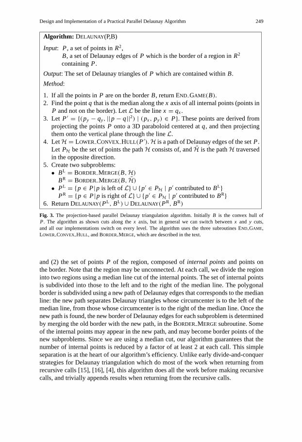
Design and Implementation of a Practical Parallel Delaunay Algorithm 249
Algorithm: DELAUNAY (P,B)
Input: P, a set of points inR2,B, a set of Delaunay edges ofP which is the border of a region inR2
containingP.
Output: The set of Delaunay triangles ofP which are contained withinB.
Method:
1. If all the points inP are on the borderB, return END GAME(B).2. Find the pointq that is the median along thex axis of all internal points (points in
P and not on the border). LetL be the linex = qx.3. Let P′ = {(py − qy, ||p− q||2) | (px, py) ∈ P}. These points are derived from
projecting the pointsP onto a 3D paraboloid centered atq, and then projectingthem onto the vertical plane through the lineL.
4. LetH = LOWER CONVEX HULL(P′).H is a path of Delaunay edges of the setP.Let PH be the set of points the pathH consists of, andH is the pathH traversedin the opposite direction.
5. Create two subproblems:• BL = BORDER MERGE(B,H)
BR = BORDER MERGE(B, H)• PL = {p ∈ P|p is left ofL} ∪ {p′ ∈ PH | p′ contributed toBL}
PR = {p ∈ P|p is right ofL} ∪ {p′ ∈ PH | p′ contributed toBR}6. Return DELAUNAY (PL, BL) ∪ DELAUNAY (PR, BR)
Fig. 3. The projection-based parallel Delaunay triangulation algorithm. InitiallyB is the convex hull ofP. The algorithm as shown cuts along thex axis, but in general we can switch betweenx and y cuts,and all our implementations switch on every level. The algorithm uses the three subroutines END GAME,LOWER CONVEX HULL, and BORDER MERGE, which are described in the text.
and (2) the set of pointsP of the region, composed ofinternal pointsand points onthe border. Note that the region may be unconnected. At each call, we divide the regioninto two regions using a median line cut of the internal points. The set of internal pointsis subdivided into those to the left and to the right of the median line. The polygonalborder is subdivided using a new path of Delaunay edges that corresponds to the medianline: the new path separates Delaunay triangles whose circumcenter is to the left of themedian line, from those whose circumcenter is to the right of the median line. Once thenew path is found, the new border of Delaunay edges for each subproblem is determinedby merging the old border with the new path, in the BORDER MERGEsubroutine. Someof the internal points may appear in the new path, and may become border points of thenew subproblems. Since we are using a median cut, our algorithm guarantees that thenumber of internal points is reduced by a factor of at least 2 at each call. This simpleseparation is at the heart of our algorithm’s efficiency. Unlike early divide-and-conquerstrategies for Delaunay triangulation which do most of the work when returning fromrecursive calls [15], [16], [4], this algorithm does all the work before making recursivecalls, and trivially appends results when returning from the recursive calls.
250 G. E. Blelloch, J. C. Hardwick, G. L. Miller, and D. Talmor
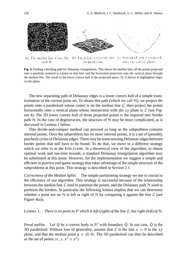
Fig. 4.Finding a dividing path for Delaunay triangulation. This shows the median line, all the points projectedonto a parabola centered at a point on that line, and the horizontal projection onto the vertical plane throughthe median line. The result of the lower convex hull in the projected space,H, is shown in highlighted edgeson the plane.
The new separating path of Delaunay edges is a lower convex hull of a simple trans-formation of the current point set. To obtain this path (which we callH), we project thepoints onto a paraboloid whose center is on the median lineL, then project the pointshorizontally onto a vertical plane whose intersection with thexy plane isL (see Fig-ure 4). The 2D lower convex hull of those projected points is the required new borderpathH. In the case of degeneracies, the structure ofH may be more complicated, as isdiscussed in Lemma 1 below.
This divide-and-conquer method can proceed as long as the subproblem containsinternal points. Once the subproblem has no more internal points, it is a set of (possiblypinched) cycles of Delaunay edges. There may be some missing Delaunay edges betweenborder points that still have to be found. To do that, we move to a different strategywhich we refer to as the END GAME. In a theoretical view of the algorithm, to obtainoptimal work and run-time bounds, a standard Delaunay triangulation algorithm maybe substituted at this point. However, for the implementation we suggest a simple andefficient in practice end-game strategy that takes advantage of the simple structure of thesubproblems at this point. This strategy is described in Section 2.1.
Correctness of the Median Splits. The simple partitioning strategy we use is crucial tothe efficiency of our algorithm. This strategy is successful because of the relationshipbetween the median lineL used to partition the points, and the Delaunay pathH used topartition the borders. In particular the following lemma implies that we can determinewhether a point not onH is left or right ofH by comparing it against the lineL (seeFigure 4(a)).
LEMMA 1. There is no point in P which is left(right) of the lineL, but right(left) ofH.
Proof outline. Let Q be a convex body inR3 with boundaryQ. In our case,Q is the3D paraboloid. Without loss of generality, assume thatL is the linex = 0 in thexyplane, and that the median pointq = (0,0). The 3D paraboloid can then be describedas the set of points(x, y, x2+ y2).
Design and Implementation of a Practical Parallel Delaunay Algorithm 251
A point q in Q is said to belight if it is visible from the x direction, i.e., the ray{q + αx|α > 0} does not intersect the interior ofQ, wherex = (1,0,0). We say thepointq is dark if the ray{q−αx|α > 0} does not intersect the interior ofQ. A point thatis both light and dark is said to be on thesilhouette. The silhouette forms a border betweenlight and dark points. Note that points on thexy plane with a negativex coordinate aremapped using the paraboloid mapping to a dark point.
The set of Delaunay points in the plane,P, is mapped to a set of 3D pointsT onthe paraboloidQ. Let T stand for the convex hull ofT , and letT be the interior solidbounded byT . Clearly,T is a convex body contained inQ. We can classify points onTas dark, light, and silhouette as well.
T is composed of linear faces, edges, and points. For ease of exposition, we assumeno faces appear on the silhouette. We also assume that the points are in general position,i.e., that all faces are triangular.H, the projection of the silhouette ofT on the plane, isthen a simple path.
Note that the pointsT are both onT and on Q. Furthermore, if a point ofT isdark (light) in Q, it is also dark (light) inT . However, if a point is dark inQ, its 2Dprojection is left of or onL. If a point is dark inT , its 2D projection is left of or on thepathH. Therefore if a point is left of or onL, then it is left of or onH. This propertyand hence the statement of the lemma is true in the more general setting in whichQis an arbitrary convex body,L is the projection of its silhouette onto the plane,T isan arbitrary set of points onQ, andH is the projection of the silhouette ofT onto theplane.
We now give a simple characterization of when a face onT is light, dark, or on thesilhouette in term of its circumscribing circle (assumingT lie on the paraboloid).
DEFINITION 1. A Delaunay triangle is called a left, right, or middle triangle with respectto a lineL, if the circumcenter of its Delaunay circle lies left of, right of, or on the lineL, respectively.
LEMMA 2. A face F is strictly dark, strictly light, or on the silhouette if and only if itstriangle in the plane is left, right, or middle, respectively.
PROOF. The supporting plane of faceF is of the formax+ by− z = c with normaln = (a,b,−1). Now F is strictly dark, light, or on the silhouette if and only ifa < 0,a > 0, ora = 0, respectively. The vertical projection of the intersection of this plane, andthe paraboloid, is described byx2+ y2 = ax+by+c, or by(x−a/2)2+ (y−a/2)2 =c+ (a/2)2+ (b/2)2. This is an equation describing a circle whose center is(a/2,b/2)and contains the three points of the triangle. Hence, this is the Delaunay triangle’scircumcenter and this circumcenter is simply related to the normal of the correspondingface of the convex hull.
Therefore the only time that a triangle will cause a face to be on the silhouette is whenits circumcenter is onL. For ease of exposition, we assume the following degeneracycondition: no vertical or horizontal line contains both a point and a circumcenter. Ingeneral we could allow faces on the silhouette in which caseH would could include

252 G. E. Blelloch, J. C. Hardwick, G. L. Miller, and D. Talmor
triangles (or other shapes if degeneracies are allowed so that faces are not triangles).We could then split the path into one that goes around the triangles to the left (HL) andone that goes around the triangles to the right (HR) and use these to merge with the oldborder for the recursive calls.
Analysis. We now consider the total work and depth of the algorithm, basing ouranalysis on a CREW PRAM. The costs depend on the three subroutines END GAME,LOWER CONVEX HULL, and BORDER MERGE. In this section we briefly describe sub-routines that lead to theoretically reasonable bounds, and in the following sections wediscuss variations for which we do not know how to prove strong bounds on, but workbetter on our data sets.
LEMMA 3. Using a parallel version of Overmars and van Leeuwen’s algorithm[23]for theLOWER CONVEX HULL and Cole et al.’s algorithm [4] for theEND GAME, ourmethod runs in O(n logn) work and O(log3 n) depth.
PROOF. We first note that since our projections are always on a plane perpendicular to thex or y axis, we can keep our points sorted relative to these axes with linear work (we cankeep the rank of each point along both axes and compress these ranks when partitioning).This allows us to use Overmars and van Leeuwen’s linear-work algorithm [23] for 2Dconvex hulls on sorted input. Since their algorithm uses divide-and-conquer and eachdivide stage takesO(logn) serial time, the full algorithm runs withO(log2 n) depth. Theother subroutines in the partitioning are the median, projection, and BORDER MERGE.These can all be implemented within the bounds of the convex hull (BORDER MERGEisdiscussed later in this section). The total cost for partitioningn points is thereforeO(n)work andO(log2 n) depth.
As discussed earlier, when partitioning a region(P, B) the number of internal pointswithin each partition is at most half as many as the number of internal points in(P, B).The total number of levels of recursion before there are no more internal points is thereforeat most logn. Furthermore, the total border size when summed across all instances ona given level of recursion is at most 6n. This is because 3n is a limit on the number ofDelaunay edges in the final answer, and each edge can belong to the border of at mosttwo instances (one on each side). Since the work for partitioning a region is linear, thetotal work needed to process each level isO(n) and the total work across the levels isO(n logn). Similarly, the depth isO(log3 n).
This is the cost to reduce the problem to components which have no internal points,just borders. To finish off we need to run the END GAME. If the border is small—ourexperiments indicate that the average size is less than 10—it can be solved by simplertechniques, such as constructing the triangulation incrementally using point insertion. Ifthe border is large, then the Cole et al. algorithm [4] can be used.
Comparison with Edelsbrunner and Shi. Here we explain how our algorithm differsfrom the original algorithm presented by Edelsbrunner and Shi [12]. Our algorithm usesthe same technique of partitioning the problem into subproblems using a path obtained byprojecting the point set and using a 2D convex hull subroutine. However, we partition thepoints and border by finding a median, computing a 2D convex hull of a simple projection
Design and Implementation of a Practical Parallel Delaunay Algorithm 253
of the points, and then using simple local operations for merging the borders. In contrast,since Edelsbrunner and Shi are solving the more general problem of a 3D convex hull,they have to (1) find a 4-partition using two intersecting lines in thexy plane, (2) uselinear programming to find the face of the convex hull above the intersection, (3) computetwo convex hulls of projections of the points, (4) merge the borders, and (5) use pointlocation to determine which points belong to which partition. Each of these steps is morecomplicated than ours, and in the case of step (3) our is asymptotically faster—it runs inlinear rather than thanO(n logn)—leading to an overall faster algorithm.
We can get away with the simpler algorithm since in our projection in 3D, all pointslie on a surface of a parabola. This allows us to find a face of the convex hull easily—wejust use the median point—and to partition the points simply by using a median line. Thisavoids the linear programming and point location steps (steps (2) and (5)). Furthermore,because of our median cut lemma (Lemma 1), our partitions can all be made parallel tothe x or y axis. This both avoids finding a 4-partition (step (1)) and also allows us inlinear time to keep our points sorted along the cut. Using this sorted order we can usea linear work algorithm for the convex hull, as discussed. This is not possible with theEdelsbrunner and Shi algorithms, since it must make cuts in arbitrary directions in orderto get the 4-partition needed to guarantee progress. On the down side, our partition isnot as good as the 4-partition of Edelsbrunner and Shi since it only guarantees that theinternal points are well partitioned—the border could be badly partitioned. This meanswe have to switch algorithms when no internal points remain. However, our experimentsshow that for all our distributions the average size of components when switching isless than 10, and the maximum size is rarely more than 50 (this assumes that we arealternating betweenx andy cuts).
We note that proving the sufficiency of the median test for the divide phase was theinsight that motivated our choice of the projection-based algorithm for implementation.This work was also motivated by the theoretical algorithms presented in [24].
2.1. NESL Implementation. This section gives more details on the substeps and out-lines the data structures used in the NESL implementation. NESL [13] is a nested data-parallel language that is well suited to expressing irregular divide-and-conquer algo-rithms of this type. It is very high level and allowed us to prototype, debug, and experimentwith variations of the algorithm quickly. The main components of the implementation arethe border merge, the convex hull, and the end game. An important result of our experi-ments was that we noticed that subroutines that are not theoretically optimal sometimeslead to more practical resultes. These subroutines are discussed below.
Border Merge. The border merge consists of merging the new Delaunay path with theold border, to form two new borders. The geometric properties of these paths, combinedwith the data structure we use, lead to a simple and elegantO(n) work, O(1) timeintersection routine.
The set of points is represented using a vector. The borderB is represented as anunordered set of triplets. Each triplet represents a corner of the border, in the form(ia, im, i b), whereim is an index to the middle corner point,ia is an index to the precedingpoint on the border,i b is an index to the following point. Note that the border could havepinch points, i.e.,B could contain two triplets with the same middle point (see Figure 6).

254 G. E. Blelloch, J. C. Hardwick, G. L. Miller, and D. Talmor
Fig. 5.The six cases for merging the new and old border. The old border is in thick lines, and the partitioningpath in dotted lines. The convention in the drawings (and the program) is that the interior lies left of the borderwhen proceeding in the direction of the arrows. The resulting two new borders are in thin lines, with the newleft border marked with double arcs, and the new right border with a single arc.
The 2D convex hull algorithm returns a new border path,H, also represented as a setof triplets.H andB have the following properties:
• No two edges cross since bothB andH are subsets of the set of Delaunay edges ofP.• H is a simple path anchored at its endpoints onB.
The border merge can be computed by considering only the local structure ofH andB. Specifically, we intersect pairs of triplets of equal middle index, one representing theshape of the new border near the point, the other representing the shape of the old border.The existence of pinch points inB does not affect this simple procedure, as each tripletbelonging to the pinched corner can be intersected independently with the new border.Since the new border has distinctim’s the number of corner intersections computed is atmost the number of corners in the old border.
Figure 5 shows the six different cases for the intersection of the old and new triplets.The core of the border merge is therefore a routine receiving two triplets, identifyingwhich of the six cases they fall into, and returning a set of new left border triplets andright border triplets.
2D Convex Hull. The 2D convex hull is central to our algorithm, and is the mostexpensive component. We considered three candidates for the convex hull algorithm:(1) Overmars and van Leeuwens’ [23], which isO(n) work for sorted points. (2) Kirk-patrick and Seidel’sO(n logh) algorithm [18], and its much simplified form as presentedby Chan et al. [21]. (3) A simple worst caseO(n2) quickhull algorithm, as in [25] and[26]. All of these algorithms can be naturally parallelized.
Using the algorithm of Overmars and van Leeuwen [23] the convex hull of presortedpoints can be computed in serialO(n)work, and the parallel extension is straightforward.Since we can presort the point set, and maintain the ordering through thex andy cutswe perform, using Overmars and van Leeuwen’s algorithm will result in linear work foreach convex hull invocation.
With the other algorithms we do not make use of the sorted order. The lower bound forfinding a 2D convex hull for unsorted input isO(n logh) work [18] making it seem that
Design and Implementation of a Practical Parallel Delaunay Algorithm 255
these algorithms should not perform as well given that our output sizesh are typicallyaround
√n. The lower bound, however, is based on pathological distributions in which all
the points are very close to the boundary of the final hull. For more common distributions,such as the ones that appeared in our experiments even with the highly nonuniform input,the algorithms run in what appears to be linear work. This is because the Kirpatrick–Seidel, Chan, and quickhull algorithms all throw away most of the interior points in thefirst few levels of recursion.
Preliminary experiments showed that quickhull outperformed the Overmars and vanLeeuwen algorithm. The experiments also showed, however, that for quickhull someof our distributions resulted in much more costly convex hull phases than the others,in that they seemed to have much higher constants (they still scaled linearly with theinput size). Quickhull advances by using the furthest point heuristic, and, for extremelyskewed distributions, the furthest point does not always provide a balanced split. TheKirpatrick–Seidel and Chan algorithms guarantee good splits but finding the splits ismore expensive making these algorithms slower for the more uniform distributions. Wetherefore use an algorithm that combines a randomized version of Chan et al.’s algorithmwith the quickhull algorithm. Running the quickhull for a few levels makes quick progresswhen possible and prunes out a large fraction of the points. Switching to the Chan et al.algorithm at lower levels guarantees balanced cuts, which might be necessary for pointsets that did not yield to quickhull.
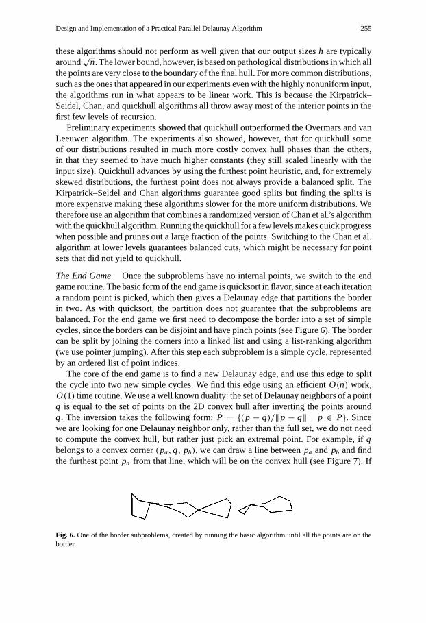
The End Game. Once the subproblems have no internal points, we switch to the endgame routine. The basic form of the end game is quicksort in flavor, since at each iterationa random point is picked, which then gives a Delaunay edge that partitions the borderin two. As with quicksort, the partition does not guarantee that the subproblems arebalanced. For the end game we first need to decompose the border into a set of simplecycles, since the borders can be disjoint and have pinch points (see Figure 6). The bordercan be split by joining the corners into a linked list and using a list-ranking algorithm(we use pointer jumping). After this step each subproblem is a simple cycle, representedby an ordered list of point indices.
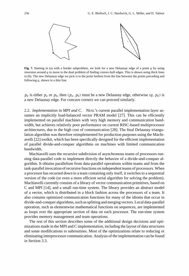
The core of the end game is to find a new Delaunay edge, and use this edge to splitthe cycle into two new simple cycles. We find this edge using an efficientO(n) work,O(1) time routine. We use a well known duality: the set of Delaunay neighbors of a pointq is equal to the set of points on the 2D convex hull after inverting the points aroundq. The inversion takes the following form:P = {(p − q)/‖p − q‖ | p ∈ P}. Sincewe are looking for one Delaunay neighbor only, rather than the full set, we do not needto compute the convex hull, but rather just pick an extremal point. For example, ifqbelongs to a convex corner(pa,q, pb), we can draw a line betweenpa and pb and findthe furthest pointpd from that line, which will be on the convex hull (see Figure 7). If
Fig. 6. One of the border subproblems, created by running the basic algorithm until all the points are on theborder.
256 G. E. Blelloch, J. C. Hardwick, G. L. Miller, and D. Talmor
Fig. 7. Starting in (a) with a border subproblem, we look for a new Delaunay edge of a pointq by usinginversion aroundq to move to the dual problem of finding convex-hull edges. This is shown using thick linesin (b). The new Delaunay edge we pick is to the point farthest from the line between the points preceding andfollowing q, shown in a thin line.
pd is eitherpa or pb, then(pa, pb) must be a new Delaunay edge, otherwise(q, pd) isa new Delaunay edge. For concave corners we can proceed similarly.
2.2. Implementation in MPI and C. NESL’s current parallel implementation layer as-sumes an implicitly load-balanced vector PRAM model [27]. This can be efficientlyimplemented on parallel machines with very high memory and communication band-width, but achieves relatively poor performance on current RISC-based multiprocessorarchitectures, due to the high cost of communication [28]. The final Delaunay triangu-lation algorithm was therefore reimplemented for production purposes using the Machi-avelli [22] toolkit, which has been specifically designed for the efficient implementationof parallel divide-and-conquer algorithms on machines with limited communicationbandwidth.
Machiavelli uses the recursive subdivision of asynchronous teams of processors run-ning data-parallel code to implement directly the behavior of a divide-and-conquer al-gorithm. It obtains parallelism from data-parallel operations within teams and from thetask-parallel invocation of recursive functions on independent teams of processors. Whena processor has recursed down to a team containing only itself, it switches to a sequentialversion of the code (or even a more efficient serial algorithm for solving the problem).Machiavelli currently consists of a library of vector communication primitives, based onC and MPI [14], and a small run-time system. The library provides an abstract modelof a vector, which is distributed in a block fashion across the processors of a team. Italso contains optimized communication functions for many of the idioms that occur individe-and-conquer algorithms, such as splitting and merging vectors. Local data-paralleloperation, such as elementwise mathematical functions on sequences, are implementedas loops over the appropriate section of data on each processor. The run-time systemprovides memory management and team operations.
The rest of this section describes some of the additional design decisions and opti-mizations made in the MPI and C implementation, including the layout of data structuresand some modifications to subroutines. Most of the optimizations relate to reducing oreliminating interprocessor communication. Analysis of the implementation can be foundin Section 3.3.
Design and Implementation of a Practical Parallel Delaunay Algorithm 257
Data Structures. As in the NESL implementation, sets of points are represented byvectors, and borders are composed of triplets. However, these triplets are not balancedacross the processors as the point vectors are, but rather are stored on the same processoras their middle point. A vector of indices is used to link the points inP with the tripletsin the bordersB and H . Given these data structures, the operations of finding internalpoints, and projecting the points onto a parabola (see Figure 3), both reduce to simplelocal loops with no interprocessor communication.
Finding the Median. Initially a parallel version of quickmedian [29] was used to findthe median internal point along thex or y axis. Quickmedian redistributes data amongstthe processors on each recursive step, resulting in high communication overhead. Itwas therefore replaced with a median-of-medians algorithm, in which each processorfirst uses a serial quickmedian to compute the median of its local data, then shares thislocal median with the other processors in a collective communication step, and finallycomputes the median of all the local medians. The result is not guaranteed to be theexact median, but in practice it is sufficiently good for load-balancing purposes; thismodification decreased the running time of the Delaunay triangulation program for thedistributions and machine sizes studied (see Section 3.3) by 4–30%.
Finding the Lower Convex Hull. As in the original algorithm, the pruning variant ofquickhull by Chan et al. [21] is used to find the convex hull. This algorithm tests the slopebetween pairs of points and uses pruning to guarantee that recursive calls have at mostthree-quarters of the original points. However, pairing alln points and finding the medianof their slopes is a significant addition to the basic cost of quickhull. Experimentally,pairing only
√n points was found to be a good compromise between robustness and
performance when used as a substep of Delaunay triangulation (see Section 3.3 foran analysis). As with the median-of-medians approach, the global effects of receivingapproximate results from a subroutine are more than offset by the decrease in runningtime of the subroutine.
Combining Results. The quickhull algorithm concatenates the results of two recursivecalls before returning. In Machiavelli this corresponds to merging two teams of processorsand redistributing their results to form a new vector. However, since this is the lastoperation that the function performs, the intermediate appends in the parallel call tree(and their associated interprocessor communication phases) can be optimized away. Theyare replaced with a single Machiavelli function call at the top of the tree that redistributesthe local result on each processor into a parallel vector shared by all the processors.
Creating the Subproblems. To eliminate an interprocessor communication phase in theborder merge step, the two outer points in a triplet are replicated in the triplet structure,rather than being represented by pointers to point structures (which might well be storedon different processors). All the information required for the line orientation tests canthus be found on the local processor. The memory cost of this replication is analyzed inSection 3.3. Additionally, although Figure 3 shows two calls to the border merge function(one for each direction of the new dividing path), in practice it is faster to make a singlepass, creating both new borders and point sets at the same time.

258 G. E. Blelloch, J. C. Hardwick, G. L. Miller, and D. Talmor
End Game. Since we are using the parallel algorithm as a coarse partitioner, the endgame is replaced with a standard serial Delaunay triangulation algorithm. We chose to usethe version of Dwyer’s algorithm that is implemented in the Triangle mesh generationpackage by Shewchuk [30]. Triangle has a performance comparable with that of theoriginal code by Dwyer, and in addition uses adaptive arithmetic, which is important foravoiding degenerate conditions in nonuniform distributions. Since the input format forTriangle differs from that used by the parallel program, conversion steps are necessarybefore and after calling it. These translate between the pointer-based format of Triangle,which is optimized for sequential code, and the indexed format with triplet replicationused by the parallel code. No changes are necessary to the source code of Triangle.
3. Experiments. In this section we describe the experiments performed on both theNESL and MPI and C implementations. The NESL experiments concentrate on abstractcost measures, and are used to prove the theoretical efficiency of our algorithm. The MPIexperiments concentrate on running time, and are used to prove the practical efficiencyof our production implementation.
3.1. Data Distributions. The design of the data set is always of great importance forthe experimentation and evaluation of an algorithm. Our goal was to test our algo-rithm on distributions that are representative of real-world problems. To highlight theefficiency of our algorithm, we sought to include highly nonuniform distributions thatwould defy standard uniform techniques such as bucketing. We therefore considereddistributions motivated by different domains, such as the distribution of stars in a flatgalaxy (Kuzmin) and point sets originating from mesh generation problems. The densityof our distributions may vary greatly across the domain, but we observed that the result-ing triangulations tend to contain relatively few bad aspect-ratio triangles—especiallywhen contrasted with some artificial distributions, such as points along the diagonalsof a square [1]. Indeed, for the case of uniform distribution, Bern et al. [31] providedbounds on the expected worst aspect ratio. A random distribution with few bad aspect-ratio triangles is advantageous for testing in the typical algorithm design cycle, where itis common to concentrate initially on the efficiency of the algorithm, and only at laterstages concentrate on its robustness. Our chosen distributions are shown in Figure 8 andsummarized here.
• The Kuzmin distribution: this distribution is used by astrophysicists to model thedistribution of star clusters in flat galaxy formations [32]. It is a radially symmetricdistribution whose density falls quickly asr increases, providing a good example ofconvergence to a point. The accumulative probability function as a function of theradiusr is
M(r ) = 1− 1√1+ r 2
.
The point set can be generated by first generatingr , and then uniformly generating apoint on the sphere of radiusr . r itself is generated from the accumulative probabilityfunction by first generating a uniform random variableX, and then equatingr =M−1(X).

Design and Implementation of a Practical Parallel Delaunay Algorithm 259
Fig. 8. Our test-suite of distributions for 1000 points. For the Kuzmin distribution, the figure shows a smallregion in the center of the distribution (otherwise almost all points appear to be at one point at the center).
• Line singularity: this distribution was defined by us as an example of a distributionthat has a convergence area (points very densely distributed along a line segment). Wedefine the probability distribution using a constantb ≥ 0, and a transformation fromthe uniform distribution. Letu andv be two independent, uniform random variablesin the range [0,1], then the transformation is
(x, y) =(
b
u− bu+ b, v
).
In our experiments, we setb = 0.001.• Normal distribution: this consists of points(x, y) such thatx andy are independent
samples from the normal distribution. The normal distribution is also radially sym-metric, but its density at the center is much smaller than in the Kuzmin distribution.• Uniform distribution: this consists of points picked at random in a unit square. It
is important to include a uniform distribution in our experiments for two reasons: tocontrast the behavior of the algorithm over the uniform distribution and the nonuniformdistributions, and also to form common ground for comparison with other relevantwork.
3.2. Experimental Results: NESI. The purpose of these experiments was to measurevarious properties of the algorithm, including the total work (floating-point operations),the parallel depth, the number and sizes of subproblems on each level, and the relativework of the different subroutines. The total work is used to determine how work-efficientthe algorithm is compared with an efficient sequential algorithm, and the ratio of work toparallel depth is used to estimate the parallelism available in the algorithm. We use theother measures to understand better how the algorithm is affected by the distributions, andhow well our heuristic for splitting works. We have also used the measures extensivelyto improve our algorithm and have been able to improve our convex hull by a factor of 3over our initial naive implementation. All these experiments were run using NESL [13]and the measurements were taken by instrumenting the code.
We measured the different quantities over the four distributions, for sizes varyingfrom 210 to 217 points. For each distribution and each size we ran five instances of

260 G. E. Blelloch, J. C. Hardwick, G. L. Miller, and D. Talmor
the distribution (seeded with different random numbers). The results are presented usingmedian values and intervals over these experiments, unless otherwise stated. Our intervalsare defined by the outlying points (the minimum and the maximum over the relevantmeasurements). We defined a floating-point operation as a floating-point comparison orarithmetic operation, though our instrumentation contains a break down of the operationsinto the different classes. The data files are available upon request if a different definitionof work is of interest. Although floating-point operations certainly do not account for allcosts in an algorithm they have the important advantage of being machine independent(at least for machines that implement the standard IEEE floating-point instructions) andseem to have a strong correlation to running time [1], at least for algorithms with similarstructure.
Work. To estimate the work of our algorithm, we compare the floating-point operationcounts with those of Dwyer’s sequential algorithm [33]. Dwyer’s algorithm is a variationof Guibas and Stolfi’s divide-and-conquer algorithm, which is careful about the cuts in thedivide-and-conquer phase so that for quasi-uniform distributions the expected run time isO(n log logn), and on other distributions is at least as efficient as the original algorithm.In a recent paper, Su and Drysdale [1] experimented with a variety of sequential Delaunayalgorithms, and Dwyer’s algorithm performed as well or better than all others across avariety of distributions. It is therefore a good target to compare with. We use the samecode for Dwyer’s algorithm as used in [1]. The results are shown in Figure 1 in theIntroduction.
Our algorithm performance is similar for the line, normal, and uniform distribution,but the Kuzmin distribution is slightly more expensive. To understand the variationamong the distributions, we studied the breakdown of the work into the components ofthe algorithm—finding the median, computing 2D convex hulls, intersecting borders,and the end game. Figure 9 shows the breakdown of floating-point operation counts fora representative example of size 217. These represent the total number of floating-pointoperations used by the components across the full algorithm. As the figure shows, thework for all but the convex hull is approximately the same across distributions (it varies
Fig. 9.Floating-point operation counts partitioned according to the different algorithmic parts, for each distri-bution.
Design and Implementation of a Practical Parallel Delaunay Algorithm 261
Fig. 10.The depth of the algorithm for the different distributions and problem sizes.
by less than 10%). For the convex hull, the Kuzmin distribution requires about 25% morework than the uniform distribution. Our experiments show that this is because after theparaboloid lifting and projection, the convex hull removes fewer points in early stepsand therefore requires more work. In an earlier version of our implementation in whichwe used a simple quickhull instead of the balanced algorithm [21], Kuzmin was 75%more expensive than the others.
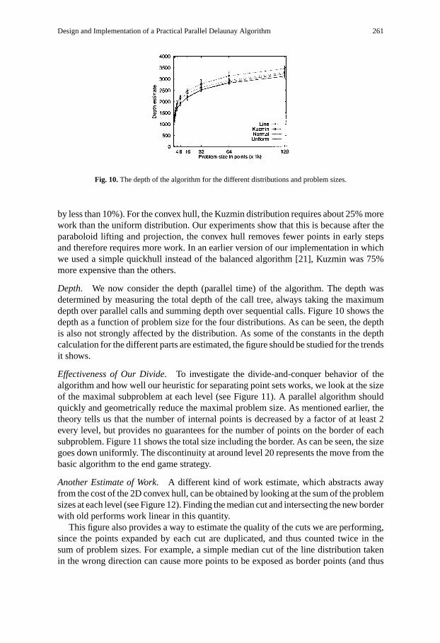
Depth. We now consider the depth (parallel time) of the algorithm. The depth wasdetermined by measuring the total depth of the call tree, always taking the maximumdepth over parallel calls and summing depth over sequential calls. Figure 10 shows thedepth as a function of problem size for the four distributions. As can be seen, the depthis also not strongly affected by the distribution. As some of the constants in the depthcalculation for the different parts are estimated, the figure should be studied for the trendsit shows.
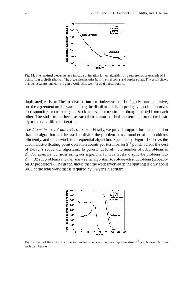
Effectiveness of Our Divide. To investigate the divide-and-conquer behavior of thealgorithm and how well our heuristic for separating point sets works, we look at the sizeof the maximal subproblem at each level (see Figure 11). A parallel algorithm shouldquickly and geometrically reduce the maximal problem size. As mentioned earlier, thetheory tells us that the number of internal points is decreased by a factor of at least 2every level, but provides no guarantees for the number of points on the border of eachsubproblem. Figure 11 shows the total size including the border. As can be seen, the sizegoes down uniformly. The discontinuity at around level 20 represents the move from thebasic algorithm to the end game strategy.
Another Estimate of Work. A different kind of work estimate, which abstracts awayfrom the cost of the 2D convex hull, can be obtained by looking at the sum of the problemsizes at each level (see Figure 12). Finding the median cut and intersecting the new borderwith old performs work linear in this quantity.
This figure also provides a way to estimate the quality of the cuts we are performing,since the points expanded by each cut are duplicated, and thus counted twice in thesum of problem sizes. For example, a simple median cut of the line distribution takenin the wrong direction can cause more points to be exposed as border points (and thus
262 G. E. Blelloch, J. C. Hardwick, G. L. Miller, and D. Talmor
Fig. 11.The maximal piece size as a function of iteration for our algorithm on a representative example of 217
points from each distribution. The piece size includes both internal points and border points. The graph showsthat our separator and our end game work quite well for all the distributions.
duplicated) early on. The line distribution does indeed seem to be slightly more expensive,but the agreement on the work among the distributions is surprisingly good. The curvescorresponding to the end game work are even more similar, though shifted from eachother. The shift occurs because each distribution reached the termination of the basicalgorithm at a different iteration.
The Algorithm as a Coarse Partitioner. Finally, we provide support for the contentionthat the algorithm can be used to divide the problem into a number of subproblemsefficiently, and then switch to a sequential algorithm. Specifically, Figure 13 shows theaccumulative floating-point operation counts per iteration on 217 points versus the costof Dwyer’s sequential algorithm. In general, at leveli the number of subproblems is2i . For example, consider using our algorithm for five levels to split the problem into25 = 32 subproblems and then use a serial algorithm to solve each subproblem (probablyon 32 processors). The graph shows that the work involved in the splitting is only about30% of the total work that is required by Dwyer’s algorithm.
Fig. 12. Sum of the sizes of all the subproblems per iteration, on a representative 217 points example fromeach distribution.

Design and Implementation of a Practical Parallel Delaunay Algorithm 263
Fig. 13.The cumulative work in floating-point operation counts per iteration, for a representative 217 pointsexample from each distribution. The idea is to see how much work it is to divide the problem into 2i problemsin level i , versus the median cost of the sequential algorithm.
3.3. Experimental Results: MPI and C. In this section we present experimental resultsfor the MPI and C implementation on four machines, and analyze where the bottlenecksare, the reasons for any lack of scalability, and the effect of some of the implementationdecisions presented in Section 2.2 on both running time and memory use. Unlike theprevious section which considered work in terms of floating-point operations, this sectionreports running times and therefore includes all other costs such as communication andsynchronization.
To test portability, we used four parallel architectures: a loosely coupled workstationcluster (DEC AlphaCluster) with 8 processors, a shared-memory SGI Power Challengewith 16 processors, a distributed-memory Cray T3D with 64 processors, and a distributed-memory IBM SP2 with 16 processors. To test parallel efficiency, we compared timingswith those on one processor, when the program immediately switches to the sequentialTriangle package [30]. To test the ability to handle nonuniform distributions we used thefour distributions specified earlier. All timings represent the average of five runs usingdifferent seeds for a pseudorandom number generator. For a given problem size and seedthe input data is the same regardless of the architecture and number of processors.
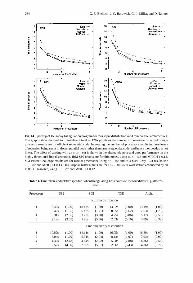
Speedup. To illustrate the algorithm’s parallel efficiency, Figure 14 shows the time totriangulate 217 points on different numbers of processors, for each of the four platformsand the four different distributions. This is the largest number of points that can betriangulated on one processor of all four platforms. Speedup is not perfect because asmore processors are added, more levels of recursion are spent in parallel code ratherthan in the faster sequential code. However, we still achieve approximately 50% parallelefficiency for the distributions and machine sizes tested—that is, we achieve about halfof the perfect speedup over efficient sequential code. Additionally, the Kuzmin and linedistributions show similar speedups to the uniform and normal distributions, confirmingthat the algorithm is effective at handling nonuniform distributions as well as uniformones. Data for the Kuzmin and line singularity distributions are also shown in Table 1.Note that the Cray T3D and the DEC AlphaCluster use the same 150 MHz Alpha 21064processors, and their single-processor times are thus comparable. However, the T3D’s
264 G. E. Blelloch, J. C. Hardwick, G. L. Miller, and D. Talmor
Fig. 14.Speedup of Delaunay triangulation program for four input distributions and four parallel architectures.The graphs show the time to triangulate a total of 128k points as the number of processors is varied. Singleprocessor results are for efficient sequential code. Increasing the number of processors results in more levelsof recursion being spent in slower parallel code rather than faster sequential code, and hence the speedup is notlinear. The effect of starting with anx or y cut is shown in the alternately poor and good performance on thehighly directional line distribution. IBM SP2 results are for thin nodes, usingxlc -O3 and MPICH 1.0.12.SGI Power Challenge results are for R8000 processors, usingcc -O2 and SGI MPI. Cray T3D results usecc -O2 and MPICH 1.0.13. DEC AlphaCluster results are for DEC 3000/500 workstations connected by anFDDI Gigaswitch, usingcc -O2 and MPICH 1.0.12.
Table 1.Time taken, and relative speedup, when triangulating 128k points on the four different platformstested.
Processors SP2 SGI T3D Alpha
Kuzmin distribution
1 8.42s (1.00) 10.48s (1.00) 13.02s (1.00) 13.19s (1.00)2 5.42s (1.55) 6.12s (1.71) 8.05s (1.62) 7.63s (1.73)4 3.31s (2.55) 3.28s (3.20) 4.25s (3.06) 5.17s (2.55)8 2.19s (3.85) 1.96s (5.36) 2.53s (5.16) 3.89s (3.39)
Line singularity distribution
1 10.82s (1.00) 14.11s (1.00) 16.05s (1.00) 16.39s (1.00)2 6.04s (1.79) 6.91s (2.04) 8.13s (1.97) 7.93s (2.07)4 4.36s (2.48) 4.84s (2.92) 5.58s (2.88) 6.36s (2.58)8 2.52s (4.30) 2.56s (5.51) 2.96s (5.43) 4.36s (3.76)
Design and Implementation of a Practical Parallel Delaunay Algorithm 265
Fig. 15.Scalability of Delaunay triangulation program for two input distributions and four parallel architectures.The graphs show the time to triangulate 16k–128k points per processor as the number of processors is varied.For clarity, only the fastest (uniform) and slowest (line) distributions are shown. Machine setups are as inFigure 14.
specialized interconnection network has lower latency and higher bandwidth than thecommodity FDDI network on the AlphaCluster, resulting in better scalability.
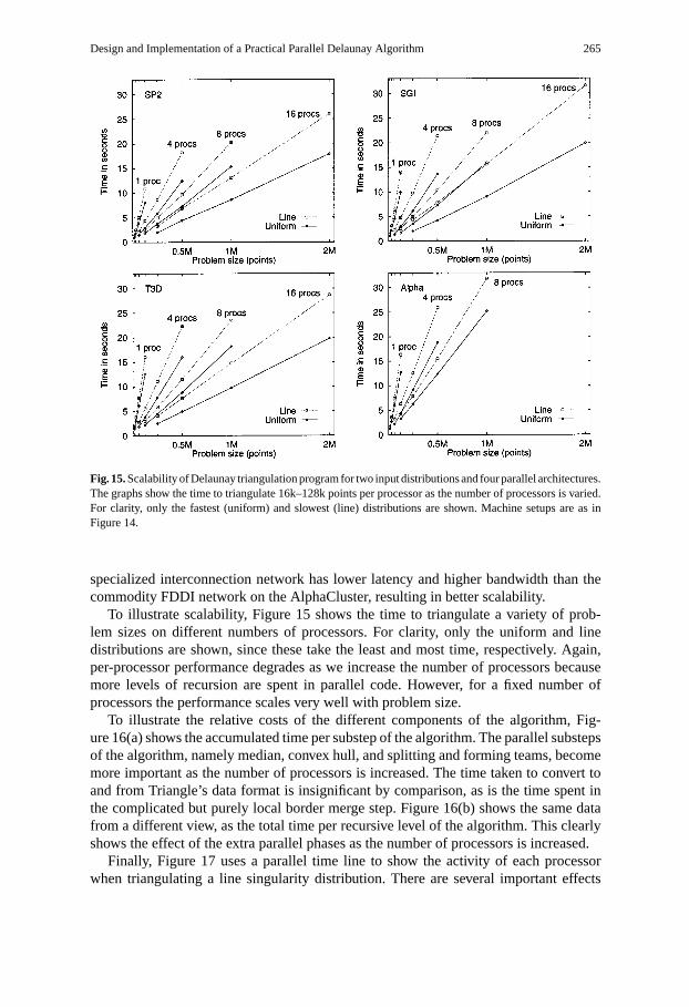
To illustrate scalability, Figure 15 shows the time to triangulate a variety of prob-lem sizes on different numbers of processors. For clarity, only the uniform and linedistributions are shown, since these take the least and most time, respectively. Again,per-processor performance degrades as we increase the number of processors becausemore levels of recursion are spent in parallel code. However, for a fixed number ofprocessors the performance scales very well with problem size.
To illustrate the relative costs of the different components of the algorithm, Fig-ure 16(a) shows the accumulated time per substep of the algorithm. The parallel substepsof the algorithm, namely median, convex hull, and splitting and forming teams, becomemore important as the number of processors is increased. The time taken to convert toand from Triangle’s data format is insignificant by comparison, as is the time spent inthe complicated but purely local border merge step. Figure 16(b) shows the same datafrom a different view, as the total time per recursive level of the algorithm. This clearlyshows the effect of the extra parallel phases as the number of processors is increased.
Finally, Figure 17 uses a parallel time line to show the activity of each processorwhen triangulating a line singularity distribution. There are several important effects

266 G. E. Blelloch, J. C. Hardwick, G. L. Miller, and D. Talmor
Fig. 16. Two views of the execution time as the problem size is scaled with number of processors (IBMSP2, 128k points per processor). (a) The total time spent in each substep of the algorithm. The time spentin sequential code remains approximately constant, while convex hull and team operations (which includessynchronization delays) are the major overheads in the parallel code. (b) The time per recursive level of thealgorithm; note the approximately constant overhead per level.
that can be seen here. First, the nested recursion of the convex hull algorithm within theDelaunay triangulation algorithm. Second, the alternating high and low time spent in theconvex hull, due to the effect of the alternatingx and y cuts on the highly directionalline distribution. Third, the operation of the processor teams. For example, two teams offour processors split into four teams of two just before the 0.94 second mark, and furthersubdivide into eight teams of one processor (and hence switch to sequential code) justafter. Lastly, the amount of time wasted waiting for the slowest processor in the parallelmerge phase at the end of the algorithm is relatively small, despite the very nonuniformdistribution.
Fig. 17. Activity of eight processors over time, showing the parallel and sequential phases of Delaunaytriangulation and its inner convex hull algorithm (IBM SP2, 128k points in a line singularity distribution).A parallel step consists of two phases of Delaunay triangulation code surrounding one or more convex hullphases; this run has three parallel levels. Despite the nonuniform distribution the processors do approximatelythe same amount of sequential work.
Design and Implementation of a Practical Parallel Delaunay Algorithm 267
Memory Requirements. As explained in Section 2.2, border points are replicated intriplet structures to eliminate the need for global communication in the border mergestep. Since one reason for using a parallel computer is to be able to handle larger prob-lems, we would like to know that this replication does not significantly increase thememory requirements of the program. Using 64-bit doubles and 32-bit integers, a pointand associated index vector entry occupies 32 bytes, while a triplet occupies 48 bytes.However, since a border is normally composed of only a small fraction of the total num-ber of points, the additional memory required to hold the replicated triplets is relativelysmall. For example, in a run of 512k points in a line singularity distribution on eightprocessors, the maximum ratio of triplets to total points on a processor (which occursat the switch between parallel and sequential code) is approximately 2000 to 67,000, sothat the triplets occupy less than 5% of required storage. Extreme cases can be manufac-tured by reducing the number of points per processor; for example, with 128k points themaximum ratio is approximately 2000 to 17,500. Even here, however, the triplets stillrepresent less than 15% of required storage, and by reducing the number of points perprocessor we have also reduced absolute memory requirements.
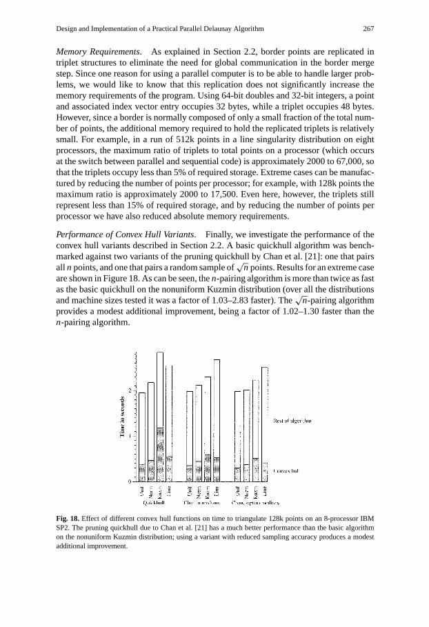
Performance of Convex Hull Variants. Finally, we investigate the performance of theconvex hull variants described in Section 2.2. A basic quickhull algorithm was bench-marked against two variants of the pruning quickhull by Chan et al. [21]: one that pairsall n points, and one that pairs a random sample of
√n points. Results for an extreme case
are shown in Figure 18. As can be seen, then-pairing algorithm is more than twice as fastas the basic quickhull on the nonuniform Kuzmin distribution (over all the distributionsand machine sizes tested it was a factor of 1.03–2.83 faster). The
√n-pairing algorithm
provides a modest additional improvement, being a factor of 1.02–1.30 faster than then-pairing algorithm.
Fig. 18.Effect of different convex hull functions on time to triangulate 128k points on an 8-processor IBMSP2. The pruning quickhull due to Chan et al. [21] has a much better performance than the basic algorithmon the nonuniform Kuzmin distribution; using a variant with reduced sampling accuracy produces a modestadditional improvement.
268 G. E. Blelloch, J. C. Hardwick, G. L. Miller, and D. Talmor
4. Concluding Remarks. In this paper we described an algorithm for Delaunay tri-angulation that is theoretically optimal in work, requires polylogarithmic depth, and isefficient in practice, at least when using some components that are not known to beasymptotically optimal. In particular the main results are:
• The algorithm runs withO(n logn) work andO(log3 n) depth (parallel time) on aCREW PRAM. This is the best bound that we know for a projection-based algorithm(i.e., one that finds the separating path before making recursive calls).• Using a variant of our algorithm that uses nonoptimal subroutines the constants in the
measured work are small enough to be competitive with the best sequential algorithmthat we know of. In particular, depending on the point distribution the algorithm rangesfrom being 40% to 90% work-efficient relative to Dwyer’s algorithm [33].• The algorithm is highly parallel. The ratio of work to parallel time is approximately
104 for 105 points. This gives plenty of freedom on how to parallelize the code andwas crucial in getting good efficiency in our MPI implementation (the additionalparallelism is used to hide message-passing overheads and minimize communication).• An implementation of the algorithm as a coarse partitioner in MPI and C gets bet-
ter speedup than previously reported across a variety of machines and nonuniformdistributions.
References
[1] P. Su and R. Drysdale. A comparison of sequential Delaunay triangulation algorithms.ComputationalGeometry: Theory and Applications, 7:361–386, 1997.
[2] A. Chow. Parallel Algorithms for Geometric Problems. Ph.D. thesis, Department of Computer Science,University of Illinois, Urbana-Champaign, IL, December 1981.
[3] A. Aggarwal, B. Chazelle, L. Guibas, C.O Dunlaing, and C. Yap. Parallel computational geometry.Algorithmica, 3(3):293–327, 1988.
[4] R. Cole, M. T. Goodrich, and C.O Dunlaing. Merging free trees in parallel for efficient Voronoidiagram construction. InProceedings of the17th International Colloquium on Automata, Languagesand Programming, pages 32–45, July 1990.
[5] B. C. Vemuri, R. Varadarajan, and N. Mayya. An efficient expected time parallel algorithm for Voronoiconstruction. InProceedings of the4th Annual ACM Symposium on Parallel Algorithms and Architec-tures, pages 392–400, June 1992.
[6] J. H. Reif and S. Sen. Polling: a new randomized sampling technique for computational geometry. InProceedings of the21st Annual ACM Symposium on Theory of Computing, pages 394–404, May 1989.
[7] M. Ghouse and M.T. Goodrich. In-place techniques for parallel convex hull algorithms. InProceedingsof the3rd Annual ACM Symposium on Parallel Algorithms and Architectures, pages 192–203, July1991.
[8] M. L. Merriam. Parallel implementation of an algorithm for Delaunay triangulation. InProceedings ofthe First European Computational Fluid Dynamics Conference, volume 2, pages 907–912, September1992.
[9] P. Cignoni, D. Laforenza, C. Montani, R. Perego, and R. Scopigno. Evaluation of Parallelization Strate-gies for an Incremental Delaunay Triangulator in E3. Technical Report C93-17, Consiglio Nazionaledelle Ricerche, Rome, November 1993.
[10] Y. A. Teng, F. Sullivan, I. Beichl, and E. Puppo. A data-parallel algorithm for three-dimensional Delaunaytriangulation and its implementation. InProceedings of Supercomputing ’93, pages 112–121. ACM,New York, November 1993.
[11] P. Su. Efficient Parallel Algorithms for Closest Point Problems. Ph.D. thesis, PCS-TR94-238, Depart-ment of Computer Science, Dartmouth College, Hanover, NH, 1994.

Design and Implementation of a Practical Parallel Delaunay Algorithm 269
[12] H. Edelsbrunner and W. Shi. AnO(n log2 h) time algorithm for the three-dimensional convex hullproblem.SIAM Journal on Computing, 20:259–277, 1991.
[13] G. E. Blelloch, S. Chatterjee, J. C. Hardwick, J. Sipelstein, and M. Zagha. Implementation of a portablenested data-parallel language.Journal of Parallel and Distributed Computing, 21(1):4–14, April 1994.
[14] Message Passing Interface Forum. MPI: a message-passing interface standard.International Journal ofSupercomputing Applications and High Performance Computing, 8(3/4):165–419, March–April 1994.
[15] M. I. Shamos and D. Hoey. Closest-point problems. InProceedings of the16th IEEE Annual Symposiumon Foundations of Computer Science, pages 151–162, October 1975.
[16] L. Guibas and J. Stolfi. Primitives for the manipulation of general subdivisions and the computation ofVoronoi diagrams.ACM Transactions on Graphics, 4(2):74–123, 1985.
[17] F. Dehne, X. Deng, P. Dymond, A. Fabri, and A. A. Khokhar. A randomized parallel 3D convex hullalgorithm for coarse grained multicomputers. InProceedings of the7th Annual ACM Symposium onParallel Algorithms and Architectures, pages 27–33, July 1995.
[18] D. G. Kirkpatrick and R. Seidel. The ultimate planar convex hull algorithm?SIAM Journal on Comput-ing, 15(1):287–299, February 1986.
[19] J. R. Davy and P. M. Dew. A note on improving the performance of Delaunay triangulation. InPro-ceedings of Computer Graphics International ’89, pages 209–226. Springer-Verlag, New York, 1989.
[20] L. P. Chew, N. Chrisochoides, and F. Sukup. Parallel constrained Delaunay meshing. InProceedingsof the Joint ASME/ASCE/SES Summer Meeting Special Symposium on Trends in Unstructured MeshGeneration, pages 89–96, June 1997.
[21] T. M. Y. Chan, J. Snoeyink, and C.-K. Yap. Output-sensitive construction of polytopes in four dimensionsand clipped Voronoi diagrams in three. InProceedings of the6th Annual ACM–SIAM Symposium onDiscrete Algorithms, pages 282–291, 1995.
[22] J. C. Hardwick. An efficient implementation of nested data parallelism for irregular divide-and-conqueralgorithms. InProceedings of the First International Workshop on High-Level Programming Modelsand Supportive Environments, pages 105–114. IEEE, New York, April 1996.
[23] M. H. Overmars and J. van Leeuwen. Maintenance of configurations in the plane.Journal of Computerand System Sciences, 23(2):166–204, October 1981.
[24] G. L. Miller, D. Talmor, S.-H. Teng, and N. Walkington. A Delaunay based numerical method for threedimensions: generation, formulation and partition. InProceedings of the27th Annual ACM Symposiumon Theory of Computing, pages 683–692, May 1995.
[25] F. P. Preparata and M. I. Shamos.Computational Geometry—an Introduction. Springer-Verlag, NewYork, 1985.
[26] G. E. Blelloch and J. J. Little. Parallel solutions to geometric problems in the scan model of computation.Journal of Computer and System Sciences, 48(1):90–115, February 1994.
[27] G. E. Blelloch.Vector Models for Data-Parallel Computing. MIT Press, Cambridge, MA, 1990.[28] J. C. Hardwick. Porting a vector library: a comparison of MPI, Paris, CMMD and PVM. InProceedings of
the1994Scalable Parallel Libraries Conference, pages 68–77, October 1994. A longer version appearsas Report CMU-CS-94-200, School of Computer Science, Carnegie Mellon University, Pittsburgh, PA.
[29] C. A. R. Hoare. Algorithm 63 (partition) and algorithm 65 (find).Communications of the ACM, 4(7):321–322, 1961.
[30] J. R. Shewchuk. Triangle: engineering a 2D quality mesh generator and Delaunay triangulator. InM. C. Lin and D. Manocha, editors,Applied Computational Geometry: Towards Geometric Engineering,volume 1148 of Lecture Notes in Computer Science, pages 203–222. Springer-Verlag, Berlin, May 1996.
[31] M. Bern, D. Eppstein, and F. Yao. The expected extremes in a Delaunay triangulation.InternationalJournal of Computational Geometry and Applications, 1(1):79–91, 1991.
[32] A. Toomre. On the distribution of matter within highly flattened galaxies.The Astrophysical Journal,138:385–392, 1963.
[33] R. A. Dwyer. A simple divide-and-conquer algorithm for constructing Delaunay triangulations inO(n log logn) expected time. InProceedings of the2nd Symposium on Computational Geometry,pages 276–284, May 1986.