algorithmic convex geometry - college of computingvempala/acg/notes.pdf · brunn-minkowski...

Algorithmic Convex Geometry

September 2008

Contents

1 Overview 51.1 Learning by random sampling . . . . . . . . . . . . . . . . . . 5

2 The Brunn-Minkowski Inequality 72.1 The inequality . . . . . . . . . . . . . . . . . . . . . . . . . . 8

2.1.1 Proving the Brunn-Minkowski inequality . . . . . . . . 82.2 Grunbaum’s inequality . . . . . . . . . . . . . . . . . . . . . . 10

3 Convex Optimization 153.1 Optimization in Euclidean space . . . . . . . . . . . . . . . . 15

3.1.1 Reducing Optimization to Feasibility . . . . . . . . . . 183.1.2 Feasibility Problem . . . . . . . . . . . . . . . . . . . . 183.1.3 Membership Oracle . . . . . . . . . . . . . . . . . . . . 25

4 Sampling by Random Walks 274.1 Grid Walk . . . . . . . . . . . . . . . . . . . . . . . . . . . . . 28

5 Convergence of Markov Chains 335.1 Example: The ball walk . . . . . . . . . . . . . . . . . . . . . 345.2 Ergodic flow and conductance . . . . . . . . . . . . . . . . . . 35

6 Sampling with the Ball Walk 41

7 The Localization Lemma and an Isoperimetric Inequality 457.0.1 The localization lemma . . . . . . . . . . . . . . . . . 48

3

4 CONTENTS

Chapter 1

Overview

Algorithmic problems in geometry often become tractable with the assump-tion of convexity. Optimization, volume computation, geometric learningand finding the centroid are all examples of problems which are significantlyeasier for convex sets.

We will study this phenomenon in depth, pursuing three tracks thatare closely connected to each other. The first is the theory of geometricinequalities. We begin with classical topics such as the Brunn-Minkowskiinequality, and later deal with more recent developments such as isoperimet-ric theorems for convex bodies and their extensions to logconcave functions.The second track is motivated by the problem of sampling a geometric dis-tribution by a random walk. Here we will develop some general tools anduse them to analyze geometric random walks. The inequalities of the firsttrack play a key role in bounding the rate of convergence of these walks.The last track is the connection between sampling and various algorithmicproblems, most notably, that of computing the volume of a convex body (ormore generally, integrating a logconcave function). Somewhat surprisingly,random sampling will be a common and essential feature of polynomial-timealgorithms for these problems. In some cases, including the volume problem,sampling by a random walk is the only known way to get a polynomial-timealgorithm.

1.1 Learning by random sampling

We will now see our first example of reducing an algorithmic problem to arandom sampling problem. In a typical learning problem, we are presentedwith samples X1, X2, ... from the domain of the function, and have to guess

5

6 CHAPTER 1. OVERVIEW

the values f(Xi). After after each guess we are told whether it was rightor wrong. The objective is to minimize the number of wrong guesses. Oneassumes there is an unknown function f belonging to some known restrictedclass of functions.

As a concrete example, suppose there is a fixed unknown vector ~a ∈ Rn,and our function f is defined by

f(~x) =

True if ~a · ~x ≥ 0False if ~a · ~x < 0

Assume the right answer has components ai ∈ −2b, ..., 2b ⊂ Z. Considerthe following algorithm. At each iteration, choose a random ~a from thosethat have made no mistakes so far, and use that to make the next guess.

If, on every step, we pick the answer according the majority vote of those~a which have made no mistake so far, then every mistake would cut downthe field of remaining voters by at least a factor of 2. As there are 2b(n+1)

voters at the outset, you would make at most (b + 1)n mistakes.

Exercise 1. Show that for the randomized algorithm above,

E(number of mistakes) ≤ 2(b + 1)n.

Chapter 2

The Brunn-MinkowskiInequality

In this lecture, we will prove a fundamental geometric inequality – theBrunn-Minkowski inequality. This inequality relates the volumes of convexsets in high-dimensional spaces. Let us first recall the definition of convexity.

Definition 1. Let K ⊆ Rn. K is a convex set if for any two points x, y ∈ K,and any 0 ≤ λ ≤ 1, λx + (1− λ)y ∈ K.

To motivate the inequality, consider the following version of cutting a(convex) cake: you pick a point x on the cake, your brother makes a singleknife cut and you get the piece that contains x. A natural choice for x isthe centroid. For a convex set K, it is

x =1

Vol(K)

∫y∈K

y dy.

What is the minimum fraction of the cake that you are guaranteed to get?For convenience, let K be a convex body whose centroid is the origin.

Let u ∈ Rn be the normal vector defining the following halfspaces:

H1 = v ∈ Rn : u · v ≥ 0H2 = v ∈ Rn : u · v < 0

Now we can consider the two portions that u cuts out of K:

K1 = H1 ∩K

K2 = H2 ∩K

7

8 CHAPTER 2. THE BRUNN-MINKOWSKI INEQUALITY

We would like to compare Vol(K1) and Vol(K2) with Vol(K).Consider first one dimension – a convex body in one dimension is just a

segment on the real number line. It’s clear that any cut through the centroidof the segment (i.e. the center) divides the area of the segment into two sidesof exactly half the area of the segment.

For two dimensions, this is already a non-trivial problem. Let’s consideran isosceles triangle, whose side of unique length is perpendicular to the xaxis. If we make a cut through the centroid perpendicular to the x axis, itis readily checked that the volume of the smaller side is 4

9 ’ths of the totalvolume. Is this the least possible in R2? What about in Rn?

The Brunn-Minkowski inequality will be very useful in answering thesequestions.

2.1 The inequality

We first define the Minkowski sum of two sets:

Definition 2. Let A,B ⊆ Rn. The Minkowski sum of A and B is the set

A + B = x + y : x ∈ A, y ∈ B

How is the volume of A + B related to the volume of A or B? TheBrunn-Minkowski inequality relates these quantities.

Theorem 3 (Brunn-Minkowski). Let 0 ≤ λ ≤ 1, and suppose that A,B,andλA + (1− λ)B are measurable subsets of Rn. Then,

Vol(λA + (1− λ)B)1/n ≥ λVol(A)1/n + (1− λ)Vol(B)1/n.

Recall that for a measurable set A and a scaling factor λ, we have that:

Vol(λ(A)) = λnVol(A).

It follows that an equivalent statement of the inequality is the following: formeasurable sets A,B and A + B over Rn:

Vol(A + B)1/n ≥ Vol(A)1/n + Vol(B)1/n.

2.1.1 Proving the Brunn-Minkowski inequality

For some intuition, let’s first consider the Brunn-Minkowski inequality whenA and B are axis-aligned cuboids in Rn. A cuboid in Rn is a generalization

2.1. THE INEQUALITY 9

of the familiar rectangle in two dimensions. An axis-aligned cuboid withside lengths (a1, a2, . . . an) is the set

A = x ∈ Rn : li ≤ xi ≤ li + ai

for l = (l1, . . . , ln) ∈ Rn.

Cuboids

Let A be a cuboid with side lengths (a1, a2, . . . , an) and B be a cuboid withside lengths (b1, b2, . . . , bn). Let us prove the Brunn-Minkowski inequalityfor A and B.

This proof will follow easily because if A and B are cuboids, then A+Bis a cuboid with side lengths (a1 + b1, a2 + b2, . . . an + bn). Since these arecuboids, it is easy to compute their volumes:

Vol(A) =n∏

i=1

ai,Vol(B) =n∏

i=1

bi,Vol(A + B) =n∏

i=1

ai + bi

We want to show that

Vol(A + B)1/n ≥ Vol(A)1/n + Vol(B)1/n.

To this end, consider the ratio between the volumes

Vol(A)1/n + Vol(B)1/n

Vol(A + B)1/n=

(∏n

i=1 ai)1/n + (

∏ni=1 bi)

1/n

(∏n

i=1 ai + bi)1/n

=

(n∏

i=1

ai

ai + bi

)1/n

+

(n∏

i=1

bi

ai + bi

)1/n

≤n∑

i=1

ai

ai + bi+

n∑i=1

bi

ai + bi

= 1

Which proves our claim; the inequality used is the standard inequality be-tween the geometric and the arithmetic mean.

Now that we have the result for cuboids, how can we generalize thisto arbitrary measurable sets? The key is that any measurable set can beapproximated arbitrarily well with unions of cuboids. We will prove thatif A ∪ B is the union of a finite number of cuboids, the Brunn-Minkowskiinequality holds. We can prove the general result by approximating arbitrarymeasurable sets with unions of cuboids.


Finite unions of cuboids

We prove the Brunn-Minkowski inequality by induction on the number ofdisjoint cuboids that A∪B contain. Note that our result for A and B beingcuboids is the base case.

We first translate A so that there exists a cuboid in A fully contained inthe halfspace x : x1 ≥ 0 and there exists a cuboid in A fully contained inx : x1 < 0. Now, translate B so that the following inequality holds:

Vol(A+)Vol(A)

=Vol(B+)Vol(B)

where:A+ = A ∩ x : x1 ≥ 0, A− = A \A+

B+ = B ∩ x : x1 ≥ 0, B− = B \B+

Note that we can now proceed by induction on the sets A+ +B+, A−+B−,since the number of cuboids in A+ ∪ B+ and A− ∪ B− is fewer than thenumber of cuboids in A ∪B. This allows us to complete the proof:

Vol(A + B) ≥ Vol(A+ + B+) + Vol(A− + B−)

≥(Vol(A+)1/n + Vol(B+)1/n

)n+(Vol(A−)1/n + Vol(B−)1/n

)n

= Vol(A+)

(1 +

(Vol(B)Vol(A)

)1/n)n

+ Vol(A−)

(1 +

Vol(B)Vol(A)

1/n)n

= Vol(A)

(1 +

(Vol(B)Vol(A)

)1/n)n

It follows that

Vol(A + B)1/n ≥ Vol(A)1/n + Vol(B)1/n

which was our desired result.

2.2 Grunbaum’s inequality

We are now ready to go back to our original question: what is the smallestvolume ratio attainable for the smaller half of a cut through the centroidof any convex body? Somewhat surprisingly, the generalization of the twodimensional case we covered in the introduction is the worst case in highdimensions.

2.2. GRUNBAUM’S INEQUALITY 11

Theorem 4 (Grunbaum’s inequality). Let K be a convex body. Then anyhalf-space defined by a normal vector v that contains the centroid of K con-tains at least a 1

e fraction of the volume of K.

The overview of the proof is that we will consider the body K and ahalfspace defined by v going through the centroid. We will simplify K byperforming a symmetrization step – replacing each (n− 1)-dimensional sliceS of K perpendicular to v with an (n − 1)-dimensional ball of the samevolume as S to obtain a new convex body K ′. We will verify the convexityof K ′ by using the Brunn-Minkowski inequality. This does not modify thefraction of volume contained in the halfspace. Next, we will construct a conefrom K ′. The cone will have the property that the fraction of volume in thehalfspace can only decrease, so it will still be a lower bound on K. Thenwe will easily calculate the ratio of the volume of a halfspace defined by anormal vector v cutting through the centroid of a cone, which will give usthe desired result.

The two steps of symmetrization and conification can be seen in figure2.1.

Figure 2.1: The first diagram shows the symmetrization step – each slice ofK is replaced with an (n− 1) dimensional ball. The second diagram showshow we construct a cone from K ′.

Proof. Assume without loss of generality that v is the x1 axis, and that thecentroid of K is the origin. From the convex body K, we construct a newset K ′. For all α ∈ R, we place an (n− 1) dimensional ball centered aroundc = (α, 0, . . . 0) on the last (n− 1) coordinates with radius rα such that

Vol(B(c, rα)) = Vol(K ∩ x : x1 = α).

See figure 2.1 for a visual of the construction. Recall that the volume of an− 1 dimensional ball of radius r is f(n− 1)rn−1 (where f is a function notdepending on r and only on n), so that we set

rα =(

Vol(K ∩ x : x1 = α)f(n− 1)

)1/(n−1)

We first argue that K ′ is convex. Consider the function r : R → R, definedas r(α) = rα. If r is a concave function (i.e. ∀x, y ∈ R, 0 ≤ λ ≤ 1, r(λx +(1− λ)y) ≥ λr(x) + (1− λ)r(y)), then K ′ is convex.


Note that rα is proportional to Vol(K ∩ x : x1 = α)1/(n−1). LetA = K ∩ x : x1 = a, and let B = K ∩ x : x1 = b. For some 0 ≤ λ ≤ 1,let C = K ∩ x : x1 = λa + (1− λ)b. r is concave if

Vol(C)1/n−1 ≥ λVol(A)1/n−1 + (1− λ)Vol(B)1/n−1 (2.1)

It is easily checked that

C = λA + (1− λ)B

so that (2.1) holds by the Brunn-Minkowski inequality, and K ′ is convex.Let

K ′+ = K ′ ∩ x : x1 ≥ 0

K ′− = K ′ ∩ x : x1 < 0.

Then the ratio of volumes on either side of x1 = 0 has not changed, i.e.

Vol(K ′+) = Vol(K ∩ x : x1 ≥ 0)

Vol(K ′−) = Vol(K ∩ x : x1 < 0).

We argue thatVol(K ′

+)Vol(K ′)

≥ 1e

and the other side will follow by symmetry. To this end, we transform K ′

into a cone (see figure 2.1). To be precise, we replace K ′+ with a cone C of

equal volume with the same base as K ′+. We replace K ′

− with the extensionE of the cone C, such that Vol(E) = Vol(K ′

−). The centroid of K ′ was atthe origin; the centroid of C ∪ E can only be pushed to the right along x1,because r is concave. Let the position of the centroid of C ∪ E along x1 beα ≥ 0. Then we have that

Vol(K ′+)

Vol(K ′)≥ Vol((C ∪ E) ∩ x : x1 ≥ α)

Vol(C ∪ E)

so a lower bound on the latter ratio implies a lower bound onVol(K′

+)

Vol(K′) . Tothis end, we compute the ratio of volume on the right side of a halfspacecutting through the centroid of a cone.

Let the height of the cone C ∪E be h, and the length of the base be R.The centroid of the cone is at position α along x1 given by:

1Vol(C ∪ E)

∫ h

t=0tf(n− 1)

(tR

h

)n−1

dt =f(n− 1)

Vol(C ∪ E)

(R

h

)n−1 ∫ h

t=0tndt

=f(n− 1)

Vol(C ∪ E)· Rn−1h2

n + 1

2.2. GRUNBAUM’S INEQUALITY 13

where f(·) is the function independent of r such that f(n)rn gives the volumeof an n dimensional ball with radius r. By noting that, for a cone,

Vol(C ∪ E) =f(n− 1)Rn−1h

n

we have that α = nn+1h. Now, plugging in to compute the volume of C (the

right half of the cone), we have our desired result.

Vol(C) =∫ n

n+1h

t=0f(n− 1)

(tR

h

)n−1

dt

=Rn−1f(n− 1)

hn−1

∫ nn+1

h

t=0tn−1dt

=(

n

n + 1

)n

Vol(C ∪ E)

≥ 1eVol(C ∪ E)

Chapter 3

Convex Optimization

3.1 Optimization in Euclidean space

Let S ⊂ Rn, and let f : S → R be a real-valued function. The problem ofinterest may be stated as

min f(x)x ∈ S,

(3.1)

that is, find the point x ∈ S which minimizes by f . For convenience, we de-note by x∗ a solution for the problem (3.1) and by f∗ = f(x∗) the associatedcost.

Restricting the set S and the function f to be convex1, we obtain a classof problems which are polynomial-time solvable in

n and log(

1ε

),

where ε defines an optimality criterion such as

‖x− x∗‖ ≤ ε. (3.2)

Linear programming (LP) is one important subclass of this family ofproblems. Let A : Rn → Rm be a linear transformation, b ∈ Rm and c ∈ Rn.We state a LP problem as

minx

cT x

Ax ≥ b.(3.3)

1In fact, one could easily extend to the case of quasi-convex f .

15

16 CHAPTER 3. CONVEX OPTIMIZATION

Here, the feasible set is a polyhedron, for many CO problems it is alsobounded, i.e., it is a polytope.

Here we illustrate other classical examples.

Example 5. Minimum weight perfect matching problem; given graph G =(V,E), with costs ω : E → R, find

min∑

e∈E cexe∑e∈δ(v) xe = 1, for all v ∈ V

xe ∈ 0, 1, for all e ∈ E,

(3.4)

where δ(v) = e = (i, j) ∈ E : v = i or v = j. Due to the last set ofconstraints, the so called integrality constraints, (3.4) is not a LP.

The previous problem had integrality constraints which usually increasethe difficulty of the problem. One possible approach is to solve a linearrelaxation to get (at least) bounds for the original problem. In our particularcase,

min∑

e∈E cexe∑e∈δ(v) xe = 1, for all v ∈ V

0 ≤ xe ≤ 1, for all e ∈ E.

(3.5)

This problem is clearly an LP, and thus, it can be efficiently solved. Un-fortunately, the solution for the LP might not be interesting for the originalproblem (3.4). For example, it is easy to see that the problem (3.4) is infea-sible when |V | = 3, while the linear relaxation is not2.

Surprisingly, it is known that the graph G is bipartite if and only if eachvertex of the polytope defined in (3.5) is a feasible solution for (3.4). Thus,for this particular case, the optimal cost coincide for both problems.

For general graphs, we need to add another family of constraints in orderto obtain the previous equivalence3.∑

e∈(S,Sc)

xe ≥ 1, for all S ⊂ V, |S| odd. (3.6)

Note that there are an exponential number of constraints in this family.Thus, it is not obvious that it is polynomial-time solvable.

Example 6. Another convex optimization problem when a polyhedra is in-tersected with a ball of radius R, i.e., the feasible set is nonlinear.

2Just let x = (0.5, 0.5, 0.5).3The proof is due to Jack Edmonds.

3.1. OPTIMIZATION IN EUCLIDEAN SPACE 17

min cT xAx ≥ b∑n

i=1 x2i ≤ R2.

(3.7)

Example 7. Semi-definite programming (SDP). Here the variable, insteadof being a vector in Rn, is constrained to being a semi-definite positive ma-trix.

min C ·XA ·X ≤ bi, for i = 1, . . . ,mX < 0,

(3.8)

where A · B =∑n

i=1

∑nj=1 AijBij denotes a generalized inner product, and

the last constraints represent

∀y ∈ Rn, yT Xy ≥ 0

which defines an infinite number of linear constraints.

One might notice that it is impossible to explicitly store all constraintsin (3.6) or (7). It turns out that there is an extremely convenient way todescribe the input of a convex programming problem in an implicit way.

Definition 8. A separation oracle for a convex set K ⊂ Rn is an algorithmthat for each x ∈ Rn, either states that x ∈ K, or provides a vector a ∈ Rn

such thataT x < b and aT y ≥ b for all y ∈ K

Exercise Prove that for any convex set, there exists a separation oracle.Returning to our examples,

5. All that is needed is to check each constraint and return a violatedconstraint if it is the case. In the complete formulation, finding aviolating inequality can be done in polynomial time but is nontrivial.

6. A hyperplane tangent to the ball of radius R can be easily constructed.

7. Given X, the separation oracle reduces to finding a vector v such thatXv = −λv for some positive scalar λ. This would imply that

vT Xv = λ ⇒ X · (vvT ) = −λ,

while X · (vvT ) ≥ 0 for all feasible points.


3.1.1 Reducing Optimization to Feasibility

Before proceeding, we will reduce the problem (3.1), under the convexityassumptions previous mentioned, to a feasibility problem. That is, given aconvex set K, find a point on K or prove that K is empty (“give a certificate”that K is empty).

For a scalar parameter t, we define the convex set

K ∩ x ∈ Rn : f(x) ≤ t

If we can find a point in such a convex set, then we can solve (3.1) via binarysearch for the optimal t.

3.1.2 Feasibility Problem

Now, we are going to investigate a convex feasibility algorithm with thefollowing rules:

Input: separate oracle for K, and r, R ∈ R++

(where a ball of radius r contained in K, K is contained in a ball of radius R)Output: A point in K if K is not empty, or give a certificate that K is empty.

Theorem 9. Any algorithm needs n log2Rr oracle calls in the worst case.

Proof. Since we only have access to the oracle, the set K may be in thelargest remaining set at each iteration. In this case, we can reduce the totalvolume at most by 1/2. It may happen for iteration k as long,(

12

)k

<( r

R

)n

which implies that

k < n log2

R

r

In the seminal work of Khachiyan and its extension by GLS, the EllipsoidAlgorithm was proved to require O(n2 log R

r ) iterations for the convex feasi-bility problem. Subsequently, Karmarkar introduced interior points methodsfor the special case of linear programming; the latter turned out to be morepractical (and polynomial-time).

We are going to consider the following algorithm for convex feasibility.


1. P = cube(R), z = 0.2. Call Separation Oracle for z. If z ∈ K stop.3. P := P ∩ x ∈ Rn : aT x ≤ aT z4. Define the new point z ∈ P .5. Repeat steps 2, 3, and 4 N times6. Declare that K is empty.

Two of the steps are not completely defined. It is intuitive that the choiceof the points z will define the number of iterations needed, N . Many choicesare possible here, e.g., the centroid, a random point, the average of randompoints, analytic center, point at maximum distance from the boundary, etc.

For instance, consider the centroid and an arbitrary hyperplane crossingit. As we proved in the previous lecture, P will be divided into two convexbodies, each having at least 1

e of the total volume of the starting set (Grun-baum’s theorem). Since the initial volume is Rn and the final volume is atleast rn, we need at most

log1− 1e

(R

r

)n

= O(

n logR

r

)iterations.

So, we have reduced convex optimization to convex feasibility, and thelatter we reduced to finding centroid. Unfortunately, the problem of findingthe centroid is #P-hard.

Next, let us consider z to be defined as a random point from P . Forsimplicity, consider the case where P is a ball of radius R centered at theorigin. We would like z to be close to the center, so it is of interest toestimate its expected norm.

E[‖x‖] =∫ R

0

Vol(Sn)tn−1

Vol(Bn)Rntdt (3.9)

=n

Rn

∫ R

0tndt =

n

n + 1R. (3.10)

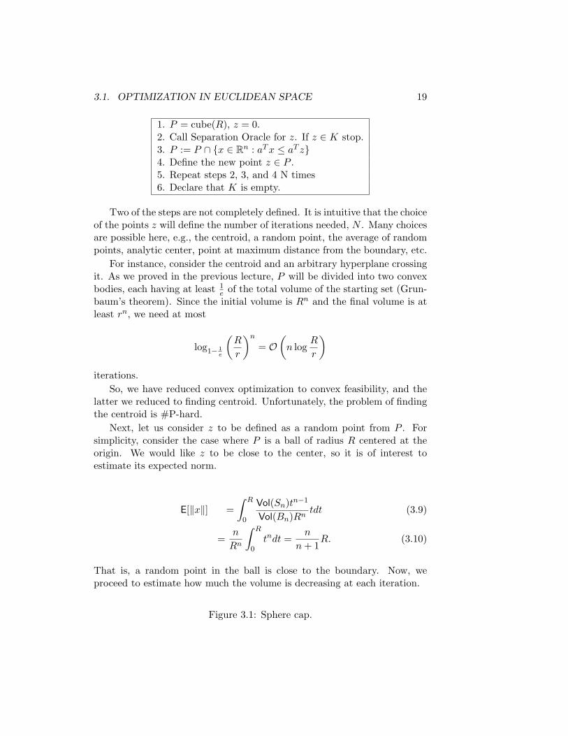
That is, a random point in the ball is close to the boundary. Now, weproceed to estimate how much the volume is decreasing at each iteration.

Figure 3.1: Sphere cap.


Defining b = E[‖x‖] = nn+1R, we obtain a ≤ R

√2

n+1 . This implies thatthe volume is falling by (√

2n + 1

)n

,

which is decreasing exponentially in n. Thus, it will not give us a polynomial-time algorithm.

Now, consider the average of random points,

z =1m

m∑i=1

yi,

where yi’s are i.i.d. points in P .We will prove shortly the following theorem.

Theorem 10. Let z and yimi=1 be defined as above, we have

E[Vol(P ′)] ≤(

1− 1e

+√

n

m

)Vol(P ).

Thus, the following corollary will hold.

Corollary 11. With m = 10n, the algorithm finishes in O(n log Rr ) itera-

tions with high probability.

We will begin to prove Theorem (10) for balls centered at the origin.This implies that E[z] = 0 and, using the radial symmetry,

var(‖z‖) ≤ E[‖z‖2] =1m

E[|yi|2]

=1m

∫ R

0

Vol(Sn)tn−1

Vol(Bn)Rnt2dt

=n

mRn

∫ R

0tn+1dt =

n

m(n + 2)R2.

To conclude the proof for this special case, using the inequality

P

(‖z‖ >

R√n

)≤ V ar(z)n

R2=

nR2

m(n + 2)n

R2≤ n

3m, (3.11)


using m = O(n), with a fixed probability, we obtain ‖z‖ ≤ R√n. Now b = R√

n,

thus,a2 =

(R + R√

n

)(R− R√

n

)= R2

(1− 1

n

). (3.12)

This implies that the volume is falling by(1− 1

n

)n/2

≥ 1√e.

To extend the previous result to an ellipsoid E, it is enough to observethat if A : Rn → Rn is an affine linear transformation, E = AB, whichscales the volume of every subset by the same factor, namely, |det(A)|.

To generalize for arbitrary convex sets, we introduce the following con-cept.

Definition 12. A set S is in isotropic position if for a random point x ∈ S,

1. E[x] = 0;

2. ∀v ∈ Rn, E[(vT x)2] = ‖v‖2.

Next, we are going to prove a lemma which proves an equivalence be-tween the second condition of isotropic position and conditions over thevariance-covariance matrix of the random vector x.

Lemma 13. Let x be a random point in a convex set S, we have ∀v ∈ Rn,E[(vT x)2] = ‖v‖2 if and only if E[xxT ] = I.

Proof. If E[(vT x)2] = ‖v‖2, for v = ei we have

E[(eTi x)2] = E[x2

i ] = 1.

For v := (v1, v2, 0, . . . , 0),

E[(vT x)2] = E[v21x

21 + v2

2x22 + 2v1v2x1x2]

= v21 + v2

2 + 2v1v2E[x1x2]

= v21 + v2

2,

where the last equality follows from the second condition of Definition 12.So, E[x1x2] = 0.

To prove the other direction,

E[(vT x)2] = E[(vT xxT v)] = vT E[xxT ]v = vT v = ‖v‖2.


It is trivial to see that the first condition of isotropic position can beachieved by a translation. It turns out that is possible to obtain the secondcondition by means of a linear transformation.

Lemma 14. Any convex set can be put in isotropic position by an affinetransformation.

Proof. EK [xxT ] = A is positive definite. Then, we can write A = B2 (orBBT ).

Defining, y = B−1x, we get

E[yyT ] = B−1E[xxT ](B−1)T = I.

The new set is defined as

K ′ := B−1(K − z(K)),

where z(K) := E[x], the centroid of K.

Note that the argument used before to relate the proof for balls to ellip-soids states that volume ratios are invariant under affine transformations.Thus, we can restrict ourselves to the case where the convex set is in isotropicposition due to the previous lemma.

Lemma 15. K is a convex body, z is the average of m random points fromK. If H is a half space containing z,

E[Vol(H ∩K)] ≥(

1e−√

n

m

)Vol(K).

Proof. As state before, we can restrict ourselves to the case which K is inisotropic position. Since z = 1

m

∑mi=1 yi,

E[‖z‖2] =1

m2

m∑i=1

E[‖yi‖2] =1m

E[‖yi‖2]

=1m

n∑j=1

E[(yij)

2] =n

m,

where the first equality follows from the independence between yi’s, andequalities of the second line follows from the isotropic position.


Let h be a unit vector normal to H, since the isotropic position is in-variant under rotations, we can assume that h = e1 = (1, 0, . . . , 0).

Define the (n−1)-volume of the slice K∩x ∈ Rn : x1 = y as Voln−1(K∩x ∈ Rn : x1 = y). We can also define the following density function,

fK(y) =Voln−1(K ∩ x ∈ Rn : x1 = y)

Vol(K). (3.13)

Note that this function has the following properties:

1. fK(y) ≥ 0 for all y ∈ R;

2.∫

RfK(y)dy = 1;

3.∫

RyfK(y)dy = 0;

4.∫

Ry2fK(y)dy = 1;

The following technical lemma will give an useful bound to this density(we defer its proof).

Lemma 16. If fK satisfies the previous properties for some convex body K,

maxy

f(y) ≤ n

n + 1

√n

n + 2< 1

Combining this lemma with the bound on the norm of z,

Vol(K ∩ xRn : x1 ≥ z1Vol(K)

=∫ ∞

z1

fK(y)dy

=∫ ∞

0fK(y)dy −

∫ z1

0fK(y)dy

≥ 1e−∫ z1

0max

yfK(y)dy

≥ 1e− ‖z‖

≥ 1e−√

n

m.

(3.14)


Figure 3.2: Construction to increase the moment of inertia I.

Proof. (of Lemma 16) Let K be a convex body in isotropic position forwhich maxy fK(y) is as large as possible. In Figure 3.1.2, we denote byy∗ ∈ arg maxy fK(y), the centroid is zero, and the set K is the black line.

In Figure 3.1.2, the transformation in part I consists of replacing it witha cone whose base is the cross-section at zero and its apex is on the x1 axis.The distance of the apex is defined to preserve the volume of part I. Such atransformation can only move mass to the left of the centroid.

The transformation in part II of figure 3.1.2 is to construct the convexhull between the cross sections at zero and y∗. This procedure may losesome mass (never increases). Part III is also replaced by a cone, with basebeing the cross-section at y∗ and the distance of the apex is such that wemaintain the total volume. Thus, the transformations in parts II and IIImove mass only to the right, i.e., away from the centroid.

Defining the moment of inertia4, as I(K) =∫K(y − EK [y])2fK(y)dy, we

make the following claim.

Claim 17. Moving mass away from the centroid of a set can only increasethe moment of inertia I.

Let us define a transformation C → C ′, x1 → x1+g(x1), where x1g(x1) ≥ 0.

I(C) = V arC(y) = EC [y2]

I(C ′) = V arC′(y) = EC′ [y2]− (EC′ [y])2

= EC [(y + g(y))2]− (EC [y + g(y)])2

= V arC(y) + V arC(g(y)) + 2EC [yg(y)]≥ I(C).

In fact, we have strict inequality if g(y) is nonzero on a set of positivemeasure. In this case, we can shrink the support of fK by a factor strictlysmaller that one, and scale up fK by a factor greater than one to get a setwith moment of inertia equal to 1. In this process max fK has increased.This is a contradiction since we started with maximum possible. Thus, Kmust have the shape of K ′.

Now, we proceed for the transformation in Figure 3.1.2.In Figure 3.1.2, y is chosen to preserve the volume in Part I, while

Part II is not altered. Note that all the mass removed from the segment4Note that EK [y] = 0 since K is in isotropic position.


Figure 3.3: Construction to reduce to a double cone.

between [−y, y] is replaced at a distance to zero greater than y. Thus, themoment of inertia increases. By the same argument used before, we obtaina contradiction. Hence, K must be a double cone.

Once we obtain a double cone, we can move y∗ to the last point to theright, and build a cone with the same volume which has a greater momentof inertia. So K must be this cone with length h and with base area A at

y∗. Then, it is an easy exercise in integration to get h = (n+1)√

n+2n . Since

Vol(K) = Ahn ,

f(y∗) =A

Vol(K)=

n

h=

n

n + 1

√n

n + 2< 1.

3.1.3 Membership Oracle

We have reduced quasi-convex optimization over convex sets to a feasibil-ity problem and solved the latter using a polynomial number of calls to aseparation oracle.

We note that with only a membership oracle, given an arbitrary pointx in the space, it will return a certificate that x ∈ K or a certificate thatx /∈ K, and a point x ∈ K such that x+rB ⊆ K ⊆ x+RB, the optimizationproblem can still be solved using a polynomial number of oracle calls. Theidea is to use the oracle to generate random samples (this part needs only amembership oracle), then restrict the set using the objective function valuesat the sample points. The first polynomial algorithm in this setting wasgiven by GLS using a variant of the Ellipsoid algorithm.

Chapter 4

Sampling by Random Walks

Here we consider the problem of selecting a point uniformly at random froma convex set K. Before attempting a general procedure, let’s consider somespecial cases where we can readily derive sampling procedures.

Cuboid A cuboid is a product of one dimensional intervals, i.e., a set ofthe form [a1, b1] × · · · × [an, bn]. Since it is easy to sample uniformlyfrom an interval, we can pick a point in the cube as (r1, . . . , rn), whereri is chosen uniformly from [ai, bi].

Ball All points at distance r from the center of the ball have an equal prob-ability (density) of being chosen. We can choose a random direction bypicking a point according to any spherically symmetric distribution,e.g, by picking each coordinate independently from the standard nor-mal. Once we have chosen a direction, it remains to choose a radius.The density of radius r should be proportional to rn−1. This is a onedimensional distribution, so it is easy to sample.

Ellipsoid Any ellipsoid is some linear transformation of a ball, so we canpick a random point in the ball and then map it into the ellipsoid bythe linear transformation.

Simplex Any simplex can be reduced by a linear transformation to the set

x ∈ Rn |n∑

i=1

xi ≤ 1, xi ≥ 0 ∀i.

Equivalently, we can write this in one higher dimension, introducing a

27

28 CHAPTER 4. SAMPLING BY RANDOM WALKS

slack variable, as the set

x ∈ Rn+1 |n+1∑i=1

xi = 1, xi ≥ 0 ∀i.

We can sample this set by choosing n points di ∈ [0, 1], sorting the dis,and then assigning xi = di − di−1, where dn+1 = 1 and d0 = 0. It isclear that

∑n+1i=1 xn =

∑n+1i=1 di−di−1 = dn+1−d0 = 1 and that xi ≥ 0

since the dis are sorted. It is a good exercise to prove that this givesa uniform distribution.

Next, let’s consider how we would sample from a polytope. Any polytopeis contained in some sufficiently large axis-aligned cube. One idea we mighttry is to pick uniformly from the cube until we get a point in the polytope.How long should we expect to wait before we get a point in the polytope?The expected number of iterations is equal to the volume of the cube dividedby the volume of the polytope. To get a lower bound, consider the ball ofunit radius fit inside of the cube with side length 2. (The cross polytope, forexample, is contained in the ball and just fits in the cube.) The volume ofthis ball is roughly 1/(n/2)n/2 as n → ∞, whereas the volume of the cubeis 2n, so we would expect to wait roughly (2n)n/2 iterations. As anotherexample, if the polytope were a regular simplex, then the expected numberof iterations would be n! by the same argument. These examples show thatthis method is inefficient.

4.1 Grid Walk

To sample from a general convex body, we will use a random walk. Thebasic idea is as follows. We want to sample from some space of points Ω.Each point x ∈ Ω has a set of neighbors N (x). We are given an initial pointx ∈ Ω. The walk proceeds by choosing a random y ∈ N (x), setting x = y,and repeating. After sufficiently many iterations, under some conditions, thedistribution of the current points converges to the stationary distribution.

Our first attempt will be a discrete random walk (with a finite statespace). We will use this to highlight many of the issues that come up. Inlater lectures, we will develop generalizations for arbitrary Markov chains.

The following algorithm is called the Grid-Walk. It depends on a pa-rameter δ, the grid width, which we will specify later. It assumes that wehave a membership oracle for K and that Bn ⊆ K ⊆ R Bn.

4.1. GRID WALK 29

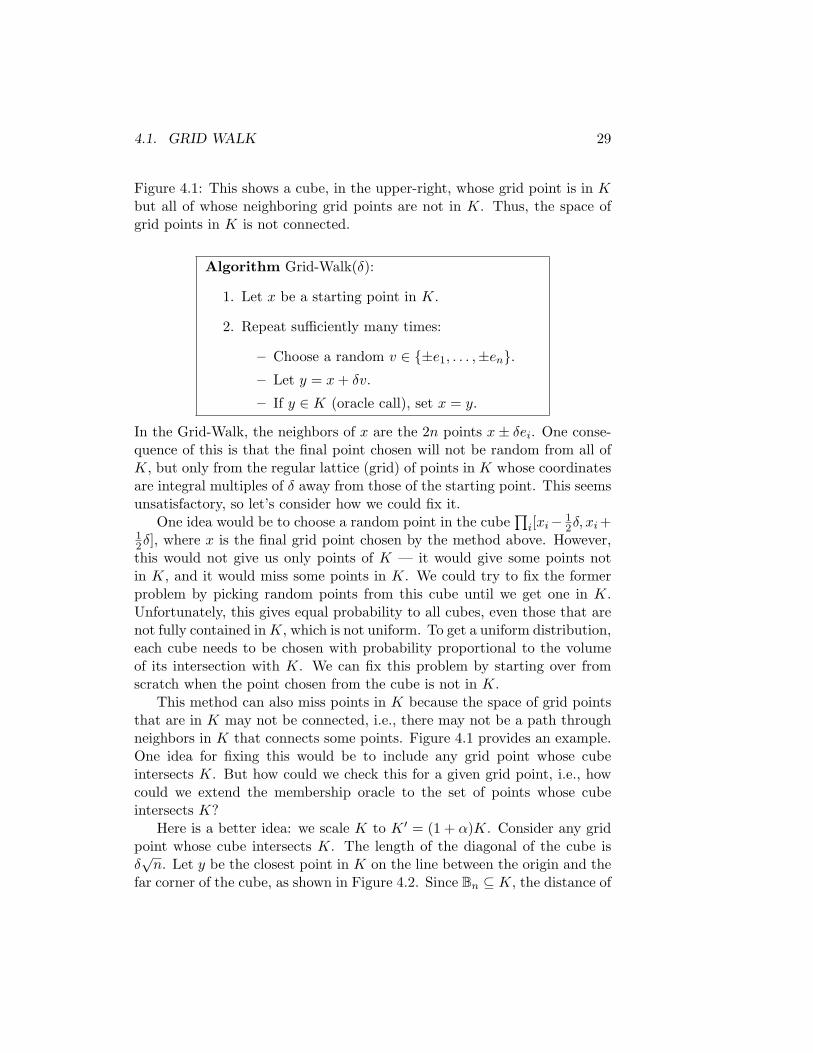
Figure 4.1: This shows a cube, in the upper-right, whose grid point is in Kbut all of whose neighboring grid points are not in K. Thus, the space ofgrid points in K is not connected.

Algorithm Grid-Walk(δ):

1. Let x be a starting point in K.

2. Repeat sufficiently many times:

– Choose a random v ∈ ±e1, . . . ,±en.– Let y = x + δv.

– If y ∈ K (oracle call), set x = y.

In the Grid-Walk, the neighbors of x are the 2n points x± δei. One conse-quence of this is that the final point chosen will not be random from all ofK, but only from the regular lattice (grid) of points in K whose coordinatesare integral multiples of δ away from those of the starting point. This seemsunsatisfactory, so let’s consider how we could fix it.

One idea would be to choose a random point in the cube∏

i[xi− 12δ, xi +

12δ], where x is the final grid point chosen by the method above. However,this would not give us only points of K — it would give some points notin K, and it would miss some points in K. We could try to fix the formerproblem by picking random points from this cube until we get one in K.Unfortunately, this gives equal probability to all cubes, even those that arenot fully contained in K, which is not uniform. To get a uniform distribution,each cube needs to be chosen with probability proportional to the volumeof its intersection with K. We can fix this problem by starting over fromscratch when the point chosen from the cube is not in K.

This method can also miss points in K because the space of grid pointsthat are in K may not be connected, i.e., there may not be a path throughneighbors in K that connects some points. Figure 4.1 provides an example.One idea for fixing this would be to include any grid point whose cubeintersects K. But how could we check this for a given grid point, i.e., howcould we extend the membership oracle to the set of points whose cubeintersects K?

Here is a better idea: we scale K to K ′ = (1 + α)K. Consider any gridpoint whose cube intersects K. The length of the diagonal of the cube isδ√

n. Let y be the closest point in K on the line between the origin and thefar corner of the cube, as shown in Figure 4.2. Since Bn ⊆ K, the distance of


Figure 4.2: This shows K, Bn inside K, and a cube that intersects K butwhose grid point is not in K. Since ‖y‖ ≥ 1 and the length L of the diagonalof the cube is δ

√n, the cube is fully contained in (1 + δ

√n)K.

y from origin is at least 1, so if we set α = δ√

n, then (1 + α)K will containall of this cube. Thus, any cube that intersects K will be fully containedin K ′. Now, consider the line between any two points x, y ∈ K. There is apath through the cubes intersecting this line that only transitions betweencubes that share a common side, i.e., whose grid points are neighbors. Everypoint on the line is in K, so every cube on the path is in K ′. This provesthat there is a path between any two grid points in K, so our state space isconnected. Another way to include all intersected cubes is to expand K toK + δ

√nBn. It is always possible to extend the membership oracle for K to

one for K + δ√

nBn.We now have a procedure that will choose a point from K uniformly

at random (provided that the final grid point is uniform — more on thisbelow). However, we may have to choose many random grid points beforethe point chosen from its cube is in K. The probability of success on eachiteration is Vol(K) divided by the volume of all the δ-cubes whose centersare in K ′. By the argument from above, every such cube is contained in(1 + α)K ′ = (1 + α)2K. So the probability of success is at least

Vol(K)Vol((1 + α)2K)

= (1 + α)−2n = (1 + δ√

n)−2n = (1 +δn√n

)−2n ≈ e−2δn√

n.

If we choose δ = 1/2n√

n (polynomial in n), then the probability of success isbounded from below by a constant, which means that the expected numberof iterations is O(1).

It remains to determine the number of steps of the random walk neededto choose a random grid point. Let C denote the set of grid points in K,and let wi be the set of points traversed by the random walk, with wi ∈ Cand w0 the starting point. Then, for any points x, y ∈ C, the probability oftransitioning from x to y, P(wi+1 = y | wi = x), is

pxy =

12n if y ∈ C ∩N (x),1− |C∩N (x)|

|N (x)| if y = x,

0 otherwise.

Notice that pxy = pyx = 1/2n if x, y ∈ C are neighbors. Now, supposethat πx were a steady state of this distribution, i.e., that the distribution

4.1. GRID WALK 31

of wi+1 is π if the distribution of wi is π. For the uniform distribution, weget πx =

∑y πypyx = πx(

∑y pyx) = πx(

∑y pxy) = πx, which shows that the

uniform distribution is a steady state. This is good, but this doesn’t provethat the random walk converges to this steady state. Perhaps there is morethan one steady state, or perhaps it doesn’t converge at all.

Suppose that we always performed a transition (i.e, pxx = 0 for allx ∈ C). Then, the transition graph would be bipartite (since the grid isbipartite), so the random walk would clearly not be able to converge tothe uniform distribution. We can see that our graph is bipartite exceptwhen we get to boundary points. So the distribution of points that could bereached by the random walk could not be uniform until we have a reasonableprobability of getting to boundary points. It turns out that this works alrightfor convex bodies. However, a more convenient approach is to modify thedistribution so that we always stay at point x with probability at least 1

2 :on every step, we first flip a coin to decide if we will try to move at all.This destroys the bipartition of the interior grid points. (In particular, thetransition matrix P becomes positive semidefinite, so all eigenvalues arenonnegative. The back-and-forth transitions of a bipartition give a negativeeigenvalue, which is then ruled out.) A random walk that stays in placewith probability 1

2 and attempt the walk with probability 12 is called lazy.

Another potential difficulty for a random walk is having a disconnectedstate space. We saw above that expanding K took care of our connectednessproblems.

Now, let’s return to the question of whether the random walk convergesto the uniform distribution. This is answered by the following classicaltheorem, whose proof uses the Perron-Frobenius theorem.

Theorem 18. If a transition matrix P is nonbipartite and irreducible, thenthe random walk tends to a unique steady state.

This does not answer the question of how fast the random walk tendsto the uniform distribution. So rather than proving this, we will prove astronger theorem that bounds the speed of convergence. For this theorem,we will need the following notation. Let Qi be the distribution of pointwi of the random walk. We define the distance between Qi and the steadystate π to be |Qi − π| = 1

2

∑x∈Ω |Qi(x)− π(x)|. The factor of 1

2 makes 1 themaximum value (this is achieved when the two distributions are disjoint).

We next define an important notion that will help bound the rate ofconvergence to the steady state.


Definition 19. For any S ⊂ Ω, let

Φ(S) =P(wi+1 ∈ S | wi ∈ S)

π(S).

Then, the conductance of Ω is

φ = minS⊂Ω

Φ(S) = minS⊂Ω, π(S)≤ 1

2

Φ(S).

Theorem 20 (Jerrum-Sinclair). Suppose we start at a discrete random walkat a point x Then,

|Qt − π| ≤ 1Q(t)

(1− φ2

2

)t

.

This theorem implies that, the “distance” to the stationary distributionfalls by a constant factor in O(1/φ2) steps. For this reason, the quantity1/φ2 is often called the mixing time. On the other hand, it is not hardto see that 1/φ is a lower bound on the number of iterations needed todecrease the distance by a constant factor since this is the expected numberof iterations required to cross the bottleneck, from S to S (consider a startingdistribution Q0 with probability 1 at w0 ∈ S).

From this theorem, we can see that the random walk will converge rapidlyto a uniform distribution when the state space has high conductance. Intu-itively, the grid points in a convex sets should have a good chance of havinghigh conductance since they avoid the bottlenecks associated with concav-ity. Before exploring this further, we will generalize Theorem 20 to arbitraryMarkov chains.

Chapter 5

Convergence of MarkovChains

A random walk is a Markov chain. We have a state space Ω and a set ofsubsets A of Ω that form a σ-algebra, i.e., A is closed under complementsand countable unions. It is an immediate consequence that A is closed undercountable intersections and that ∅,Ω ∈ A. For any u ∈ Ω and A ∈ A, wehave the one-step probability, Pu(A), which tells us the probability of beingin A after taking one step from u. Lastly, we have a starting distributionQ0 on Ω, which gives us a probability Q0(A) of starting in the set A ∈ A.

With this setup, a Markov chain is a sequence of points w0, w1, w2, . . .such that P(w0 ∈ A) = Q0(A) and

P(wi+1 ∈ A | w0 = u0, . . . , wi = ui) = P(wi+1 ∈ A | wi = ui) = Pui(A),

for any A ∈ A. A distribution Q is called stationary if, for all A ∈ A,

Q(A) =∫

u∈ΩPu(A) dQ(u).

In other words, Q is stationary if the probability of being in A is the sameafter one step. We also have a generalized version of the symmetry we sawabove in the transition probabilities (pxy = pyx). The Markov chain is calledtime-reversible if, for all A,B ∈ A,

P(wi+1 ∈ B | wi ∈ A) = P(wi+1 ∈ A | wi ∈ B).

33

34 CHAPTER 5. CONVERGENCE OF MARKOV CHAINS

5.1 Example: The ball walk

The following algorithm, called Ball-Walk, is a continuous random walk. Inthis case, the set corresponding to the neighborhood of x is Bδ(x) = x+δBn.

Algorithm Ball-Walk(δ):

1. Let x be a starting point in K.

2. Repeat sufficiently many times:

– Choose a random y ∈ Bδ(x).

– If y ∈ K, set x = y.

Here, the state space is all of the set, so Ω = K. The σ-algebra is themeasurable subsets of K, as is usual. We can define a density function forthe probability of transitioning from u ∈ K to v, provided that u 6= v:

p(u, v) =

1

Vol(δBn) if v ∈ K ∩Bδ(u),

0 otherwise.

The probability of staying at u is

Pu(u) = 1− Vol(K ∩Bδ(u))Vol(δBn)

.

Putting these together, the probability of transitioning from u to any mea-surable subset A is

Pu(A) =

Vol(A∩K∩Bδ(u))

Vol(δBn) + Pu(u) if u ∈ AVol(A∩K∩Bδ(u))

Vol(δBn) if u /∈ A.

Since the density function is symmetric, it is easy to see that the uniformdistribution is stationary. We can also verify this directly. We can computethe probability of being in A after one step by adding up the probability thatwe transition to u for each u ∈ A. Thus, after one step from the uniformdistribution dQ(u) = 1

Vol(K) du, the probability of being in A is∫u∈A Pu(u) dQ(u) +

∫u∈A

∫v∈K∩Bδ(u)\u

1Vol(δBn) dQ(v) du

=∫u∈A

(1− Vol(K∩Bδ(u))

Vol(δBn)

)dQ(u) +

∫u∈A

∫v∈K∩Bδ(u)

1Vol(δBn) dQ(v) du

=∫u∈A dQ(u) + 1

Vol(δBn)

∫u∈A

(∫v∈K∩Bδ(u) dv − Vol(K ∩Bδ(u)

)dQ(u)

=∫u∈A dQ(u)

= Q(A)

5.2. ERGODIC FLOW AND CONDUCTANCE 35

5.2 Ergodic flow and conductance

Another way to look at the one-step probability distributions is in termsof flow. For any subset A ∈ A, the ergodic flow Φ(A) is the probability oftransitioning from A to Ω \A, i.e.,

Φ(A) =∫

u∈APu(Ω \A) dQ.

Intuitively, in a stationary distribution, we should have Φ(A) = Φ(Ω \ A).In fact, this is a characterization of the stationary distribution.

Theorem 21. A distribution Q is stationary iff Φ(A) = Φ(Ω \ A) for allA ∈ A.

Proof. Consider their difference

Φ(A)− Φ(Ω \A) =∫u∈A Pu(Ω \A) dQ(u)−

∫u/∈A Pu(A) dQ(u)

=∫u∈A(1− Pu(A)) dQ(u)−

∫u/∈A Pu(A) dQ(u)

= Q(A)−∫u∈Ω Pu(A) dQ(u).

The latter quantity is the probability of staying in A after one step, soΦ(A)− Φ(Ω \A) = 0 iff Q is stationary.

Now, let’s return to the question of how quickly (and whether) this ran-dom walk converges to the stationary distribution. As before, it is convenientto make the walk lazy by giving probability 1

2 of staying in place insteadof taking a step. This means that Pu(u) ≥ 1

2 and, more generally, forany A ∈ A, Pu(A) ≥ 1

2 if u ∈ A and Pu(A) < 12 if u /∈ A. Also as before,

the notion of conductance will be useful. In this general context, we defineconductance as

φ = minA∈A, Q(A)≤ 1

2

Φ(A)Q(A)

,

where Q is the stationary distribution. This is the probability of transition-ing to Ω \A given that we are starting in A.

We use the L1 distance or total variation distance as the definition ofthe distance d(Qt, Q) between distributions:

d(Qt, Q) : |Qt −Q| = supA∈A

Qt(A)−Q(A).

We would like to know how large t must be before d(Qt, Q) ≤ 12d(Q0, Q).

This is one definition of the mixing time. It would be nice to get a bound


by showing that Qt(A) − Q(A) drops quickly for every A. This is not thecase (consider, e.g., the ball walk starting at a single point). Instead, we canlook at supQ(A)=x Qt(A)−Q(A) for each fixed x ∈ [0, 1]. A bound for everyx would imply the bound we need. To prove a bound on this by induction,we will define it in a formally weaker way. Our upper bound is

ht(x) = supg∈Fx

∫u∈Ω

g(u) (dQt(u)− dQ(u)) = supg∈Fx

∫u∈Ω

g(u) dQt(u)− x,

where Fx is the set of functions

Fx =

g : Ω → [0, 1] :∫

u∈Ωg(u) dQ(u) = x

.

It is clear that ht(x) is an upper bound on supQ(A)=x Qt(A)−Q(A) since gcould be the characteristic of A. The following lemma shows that these twoquantities are in fact equal as long as Q is atom-free, i.e., there is no x ∈ Ωsuch that Q(x) > 0.

Lemma 22. If Q is atom-free, then ht(x) = supQ(A)=x Qt(A)−Q(A).

Proof (Sketch). Consider the set of points X that maximize dQt/dQ, theirvalue density. (This part would not be possible of Q had an atom.) Putg(x) = 1 for all x ∈ X. These points give the maximum payoff per unit ofweight from g, so it is optimal to put as much weight on them as possible.Now, find the set of maximizing points in Ω \ X. Set g(x) = 1 at thesepoints. Continue until the set of points with g(x) = 1 has measure x.

In fact, this argument shows that when Q is atom-free, we can find aset A that achieves the supremum. When Q has atoms, we can includethe high value atoms and use this procedure on the non-atom subset of Ω;however, we made to include a fraction of one atom to achieve the supremum.This shows that ht(x) can be achieved by a function g that is 0− 1 valuedeverywhere except for at most one point.

Another important fact about ht is the following.

Lemma 23. The function ht is concave.

Proof. Let g1 ∈ Fx and g2 ∈ Fy. Then, we can see that αg1 + (1 − α)g2 ∈Fαx+(1−α)y, which implies that

ht(αx + (1− α)y)

≥∫

u∈Ωαg1(u) + (1− α)g2(u) dQt(u)− (αx + (1− α)y)

= α(∫

u∈Ωg1(u) dQt(u)− x) + (1− α)(

∫u∈Ω

g2(u) dQt(u)− y).


Since this holds for any such g1 and g2, it must hold if we take the sup, whichgives us ht(αx+(1−α)y) ≥ αht(x)+ (1−α)ht(y). Thus, ht is concave.

Now, we come to the main lemma relating ht to ht−1. This will allow usto put a bound on d(Qt, Q).

Lemma 24. Let Q be atom-free, and y = minx, 1− x. Then

ht(x) ≤ 12ht−1(x− 2φy) +

12ht−1(x + 2φy).

Proof. Assume that y = x, i.e., x ≤ 12 . The other part is similar. We will

construct two functions, g1 and g2, and use these to bound ht(x). Let A ∈ Abe a subset to be chosen later with Q(A) = x. Let

g1(u) =

2Pu(A)− 1 if u ∈ A,

0 if u /∈ A,and g2(u) =

1 if u ∈ A,

2Pu(A) if u /∈ A.

First, note that (12g1 + 1

2g2)(u) = Pu(A) for all u ∈ Ω, which means that

12

∫u∈Ω

g1(u) dQt−1(u) +12

∫u∈Ω

g2(u) dQt−1(u)

=∫

u∈Ω(12g1(u) +

12g2(u)) dQt−1(u)

=∫

u∈ΩPu(A) dQt−1(u)

= Qt(A)

On the other hand,

12

∫u∈Ω

g1(u) dQ(u) +12

∫u∈Ω

g2(u) dQ(u) =∫

u∈ΩPu(A) dQ(u) = Q(A)

since Q is stationary. Hence (12g1 + 1

2g2) ∈ Fx.Putting these together, wehave

12

∫u∈Ω

g1(u) (dQt−1(u)− dQ(u)) +12

∫u∈Ω

g2(u) (dQt−1(u)− dQ(u))

= Qt(A)−Q(A).


Figure 5.1: The value of ht(x) lies below the line between ht−1(x1) andht−1(x2). Since x1 ≤ x(1−2φ) ≤ x ≤ x(1+2φ) ≤ x2 and ht−1 is concave, thisimplies that ht(x) lies below the line between ht−1(x(1−2φ)) and ht−1(x(1+2φ)).

Since Q is atom-free, there is a subset A ⊆ Ω such that

ht(x) = Qt(A)−Q(A)

=12

∫u∈Ω

g1(u) (dQt−1(u)− dQ(u)) +

12

∫u∈Ω

g2(u) (dQt−1(u)− dQ(u))

≤ 12ht−1(x1) +

12ht−1(x2),

where x1 =∫u∈Ω g1(u) dQ(u) and x2 =

∫u∈Ω g2(u) dQ(u). Now, we know

that 12x1 + 1

2x2 = x. Specifically, we can see that

x1 =∫

u∈Ωg1(u) dQ(u)

= 2∫

u∈APu(A) dQ(u)−

∫u∈A

dQ(u)

= 2∫

u∈A(1− Pu(Ω \A)) dQ(u)− x

= x− 2∫

u∈APu(Ω \A) dQ(u)

= x− 2Φ(A)≤ x− 2φx

= x(1− 2φ).

This implies that x2 ≥ x(1 + 2φ). Since ht−1 is concave, the chord fromx1 to x2 on ht−1 lies below the chord from x(1 − 2φ) to x(1 + 2φ). (SeeFigure 5.1.) Therefore, ht(x) ≤ 1

2ht−1(x(1− 2φ)) + 12ht−1(x(1 + 2φ)).

Given some information about Q0, this lemma allows us to put boundson the rate of convergence to the stationary distribution.

Theorem 25. Let 0 ≤ s ≤ 1 and C0 and C1 be such that

h0(x) ≤ C0 + C1 min√

x− s,√

1− x− s.


Then

ht(x) ≤ C0 + C1 min√

x− s,√

1− x− s(

1− φ2

2

)t

.

‘

Proof. We argue by induction on t for s = 0. The inequality is true for t = 0by our hypothesis. Now, suppose that x ≤ 1

2 and the inequality holds forall values less than t. From the lemma, we know that

ht(x) ≤ 12ht−1(x(1− 2φ)) +

12ht−1(x(1 + 2φ))

≤ C0 +12C1(√

x(1− 2φ) +√

x(1 + 2φ))(1− 12φ2)t−1

= C0 +12C1

√x(√

1− 2φ +√

1 + 2φ)(1− 12φ2)t−1

≤ C0 +12C1

√x(1− 1

2φ2)t,

provided that√

1− 2φ +√

1 + 2φ ≤ 2(1 − 12φ2). The latter inequality can

be verified by squaring both sides, rearranging, and squaring again.

Corollary 26. If M = supA∈A Q0(A)/Q(A), then we have

d(Qt, Q) ≤√

M(1− 12φ2)t.

Proof. By the definition of M , we know that

h0(x) ≤ minMx, 1 − x ≤ minMx, 1.

Next, we will show that minMx, 1 ≤√

Mx. If Mx = minMx, 1, thenMx ≤ 1, which implies that Mx ≤

√Mx. If 1 = minMx, 1, then 1 ≤ Mx,

which implies that 1 ≤√

Mx ≤ Mx. So we have shown that

h0(x) ≤ minMx, 1 ≤√

Mx.

Thus, by the last theorem, we know that

d(Qt, Q) ≤ maxx

ht(x) ≤√

M(1− 12φ2)t.

Chapter 6

Sampling with the Ball Walk

A geometric random walk is said to be rapidly mixing if its conductanceis bounded from below by an inverse polynomial in the dimension. ByCorollary 26, this implies that the number of steps to halve the variationdistance to stationary is a polynomial in the dimension. The conductanceof the ball walk in a convex body K can be exponentially small. Consider,for example, starting at point x near the apex of a rotational cone in Rn.Most points in a ball of radius δ around x will lie outside the cone (if xis sufficiently close to the apex) and so the local conductance is arbitrarilysmall. So, strictly speaking, the ball walk is not rapidly mixing.

There are two ways to get around this. For the purpose of samplinguniformly from K, one can expand K a little bit by considering K ′ = K +αBn, i.e., adding a ball of radius α around every point in K. Then for α >2δ√

n, it is not hard to see that `(u) is at least 1/8 for every point u ∈ K ′.We can now consider the ball walk in K ′. This fix comes at a price. First,we need a membership oracle for K ′. This can be constructed as follows:given a point x ∈ Rn, we find a point y ∈ K such that |x− y| is minimum.This is a convex program and can be solved using the ellipsoid algorithm [?]and the membership oracle for K, Second, we need to ensure that Vol(K ′)is comparable to Vol(K). Since K contains a unit ball, K ′ ⊆ (1 + α)K andso with α < 1/n, we get that Vol(K ′) < eVol(K). Thus, we would needδ < 1/2n

√n.

Does large local conductance imply that the conductance is also large?We will prove that the answer is yes. The next lemma about one-stepdistributions of nearby points will be useful.

Lemma 27. Let u, v be such that |u− v| ≤ tδ√n

and `(u), `(v) ≥ `. Then,

||Pu − Pv||tv ≤ 1 + t− `.

41

42 CHAPTER 6. SAMPLING WITH THE BALL WALK

Roughly speaking, the lemma says that if two points with high local con-ductance are close in Euclidean distance, then their one-step distributionshave a large overlap. Its proof follows from a computation of the overlapvolume of the balls of radius δ around u and v.

We can now state and prove a bound on the conductance of the ballwalk.

Theorem 28. Let K be a convex body of diameter D so that for every pointu in K, the local conductance of the ball walk with δ steps is at least `. Then,

φ ≥ `2δ

16√

nD.

The structure of most proofs of conductance is similar and we will illus-trate it by proving this theorem.

Proof. Let K = S1 ∪ S2 be a partition into measurable sets. We will provethat ∫

S1

Px(S2) dx ≥ `2δ

16√

nDminVol(S1),Vol(S2) (6.1)

Note that since the uniform distribution is stationary,∫S1

Px(S2) dx =∫

S2

Px(S1) dx.

Consider the points that are “deep” inside these sets, i.e. unlikely tojump out of the set (see Figure 6.1):

S′1 =

x ∈ S1 : Px(S2) <`

4

and

S′2 =

x ∈ S2 : Px(S1) <`

4

.

Let S′3 be the rest i.e., S′3 = K \ S′1 \ S′2.

Figure 6.1: The conductance proof. The dark line is the boundary betweenS1 and S2.

43

Suppose Vol(S′1) < Vol(S1)/2. Then∫S1

Px(S2) dx ≥ `

4Vol(S1 \ S′1) ≥

`

8Vol(S1)

which proves (6.1).So we can assume that Vol(S′1) ≥ Vol(S1)/2 and similarly Vol(S′2) ≥

Vol(S2)/2. Now, for any u ∈ S′1 and v ∈ S′2,

||Pu − Pv||tv ≥ 1− Pu(S2)− Pv(S1) > 1− `

2.

Applying Lemma 27 with t = `/2, we get that

|u− v| ≥ `δ

2√

n.

Thus d(S1, S2) ≥ `δ/2√

n. Applying Theorem 29 to the partition S′1, S′2, S

′3,

we have

Vol(S′3) ≥ `δ√nD

minVol(S′1),Vol(S′2)

≥ `δ

2√

nDminVol(S1),Vol(S2)

We can now prove (6.1) as follows:∫S1

Px(S2) dx =12

∫S1

Px(S2) dx +12

∫S2

Px(S1) dx

≥ 12Vol(S′3)

`

4

≥ `2δ

16√

nDminVol(S1),Vol(S2).

As observed earlier, by going to K ′ = K + (1/n)Bn and using δ =1/2n

√n, we have ` ≥ 1/8. Thus, for the ball walk in K ′, φ = Ω(1/n2D)

and the mixing rate is O(n4D2).In later chapters, we will see how to improve this bound. We will also see

how to obtain a polynomial sampling algorithm, i.e., one whose dependenceon D is only logarithmic in D.

44 CHAPTER 6. SAMPLING WITH THE BALL WALK

Chapter 7

The Localization Lemma andan Isoperimetric Inequality

To formulate an isoperimetric inequality for convex bodies, we consider apartition of a convex body K into three sets S1, S2, S3 such that S1 and S2

are “far” from each other, and the inequality bounds the minimum possiblevolume of S3 relative to the volumes of S1 and S2. We will consider differentnotions of distance between subsets. Perhaps the most basic is the Euclideandistance:

d(S1, S2) = min|u− v| : u ∈ S1, v ∈ S2.

Suppose d(S1, S2) is large. Does this imply that the volume of S3 = K\(S1∪S2) is large? The classic counterexample to such a theorem is a dumbbell— two large subsets separated by very little. Of course, this is not a convexset!

The next theorem, proved in [?] (improving on a theorem in [?] by afactor of 2; see also [?]) asserts that the answer is yes.

Theorem 29. Let S1, S2, S3 be a partition into measurable sets of a convexbody K of diameter D. Then,

Vol(S3) ≥2d(S1, S2)

DminVol(S1),Vol(S2).

A limiting version of this inequality is the following: For any subset Sof a convex body of diameter D,

Voln−1(∂S ∩K) ≥ 2D

minVol(S),Vol(K \ S)

45

46CHAPTER 7. THE LOCALIZATION LEMMA AND AN ISOPERIMETRIC INEQUALITY

which says that the surface area of S inside K is large compared to thevolumes of S and K \S. This is in direct analogy with the classical isoperi-metric inequality, which says that the surface area to volume ratio of anymeasurable set is at least the ratio for a ball.

How does one prove such an inequality? In what generality does it hold?(i.e., for what measures besides the uniform measure on a convex set?) Wewill address these questions in this section.

Theorem 29 can be generalized to arbitrary logconcave measures. Itsproof is very similar to that of 29 and we will presently give an outline.

Theorem 30. Let f be a logconcave function whose support has diameterD and let πf be the induced measure. Then for any partition of Rn intomeasurable sets S1, S2, S3,

πf (S3) ≥2d(S1, S2)

Dminπf (S1), πf (S2).

In terms of diameter, this inequality is the best possible, as shown by acylinder. A more refined inequality is obtained in [?, ?] using the averagedistance of a point to the center of gravity (in place of diameter). It is pos-sible for a convex body to have much larger diameter than average distanceto its centroid (e.g., a cone). In such cases, the next theorem provides abetter bound.

Theorem 31. Let f be a logconcave density in Rn and πf be the correspond-ing measure. Let zf be the centroid of f and define M(f) = Ef (|x − zf |).Then, for any partition of Rn into measurable sets S1, S2, S3,

πf (S3) ≥ln 2

M(f)d(S1, S2)πf (S1)πf (S2).

For an isotropic density, M(f)2 ≤ Ef (|x− zf |2) = n and so M(f) ≤√

n.The diameter could be unbounded (e.g., an isotropic Gaussian).

A further refinement, based on isotropic position, has been conjecturedin [?]. Let λ be the largest eigenvalue of the inertia matrix of f , i.e.,

λ = maxv:|v|=1

∫Rn

f(x)(vT x)2 dx. (7.1)

Then the conjecture says that there is an absolute constant c such that

πf (S3) ≥c√λ

d(S1, S2)πf (S1)πf (S2).

47

7.0.1 The localization lemma

The proofs of these inequalities are based on an elegant idea: integral in-equalities in Rn can be reduced to one-dimensional inequalities! Checkingthe latter can be tedious but is relatively easy. We illustrate the main ideaby sketching the proof of Theorem 30.

For a proof of Theorem 30 by contradiction, let us assume the converseof its conclusion, i.e., for some partition S1, S2, S3 of Rn and logconcavedensity f ,∫

S3

f(x) dx < C

∫S1

f(x) dx and∫

S3

f(x) dx < C

∫S2

f(x) dx

where C = 2d(S1, S2)/D. This can be reformulated as∫Rn

g(x) dx > 0 and∫

Rn

h(x) dx > 0 (7.2)

where

g(x) =

Cf(x) if x ∈ S1,

0 if x ∈ S2,

−f(x) if x ∈ S3.

and h(x) =

0 if x ∈ S1,

Cf(x) if x ∈ S2,

−f(x) if x ∈ S3.

These inequalities are for functions in Rn. The main tool to deal with themis the localization lemma [?] (see also [?] for extensions and applications).

Lemma 32. Let g, h : Rn → R be lower semi-continuous integrable func-tions such that ∫

Rn

g(x) dx > 0 and∫

Rn

h(x) dx > 0.

Then there exist two points a, b ∈ Rn and a linear function ` : [0, 1] → R+

such that∫ 1

0`(t)n−1g((1− t)a+ tb) dt > 0 and

∫ 1

0`(t)n−1h((1− t)a+ tb) dt > 0.

The points a, b represent an interval A and one may think of l(t)n−1dAas the cross-sectional area of an infinitesimal cone with base area dA. Thelemma says that over this cone truncated at a and b, the integrals of g andh are positive. Also, without loss of generality, we can assume that a, b arein the union of the supports of g and h.


The main idea behind the lemma is the following. Let H be any halfspacesuch that ∫

Hg(x) dx =

12

∫Rn

g(x) dx.

Let us call this a bisecting halfspace. Now either∫H

h(x) dx > 0 or∫

Rn\Hh(x) dx > 0.

Thus, either H or its complementary halfspace will have positive integralsfor both g and h. Thus we have reduced the domains of the integrals fromRn to a halfspace. If we could repeat this, we might hope to reduce thedimensionality of the domain. But do there even exist bisecting halfspaces?In fact, they are aplenty: for any (n− 2)-dimensional affine subspace, thereis a bisecting halfspace with A contained in its bounding hyperplane. To seethis, let H be halfspace containing A in its boundary. Rotating H about Awe get a family of halfspaces with the same property. This family includesH ′, the complementary halfspace of H. Now the function

∫H g −

∫Rn\H g

switches sign from H to H ′. Since this is a continuous family, there mustbe a halfspace for which the function is zero, which is exactly what we want(this is sometimes called the “ham sandwich” theorem).

If we now take all (n − 2)-dimensional affine subspaces given by somexi = r1, xj = r2 where r1, r2 are rational, then the intersection of all thecorresponding bisecting halfspaces is a line (by choosing only rational valuesfor xi, we are considering a countable intersection). As long as we are leftwith a two or higher dimensional set, there is a point in its interior with atleast two coordinates that are rational, say x1 = r1 and x2 = r2. But thenthere is a bisecting halfspace H that contains the affine subspace given byx1 = r1, x2 = r2 in its boundary, and so it properly partitions the currentset. With some additional work, this leads to the existence of a concavefunction on an interval (in place of the linear function ` in the theorem)with positive integrals. Simplifying further from concave to linear takesquite a bit of work.

Going back to the proof sketch of Theorem 30, we can apply the lemmato get an interval [a, b] and a linear function ` such that∫ 1

0`(t)n−1g((1− t)a + tb) dt > 0 and

∫ 1

0`(t)n−1h((1− t)a + tb) dt > 0.

(7.3)(The functions g, h as we have defined them are not lower semi-continuous.However, this can be easily achieved by expanding S1 and S2 slightly so as to

49

make them open sets, and making the support of f an open set. Since we areproving strict inequalities, we do not lose anything by these modifications).

Let us partition [0, 1] into Z1, Z2, Z3.

Zi = t ∈ [0, 1] : (1− t)a + tb ∈ Si.

Note that for any pair of points u ∈ Z1, v ∈ Z2, |u− v| ≥ d(S1, S2)/D. Wecan rewrite (7.3) as∫

Z3

`(t)n−1f((1− t)a + tb) dt < C

∫Z1

`(t)n−1f((1− t)a + tb) dt

and ∫Z3

`(t)n−1f((1− t)a + tb) dt < C

∫Z2

`(t)n−1f((1− t)a + tb) dt.

The functions f and `(.)n−1 are both logconcave, so F (t) = `(t)n−1f((1 −t)a + tb) is also logconcave. We get,∫

Z3

F (t) dt < C min∫

Z1

F (t) dt,

∫Z2

F (t) dt

. (7.4)

Now consider what Theorem 30 asserts for the function F (t) over the interval[0, 1] and the partition Z1, Z2, Z3:∫

Z3

F (t) dt ≥ 2d(Z1, Z2) min∫

Z1

F (t) dt,

∫Z2

F (t) dt

. (7.5)

We have substituted 1 for the diameter of the interval [0, 1]. Also, d(Z1, Z2) ≥d(S1, S2)/D = C/2. Thus, Theorem 30 applied to the function F (t) contra-dicts (7.4) and to prove the theorem in general, it suffices to prove it in theone-dimensional case.

In fact, it will be enough to prove (7.5) for the case when each Zi is asingle interval. Suppose we can do this. Then, for each maximal interval(c, d) contained in Z3, the integral of F over Z3 is at least C times the smallerof the integrals to its left [0, c] and to its right [d, 1] and so one of theseintervals is “accounted” for. If all of Z1 or all of Z2 is accounted for, thenwe are done. If not, there is an unaccounted subset U that intersects bothZ1 and Z2. But then, since Z1 and Z2 are separated by at least d(S1, S2)/D,there is an interval of Z3 of length at least d(S1, S2)/D between U ∩Z1 andU ∩ Z2 which can account for more.


We are left with proving (7.5) when each Zi is an interval. Without thefactor of two, this is trivial by the logconcavity of F . To get C as claimed,one can reduce this to the case when F (t) = ect and verify it for this function[?]. The main step is to show that there is a choice of c so that when thecurrent F (t) is replaced by ect, the LHS of (7.5) does not increase and theRHS does not decrease.

algorithmic convex geometry - college of computingvempala/acg/notes.pdf · brunn-minkowski...

Documents