algorithm theoretical basis document for the osi saf 50ghz sea ice emissivity...

SAF/OSI/CDOP/DMI/SCI/MA/139 Sea ice emissivity ATBD

EUMETSAT OSI SAF 1

Ocean and Sea Ice SAF

Algorithm theoretical basis document for the OSI SAF 50GHz sea ice emissivity model

OSI-404

Version 1.1 - Oct. 2011

Rasmus T. Tonboe Harald Schyberg


EUMETSAT OSI SAF 2

Document change record:

Document Version Date Authors Description v1.0 Dec. 2010 R. Tonboe and H.

Schyberg For review

v1.1 Oct. 2011 Response to review comments


EUMETSAT OSI SAF 3

Table of contents: 1. Introduction ............................................................................................................................................ 5

1.1 Scope of this document .................................................................................................................... 6 1.2 Emissivity models ............................................................................................................................ 6

2. The semi-empirical emissivity model .................................................................................................... 8 3. Special Sensor Microwave Imager/Sounder (SSMIS) ........................................................................... 9 4. The cross track scanning microwave sounding unit (AMSU).............................................................. 10

5. The microwave emission model....................................................................................................... 11 6. Sea ice thermodynamic and mass model.......................................................................................... 12 7. The interface between the thermodynamic and the emission model................................................ 13

8. Algorithm Description: the emissivity model ...................................................................................... 14 8.1 Functionality of the model.............................................................................................................. 19

9. The effective temperature..................................................................................................................... 23 10. Processing........................................................................................................................................... 24 11. Validation plan ................................................................................................................................... 25 Acknowledgements .................................................................................................................................. 26 References ................................................................................................................................................ 27


EUMETSAT OSI SAF 4

Glossary AMSR - Advanced Microwave Scanning Radiometer AMSU - Advanced Microwave Sounding Unit

ATBD - Algorithm Theoretical Basis Document (This document)

CDOP – Continuous Development and Operations Phase

DMI – Danish Meteorological Institute

EUMETSAT - European Organisation for the Exploitation of Meteorological Satellites

FOV - Field of View HIRLAM - High Resolution Local Area Model

Metop – EUMETSAT OPerational METeorological polar orbiting satellite

NWP - Numerical Weather Prediction

OSISAF – Ocean and Sea Ice Satellite Application Facilities

SSM/I - Special Sensor Microwave/Imager

SSMIS - Special Sensor Microwave Imager/Sounder


EUMETSAT OSI SAF 5

1. Introduction The sea ice surface brightness temperature, Tb, is the product of the effective temperature, Teff, and the emissivity, e, i.e. Tb=Teff*e under the assumption of constant temperature and homogeneous conditions. Atmospheric absorption, emission and scattering are not included. The effective temperature is the integrated emitting layer thermometric temperature. This report describes an algorithm for deriving the 50GHz sea ice emissivity.

Atmospheric temperature sounding applications (such as NWP assimilation) near 50GHz over sea ice is the motivation for this study. English (1999, 2008) shows that nearly as much information about atmospheric humidity can be retrieved from e.g. sea ice covered regions as over the open ocean if the emissivity is less than 0.95, the emissivity uncertainty is less than 2 %, and the skin temperature uncertainty is less than 2 K. These accuracies have been difficult to achieve in practise over sea ice. However, test runs with the regional NWP model HIRLAM where satellite microwave radiometer data from sea ice covered regions were assimilated indicated that atmospheric temperature sounding over sea ice is in fact feasible. The test runs were using a simple sea ice surface emissivity model and it showed that the assimilation of AMSU near 50 GHz temperature sounding data improved model skill on common variables such as surface temperature, wind and air pressure (Heygster et al., 2009). The sea ice effective temperature is also important for the atmospheric sounding applications (English, 2008). The effective temperature is described in Tonboe et al. (2011) and recommendations are also given in this report.

Transmission of microwave radiation through the atmosphere in the range from 6 to 183 GHz is affected primarily by three processes: 1) oxygen absorption particularly from 50 to70 GHz and near 118 GHz, 2) water vapour absorption especially near 22 GHz and 183 GHz, and 3) scattering from water and ice particles in particular at higher frequencies and dependent on the incidence angle i.e. path length through the atmosphere. Near the 183 GHz water and the 50-70 GHz and 118 GHz oxygen absorption lines the atmosphere is virtually opaque and the satellite channels measuring at or near these frequencies are called sounding channels. However, there is a potential contribution from the surface at the lower temperature sounding frequencies between 50.3 and 54.4 GHz where microwave penetration is into the troposphere. These frequencies correspond for example to channels 3-6 on the Advanced Microwave Sounding Unit (AMSU) instrument and the channels between 50.3 and 54.4GHz on the Special Sensor Microwave Imager/ Sounder (SSMIS). The polar atmosphere is generally transparent for microwave radiation in between the sounding channels called the atmospheric windows near 18, 36, 90, and 150 GHz. For typical polar atmospheric states the down-welling emission at the surface is about 5-15 K at 18 GHz, 20-40 K at 36 GHz, 30-100 K at 89 GHz. The sea ice surface emission is typically 150-260 K for comparison. The sea ice emissivity, at a certain polarisation, frequency and angle with respect to the surface, is a function of subsurface extinction and reflections between snow layers with different permittivity. The microwave penetration depth in snow and ice is in the order of centimetres to decimetres due to significant extinction in the snow and absorption in saline ice. Physical models relate the emissivity with the snow and ice properties such as density, temperature, snow crystal and brine inclusion size to microwave attenuation, scattering and reflectivity. The brightness temperatures measured at each frequency have different spatial resolution on the Earth surface. In particular there are large differences between the 6 GHz resolution on AMSR (FOV 74 x 43 km = 3064 km2) used for ice temperature estimation and the 18 to 36 GHz (FOV 27 x 16 km = 864 km2 and 14 x 8 km = 486 km2) brightness temperatures used for deriving the emissivity.


EUMETSAT OSI SAF 6

1.1 Scope of this document This Algorithm Theoretical Basis Document describes the computational steps for a sea ice emissivity model which is implemented as part of the EUMETSAT OSISAF programme. The document introduces and justifies the scientific assumptions and choices which are made. It does not deal with all aspects of the processing. Important issues for example resolution matching, atmospheric correction of brightness temperatures, output format and quality control are not part of this document. These things are described in the reference documents: The OSI-PRD-PRO-205 in the OSI SAF Product Requirement Document referred to as [RD.1]. The validation results are presented in the validation report referred to as [RD.2]. The data are presented in the product users manual referred to as [RD.3]

General information on the EUMETSAT OSI SAF and the reference documents are available from the OSI-SAF official web site: www.osi-saf.org.

1.2 Emissivity models The sea ice surface emissivity at 50GHz is high compared to the open ocean for most ice types and penetration through the atmosphere at humidity sounding channels can be significant because the Arctic atmosphere is often very dry. Getting a good estimate of sea ice emissivity is more complicated than over the open ocean. Compared to the open ocean microwave emissivity the complications for sea ice are that there are large vertical and lateral surface heterogeneity within the foot-print including significant microwave penetration into the snow and ice and across the temperature gradient beneath the surface meaning that the surface temperature is not synonymous with the effective temperature. NWP models don't typically contain as state variables the parameters necessary to drive microwave emission models. The sea ice is dynamic: it drifts, deforms, melts or forms with significant changes from day to day which means that emissivity climatology is not as valid as it is over land without snow cover.

For smooth soil surfaces the surface reflectivity is specular, otherwise for rough surfaces the specular model can be adjusted using a single-parameter (roughness) model (Ulaby et al. 1982, p. 889) i.e.

( ) ( ) θθθ2cos',, h

sp eprpr −= (1),

where r is the reflectivity at incidence angle θ and v or h polarisation p. The subscript sp is for specular and h' is a roughness parameter.

Several models link the physical snow and ice properties with the microwave emission (e.g Tonboe et al. 2006; Weng et al. 2001). The community microwave emission model for land surfaces uses a combination of rough and specular surface scattering where the surface roughness state is derived from auxiliary parameters e.g. land use maps (Drusch et al., 2009).

Mätzler and Rosenkranz (2007) describe the bistatic scattering near Dome C in Antarctica and compare with AMSU A measurements at 31 and 50GHz. They find that the snow surface scattering is diffuse and that the Lambertian model rather than the specular model makes a good fit to measurements. This means that the angular response of the AMSU near 50GHz emissivity is small. They also find that there is a crossover between the specular and the Lambertian models near 50deg of incidence and that the Lambertian model implies that there is no polarisation difference at oblique incidence angles. However, as they mention, there is a significant polarisation difference at e.g. 19, 37 and at 89GHz and this is also


EUMETSAT OSI SAF 7

the case at 50 GHz. Mätzler (2005) simulate the emissivity of snow surfaces as a mix between Lambertian and specular scattering. However, the surface emissivity model input parameters are not prognostic variables in NWP models and they are difficult to simulate. These input parameters include, for instance, the grain size or correlation length vertical profiles within the snow-pack which are difficult to measure in the field and are a stretch target for detailed process models at present. In addition, most atmospheric models treat the surface as purely specular with the exception of that used by Guedj et al. (2010).


EUMETSAT OSI SAF 8

2. The semi-empirical emissivity model Therefore, the microwave emissivity near 50GHz is characterised here using a model where the emissivity at 50º is a function of the spectral gradient and the polarisation ratio measured at the neighbouring atmospheric window frequencies at 18 and 36 GHz. The PR and GR can be measured with SSM/I, AMSR and SSMIS sensors currently in orbit. Output from a combined 1D thermodynamic and a microwave emission model is used for generating the relationships between the emission at 50 GHz at 50º of incidence and the 18 GHz and 36 GHz simulated brightness temperatures. The approaches of both the community model (Drusch et al., 2009) and Mätzler's model (Mätzler, 2005) find solutions between two extreme cases. Similarly this model can attain solutions in between: 1) perfectly diffuse emission where there is no angular dependence and no polarisation difference similar to the model used in Heygster et al. (2009), and 2) the specular reflection with the angular dependence and the polarisation determined by the Fresnel reflection coefficients and a surface permittivity of 3.5 which is typical for sea ice. The model is expected to be valid for incidence angles between 0º and 60º and cases in between the two extremes.

Brightness temperatures are measured at window frequencies where the sensitivity to the atmosphere is minimized e.g. at 18 and 36 GHz. The spectral gradient (GR1836) is given by the following equation:

1836

18361836vv

vv

TT

TTGR

+−

= (2).

The normalisation reduces the GR sensitivity to effective temperature, and ice concentration algorithms use it to correct for first- and multiyear ice types with different volume scattering magnitudes (Comiso et al., 1997). Though the sensitivity to temperature (Teff) is reduced in GR there is still a reminiscent due to different microwave penetration at 18 and 36 GHz across the temperature gradient in snow and ice.

The polarisation ratio at 36 GHz, PR36, is given by the difference over the sum of the Tv36 and Th36 brightness temperatures at 36GHz, i.e.

3636

363636hv

hv

TT

TTPR

+−

= (3).

Also for the polarisation ratio the temperature dependence is minimized by the normalisation.


EUMETSAT OSI SAF 9

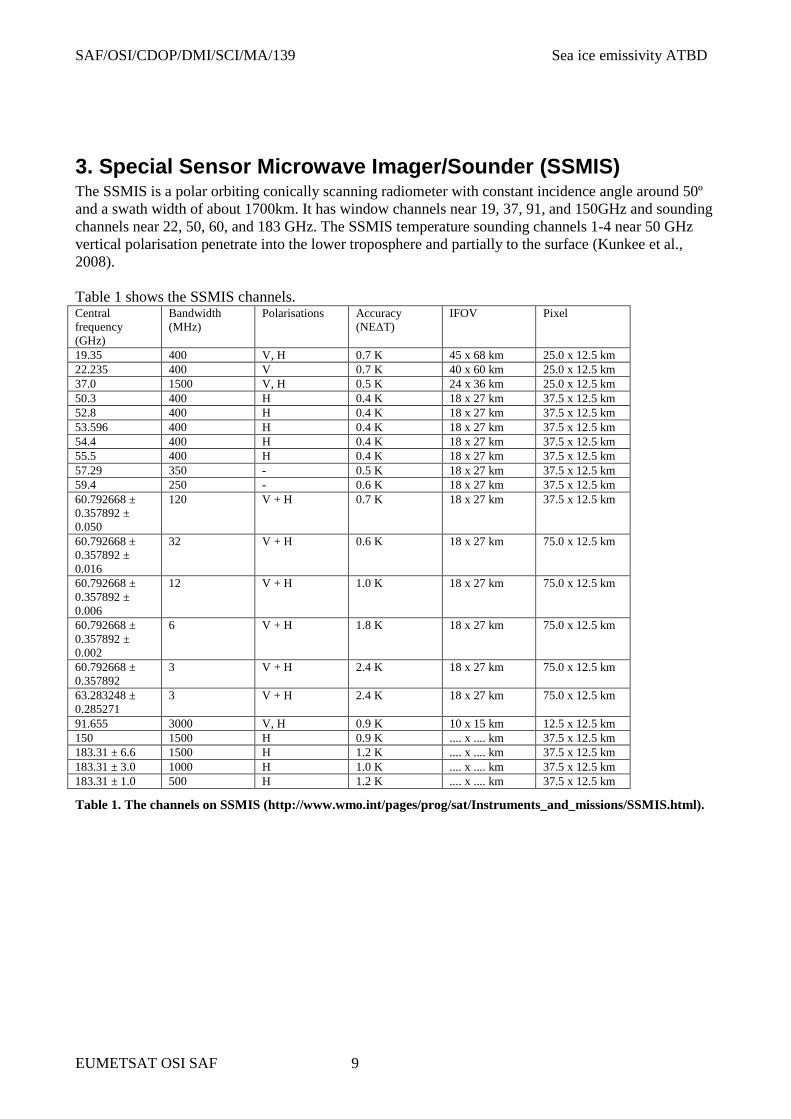
3. Special Sensor Microwave Imager/Sounder (SSMIS) The SSMIS is a polar orbiting conically scanning radiometer with constant incidence angle around 50º and a swath width of about 1700km. It has window channels near 19, 37, 91, and 150GHz and sounding channels near 22, 50, 60, and 183 GHz. The SSMIS temperature sounding channels 1-4 near 50 GHz vertical polarisation penetrate into the lower troposphere and partially to the surface (Kunkee et al., 2008). Table 1 shows the SSMIS channels. Central frequency (GHz)

Bandwidth (MHz)

Polarisations Accuracy (NE∆T)

IFOV Pixel

19.35 400 V, H 0.7 K 45 x 68 km 25.0 x 12.5 km 22.235 400 V 0.7 K 40 x 60 km 25.0 x 12.5 km 37.0 1500 V, H 0.5 K 24 x 36 km 25.0 x 12.5 km 50.3 400 H 0.4 K 18 x 27 km 37.5 x 12.5 km 52.8 400 H 0.4 K 18 x 27 km 37.5 x 12.5 km 53.596 400 H 0.4 K 18 x 27 km 37.5 x 12.5 km 54.4 400 H 0.4 K 18 x 27 km 37.5 x 12.5 km 55.5 400 H 0.4 K 18 x 27 km 37.5 x 12.5 km 57.29 350 - 0.5 K 18 x 27 km 37.5 x 12.5 km 59.4 250 - 0.6 K 18 x 27 km 37.5 x 12.5 km 60.792668 ± 0.357892 ± 0.050

120 V + H 0.7 K 18 x 27 km 37.5 x 12.5 km

60.792668 ± 0.357892 ± 0.016

32 V + H 0.6 K 18 x 27 km 75.0 x 12.5 km

60.792668 ± 0.357892 ± 0.006

12 V + H 1.0 K 18 x 27 km 75.0 x 12.5 km

60.792668 ± 0.357892 ± 0.002

6 V + H 1.8 K 18 x 27 km 75.0 x 12.5 km

60.792668 ± 0.357892

3 V + H 2.4 K 18 x 27 km 75.0 x 12.5 km

63.283248 ± 0.285271

3 V + H 2.4 K 18 x 27 km 75.0 x 12.5 km

91.655 3000 V, H 0.9 K 10 x 15 km 12.5 x 12.5 km 150 1500 H 0.9 K .... x .... km 37.5 x 12.5 km 183.31 ± 6.6 1500 H 1.2 K .... x .... km 37.5 x 12.5 km 183.31 ± 3.0 1000 H 1.0 K .... x .... km 37.5 x 12.5 km 183.31 ± 1.0 500 H 1.2 K .... x .... km 37.5 x 12.5 km

Table 1. The channels on SSMIS (http://www.wmo.int/pages/prog/sat/Instruments_and_missions/SSMIS.html).


EUMETSAT OSI SAF 10

4. The cross track scanning microwave sounding unit (AMSU) The AMSU instrument is a whisk broom polar orbiting microwave radiometer with variable incidence angle, foot-print size and the linear polarisations are mixed. Similar instruments have been in orbit since the 1970s. AMSU has scan angles between nadir and about +/-49º and a swath with of about 2000 km. Provided that the 3rd and 4th Stokes parameters are near 0 over sea ice the h and v polarisations are mixed as a function of scan angle, θ, on AMSU (Mathews et al., 2009):

( ) ( ) ( ) ( ) ( )shsv θθεθθεθε 22 sincos += (4), where

( )

+= θθ sinarcsin

HR

R

e

es (5).

Re is the Earths radius (6371km) and H is the height of the satellite above the surface (about 800km). The 3rd and 4th Stokes parameters are most often near zero during the cold season (Narvekar et al., 2011). Figure 1 shows the channels on AMSU A and the atmospheric absorption spectra.

Figure 1. The atmospheric absorption spectra and the channels on AMSU-A (figure from EUMETSAT homepage).


EUMETSAT OSI SAF 11

5. The microwave emission model Simulated data from a combined thermodynamic and emission model is used to derive the coefficients for the OSI SAF 50GHz emissivity model. The sea ice emission model relate physical snow and ice properties such as density, temperature, snow crystal and brine inclusion size from the thermodynamic model to microwave attenuation, scattering and reflectivity. The emission model used here is a sea ice version of MEMLS (Wiesmann and Mätzler, 1999) described in Mätzler et al. (2006). The theoretical improved Born approximation was used here, which validate for a wider range of frequencies and scatterer sizes than the empirical formulations (Mätzler and Wiesmann, 1999). Using the improved Born approximation the shape of the scatters is important for the scattering magnitude (Mätzler, 1998). We assume spherical scatters in snow when the correlation length pec, a measure of grain size, is less than 0.2 mm and the scatters are formed as cups when greater than 0.2 mm to resemble depth hoar crystals. The sea ice version of MEMLS includes models for the sea ice dielectric properties while using the same principles for radiative transfer as the snow model. Again the scattering within sea ice layers beneath the snow is estimated using the improved Born approximation. The scattering in first-year ice and multiyear ice is assumed from small brine pockets and air bubbles within the ice respectively. All simulations are at 50 degrees incidence angle similar to SSMIS and other conically scanning radiometers.


EUMETSAT OSI SAF 12

6. Sea ice thermodynamic and mass model In order to produce input to the emissivity model a one dimensional snow/ice thermodynamic model has been developed. Its purpose is not necessarily to reproduce a particular situation in time and space rather to provide realistic microphysical input to the emissivity model. Earlier thermodynamic models such as Maykut and Untersteiner (1971) or even simple degree day models (see e.g. Maykut, 1986) are useful for simulating ice thickness. However, for microwave emission modelling applications additional parameters such as temperature, density, snow grain size and ice salinity at very high vertical resolution are needed. Because the thermal conductivity is a function of temperature the model uses an iterative procedure between each time step of six hours. The thermodynamic model is fed with ECMWF ERA40 data input at these six hours intervals. In return the thermodynamic model produces detailed snow and ice profiles which are input to the emission model at each time step. This gives a picture of significant emission processes in sea ice even though the one dimensional thermodynamic model is not capturing the spatial variability of the sea ice cover caused for example by ice convergence resulting in deformation, ice divergence resulting in new-ice formation, and wind redistribution of the snow cover affecting snow depth, density and grain size. The thermodynamic model has the following prognostic parameters for each layer: thermometric temperature, density, thickness, snow grain size and type, ice salinity and snow liquid water content. Snow layering is very important for the microwave signatures therefore it treats snow layers related to individual snow precipitation events. For sea ice it has a growth rate dependent salinity profile. The sea ice salinity is a function of growth rate, u, and water salinity, Sw (Nakawo and Sinha, 1981), i.e.

)}102.4exp(88.012.0{12.0 4 uSS w ×−+= (6), The water salinity is 32 psu and the growth rate is in cm/day. Climatology indicates that there is snow on multiyear ice at the end of summer melt in September (Warren et al., 1999). Therefore, the multiyear ice simulations are initiated on 1 September with an isothermal 2.5 m ice floe with 5 cm old snow layer on top. The multiyear ice gradually grows at the six positions from 2.5 m to between 3.0 m and 3.4 m in spring and snow depths during winter range between 0.2 m and 0.5 m. The melt processes during the summer season are complicated and not sufficiently described by the thermodynamic model. Summer melt is therefore not included in this study. The thermodynamic model is further described in Tonboe (2005, 2010).


EUMETSAT OSI SAF 13

7. The interface between the thermodynamic and the emission model

Snow grain size affects both shortwave extinction in the thermodynamic model and microwave scattering in the emission model. The emission model is using pec as a measure of grain size and the optical grain diameter D0 forms the interface between the two models. There are no snow metamorphosis relationships in terms of pec so the conversion between terms is needed. It is assumed that grain size and pec evolve similarly during metamorphosis and our grain size growth model is not dependent on initial grain size. Therefore the conversion factor F is not critical. We use F=0.4 and the correlation length, pec, of new snow deposits is set to 0.07 mm which is typical for new snow (Wiesmann et al., 1998). Grain growth is not assigned to the top snow layer. Other microphysical parameters in the profile such as physical temperature, density, salinity are used directly in the emission model According to Marbouty’s (1980) temperature gradient metamorphism model for dry snow, used in the thermodynamic model, the mean grain size diameter (Dm) growth is a function of temperature gradient, temperature and density. Baunach et al. (2001) and Jordan et al. (1999) indicate that the growth rate is also a function of the initial grain size. However, as a first approximation Marbouty’s model gives a good fit to observations and for conversion to other structural parameters in the two models it is an advantage that growth rate is independent of initial size. For example, the shortwave extinction in the snow is a function of the snow density and the optical grain diameter (Do) (Brun et al., 1992). Since growth rate is independent of initial size Dm can be set equal to the diameter of equally sized spheres (D). D is related to Do by (Mätzler, 2002), i.e.

( )vDD o −= 1 (7), where

icesnowv ρρ /= (8). The ρsnow is the snow density and ρice is the ice density. The emission model is using the exponential correlation length (pec) a structural parameter of scatter size and distribution (Mätzler, 1998). Mätzler (2002) analyses different relationships between the snow structure, grain size and the correlation length. Do is related to pec for rounded grains, i.e.

oec FDp = (9), where F is 0.16 for snow grain sizes modelled with SNTHERM, 0.3-0.4 for Crocus grain sizes and types, and 0.16 for fine grained snow and 0.25 for medium grained snow using a one dimensional scattering model. It is further suggested to include the snow density, i.e.

)1(5.0 vDp oec −= (10).

For realistic snow densities between 150-400 kg/m3 the factor 0.5(1-v) is 0.28-0.41, i.e. the factor F in Eq. 9. These relationships are not strictly valid for new-snow and depth hoar where the grains are not rounded (Mätzler, 2002).


EUMETSAT OSI SAF 14

8. Algorithm Description: the emissivity model The sea ice emissivity at 50 GHz is related to the GR1836. Simulated data for both the vertical and horizontal polarisation at an incidence angle of 50º are shown in figure 1.

Figure 2. The simulated multi-year ice GR1836 vs. the e50v (black) and e50h (grey). The best fit line to the e50v is: e50v=3.16GR1836+0.97 and for e50h: e50h=2.48GR1836+0.90. The dashed lines show the +/-2%. The vertical grey

lines indicate the tie-points for first- (F) and multiyear (M) ice respectively.


EUMETSAT OSI SAF 15

Figure 3. The simulated multi-year ice horizontal GR1836 vs. the e50v (black) and e50h (grey). The best fit line to

the e50v is: e50v=3.21GR1836+0.95 and for e50h: e50h=2.54GR1836+0.89. The dashed lines show the +/-2%. The figure is the same as figure 1 except the gradient is at horizontal polarisation.

The model and the simulations are described in Tonboe (2010). Figure 3 is as Figure 2 except that it is showing the emissivity as a function of the gradient at horizontal polarisation. Lines have been fitted to the data clusters representing simple models for the emissivity, i.e. ( ) 97.0183616.3183650 += GRGRve (11), and ( ) 90.0183648.2183650 += GRGRhe (12). It is noted that both the emissivity and the polarisation difference are decreasing as a function of larger negative GR1836. Most of the simulated data points are within +/-2% of the fitted lines and the model - data RMS for vertical polarisation is 0.008 (for the southern hemisphere the RMS is 0.01) and the RMS is 0.019 for horizontal polarisation. The crossover of the fitted lines in Figure 2 is not physical and the v - h polarisation difference is always positive as illustrated in Figure 4. The GR1836 Arctic tie-points for first and multiyear ice are shown in Figure 2. The tie-points from Comiso et al. (1997) represent typical values for the two ice types respectively.


EUMETSAT OSI SAF 16

The GR1836 vs. the e50 polarisation difference is illustrated in Figure 4. This relationship is noisy and therefore the GR1836 cannot be used for deriving the polarisation difference.

Figure 4. The emissivity polarisation difference at 50GHz vs. the GR1836.

Instead we use the relationship between PR36 and PR50 shown in figure 5 where the polarisation ratio at 36 GHz is a proxy for the polarisation difference at 50 GHz. The model - data RMS for the 36GHZ polarisation ratio and the 50GHz polarisation ratio is 0.0014. The same processes determine the polarisation difference at 36 GHz and at 50 GHz.


EUMETSAT OSI SAF 17

Figure 5. The simulated sea ice PR18 in red, PR36 in black, and PR89 in green vs. the PR50.

There is a near 1:1 relationship between the polarisation ratio at 36 GHz and at 50 GHz. Using the linear relationships in figure 2 and 5 based on the simulated data it is now possible to estimate the 50 GHz emissivity at 50º incidence at vertical and horizontal polarisation in terms of GR1836 and PR36. The PR is decreasing from 19 GHz to 36 GHz to 50 GHz and to 89 GHz. Here we propose a simple model for extrapolating the GR1836 emissivity proxy and the PR36 polarisation proxy for SSMIS to the range of incidence angles (θ) and h and v polarisation on AMSU using the reflection coefficients for sea ice. The specular reflection coefficients for vertical, rv, and horizontal, rh, polarisation is given in terms of the sea ice permittivity ε (ε=3.5) and θ the angle of incidence, i.e.

( )2

2

2

sincos

sincos

θεθεθεθεθ

−+

−−=vr (13).

( )2

2

2

sincos

sincos

θεθθεθθ

−+

−−=hr (14).

If the sea ice absorption is considered as well i.e. the permittivity is 3.5+0.5j instead of 3.5, which is a high loss factor typical for warm and saline sea ice, then the difference in emissivity between permittivities 3.5 and 3.5+0.5j is less than 0.003 between 0 and 60 degrees. For 3.5 and 3.5+0.1j which


EUMETSAT OSI SAF 18

is realistic for cold ice it is less than 0.0002. These differences are small compared other uncertainties in particular during the cold season.

The 50 GHz emissivity is in terms of the two parameters S and R:

( ) ( ){ }θθ hh RrSe −= 150 (15), and

( ) ( ){ }θθ vv RrSe −= 150 (16). The RMS between the emissivity from the radiative transfer model (in Tonboe, 2011) and the model in eq. 15 and 16 at 50 degrees incidence angle is 0.0071 for horizontal polarisation and 0.0093 for vertical polarisation. In the Ulaby et al. (1982) model shown in eq. 1 R is a surface roughness parameter. Here because of the relationship between the PR36 and PR50 R is given as a function of PR36 shown in Figure 6. A 3rd degree polynomial is fitted to the simulated data (Tonboe, 2010) using least squares for the northern and southern hemisphere, i.e.

North ( ) 32 36286.936492.1136238.10000215.036 PRPRPRPRR +−+=

South ( ) 32 3693.53602.113622.10000471.036 PRPRPRPRR +−+= (17). and S as a function of GR1836 shown in Figure 7 using least squares: North 978.01836185.3)1836( += GRGRS South ( ) 96.0183613.31836 += GRGRS (18).

Figure 6. The R as a function of PR36. The line shows the fit to the simulated data.

For R = 0 the scattering at the surface is totally diffuse and for R = 1 the scattering is specular. R = 1 for PR36 = 0.11 at sea ice permittivity of 3.5.


EUMETSAT OSI SAF 19

Figure 7. The S as a function of GR1836. The line shows the fit to the simulated data.

The scattering of points around the line is because S is also a weak function of PR36, however this is neglected here.

8.1 Functionality of the model The emissivity as a function of incidence angle is shown for three cases: 1) the totally diffuse case where the PR36 = 0 in Figure 8, and 2) the specular case where PR36 = 0.11 at sea ice permittivity of 3.5 in Figure 9, and 3) the intermediate case where GR1836 = -0.08 and PR36 = 0.02 in Figure 10.

Figure 8. The totally diffuse case where PR36 = 0 and GR1836 = -0.03, The yellow line shows the eAMSU, ev and eh.


EUMETSAT OSI SAF 20

Figure 9 The specular case (R=1) where PR36 = 0.11 and GR1836 = -0.03. The yellow line shows the eAMSU, the

black full line the ev and the dotted line the eh.

Figure 10 The intermediate case where PR36 = 0.02 and GR1836=-0.08 (typical for multiyear ice). The yellow

line shows the eMSU, the black full line the ev and the dotted line the eh.

The e50v at 50º of incidence is shown in figure 11.


EUMETSAT OSI SAF 21

Figure 11. The 50GHz emissivity at vertical polarisation and at 50º incidence angle 1. Jan. 2003. The cyan rectangle is the area selected for data to figures 12 and 13.

The brightness temperature at 6, 18 and 36GHz vertically polarised AMSR channels is shown in Figure 12 for a small area north of Greenland shown with cyan in Figure 11 predominantly covered by multiyear ice.

Figure 12. Brightness temperatures, Tb, north of Greenland


EUMETSAT OSI SAF 22

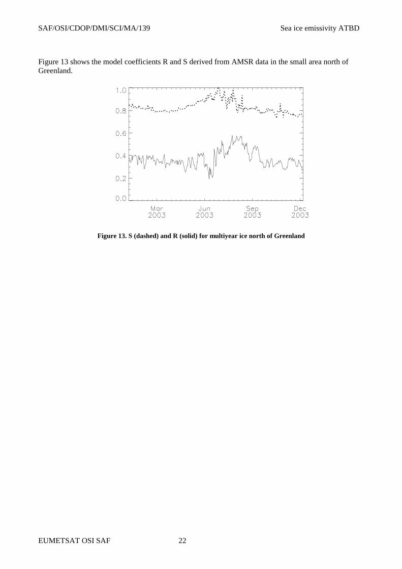
Figure 13 shows the model coefficients R and S derived from AMSR data in the small area north of Greenland.

Figure 13. S (dashed) and R (solid) for multiyear ice north of Greenland


EUMETSAT OSI SAF 23

9. The effective temperature The snow surface temperature can be measured with infrared radiometers and the effective temperature at 6 GHz can be estimated using the 6 GHz brightness temperature. Because of the large temperature gradient in the snow the snow surface temperature is relatively poorly correlated with both the snow-ice interface temperature and the effective temperatures between 6 and 89GHz. However, the effective temperatures between 6 GHz and 89 GHz are highly correlated. The 6 GHz brightness temperature can be related to the snow/ice interface temperature correcting for the temperature dependent penetration depth in saline ice. This snow-ice interface temperature estimate may be more easily used in physical modelling than the effective temperature. The 6 GHz brightness or effective temperature estimates or the snow-ice interface temperature is a closer proxy for the effective temperature near 50 GHz than the snow surface temperature (Tonboe et al. 2011). Based on the simulations in Tonboe et al. (2011) the effective temperature at 50GHz, Teff50v, is:

77.0

06.57650

−= vTvTeff (19),

where T6v is the surface brightness temperature at 6 GHz. The temperature correlation matrix is shown in Table 2 (Tonboe et al., 2011).

Table 2. The Teffv correlation matrix. The 2m air (Tair), the physical snow surface (Tsnow) and the snow-ice interface (Tice) temperatures are included.

Tair Tsnow Tice Teff6v Teff10v Teff18v Teff23v Teff36v Teff50v Teff89v Tair 1 0.97 0.78 0.75 0.76 0.77 0.78 0.80 0.84 0.91 Tsnow 0.97 1 0.81 0.78 0.79 0.80 0.81 0.84 0.88 0.95 Tice 0.78 0.81 1 0.99 0.99 0.99 0.99 0.99 0.98 0.95 Teff6v 0.75 0.78 0.99 1 0.99 0.99 0.99 0.99 0.98 0.92 Teff10v 0.76 0.79 0.99 0.9 1 0.99 0.99 0.99 0.98 0.92 Teff18v 0.77 0.80 0.99 0.99 0.99 1 0.99 0.99 0.98 0.93 Teff23v 0.78 0.81 0.99 0.99 0.99 0.99 1 0.99 0.99 0.93 Teff36v 0.80 0.84 0.99 0.99 0.99 0.99 0.99 1 0.99 0.95 Teff50v 0.84 0.88 0.98 0.98 0.98 0.98 0.99 0.99 1 0.97 Teff89v 0.91 0.95 0.95 0.92 0.92 0.93 0.93 0.95 0.97 1


EUMETSAT OSI SAF 24

10. Processing The input to the emissivity algorithm are the 18 and 36 GHz brightness temperatures from conically scanning radiometers such as SSM/I SSMIS and AMSR and the output is the R and S parameters defined in equations 12 and 13 respectively. These parameters together with a given incidence angle and polarisation can be used in equations 10 and 11 to compute the sea ice surface emissivity for atmospheric sounders such as SSMIS and AMSU-A. Input: Tb18v, Tb36v, Tb36h Summary of the 10 processing steps:

1. The NetCDF format swath data are read. 2. The 37 GHz channels are re-sampled to 19 GHz resolution using a Gaussian weighting

function and a circular 'field of view' of 56.5 km. 3. Realistic brightness temperatures for sea ice are selected for further processing:

160.0 K < Tb19v < 273.15 K 130.0 K < Tb37v < 273.15 K 100.0 K < Tb37h < 273.15 K (Tb37v - Tb19v) / (Tb37v + Tb19v) < 0.05 (Tb37v - Tb37h) / (Tb37v + Tb37h) < 0.15

4. Each of the two hemispheres is selected using each of the data point latitudes. 5. The R, S, ev and nadir e are estimated using the model. 6. Data-points where the model yields false emissivities at any angle exceeding 1 or below 0 are

excluded and flagged. 7. Each of the new data fields (R, S, ev, nadir e and flags) are appended to the swath file as

super-files and written in NetCDF format. 8. The parameters in the swath file are gridded using a nearest neighbour re-sampler. 9. The data are plotted as png-quick looks. 10. The gridded data are written as NetCDF format files.


EUMETSAT OSI SAF 25

11. Validation plan Direct in-situ measurements of surface microwave emissivity is practically expensive and difficult, and if it was done at a given point, it would have representativeness issues due to horizontal variability of the ice properties, since the emissivity product proposed in Section 4 is an average over a grid square meant to be used for comparison with large satellite footprints. We therefore propose an approach for validation where application of the product in simulation of satellite radiances is compared to real observed satellite radiances. This also fits well with the intended application of the product in sounding channel assimilation for NWP. The emissivity algorithm outlined in Section 5 will be validated by applying the emissivity product to simulation of AMSU-A lower troposphere sounding and surface microwave channel brightness temperatures. As a best guess for the state of the atmosphere, short-range forecasts of the operational short-range HIRLAM operational weather prediction model at the Norwegian Meteorological Institute will be used. The model data will be collocated with the satellite footprints and times of the real AMSU-A satellite observations. We will apply the emissivity estimate (along with an emitting temperature estimate) in the RTTOV fast radiative transfer model, given the atmospheric profile estimates at satellite observation footprints. RTTOV is a widely used radiative transfer model, particularly within the NWP community, available through EUMETSAT’s NWP SAF. We will then produce two datasets, one dataset of simulated AMSU-A satellite observations using the emissivity model, and the set of real observations for comparison. The following tasks will be undertaken:

(1) The algorithm in Section 5 will be implemented and interfaced to RTTOV calculations using the Met.no operational HIRLAM model on a regional domain containing large areas of Arctic sea ice

(2) Over areas known to be closed sea ice: (a) Determine the average sensitivity of the simulated brightness temperature to the surface

emissivity (b) Determine the average sensitivity of the simulated brightness temperatures to the efficient

surface temperature

(3) Evaluate the method by comparison of simulated brightness temperatures to real observed brightness temperatures for one or more time periods. The evaluation will be split up into regions and for instance areas of multi-year and first-year sea ice.

(4) Application of the proposed emissivity estimate will be compared to other approaches for

estimating the sounding channel ice surface emissivity: (a) Application of multi-year sea ice as predictor for emissivity, as described in Heygster el al,

2009. (b) The method applied by Mathew et al (2008) over sea ice and also devised by Karbou et al

(2006) over land, deriving emissivity directly using data from a simultaneous AMSU-A window channel measurement

This approach will ensure validation through extended time periods as well as over a widespread domain. Assessment of the sensitivity of the data to surface emissivity will provide information on how much of the scatter in the observed versus simulated data comparison can be attributed to the surface


EUMETSAT OSI SAF 26

emissivity. Comparison with alternative approaches to emissivity estimation from the same dataset will ensure that the relative merits of the different approaches are documented and that the proposed method provides an improvement on alternative approaches. A comparison of such alternative approaches was also demonstrated in Schyberg and Tveter (2009, 2010). The validation and an assessment of the accuracy of the method will be documented in a validation report.

Acknowledgements We would like to thank the two EUMETSAT reviewers Dominique Faucher and Anne O'Caroll and the two external reviewers Fatima Karbou from Meteo France and Chawn Harlow from the UK Met. Office for their constructive comments to this report. ECMWF ERA-40 data used in this study have been obtained from the ECMWF data server.The model was developed within the EU FP 7 Damocles project and its implementation, testing and validation was done within the EUMETSAT CDOP-1 OSISAF project.


EUMETSAT OSI SAF 27

References Aires, F., C. Prigent, F. Bernardo, C. Jimenez, R. Saunders, P. Brunel. 2010. A tool to estimate land

surface emissivities at microwaves frequencies (TELSEM) for use in numerical weather prediction. Q. J. R. Meteorol. Soc.

Baunach, T., C. Fierz, P. K. Satyawali, and M. Schneebeli, 2001. A model for kinetic grain growth, Annals of Glaciology 32, 1-6.

Brun, E., E. Martin, V. Simon, C. Gendre, and C. Coleou, 1989. An energy and mass model of snow cover suitable for operational avalanche forecasting. Journal of Glaciology 35(121), 333-342.

Comiso, J. C, D. J. Cavalieri, C. L. Parkinson, and P. Gloersen. 1997. Passive microwave algorithms for sea ice concentration: a comparison of two techniques. Remote Sensing of Environment 60, 357-384.

Drusch, M., T. Holmes, P. de Rosnay, G. Balsamo. 2009. Comparing ERA-40 based L-band brightness temperatures with skylab observations: a calibration/validation study using the community microwave emission model. Journal of hydrometeorology 10, DOI: 10.1175/2008JHM964.1, 213-226.

English, S. J. 1999. Estimation of temperature and humidity profile information from microwave radiances over different surface types. Journal of Applied Meteorology 38, 1526-1527.

English, S. J., The Importance of Accurate Skin Temperature in Assimilating Radiances From Satellite Sounding Instruments, IEEE Trans. Geosci. Remote Sens., vol. 46, no. 2, pp. 403 – 408, Feb. 2008.

Guedj, S., F. Karbou, F. Rabier, A. Bouchard, 2010, Microwave land emissivity over Antarctica : Impact of the surface approximation, IEEE Trans. on Geoscience and Remote sensing, Vol. 48, Issue 4, 1976-1985, 10.1109/TGRS.2009.2036254

Heygster, G., C. Melsheimer, N. Mathew, L. Toudal, R. Saldo, S. Andersen, R. Tonboe, H. Schyberg, F. Thomas Tveter, V. Thyness, N. Gustafsson, T. Landelius, and P. Dahlgren. 2009. POLAR PROGRAM: Integrated Observation and Modeling of the arctic Sea Ice and Atmosphere. Bulletin of the American Meteorological Society 90, 293 – 297.

Jordan, R., 1991. A one-dimensional temperature model for a snow cover. CRREL SP 91-16. Karbou, F., E. Gérard, and F. Rabier, 2006, Microwave Land Emissivity and Skin Temperature for

AMSU-A & -B Assimilation Over Land, Q. J. R. Meteorol. Soc., vol. 132, No. 620, Part A, pp. 2333-2355(23).

Kunkee, D. B., G. A. Poe, D. J. Boucher, S. D. Swadley, Y. Hong, J. E. Wessel, and E. A. Uliana, 2008. Design and evaluation of the first special sensor microwave imager/sounder, IEEE Transactions on Geoscience and Remote Sensing 46(4), 863-883.

Marbouty, D., 1980. An experimental study of temperature gradient metamorphosism. Journal of Glaciology 26(94), 303-312.

Mathew, N.; Heygster, G.; Melsheimer, C.; Kaleschke, L., 2008: Surface Emissivity of Arctic Sea Ice at AMSU Window Frequencies. IEEE Transactions on Geoscience and Remote Sensing, Volume 46, Issue 8 (Aug. 2008) pp 2298 – 2306.

Mätzler, C. 2005. On the determination of surface emissivity from satellite observations. IEEE Geoscience and Remote Sensing Letters 2(2), 160-163.

Mätzler, C., 1998. Improved Born approximation for scattering of radiation in a granular medium. Journal of Applied Physics 83(11), 6111-6117.

Mätzler, C., 2002. Relation between grain-size and correlation length of snow. Journal of Glaciology 48(162), 461-466.

Mätzler, C., and A. Wiesmann, 1999. Extension of the Microwave Emission Model of Layered Snowpacks to coarse-grained snow, Remote Sensing of Environment 70, 317-325.


EUMETSAT OSI SAF 28

Mätzler, C., P. W. Rosenkrantz. 2007. Dependence of Microwave brightness temperature on bistatic surface scattering: model functions and applications to AMSU-A. IEEE Transactions on Geoscience and Remote Sensing 45(7), 2130-2138.

Mätzler, C., P.W. Rosenkranz, A. Battaglia, and J.P. Wigneron, Eds., 2006. Thermal Microwave Radiation - Applications for Remote Sensing, IEE Electromagnetic Waves Series, London, UK.

Maykut, G. A., 1986. The surface heat and mass balance. In: N. Untersteiner (Ed.): The geophysics of sea ice. (pp. 395-464). NATO ASI Series, plenum Press, New York and London.

Maykut, G. A., and Untersteiner, N, 1971., Some results from a time-dependent thermodynamic model of sea ice. J. Geophys. Res., 76, 1550-1575.

Nakawo, M., and N. K. Sinha, 1981. Growth rate and salinity profile of first-year sea ice in the high Arctic. Journal of Glaciology 27(96), 315-330.

Narvekar, P. S., G. Heygster, R. Tonboe, T. J. Jackson. 2011. Analysis of WindSat third and fourth Stokes components over Arctic sea ice. IEEE Transactions on Geoscience and Remote Sensing 49(5), 1627-1636.

Schyberg, H and Tveter, F.T., 2009: Report on microwave ice surface emission modelling using NWP model data. DAMOCLES deliverable report D1.2-02.f, April, 2009. Available from the authors at Norwegian Meteorological Institute, P.O. Box 43-Blindern, NO-0313 Oslo, Norway.

Schyberg, H and Tveter, F.T., 2010: Improved assimilation method in NWP and impact on forecast quality in the Arctic. DAMOCLES deliverable report D4.3-09, June, 2010. Available from the authors at Norwegian Meteorological Institute, P.O. Box 43-Blindern, NO-0313 Oslo, Norway.

Tonboe, R. T. 2010. The simulated sea ice thermal microwave emission at window and sounding frequencies. Tellus 62A, 333-344.

Tonboe, R. T. G. Dybkjær, J. L. Høyer. 2011. Simulations of the snow covered sea ice surface and microwave effective temperature. Tellus 63A, 1028-1037.

Tonboe, R. T., 2005. A mass and thermodynamic model for sea ice. Danish Meteorological Institute Scientific Report 05-10.

Ulaby, F. T., R. K. Moore, A. K. Fung. 1982. Microwave remote sensing, active and passive, vol. II, Artech House, Norwood MA.

Warren, S. G., I. G. Rigor, N. Untersteiner, V. F. Radionov, N. N. Bryazgin, Y. I. Aleksandrov, and R. Colony, 1999. Snow depth on Arctic sea ice. Journal of Climate 12, 1814-1829.

Weng, F., B. Yan, N. C. Grody. 2001. A microwave land emissivity model. Journal of Geophysical Research 106(D17), 20115-20123.

Wiesmann, A., and C. Mätzler, 1999. Microwave emission model of layered snowpacks, Remote Sensing of Environment 70, 307-316.

Wiesmann, A., C. Fierz, and C. Mätzler, 2000. Simulation of microwave emission from physically modelled snowpacks. Annals of Glaciology 31, 397-404.

Wiesmann, A., C. Mätzler, and T. Weise, 1998. Radiometric and structural measurements of snow samples. Radio Science 33(2), 273-289.

algorithm theoretical basis document for the osi saf 50ghz sea ice emissivity...

Documents