algorithm implementation in fpgas demonstrated a thesis

Algorithm Implementation in FPGAs Demonstrated

Through Neural Network Inversion on the SRC-6e

A Thesis Submitted to the Graduate Faculty of

Baylor University

in Partial Fulfillment of the

Requirements for the Degree

of

Masters of Science

By

Paul D. Reynolds

Waco, Texas

May 2005

iii

TABLE OF CONTENTS

List of Figures ............................................................................................................... v List of Tables ................................................................................................................ vi Acknowledgments......................................................................................................... vii Dedication..................................................................................................................... viii Chapter One .................................................................................................................. 1

Introduction............................................................................................................... 1 Chapter Two.................................................................................................................. 2

The SRC-6e Reconfigurable Computer .................................................................... 2 Hardware Architecture.......................................................................................... 2 SRC-6e Development Environment ..................................................................... 4 Hardware Description Language Implementation ................................................ 5

Chapter Three................................................................................................................ 7 The Acoustic Algorithm ........................................................................................... 7

The Neural Network ............................................................................................. 7 Particle Swarm Optimitzation............................................................................... 8

Chapter Four ................................................................................................................. 10 Neural Network Accuracy and Sigmoid ................................................................... 10

From Floating to Fixed Point................................................................................ 11 The Sigmoid Approximation ................................................................................ 14

Look Up Table Implementation........................................................................ 14 Shift-add Implementation ................................................................................. 15 The Neural Network ......................................................................................... 18 Taylor Segments Approximation...................................................................... 22

Comparison Summary .......................................................................................... 24 Chapter Five.................................................................................................................. 27

Neural Network Implementations............................................................................. 27 Serial Implementation........................................................................................... 27 Parallel Node Implementation .............................................................................. 28 Parallel Input Implementation .............................................................................. 32 Conclusions on Neural Network Implementations ............................................... 33

Chapter Six.................................................................................................................... 35 Particle Swarm Implementation................................................................................ 35

Deterministic Particle Swarm ............................................................................... 35 Randomization ...................................................................................................... 37

Linear Feedback Shift Register......................................................................... 37 Squared Decimal Implementation..................................................................... 40 Particle Swarm Randomness Results................................................................ 42

Conclusions on Particle Swarm Implementation.................................................. 42 Chapter Seven ............................................................................................................... 45

Algorithm Speedup through FPGA Implementations .............................................. 45 Parallel-able .......................................................................................................... 45

iv

Pipeline-able ......................................................................................................... 47 Memory Transfer .................................................................................................. 49 Speed Ratio ........................................................................................................... 50

Appendices.................................................................................................................... 52 Appendix A................................................................................................................... 53

Parallel Input Network and Swarm Code ................................................................. 53 Main.c ................................................................................................................... 53

Appendix B ................................................................................................................... 60 Parallel Input Network and Swarm Code ................................................................. 60

Makefile ................................................................................................................ 60 Apeendix C ................................................................................................................... 62

Parallel Input Network and Swarm Code ................................................................. 62 Swarm.mc ..................................................................................................................... 62 Appendix D................................................................................................................... 69

Parallel Input Network and Swarm Code ................................................................. 69 Fitness.mc ..................................................................................................................... 69 Appendix E ................................................................................................................... 74

Parallel Input Network and Swarm Code ................................................................. 74 Blkbox.v................................................................................................................ 74

Appendix F.................................................................................................................... 78 Parallel Input Network and Swarm Code ................................................................. 78

Macros.inf ............................................................................................................. 78 Appendix G................................................................................................................... 82

Parallel Input Network and Swarm Code ................................................................. 82 Moveit.vhd............................................................................................................ 82

Appendix H................................................................................................................... 85 Parallel Input Network and Swarm Code ................................................................. 85

Squash.vhd ............................................................................................................ 85 Bibliography ................................................................................................................. 123

v

LIST OF FIGURES

Figure 1: The SRC-6e Block Diagram....................................................................... 3 Figure 2: Accuracy Sweep of Squashing Function.................................................... 12 Figure 3: Accuracy Sweep of Weights ...................................................................... 13 Figure 4: Accuracy Sweep of all Fractional Bits ....................................................... 13 Figure 5: The Block Diagram for a Lookup Table Implementation of the Sigmoid . 15 Figure 6: The Block Diagram for a Shift-Add Implementation of the Sigmoid........ 16 Figure 7: VHDL Approximation of Shift and Add Squashing Function................... 17 Figure 8: Comparison of Shift-Add FPGA Output with Real Output ....................... 17 Figure 9: A Piecewise Linear Approximation of the Sigmoid .................................. 18 Figure 10: VHDL Approximation of CORDIC Squashing Function .......................... 20 Figure 11: The Block Diagram for a CORDIC Implementation of the Sigmoid......... 21 Figure 12: Comparison of CORDIC FPGA Output and Real Output ......................... 22 Figure 13: The Block Diagram for a Taylor Series Implementation of the Sigmoid .. 23 Figure 14: VHDL Approximation ............................................................................... 24 Figure 15: Comparison of FPGA Output with Real Output ........................................ 24 Figure 16: The Block Diagram for the Serial Implementation of a Neural Network .. 28 Figure 17: The Parallel Node Implementation with Four Parallel Nodes. .................. 30 Figure 18: Parallel Node Implementation with Sixteen Multiplies ............................. 31 Figure 19: A Simplified Block Diagram of a Node Parallel Implementation. ............ 33 Figure 20: Particle Swarm with and without Randomness.......................................... 36 Figure 21: Deterministic Particle Swarm Block Diagram. .......................................... 37 Figure 22: Histograms for a LFSR Implementation and a Uniform Random Variable 39 Figure 23: Output Streams and Frequency Spectra f or a LFSR Implementation and a

Uniform Random Variable. ........................................................................ 39 Figure 24: Histograms for a Squared Decimal Implementation and a Uniform Random

Variable....................................................................................................... 41 Figure 25: Output Streams and Frequency Spectra f or a Squared Decimal

Implementation and a Uniform Random Variable...................................... 41 Figure 26: Particle Swarm Results Maximizing a Specified Area .............................. 43 Figure 27: Particle Swarm Results Maximizing a Specified Area .............................. 44

vi

LIST OF TABLES

Table 1: Segments Used for the Shift-Add Approximation......................................... 16 Table 2: CORDIC Initializing Segments ..................................................................... 21 Table 3: Taylor Series Segments and Coefficients ...................................................... 23 Table 4: A Comparison of Approximations................................................................. 25

vii

ACKNOWLEDGMENTS

I would like to thank Dr. Russell Duren and Dr. Robert Marks for providing me

with this topic to work on as well as for helping me think of ideas for some portions of

the problem. I’d also like to thank Dan Zulaica and David Caliga for helping me to

figure out some errors in my programming and giving me hints on how to use the

computer. I would also like to thank Burton Ottewell for doing some initial work on the

SRC-6e from which I could learn.

viii

DEDICATION

To my parents, who let me graduate free of debt

1

CHAPTER ONE

Introduction

The hardware implementation of algorithms can be a difficult process. An

algorithm takes a given input and produces an output based on several calculations.

Unlike state machines, an input can only produce one output, and a design could be

implemented as purely combinational logic. This, however, would be very complex and

likely have several timing issues. It is much more effective and organized to divide an

algorithm into several clocked segments. This way, the correct data will arrive at

components at the proper time and the arrival of a valid output is highly predictable.

Algorithms also tend to be too large for every calculation to be performed by

different hardware components. Implementation of large algorithms requires that many

components be reused during computation and therefore some method of control. State

machines are not required; usually a simple series of counters is sufficient.

The example presented is of neural network inversion. This thesis begins with a

brief introduction to the hardware and programming environment. Chapter three

introduces the algorithm being implemented as well as the problem background.

Chapters four, five and six describe implementations of the three inversion sub-

algorithms as well as the adaptations required for hardware. The final chapter explains

how hardware implementations are in effective decreasing algorithm computation time.

The appendices present the code for the final implementation of hardware neural network

inversion.

2

CHAPTER TWO

The SRC-6e Reconfigurable Computer

The SRC-6e Reconfigurable Computer, from here on referred to as the SRC-6e, is

a specialized system designed for the implementation of code in reconfigurable hardware.

The system contains two reconfigurable chips accessible by core processors. The chips

are programmed using languages tailored specifically for the system.

The SRC-6e has previously been used for applications by the Naval Postgraduate

School in implementing CORDIC functions [1, 2], certain RADAR applications [3], as

well as with Triple DES [4]. A group in Washington, D.C. used the SRC-6e for work

with cryptosystems [5].

Hardware Architecture

The SRC-6e contains two Pentium 3 microprocessors running at one gigahertz

and two Xilinx XC2V6000 field programmable gate arrays(FPGA) running at one

hundred megahertz. The XC2V6000 contains pre-configured logic blocks in order to

simplify the implementation of some designs. Each XC2V6000 contains 144 eighteen-bit

multiplier blocks and 144 eighteen-kilobit random memory access blocks. In addition to

pre-defined logic, each chip has approximately six million user-definable logic gates [6].

In order for the hardware to be useful, it must be able to read and write to memory

used by the main processors. For this purpose, there are six on-board memory blocks.

Each block contains four megabytes of memory, accessible by either FPGA. The

processors can access this memory through an on-board controller. The controller can

3

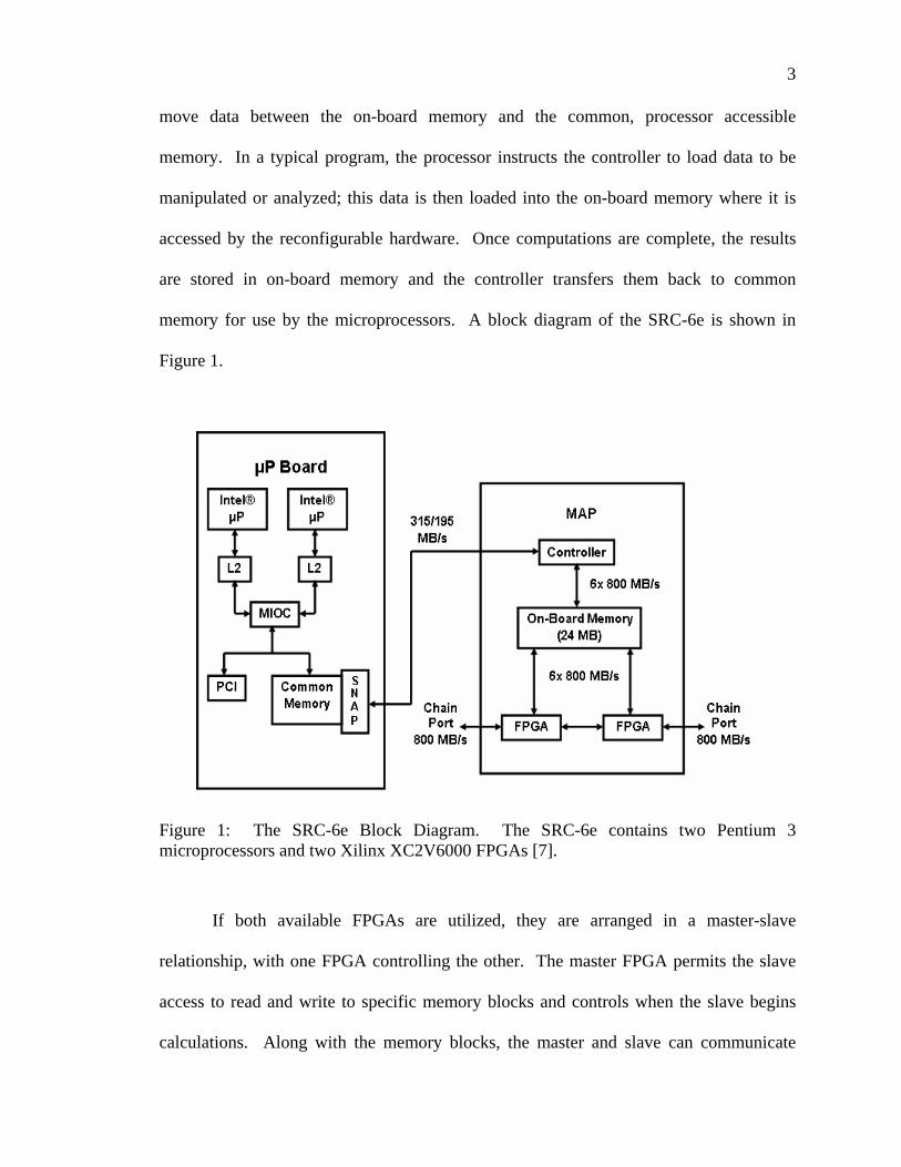
move data between the on-board memory and the common, processor accessible

memory. In a typical program, the processor instructs the controller to load data to be

manipulated or analyzed; this data is then loaded into the on-board memory where it is

accessed by the reconfigurable hardware. Once computations are complete, the results

are stored in on-board memory and the controller transfers them back to common

memory for use by the microprocessors. A block diagram of the SRC-6e is shown in

Figure 1.

Figure 1: The SRC-6e Block Diagram. The SRC-6e contains two Pentium 3 microprocessors and two Xilinx XC2V6000 FPGAs [7].

If both available FPGAs are utilized, they are arranged in a master-slave

relationship, with one FPGA controlling the other. The master FPGA permits the slave

access to read and write to specific memory blocks and controls when the slave begins

calculations. Along with the memory blocks, the master and slave can communicate

4

directly through three sixty-four bit ports. Once both FPGAs have completed

calculations, the master regains control of all six memory blocks and the controller copies

the results to common memory [7].

SRC-6e Development Environment

The SRC-6e has its own development environment and uses several programming

languages for design implementation. The SRC-6e runs a Linux operating system and is

controlled remotely via x-windows or a command line interface. At the highest level of

an implementation, the main program is written in the standard C language and executes

on the Intel processors. The main program executes as with any other platform, and the

command line and console can be used for user input or data display. From the main

program, the reconfigurable hardware is accessed in the same manner as a function. The

hardware function handles the necessary data transfers and execution on the hardware.

The hardware functionality is programmed in a modified C or FORTRAN, which

is translated by the SRC-6e compiler into Verilog code, which is then synthesized and

encoded into FPGA bit streams using standard FPGA design tools. The hardware

generation process is hidden from the programmer who simply issues a make command

to generate the compiled and synthesized program.

The high level languages can be used exclusively by themselves or along with

functions written in one of two standard hardware description languages, VHDL or

Verilog. Hardware description languages are used when more control is desired over the

FPGA circuitry. The design for the example used in this thesis was coded using a

combination of C and VHDL. It is also possible to use intellectual property cores in a

design. The core can be called from the VHDL or Verilog code and the precompiled core

5

file uploaded to the SRC-6e. The compiler will properly connect the design. This

method is used for the division operation shown in the CORDIC portion of the example.

Hardware Description Language Implementation

Hardware description languages are especially useful to gain more control of

parallel processes as well as to circumvent some of the idiosyncrasies of the higher level

programming languages. For example, the compiler will often add latency to loops

during compilation for implementation. This can be difficult to fix in the higher level

languages, though the solution may be quite obvious at the hardware description level.

One particularly frustrating peculiarity is the implementation of multipliers. For all

multiply commands, the complier requires three multipliers to be used, though typically

one is sufficient. The compiler’s multipliers also are intended for integers. For a fixed

point design, the decimal point must be moved after every multiply. This is much easier

to implement at the hardware description level.

To use hardware description languages, a module is written in either VHDL or

Verilog and then is called as a function from the C or FORTRAN hardware code. In

order for the complier to know how the higher level programming languages will

communicate with the function, two additional files must be created. In the files, the

function inputs and outputs are listed along with their order and sizes as well as the nature

of the function. The compiler needs to know when it is able to send inputs and when to

retrieve outputs. The programmer must define whether the function is stateful, external,

pipelined, or periodic as well as its latency as described in the SRC C reference guide.

In some instances, such as the following problem presented, some of the high-

level language idiosyncrasies force much of the logic to be performed in the hardware

6

description languages. However, the resulting function will not fit into any of the

predefined function characteristics. In order to circumvent this problem, the function can

be defined as functional with a pipelined structure and placed in a loop. In order for the

technique to work, the loop must be programmed so that the compiler will not add

latency. The latency is assigned as the time from when the last input enters to the time

the last output calculation is finished. Then, from the high level language side, if the

number of inputs differs from the number of outputs, pseudo-inputs can be used to fill the

extra clocks if there are more outputs than inputs or additional outputs can be ignored if

the reverse is true.

7

CHAPTER THREE

The Acoustic Algorithm

Given a set of sonar system parameters and environmental parameters, the

acoustical state of an underwater environment can be predicted by computationally

intensive computer models. It is desirable to be able to perform an inversion on the

system: given the state of the underwater environment and some fixed parameters,

determine the other input parameters to achieve optimal sonar performance. Inversion is

performed by testing many different sets of the variable input parameters and choosing

the set that mostly closely matches the desired acoustical state. In order to perform the

inversion in real time, the computation time of the model must be small and the number

of sets of unknown parameters tested kept at a minimum.

Previous work with the acoustic model has been performed by the University of

Washington and the Jet Propulsions Laboratory. Some of their work can be found in [8],

[9], and [10].

The Neural Network

In order to decrease the calculation time of the forward computation, an artificial

neural network was trained using data from the acoustic model. The network has a 27-

40-50-70-1200 architecture, with the 27 inputs corresponding to the sonar system and

environmental parameters and the 1200 outputs corresponding to the acoustic state of

water at points on an 80 by 15 grid [11].

8

The three hidden layer network greatly decreases forward computation time, from

a few minutes using the acoustic model, to few milliseconds. Though this speed is

acceptable for real-time forward calculations, it is too slow to produce a real-time

inversion. By using a parallel FPGA implementation, computation time can be decreased

enough to make real-time inversion possible.

Particle Swarm Optimization

In order to minimize the number of sets of unknown parameters tested, a particle

swarm optimization is used. Particle swarm optimization employs several agents

exploring a multi-dimensional search space to maximize a given fitness function. As the

agents traverse the space, they have tendencies to return to their own previous best

locations as well as to the best location of the group. The tendency is based on the

distance from the best locations and some uniform randomness. The update equations

are:

])[(])[(][]1[][][]1[

2211

0

kXGRCkXPRCkVkVkVAkXkX

−+−+=++=+

The next location, X[k+1], and next velocity, V[k+1] of each agent are

determined using the following: X[k], the current location; V[k], the current velocity; A0,

an update constant controlling the resolution of movement; C1 and C2, bias coefficients;

R1 and R2, uniform random variables between 0 and 1; P, the personal best fitness

location and G, the group best fitness location.

For the above neural network inversion, the fitness function is defined as the sum

of the differences in pixels in the calculated acoustical state and the desired state. A

smaller sum is considered to have a higher fitness. To prove that the inversion method is

9

viable, a known achievable set of outputs is used as the desired state. If the inputs found

by the inversion produce approximately the same set of outputs, then the method can be

used to invert a set of desired outputs that lie outside the achievable set with confidence

that nearly the closest attainable set is found.

Certain frequently used limits are also applied to the particle swarm. Velocity is

limited to help keep particles from jumping over minimums in thin valleys. The range is

also limited to keep particles from using search time to look in unrealistic areas.

10

CHAPTER FOUR

Neural Network Accuracy and Sigmoid Implementation

For this inversion implementation, the master-slave relationship is used between

the two FPGAs with the particle swarm optimization acting as master and the neural

network fitness function acting as slave. The neural network was implemented first in

order to prove feasibility of the design.

Typically, when a neural network is implemented on an FPGA, it is trained for

specifically for that purpose, using powers of two weights and a lookup table or other

specialized activation function [12]. However, our problem involves a computer-trained

network using continuous weights and a sigmoid activation function. The problem of

continuous weights is solved by rounding and using a fixed-point representation and fast

multipliers built into the FPGA. This still leaves the problem of the activation function.

When the activation function is a sigmoid, it can be found using exact methods,

such as a look up table or a CORDIC function. Another common method is to use a

simple piece-wise linear approximation [13]. However, each of these methods has

undesirable aspects. In order to keep the entire network internal to one chip, a lookup

table is undesirable. A CORDIC function gains accuracy at the cost of latency. The

piece-wise linear method, while small and quick, has limited accuracy. Our problem

requires a quick, smooth activation function approximation that can approximate a

sigmoid to arbitrary accuracy.

A Pentium 4 running at 1.8 gigahertz can theoretically perform the forward

calculation in .116 milliseconds if it performed one calculation per clock. However, due

11

to memory access time and a non-dedicated processor, the actual forward calculation

time is .28 milliseconds. The FPGA implementation can execute the forward calculation

in under 1500 clocks. At one hundred megahertz, this translates to less than .015

milliseconds per forward calculation, a gain of eighteen over the Pentium 4.

From Floating to Fixed Point

In order to conserve chip space and computational intensity, short fixed-point

representations of numbers are desired. In the aforementioned neural network, all internal

calculations are of the same order of magnitude, lending the solution to a fixed-point

representation. The inputs and outputs are a few orders of magnitude greater than the

network calculations. However, they are consistent among themselves and can also be

stored in a fixed-point representation. The corresponding input and output weights can

be scaled to account for the difference, so that all layer calculations appear to be of the

same order of magnitude.

To define the representation, two parameters must be specified, the length of the

integer bits and the length of the fractional bits. Based on computer simulations, the

sigmoid input range is from negative fifty to eighty-five. This range requires a minimum

of eight bits, one sign bit and seven magnitude bits. Also based on computer simulations,

an accuracy of at least 1/128th, or seven fractional bits, is desirable.

Results of the computer simulations are shown in Figure 2 through Figure 4.

While all other calculations were performed at maximum accuracy, the bit accuracy of

the output of the squash was varied. The result for one case is shown in Figure 2. Figure

3 shows the result of changing the bit accuracy of weights while performing all other

12

calculations at maximum accuracy. A chart of the average pixel error for one hundred

different cases is shown Figure 4.

The FPGAs use six sixty-four bit busses to access the on-board memory. The

sixty-four bits can be easily divided into two thirty-two bit numbers or four sixteen bit

numbers. The XC2V6000 uses eighteen-bit multipliers, which makes the sixteen-bit

representation desirable. Sixteen bits is sufficient according to the accuracy calculations,

allowing a representation with one sign bit, seven integer bits, and eight fractional bits.

Computer simulations showed that this representation averages .866 units of error per

pixel. Since pixels are on the order of magnitude of hundreds, the error is typically less

than one percent.

Figure 2: Accuracy Sweep of Squashing Function. Using one of the sonar problem’s inputs, the image map output was calculated using an ANN with a squashing function rounded to various levels of accuracy. The input and weights maintained complete accuracy. The difference from maximum accuracy is shown under each image. From left to right, the four outputs use sixteen, eight, six and four fractional bits for the squash output.

13

Figure 3: Accuracy Sweep of Weights. Using one of the sonar problem’s inputs, the image map output was calculated using an ANN with weights rounded to various levels of accuracy. The input and squashing function maintained complete accuracy. The difference from maximum accuracy is shown under each image. From left to right, the four outputs use sixteen, eight, six and four fractional bits for weights.

Figure 4: Accuracy Sweep of all Fractional Bits. Using one hundred sets of inputs, the average error per pixel was calculated using an ANN with all numbers rounded to various levels of bit accuracy. As expected, the error decreases logarithmically as the number of fractional bits increases.

14

The Sigmoid Approximation

The familiar sigmoid – or logistic function - version of the squashing function is

1( )1 xy x

e−=+

Detailed evaluation of the sigmoid, however, is computationally intensive on an FPGA.

The sigmoid is used 160 times per neural network evaluation. Therefore, in order to

implement the network on an FPGA, a small, quick, and accurate sigmoid approximation

is desired.

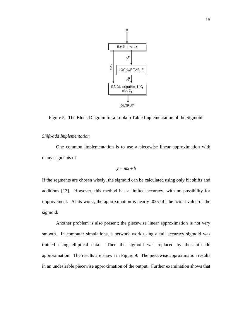
Look Up Table Implementation

The simplest implementation method is to use a lookup table. In order in to make

a lookup table, a limited operating range must be determined. Using the nearly odd

property,

)(1)( xfxf −=− ,

of the squashing function, the size of the lookup table can be decreased to half the desired

range. The non-saturation range is between -8 and 8, so the look-up table only needs

operate between 0 and 8. This requires three integer bits and all eight fractional bits to be

used as address bits. Any numbers not in that range are considered to be in saturation and

assigned an output value of 1. The resulting table has eleven address bits selecting the

eight bit fractional portion, using two kilobytes of memory. The lookup table

implementation of a sigmoid has a latency of three. This implementation could be

undesirable since available on-chip memory may be needed for weight storage.

15

Figure 5: The Block Diagram for a Lookup Table Implementation of the Sigmoid.

Shift-add Implementation

One common implementation is to use a piecewise linear approximation with

many segments of

bmxy +=

If the segments are chosen wisely, the sigmoid can be calculated using only bit shifts and

additions [13]. However, this method has a limited accuracy, with no possibility for

improvement. At its worst, the approximation is nearly .025 off the actual value of the

sigmoid.

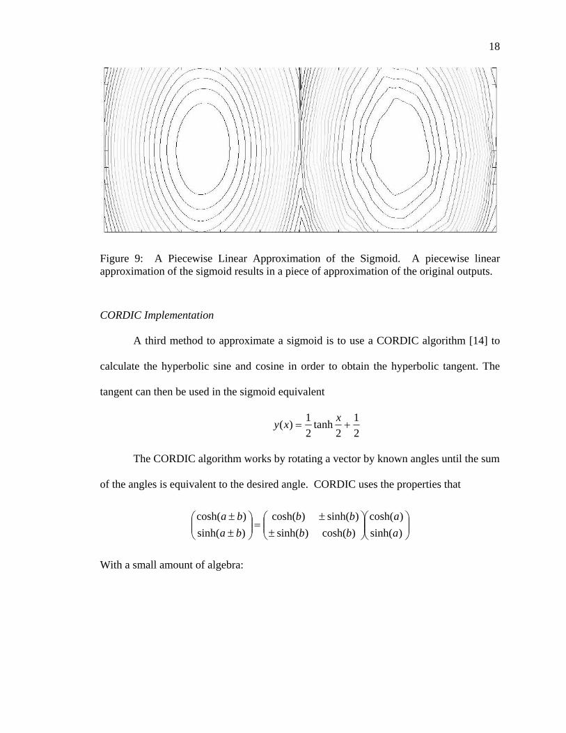
Another problem is also present; the piecewise linear approximation is not very

smooth. In computer simulations, a network work using a full accuracy sigmoid was

trained using elliptical data. Then the sigmoid was replaced by the shift-add

approximation. The results are shown in Figure 9. The piecewise approximation results

in an undesirable piecewise approximation of the output. Further examination shows that

16

training with the shift-add approach also results in piecewise outputs. The shift-add

implementation of the sigmoid has a latency of five.

Figure 6: The Block Diagram for a Shift-Add Implementation of the Sigmoid.

TABLE 1

SEGMENTS USED FOR THE SHIFT AND ADD APROXIMATION

Lower Bound Slope Constant 7.236 0 1.0 5.846 1/512 0.984375 5.147 1/256 0.97265625 4.442 1/128 0.953125 3.724 1/64 0.91796875 2.977 1/32 0.859375 2.164 1/16 0.765625 1.065 1/8 0.6328125 0.0 1/4 0.5

17

Figure 7: VHDL Approximation of Shift and Add Squashing Function. The VHDL implementation of the shift-add squash is on the left and the error is shown on the right. The shift and add approximation of the sigmoid is nearly 3% off from the actual at its worst.

Figure 8: Comparison of Shift-Add FPGA Output with Real Output. One of the known input/output relationships was used to test the FPGA implementation. The map on the left shows a comparison of the real image and that produced by the FPGA. The absolute difference of the two images is shown in the map on the right.

18

Figure 9: A Piecewise Linear Approximation of the Sigmoid. A piecewise linear approximation of the sigmoid results in a piece of approximation of the original outputs.

CORDIC Implementation

A third method to approximate a sigmoid is to use a CORDIC algorithm [14] to

calculate the hyperbolic sine and cosine in order to obtain the hyperbolic tangent. The

tangent can then be used in the sigmoid equivalent

21

2tanh

21)( +=

xxy

The CORDIC algorithm works by rotating a vector by known angles until the sum

of the angles is equivalent to the desired angle. CORDIC uses the properties that

⎟⎟⎠

⎞⎜⎜⎝

⎛⎟⎟⎠

⎞⎜⎜⎝

⎛±

±=⎟⎟

⎠

⎞⎜⎜⎝

⎛±±

)sinh()cosh(

)cosh()sinh()sinh()cosh(

)sinh()cosh(

aa

bbbb

baba

With a small amount of algebra:

19

⎟⎟⎠

⎞⎜⎜⎝

⎛⎟⎟⎠

⎞⎜⎜⎝

⎛±

±=⎟⎟

⎠

⎞⎜⎜⎝

⎛±±

)sinh()cosh(

1)tanh()tanh(1

)cosh()sinh()cosh(

aa

bb

bbaba

))sinh()tanh())(cosh(cosh()cosh( ababba ±=±

))cosh()tanh())(sinh(cosh()sinh( ababba ±=±

By starting with the hyperbolic sine and cosine of known angle a, a desired

hyperbolic sine and cosine can be calculated by applying the above equations with known

b and previously calculated cosh(b) and tanh(b). The equations can be applied repeatedly

with other known b’s until the proper sum is reached.

By choosing tanh(b) to be negative powers of 2, such as 1/2, 1/4, 1/8, etc., all the

multiplications can be executed as shifts. The cosh(b) can be found for each of the

previous. The product of the cosh(b) from all iterations is found and used as an initial

constant.

The most commonly used initial argument is zero, with the starting vector as

(1.20744 0). However, the range of the CORDIC algorithm starting at this vector is

limited to the sums of the known b’s. When using tanh(b) as only powers of 2, the radius

of convergence is slightly greater than 1.13.

This creates a problem with the sigmoid implementation. Using the almost odd

property, the desired sigmoid range is from zero to eight. Though since the argument is

divided by two, the necessary range of the hyperbolic tangent is zero to four, which is out

of the convergence range.

In order to get the necessary range to converge, the desired range is divided into

segments the same size as the standard range. In this case, two segments were used, zero

to two and two to four. Then, when a tangent needs to be found, the initial vector is

20

chosen based on the argument. If it the argument is in the first segment, the initial vector

is chosen to be the hyperbolic cosine and sine of one multiplied by the product of the

cosh(b) and the cosh(1). For the second segment, the hyperbolic cosine and sine of three

is used along with the product of the cosh(b) and cosh(3). This way, the regions of

convergence for the two segments overlap slightly and also extend beyond the desired

range. If more range is necessary, more segments can be used. If a more accurate result

is desired, more CORDIC rotations can be used.

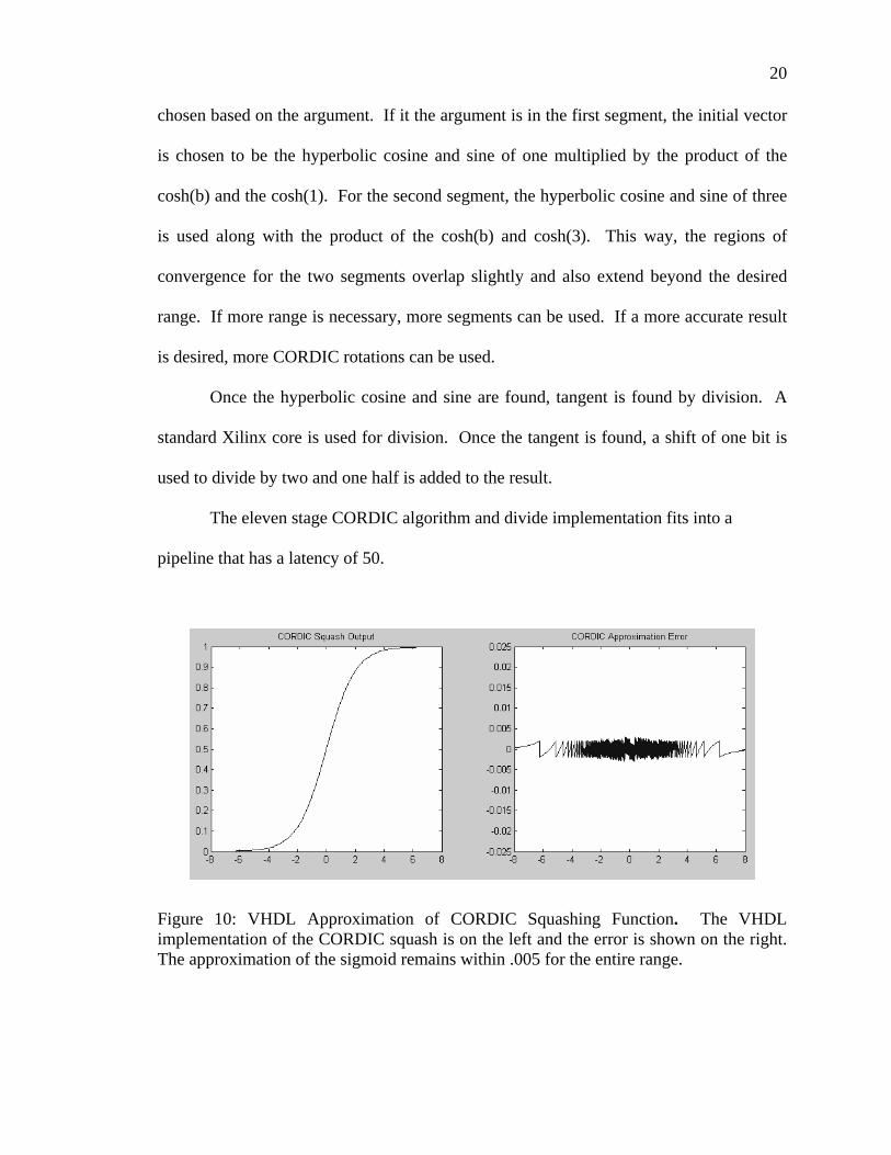
Once the hyperbolic cosine and sine are found, tangent is found by division. A

standard Xilinx core is used for division. Once the tangent is found, a shift of one bit is

used to divide by two and one half is added to the result.

The eleven stage CORDIC algorithm and divide implementation fits into a

pipeline that has a latency of 50.

Figure 10: VHDL Approximation of CORDIC Squashing Function. The VHDL implementation of the CORDIC squash is on the left and the error is shown on the right. The approximation of the sigmoid remains within .005 for the entire range.

21

TABLE 2

CORDIC INITIALIZING SEGMENTS

Segment Center Hyperbolic Cosine Hyperbolic Sine 1 1.89325 1.419043 3 12.1566 12.09648

Figure 11: The Block Diagram for a CORDIC Implementation of the Sigmoid.

22

Figure 12: Comparison of CORDIC FPGA Output and Real Output. One of the known input/output relationships was used to test the FPGA implementation. The map on the left shows a comparison of the real image and that produced by the FPGA. The absolute difference of the two images is shown in the map on the right.

Taylor Segments Approximation

The fourth approximation examined was a Taylor series about zero, though

convergence was slow. To avoid this problem, several second order segments of Taylor

series about different points are used, with a general formula of

0002

00 )(')(")( yxxyxxyxy +−∗+−∗−=

Then, given the argument, the proper offset and coefficients are chosen. The accuracy of

the approximation can be improved by increasing the number of segments used in the

approximation. This implementation uses three multipliers, three adders, three

multiplexers, and a number of comparators equivalent to the number of segments.

As with the other implementations, a pipelined version is desired. The pipeline is

shown in Figure 13. It was expected that the pipeline would have a latency of eight.

However, for multipliers on the XC2V6000 to operate at 100 MHz, a latency of two is

required to complete a computation. Since there are two stages of multipliers, the total

latency is ten.

23

TABLE 3:

TAYLOR SERIES SEGMENTS AND COEFFICIENTS

Lower Bound x0 y0” y0’ y0 7.293 0.0 0.0 0.0 1.0000000000004.771 6 0.001220703125 0.00244140625000 0.9975585937503.317 4 0.008544921875 0.01757812500000 0.9820556640632.482 2.75 0.024780273438 0.05639648437500 0.9399414062500.425 1 0.045288085938 0.19653320312500 0.7310791015630.0 0 -- 0.25000000000000 0.500000000000

Figure 13: The Block Diagram for a Taylor Series Implementation of the Sigmoid.

24

Figure 14: VHDL Approximation. The VHDL implementation of the Taylor series squash is on the left and the error is shown on the right. The approximation of the sigmoid remains within .005 for the entire range.

Figure 15: Comparison of FPGA Output with Real Output. One of the known input/output relationships was used to test the FPGA implementation. The image map on the left was produced by the FPGA and the image map on the right was produced by the original neural network.

Comparison Summary

Table 4 is a comparison of the different implementations, showing the amount of

chip assets necessary, latency and error for each implementation. The average pixel error

was found using a computer simulation holding all other calculations at maximum

accuracy and using the approximation in place of the sigmoid.

25

TABLE 4

A COMPARISON OF APPROXIMATIONS

Implementation Slices Memory Multipliers Latency Average Pixel Error

Lookup Table 1951 2kbytes 0 3 0.4015 Shift-add 2026 0 0 5 1.3281 CORDIC 3475 0 0 50 0.4279 Taylor Series 2085 0 3 10 0.4306

For our problem, fast weight access requires storage in on-chip memory and

multipliers also limit the amount of memory available. This makes memory limited and

the lookup table approach infeasible. However, given a smaller network or more

resources, a lookup table implementation would be ideal.

The shift and add implementation is small with a low latency and uses no

predefined logic for its implementation. However, it has the worst error, three times that

of any other implementation. It also has no method for improvement.

The CORDIC version has the lowest error, though is significantly larger than the

other four versions. This version also has a very long latency, which, in a four layer

network, would add 200 clock cycles versus the next slowest 40. However, error

improvement is easily done by adding more stages and can be done as long as chip area is

available.

The Taylor series approximation has the third best error of four implementations,

though is not much worse than the smallest error. The small improvement in latency that

would be gained by using the shift-add implementation is outweighed by the increase in

error and the cost of a piece-wise approximation. The desire for speed also outweighs the

small error improvement that would be gained by switching to a CORDIC

26

implementation. In the end, we are proceeding with this network implementation using a

Taylor series approximation. The actual average error resulting from the Taylor series

implementation in hardware is 1.4230 units per pixel.

27

CHAPTER FIVE

Neural Network Implementations For this problem, several different implementation structures were used. Initially

a simple design was used to test the ability of the FPGA to calculate the neural network

as well as to become comfortable with the programming environment. Next, a few

similar versions of the initial design were implemented in order to increase the speed of

the forward computation. Finally, a completely different approach was taken to achieve

the current speed up.

Serial Implementation

The first implementation performed all network calculations serially. Three on-

board memory banks were used. One of the memory banks held the network weights

with one weight per memory location. Since the inputs for the next layer are written

while the current layer inputs are being read, two banks must be used to hold layer inputs.

One multiplier and one accumulator are used to calculate the sum of products input to a

node. The inputs from one bank and the weights are used as the inputs to the multiplier.

The products are then summed by the accumulator until a node sum is completed. Then

the result of the node is squashed and the result stored in the other input bank. While

result is being squashed, the accumulator is cleared and the calculations for the next node

begin. Once a layer is complete, the newly calculated input bank is used for the

multiplier inputs while the other input bank is written over for the next layer’s inputs.

28

For the final layer, the squash is bypassed and outputs are taken directly from the

accumulator. A block diagram for the serial implementation is shown in Figure 16.

Since the serial implementation can perform one input-weight multiply per clock,

the number of clocks required is equivalent the number of weights plus the latency of the

squashing implementation. Since the number of weights is much greater than the latency,

calculation time can be considered to be approximately the number of weights. The

acoustic network contains approximately ninety-two thousand weights. This takes

approximately ninety-two thousand clocks for a forward evaluation or, at one hundred

megahertz, just under one millisecond.

Weight0Weight0

Weight1Weight1

Weight2Weight2

Multiply and AccumulateMultiply and Accumulate

Squashing FunctionSquashing Function

Weights

Outputs

Input Bank2

Input Bank2

Input Bank1

Input Bank1

MultiplexerMultiplexer

SelectSelect

Weight0Weight0

Weight1Weight1

Weight2Weight2

Multiply and AccumulateMultiply and Accumulate


Weights

Outputs

Input Bank2

Input Bank2

Input Bank1

Input Bank1


SelectSelect

Figure 16: The Block Diagram for the Serial Implementation of a Neural Network

Parallel Node Implementation

One method to speed up the implementation is to calculate more than one node at

a time. The structure for each node is identical to the serial implementation. However,

several nodes for the next layer are calculated in parallel, decreasing computation time.

29

In order to calculate multiple nodes in parallel, several weights must be accessed

at the same time. For the initial node parallel implementation, four nodes are calculated

at a time, requiring four weights per clock. To do this, four sixteen-bit weights are stored

in the sixty-four bit memory in the on board banks. Then, on each clock, four multiply

and accumulators multiply an input by four different weights and find the sum of

products for four nodes. As with the serial version, two banks are used for reading and

writing inputs, and the accumulators are cleared when the calculations for new nodes

began.

For the four node parallel version, it would seem that four squashing functions

would be needed. However, the since inputs are retrieved at a rate of one per clock from

the memory banks, they must also be written to at a rate of one per clock. To achieve

this, while one node-sum begins a squash, the other three are stored in registers. Since

the squashing function is pipelined, the other three are squashed in order, directly

following the first. This allows the four node outputs to leave the pipeline serially where

they are written directly to an input bank.

At most, this method could speed up the forward computation time of a neural

network by a factor of four. However, not all layers have node multiples of four, so a

few of the parallel node calculations are wasted calculating nonexistent nodes. The

weights for the nonexistent nodes are filled with zeros. For the approximately ninety-two

thousand weight neural network, the time for one forward evaluation at one hundred

megahertz is roughly .25 milliseconds. A block diagram for the parallel node

implementation for four nodes is shown in Figure 17.

30

Weight0AWeight0A

Weight1AWeight1A

Weight2AWeight2A

Multiply and Accumulate



Weights A

Outputs

Input Bank2

Input Bank2

Input Bank1

Input Bank1


SelectSelect

Weight0BWeight0B

Weight1BWeight1B

Weight2BWeight2B



Weights B

Weight0CWeight0C

Weight1CWeight1C

Weight2CWeight2C



Weights C

Weight0DWeight0D

Weight1DWeight1D

Weight2DWeight2D



Weights D

RegisterRegister RegisterRegister RegisterRegister RegisterRegister

Weight0AWeight0A

Weight1AWeight1A

Weight2AWeight2A




Weights A

Outputs

Input Bank2

Input Bank2

Input Bank1

Input Bank1


SelectSelect

Weight0BWeight0B

Weight1BWeight1B

Weight2BWeight2B



Weights B

Weight0CWeight0C

Weight1CWeight1C

Weight2CWeight2C



Weights C

Weight0DWeight0D

Weight1DWeight1D

Weight2DWeight2D



Weights D

RegisterRegister RegisterRegister RegisterRegister RegisterRegister

Figure 17: The Parallel Node Implementation with Four Parallel Nodes.

A variation on this method was also implemented in order to achieve even greater

speed up. The SRC-6e has six on-board memory banks. The input storage requires the

use of two of the banks, leaving four banks of weight storage. Since each bank can hold

four weights per memory location, a maximum of sixteen weights can be retrieved per

clock cycle. This limits this implementation a maximum sixteen parallel multiplications.

If the four node parallel implementation is simply extended out to sixteen, many

multiplies are wasted. To calculate a layer of fifty nodes, for example, in the last set of

sixteen nodes, the final fourteen nodes are unnecessary. In order to avoid this waste, only

four nodes are calculated at in parallel; however, four multiplications per node are also

computed, using all sixteen available weights. Then the four products are summed and

stored in an accumulator, allowing nodes to be calculated four times as quickly. Then the

number of non-existent node calculations at the end of a layer is equivalent to that of the

previous implementation.

31

In order to use four weights per node, four inputs must also be used per clock.

Since sixteen bit inputs are stored in a sixty-four bit bank, four are stored in each memory

address and are accessible every clock. Four squashed outputs must also be stored at the

same time for use as future inputs. Instead of shifting data into one squashing function,

four squashing functions are implemented in parallel. Then after node multiplications

and accumulations are completed, all four nodes are squashed and the results are

available at the same time for storage.

This method is nearly sixteen times faster than the serial implementation. At one

hundred megahertz, the time for a forward calculation of the ninety-two thousand weight

network is approximately sixty microseconds. A simplified block diagram for the

implementation with sixteen multiplications in parallel is shown in Figure 18.

Weights0-3AWeights0-3A

Weight4-7AWeight4-7A


4 Multiplies4 Multiplies

SquashSquash

Weights A

Outputs

Input Bank2

Input Bank2

Input Bank1

Input Bank1


SelectSelect Weights B Weights C Weights D

Sum and AccumulateSum and

Accumulate

Weights0-3BWeights0-3B

Weight4-7BWeight4-7B


Weights0-3CWeights0-3C

Weight4-7CWeight4-7C


Weights0-3DWeights0-3D

Weight4-7DWeight4-7D


4 Multiplies4 Multiplies 4 Multiplies4 Multiplies 4 Multiplies4 Multiplies


AccumulateSum and

AccumulateSum and

AccumulateSum and

AccumulateSum and

Accumulate

SquashSquash SquashSquash SquashSquash

Outputs Outputs Outputs

Weights0-3AWeights0-3A



4 Multiplies4 Multiplies

SquashSquash

Weights A

Outputs

Input Bank2

Input Bank2

Input Bank1

Input Bank1


SelectSelect Weights B Weights C Weights D


Accumulate

Weights0-3BWeights0-3B



Weights0-3CWeights0-3C



Weights0-3DWeights0-3D



4 Multiplies4 Multiplies 4 Multiplies4 Multiplies 4 Multiplies4 Multiplies


AccumulateSum and

AccumulateSum and

AccumulateSum and

AccumulateSum and

Accumulate

SquashSquash SquashSquash SquashSquash

Outputs Outputs Outputs

Figure 18: Parallel Node Implementation with Sixteen Multiplies

32

Parallel Input Implementation

By storing weights and inputs in on-chip BRAM, many more weights can be

accessed at a time as well as an entire layer of inputs. This allows many calculations to

be performed in parallel, giving a significant speed increase over a serial computer.

The parallel input implementation performs all the multiplications for the

calculation of one node at the same time. The previous layers outputs are multiplied by

the corresponding weights for the current node. While the products are being summed,

the next node’s weights are multiplied by the same set of outputs, creating an efficient

pipeline. However, since all the node outputs are required for calculations in the next

layer, the pipeline must wait several clocks for the previous layer to finish before

continuing with the next.

In order to simplify the implementation of the network, all layers are considered

to be the same size as the largest, in this case, 70 nodes. Weights beyond the range of

small layers are set to zero. The number of nodes calculated is controlled in order to

minimize the amount of filler zero weights used. A block diagram of the node parallel

calculation is shown in Figure 19. Pseudo code for control is shown below:

Multiply all inputs by all current weights Sum all the products Squash the sum Save the squashed sum in output memory Increment weight counter Increment output counter If output counter equals number of nodes on next layer reset the output counter write output memory over input memory increment layer counter

33

This design takes 1465 clocks to complete one network evaluation or slightly less

than fifteen microseconds. This allows the network to be evaluated more than sixty

thousand times per second.

Weight0Weight0 Weight70

Weight70

Inputs/Node Memory

Inputs/Node Memory

71 Multiplies and Pipelined Sum71 Multiplies and Pipelined Sum

Squash FunctionSquash Function

Inputs Weights

Outputs


Weight70


Weight70

7171Weight0

Weight0 Weight70Weight70

Inputs/Node Memory

Inputs/Node Memory

71 Multiplies and Pipelined Sum71 Multiplies and Pipelined Sum

Squash FunctionSquash Function

Inputs Weights

Outputs


Weight70


Weight70

7171

Figure 19: A Simplified Block Diagram of a Node Parallel Implementation.

Conclusions on Neural Network Implementations

This example has shown that a hardware neural network can reasonably

approximate a continuous neural network using limited accuracy for weights as well as

an approximation of the squashing function. However, it must be noted that neural

networks are approximations of an actual system. By approximating an approximation,

needless noise is added. This problem could be avoided by training on a hardware

implementation; in other words, set the weights by training with the limited accuracy as

well as with the approximated squashing function.

The training could be completed using a random initialization of weights or by

using the pre-trained network weights as a starting point. In either case, the squashing

34

function used could be chosen based more on speed of calculation rather than on how

close the approximation is to the sigmoid. The shift-add version would probably be used

due its size and speed. The shift-add implementation is only capable of piecewise linear

approximations, though given the size of network, the number of linear segments is likely

adequate.

The three different versions of neural networks could be useful in different

situations. The serial implementation will fit into a small FPGA with only a few input

pins for the three memory banks used. Then a circuit board could be created with a few

RAM blocks and the FPGA. Inputs could be retrieved from analog to digital converters

or other sources and outputs used by a computer or other segments of circuitry.

The parallel node implementation could be tailored for a problem that needs more

speed than the serial implementation provides, though still needs a reasonably small

FPGA. More connections would have to be made to access the greater number of

memory banks, though outputs would be available four or sixteen times as quickly with

four available at a time.

The parallel input implementation is useful in cases where maximum speed is

necessary, such as in the real-time particle swarm inversion. For the forward

computation, given a chip with enough pins, all inputs could be clocked in at the same

time and used directly as the first layer inputs. Outputs, however, are still required to be

received sequentially, as they are calculated sequentially.

35

CHAPTER SIX

Particle Swarm Implementation

The particle swarm update equations consist of simple multiplications and

additions, easily implemented on a XC2V6000. Setting the bias coefficients to powers of

two and using shifts in place of multipliers further simplifies the implementation. The

computation time for a hardware particle swarm optimization is solely dependent on the

computation time of the fitness function. The position and velocity of one agent can be

updated while the fitness of another agent is being calculated. Since the fitness function

takes orders of magnitude longer to calculate, the update hardware will be inactive for a

large majority of the time.

The more complicated part of the update equations is the randomness associated

with the velocity update. For this implementation, we examined three different methods

for implementing the randomness. For comparison, a standard particle swarm was run on

a conventional computer. The average error over one hundred trials between desired

output and that calculated using the found input was 1.9385 units per pixel.

Deterministic Particle Swarm

The first method to implement randomness was simply to ignore it. Randomness

was previously successfully removed to prove the stability of the algorithm [15].

Removing randomness would simplify the implementation of the particle swarm update

equations. In order to estimate the effectiveness, randomness was removed from particle

swarm on a conventional computer. The bias coefficients were also decreased so that the

36

average bias would be the same. Both the random and the deterministic particle swarms

were run for ten thousand iterations for thirty searches. The global best fitness was

plotted for each run as well as the average of all swarms. The plot is shown in Figure 20.

For our problem, it initially appeared that including the randomness would significantly

increase the success of the swarm.

Figure 20: Particle Swarm with and without Randomness. Random and deterministic particle swarms were run for ten thousand iterations thirty times. The crosses are the global best results from the deterministic particle swarm and the top line the average. The circles are the global best results from the particle swarm with randomness and the bottom line the average. The randomness significantly improves the result of particle swarm.

The deterministic particle swarm update equations lend themselves to a parallel

hardware implementation since the velocity and position can be calculated at the same

time. The update equations are implemented in a pipeline and one dimension can be

updated on every clock cycle. The block diagram for the hardware implementation is

37

shown in Figure 21. The average error over one hundred trials between the desired

output and that calculated using the found input was 2.3587 units per pixel.

Figure 21: Deterministic Particle Swarm Block Diagram.

Randomization

In order to implement randomness, a function is implemented that generated two

pseudorandom numbers per clock. Two stages are added to the update pipeline to

multiply the personal bias and global bias by the generated numbers.

Linear Feedback Shift Register

One method of generating pseudorandom numbers is to use a linear feedback shift

register. This method is typically used in testing digital logic designs. The Fibonacci

implementation begins with an initial seed value loaded into a shift register. The value is

then shifted one bit with the carry in bit determined by a logical combination of the bits

in the previous value [16].

Prior to implementation, the quality of the randomness of the method was tested

in computer simulations. Ideally, the probability of an output of a uniform random would

XnDimk VnDimk PnDimk Gk VmaxkXmaxk Xmink

X+V

Compare

New XnDimk

P-X G-X

V+1/8(P-X)+1/16(G-X)

Xmink Xmaxk VnDimk Vmaxk

Vmaxk

Compare

New VnDimk

New XnDimk

38

be equal for all values with in the specified range. Figure 22 shows the histogram of ten

thousand outputs from an LFSR as well as that of the uniform random number generator

from a computer simulation. The LFSR result appears to slightly favor values in the

extremes, while the computer simulation generator appears to be uniform throughout. At

this point, the LFSR appears to be a suitable uniform random number generator.

The second requirement to be an acceptable uniform random number generator is

that one output should not be related to other outputs. A good method to verify this is

that the frequencies present in a stream of unrelated outputs is uniform. Figure 23 shows

the frequencies present in the LFSR and in the computer simulation generator as well as

short segment of the stream. As expected, the computer simulation generator has all

frequencies present at fairly equal strengths. The LFSR, however, has predominately low

frequencies, indicating that adjacent outputs are highly related to each other. This is

apparent from looking at the output streams. The computer simulation generator varies

greatly between samples while the LFSR output follows a curved pattern. This indicates

that the linear feedback shift register does not make a very good uniform random number

generator.

Even though it is not a perfect random number generator, the linear feedback shift

register was implemented into the particle swarm. For sixteen bits of randomness, the

last sixteen bits are taken from a twenty-one bit LFSR. The average error over one

hundred trials between the desired output and that calculated using the found input was

2.3522 units per pixel.

39

Figure 22: Histograms for a LFSR Implementation and a Uniform Random Variable.

Figure 23: Output Streams and Frequency Spectra f or a LFSR Implementation and a Uniform Random Variable.

40

Squared Decimal Implementation

A second method of generating pseudorandom numbers was based on the pi to the

fifth method. It is possible to create a stream of apparently random numbers by adding a

decimal number to pi and then taking the sum to the fifth power. The fractional portion

of the result is the pseudorandom number and used as the next number added to pi. This

method is not specific to pi or to the fifth power. The hardware implementation uses a

squared power and a one followed seventeen randomly assigned fractional bits in place of

pi.

As with the linear feedback shift register, the quality of the randomness was tested

in computer simulations and compared with that of the computer simulation uniform

random variable generator. From the histogram shown in Figure 24, the squared decimal

random generator is not uniform in nature and appears to have a tendency towards

smaller numbers. In this aspect, it is worse than the linear feedback shift register

implementation. However, in the frequency spectrum shown in Figure 25, the squared

decimal implementation is more uniform. This manifests itself in the output stream,

which contains no obvious patterns. In this aspect the squared decimal implementation is

closer to being more random between samples than the LFSR.

As with the LFSR, the squared decimal implementation was generated in

hardware and used in the particle swarm search. The average error over one hundred

trials between the desired output and that calculated using the found input was 2.3694

units per pixel.

41

Figure 24: Histograms for a Squared Decimal Implementation and a Uniform Random Variable.

Figure 25: Output Streams and Frequency Spectra f or a Squared Decimal Implementation and a Uniform Random Variable.

42

Particle Swarm Randomness Results

When searching for a known achievable set, all three methods of particle swarm

implementation produced approximately the same levels of output error, making the

deterministic method most desirable. In actuality, the deterministic method does

introduce some randomness due to truncation during the shifting of biases. It was also

noted that none of the implementation methods were as accurate as the conventional

computer average error of 1.9385 units per pixel.

In order to account for this increase, it was noted that the hardware

implementation was not searching using an identical network to the computer. Therefore,

a more accurate comparison can be made using output from the hardware neural network

given the found inputs. Comparing to the hardware output, the average pixel error for the

deterministic method was 1.8055 units per pixel, actually better than the conventional

swarm. The average pixel error of 1.4230 between the computer network outputs and

hardware network outputs combined with the search error gave rise to the overall higher

error.

The average pixel error between the computer network outputs and the acoustic

model outputs that it is mimicking is 4.5801 units per pixel. With this level of error

already in the system, the extra .5 units of error caused by the network and particle swarm

translation to hardware were deemed to be insignificant.

Conclusions on Particle Swarm Implementation

The output from the hardware particle swarm inversion has an average pixel

difference of 2.5387 from a known achievable desired output or an average difference of

43

1.53%. This low error implies that the particle swarm inversion will be able to find a set

of inputs that produces outputs closest or near the closest to a desired output set.

Figure 26 and Figure 27 show two sets of outputs from inputs found for the

maximization of a specific area as well as the specified area. All other areas were

ignored for calculation of fitness. Localized maximization is equivalent to attempting to

find infinite ensonification, which, of course, is outside the achievable set. It is evident

from the figures that the particle swarm optimization found a set of inputs which

maximizes the local area and ignores the rest of the figure.

The time to complete the same one hundred thousand iteration particle swarm

optimization on a conventional computer is nearly two minutes. At one hundred

megahertz, the two-chip hardware implementation takes under 1.8 seconds to complete

and is approximately sixty-five times faster.

Figure 26: Particle Swarm Results Maximizing a Specified Area. The white area in the image on the right shows the desired maximization area. The image on the left shows the outputs from the solution found by the particle swarm.

44

Figure 27: Particle Swarm Results Maximizing a Specified Area. The white area in the image on the right shows the desired maximization area. The image on the left shows the outputs from the solution found by the particle swarm.

45

CHAPTER SEVEN

Algorithm Speedup through FPGA Implementation

High-end consumer computers have processors operating at speeds greater

than three gigahertz and cost less than a few thousand dollars. FPGAs, however,

typically run no faster than a few hundred megahertz and can cost several thousand

dollars per chip. For certain algorithms the time saved by the ability to perform

computations in parallel is lost from the slower clock speed of the FPGA. Other factors

that determine algorithm calculation time include the ability for an algorithm to be

pipelined and the speed at which memory can be accessed.

Parallel-able

Algorithms which perform many independent calculations are typically prime

candidates for FPGA implementation. The calculations can be performed in parallel by

the FPGA, whereas in a conventional computer they are performed serially. The increase

in algebraic calculations per clock can provide a large speedup over a serial computer

operating at the same rate. For the neural network example, many thousands of

independent calculations are performed, making it a strong candidate for hardware

implementation. On the output layer, around seventy thousand multiplications could be

preformed in parallel, given the appropriate hardware.

The maximum speedup for an algorithm can be found by dividing the total

number of computations by the length of the largest dependent set or the largest set of

computations that cannot be performed in parallel. Speedup is considered to be the

46

number of clocks required if one calculation is performed at a time divided by the

number of clocks actually used.

The largest dependent set in a neural network is directly related to the number of

layers. For each layer, a multiply, a sum, and a squash must be performed before

calculations for the next layer can begin. A multiplication requires two clock cycles and

using an ideal lookup table, a squash requires one clock cycle. Only a limited number of

terms can be summed in a clock cycle, so the number of clock cycles required is

logarithmically related to the number of terms in the layer. For the example neural

network and hardware, only five terms can be summed per clock to achieve timing.

Therefore, the sum for each layer takes three clock cycles to complete. Each layer needs

six clock cycles to complete, except for the output layer which only needs five. With

three hidden layer calculations and one output layer calculation, the longest set of

dependent calculations is twenty-three.

The required calculations are approximately ninety thousand multiplies, ninety

thousand additions, and one hundred and sixty squashes. This combines for a total

number of serial clocks of about one hundred eighty thousand. This results in a

maximum speed up from parallel-ability of about eight thousand.

However, the maximum speedup is not possible due to hardware constraints, so

the real speedup due to parallel-ability is considered to be the total number of calculations

divided by the longest length of dependent calculations multiplied by the number of times

the calculations are repeated. For the first three layers, the longest dependent set is

twenty-five and this repeated one hundred sixty times. For the final layer, the longest

47

dependent set is ten and is repeated one thousand two hundred times. This gives an

actual speedup due to parallel-ability of about eleven.

The particle swarm update is an example of another algorithm which can achieve

speedup through parallel-ability. With the above example, all twenty-seven dimensions

could be updated simultaneously. Internal to each update, an additional speed up of three

is achievable through performing calculations in parallel. This gives a total speed up of

eighty-one.

The CORDIC algorithm, however, does not achieve much gain from parallel-

ability. The CORDIC rotation calculations are all related and require a serial

implementation. With each rotation dependent on the previous, the only parallel gain is

from the three algebraic computations for a rotation. The Taylor series and shift-add

approximations are two other examples in which limited gain is made from parallel-

ability.

Pipeline-able

Even if an algorithm does not have many unrelated calculations, it is still possible

for an implementation to be advantageous if the algorithm is pipeline-able. The

maximum speedup achievable from pipelining is the length of the longest set of

calculations that cannot be performed in parallel. The total maximum speedup is the

speedup from parallel-ability multiplied by the speed up from pipelining. This gives

maximum speedup equal to the number of calculations in an algorithm.

The CORDIC algorithm, for example, is pipeline-able, and this is especially

useful if many stages of the algorithm are used. In the pipeline, many calculations are

performed at the same time; however, each is for a different input. Then, total speedup is

48

not only the three calculations performed in parallel, but also the length of the pipeline

used. A ten stage CORDIC algorithm would perform three calculations in parallel

multiplied by ten stages in the pipeline, or thirty calculations per clock. This speedup

makes a one hundred megahertz FPGA competitive with a three gigahertz serial

computer operating at one calculation per clock.

This maximum speed up cannot actually be achieved. However, it is approached

as the number of the CORDIC computations needed to be performed increases. If only a

few computations are required, the full speedup effect is not appreciated due to the extra

clocks from the latency when waiting for the last computation to be completed. The real

amount of speed up is

⎟⎠⎞

⎜⎝⎛

−+=

1LNNSS ma

Where Sa is the actual speedup, Sm is the maximum speedup, N is the number of

computations to be performed and L is the latency of the pipeline. In the pipelined

CORDIC algorithm, if only one computation is required and the pipeline is ten stages,

then the actual speedup is only three. As expected, this is the same as that found when

examining parallel-ability.

Some algorithms, such as the neural network, are unable to be fully pipelined due

to hardware limitations. Given enough hardware, a neural network would be able to be

pipelined to perform all multiplications, additions and sigmoid calculations

simultaneously. In the case of the example neural network, the gain would be the

combination of the gains for the multiplications, additions and squashing functions, or for

a total of around one hundred.

49

However, it is not possible to perform all calculations at one time and hardware

must be reused, making it impossible to achieve one evaluation per clock. A pipeline

gain is still achieved with the calculation of individual nodes. The squashed sum of each

node for a layer can be treated as different computations and a pipeline made evaluating

one node per clock.

For each layer, the above speed up equation holds with N set to the number of

nodes and L set to the latency of calculating one node. The maximum speedup changes

from layer to layer due to the different number of multiplies between layers as well as the

latency that is required because one layer must finish before another begins. The

average speedup per node due to pipeline-ability is approximately eleven. The pipeline

speedup combined with the parallel speedup gives a total speed up of one hundred and

twenty-one. This is equivalent to the one hundred and eighty thousand serial clocks

needed divided by the clocks necessary to complete one forward evaluation.

Memory Transfer

Another important factor in considering the usefulness of an FPGA

implementation is the memory transfer that occurs. To use an FPGA algorithm, the

microprocessors in the SRC-6e must first retrieve data from main memory and then load

it into the on-board memory banks. If the algorithm was performed directly in the

microprocessors, the data is only needed to be retrieved from memory, at which point it

can remain in cache to be reused. The extra time of transferring data to and from the on-

board memory banks can make a hardware implementation slower than that in a

microprocessor.

50

The CORDIC example is one case. With a ten stage CORDIC pipeline, the

speedup is thirty. This makes a one hundred megahertz hardware implementation as fast

as a three gigahertz serial processor. However, if data is stored and retrieved in the on-

board memory with a one hundred megahertz processor, an extra two clocks per

calculation is needed, taking the time per calculation from one clock to three. This is a

slowdown by three, making the net speedup only ten. This makes the CORDIC

implementation only competitive with a one gigahertz serial computer. For any fully

pipelined implementation, the speedup decreases by three.

The neural network speed is impacted less by data transfer. This is, however,

partly due to the large number of clocks used to calculate a forward evaluation. Only

twenty-seven inputs are transferred to the on-board memory and twelve hundred outputs

are transferred out. This increases the clocks used from 1465 to 2837, or a slowdown of

about 1.93. This takes the net speedup from 123 to about 64.

Particle swarm is hurt the least by data transfer. It takes about one hundred and

fifty million clocks to complete. The only data transferred is the twelve hundred desired

outputs and the twenty seven found inputs. This is a slowdown of well under one percent

and can be considered negligible.

Speed Ratio

In the end, all three of the above factors must be considered when considering

whether or not to implement an algorithm in hardware. Typically rough estimates of

speedups for parallel-ability and pipeline-ability and the slowdown from data transfer are

accurate enough to determine whether an algorithm will be more efficient in a hardware

implementation or in a faster dedicated serial processor. If estimates are not accurate

51

enough to confidently say which will be faster, programming both and comparing actual

times is probably unnecessary. Given the choice between a hardware implementation

and a possibly slightly slower microprocessor program, the extra cost saved by using the

microprocessor will likely balance any speed gain.

Conclusions

For the neural network implementation, several approximations were made in

both the data representation and in algorithm calculations in order to accommodate the

hardware limitations of the FPGA as well as to decrease calculation time. The error

added by the translation to a sixteen-bit fixed point representation proved to be

insignificant. Error from approximating the squashing function also showed to be

insignificant. After examining various implementations, a Taylor Series approximation

was used for the final network implementation.

Once approximations were proven to be feasible, various possibilities of network

implementations were examined. The parallel input network implementation was able to

achieve significant speedup through both parallel-ability and pipeline-ability; therefore,

this implementation was used for the particle swarm inversion.

The particle swarm inversion was able to achieve speedup through parallel-

ability, since its calculations could be performed during fitness evaluations. Randomness

was removed from the particle swarm update equations since it added complexity to the

implementation and minimal improvement to the results. The overall speedup of particle

swarm inversion of neural networks was enough to take the algorithm calculation time

from several minutes on a conventional computer to less than a few seconds.

52

APPENDICES

53

APPENDIX A

Parallel Input Network and Swarm Code

Main.c

#include <sys/types.h> #include <stdio.h> #include <stdlib.h> #include <libmap.h> #include <math.h> void swarm(); int main() { /*these are all the weights weights are stored in 16 bit fixed point with 4 weights per 64 bit int Fixed point for input layer is one sign bit followed by 15 fractional bits S .XXX XXXX XXXX XXXX Fixed point for middle layers is one sign bit followed by 7 integer bits and 8 fractional bits S XXX XXXX.XXXX XXXX Fixed point for output layers is one sign bit followed by 10 integer bits and 5 fractional bits S XXX XXXX XXX.X XXXX*/ uint64_t weights[24480] = { 0xfae3f80000080891, 0x0002ea04fffcff4d, 0xff9b06be0a34f634, 0xf7f309590b59ff97, 0x1918137b0e4b0966, 0x0ef20405fdc2f099, 0xdff2e041cb566079, 0x0000000000000000, 0x0000000000000000, 0x0000000000000000, //not all numbers are shown to reduced code length 0xec6cf33bfdb2fe01, 0x002a0171fe100143, 0xfea904e4006efc26, 0x002e008501d70074, 0x01f7ff82ffde000f, 0xf5b80316d9950000};

54

/*This is the maximum limit of search space, 16 bits fixed point Sign bit followed by 14 integer bits and 1 fractional bit S XXX XXXX XXXX XXX.X*/

uint64_t xMax[27] = { 364, 350, 12514, //not all numbers are shown to reduced code length 3044, 3042}; /*This is the minimum limit of search space, 16 bits fixed point

Sign bit followed by 14 integer bits and 1 fractional bit S XXX XXXX XXXX XXX.X*/

uint64_t xMin[27] = { 92, 92, 5152, //not all numbers are shown to reduced code length 2972, 2980}; /*This is the maximum velocity of particles, 16 bits fixed point

Sign bit followed by 14 integer bits and 1 fractional bit S XXX XXXX XXXX XXX.X*/

uint64_t vMax[27] = { 54, 52, //not all numbers are shown to reduced code length 14, 12};

/*This is the starting locations of 10 search agents. 16 bits fixed point. Sign bit followed by 14 integer bits and 1 fractional bit S XXX XXXX XXXX XXX.X*/

uint64_t psuedorandx[270] = { 364, 350, //not all numbers are shown to reduced code length 2992, 2987};

/*This is the starting velocities of ten search agents, 16 bits fixed point Sign bit followed by 14 integer bits and 1 fractional bit S XXX XXXX XXXX XXX.X*/

uint64_t psuedorandv[270] ={

55

65534, 65534, //not all numbers are shown to reduced code length 6, 65534}; /*variable allocation, uses discussed further later*/ uint64_t *WEIGHTS; uint64_t *Agents; uint64_t *limits; uint64_t *desired; uint64_t *bestout; double starttime, endtime, cumetime; //time variables extern double second(); //time variables int knownouts[1200]; int mapnum = 0; int i,n,j; int x1,y1,x2,y2; int answer; FILE *knownfile; //allocate the map map_allocate(1); /*make space in memory for variables*/ WEIGHTS = (uint64_t *)Cache_Aligned_Allocate(24480 * 8); Agents = (uint64_t *)Cache_Aligned_Allocate(272 * 8); limits = (uint64_t *)Cache_Aligned_Allocate(28 * 8); desired = (uint64_t *)Cache_Aligned_Allocate(1200 * 8); bestout = (uint64_t *)Cache_Aligned_Allocate(28 * 8);

/*assign the weights to aligned memory for transfer to chip banks*/ for (i=0; i<24480; i++) { WEIGHTS[i] = weights[i]; } /*This variable is stored after the limits and it is a flag that

controls the loading of weights. 1 is load weights on function call*/ limits[27] = 1;

/*A call to the chip, the only purpose of this call is to load the weights*/ swarm(WEIGHTS, Agents, limits, desired, bestout, mapnum);

56

/*This variable is stored after the limits and it is a flag that controls the loading of weights. 0 does not load weights*/ limits[27] = 0;

/*this puts the xMax, xMin, and vMax 16 bit variables into a 64 bit variable to simplfy transfers to chip*/

uint64_t temp1,temp2,temp3; for(i=0; i<27; i++) { temp1 = xMax[i] << 32; temp2 = xMin[i] << 16; temp3 = vMax[i]; limits[i] = temp1 + temp2 + temp3; } /*this puts the starting velocity and position 16 bit variables into a 64 bit variable to simplfy transfers to chip*/ for(i=0; i<10; i++) { for(j=0; j<27; j++) { temp1 = psuedorandv[j+27*i] << 16; temp2 = psuedorandx[j+27*i]; Agents[j*10+i]= temp1 + temp2; } } /*Query user to determine type of search desired or to quit*/ answer = 4; while(answer !=1 && answer != 2 && answer !=3 ) { printf("Would like to match an output from the file knownouts.txt or maximize a rectangle?\n"); printf("Type 1 for known set or 2 for rectangle or 3 to quit:"); scanf("%d",&answer); } /*loop to keep doing multiple searches*/ while(answer !=3) {

/*To maximize(get as close to 0 as possible) the ensonification in a specified rectangle*/

if(answer == 2) { x1=100; x2=100;

57

y1=100; y2=100; printf("Type in corners of desired square(1<=X1<=X2<=15, 1<=Y1<=Y2<=80):\n"); while(x1>15 || x1<1) { printf("X1?:"); scanf("%d",&x1); } while(x2>15 || x2<x1) { printf("X2?:"); scanf("%d",&x2); } while(y1>80 || y1<1) { printf("Y1?:"); scanf("%d",&y1); } while(y2>80 || y2<y1) { printf("Y2?:"); scanf("%d",&y2); }

/*These loops make the desired outputs for the fitness function, with don't care being 33568 knownouts is the desired output used by the fitness function. Note that it is a 64 bit number. The fitness function uses 15 bit numbers with a sign. Since all outputs are negative, the sign bit can be treated as a normal bit and then using 65536 can be treated as zero.*/

for(i=0;i<1200;i++) { knownouts[i]=33568; } for(i=x1-1;i<x2;i++) { for(j=y1-1;j<y2;j++) { knownouts[i*80+j]=65536; } }

58

} /*A known set of outputs is stored in knownouts.txt. If this option is chosen, the set is loaded into knownouts, the desired result of fitness function. Outputs are 16 bits with 1 sign bit followed by 10 integer bits and 5 fractional bits S XXX XXXX XXX.X XXXX*/

else { knownfile = fopen("knownouts.txt","r"); for(i=0; i<1200; i++) { fscanf(knownfile,"%d",&knownouts[i]); } fclose(knownfile); } /*put the desired outputs into a variable for transfer to the chip*/ for(i=0; i<1200; i++) { desired[i] = knownouts[i]; } /*record starting time*/ starttime = second(); /*Call the PSO with appropriate variables*/ swarm(WEIGHTS, Agents, limits, desired, bestout, mapnum); /*record end time and display total calculation time*/ endtime = second(); cumetime = endtime-starttime; printf("%f seconds\n",cumetime);

/*best out is the set of inputs found the most accurately matched the desired output. The decimal value is displayed here. It is a sign bit followed by 14 integer bits

and one fractional bit. S XXX XXXX XXXX XXX.X*/ for(i=0; i<27; i++) { float temp = bestout[i]; temp = temp/2; printf("%f\n",temp); }

59

/*Query user to determine type of search desired or to quit*/

answer = 4; while(answer !=1 && answer != 2 && answer !=3 ) { printf("Would like to match an output from the file knownouts.txt or maximize a rectangle?\n"); printf("Type 1 for known set or 2 for rectangle or 3 to quit:"); scanf("%d",&answer); } }

/*uncomment this portion of code and comment above to calculate several known outs stored in knownouts.txt*/

/*knownfile = fopen("knownouts.txt","r"); for(j=0; j<100; j++) { for(i=0; i<1200; i++) { fscanf(knownfile,"%d",&knownouts[i]); desired[i] = knownouts[i]; } swarm(WEIGHTS, Agents, limits, desired, bestout, mapnum); //******************************************************* // best is the found global best //******************************************************* for(i=0; i<27; i++) { float temp = bestout[i]; temp = temp/2; printf("%f\n",temp); } } fclose(knownfile);*/ /*free the map*/ map_free(1); /*we're outta here*/ exit(0); }

60

APPENDIX B


Makefile

# ---------------------------------- # User defines FILES, MAPFILES, and BIN here # ---------------------------------- FILES = main.c MAPFILES = swarm.mc fitness.mc PRIMARY = swarm.mc SECONDARY = fitness.mc CHIP2 = fitness.mc BIN = swarm # ----------------------------------- # User defined macros info supplied here # ----------------------------------- MACROS = my_macro/squash.vhd \ my_macro/moveit.vhd MY_BLKBOX = my_macro/blkbox.v MY_NGO_DIR = my_macro MY_INFO = my_macro/macros.inf # ----------------------------------- # User supplied MCC and MFTN flags # ----------------------------------- MY_MCCFLAGS = -v MY_MFTNFLAGS = -v # ----------------------------------- # User supplied flags for C & Fortran compilers # ----------------------------------- CC = icc # icc for Intel cc for Gnu FC = ifort # ifort for Intel f77 for Gnu LD = ifort # ifort for Intel cc for Gnu

61

MY_CFLAGS = MY_FFLAGS = # ----------------------------------- # No modifications are required below # ----------------------------------- MAKIN ?= $(MC_ROOT)/opt/srcci/comp/lib/AppRules.make include $(MAKIN)

62

APPENDIX C


Swarm.mc

#include "libmap.h" void swarm(int64_t WEIGHTDATA[], int64_t AGENTDATA[], int64_t LIMITDATA[], int64_t DESIREDATA[], int64_t BESTOUT[], int mapno) { /*allocates Banks to be used by both chips*/ OBM_BANK_A(WEIGHTS, int64_t, MAX_OBM_SIZE) OBM_BANK_B(AGENTS, int64_t, MAX_OBM_SIZE) OBM_BANK_C(GLOBAL, int64_t, MAX_OBM_SIZE) OBM_BANK_D(DESIRED, int64_t, MAX_OBM_SIZE) OBM_BANK_E(G, int64_t, MAX_OBM_SIZE) OBM_BANK_F(FL, int64_t, MAX_OBM_SIZE) /*variable declerations*/ int i,j,k, wAgent; short tempA1,tempA2,tempA3,tempA4; short tempG1,tempG2,tempG3,tempG4; uint64_t error; uint64_t X[270]; uint64_t V[270]; uint64_t P[270]; uint64_t tempX, tempV; uint64_t PB[10]; uint64_t GB; uint64_t MAX_X[27]; uint64_t MIN_X[27]; uint64_t MAX_V[27]; uint64_t value_00; uint64_t value_01; uint64_t value_02;

63

uint64_t value_03; uint64_t value_04; uint64_t value_05; uint64_t value_06; uint64_t value_07; uint64_t value_08; uint64_t value_09; uint64_t value_10; uint64_t value_11; uint64_t value_12; uint64_t value_13; uint64_t value_14; uint64_t value_15; uint64_t value_16; uint64_t value_17; uint64_t value_18; uint64_t value_19; uint64_t value_20; uint64_t value_21; uint64_t value_22; uint64_t value_23; uint64_t value_24; uint64_t value_25; uint64_t value_26; uint64_t temp_00; uint64_t temp_01; uint64_t temp_02; uint64_t temp_03; uint64_t temp_04; uint64_t temp_05; uint64_t temp_06; uint64_t temp_07; uint64_t temp_08; uint64_t temp_09; uint64_t temp_10; uint64_t temp_11; uint64_t temp_12; uint64_t temp_13; uint64_t temp_14; uint64_t temp_15; uint64_t temp_16; uint64_t temp_17; uint64_t temp_18; uint64_t temp_19; uint64_t temp_20;

64

uint64_t temp_21; uint64_t temp_22; uint64_t temp_23; uint64_t temp_24; uint64_t temp_25; uint64_t temp_26; /*transfer to banks in the velocity and search space restrictions*/ DMA_CPU(CM2OBM, GLOBAL, MAP_OBM_stripe(1, "C"), LIMITDATA, 1, 28*8, 0); wait_DMA(0); /*only transfer in weights if requested*/ if(GLOBAL[27] == 1) { DMA_CPU(CM2OBM, WEIGHTS, MAP_OBM_stripe(1, "A"), WEIGHTDATA, 1, 24480*8, 0); wait_DMA(0); } /*transfer in the agent location and velocity data*/ DMA_CPU(CM2OBM, AGENTS, MAP_OBM_stripe(1, "B"), AGENTDATA, 1, 272*8, 0); wait_DMA(0); /*transfer in the target output data*/ DMA_CPU(CM2OBM, DESIRED, MAP_OBM_stripe(1, "D"), DESIREDATA, 1, 1200*8, 0); wait_DMA(0); /*send the fitness chip the weights and the flag for whether to load or not*/ send_perms(OBM_A|OBM_C); /*wait for fitness chip to finish*/ recv_from_bridge(); /*send the fitness chip the target data*/ send_perms(OBM_D); /*divide up the velocity and locations for 10 agents and store in BRAM*/ for(i=0; i<270; i++) { split_64to16(AGENTS[i], &tempA1, &tempA2, &tempA3, &tempA4); V[i] = tempA3; X[i] = tempA4;

65

} /*divide up the rnage and velocity limits and store in BRAM*/ for(i=0; i<27; i++) { split_64to16(GLOBAL[i], &tempG1, &tempG2, &tempG3, &tempG4); MAX_X[i] = tempG2; MIN_X[i] = tempG3; MAX_V[i] = tempG4; } /*assign personal best location to current location. Obviously, if it hasn't looked anywhere else, here is the best. Agents are stored by dimension. In the array, first value is Agent 1's x1 followed by Agent 2's x1, Agent 3's x1 and so on til Agent 10's x1. Then comes Agent 1's x2, Agent 2's x2 and so on.*/ for(i=0; i<270; i++) { P[i] = X[i]; } /*assign personal best to a high number so that a real one will be found easily.*/ for(i=0; i<10; i++) { PB[i] = 0xFFFF; } /*arbitrarily assign global best location to the first agent.*/ k=0; for(i=0; i<270; i+=10) { G[k] = X[i]; k++; } /*assign Global best to a high value so a real global best is found easily.*/ GB = 0xFFFFFFFF; /*starting with first agent*/ wAgent=0; /*the for loop keeps track of fitness evaluations. One fitness evaluation is done for one agent each time through the loop. The agent number is incremented each time through, so for 100,000 times through the loop with 10 agents, each agent moves 10,000 times. */ for(i=0; i<100000; i++)

66

{ /*gets the values of one agent for fitness evaluation*/ temp_00=X[0+wAgent]; temp_01=X[10+wAgent]; temp_02=X[20+wAgent]; temp_03=X[30+wAgent]; temp_04=X[40+wAgent]; temp_05=X[50+wAgent]; temp_06=X[60+wAgent]; temp_07=X[70+wAgent]; temp_08=X[80+wAgent]; temp_09=X[90+wAgent]; temp_10=X[100+wAgent]; temp_11=X[110+wAgent]; temp_12=X[120+wAgent]; temp_13=X[130+wAgent]; temp_14=X[140+wAgent]; temp_15=X[150+wAgent]; temp_16=X[160+wAgent]; temp_17=X[170+wAgent]; temp_18=X[180+wAgent]; temp_19=X[190+wAgent]; temp_20=X[200+wAgent]; temp_21=X[210+wAgent]; temp_22=X[220+wAgent]; temp_23=X[230+wAgent]; temp_24=X[240+wAgent]; temp_25=X[250+wAgent]; temp_26=X[260+wAgent]; /*reassigns agent to new registers to meet timing*/ value_00=temp_00; value_01=temp_01; value_02=temp_02; value_03=temp_03; value_04=temp_04; value_05=temp_05; value_06=temp_06; value_07=temp_07; value_08=temp_08; value_09=temp_09; value_10=temp_10; value_11=temp_11; value_12=temp_12; value_13=temp_13; value_14=temp_14;

67

value_15=temp_15; value_16=temp_16; value_17=temp_17; value_18=temp_18; value_19=temp_19; value_20=temp_20; value_21=temp_21; value_22=temp_22; value_23=temp_23; value_24=temp_24; value_25=temp_25; value_26=temp_26; /*sends to other chip for fitness evaluation*/ send_to_bridge( value_00, value_01, value_02, value_03, value_04, value_05, value_06, value_07, value_08, value_09, value_10, value_11, value_12, value_13, value_14, value_15, value_16, value_17, value_18, value_19, value_20, value_21, value_22, value_23, value_24, value_25, value_26); /*receives fitness for current agent*/ recv_from_bridge(&error); /*shows starting fitness for debugging purposes*/ if(i==0) G[27] = error; /*if fitness has improved over personal best, reassign the personal best*/ if(error<PB[wAgent]) { for(j=wAgent; j<270; j+=10) { P[j]=X[j]; } PB[wAgent] = error; } /*if fitness has improved over global best, reassign the global best*/ if(error<GB) { k=0; for(j=wAgent; j<270; j+=10) { G[k]=X[j]; k++; } GB = error; }

68

/*agent movement*/ k=0; for(j=wAgent; j<270; j+=10) { /*put velocities and positions into a temporary location so they can be over written*/ tempX = X[j]; tempV = V[j]; /*Updates the agent locations and velocities using the equations X(k+1) = X(k) + V(k) V(k+1) = V(k) + w1*(G-X(k))+w2*(P-X(k)) */ moveit(tempX, tempV, P[j], G[k], MAX_X[k], MIN_X[k], MAX_V[k], &X[j], &V[j]); k++; } /*goes to next agent*/ if(wAgent==9) { wAgent = 0; } else { wAgent++; } } /*transfer out the set of inputs the best matches the target outputs.*/ DMA_CPU(OBM2CM, G, MAP_OBM_stripe(1, "E"), BESTOUT, 1, 28*8, 0); wait_DMA(0); }

69

APPENDIX D


Fitness.mc

#include "libmap.h" void fitness() { /*bank declaration*/ OBM_BANK_A(WEIGHTS, int64_t, MAX_OBM_SIZE) OBM_BANK_C(CHECK_I27, int64_t, MAX_OBM_SIZE) OBM_BANK_D(DESIRED, int64_t, MAX_OBM_SIZE) /*variable declaration*/ int i, j, k, layer, weight, outloc, node; int64_t output, difference, error, Total_Error,temp2,tempdesired; int64_t w1_4[1360]; int64_t w5_8[1360]; int64_t w9_12[1360]; int64_t w13_16[1360]; int64_t w17_20[1360]; int64_t w21_24[1360]; int64_t w25_28[1360]; int64_t w29_32[1360]; int64_t w33_36[1360]; int64_t w37_40[1360]; int64_t w41_44[1360]; int64_t w45_48[1360]; int64_t w49_52[1360]; int64_t w53_56[1360]; int64_t w57_60[1360]; int64_t w61_64[1360]; int64_t w65_68[1360]; int64_t w69_72[1360]; int64_t input_1; int64_t input_2; int64_t input_3; int64_t input_4;

70

int64_t input_5; int64_t input_6; int64_t input_7; int64_t input_8; int64_t input_9; int64_t input_10; int64_t input_11; int64_t input_12; int64_t input_13; int64_t input_14; int64_t input_15; int64_t input_16; int64_t input_17; int64_t input_18; int64_t input_19; int64_t input_20; int64_t input_21; int64_t input_22; int64_t input_23; int64_t input_24; int64_t input_25; int64_t input_26; int64_t input_27; /*This gets access to the bank with weights and weight flag from swarm chip*/ recv_perms (); /*This checks to see if weights need to be loaded, if so, the weights are loaded into BRAM*/ if(CHECK_I27[27] == 1) { j=0; for(i=0; i<1360; i++) { w1_4[i]=WEIGHTS[j+0]; w5_8[i]=WEIGHTS[j+1]; w9_12[i]=WEIGHTS[j+2]; w13_16[i]=WEIGHTS[j+3]; w17_20[i]=WEIGHTS[j+4]; w21_24[i]=WEIGHTS[j+5]; w25_28[i]=WEIGHTS[j+6]; w29_32[i]=WEIGHTS[j+7]; w33_36[i]=WEIGHTS[j+8]; w37_40[i]=WEIGHTS[j+9]; w41_44[i]=WEIGHTS[j+10]; w45_48[i]=WEIGHTS[j+11];

71

w49_52[i]=WEIGHTS[j+12]; w53_56[i]=WEIGHTS[j+13]; w57_60[i]=WEIGHTS[j+14]; w61_64[i]=WEIGHTS[j+15]; w65_68[i]=WEIGHTS[j+16]; w69_72[i]=WEIGHTS[j+17]; j=j+18; } } /*This tells the swarm chip that weights have been loaded.*/ send_to_bridge(); /*Receives permission to use the target output bank*/ recv_perms(); /*loops 100000 times, which is equivalent to the number of fitness evaluations. A loop on the swarm chip works with this loop*/ for(j=0; j<100000; j++) { /*this receives set of inputs generated by the swarm chip*/ recv_from_bridge ( &input_1 , &input_2 , &input_3 , &input_4 , &input_5 , &input_6 , &input_7 , &input_8 , &input_9 , &input_10, &input_11, &input_12, &input_13, &input_14, &input_15, &input_16, &input_17, &input_18, &input_19, &input_20, &input_21, &input_22, &input_23, &input_24, &input_25, &input_26, &input_27); /*this loop is the actual network evaluation*/ for(i=0; i < 1488; i++) { /*This counter "node" keeps track of which node is currently being evaluated. The maximum number of nodes on layer is 70, though it counts to 95 to account the latency of the sum and squash functions. Each layer must be completed before the next layer can be started.*/ cg_count_ceil_32(1&&i<290,0,i==0, 0x0000005F, &node); //node count to 95 repeat /*The variable "layer" keeps track of which layer is currently being evaluated.*/ cg_count_ceil_32(node==0&&i<290,1,i==0,0xffffffff,&layer); //layer, when its right count up

72

/*The variable "outloc" keeps track of the which output is being calculated. It only increments on the output layer*/ cg_count_ceil_32(layer==4&&node!=0,0,i==0,0xffffffff,&outloc); /*The variable "weight" controls which weights are being used for node evaluation. It only increments when the "node" variable is counting real nodes and not during latency calculations*/ cg_count_ceil_32(layer==1&&node<41&&node>0||layer==2&&node<51&&node>0||layer==3&&node<71&&node>0||layer>3&&node==1,0,i==0,0xffffffff,&weight); //Debugging Code displays above //printf("node=%d layer=%d weight=%d next=%d outloc=%d\n",node,layer,weight,node==0&&layer!=1,outloc); /*This function takes in the inputs and weights and does all the actual node calculations and storing of nodes on the hidden layers.*/ squash( input_1 ,input_2 ,input_3 ,input_4 ,input_5 ,input_6 ,input_7 ,input_8 ,input_9 ,input_10 , input_11 ,input_12 ,input_13 ,input_14 ,input_15 ,input_16 ,input_17 ,input_18 ,input_19 ,input_20 , input_21 ,input_22 ,input_23 ,input_24 ,input_25 ,input_26 ,input_27 , w1_4[weight] ,w5_8[weight] ,w9_12[weight] ,w13_16[weight] ,w17_20[weight], w21_24[weight] ,w25_28[weight] ,w29_32[weight] ,w33_36[weight] ,w37_40[weight] , w41_44[weight] ,w45_48[weight] ,w49_52[weight] ,w53_56[weight] ,w57_60[weight] , w61_64[weight] ,w65_68[weight] ,w69_72[weight] , i==0 , //FIRST => LOAD INPUTS ON FIRST CLK node==0&&layer!=1, //NEXT LAYER => not used here layer , //LAYER NUMBER => LAYER 0 node , //NODE NUMBER => COUNTS NODES 0 , //squash => 0 is never squash the outputs. &output //OUTPUT => save ); /*This portion of code finds the positive difference between a point on the target output and the corresponding point on the actual output*/ tempdesired=DESIRED[outloc];

73

difference = output - DESIRED[outloc]; if(difference<0) error = 0-difference; else error = difference; /*Total_Error is the sum of the difference between the target output and the actual output. Don't Care differences designated by a 33568 in the target output, are not included. Only the output layer is included.*/ cg_accum_add_64 (error, tempdesired!=33568 && layer==4, 0, i==0, &Total_Error); } /*This sends the Error to the swarm chip so that it can update its agents.*/ send_to_bridge (Total_Error); } }

74

APPENDIX E


Blkbox.v

module squash( IN1, IN2, IN3, IN4, IN5, IN6, IN7, IN8, IN9, IN10, IN11, IN12, IN13, IN14, IN15, IN16, IN17, IN18, IN19, IN20, IN21, IN22, IN23, IN24, IN25, IN26, IN27, TB1_4, TB5_8, TB9_12, TB13_16, TB17_20, TB21_24, TB25_28, TB29_32,

75

TB33_36, TB37_40, TB41_44, TB45_48, TB49_52, TB53_56, TB57_60, TB61_64, TB65_68, TB69_72, FIRST, NEXTLAYER, LAYERNUM, NODE, SQSH, OUTVALUE, CLK )/* synthesis syn_black_box*/; input [63:0] IN1; input [63:0] IN2; input [63:0] IN3; input [63:0] IN4; input [63:0] IN5; input [63:0] IN6; input [63:0] IN7; input [63:0] IN8; input [63:0] IN9; input [63:0] IN10; input [63:0] IN11; input [63:0] IN12; input [63:0] IN13; input [63:0] IN14; input [63:0] IN15; input [63:0] IN16; input [63:0] IN17; input [63:0] IN18; input [63:0] IN19; input [63:0] IN20; input [63:0] IN21; input [63:0] IN22; input [63:0] IN23; input [63:0] IN24; input [63:0] IN25; input [63:0] IN26; input [63:0] IN27;

76

input [63:0] TB1_4; input [63:0] TB5_8; input [63:0] TB9_12; input [63:0] TB13_16; input [63:0] TB17_20; input [63:0] TB21_24; input [63:0] TB25_28; input [63:0] TB29_32; input [63:0] TB33_36; input [63:0] TB37_40; input [63:0] TB41_44; input [63:0] TB45_48; input [63:0] TB49_52; input [63:0] TB53_56; input [63:0] TB57_60; input [63:0] TB61_64; input [63:0] TB65_68; input [63:0] TB69_72; input FIRST; input NEXTLAYER; input [7:0] LAYERNUM; input [7:0] NODE; input SQSH; output [63:0] OUTVALUE; input CLK /* synthesis syn_noclockbuf=1 */; endmodule module moveit( CURX, CURV, PB, GB, MAXX, MINX, MAXV, NEXTX, NEXTV, CLK )/* synthesis syn_black_box*/; input [63:0] CURX; input [63:0] CURV; input [63:0] PB; input [63:0] GB; input [63:0] MAXX; input [63:0] MINX;

77

input [63:0] MAXV; output [63:0] NEXTX; output [63:0] NEXTV; input CLK /* synthesis syn_noclockbuf=1 */; endmodule

78

APPENDIX F


Macros.inf

BEGIN_DEF "squash" MACRO = "squash"; LATENCY = 23; STATEFUL = NO; EXTERNAL = NO; PIPELINED= YES; INPUTS = 50: I0 = INT 64 BITS (IN1[63:0]) I1 = INT 64 BITS (IN2[63:0]) I2 = INT 64 BITS (IN3[63:0]) I3 = INT 64 BITS (IN4[63:0]) I4 = INT 64 BITS (IN5[63:0]) I5 = INT 64 BITS (IN6[63:0]) I6 = INT 64 BITS (IN7[63:0]) I7 = INT 64 BITS (IN8[63:0]) I8 = INT 64 BITS (IN9[63:0]) I9 = INT 64 BITS (IN10[63:0]) I10 = INT 64 BITS (IN11[63:0]) I11 = INT 64 BITS (IN12[63:0]) I12 = INT 64 BITS (IN13[63:0]) I13 = INT 64 BITS (IN14[63:0]) I14 = INT 64 BITS (IN15[63:0]) I15 = INT 64 BITS (IN16[63:0]) I16 = INT 64 BITS (IN17[63:0]) I17 = INT 64 BITS (IN18[63:0]) I18 = INT 64 BITS (IN19[63:0]) I19 = INT 64 BITS (IN20[63:0]) I20 = INT 64 BITS (IN21[63:0]) I21 = INT 64 BITS (IN22[63:0]) I22 = INT 64 BITS (IN23[63:0]) I23 = INT 64 BITS (IN24[63:0]) I24 = INT 64 BITS (IN25[63:0]) I25 = INT 64 BITS (IN26[63:0]) I26 = INT 64 BITS (IN27[63:0]) I27 = INT 64 BITS (TB1_4[63:0])

79

I28 = INT 64 BITS (TB5_8[63:0]) I29 = INT 64 BITS (TB9_12[63:0]) I30 = INT 64 BITS (TB13_16[63:0]) I31 = INT 64 BITS (TB17_20[63:0]) I32 = INT 64 BITS (TB21_24[63:0]) I33 = INT 64 BITS (TB25_28[63:0]) I34 = INT 64 BITS (TB29_32[63:0]) I35 = INT 64 BITS (TB33_36[63:0]) I36 = INT 64 BITS (TB37_40[63:0]) I37 = INT 64 BITS (TB41_44[63:0]) I38 = INT 64 BITS (TB45_48[63:0]) I39 = INT 64 BITS (TB49_52[63:0]) I40 = INT 64 BITS (TB53_56[63:0]) I41 = INT 64 BITS (TB57_60[63:0]) I42 = INT 64 BITS (TB61_64[63:0]) I43 = INT 64 BITS (TB65_68[63:0]) I44 = INT 64 BITS (TB69_72[63:0]) I45 = INT 1 BITS (FIRST) I46 = INT 1 BITS (NEXTLAYER) I47 = INT 8 BITS (LAYERNUM) I48 = INT 8 BITS (NODE) I49 = INT 1 BITS (SQSH) ; OUTPUTS = 1: O0 = INT 64 BITS (OUTVALUE[63:0]) ; IN_SIGNAL : 1 BITS "CLK" = "CLOCK"; DEBUG_HEADER = # void squash__dbg( int64_t A1 ,int64_t A2 ,int64_t A3 ,int64_t A4 ,int64_t A5 , int64_t A6 ,int64_t A7 ,int64_t A8 ,int64_t A9 ,int64_t A10, int64_t A11,int64_t A12,int64_t A13,int64_t A14,int64_t A15, int64_t A16,int64_t A17,int64_t A18,int64_t A19,int64_t A20, int64_t A21,int64_t A22,int64_t A23,int64_t A24,int64_t A25, int64_t A26,int64_t A27, int64_t B1_4 , int64_t B5_8 , int64_t B9_12 , int64_t B13_16, int64_t B17_20, int64_t B21_24, int64_t B25_28, int64_t B29_32, int64_t B33_36, int64_t B37_40, int64_t B41_44, int64_t B45_48, int64_t B49_52, int64_t B53_56, int64_t B57_60, int64_t B61_64, int64_t B65_68, int64_t B69_72, int FIRST, int NEXTLAYER, int LAYERNUM, int NODE, int SQSH,

80

int64_t *OUTVALUE); #; DEBUG_FUNC = # void squash__dbg( int64_t A1 ,int64_t A2 ,int64_t A3 ,int64_t A4 ,int64_t A5 , int64_t A6 ,int64_t A7 ,int64_t A8 ,int64_t A9 ,int64_t A10, int64_t A11,int64_t A12,int64_t A13,int64_t A14,int64_t A15, int64_t A16,int64_t A17,int64_t A18,int64_t A19,int64_t A20, int64_t A21,int64_t A22,int64_t A23,int64_t A24,int64_t A25, int64_t A26,int64_t A27, int64_t B1_4 , int64_t B5_8 , int64_t B9_12 , int64_t B13_16, int64_t B17_20, int64_t B21_24, int64_t B25_28, int64_t B29_32, int64_t B33_36, int64_t B37_40, int64_t B41_44, int64_t B45_48, int64_t B49_52, int64_t B53_56, int64_t B57_60, int64_t B61_64, int64_t B65_68, int64_t B69_72, int FIRST, int NEXTLAYER, int LAYERNUM, int NODE, int SQSH, int64_t *OUTVALUE) { *OUTVALUE = 0x0003040; } #; END_DEF BEGIN_DEF "moveit" MACRO = "moveit"; LATENCY = 3; STATEFUL = NO; EXTERNAL = NO; PIPELINED= YES; INPUTS = 7: I0 = INT 64 BITS (CURX[63:0]) I1 = INT 64 BITS (CURV[63:0]) I2 = INT 64 BITS (PB[63:0]) I3 = INT 64 BITS (GB[63:0]) I4 = INT 64 BITS (MAXX[63:0]) I5 = INT 64 BITS (MINX[63:0]) I6 = INT 64 BITS (MAXV[63:0]) ;

81

OUTPUTS = 2: O0 = INT 64 BITS (NEXTX[63:0]) O1 = INT 64 BITS (NEXTV[63:0]) ; IN_SIGNAL : 1 BITS "CLK" = "CLOCK"; END_DEF

82

APPENDIX G


Moveit.vhd

library IEEE; use IEEE.STD_LOGIC_1164.ALL; use IEEE.STD_LOGIC_ARITH.ALL; use IEEE.STD_LOGIC_UNSIGNED.ALL; entity moveit is Port ( CURX : in std_logic_vector(63 downto 0); --One Dimension of one agent's current location CURV : in std_logic_vector(63 downto 0); --One Dimension of one agent's current velocity PB : in std_logic_vector(63 downto 0); --One Dimension of one agent's personal best location GB : in std_logic_vector(63 downto 0); --One Dimension of the global best location MAXX : in std_logic_vector(63 downto 0); --Maximum of the search space in One Dimension MINX : in std_logic_vector(63 downto 0); --Minimum of the search space in One Dimension MAXV : in std_logic_vector(63 downto 0); --Maximum velocity of an agent in One Dimension NEXTX : out std_logic_vector(63 downto 0); --One Dimension of one agent's moved location NEXTV : out std_logic_vector(63 downto 0); --One Dimension of one agent's updated velocity CLK : in std_logic ); end moveit; architecture Behavioral of moveit is signal TEMPX : std_logic_vector(63 downto 0); signal TEMPV : std_logic_vector(63 downto 0); signal PBIAS : std_logic_vector(63 downto 0); signal GBIAS : std_logic_vector(63 downto 0); signal MAXX1 : std_logic_vector(63 downto 0);

83

signal MINX1 : std_logic_vector(63 downto 0); signal MAXV1 : std_logic_vector(63 downto 0); signal TEMPX2 : std_logic_vector(63 downto 0); signal TEMPV2 : std_logic_vector(63 downto 0); signal MAXV2 : std_logic_vector(63 downto 0); signal TEMPX3 : std_logic_vector(63 downto 0); signal TEMPV3 : std_logic_vector(63 downto 0); begin reg0: process(clk) is begin if(clk'event and clk ='1') then TEMPX <= CURX+CURV; --update position using X[k+1] = X[k]+V[k] PBIAS <= PB - CURX; --find the direction and distance of the personal best GBIAS <= GB - CURX; --find the direction and distance of the global best TEMPV <= CURV; --keep current velocity for later use MAXX1 <= MAXX; --keep maximum position for later use MINX1 <= MINX; --keep minimum position for later use MAXV1 <= MAXV; --keep maximum velocity for later use end if; end process; reg1: process(clk) is begin if(clk'event and clk ='1') then --Update the velocity using V[k+1] = V[k] + 1/8*(PBest - X[k]) + 1/16*(GBest - X[k]) TEMPV2 <= TEMPV + ("000" & PBIAS(63 downto 3)) + ("0000" & GBIAS(63 downto 4)); --Check to see if the new X position is with in the search space, if not set to Max or Min if(TEMPX(15 downto 0) > MAXX1 and TEMPX(15 downto 0) < X"8000") then TEMPX2 <= MAXX1; elsif(TEMPX(15 downto 0) < MINX1 or TEMPX(15 downto 0) > X"7FFF") then

84

TEMPX2 <= MINX1; else TEMPX2 <= TEMPX; end if; MAXV2 <= MAXV1; -- Keep maximum velocity for later use end if; end process; reg2: process(clk) is begin if(clk'event and clk ='1') then --zero pad location to make 64 bits TEMPX3 <= X"0000" & X"0000" & X"0000" & TEMPX2(15 downto 0); --See if the absolute value of the velocity is less than maximum velocity and set velcocity accordingly if(TEMPV2(15) = '0' and TEMPV2(15 downto 0) < MAXV2(15 downto 0)) then TEMPV3 <= X"0000" & X"0000" & X"0000" & TEMPV2(15 downto 0); elsif(TEMPV2(15) = '0') then TEMPV3 <= X"0000" & X"0000" & X"0000" & MAXV2(15 downto 0); elsif(TEMPV2(15 downto 0) > not MAXV2(15 downto 0)) then TEMPV3 <= X"0000" & X"0000" & X"0000" & TEMPV2(15 downto 0); else TEMPV3 <= X"0000" & X"0000" & X"0000" & not MAXV2(15 downto 0); end if; end if; end process; ------output output: NEXTX <= X"0000" & X"0000" & X"0000" & TEMPX3(15 downto 0); NEXTV <= X"0000" & X"0000" & X"0000" & TEMPV3(15 downto 0); end architecture Behavioral;

85

APPENDIX H


Squash.vhd

library IEEE; use IEEE.STD_LOGIC_1164.ALL; use IEEE.STD_LOGIC_ARITH.ALL; use IEEE.STD_LOGIC_UNSIGNED.ALL; entity Squash is Port ( IN1 : in std_logic_vector(63 downto 0); --27 inputs, 16 bit numbers, 64 bits used for easier transfer between chips. IN2 : in std_logic_vector(63 downto 0); IN3 : in std_logic_vector(63 downto 0); IN4 : in std_logic_vector(63 downto 0); IN5 : in std_logic_vector(63 downto 0); IN6 : in std_logic_vector(63 downto 0); IN7 : in std_logic_vector(63 downto 0); IN8 : in std_logic_vector(63 downto 0); IN9 : in std_logic_vector(63 downto 0); IN10 : in std_logic_vector(63 downto 0); IN11 : in std_logic_vector(63 downto 0); IN12 : in std_logic_vector(63 downto 0); IN13 : in std_logic_vector(63 downto 0); IN14 : in std_logic_vector(63 downto 0); IN15 : in std_logic_vector(63 downto 0); IN16 : in std_logic_vector(63 downto 0); IN17 : in std_logic_vector(63 downto 0); IN18 : in std_logic_vector(63 downto 0); IN19 : in std_logic_vector(63 downto 0); IN20 : in std_logic_vector(63 downto 0); IN21 : in std_logic_vector(63 downto 0); IN22 : in std_logic_vector(63 downto 0); IN23 : in std_logic_vector(63 downto 0); IN24 : in std_logic_vector(63 downto 0); IN25 : in std_logic_vector(63 downto 0); IN26 : in std_logic_vector(63 downto 0); IN27 : in std_logic_vector(63 downto 0);

86

TB1_4 : in std_logic_vector(63 downto 0); --The weights are 16 bit numbers stored 4 at a time in 64 bits numbers, first weight is MSB TB5_8 : in std_logic_vector(63 downto 0); TB9_12 : in std_logic_vector(63 downto 0); TB13_16 : in std_logic_vector(63 downto 0); TB17_20 : in std_logic_vector(63 downto 0); TB21_24 : in std_logic_vector(63 downto 0); TB25_28 : in std_logic_vector(63 downto 0); TB29_32 : in std_logic_vector(63 downto 0); TB33_36 : in std_logic_vector(63 downto 0); TB37_40 : in std_logic_vector(63 downto 0); TB41_44 : in std_logic_vector(63 downto 0); TB45_48 : in std_logic_vector(63 downto 0); TB49_52 : in std_logic_vector(63 downto 0); TB53_56 : in std_logic_vector(63 downto 0); TB57_60 : in std_logic_vector(63 downto 0); TB61_64 : in std_logic_vector(63 downto 0); TB65_68 : in std_logic_vector(63 downto 0); TB69_72 : in std_logic_vector(63 downto 0); FIRST : in std_logic; --High loads inputs NEXTLAYER: in std_logic; --High causes the previous layers outputs to become the next layers inputs LAYERNUM : in std_logic_vector(7 downto 0); --Controls the bias node NODE : in std_logic_vector(7 downto 0); --Controls which node is being calculated SQSH : in std_logic; --High squashes the output values OUTVALUE : out std_logic_vector(63 downto 0); --output, 16 bits with zero padding CLK : in std_logic ); end Squash; architecture Behavioral of Squash is component MULT18X18S port (A : in STD_LOGIC_VECTOR (17 downto 0); B : in STD_LOGIC_VECTOR (17 downto 0); P : out STD_LOGIC_VECTOR (35 downto 0); R : in STD_LOGIC; CE : in STD_LOGIC; C : in STD_LOGIC); end component; signal NODECOUNT : std_logic_vector(7 downto 0);

87

signal A1 : std_logic_vector(15 downto 0); signal A2 : std_logic_vector(15 downto 0); signal A3 : std_logic_vector(15 downto 0); signal A4 : std_logic_vector(15 downto 0); signal A5 : std_logic_vector(15 downto 0); signal A6 : std_logic_vector(15 downto 0); signal A7 : std_logic_vector(15 downto 0); signal A8 : std_logic_vector(15 downto 0); signal A9 : std_logic_vector(15 downto 0); signal A10 : std_logic_vector(15 downto 0); signal A11 : std_logic_vector(15 downto 0); signal A12 : std_logic_vector(15 downto 0); signal A13 : std_logic_vector(15 downto 0); signal A14 : std_logic_vector(15 downto 0); signal A15 : std_logic_vector(15 downto 0); signal A16 : std_logic_vector(15 downto 0); signal A17 : std_logic_vector(15 downto 0); signal A18 : std_logic_vector(15 downto 0); signal A19 : std_logic_vector(15 downto 0); signal A20 : std_logic_vector(15 downto 0); signal A21 : std_logic_vector(15 downto 0); signal A22 : std_logic_vector(15 downto 0); signal A23 : std_logic_vector(15 downto 0); signal A24 : std_logic_vector(15 downto 0); signal A25 : std_logic_vector(15 downto 0); signal A26 : std_logic_vector(15 downto 0); signal A27 : std_logic_vector(15 downto 0); signal A28 : std_logic_vector(15 downto 0); signal A29 : std_logic_vector(15 downto 0); signal A30 : std_logic_vector(15 downto 0); signal A31 : std_logic_vector(15 downto 0); signal A32 : std_logic_vector(15 downto 0); signal A33 : std_logic_vector(15 downto 0); signal A34 : std_logic_vector(15 downto 0); signal A35 : std_logic_vector(15 downto 0); signal A36 : std_logic_vector(15 downto 0); signal A37 : std_logic_vector(15 downto 0); signal A38 : std_logic_vector(15 downto 0); signal A39 : std_logic_vector(15 downto 0); signal A40 : std_logic_vector(15 downto 0); signal A41 : std_logic_vector(15 downto 0); signal A42 : std_logic_vector(15 downto 0); signal A43 : std_logic_vector(15 downto 0); signal A44 : std_logic_vector(15 downto 0); signal A45 : std_logic_vector(15 downto 0);

88

signal A46 : std_logic_vector(15 downto 0); signal A47 : std_logic_vector(15 downto 0); signal A48 : std_logic_vector(15 downto 0); signal A49 : std_logic_vector(15 downto 0); signal A50 : std_logic_vector(15 downto 0); signal A51 : std_logic_vector(15 downto 0); signal A52 : std_logic_vector(15 downto 0); signal A53 : std_logic_vector(15 downto 0); signal A54 : std_logic_vector(15 downto 0); signal A55 : std_logic_vector(15 downto 0); signal A56 : std_logic_vector(15 downto 0); signal A57 : std_logic_vector(15 downto 0); signal A58 : std_logic_vector(15 downto 0); signal A59 : std_logic_vector(15 downto 0); signal A60 : std_logic_vector(15 downto 0); signal A61 : std_logic_vector(15 downto 0); signal A62 : std_logic_vector(15 downto 0); signal A63 : std_logic_vector(15 downto 0); signal A64 : std_logic_vector(15 downto 0); signal A65 : std_logic_vector(15 downto 0); signal A66 : std_logic_vector(15 downto 0); signal A67 : std_logic_vector(15 downto 0); signal A68 : std_logic_vector(15 downto 0); signal A69 : std_logic_vector(15 downto 0); signal A70 : std_logic_vector(15 downto 0); signal A71 : std_logic_vector(15 downto 0); signal B1_4 : std_logic_vector(63 downto 0); signal B5_8 : std_logic_vector(63 downto 0); signal B9_12 : std_logic_vector(63 downto 0); signal B13_16 : std_logic_vector(63 downto 0); signal B17_20 : std_logic_vector(63 downto 0); signal B21_24 : std_logic_vector(63 downto 0); signal B25_28 : std_logic_vector(63 downto 0); signal B29_32 : std_logic_vector(63 downto 0); signal B33_36 : std_logic_vector(63 downto 0); signal B37_40 : std_logic_vector(63 downto 0); signal B41_44 : std_logic_vector(63 downto 0); signal B45_48 : std_logic_vector(63 downto 0); signal B49_52 : std_logic_vector(63 downto 0); signal B53_56 : std_logic_vector(63 downto 0); signal B57_60 : std_logic_vector(63 downto 0); signal B61_64 : std_logic_vector(63 downto 0); signal B65_68 : std_logic_vector(63 downto 0); signal B69_72 : std_logic_vector(63 downto 0);

89

signal TTB1_4 : std_logic_vector(63 downto 0); signal TTB5_8 : std_logic_vector(63 downto 0); signal TTB9_12 : std_logic_vector(63 downto 0); signal TTB13_16 : std_logic_vector(63 downto 0); signal TTB17_20 : std_logic_vector(63 downto 0); signal TTB21_24 : std_logic_vector(63 downto 0); signal TTB25_28 : std_logic_vector(63 downto 0); signal TTB29_32 : std_logic_vector(63 downto 0); signal TTB33_36 : std_logic_vector(63 downto 0); signal TTB37_40 : std_logic_vector(63 downto 0); signal TTB41_44 : std_logic_vector(63 downto 0); signal TTB45_48 : std_logic_vector(63 downto 0); signal TTB49_52 : std_logic_vector(63 downto 0); signal TTB53_56 : std_logic_vector(63 downto 0); signal TTB57_60 : std_logic_vector(63 downto 0); signal TTB61_64 : std_logic_vector(63 downto 0); signal TTB65_68 : std_logic_vector(63 downto 0); signal TTB69_72 : std_logic_vector(63 downto 0); signal T1 : std_logic_vector(15 downto 0); signal T2 : std_logic_vector(15 downto 0); signal T3 : std_logic_vector(15 downto 0); signal T4 : std_logic_vector(15 downto 0); signal T5 : std_logic_vector(15 downto 0); signal T6 : std_logic_vector(15 downto 0); signal T7 : std_logic_vector(15 downto 0); signal T8 : std_logic_vector(15 downto 0); signal T9 : std_logic_vector(15 downto 0); signal T10 : std_logic_vector(15 downto 0); signal T11 : std_logic_vector(15 downto 0); signal T12 : std_logic_vector(15 downto 0); signal T13 : std_logic_vector(15 downto 0); signal T14 : std_logic_vector(15 downto 0); signal T15 : std_logic_vector(15 downto 0); signal T16 : std_logic_vector(15 downto 0); signal T17 : std_logic_vector(15 downto 0); signal T18 : std_logic_vector(15 downto 0); signal T19 : std_logic_vector(15 downto 0); signal T20 : std_logic_vector(15 downto 0); signal T21 : std_logic_vector(15 downto 0); signal T22 : std_logic_vector(15 downto 0); signal T23 : std_logic_vector(15 downto 0); signal T24 : std_logic_vector(15 downto 0); signal T25 : std_logic_vector(15 downto 0); signal T26 : std_logic_vector(15 downto 0); signal T27 : std_logic_vector(15 downto 0);

90

signal T28 : std_logic_vector(15 downto 0); signal T29 : std_logic_vector(15 downto 0); signal T30 : std_logic_vector(15 downto 0); signal T31 : std_logic_vector(15 downto 0); signal T32 : std_logic_vector(15 downto 0); signal T33 : std_logic_vector(15 downto 0); signal T34 : std_logic_vector(15 downto 0); signal T35 : std_logic_vector(15 downto 0); signal T36 : std_logic_vector(15 downto 0); signal T37 : std_logic_vector(15 downto 0); signal T38 : std_logic_vector(15 downto 0); signal T39 : std_logic_vector(15 downto 0); signal T40 : std_logic_vector(15 downto 0); signal T41 : std_logic_vector(15 downto 0); signal T42 : std_logic_vector(15 downto 0); signal T43 : std_logic_vector(15 downto 0); signal T44 : std_logic_vector(15 downto 0); signal T45 : std_logic_vector(15 downto 0); signal T46 : std_logic_vector(15 downto 0); signal T47 : std_logic_vector(15 downto 0); signal T48 : std_logic_vector(15 downto 0); signal T49 : std_logic_vector(15 downto 0); signal T50 : std_logic_vector(15 downto 0); signal T51 : std_logic_vector(15 downto 0); signal T52 : std_logic_vector(15 downto 0); signal T53 : std_logic_vector(15 downto 0); signal T54 : std_logic_vector(15 downto 0); signal T55 : std_logic_vector(15 downto 0); signal T56 : std_logic_vector(15 downto 0); signal T57 : std_logic_vector(15 downto 0); signal T58 : std_logic_vector(15 downto 0); signal T59 : std_logic_vector(15 downto 0); signal T60 : std_logic_vector(15 downto 0); signal T61 : std_logic_vector(15 downto 0); signal T62 : std_logic_vector(15 downto 0); signal T63 : std_logic_vector(15 downto 0); signal T64 : std_logic_vector(15 downto 0); signal T65 : std_logic_vector(15 downto 0); signal T66 : std_logic_vector(15 downto 0); signal T67 : std_logic_vector(15 downto 0); signal T68 : std_logic_vector(15 downto 0); signal T69 : std_logic_vector(15 downto 0); signal T70 : std_logic_vector(15 downto 0); signal T71 : std_logic_vector(15 downto 0);

91

signal NODE0 : std_logic_vector(7 downto 0); signal NODE1 : std_logic_vector(7 downto 0); signal NODE2 : std_logic_vector(7 downto 0); signal NODE3 : std_logic_vector(7 downto 0); signal NODE4 : std_logic_vector(7 downto 0); signal NODE5 : std_logic_vector(7 downto 0); signal NODE6 : std_logic_vector(7 downto 0); signal NODE7 : std_logic_vector(7 downto 0); signal NODE8 : std_logic_vector(7 downto 0); signal NODE9 : std_logic_vector(7 downto 0); signal NODE10 : std_logic_vector(7 downto 0); signal NODE11 : std_logic_vector(7 downto 0); signal NODE12 : std_logic_vector(7 downto 0); signal NODE13 : std_logic_vector(7 downto 0); signal NODE14 : std_logic_vector(7 downto 0); signal NODE15 : std_logic_vector(7 downto 0); signal NODE16 : std_logic_vector(7 downto 0); signal NODE17 : std_logic_vector(7 downto 0); signal NODE18 : std_logic_vector(7 downto 0); signal NODE19 : std_logic_vector(7 downto 0); signal NODE20 : std_logic_vector(7 downto 0); signal NODE21 : std_logic_vector(7 downto 0); signal TC1 : std_logic_vector(35 downto 0); signal TC2 : std_logic_vector(35 downto 0); signal TC3 : std_logic_vector(35 downto 0); signal TC4 : std_logic_vector(35 downto 0); signal TC5 : std_logic_vector(35 downto 0); signal TC6 : std_logic_vector(35 downto 0); signal TC7 : std_logic_vector(35 downto 0); signal TC8 : std_logic_vector(35 downto 0); signal TC9 : std_logic_vector(35 downto 0); signal TC10 : std_logic_vector(35 downto 0); signal TC11 : std_logic_vector(35 downto 0); signal TC12 : std_logic_vector(35 downto 0); signal TC13 : std_logic_vector(35 downto 0); signal TC14 : std_logic_vector(35 downto 0); signal TC15 : std_logic_vector(35 downto 0); signal TC16 : std_logic_vector(35 downto 0); signal TC17 : std_logic_vector(35 downto 0); signal TC18 : std_logic_vector(35 downto 0); signal TC19 : std_logic_vector(35 downto 0); signal TC20 : std_logic_vector(35 downto 0); signal TC21 : std_logic_vector(35 downto 0); signal TC22 : std_logic_vector(35 downto 0); signal TC23 : std_logic_vector(35 downto 0);

92

signal TC24 : std_logic_vector(35 downto 0); signal TC25 : std_logic_vector(35 downto 0); signal TC26 : std_logic_vector(35 downto 0); signal TC27 : std_logic_vector(35 downto 0); signal TC28 : std_logic_vector(35 downto 0); signal TC29 : std_logic_vector(35 downto 0); signal TC30 : std_logic_vector(35 downto 0); signal TC31 : std_logic_vector(35 downto 0); signal TC32 : std_logic_vector(35 downto 0); signal TC33 : std_logic_vector(35 downto 0); signal TC34 : std_logic_vector(35 downto 0); signal TC35 : std_logic_vector(35 downto 0); signal TC36 : std_logic_vector(35 downto 0); signal TC37 : std_logic_vector(35 downto 0); signal TC38 : std_logic_vector(35 downto 0); signal TC39 : std_logic_vector(35 downto 0); signal TC40 : std_logic_vector(35 downto 0); signal TC41 : std_logic_vector(35 downto 0); signal TC42 : std_logic_vector(35 downto 0); signal TC43 : std_logic_vector(35 downto 0); signal TC44 : std_logic_vector(35 downto 0); signal TC45 : std_logic_vector(35 downto 0); signal TC46 : std_logic_vector(35 downto 0); signal TC47 : std_logic_vector(35 downto 0); signal TC48 : std_logic_vector(35 downto 0); signal TC49 : std_logic_vector(35 downto 0); signal TC50 : std_logic_vector(35 downto 0); signal TC51 : std_logic_vector(35 downto 0); signal TC52 : std_logic_vector(35 downto 0); signal TC53 : std_logic_vector(35 downto 0); signal TC54 : std_logic_vector(35 downto 0); signal TC55 : std_logic_vector(35 downto 0); signal TC56 : std_logic_vector(35 downto 0); signal TC57 : std_logic_vector(35 downto 0); signal TC58 : std_logic_vector(35 downto 0); signal TC59 : std_logic_vector(35 downto 0); signal TC60 : std_logic_vector(35 downto 0); signal TC61 : std_logic_vector(35 downto 0); signal TC62 : std_logic_vector(35 downto 0); signal TC63 : std_logic_vector(35 downto 0); signal TC64 : std_logic_vector(35 downto 0); signal TC65 : std_logic_vector(35 downto 0); signal TC66 : std_logic_vector(35 downto 0); signal TC67 : std_logic_vector(35 downto 0); signal TC68 : std_logic_vector(35 downto 0); signal TC69 : std_logic_vector(35 downto 0);

93

signal TC70 : std_logic_vector(35 downto 0); signal TC71 : std_logic_vector(35 downto 0); signal C1 : std_logic_vector(43 downto 0); signal C2 : std_logic_vector(43 downto 0); signal C3 : std_logic_vector(43 downto 0); signal C4 : std_logic_vector(43 downto 0); signal C5 : std_logic_vector(43 downto 0); signal C6 : std_logic_vector(43 downto 0); signal C7 : std_logic_vector(43 downto 0); signal C8 : std_logic_vector(43 downto 0); signal C9 : std_logic_vector(43 downto 0); signal C10 : std_logic_vector(43 downto 0); signal C11 : std_logic_vector(43 downto 0); signal C12 : std_logic_vector(43 downto 0); signal C13 : std_logic_vector(43 downto 0); signal C14 : std_logic_vector(43 downto 0); signal C15 : std_logic_vector(43 downto 0); signal C16 : std_logic_vector(43 downto 0); signal C17 : std_logic_vector(43 downto 0); signal C18 : std_logic_vector(43 downto 0); signal C19 : std_logic_vector(43 downto 0); signal C20 : std_logic_vector(43 downto 0); signal C21 : std_logic_vector(43 downto 0); signal C22 : std_logic_vector(43 downto 0); signal C23 : std_logic_vector(43 downto 0); signal C24 : std_logic_vector(43 downto 0); signal C25 : std_logic_vector(43 downto 0); signal C26 : std_logic_vector(43 downto 0); signal C27 : std_logic_vector(43 downto 0); signal C28 : std_logic_vector(43 downto 0); signal C29 : std_logic_vector(43 downto 0); signal C30 : std_logic_vector(43 downto 0); signal C31 : std_logic_vector(43 downto 0); signal C32 : std_logic_vector(43 downto 0); signal C33 : std_logic_vector(43 downto 0); signal C34 : std_logic_vector(43 downto 0); signal C35 : std_logic_vector(43 downto 0); signal C36 : std_logic_vector(43 downto 0); signal C37 : std_logic_vector(43 downto 0); signal C38 : std_logic_vector(43 downto 0); signal C39 : std_logic_vector(43 downto 0); signal C40 : std_logic_vector(43 downto 0); signal C41 : std_logic_vector(43 downto 0); signal C42 : std_logic_vector(43 downto 0); signal C43 : std_logic_vector(43 downto 0);

94

signal C44 : std_logic_vector(43 downto 0); signal C45 : std_logic_vector(43 downto 0); signal C46 : std_logic_vector(43 downto 0); signal C47 : std_logic_vector(43 downto 0); signal C48 : std_logic_vector(43 downto 0); signal C49 : std_logic_vector(43 downto 0); signal C50 : std_logic_vector(43 downto 0); signal C51 : std_logic_vector(43 downto 0); signal C52 : std_logic_vector(43 downto 0); signal C53 : std_logic_vector(43 downto 0); signal C54 : std_logic_vector(43 downto 0); signal C55 : std_logic_vector(43 downto 0); signal C56 : std_logic_vector(43 downto 0); signal C57 : std_logic_vector(43 downto 0); signal C58 : std_logic_vector(43 downto 0); signal C59 : std_logic_vector(43 downto 0); signal C60 : std_logic_vector(43 downto 0); signal C61 : std_logic_vector(43 downto 0); signal C62 : std_logic_vector(43 downto 0); signal C63 : std_logic_vector(43 downto 0); signal C64 : std_logic_vector(43 downto 0); signal C65 : std_logic_vector(43 downto 0); signal C66 : std_logic_vector(43 downto 0); signal C67 : std_logic_vector(43 downto 0); signal C68 : std_logic_vector(43 downto 0); signal C69 : std_logic_vector(43 downto 0); signal C70 : std_logic_vector(43 downto 0); signal C71 : std_logic_vector(43 downto 0); signal C1_2 : std_logic_vector(43 downto 0); signal C3_4 : std_logic_vector(43 downto 0); signal C5_6 : std_logic_vector(43 downto 0); signal C7_8 : std_logic_vector(43 downto 0); signal C9_10 : std_logic_vector(43 downto 0); signal C11_12 : std_logic_vector(43 downto 0); signal C13_14 : std_logic_vector(43 downto 0); signal C15_16 : std_logic_vector(43 downto 0); signal C17_18 : std_logic_vector(43 downto 0); signal C19_20 : std_logic_vector(43 downto 0); signal C21_22 : std_logic_vector(43 downto 0); signal C23_24 : std_logic_vector(43 downto 0); signal C25_26 : std_logic_vector(43 downto 0); signal C27_28 : std_logic_vector(43 downto 0); signal C29_30 : std_logic_vector(43 downto 0); signal C31_32 : std_logic_vector(43 downto 0); signal C33_34 : std_logic_vector(43 downto 0);

95

signal C35_36 : std_logic_vector(43 downto 0); signal C37_38 : std_logic_vector(43 downto 0); signal C39_40 : std_logic_vector(43 downto 0); signal C41_42 : std_logic_vector(43 downto 0); signal C43_44 : std_logic_vector(43 downto 0); signal C45_46 : std_logic_vector(43 downto 0); signal C47_48 : std_logic_vector(43 downto 0); signal C49_50 : std_logic_vector(43 downto 0); signal C51_52 : std_logic_vector(43 downto 0); signal C53_54 : std_logic_vector(43 downto 0); signal C55_56 : std_logic_vector(43 downto 0); signal C57_58 : std_logic_vector(43 downto 0); signal C59_60 : std_logic_vector(43 downto 0); signal C61_62 : std_logic_vector(43 downto 0); signal C63_64 : std_logic_vector(43 downto 0); signal C65_66 : std_logic_vector(43 downto 0); signal C67_68 : std_logic_vector(43 downto 0); signal C69_70 : std_logic_vector(43 downto 0); signal C71_N : std_logic_vector(43 downto 0); signal C1_4 : std_logic_vector(43 downto 0); signal C5_8 : std_logic_vector(43 downto 0); signal C9_12 : std_logic_vector(43 downto 0); signal C13_16 : std_logic_vector(43 downto 0); signal C17_20 : std_logic_vector(43 downto 0); signal C21_24 : std_logic_vector(43 downto 0); signal C25_28 : std_logic_vector(43 downto 0); signal C29_32 : std_logic_vector(43 downto 0); signal C33_36 : std_logic_vector(43 downto 0); signal C37_40 : std_logic_vector(43 downto 0); signal C41_44 : std_logic_vector(43 downto 0); signal C45_48 : std_logic_vector(43 downto 0); signal C49_52 : std_logic_vector(43 downto 0); signal C53_56 : std_logic_vector(43 downto 0); signal C57_60 : std_logic_vector(43 downto 0); signal C61_64 : std_logic_vector(43 downto 0); signal C65_68 : std_logic_vector(43 downto 0); signal C69_71 : std_logic_vector(43 downto 0); signal C1_8 : std_logic_vector(43 downto 0); signal C9_16 : std_logic_vector(43 downto 0); signal C17_24 : std_logic_vector(43 downto 0); signal C25_32 : std_logic_vector(43 downto 0); signal C33_40 : std_logic_vector(43 downto 0); signal C41_48 : std_logic_vector(43 downto 0); signal C49_56 : std_logic_vector(43 downto 0);

96

signal C57_64 : std_logic_vector(43 downto 0); signal C65_71 : std_logic_vector(43 downto 0); signal C1_16 : std_logic_vector(43 downto 0); signal C17_32 : std_logic_vector(43 downto 0); signal C33_48 : std_logic_vector(43 downto 0); signal C49_64 : std_logic_vector(43 downto 0); signal C65_A : std_logic_vector(43 downto 0); signal C1_32 : std_logic_vector(43 downto 0); signal C33_64 : std_logic_vector(43 downto 0); signal C65_B : std_logic_vector(43 downto 0); signal C1_64 : std_logic_vector(43 downto 0); signal C65_C : std_logic_vector(43 downto 0); signal SUM : std_logic_vector(43 downto 0); --******************************************* --* SQUASHING VARIABLES * --******************************************* signal INVALUE11 : std_logic_vector(35 downto 0); signal INVALUE12 : std_logic_vector(15 downto 0); signal INVALUE13 : std_logic_vector(15 downto 0); signal SIGN11 : std_logic; signal SIGN12 : std_logic; signal SIGN13 : std_logic; signal SIGN14 : std_logic; signal SIGN15 : std_logic; signal SIGN16 : std_logic; signal SIGN17 : std_logic; signal SIGN18 : std_logic; signal SIGN19 : std_logic; signal SIGN20 : std_logic; signal SEG12 : std_logic_vector(2 downto 0); signal SEG13 : std_logic_vector(2 downto 0); signal SEG14 : std_logic_vector(2 downto 0); signal SEG15 : std_logic_vector(2 downto 0); signal SEG16 : std_logic_vector(2 downto 0); signal SEG17 : std_logic_vector(2 downto 0); signal SEG18 : std_logic_vector(2 downto 0); signal SEG19 : std_logic_vector(2 downto 0);

97

signal OFFSET13 : std_logic_vector(15 downto 0); signal CENTER14 : std_logic_vector(15 downto 0); signal ORDER1ST14 : std_logic_vector(15 downto 0); signal ORDER2ND15 : std_logic_vector(15 downto 0); signal ORDER2ND16 : std_logic_vector(15 downto 0); signal ORDER0TH15 : std_logic_vector(15 downto 0); signal ORDER0TH16 : std_logic_vector(15 downto 0); signal SUM15 : std_logic_vector(35 downto 0); signal SUM16 : std_logic_vector(35 downto 0); signal SUM17 : std_logic_vector(15 downto 0); signal SUM18 : std_logic_vector(15 downto 0); signal SQUARE15 : std_logic_vector(35 downto 0); signal SQUARE16 : std_logic_vector(35 downto 0); signal SQRSCALE17 : std_logic_vector(35 downto 0); signal SQRSCALE18 : std_logic_vector(35 downto 0); signal TEMP19 : std_logic_vector(15 downto 0); signal TEMP20 : std_logic_vector(15 downto 0); signal REALOUT : std_logic_vector(15 downto 0); --******************************************* --* END SQUASHING VARIABLES * --******************************************* --******************************************* --* TO SQSH OR NOT TO SQSH * --******************************************* signal SQSH0 : std_logic; signal SQSH1 : std_logic; signal SQSH2 : std_logic; signal SQSH3 : std_logic; signal SQSH4 : std_logic; signal SQSH5 : std_logic; signal SQSH6 : std_logic; signal SQSH7 : std_logic; signal SQSH8 : std_logic; signal SQSH9 : std_logic; signal SQSH10 : std_logic; signal SQSH11 : std_logic; signal SQSH12 : std_logic; signal SQSH13 : std_logic; signal SQSH14 : std_logic;

98

signal SQSH15 : std_logic; signal SQSH16 : std_logic; signal SQSH17 : std_logic; signal SQSH18 : std_logic; signal SQSH19 : std_logic; signal SQSH20 : std_logic; signal SQSHOUT : std_logic; signal UNSQSH11 : std_logic_vector(35 downto 0); signal UNSQSH12 : std_logic_vector(35 downto 0); signal UNSQSH13 : std_logic_vector(35 downto 0); signal UNSQSH14 : std_logic_vector(35 downto 0); signal UNSQSH15 : std_logic_vector(35 downto 0); signal UNSQSH16 : std_logic_vector(35 downto 0); signal UNSQSH17 : std_logic_vector(35 downto 0); signal UNSQSH18 : std_logic_vector(35 downto 0); signal UNSQSH19 : std_logic_vector(35 downto 0); signal UNSQSH20 : std_logic_vector(35 downto 0); signal UNSQSHOUT : std_logic_vector(35 downto 0); signal TOUT : std_logic_vector(15 downto 0); --******************************************* --* END TO SQSH OR NOT TO SQSH * --******************************************* begin --weights multiplied by the previous layer U_MULT18X18_1: MULT18X18S port map(A=> A1(15) & A1(15) & A1, B=> B1_4(63) & B1_4(63) & B1_4(63 downto 48), P=> TC1,R=>'0',C=>CLK,CE=>'1'); U_MULT18X18_2: MULT18X18S port map(A=> A2(15) & A2(15) & A2, B=> B1_4(47) & B1_4(47) & B1_4(47 downto 32), P=> TC2,R=>'0',C=>CLK,CE=>'1'); U_MULT18X18_3: MULT18X18S port map(A=> A3(15) & A3(15) & A3, B=> B1_4(31) & B1_4(31) & B1_4(31 downto 16), P=> TC3,R=>'0',C=>CLK,CE=>'1'); U_MULT18X18_4: MULT18X18S port map(A=> A4(15) & A4(15) & A4, B=> B1_4(15) & B1_4(15) & B1_4(15 downto 0), P=> TC4,R=>'0',C=>CLK,CE=>'1'); U_MULT18X18_5: MULT18X18S port map(A=> A5(15) & A5(15) & A5, B=> B5_8(63) & B5_8(63) & B5_8(63 downto 48), P=> TC5,R=>'0',C=>CLK,CE=>'1'); U_MULT18X18_6: MULT18X18S

99

port map(A=> A6(15) & A6(15) & A6, B=> B5_8(47) & B5_8(47) & B5_8(47 downto 32), P=> TC6,R=>'0',C=>CLK,CE=>'1'); U_MULT18X18_7: MULT18X18S port map(A=> A7(15) & A7(15) & A7, B=> B5_8(31) & B5_8(31) & B5_8(31 downto 16), P=> TC7,R=>'0',C=>CLK,CE=>'1'); U_MULT18X18_8: MULT18X18S port map(A=> A8(15) & A8(15) & A8, B=> B5_8(15) & B5_8(15) & B5_8(15 downto 0), P=> TC8,R=>'0',C=>CLK,CE=>'1'); U_MULT18X18_9: MULT18X18S port map(A=> A9(15) & A9(15) & A9, B=> B9_12(63) & B9_12(63) & B9_12(63 downto 48), P=> TC9,R=>'0',C=>CLK,CE=>'1'); U_MULT18X18_10: MULT18X18S port map(A=> A10(15) & A10(15) & A10, B=> B9_12(47) & B9_12(47) & B9_12(47 downto 32), P=> TC10,R=>'0',C=>CLK,CE=>'1'); U_MULT18X18_11: MULT18X18S port map(A=> A11(15) & A11(15) & A11, B=> B9_12(31) & B9_12(31) & B9_12(31 downto 16), P=> TC11,R=>'0',C=>CLK,CE=>'1'); U_MULT18X18_12: MULT18X18S port map(A=> A12(15) & A12(15) & A12, B=> B9_12(15) & B9_12(15) & B9_12(15 downto 0), P=> TC12,R=>'0',C=>CLK,CE=>'1'); U_MULT18X18_13: MULT18X18S port map(A=> A13(15) & A13(15) & A13, B=> B13_16(63) & B13_16(63) & B13_16(63 downto 48), P=> TC13,R=>'0',C=>CLK,CE=>'1'); U_MULT18X18_14: MULT18X18S port map(A=> A14(15) & A14(15) & A14, B=> B13_16(47) & B13_16(47) & B13_16(47 downto 32), P=> TC14,R=>'0',C=>CLK,CE=>'1'); U_MULT18X18_15: MULT18X18S port map(A=> A15(15) & A15(15) & A15, B=> B13_16(31) & B13_16(31) & B13_16(31 downto 16), P=> TC15,R=>'0',C=>CLK,CE=>'1'); U_MULT18X18_16: MULT18X18S port map(A=> A16(15) & A16(15) & A16, B=> B13_16(15) & B13_16(15) & B13_16(15 downto 0), P=> TC16,R=>'0',C=>CLK,CE=>'1'); U_MULT18X18_17: MULT18X18S port map(A=> A17(15) & A17(15) & A17, B=> B17_20(63) & B17_20(63) & B17_20(63 downto 48), P=> TC17,R=>'0',C=>CLK,CE=>'1'); U_MULT18X18_18: MULT18X18S port map(A=> A18(15) & A18(15) & A18, B=> B17_20(47) & B17_20(47) & B17_20(47 downto 32), P=> TC18,R=>'0',C=>CLK,CE=>'1'); U_MULT18X18_19: MULT18X18S port map(A=> A19(15) & A19(15) & A19, B=> B17_20(31) & B17_20(31) & B17_20(31 downto 16), P=> TC19,R=>'0',C=>CLK,CE=>'1'); U_MULT18X18_20: MULT18X18S

100


101


102


103

port map(A=> A62(15) & A62(15) & A62, B=> B61_64(47) & B61_64(47) & B61_64(47 downto 32), P=> TC62,R=>'0',C=>CLK,CE=>'1'); U_MULT18X18_63: MULT18X18S port map(A=> A63(15) & A63(15) & A63, B=> B61_64(31) & B61_64(31) & B61_64(31 downto 16), P=> TC63,R=>'0',C=>CLK,CE=>'1'); U_MULT18X18_64: MULT18X18S port map(A=> A64(15) & A64(15) & A64, B=> B61_64(15) & B61_64(15) & B61_64(15 downto 0), P=> TC64,R=>'0',C=>CLK,CE=>'1'); U_MULT18X18_65: MULT18X18S port map(A=> A65(15) & A65(15) & A65, B=> B65_68(63) & B65_68(63) & B65_68(63 downto 48), P=> TC65,R=>'0',C=>CLK,CE=>'1'); U_MULT18X18_66: MULT18X18S port map(A=> A66(15) & A66(15) & A66, B=> B65_68(47) & B65_68(47) & B65_68(47 downto 32), P=> TC66,R=>'0',C=>CLK,CE=>'1'); U_MULT18X18_67: MULT18X18S port map(A=> A67(15) & A67(15) & A67, B=> B65_68(31) & B65_68(31) & B65_68(31 downto 16), P=> TC67,R=>'0',C=>CLK,CE=>'1'); U_MULT18X18_68: MULT18X18S port map(A=> A68(15) & A68(15) & A68, B=> B65_68(15) & B65_68(15) & B65_68(15 downto 0), P=> TC68,R=>'0',C=>CLK,CE=>'1'); U_MULT18X18_69: MULT18X18S port map(A=> A69(15) & A69(15) & A69, B=> B69_72(63) & B69_72(63) & B69_72(63 downto 48), P=> TC69,R=>'0',C=>CLK,CE=>'1'); U_MULT18X18_70: MULT18X18S port map(A=> A70(15) & A70(15) & A70, B=> B69_72(47) & B69_72(47) & B69_72(47 downto 32), P=> TC70,R=>'0',C=>CLK,CE=>'1'); U_MULT18X18_71: MULT18X18S port map(A=> A71(15) & A71(15) & A71, B=> B69_72(31) & B69_72(31) & B69_72(31 downto 16), P=> TC71,R=>'0',C=>CLK,CE=>'1'); --SQUASHING MULTIPLIERS U_MULT18X18_A: MULT18X18S port map(A=> CENTER14(15) & CENTER14(15) & CENTER14, B=> "00" & ORDER1ST14, P=> SUM15,R=>'0',C=>CLK,CE=>'1'); U_MULT18X18_B: MULT18X18S port map(A=> CENTER14(15) & CENTER14(15) & CENTER14, B=> CENTER14(15) & CENTER14(15) & CENTER14, P=> SQUARE15,R=>'0',C=>CLK,CE=>'1'); U_MULT18X18_C: MULT18X18S port map(A=>"00" & SQUARE16(31 downto 16) , B=>"00" & ORDER2ND16, P=> SQRSCALE17,R=>'0',C=>CLK,CE=>'1'); --END SQUASHING MULTIPLIERS regN0: process(clk) is

104

begin if(clk'event and clk ='1') then NODE0 <= NODE; --hold node SQSH0 <= SQSH; --hold sqsh TTB1_4 <= TB1_4; --hold weights to maintain timing TTB5_8 <= TB5_8; TTB9_12 <= TB9_12; TTB13_16 <= TB13_16; TTB17_20 <= TB17_20; TTB21_24 <= TB21_24; TTB25_28 <= TB25_28; TTB29_32 <= TB29_32; TTB33_36 <= TB33_36; TTB37_40 <= TB37_40; TTB41_44 <= TB41_44; TTB45_48 <= TB45_48; TTB49_52 <= TB49_52; TTB53_56 <= TB53_56; TTB57_60 <= TB57_60; TTB61_64 <= TB61_64; TTB65_68 <= TB65_68; TTB69_72 <= TB69_72; end if; end process; reg0: process(clk) is begin if(clk'event and clk ='1') then --Load the inputs if calculating the first layer. if(FIRST = '1') then A1 <= IN1(15 downto 0); A2 <= IN2(15 downto 0); A3 <= IN3(15 downto 0); A4 <= IN4(15 downto 0); A5 <= IN5(15 downto 0); A6 <= IN6(15 downto 0); A7 <= IN7(15 downto 0); A8 <= IN8(15 downto 0); A9 <= IN9(15 downto 0); A10 <= IN10(15 downto 0); A11 <= IN11(15 downto 0); A12 <= IN12(15 downto 0); A13 <= IN13(15 downto 0); A14 <= IN14(15 downto 0);

105

A15 <= IN15(15 downto 0); A16 <= IN16(15 downto 0); A17 <= IN17(15 downto 0); A18 <= IN18(15 downto 0); A19 <= IN19(15 downto 0); A20 <= IN20(15 downto 0); A21 <= IN21(15 downto 0); A22 <= IN22(15 downto 0); A23 <= IN23(15 downto 0); A24 <= IN24(15 downto 0); A25 <= IN25(15 downto 0); A26 <= IN26(15 downto 0); A27 <= IN27(15 downto 0); A28 <= X"0400"; A29 <= X"0000"; A30 <= X"0000"; A31 <= X"0000"; A32 <= X"0000"; A33 <= X"0000"; A34 <= X"0000"; A35 <= X"0000"; A36 <= X"0000"; A37 <= X"0000"; A38 <= X"0000"; A39 <= X"0000"; A40 <= X"0000"; A41 <= X"0000"; A42 <= X"0000"; A43 <= X"0000"; A44 <= X"0000"; A45 <= X"0000"; A46 <= X"0000"; A47 <= X"0000"; A48 <= X"0000"; A49 <= X"0000"; A50 <= X"0000"; A51 <= X"0000"; A52 <= X"0000"; A53 <= X"0000"; A54 <= X"0000"; A55 <= X"0000"; A56 <= X"0000"; A57 <= X"0000"; A58 <= X"0000"; A59 <= X"0000"; A60 <= X"0000";

106

A61 <= X"0000"; A62 <= X"0000"; A63 <= X"0000"; A64 <= X"0000"; A65 <= X"0000"; A66 <= X"0000"; A67 <= X"0000"; A68 <= X"0000"; A69 <= X"0000"; A70 <= X"0000"; A71 <= X"0000"; --Move the stored results from previous layer to be inputs of next layer elsif(NEXTLAYER = '1') then A1 <= T1; A2 <= T2; A3 <= T3; A4 <= T4; A5 <= T5; A6 <= T6; A7 <= T7; A8 <= T8; A9 <= T9; A10 <= T10; A11 <= T11; A12 <= T12; A13 <= T13; A14 <= T14; A15 <= T15; A16 <= T16; A17 <= T17; A18 <= T18; A19 <= T19; A20 <= T20; A21 <= T21; A22 <= T22; A23 <= T23; A24 <= T24; A25 <= T25; A26 <= T26; A27 <= T27; A28 <= T28; A29 <= T29; A30 <= T30; A31 <= T31; A32 <= T32;

107

A33 <= T33; A34 <= T34; A35 <= T35; A36 <= T36; A37 <= T37; A38 <= T38; A39 <= T39; A40 <= T40; --put in a bias if proper layer if(LAYERNUM = X"02") then A41 <= X"0100"; else A41 <= T41; end if; A42 <= T42; A43 <= T43; A44 <= T44; A45 <= T45; A46 <= T46; A47 <= T47; A48 <= T48; A49 <= T49; A50 <= T50; --put in a bias if proper layer if(LAYERNUM = X"03") then A51 <= X"0100"; else A51 <= T51; end if; A52 <= T52; A53 <= T53; A54 <= T54; A55 <= T55; A56 <= T56; A57 <= T57; A58 <= T58; A59 <= T59; A60 <= T60; A61 <= T61; A62 <= T62; A63 <= T63; A64 <= T64; A65 <= T65; A66 <= T66; A67 <= T67; A68 <= T68;

108

A69 <= T69; A70 <= T70; --put in a bias if proper layer if(LAYERNUM = X"04") then A71 <= X"0100"; else A71 <= X"0000"; end if; end if; B1_4 <= TTB1_4; --hold weights for timing B5_8 <= TTB5_8; B9_12 <= TTB9_12; B13_16 <= TTB13_16; B17_20 <= TTB17_20; B21_24 <= TTB21_24; B25_28 <= TTB25_28; B29_32 <= TTB29_32; B33_36 <= TTB33_36; B37_40 <= TTB37_40; B41_44 <= TTB41_44; B45_48 <= TTB45_48; B49_52 <= TTB49_52; B53_56 <= TTB53_56; B57_60 <= TTB57_60; B61_64 <= TTB61_64; B65_68 <= TTB65_68; B69_72 <= TTB69_72; NODE1 <= NODE0; --keep node variable SQSH1 <= SQSH0; --keep squash variable end if; end process; reg1: process(clk) is begin if(clk'event and clk = '1') then NODE2 <= NODE1; --keep node variable (waiting for multiplies to finish) SQSH2 <= SQSH1; --keep squash variable (waiting for multiplies to finish) end if; end process;

109

reg2: process(clk) is begin if(clk'event and clk ='1') then NODE3 <= NODE2; --keep node variable SQSH3 <= SQSH2; --keep squash variable C1 <= X"00" & TC1; --get results from multiplies and zero pad to gauruantee no overflow in the sum C2 <= X"00" & TC2; C3 <= X"00" & TC3; C4 <= X"00" & TC4; C5 <= X"00" & TC5; C6 <= X"00" & TC6; C7 <= X"00" & TC7; C8 <= X"00" & TC8; C9 <= X"00" & TC9; C10 <= X"00" & TC10; C11 <= X"00" & TC11; C12 <= X"00" & TC12; C13 <= X"00" & TC13; C14 <= X"00" & TC14; C15 <= X"00" & TC15; C16 <= X"00" & TC16; C17 <= X"00" & TC17; C18 <= X"00" & TC18; C19 <= X"00" & TC19; C20 <= X"00" & TC20; C21 <= X"00" & TC21; C22 <= X"00" & TC22; C23 <= X"00" & TC23; C24 <= X"00" & TC24; C25 <= X"00" & TC25; C26 <= X"00" & TC26; C27 <= X"00" & TC27; C28 <= X"00" & TC28; C29 <= X"00" & TC29; C30 <= X"00" & TC30; C31 <= X"00" & TC31; C32 <= X"00" & TC32; C33 <= X"00" & TC33; C34 <= X"00" & TC34; C35 <= X"00" & TC35; C36 <= X"00" & TC36; C37 <= X"00" & TC37; C38 <= X"00" & TC38; C39 <= X"00" & TC39;

110

C40 <= X"00" & TC40; C41 <= X"00" & TC41; C42 <= X"00" & TC42; C43 <= X"00" & TC43; C44 <= X"00" & TC44; C45 <= X"00" & TC45; C46 <= X"00" & TC46; C47 <= X"00" & TC47; C48 <= X"00" & TC48; C49 <= X"00" & TC49; C50 <= X"00" & TC50; C51 <= X"00" & TC51; C52 <= X"00" & TC52; C53 <= X"00" & TC53; C54 <= X"00" & TC54; C55 <= X"00" & TC55; C56 <= X"00" & TC56; C57 <= X"00" & TC57; C58 <= X"00" & TC58; C59 <= X"00" & TC59; C60 <= X"00" & TC60; C61 <= X"00" & TC61; C62 <= X"00" & TC62; C63 <= X"00" & TC63; C64 <= X"00" & TC64; C65 <= X"00" & TC65; C66 <= X"00" & TC66; C67 <= X"00" & TC67; C68 <= X"00" & TC68; C69 <= X"00" & TC69; C70 <= X"00" & TC70; C71 <= X"00" & TC71; end if; end process; reg3: process(clk) is begin if(clk'event and clk = '1') then NODE4 <= NODE3; --keep node variable SQSH4 <= SQSH3; --keep squash variable C1_2 <= C1 + C2; --begin summing the weight/input products C3_4 <= C3 + C4; C5_6 <= C5 + C6; C7_8 <= C7 + C8; C9_10 <= C9 + C10;

111

C11_12 <= C11 + C12; C13_14 <= C13 + C14; C15_16 <= C15 + C16; C17_18 <= C17 + C18; C19_20 <= C19 + C20; C21_22 <= C21 + C22; C23_24 <= C23 + C24; C25_26 <= C25 + C26; C27_28 <= C27 + C28; C29_30 <= C29 + C30; C31_32 <= C31 + C32; C33_34 <= C33 + C34; C35_36 <= C35 + C36; C37_38 <= C37 + C38; C39_40 <= C39 + C40; C41_42 <= C41 + C42; C43_44 <= C43 + C44; C45_46 <= C45 + C46; C47_48 <= C47 + C48; C49_50 <= C49 + C50; C51_52 <= C51 + C52; C53_54 <= C53 + C54; C55_56 <= C55 + C56; C57_58 <= C57 + C58; C59_60 <= C59 + C60; C61_62 <= C61 + C62; C63_64 <= C63 + C64; C65_66 <= C65 + C66; C67_68 <= C67 + C68; C69_70 <= C69 + C70; C71_N <= C71; end if; end process; reg4: process(clk) is begin if(clk'event and clk = '1') then NODE5 <= NODE4; --keep node variable SQSH5 <= SQSH4; --keep squash variable C1_4 <= C1_2 + C3_4; --continue summing the weight/input products C5_8 <= C5_6 + C7_8; C9_12 <= C9_10 + C11_12; C13_16 <= C13_14 + C15_16; C17_20 <= C17_18 + C19_20;

112

C21_24 <= C21_22 + C23_24; C25_28 <= C25_26 + C27_28; C29_32 <= C29_30 + C31_32; C33_36 <= C33_34 + C35_36; C37_40 <= C37_38 + C39_40; C41_44 <= C41_42 + C43_44; C45_48 <= C45_46 + C47_48; C49_52 <= C49_50 + C51_52; C53_56 <= C53_54 + C55_56; C57_60 <= C57_58 + C59_60; C61_64 <= C61_62 + C63_64; C65_68 <= C65_66 + C67_68; C69_71 <= C69_70 + C71_N; end if; end process; reg5: process(clk) is begin if(clk'event and clk = '1') then NODE6 <= NODE5; --keep node variable SQSH6 <= SQSH5; --keep squash variable C1_8 <= C1_4 + C5_8; --continue summing the weight/input products C9_16 <= C9_12 + C13_16; C17_24 <= C17_20 + C21_24; C25_32 <= C25_28 + C29_32; C33_40 <= C33_36 + C37_40; C41_48 <= C41_44 + C45_48; C49_56 <= C49_52 + C53_56; C57_64 <= C57_60 + C61_64; C65_71 <= C65_68 + C69_71; end if; end process; reg6: process(clk) is begin if(clk'event and clk = '1') then NODE7 <= NODE6; --keep node variable SQSH7 <= SQSH6; --keep squash variable C1_16 <= C1_8 + C9_16; --continue summing the weight/input products C17_32 <= C17_24 + C25_32; C33_48 <= C33_40 + C41_48; C49_64 <= C49_56 + C57_64;

113

C65_A <= C65_71; end if; end process; reg7: process(clk) is begin if(clk'event and clk = '1') then NODE8 <= NODE7; --keep node variable SQSH8 <= SQSH7; --keep squash variable C1_32 <= C1_16 + C17_32; --continue summing the weight/input products C33_64 <= C33_48 + C49_64; C65_B <= C65_A; end if; end process; reg8: process(clk) is begin if(clk'event and clk = '1') then NODE9 <= NODE8; --keep node variable SQSH9 <= SQSH8; --keep squash variable C1_64 <= C1_32 + C33_64; --continue summing the weight/input products C65_C <= C65_B; end if; end process; reg9: process(clk) is begin if(clk'event and clk = '1') then NODE10 <= NODE9; --keep node variable SQSH10 <= SQSH9; --keep squash variable SUM <= C1_64 + C65_C; --continue summing the weight/input products end if; end process; --pre-squash manipulation to handle negative inputs. regS10: process(clk) is begin if(clk'event and clk = '1') then NODE11 <= NODE10; --keep node variable SQSH11 <= SQSH10; --keep squash variable

114

UNSQSH11 <= SUM(35 downto 0); --keeps an unsquashed sum for output --This sets up the uses for the odd property of the squash and gets absolutes values the sum if(SUM(35) = '1') then INVALUE11 <= not SUM(34 downto 0) & "1"; elsif(SUM(35) = '0') then INVALUE11 <= SUM(34 downto 0) & "0"; end if; SIGN11<=SUM(35); --keeps track of the sign to use the odd property of the squash end if; end process; --actual squashing begins here. regS11: process(clk) is --THIS PROCESS GETS CHANGED IF WANT TO SWITCH DECIMAL POINT begin if(clk'event and clk = '1') then NODE12 <= NODE11; --keep node variable SQSH12 <= SQSH11; --keep squash variable UNSQSH12 <= UNSQSH11; --keeps an unsquashed sum for output --Finds out which Taylor series is closest to approximate the squash if( INVALUE11 > X"0_000E_9604" ) then SEG12 <= "101"; --- greater than 7.293 elsif( INVALUE11 > X"0_0009_8AC0" ) then SEG12 <= "100"; --6 greater than 4.771 elsif( INVALUE11 > X"0_0006_A24D" ) then SEG12 <= "011"; --4 greater than 3.317 elsif( INVALUE11 > X"0_0004_F6C8" ) then SEG12 <= "010"; --2.75 greater than 2.482 elsif( INVALUE11 > X"0_0000_D999" ) then SEG12 <= "001"; --1 greater than .425 elsif( INVALUE11 <= X"0_0000_D999" ) then SEG12 <= "000"; --0 less or equal .425 else SEG12 <= "111"; end if;

115

INVALUE12 <= INVALUE11(19 downto 4); --The abs(input) to the squash SIGN12<=SIGN11; --keeps track of the sign to use the odd property of the squash end if; end process; regS12: process(clk) is begin if(clk'event and clk = '1') then NODE13 <= NODE12; --keep node variable SQSH13 <= SQSH12; --keep squash variable UNSQSH13 <= UNSQSH12; --keeps an unsquashed sum for output --Finds the offset used in the Taylor Series case SEG12 is when "100" => OFFSET13 <= X"A000"; --segment center about 6 when "011" => OFFSET13 <= X"8000"; --segment center about 4 when "010" => OFFSET13 <= X"5800"; --segment center about 2.75 when "001" => OFFSET13 <= X"2000"; --segment center about 1 when "000" => OFFSET13 <= X"0000"; --segment center about 0 when others => OFFSET13 <= X"FFFF"; end case; INVALUE13 <= INVALUE12; --The abs(input) to the squash SEG13 <= SEG12; --Tells which Taylor series is being used for approximation SIGN13<=SIGN12; --keeps track of the sign to use the odd property of the squash end if; end process; regS13: process(clk) is begin if(clk'event and clk = '1') then NODE14 <= NODE13; --keep node variable SQSH14 <= SQSH13; --keep squash variable

116

UNSQSH14 <= UNSQSH13; --keeps an unsquashed sum for output CENTER14 <= INVALUE13 - OFFSET13; --Recenters the input, same as (X-X0) --selects the coefficient of the first order in the Taylor series case SEG13 is when "100" => ORDER1ST14 <= X"0014"; --6 1st order 0.00244140625000 when "011" => ORDER1ST14 <= X"0090"; --4 1st order 0.01757812500000 when "010" => ORDER1ST14 <= X"01CE"; --2.75 1st order .056396484375 when "001" => ORDER1ST14 <= X"064A"; --1 1st order 0.19653320312500 when "000" => ORDER1st14 <= X"0800"; --0 1st order 0.25000000000000 when others => ORDER1ST14 <= X"FFFF"; end case; SEG14<=SEG13; --Tells which Taylor series is being used for approximation SIGN14<=SIGN13; --keeps track of the sign to use the odd property of the squash end if; end process; regS14: process(clk) is begin if(clk'event and clk = '1') then NODE15 <= NODE14; --keep node variable SQSH15 <= SQSH14; --keep squash variable UNSQSH15 <= UNSQSH14; --keeps an unsquashed sum for output --selects the second order coefficient in the Taylor series case SEG14 is when "100" => ORDER2ND15 <= X"000A"; --6 2nd order 0.001220703125 when "011" => ORDER2ND15 <= X"0046"; --4 2nd order 0.008544921875 when "010" => ORDER2ND15 <= X"00CB"; --2.75 2nd order 0.024780273438 when "001" => ORDER2ND15 <= X"0174"; --1 2nd order 0.045288085938

117

when "000" => ORDER2ND15 <= X"0000"; --0 2nd order 0.000000000000 when others => ORDER2ND15 <= X"FFFF"; end case; --selects the constant in the Taylor series case SEG14 is when "100" => ORDER0TH15 <= X"1FEB"; --6 0th order 0.997558593750 when "011" => ORDER0TH15 <= X"1F6C"; --4 0th order 0.982055664063 when "010" => ORDER0TH15 <= X"1E14"; --2.75 0th order 0.939941406250 when "001" => ORDER0TH15 <= X"1765"; --1 0th order 0.731079101563 when "000" => ORDER0TH15 <= X"1000"; --0 0th order 0.500000000000 when others => ORDER0TH15 <= X"FFFF"; end case; SEG15 <= SEG14; --Tells which Taylor series is being used for approximation SIGN15 <= SIGN14; --keeps track of the sign to use the odd property of the squash end if; end process; regS15: process(clk) is begin if(clk'event and clk = '1') then NODE16 <= NODE15; --keep node variable SQSH16 <= SQSH15; --keep squash variable UNSQSH16 <= UNSQSH15; --keeps an unsquashed sum for output SUM16 <= SUM15; --output from a multiply, the first order coefficient*(X-X0) SQUARE16 <= SQUARE15; --output from a multiply, recentered squared (X-X0)^2 ORDER2ND16<= ORDER2ND15; --keeps 2nd order coefficient for multiplication ORDER0TH16<= ORDER0TH15; --keeps constant SEG16 <= SEG15; --Tells which Taylor series is being used for approximation

118

SIGN16<=SIGN15; --keeps track of the sign to use the odd property of the squash end if; end process; regS16: process(clk) begin if(clk'event and clk = '1') then NODE17 <= NODE16; --keep node variable SQSH17 <= SQSH16; --keep squash variable UNSQSH17 <= UNSQSH16; --keeps an unsquashed sum for output SUM17 <= SUM16(28 downto 13) + ORDER0TH16; --Sums the first order term and constant SEG17 <= SEG16; --Tells which Taylor series is being used for approximation SIGN17<=SIGN16; --keeps track of the sign to use the odd property of the squash end if; end process; regS17: process(clk) is begin if(clk'event and clk = '1') then NODE18 <= NODE17; --keep node variable SQSH18 <= SQSH17; --keep squash variable UNSQSH18 <= UNSQSH17; --keeps an unsquashed sum for output SQRSCALE18 <= SQRSCALE17; --output from a multiply, 2nd order coefficient*squared term C*(X-X0)^2 SUM18<=SUM17; --Holds onto the sum of the first order term and constant SEG18<=SEG17; --Tells which Taylor series is being used for approximation SIGN18<=SIGN17; --keeps track of the sign to use the odd property of the squash end if; end process; regS18: process(clk) begin

119

if(clk'event and clk = '1') then NODE19 <= NODE18; --keep node variable SQSH19 <= SQSH18; --keep squash variable UNSQSH19 <= UNSQSH18; --keeps an unsquashed sum for output TEMP19 <= SUM18 - SQRSCALE18(25 downto 10); --Finishes the taylor series, A+B(X-X0)-C(X-X0)^2 SEG19 <= SEG18; --Tells which Taylor series is being used for approximation SIGN19<=SIGN18; --keeps track of the sign to use the odd property of the squash end if; end process; regS19: process(clk) begin if(clk'event and clk = '1') then NODE20 <= NODE19; --keep node variable SQSH20 <= SQSH19; --keep squash variable UNSQSH20 <= UNSQSH19; --keeps an unsquashed sum for output --If the original squash input was out of the interesting area of the squash, set squash output to 1, other keep squashed value case SEG19 is when "101" => TEMP20 <= X"0100"; when "100" => TEMP20 <= X"0" & '0'& TEMP19(15 downto 5); when "011" => TEMP20 <= X"0" & '0'& TEMP19(15 downto 5); when "010" => TEMP20 <= X"0" & '0'& TEMP19(15 downto 5); when "001" => TEMP20 <= X"0" & '0'& TEMP19(15 downto 5); when "000" => TEMP20 <= X"0" & '0'& TEMP19(15 downto 5); when others => TEMP20 <= X"FFFF"; end case; SIGN20<=SIGN19; --keeps track of the sign to use the odd property of the squash end if; end process;

120

-----post squash manipulation to handle negative inputs regS20: process(clk) begin if(clk'event and clk = '1') then NODE21 <= NODE20; --keep node variable SQSHOUT <= SQSH20; --keep squash variable UNSQSHOUT <= UNSQSH20; --keeps an unsquashed sum for output --Readjusts output if the original squash input was negative, f(-x) = 1 - f(x) if(SIGN20 = '1') then REALOUT <= X"0100" - TEMP20; else REALOUT <= TEMP20; end if; end if; end process; regS21: process(clk) begin if(clk'event and clk = '1') then --Based on sqshout, outputs the unsquashed values or the squash ones. if(SQSHOUT = '1') then TOUT <= REALOUT; else TOUT <= UNSQSHOUT(23 downto 8); end if; --Saves the node outputs of a layer in the appropriate location so that they --can be moved to be inputs of the next layer at the appropriate time. case NODE21 is when X"00" => T1 <= REALOUT; when X"01" => T2 <= REALOUT; when X"02" => T3 <= REALOUT; when X"03" => T4 <= REALOUT; when X"04" => T5 <= REALOUT; when X"05" => T6 <= REALOUT; when X"06" => T7 <= REALOUT; when X"07" => T8 <= REALOUT; when X"08" => T9 <= REALOUT; when X"09" => T10 <= REALOUT; when X"0A" => T11 <= REALOUT; when X"0B" => T12 <= REALOUT; when X"0C" => T13 <= REALOUT;

121

when X"0D" => T14 <= REALOUT; when X"0E" => T15 <= REALOUT; when X"0F" => T16 <= REALOUT; when X"10" => T17 <= REALOUT; when X"11" => T18 <= REALOUT; when X"12" => T19 <= REALOUT; when X"13" => T20 <= REALOUT; when X"14" => T21 <= REALOUT; when X"15" => T22 <= REALOUT; when X"16" => T23 <= REALOUT; when X"17" => T24 <= REALOUT; when X"18" => T25 <= REALOUT; when X"19" => T26 <= REALOUT; when X"1A" => T27 <= REALOUT; when X"1B" => T28 <= REALOUT; when X"1C" => T29 <= REALOUT; when X"1D" => T30 <= REALOUT; when X"1E" => T31 <= REALOUT; when X"1F" => T32 <= REALOUT; when X"20" => T33 <= REALOUT; when X"21" => T34 <= REALOUT; when X"22" => T35 <= REALOUT; when X"23" => T36 <= REALOUT; when X"24" => T37 <= REALOUT; when X"25" => T38 <= REALOUT; when X"26" => T39 <= REALOUT; when X"27" => T40 <= REALOUT; when X"28" => T41 <= REALOUT; when X"29" => T42 <= REALOUT; when X"2A" => T43 <= REALOUT; when X"2B" => T44 <= REALOUT; when X"2C" => T45 <= REALOUT; when X"2D" => T46 <= REALOUT; when X"2E" => T47 <= REALOUT; when X"2F" => T48 <= REALOUT; when X"30" => T49 <= REALOUT; when X"31" => T50 <= REALOUT; when X"32" => T51 <= REALOUT; when X"33" => T52 <= REALOUT; when X"34" => T53 <= REALOUT; when X"35" => T54 <= REALOUT; when X"36" => T55 <= REALOUT; when X"37" => T56 <= REALOUT; when X"38" => T57 <= REALOUT; when X"39" => T58 <= REALOUT; when X"3A" => T59 <= REALOUT;

122

when X"3B" => T60 <= REALOUT; when X"3C" => T61 <= REALOUT; when X"3D" => T62 <= REALOUT; when X"3E" => T63 <= REALOUT; when X"3F" => T64 <= REALOUT; when X"40" => T65 <= REALOUT; when X"41" => T66 <= REALOUT; when X"42" => T67 <= REALOUT; when X"43" => T68 <= REALOUT; when X"44" => T69 <= REALOUT; when X"45" => T70 <= REALOUT; end case; end if; end process; ------output output: OUTVALUE <= X"0000" & X"0000" & X"0000" & TOUT; ----THIS SUBSCRIPT GETS CHANGED IF WANT TO SWITCH DECIMAL POINT

end architecture Behavioral;

123

BIBLIOGRAPHY

1. Duren, R., D. Fouts, and D. Zulaica, “Performance Comparison of CORDIC

Implementations on the SRC-6E Reconfigurable Computer." Presented at the 2003 MAPLD International Conference, Washington, D.C., 9-11 September 2003.

2. Andraka, Ray, “A Survey of CORDIC Algorithms for FPGAs.” Proceedings of the

1998 ACM/SIGDA Sixth International Symposium on Field Programmable Gate Arrays,(Monterey, California, February 1998), 191-200.

3. Macklin, Kendrick R. “Benchmarking and Analysis of the SRC-6e Reconfigurable

Computing System.” MS thesis, Naval Postgraduate School, 2003. 4. Fidanci, Osman Devrim, Hatim Diab, Tarek El-Ghazawi, and Nikitas Alexandridis,

"Implementation Trade-offs of Triple-DES in the SRC Reconfigurable Computing Environment." Presented at the 2002 MAPLD International Conference, Laurel, Maryland, 10-12 September 2002.

5. Nguyen, Nghi, Kris Gaj, David Caliga, and Tarek El-Ghazawi, "Optimum

Implementation of Elliptic Curve Cryptosystems on the SRC-6E Reconfigurable Computer." Presented at the 2003 MAPLD International Conference, Washington, D.C., 9-11 September 2003.

6. “Virtex-II Platform FPGAs: Complete Data Sheet.” San Jose, CS: Xilinx, Inc., 2005.

On-line. Available at http://www.xilinx.com/bvdocs/publications/ds031.pdf Accessed 14 March, 2005. 7. “SRC-6 C Programming Environment v1.7 Guide.” Colorado Springs: SRC

Computers, Inc., 2004. 8. Fox, Warren L. J., Robert J. Marks II, Megan U. Hazen, Chris J. Eggen, and

Mohamed A. El-Sharkawi, "Environmentally Adaptive Sonar Control in a Tactical Setting.", Impact of Environmental Variability on Acoustic Predictions and Sonar Performance, (Lerici, Italy, September 2002), 595-602. On-line. Available at http://www.ecs.baylor.edu/faculty/marks/REPRINTS/2002_EnvironmentallyAdaptiveSonar.pdf. Accessed 14 March, 2005.

124

9. Hazen, M. U., R.J. Marks, W.L.J. Fox, .M.A. El-Sharkawi, and C.J. Eggen, "Sonar Sensitivity Analysis Using a Neural Network Acoustic Model Emulator." Oceans '02 MTS/IEEE , Vol. 3 , (October 2002), 1430-1433. On-line. Available at http://www.ecs.baylor.edu/faculty/marks/REPRINTS/2002-10_SonarSensitivity.pdf. Accessed 14 March, 2005.

10. Jensen, C.A., R.D. Reed, R.J. Marks II, M.A. El-Sharkawi, Jae-Byung Jung, R.T.

Miyamoto, G.M. Anderson, and C.J. Eggen, "Inversion of Feedforward Neural Networks: Algorithms and Applications." Proceedings of the IEEE, Vol. 87, No. 9, (September 1999), 1536 -1549. On-line. Available at

http://www.ecs.baylor.edu/faculty/marks/REPRINTS/1999-09_InversionOfFeedforward.pdf. Accessed 14 March 2005.

11. Thompson, Benjamin B., Robert J. Marks II, Mohamed A. El-Sharkawi, Warren J.

Fox, and Robert T. Miyamoto, "Inversion of Neural Network Underwater Acoustic Model for Estimation of Bottom Parameters Using Modified Particle Swarm Optimizers." 2003 International Joint Conference on Neural Networks, (Portland, Oregon, July 2003), 1301-1306. On-line. Available at http://www.ecs.baylor.edu/faculty/marks/REPRINTS/2003-07_InversionOfNeuralNetworkUnderwater.pdf. Accessed 14 March, 2005.

12. Marchesi, M.L., Piazza, F., and Uncini, A., “Backpropagation without Multiplier for

Multilayer Neural Networks.” IEE Proceedings on Circuits, Devices and Systems, Vol. 143, No. 4 (August 1996), 229-232. Database on-line. Available from IEEE Xplore. Accessed 14 March, 2005.

13. Zhu, Jihan and Peter Sutton, “FPGA Implementation of Neural Networks - A Survey

of a Decade of Progress.” Proceedings 13th International Conference on Field-Programmable Logic and Applications, (Lisbon, Portugal, September 2003), 1062-1066. On-line. Available at http://eprint.uq.edu.au/archive/00000827/. Accessed 14 March, 2005.

14. Hahn, Helmut, Dirk Timmermann, Bedrich J. Hosticka, and Bernold Rix, “A Unified

and Division-Free CORDIC Argument Reduction Method with Unlimited Convergence Domain Including Inverse Hyperbolic Functions.” IEEE Transactions on Computers, Vol. 43, No. 11, (November 1994), 1339-1344. Database on-line. Available from IEEE Xplore. Accessed 14 March, 2005.

15. Clerc, Maurice and James Kennedy, “The Particle Swarm – Explosion, Stability and

Convergence in a Multidimensional Complex Space.” IEEE Transactions on Evolutionary Computation. Vol. 6, No. 1, (February 2002), 58-73. Database on-line. Available from IEEE Xplore. Accessed 14 March, 2005.

16. Wakerly, John F., Digital Design Principles and Practices. New Jersey: Prentice-

Hall, Inc., 2000. 730-733.

algorithm implementation in fpgas demonstrated a thesis

Documents