algorithm development for electrochemical impedance ... · pdf filealgorithm development for...

Algorithm Development for Electrochemical Impedance Spectroscopy Diagnostics in PEM Fuel Cells

By

Ruth Anne Latham

BSME, Lake Superior State University, 2001

A Thesis Submitted in Partial Fulfillment of the

Requirements for the Degree of

MASTER OF APPLIED SCIENCE

in the department of Mechanical Engineering

We accept this thesis as conforming

to the required standards

Dr. David Harrington, Supervisor (Department of Chemistry).

Dr. Nedjib Djilali, Supervisor (Department of Mechanical Engineering).

Dr. Gerard McLean (Department of Mechanical Engineering).

Dr. David Wilkinson (Department of Chemical and Biological Engineering, UBC).

© RUTH LATHAM, 2004 University of Victoria

All rights reserved. This Thesis may not be reproduced in whole or in part, by

photostatic, electronic or other means, without the written permission of the author.

ii

Abstract The purpose of this work is to develop algorithms to identify fuel cell faults using

electrochemical impedance spectroscopy. This has been done to assist with the

development of both onboard and off-board fuel cell diagnostic hardware.

Impedance can identify faults that cannot be identified solely by a drop in cell voltage.

Furthermore, it is able to conclusively identify electrode/flow channel flooding,

membrane drying, and CO poisoning of the catalyst faults.

In an off-board device an equivalent circuit model fit to impedance data can provide

information about materials in an operating fuel cell. It can indicate if the membrane is

dry or hydrated, and whether or not the catalyst is poisoned. In an onboard device,

following the impedance at three frequencies can differentiate between drying, flooding,

and CO poisoning behaviour.

An equivalent circuit model, developed through a process of iterative design and

statistical testing, is able to model fuel cell impedance in the 50 Hz to 50 kHz frequency

range. The model, consisting of a resistor in series with a resistor and capacitor in parallel

and a capacitor and short Warburg impedance element in parallel, is able to consistently

fit the impedance of fuel cells in normal and fault conditions. The values of the fitted

circuit parameters can give information about membrane resistivity, and can be used to

consistently differentiate between the fault conditions studied. This method requires the

acquisition of many data points in the 50 Hz to 50 kHz frequency range and an iterative

fitting process and thus is more suitable for off-board diagnostic applications.

Monitoring the impedance of a fuel cell at 50 Hz, 500 Hz, and 5 kHz can also be used to

differentiate between flooding, drying and CO poisoning conditions. The real and

imaginary parts, and the phase and magnitude of the impedance can each be used to

differentiate between faults. The real part of the impedance has the most consistent

change with each fault at each of the three frequencies. This method is well suited to an

iii

onboard diagnostic device because the data acquisition and fitting requirements are

minimal.

Complete implementation of each of these methods into a final diagnostic device, be it

onboard or off-board in nature, requires the development of reasonable threshold values.

These threshold values can be developed through testing done at normal fuel cell

operating conditions.



Dr. Gerard McLean (Department of Mechanical Engineering).

Dr. David Wilkinson (Department of Chemical and Biological Engineering, UBC).

iv

Table of Contents

ABSTRACT ...................................................................................................................... II

TABLE OF CONTENTS................................................................................................IV

LIST OF FIGURES ...................................................................................................... VII

LIST OF TABLES .......................................................................................................XIV

NOMENCLATURE...................................................................................................... XV

ACKNOWLEDGEMENTS....................................................................................... XVII

1 INTRODUCTION..................................................................................................... 1 1.1 INTRODUCTION TO FUEL CELLS ........................................................................... 2

1.1.1 High and Medium Temperature Fuel Cells................................................. 2 1.1.2 Low Temperature Fuel Cells....................................................................... 4 1.1.3 Proton Exchange Membrane Fuel Cell (PEMFCs) .................................... 6

1.2 FUEL CELL DIAGNOSTICS..................................................................................... 8 1.3 BACKGROUND ON FUEL CELL FAULTS .................................................................. 9

1.3.1 Fuel Cell Water Management Faults .......................................................... 9 1.3.1.1 Flooding ................................................................................................ 10 1.3.1.2 Drying.................................................................................................... 10

1.3.2 Catalyst Poisoning Faults ......................................................................... 11

2 ELECTROCHEMICAL IMPEDANCE SPECTROSCOPY (EIS).................... 12 2.1 IMPEDANCE ........................................................................................................ 12 2.2 EQUIVALENT CIRCUIT FITTING........................................................................... 16

2.2.1 Background on equivalent circuit elements .............................................. 17 2.2.1.1 Resistors ................................................................................................ 17

2.2.1.1.1 Electrolyte Resistance14,15 ............................................................... 17 2.2.1.1.2 Charge-Transfer Resistance14,15,...................................................... 18

2.2.1.2 Capacitors.............................................................................................. 18 2.2.1.2.1 Double-Layer Capacitance14,15........................................................ 19 2.2.1.2.2 Geometric Capacitance14,15 ............................................................. 19

2.2.1.3 Inductors................................................................................................ 20 2.2.1.4 Distributed Elements ............................................................................. 20

2.2.1.4.1 Constant Phase Elements (CPEs).................................................... 21 2.2.1.4.2 Warburg Elements 13,14,15,17, ............................................................ 22

2.2.2 Circuit Ambiguity ...................................................................................... 26 2.2.3 Fitting Algorithms ..................................................................................... 26

2.2.3.1 Complex Non-Linear Least Squares (CNLS) Algorithm...................... 26 2.2.3.2 Weighting for CNLS fitting .................................................................. 27 2.2.3.3 Initial Values for CNLS Fitting............................................................. 28 2.2.3.4 Minimizing Algorithms for CNLS........................................................ 28

2.2.4 Statistical Comparison .............................................................................. 29 2.2.4.1 Chi-Squared Test................................................................................... 29

v

2.2.4.2 F- Test for Additional Terms ................................................................ 30

3 DATA........................................................................................................................ 32 3.1 SUMMARY OF EXPERIMENTAL SETUP................................................................. 32

3.1.1 Fuel Cell Test Station1,2............................................................................. 32 3.1.2 Fuel Cell Stack .......................................................................................... 33

3.1.2.1 Single Cell Test Rig .............................................................................. 34 3.1.2.2 Four Cell Test Rig ................................................................................. 34

3.1.3 EIS Equipment........................................................................................... 35 3.1.3.1 Frequency Response Analyzer (FRA) Setup ........................................ 35 3.1.3.2 Lock-in Amplifier (LIA) Setup 5........................................................... 36

3.2 DEFINITIONS FOR DATASET TERMS.................................................................... 36 3.3 TYPICAL SPECTRUM ........................................................................................... 37 3.4 DRYING DATASETS ............................................................................................ 38

3.4.1 Drying 1 3 .................................................................................................. 38 3.4.2 Drying 2 3 .................................................................................................. 40

3.5 FLOODING DATASET 3 ........................................................................................ 42 3.6 CO POISONING DATASETS3................................................................................ 44 3.7 DUAL FAULT DATASET5..................................................................................... 46 3.8 VARYING GAS COMPOSITION DATASETS ........................................................... 48

3.8.1 Pure Hydrogen and Oxygen (H2-O2)4 ....................................................... 48 3.8.2 Pure Hydrogen and Air (H2-Air)4 ............................................................. 50 3.8.3 Pure Hydrogen and 60% Oxygen, 40 % Nitrogen (H2-O260%)4.............. 51 3.8.4 Reformate and 60% Oxygen, 40 % Nitrogen (Ref-O260%)4..................... 53 3.8.5 Reformate and Air (Ref-Air)4 .................................................................... 54

4 EQUIVALENT CIRCUIT MODEL DEVELOPMENT ..................................... 56 4.1 EARLY IN-HOUSE MODELS ................................................................................ 56 4.2 MODELS FROM THE LITERATURE........................................................................ 57

4.2.1 PEM Fuel Cells ......................................................................................... 57 4.2.1.1 Entire Fuel Cell Models ........................................................................ 58

4.2.1.1.1 Schiller et al., and Wagner et al., Models ........................................ 58 4.2.1.1.2 Andreaus et al. Models, .................................................................. 59 4.2.1.1.3 Ciureanu et al. Models,, .................................................................. 60

4.2.1.2 Membrane Specific Models .................................................................. 62 4.2.1.2.1 Beattie et al. Model ......................................................................... 62 4.2.1.2.2 Eikerling et al. Model ..................................................................... 63 4.2.1.2.3 Baschuk et al. Model ...................................................................... 63

4.2.2 Solid Oxide Fuel Cell (SOFC) Models...................................................... 64 4.2.3 Direct Methanol Fuel Cell Model ............................................................. 66

4.3 SUBTRACTION .................................................................................................... 67 4.4 TRIAL AND ERROR ............................................................................................. 67 4.5 COMPARISON RESULTS ...................................................................................... 68

4.5.1 Model Comparisons for Non-Fault Condition Data................................. 68 4.5.2 Models for Fault Condition Impedance .................................................... 70 4.5.3 Model for Entire Frequency Range........................................................... 71 4.5.4 Limited Frequency Range Models............................................................. 71

vi

4.5.4.1 8 Parameter Model ................................................................................ 71 4.5.4.2 7 Parameter Model ................................................................................ 71 4.5.4.3 Other Models......................................................................................... 72

4.6 CONCLUSIONS .................................................................................................... 73

5 EQUIVALENT CIRCUIT MODEL RESULTS .................................................. 74 5.1 RESISTOR R1...................................................................................................... 75 5.2 PARALLEL RESISTOR R2 AND CAPACITOR C1.................................................... 78

5.2.1 Resistor R2 ................................................................................................ 79 5.2.1.1 Membrane Resistivity ........................................................................... 81

5.2.2 Capacitor C1............................................................................................. 82 5.2.2.1 Geometric Capacitance ......................................................................... 84

5.3 PARALLEL CAPACITOR C2 AND WARBURG W1 ................................................. 86 5.3.1 Capacitor C2............................................................................................. 86

5.3.1.1 Double-Layer Capacitance.................................................................... 88 5.3.2 Warburg Element W1 ................................................................................ 89

5.3.2.1 Warburg R Parameter............................................................................ 89 5.3.2.2 Warburg φ Parameter ............................................................................ 92 5.3.2.3 Warburg T Parameter ............................................................................ 94

5.3.3 Dataset Comparison Conclusions............................................................. 97

6 SINGLE FREQUENCY ANALYSIS – FIRST CIRCLE AND DRYING....... 100 6.1.1 First Circle RC Algorithm....................................................................... 100

6.2 FREQUENCY CHOICE ........................................................................................ 101 6.3 STATISTICAL SIGNIFICANCE ............................................................................. 103

6.3.1 Hypothetical Baseline ............................................................................. 103 6.3.2 Variation Due to Drying ......................................................................... 104 6.3.3 Noise........................................................................................................ 106

6.3.3.1 Noise Algorithm.................................................................................. 106 6.3.3.2 Noise Level Threshold ........................................................................ 108

6.4 SUMMARY ........................................................................................................ 111

7 MULTI FREQUENCY ANALYSIS – ALL FAULTS....................................... 112 7.1 FREQUENCY CHOICE......................................................................................... 113 7.2 PARAMETERS OF INTEREST............................................................................... 114

7.2.1 Real Part of the Impedance..................................................................... 114 7.2.2 Imaginary part of the Impedance ............................................................ 121 7.2.3 Phase ....................................................................................................... 128 7.2.4 Magnitude................................................................................................ 135 7.2.5 Slopes ...................................................................................................... 142

7.3 SUMMARY OF MULTI FREQUENCY ANALYSIS .................................................... 149

8 CONCLUSIONS ................................................................................................... 152 8.1 FUTURE WORK/RECOMMENDATIONS ............................................................... 153

9 REFERENCES...................................................................................................... 155

vii

List of Figures Figure 1.1: Membrane Electrode Assembly (left) and Graphite Flow-field Collector Plate

(right) with Light Coloured Gasket. ............................................................................ 7 Figure 1.2: Single Cell Fuel Cell Assembly Cross Section ................................................ 8 Figure 2.1: Nyquist/Argand representation of a typical fuel cell impedance spectrum (See

Section 3.3)................................................................................................................ 15 Figure 2.2: Bode Plot representation of a typical fuel cell impedance spectrum (See

Section 3.3)................................................................................................................ 16 Figure 2.3: Nyquist Representation of the Impedance of a Pure Resistance (R=1Ω·cm2).

................................................................................................................................... 17 Figure 2.4: Nyquist Representation of the Impedance of a Pure Capacitance (C=1 F·cm-1).

................................................................................................................................... 19 Figure 2.5: Nyquist Representation of the Impedance of a Pure Inductor (L= 1 H.cm-1) 20 Figure 2.6: Nyquist Representation of Impedance of CPE with Varying φ Parameter (T

Parameter = 1 F·cm-1·s-φ) for f = 0.5Hz to 25 kHz. ................................................... 21 Figure 2.7: Nyquist Representation of Short Terminus Warburg Element (STWE) with R

= 1 Ω·cm2, T = 1 s, and φ = 0.5................................................................................. 23 Figure 2.8: Change in impedance shape of simulated Model 2 impedance with changing

Warburg R parameter ................................................................................................ 24 Figure 2.9: Change in impedance shape of simulated Model 2 impedance with changing

Warburg φ parameter ................................................................................................ 25 Figure 2.10: Change in impedance shape of simulated Model 2 impedance with changing

Warburg T parameter ................................................................................................ 25 Figure 2.11: Different circuits and their parameters with the same impedance signature 26 Figure 3.1: Fuel Cell Test Station. .................................................................................... 33 Figure 3.2: Single Cell Stack Assembly ........................................................................... 34 Figure 3.3: FRA Data Acquisition Setup. ......................................................................... 35 Figure 3.4: Lock-in Amplifier Impedance Acquisition Setup........................................... 36 Figure 3.5: Typical fuel cell impedance spectra for pure H2 and air, four cell stack data

normalized to a single cell. : j=0.3 A·cm-2 (Conditions - Section 3.8.2). .................. 37 Figure 3.6: Drying 1 – Change in Cell Voltage with Time............................................... 39 Figure 3.7: 3-D Nyquist for Drying 1 Dataset Impedance with Time. ............................. 39 Figure 3.8: Change in Drying 1 Dataset Impedance with Time........................................ 40 Figure 3.9: Drying 2 – Change in Cell Voltage with Time............................................... 41 Figure 3.10: 3-D Nyquist Representation of Drying 2 Dataset......................................... 41 Figure 3.11: Change in Drying 1 Dataset Impedance with Time...................................... 42 Figure 3.12: Change in Fuel Cell Impedance with Flooding Conditions (Flooding Set 1).

................................................................................................................................... 43 Figure 3.13: Change in Fuel Cell Impedance with Flooding Conditions (Flooding Set 2).

................................................................................................................................... 43 Figure 3.14: : 3-D Nyquist Representation of Flooding Impedance Data. ....................... 44 Figure 3.15: CO Poisoning – Change in Cell Voltage with Time. ................................... 45 Figure 3.16: 3-D Nyquist Representation of CO Poisoning Dataset................................. 45 Figure 3.17: Change in CO Poisoning Dataset Impedance with Time (Selected Files)

Before Recovery........................................................................................................ 45

viii

Figure 3.18: Change in CO Poisoning Dataset Impedance with Time During and After Recovery with Air Bleed........................................................................................... 46

Figure 3.19: Dual Fault – Change in Cell Voltage with Time. ......................................... 47 Figure 3.20: 3-D Nyquist Representation of Dual Fault Dataset. ..................................... 47 Figure 3.21: Change in Dual Fault Dataset Impedance with Time During CO Poisoning.

................................................................................................................................... 47 Figure 3.22: Change in Dual Fault Dataset Impedance with Time During CO Poisoning

Recovery Due to Air Bleed. ...................................................................................... 48 Figure 3.23: Change in Dual Fault Dataset Impedance with Time During Drying

Sequence.................................................................................................................... 48 Figure 3.24: Polarization Curves for H2-O2 Gas Composition Dataset. ........................... 49 Figure 3.25: 3-D Nyquist Representations of H2-O2 Impedance Data.............................. 49 Figure 3.26: Polarization Curves for H2-Air Gas Composition Dataset. .......................... 50 Figure 3.27: 3-D Nyquist Representations of H2-Air Impedance Data............................. 51 Figure 3.28: Polarization Curves for H2- 60% O2 Gas Composition Dataset. .................. 52 Figure 3.29: 3-D Nyquist Representations of H2-60% O2 Impedance Data. .................... 52 Figure 3.30: Polarization Curves for Ref- 60% O2 Gas Composition Dataset................. 53 Figure 3.31: 3-D Nyquist Representations of Ref-60% O2 Impedance Data.................... 54 Figure 3.32: Polarization Curves for Ref- Air Gas Composition Dataset. ....................... 55 Figure 3.33: 3-D Nyquist Representations of Ref-Air Impedance Data. .......................... 55 Figure 4.1: Early In-House Circuit 144. ............................................................................. 57 Figure 4.2: Early In-House Circuit 244. ............................................................................. 57 Figure 4.3: Model Proposed by Schiller et al. 45,46 and Later by Wagner et al. 47 to

Describe the Impedance of Fuel Cells During CO Poisoning, and During “normal” Operation................................................................................................................... 58

Figure 4.4: Model Proposed by Wagner et al. 48 to Describe Fuel Cell Impedance During CO Poisoning. ........................................................................................................... 59

Figure 4.5: Model Proposed by Andreaus et al. 50 to Describe the Cathode Impedance of Fuel Cells................................................................................................................... 59

Figure 4.6: Model Proposed by Andreaus et al.5049 to Ideally Describe the Impedance of Fuel Cells................................................................................................................... 60

Figure 4.7: Model Proposed by Ciureanu et al. 51,52,53 for the Impedance of an H2/H2 fed Fuel Cell. ................................................................................................................... 60

Figure 4.8: Model Proposed by Ciureanu et al. 51,52,53 for the Impedance of an H2/H2+CO fed Fuel Cell. ............................................................................................................. 61

Figure 4.9: Early Model Proposed by Ciureanu et al. 51,52 for the Impedance of an H2/H2+CO fed Fuel Cell............................................................................................ 61

Figure 4.10: Model Proposed by Ciureanu et al. 53 for the Impedance of an H2/O2 fed Fuel Cell. ........................................................................................................................... 62

Figure 4.11: Model Proposed By Beattie et al.54 for gold electrode/BAM membrane interface impedance................................................................................................... 62

Figure 4.12: Model Proposed by Eikerling et al. 55 to Model the Catalyst Layer............. 63 Figure 4.13: Model proposed by Baschuk et al. 56 to describe the effective equivalent

electrical resistance of the electrode and flow-field plate. ........................................ 63 Figure 4.14: Models Proposed by Jiang et al. 57 to model SOFC impedance: a) A series

Rc, b) nested RC, c) R-type impedance. ................................................................... 65

ix

Figure 4.15: Model Proposed by Diethelm et al. 58 to Model SOFC Impedance. ............ 65 Figure 4.16: Model Proposed by Bieberle et al. 59 to Model SOFC Impedance............... 65 Figure 4.17: Model Proposed by Matsuzaki et al. 60 to Model SOFC Impedance............ 66 Figure 4.18: Model Proposed by Wagner et al. 61 to Model SOFC Impedance................ 66 Figure 4.19: Model Proposed by Müller et al. 63 to Model DMFC Fuel Cell Anode

Impedance Behavior.................................................................................................. 66 Figure 4.20: Circuit elements in series.............................................................................. 67 Figure 4.21: Best 7 parameter model from model modification tests: Model Mod 25; Chi-

squared = 8.8051E-6, Sum of Weighted Squares = .00064277 ................................ 68 Figure 4.22: Best 8 parameter model from modification tests: Model Mod 23; Chi-

squared = 7.1674E-6, Sum of Weighted Squares = .00051605 ............................... 69 Figure 4.23: Best 9 parameter model from modification tests: Model Mod 17; Chi-

squared = 6.9691E-6, Sum of Weighted Squares = .00049481 ................................ 69 Figure 4.24: 9 Parameter Model Which Fits the Entire Frequency Range. ...................... 70 Figure 4.25: Nyquist Plot of Experimental Impedance Data and Fit with Full Frequency 9

Parameter Model (Figure 4.24) ................................................................................. 70 Figure 4.26: Equivalent Circuit Model Modification 1: Capacitor C1 from Figure 4.21

Replaced with a CPE. χ2 = 4.99E-05......................................................................... 72 Figure 4.27: Equivalent Circuit Model Modification2: Capacitor C2 from Figure 4.21

Replaced with a CPE χ2 = 4.60E-06.......................................................................... 73 Figure 4.28: Equivalent Circuit Model Modification 3: Capacitors C1 and C2 from Figure

4.21 Replaced with CPEs. χ2 = 3.53E-06.\................................................................ 73 Figure 5.1: Three Section of Equivalent Circuit Shown in Figure 4.21........................... 74 Figure 5.2: Potential Vs. Time for CO Poisoning, Drying 1, Drying 2, and Dual Fault

Datasets. .................................................................................................................... 75 Figure 5.3: Resistor R1 Values (Figure 5.1) for Flooding Dataset. ................................. 76 Figure 5.4: Resistor R1 Values (Figure 5.1) as a Function of Time for CO Poisoning,

Drying 1, Drying 2, and Dual Fault Datasets. ........................................................... 76 Figure 5.5: Percent Change in Resistor R1 Values (Figure 5.1) from Normal Conditions

as a Function of Time for CO Poisoning, Drying 1, Drying 2, and Dual Fault Datasets. .................................................................................................................... 77

Figure 5.6: Equivalent circuit for the first semicircle, with geometric capacitance (Cg) in parallel with membrane resistance (Rm) all in series with the remaining impedance (Zr). ............................................................................................................................ 78

Figure 5.7: Resistor R2 Values (Figure 5.1) for Flooding Dataset. .................................. 79 Figure 5.8: Resistor R2 Values (Figure 5.1) as a Function of Time for CO Poisoning,

Drying 1, Drying 2, and Dual Fault Datasets. ........................................................... 79 Figure 5.9: Percent Change in Resistor R2 Values (Figure 5.1) from Normal Conditions

as a Function of Time for CO Poisoning, Drying 1, Drying 2, and Dual Fault Datasets. .................................................................................................................... 80

Figure 5.10: Detail of Figure 3.11 with Focus on First Semi-Circle Impedance Feature. 80 Figure 5.11: Detail of Figure 3.17 with Focus on First Semi-Circle Impedance Feature. 81 Figure 5.12: Capacitor C1 Values (Figure 5.1) for Flooding Dataset............................... 82 Figure 5.13: Capacitor C1 Values (Figure 5.1) as a Function of Time for CO Poisoning,

Drying 1, Drying 2, and Dual Fault Datasets. ........................................................... 83

x

Figure 5.14: Percent Change in Capacitor C1 Values (Figure 5.1) from Normal Conditions as a Function of Time for CO Poisoning, Drying 1, Drying 2, and Dual Fault Datasets. ........................................................................................................... 83

Figure 5.15: Calculated Dielectric Permittivity. ............................................................... 86 Figure 5.16: Capacitor C2 Values (Figure 5.1) for Flooding Dataset............................... 86 Figure 5.17: Capacitor C2 Values (Figure 5.1) as a Function of Time for CO Poisoning,

Drying 1, Drying 2, and Dual Fault Datasets. ........................................................... 87 Figure 5.18: Percent Change in Capacitor C2 Values (Figure 5.1) from Normal

Conditions as a Function of Time for CO Poisoning, Drying 1, Drying 2, and Dual Fault Datasets. ........................................................................................................... 87

Figure 5.19: Warburg R Parameter (W1-R) Values (Figure 5.1) for Flooding Dataset. ... 89 Figure 5.20: Warburg R Parameter (W1-R) Values (Figure 5.1) as a Function of Time for

CO Poisoning, Drying 1, Drying 2, and Dual Fault Datasets, Partial Scale. ............ 89 Figure 5.21: Percent Change in Warburg R (W1-R) Parameter Values (Figure 5.1) from

Normal Conditions as a Function of Time for CO Poisoning, Drying 1, Drying 2, and Dual Fault Datasets, Partial Scale. ..................................................................... 90

Figure 5.22: Warburg R Parameter (W1-R) Values (Figure 5.1) as a Function of Time for CO Poisoning, Drying 1, Drying 2, and Dual Fault Datasets, Full Scale. ................ 90

Figure 5.23: Percent Change in Warburg R (W1-R) Parameter Values (Figure 5.1) from Normal Conditions as a Function of Time for CO Poisoning, Drying 1, Drying 2, and Dual Fault Datasets, Full Scale. ......................................................................... 91

Figure 5.24: Warburg φ Parameter (W1- φ) Values (Figure 5.1) for Flooding Dataset.... 92 Figure 5.25: Warburg φ Parameter (W1- φ) Values (Figure 5.1) as a Function of Time for

CO Poisoning, Drying 1, Drying 2, and Dual Fault Datasets. .................................. 92 Figure 5.26: Percent Change in Warburg φ (W1- φ) Parameter Values (Figure 5.1) from

Normal Conditions as a Function of Time for CO Poisoning, Drying 1, Drying 2, and Dual Fault Datasets............................................................................................. 93

Figure 5.27: Warburg T Parameter (W1-T) Values (Figure 5.1) for Flooding Dataset..... 94 Figure 5.28: Warburg T Parameter (W1-T) Values (Figure 5.1) as a Function of Time for

CO Poisoning, Drying 1, Drying 2, and Dual Fault Datasets, Partial Scale. ............ 94 Figure 5.29: Percent Change in Warburg T (W1-T) Parameter Values (Figure 5.1) from

Normal Conditions as a Function of Time for CO Poisoning, Drying 1, Drying 2, and Dual Fault Datasets, Partial Scale. ..................................................................... 95

Figure 5.30: Warburg T Parameter (W1-T) Values (Figure 5.1) as a Function of Time for CO Poisoning, Drying 1, Drying 2, and Dual Fault Datasets, Full Scale. ................ 95

Figure 5.31: Percent Change in Warburg T (W1-T) Parameter Values (Figure 5.1) from Normal Conditions as a Function of Time for CO Poisoning, Drying 1, Drying 2, and Dual Fault Datasets, Full Scale. ......................................................................... 96

Figure 5.32: R2 parameter vs. Warburg R to show fault regions...................................... 97 Figure 6.1: Semicircle geometry used for drying fault algorithm................................... 100 Figure 6.2: Typical impedance spectra (Section 3.3) with Frequencies Identified......... 102 Figure 6.3: Change in membrane resistance, as estimated with the drying algorithm at

individual frequencies, over time, gray bar at 5.0 kHz (Figure 3.10). .................... 102 Figure 6.4: Estimated membrane resistance (left) and percent increase in resistance above

0.25 Ω.cm2 (right) with time (Drying 2 Dataset – Section 3.4.2). .......................... 104

xi

Figure 6.5: Estimated membrane resistance (left) and percent increase in resistance above 0.25 Ω.cm2 (right) with time (Drying 2 Dataset – Section 3.4.1). .......................... 105

Figure 6.6: Nyquist Plots of data with no noise, 2%, 4%, 6%, 8%, and 10% noise added (Conditions as in Figure 3.10, t = 15 min). ............................................................. 107

Figure 6.7: Probability that a false positive – (a reading of 0.375 Ω⋅cm2 ) will be achieved with a normal operating resistance of 0.2875 Ω⋅cm2 (15% above normal) – varying with noise level........................................................................................................ 109

Figure 6.8: Probability that a false positive - a reading of 0.50 Ω⋅cm2 will be achieve with a normal operating resistance of 0.2875 Ω⋅cm2 (15% above normal) – varying with noise level................................................................................................................ 110

Figure 6.9: Absolute error as a percentage of the estimated resistance values at 5 kHz vs. time and average absolute error with increasing noise levels for Drying 2 Dataset.................................................................................................................................. 110

Figure 6.10: The average percent deviation from the estimated resistance vs. noise level for Drying 2 Data. ................................................................................................... 111

Figure 7.1: Typical impedance spectra (Section 3.3) with Frequencies Identified......... 114 Figure 7.2: Real Part of the Impedance at 5000 Hz vs. Time for CO Poisoning, Drying 1,

Drying 2, and Dual Fault Datasets. ......................................................................... 116 Figure 7.3: Percent Change in the Real Part of the Impedance at 5000 Hz vs. Time for

CO Poisoning, Drying 1, Drying 2, and Dual Fault Datasets. ................................ 117 Figure 7.4: Real Part of the Impedance at 500 Hz vs. Time for CO Poisoning, Drying 1,

Drying 2, and Dual Fault Datasets. ......................................................................... 117 Figure 7.5: Percent Change in the Real Part of the Impedance at 500 Hz vs. Time for CO

Poisoning, Drying 1, Drying 2, and Dual Fault Datasets........................................ 118 Figure 7.6: Real Part of the Impedance at 50 Hz vs. Time for CO Poisoning, Drying 1,

Drying 2, and Dual Fault Datasets. ......................................................................... 118 Figure 7.7: Percent Change in the Real Part of the Impedance at 50 Hz vs. Time for CO

Poisoning, Drying 1, Drying 2, and Dual Fault Datasets........................................ 119 Figure 7.8: Real Part of the Impedance for Flooding Data Files at 5000 Hz, 500 Hz, 50

Hz, 5 Hz, and 0.5 Hz. .............................................................................................. 119 Figure 7.9: Real Part of the Impedance at 5000 Hz vs. Current Density for H2-O2, H2-

60% O2 , H2-Air, Ref – 60% O2 , and Ref-Air Datasets........................................ 120 Figure 7.10: Real Part of the Impedance at 500 Hz vs. Current Density for H2-O2, H2-

60% O2 , H2-Air, Ref – 60% O2 , and Ref-Air Datasets........................................ 120 Figure 7.11: Real Part of the Impedance at 50 Hz vs. Current Density for H2-O2, H2-60%

O2 , H2-Air, Ref – 60% O2 , and Ref-Air Datasets. ............................................... 121 Figure 7.12: Imaginary Part of the Impedance at 5000 Hz vs. Time for CO Poisoning,

Drying 1, Drying 2, and Dual Fault Datasets. ......................................................... 123 Figure 7.13: Percent Change in the Imaginary Part of the Impedance at 5000 Hz vs. Time

for CO Poisoning, Drying 1, Drying 2, and Dual Fault Datasets............................ 124 Figure 7.14: Imaginary Part of the Impedance at 500 Hz vs. Time for CO Poisoning,

Drying 1, Drying 2, and Dual Fault Datasets. ......................................................... 124 Figure 7.15: Percent Change in the Imaginary Part of the Impedance at 500 Hz vs. Time

for CO Poisoning, Drying 1, Drying 2, and Dual Fault Datasets............................ 125 Figure 7.16: Imaginary Part of the Impedance at 50 Hz vs. Time for CO Poisoning,

Drying 1, Drying 2, and Dual Fault Datasets. ......................................................... 125

xii

Figure 7.17: Percent Change in the Imaginary Part of the Impedance at 50 Hz vs. Time for CO Poisoning, Drying 1, Drying 2, and Dual Fault Datasets............................ 126

Figure 7.18: Imaginary Part of the Impedance for Flooding Data Files at 5000 Hz, 500 Hz, 50 Hz, 5 Hz, and 0.5 Hz. .................................................................................. 126

Figure 7.19: Imaginary Part of the Impedance at 5000 Hz vs. Current Density for H2-O2, H2-60% O2 , H2-Air, Ref – 60% O2 , and Ref-Air Datasets. ................................. 127

Figure 7.20: Imaginary Part of the Impedance at 500 Hz vs. Current Density for H2-O2, H2-60% O2 , H2-Air, Ref – 60% O2 , and Ref-Air Datasets. ................................. 127

Figure 7.21: Imaginary Part of the Impedance at 50 Hz vs. Current Density for H2-O2, H2-60% O2 , H2-Air, Ref – 60% O2 , and Ref-Air Datasets........................................ 128

Figure 7.22: Phase of the Impedance at 5000 Hz vs. Time for CO Poisoning, Drying 1, Drying 2, and Dual Fault Datasets. ......................................................................... 130

Figure 7.23: Percent Change in the Phase of the Impedance at 5000 Hz vs. Time for CO Poisoning, Drying 1, Drying 2, and Dual Fault Datasets........................................ 130





Figure 7.28: Phase of the Impedance for Flooding Data Files at 5000 Hz, 500 Hz, 50 Hz, 5 Hz, and 0.5 Hz...................................................................................................... 133

Figure 7.29: Phase of the Impedance at 5000 Hz vs. Current Density for H2-O2, H2-60% O2 , H2-Air, Ref – 60% O2 , and Ref-Air Datasets. ............................................... 133

Figure 7.30: Phase of the Impedance at 500 Hz vs. Current Density for H2-O2, H2-60% O2 , H2-Air, Ref – 60% O2 , and Ref-Air Datasets. .................................................... 134

Figure 7.31: Phase of the Impedance at 50 Hz vs. Current Density for H2-O2, H2-60% O2 , H2-Air, Ref – 60% O2 , and Ref-Air Datasets. ...................................................... 134

Figure 7.32: Magnitude of the Impedance at 5000 Hz vs. Time for CO Poisoning, Drying 1, Drying 2, and Dual Fault Datasets. ..................................................................... 137

Figure 7.33: Percent Change in the Magnitude of the Impedance at 5000 Hz vs. Time for CO Poisoning, Drying 1, Drying 2, and Dual Fault Datasets. ................................ 137

Figure 7.34: Magnitude of the Impedance at 500 Hz vs. Time for CO Poisoning, Drying 1, Drying 2, and Dual Fault Datasets. ..................................................................... 138


Figure 7.36: Magnitude of the Impedance at 50 Hz vs. Time for CO Poisoning, Drying 1, Drying 2, and Dual Fault Datasets. ......................................................................... 139


Figure 7.38: Magnitude of the Impedance for Flooding Data Files at 5000 Hz, 500 Hz, 50 Hz, 5 Hz, and 0.5 Hz. ......................................................................................... 140

Figure 7.39: Magnitude of the Impedance at 5000 Hz vs. Current Density for H2-O2, H2-60% O2 , H2-Air, Ref – 60% O2 , and Ref-Air Datasets........................................ 140

xiii



Figure 7.42:Typical Impedance Spectra with slopes 1,2, and 3 illustrated..................... 142 Figure 7.43: Slope 1 Values vs. Time for CO Poisoning, Drying 1, Drying 2, and Dual

Fault Datasets. ......................................................................................................... 144 Figure 7.44: Percent Change in Slope 1 Values vs. Time for CO Poisoning, Drying 1,

Drying 2, and Dual Fault Datasets. ......................................................................... 144 Figure 7.45: Flooding Dataset Slope 1 Values................................................................ 145 Figure 7.46: Slope 1 Values vs. Current Density for H2-O2, H2-60% O2 , H2-Air, Ref –

60% O2 , and Ref-Air Datasets. .............................................................................. 145 Figure 7.47: Slope 2 Values vs. Time for CO Poisoning, Drying 1, Drying 2, and Dual



60% O2 , and Ref-Air Datasets. .............................................................................. 147 Figure 7.51: Slope 3 Values vs. Time for CO Poisoning, Drying 1, Drying 2, and Dual



60% O2 , and Ref-Air Datasets. .............................................................................. 149

xiv

List of Tables Table 1-1: Summary of High and Medium Temperature Fuel Cell Characteristics ,,, ........ 4 Table 1-2: Summary of Low Temperature Fuel Cell Characteristics 6,7,8,9......................... 5 Table 3-1: Drying 1 Experimental Conditions.................................................................. 38 Table 3-2: Drying 2 Experimental Conditions.................................................................. 40 Table 3-3: Experimental Conditions for Flooding Data Files A-D (Flooding Set 1). ...... 43 Table 3-4: Experimental Conditions for Flooding Data Files D-I (Flooding Set 2). ........ 43 Table 3-5: CO Poisoning Experimental Conditions.......................................................... 44 Table 3-6: Experimental Conditions for Dual Fault Dataset............................................. 46 Table 3-7: Experimental Conditions for H2-O2 Gas Composition Dataset....................... 49 Table 3-8: Experimental Conditions for H2-Air Gas Composition Dataset...................... 50 Table 3-9: Experimental Conditions for H2- 60% O2 Gas Composition Dataset.............. 51 Table 3-10: Experimental Conditions for Ref - 60% O2 Gas Composition Dataset. ........ 53 Table 3-11: Experimental Conditions for Ref –Air Gas Composition Dataset................. 54 Table 4-1: Parameter Values and Error for Best 8 Parameter Model (Figure 4.22) fit ti

Typical Impedance Spectra (Section 3.3). ................................................................ 69 Table 5-1: Membrane Resistivity: Comparison with Published Results........................... 82 Table 5-2: Double-Layer Capacitance: Comparison with Published Results ................... 88

xv

Nomenclature δc Electrode thickness.............................................................................................. cm εo Permittivity of vacuum..................................................................... 8.85·10-12 F·m-1

εr Dielectric constant of the electrolyte ...................................................................... 1 θ Phase shift .......................................................................................................... rads ρ Electrolyte resistivity....................................................................................... Ω·cm ρr,c Bulk resistivity of the electrode ...................................................................... Ω·cm σE Charge density at the electrode ..................................................................... C·cm-3

σi Variance of a parent distribution ............................................................................ 1 τk Relaxation time constant ......................................................................................... s φ Phase of the impedance ................................................................................ degrees Φe Void fraction of the electrode ................................................................................. 1 χ2 Chi-squared statistical test results ........................................................................... 1 ω Angular frequency......................................................................................... rads·s-1

Acell Active area of a cell............................................................................................ cm2

C Capacitance .................................................................................................... F·cm-2

Cdl Double-layer capacitance ............................................................................... F·cm-2 CG Geometric capacitance ................................................................................... F·cm-2 d Electrolyte membrane thickness.......................................................................... cm dN Diffusion layer thickness....................................................................................... m Da Diffusion constant of species a ....................................................................... m2·s-1

Dk Diffusion constant of species k........................................................................ m2·s-1

E Potential................................................................................................................. V ftop Frequency at the top of the first impedance feature ............................................. Hz Fx F-ratio value ............................................................................................................ 1 hc Height of the flow channel .................................................................................. cm hp Height of the flow-field plate .............................................................................. cm i Imaginary number (√(-1)) ....................................................................................... 1 I Current................................................................................................................... A Im(Z) Imaginary part of the impedance.................................................................... Ω·cm2 l Length of the electrode........................................................................................ cm j Current density .............................................................................................. A·cm-2

jf Faradaic current density ................................................................................ A·cm-2 L Inductance ...................................................................................................... H·cm2 n Number of free parameters in a model.................................................................... 1 ncell Number of cells in a fuel cell stack ......................................................................... 1 N Number of data points ............................................................................................ 1 pfuel Fuel gas stream pressure .................................................................................... psig pox Oxidant gas stream pressure............................................................................... psig P Set of model parameters ......................................................................................... 1 R Resistance....................................................................................................... Ω·cm2 RΩ Ohmic resistance ............................................................................................ Ω·cm2 Rct Charge-transfer resistance .............................................................................. Ω·cm2 Rel Electron resistance................................................................................................. Ω

xvi

Rk Relaxation resistance............................................................................................. Ω Rm Metal resistance.............................................................................................. Ω·cm2 Rnoise Resistance with noise added........................................................................... Ω·cm2 Rnonoise Resistance without noise added...................................................................... Ω·cm2 Rp Proton resistance ................................................................................................... Ω Rs Electrolyte resistance...................................................................................... Ω·cm2 Rt Total resistance of the electrode..................................................................... Ω·cm2 Re(Z) Real part of the impedance............................................................................. Ω·cm2 t Time ........................................................................................................................ s T Temperature ......................................................................................................... ºC Tcell Fuel cell temperature............................................................................................ ºC Tfuel Fuel gas stream temperature................................................................................. ºC Tox Oxidant gas stream temperature........................................................................... ºC Tw Diffusion time scale ................................................................................................ s V Voltage .................................................................................................................. V VAC Amplitude of voltage perturbation ........................................................................ V wc Width of the flow channel................................................................................... cm wi Statistical weighting coefficients ............................................................................ 1 ws Width of the flow-field plate support .................................................................. cm W Width of the flow-field plate............................................................................... cm Z Impedance ...................................................................................................... Ω·cm2 Z’ Real part of the impedance............................................................................. Ω·cm2 Z” Imaginary part of the impedance.................................................................... Ω·cm2 ZC Impedance of a capacitor................................................................................ Ω·cm2 ZCPE Impedance of a constant phase element ......................................................... Ω·cm2 Zi Impedance of series element i ........................................................................ Ω·cm2

ZL Impedance of an inductor............................................................................... Ω·cm2 Zm Measured impedance...................................................................................... Ω·cm2 ZR Impedance of a resistor .................................................................................. Ω·cm2 Zt Total impedance ............................................................................................. Ω·cm2 ZWst Impedance of short terminus Warburg element ............................................. Ω·cm2

xvii

Acknowledgements I would like to thank my supervisors: Dr. David Harrington for his patience and

willingness to help me understand just about anything that confused me as well as the

consistent feedback that helped me find solutions to many problems, and Dr. Ned Djilali

for helping me to gain a more global understanding of fuel cells and energy.

I would also like to thank Dr. Jean-Marc Le Canut for all his help and all the lab work

that he has done. Without him not only would I have no data to work with but I would not

understand impedance nearly so well. I would also like to thank him for all his patience

with my numerous questions.

IESVic would not run as smoothly, nor would its graduate students ever know where they

need to be and when, without the tireless work of Ms. Susan Walton. Her help and advice

were invaluable in adjusting to life in Victoria and to graduate studies.

I would like to thank Greenlight Power Technologies for their technical and financial

support of this work.

1 Introduction

This document outlines the processing and results of algorithm development for fuel cell

diagnostics using electrochemical impedance spectroscopy (EIS) data. This work deals

primarily with the data analysis aspects of EIS for fuel cell diagnostics. While the

experimental aspects are outside the scope of this work, a thorough explanation of the

experimental methods, artifact removal, and reasons for experimental conditions for the

data analyzed in the work can be found in references 1-5. 1,2,3,4,5

EIS is useful as a diagnostic tool for fuel cells because it is essentially quite non-invasive.

Fuel cells are sensitive to anything going on inside the sealed cell. The addition of

instrumentation inside the cell can affect the fuel cell operation making it difficult to

interpret whether effects in acquired data are due to poor fuel cell operation or

instrumentation effects on fuel cell operation. While this can still be a concern with EIS,

it is a much smaller one because there is not instrumentation needed inside the cell and

the AC voltage perturbation across the cell is of a small magnitude. Furthermore, the

techniques measures the condition of the fuel cell while operating.

This work focuses on the ability to identify multiple failure modes with a single

experimental technique, EIS. EIS has been shown (refs. 1-5) to have generic behaviour

for a variety of MEA types and cell and stack configurations. The EIS diagnostic

technique is here investigated as a globally applicable diagnostic technique for fuel cells

but it is anticipated that final algorithms and failure threshold values will need to be tuned

to specific PEM fuel cells. Because of this, this work focuses on the identification of

general trends and algorithms rather than on specific threshold values for our single cell

test assembly.

Flooding, drying, and CO poisoning were assumed to be the only fuel cell failure modes

for the purposes of this work. This was done because these are among the most well

understood and well documented failure modes; also the number of failure modes

examined was kept to a minimum to maintain a reasonable scope.

2

The algorithm development has taken two primary approaches: off-board and on-board

diagnostic systems. Off-board diagnostics refers to diagnostic situations where the

instrumentation for acquiring impedance information is separate from the fuel cell

module (e.g., a fuel cell test station). Off-board diagnostic systems would be most useful

in product design, quality testing, and optimization. They could also be used to diagnose

less common failures. In an off-board situation there is the opportunity to have more

operator interaction with data fitting and acquisition as well as the opportunity for more

data acquisition and analysis. In this work, algorithms for off-board diagnostics with EIS

are discussed primarily in the context of equivalent circuit modeling.

On-board diagnostics are integrated into the fuel cell module (balance of plant) system.

This type of device would be used primarily to detect fault conditions during fuel cell

operation and initiate procedures either to fix the fault condition or shut down fuel cell

operation. The multi-frequency analysis modeling focuses primarily on onboard

diagnostic applications.

1.1 Introduction to Fuel Cells

A fuel cell is essentially an electrochemical generator. All fuel cells are fed fuels and

produce electricity through an electrochemical reaction. There are several different types

of fuel cells currently being investigated for commercial viability. They essentially fall

into two categories; high and medium temperature fuel cells, and low temperature fuel

cells. The proton exchange membrane fuel cell, also known as the polymer electrolyte

membrane fuel cell (PEMFC) is the fuel cell being studied in this work and will be

further described in Section 1.1.3.

1.1.1 High and Medium Temperature Fuel Cells

Table 1-1 summarizes the operating characteristics of high and medium temperature fuel

cells. There are two primary high temperature fuel cell types: molten carbonate fuel cells

(MCFC) and solid oxide fuel cells (SOFC). They are both considered primarily for larger

3

scale (MW) stationary power applications. The two primary advantages of high

temperature fuel cells are their ability to internally process fuels such as natural gas

without concerns about catalyst poisoning, and the high efficiencies they are able to

achieve particularly through the reuse of excess heat and in combined heating and power

(CHP) applications. They require high temperatures to operate (Table 1-1) and cannot

quickly be turned off or on which makes them practical primarily for the stationary power

sector.

Phosphoric acid fuel cells (PAFC) are considered to be medium temperature fuel cells.

They are currently one of the more commercially viable fuel cell system with

approximately 200 units currently operating worldwide as stationary power, particularly

as backup power systems.

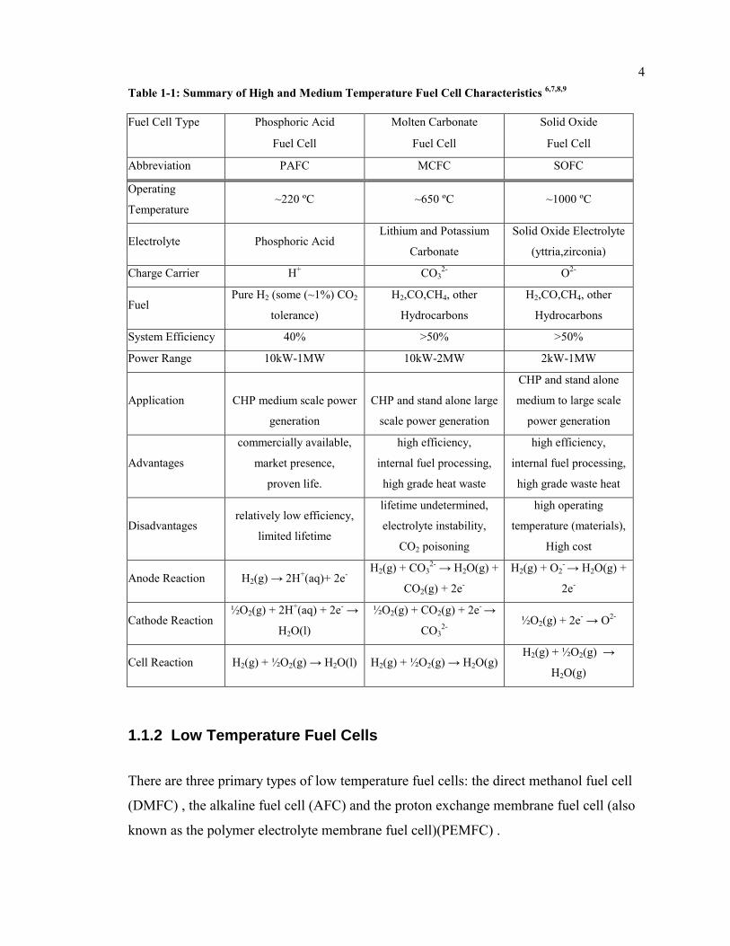
4Table 1-1: Summary of High and Medium Temperature Fuel Cell Characteristics 6,7,8,9

Fuel Cell Type Phosphoric Acid Molten Carbonate Solid Oxide

Fuel Cell Fuel Cell Fuel Cell

Abbreviation PAFC MCFC SOFC

Operating

Temperature ~220 ºC ~650 ºC ~1000 ºC

Electrolyte Phosphoric Acid Lithium and Potassium

Carbonate

Solid Oxide Electrolyte

(yttria,zirconia)

Charge Carrier H+ CO32- O2-

Fuel Pure H2 (some (~1%) CO2

tolerance)

H2,CO,CH4, other

Hydrocarbons

H2,CO,CH4, other

Hydrocarbons

System Efficiency 40% >50% >50%

Power Range 10kW-1MW 10kW-2MW 2kW-1MW

Application CHP medium scale power

generation

CHP and stand alone large

scale power generation

CHP and stand alone

medium to large scale

power generation

Advantages

commercially available,

market presence,

proven life.

high efficiency,

internal fuel processing,

high grade heat waste

high efficiency,

internal fuel processing,

high grade waste heat

Disadvantages relatively low efficiency,

limited lifetime

lifetime undetermined,

electrolyte instability,

CO2 poisoning

high operating

temperature (materials),

High cost

Anode Reaction H2(g) → 2H+(aq)+ 2e- H2(g) + CO3

2- → H2O(g) +

CO2(g) + 2e-

H2(g) + O2- → H2O(g) +

2e-

Cathode Reaction ½O2(g) + 2H+(aq) + 2e- →

H2O(l)

½O2(g) + CO2(g) + 2e- →

CO32-

½O2(g) + 2e- → O2-

Cell Reaction H2(g) + ½O2(g) → H2O(l) H2(g) + ½O2(g) → H2O(g) H2(g) + ½O2(g) →

H2O(g)

1.1.2 Low Temperature Fuel Cells

There are three primary types of low temperature fuel cells: the direct methanol fuel cell

(DMFC) , the alkaline fuel cell (AFC) and the proton exchange membrane fuel cell (also

known as the polymer electrolyte membrane fuel cell)(PEMFC) .

5

Table 1-2: Summary of Low Temperature Fuel Cell Characteristics 6,7,8,9

Fuel Cell Type Proton Exchange Direct Methanol Alkaline

Membrane Fuel Cell Fuel Cell Fuel Cell

Abbreviation PEMFC DMFC AFC

Operating

Temperature 60-120 ºC 70-90 ºC 50-200 ºC

Electrolyte Solid Polymer (i.e. Nafion) Solid Polymer KOH

Charge Carrier H+ H+ OH-

Fuel Pure H2 (some CO2

tolerance) Pure H2 (some CO2 tolerance) Pure H2

System Efficiency 35-45% 35-40% 35-55%

Power Range 5-250 kW <1 kW <5kW

Desired

Application

Transportation, portable,

and low power CHP

applications

Transportation and portable

applications

Space (NASA) and some

other transportation

Advantages

high power densities,

proven long operating life,

adoption by automakers

reduced system complexity

(fuel reforming, compression,

and humidification are

eliminated)

inexpensive materials,

CO tolerance,

fast cathode kinetics

Disadvantages

lack of CO tolerance,

water and heat management,

expensive catalyst

anode kinetics, cross-over,

complex stack structure,

noble catalyst required

corrosive liquid electrolyte,

lack of CO2 tolerance

Anode Reaction H2(g) → 2H+(aq) + 2e- CH3OH(aq) + H2O(l) →

CO2(g) + 6H+(aq) + 6e-

H2(g) + 2(OH)-(aq) →

2H2O(l) + 2e-

Cathode Reaction ½O2(g) + 2H+(aq) + 2e- →

H2O(l)

6H+(aq) + 6e- + 3/2 O2(g) →

3H2O(l)

½O2(g) + H2O(l) + 2e- →

2(OH)-(aq)

Cell Reaction H2(g) + ½O2(g) → H2O(l) H2(g) + ½O2(g) → H2O(l) H2(g) + ½O2(g) → H2O(g)

AFCs were used by NASA for space missions, before NASA switched to PEMFCs.

AFCs were too expensive to be commercially viable for a long time but are currently

being investigated by several companies.

6

DMFCs are essentially quite similar to PEMFCs, and are currently being investigated

mostly for small portable power applications (i.e. laptop, cell phone, PDA, etc. battery

replacement). They are still encountering problems with fuel crossover.

1.1.3 Proton Exchange Membrane Fuel Cell (PEMFCs) PEMFC are currently being widely studied for use in a variety of transportation and

stationary applications.

Each cell in a PEMFC consists of two flow-field or collector plates (Figure 1.1) with a

membrane electrode assembly (MEA) (Figure 1.1) sandwiched between them (Figure

1.2). The MEA consists of a solid polymer electrolyte with a catalyst layer and a gas

diffusion layer (GDL) on each side. Generally the electrolyte is a solid polymer such as

Nafion®, the catalyst is carbon-supported platinum and the GDL is a woven or felted

material made of graphite fibers.

Hydrogen and oxygen (in the form of air or pure O2) are fed to the fuel cell through gas

flow channels on the anode and cathode flow-field plates respectively. At the anode,

hydrogen diffuses through the GDL to the catalyst layer and undergoes the following

reaction:

H2(g) → 2H+(aq) + 2e- Eq 1-1

The product protons pass through the solid polymer electrolyte membrane and the

electrons are forced through an external circuit, producing electricity.

At the cathode, oxygen diffuses through the GDL to the catalyst layer where it undergoes

the following reaction:

½O2(g) + 2H+(aq) + 2e- → H2O(l) Eq 1-2

7

Here each oxygen atom pairs with two protons, which have passed through the electrolyte

membrane, and two electrons, which have been forced through the external circuit, to

form a water molecule.

Figure 1.1: Membrane Electrode Assembly (left) and Graphite Flow-field Collector Plate (right) with Light Coloured Gasket.

8

Catalyst L

ayer

Catalyst L

ayerElectrolyte M

embrane

Gas D

iffusion Layer

Gas D

iffusion Layer

Membrane Electrode Assembly (MEA)

Fuel Gas Flow Channel


Oxidant Gas Flow Channel


Flow-Field Plate Flow-Field Plate

Catalyst L

ayer

Catalyst L

ayerElectrolyte M

embrane

Gas D

iffusion Layer

Gas D

iffusion Layer






Catalyst L

ayer

Catalyst L

ayerElectrolyte M

embrane

Gas D

iffusion Layer

Gas D

iffusion Layer

Catalyst L

ayer

Catalyst L

ayerElectrolyte M

embrane

Gas D

iffusion Layer

Gas D

iffusion Layer






Flow-Field Plate Flow-Field Plate

Figure 1.2: Single Cell Fuel Cell Assembly Cross Section

1.2 Fuel Cell Diagnostics

As with any other device there is an interest in knowing when and why a fuel cell is not

operating properly. This is information that needs to be understood not only for testing

and prototype development but also for quality control and monitoring during production.

This type of information is also needed for control and monitoring of onboard systems to

prevent catastrophic failure, or to correct poor operating conditions before equipment is

damaged.

The purpose of this work is to develop algorithms to identify fuel cell fault behaviour,

specifically using electrochemical impedance spectroscopy data from fuel cells under

9

fault conditions. This has been done to assist with the development of both onboard and

off-board fuel cell diagnostic hardware.

For the purposes of this work, an off-board diagnostic device would be external to the

fuel cell system and would be used to monitor fuel cell operation in specific settings

where there is more time and operator involvement. This would be similar to vehicle

diagnostic computers used currently by auto mechanics. An onboard diagnostic device

would be small and simple in order to be integrated into the fuel cell control system, not

only to identify which fault has occurred but also to initiate measures to resolve problems

before failure.

1.3 Background on fuel cell faults Like any other device, there are many ways that a fuel cell can fail. Some possible

mechanical failures in fuel cells include cracked flow-field plates, ruptured membranes or

leaking gaskets. In addition to mechanical failure, fuel cells are also susceptible to several

failure modes that either prevent the electrochemical reactions from occurring or slow

them down. These “electrochemical” faults can include problems with water management

such as the flooding of the electrode or the drying of the membrane as well as poisoning

of the catalyst layer. These last three faults were the focus of this work and are described

further below. Membrane/catalyst ageing is also a possible electrochemical fault but it is

not examined in this work.

1.3.1 Fuel Cell Water Management Faults Water management and water transport in the membrane have been extensively studied in

an effort to improve fuel cell performance and prevent drying and flooding failure.

Further information about fuel cell failures and their identification can be found in

Larminie and Dicks7, Mérida1, and Hoogers6.

101.3.1.1 Flooding

As a product of the PEMFC reaction, water is produced at the fuel cell cathode. If the fuel

cell is working well, the water is either used to properly humidify the polymer electrolyte

membrane, or it is evaporated and carried away by the oxidant stream, leaving the fuel

cell as water vapor. If this is not happening water can build up in the pores of the gas

diffusion electrodes and in the flow channels, preventing the diffusion of gases to the

electrode. In extreme cases the water buildup can completely block the flow channel. It

has been shown10 that the buildup of water in the flow channel to the point of blockage is

responsible for the characteristic saw-tooth voltage profile that is associated with cathode

flooding behaviour1. This voltage profile is quite different from the voltage behaviour of

other faults examined; it could be used as another diagnostic method for flooding

identification.

1.3.1.2 Drying

Polymer electrolyte membranes such as Nafion® need to be well humidified in order to

function properly. If the reactant gas streams are not sufficiently humidified, or if the fuel

cell temperature is kept too high, water in the membrane evaporates into the gas stream

and is removed from the fuel cell.

If there is a net flux of water out of a particular region in the membrane, then the

membrane resistivity in that area increases. As the resistivity of the region increases, the

thermal stresses also increase. If the temperature in the drying regions increases to the

melting point of the membrane material (usually referred to as “brown out conditions”)

then the membrane can burn and rupture. In these conditions not only is the ionic

conductivity of the membrane compromised, the reactant streams may mix in possibly

explosive ratios.

Drying is typically characterized by a decrease in voltage over time (Figure 3.6 and

Figure 3.9) Further information about the pathological effects of membrane drying can be

found in the work of Walter Mérida1. EIS has been used previously as a method for

11

measuring membrane resistance, it is often assumed that the real part of an impedance

measurement at 1kHz is representative of the membrane resistance.11 Water vapor sensors

can be diagnostic of the conditions leading to membrane drying, but EIS directly

measures the state of the membrane.

1.3.2 Catalyst Poisoning Faults A number of materials can poison the platinum catalyst and affect fuel cell operation. CO,

HCHO, HCOOH, and other molecules can all effectively poison the catalyst layer by

occupying catalyst sites that could otherwise be used for the PEMFC reaction. This is of

concern because hydrogen produced through reforming (particularly in onboard systems)

often contains these agents. This work only examines the poisoning effects of the CO

molecule.

The rate of catalyst poisoning is dependant on the concentration of the poisoning agent in

the gas stream. Catalyst poisoning, like drying, is characterized by a decrease in voltage

with time (Figure 3.15). Almost full recovery from CO poisoning conditions can be

achieved by the addition of a small amount of oxygen (typically >1% air) to the fuel

stream. During air bleed the oxygen bonds with the CO to produce CO2, thus freeing the

occupied catalyst sites.

Another diagnostic method for CO is to create a condition where CO would be stripped

from the anode and see if recovery occurs. If so there was CO poisoning; if not another

fault. Two methods of doing this are bleeding air into the fuel gas stream12 and applying

positive potential excursions to the anode.

12

2 Electrochemical Impedance Spectroscopy (EIS)

EIS is a very useful fuel cell diagnostic tool because it is non-invasive and can indicate

information about the status of elements inside the fuel cell (e.g., the membrane). Fuel

cells are sensitive to anything inside the cell, so it is difficult to determine if data from

instrumentation inside the cell is due to cell behaviour or due to the perturbing presence

of the instrumentation. EIS avoids this problem because it requires no instrumentation

inside the cell and the amplitude of the AC perturbation is small. EIS, as a single

technique, is able to identify several different failure modes. This makes if appealing

because, even though the instrumentation required for EIS can be cumbersome and

expensive, only one on-board diagnostic system is required.

Electrochemical impedance spectroscopy (EIS) was traditionally applied to the

determination of the double layer capacitance and in AC polarography13,14. Currently EIS

is used primarily to characterize the electrical properties of materials and interfaces with

electrically conducting electrodes15. EIS studies the system response to the imposition of

a small amplitude AC signal. Impedance measurements are taken at various frequencies

of applied AC signal. EIS has been shown to be effective in identifying fuel cell fault

conditions1.

2.1 Impedance

Within this work i=√-1.

An AC voltage (Eq 2-1) of a known frequency ω and magnitude V is imposed over a DC

voltage VDC in a cell.

)sin()( tVVtV ACDC ω+=

Eq 2-1

13

The resulting AC current (Eq 2-2) is measured and compared to the incoming signal. θ is

the phase difference between the applied voltage (V(t)) and the measured current (I(t)).

)sin()( θω ++= tIItI ACDC

Eq 2-2

The impedance of the system (Eq 2-3) , Z(ω), is defined as the ratio of the applied

voltage, in the frequency domain,(v(ω)) to the measured current (i(ω))

)()()(

ωωω

ivZ ≡

Eq 2-3

Impedance is a complex number:

Z = Z’ + i·Z” Eq 2-4

The magnitude of impedance, |Z|, can be expressed as follows:

22 )"()'(|| ZZZ +=

Eq 2-5

The phase of the impedance φ is defined as:

−= −

'"tan 1

ZZϕ

Eq 2-6

Where the negative sign is conventionally added to give a positive phase when Z’ is

positive and Z” is negative.

To facilitate comparison, in this work impedance is shown scaled to a single cell in a fuel

cell with a surface area of 1.0 cm2. The impedance was first scaled to the cell area (Acell)

by multiplying the measured impedance (Zm) by the cell area to determined the scaled

impedance (Z):

cellm AZZ ⋅=

Eq 2-7

14

In the case of data acquired from the 4-cell stack assembly, the data is also scaled by the

number of cells:

cell

cellm

nAZ

Z⋅

=

Eq 2-8

where ncell is the number of cells in the stack.

Because all impedances are scaled to area the impedance units are consistently in Ω·cm2.

In a practical device, the ability to detect a fault occurring in a single cell of a large stack

is required. More stack data under actual operating conditions is required to effectively

determine if EIS has this ability, and to determine how accurately a fault can be detected

with a given number of cells. This question is considered in the for membrane resistance

in Section 6.

Impedance data is typically represented in two types of plots: the Nyquist/Argand Plot

and the Bode Plot.

The Nyquist Plot, is a graphical portrayal of complex numbers in the Argand plane;

where the X-axis represents the real part and the Y-axis represents the imaginary part of

the complex number. In the case of plotting impedance data, the positive Y-axis

conventionally represents the negative imaginary portion of the impedance and there is a

complex impedance point for every frequency at which the impedance was measured,

creating a plot with impedance features. The shape of these impedance features is what is

indicative of failure modes in fuel cell impedance and is further discussed in Section 3.

15

0.0 0.1 0.2 0.3 0.4 0.5 0.6 0.7 0.8 0.9 1.0 1.1 1.2 1.3 1.40.0

-0.1

-0.2

-0.3

-0.4

Im(Z

) / Ω

·cm

2

Re(Z) / Ω·cm2

Figure 2.1: Nyquist/Argand representation of a typical fuel cell impedance spectrum (See Section

3.3)

The Bode Plot consists of two graphs: one with the phase of the admittance (the negative

phase of the impedance) (φ) on the Y-axis and the logarithmic frequency (log10(ω)) on the

X-axis, the other with the log of the magnitude of the impedance (log10|Z(ω)|) on the Y-

axis and the logarithmic frequency (log10(ω)) on the X-axis.

The majority of the fitting for this work was done using the Nyquist/Argand

representation of measured impedance spectra. This is because there are characteristic

impedance shapes which are much more evident in this representation.

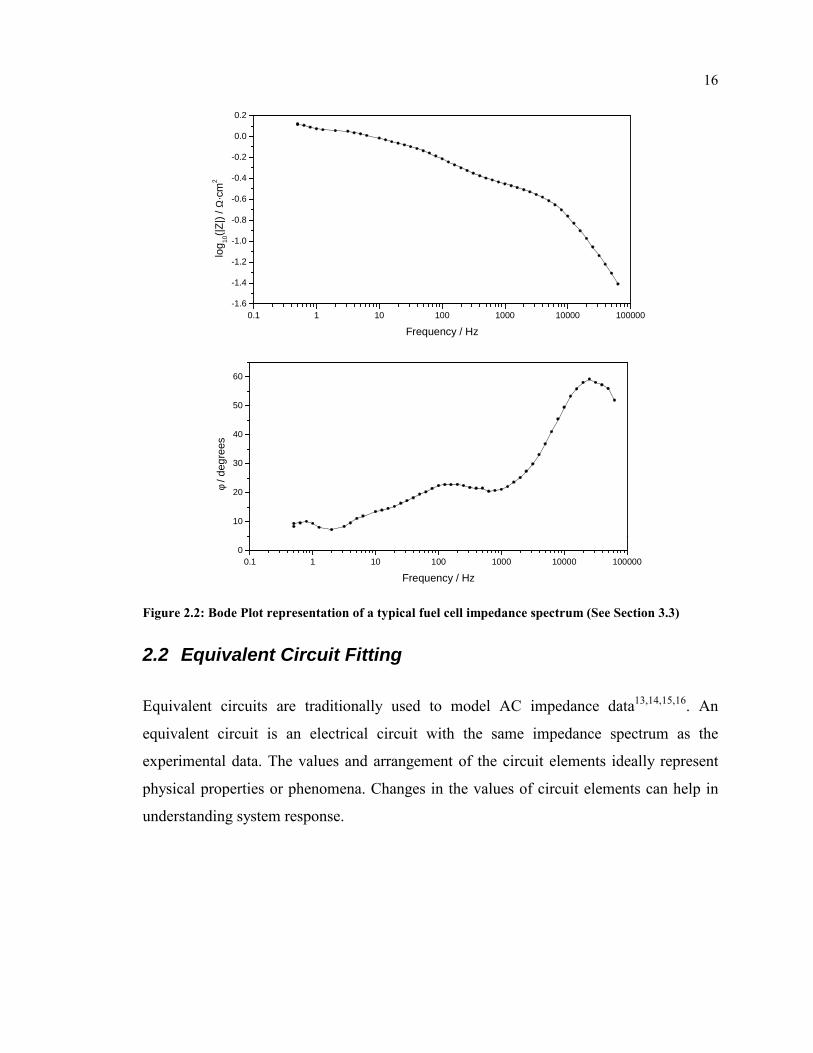
16

0.1 1 10 100 1000 10000 100000-1.6

-1.4

-1.2

-1.0

-0.8

-0.6

-0.4

-0.2

0.0

0.2

log 10

(|Z|)

/ Ω·c

m2

Frequency / Hz

0.1 1 10 100 1000 10000 1000000

10

20

30

40

50

60

φ / d

egre

es

Frequency / Hz

Figure 2.2: Bode Plot representation of a typical fuel cell impedance spectrum (See Section 3.3)

2.2 Equivalent Circuit Fitting

Equivalent circuits are traditionally used to model AC impedance data13,14,15,16. An

equivalent circuit is an electrical circuit with the same impedance spectrum as the

experimental data. The values and arrangement of the circuit elements ideally represent

physical properties or phenomena. Changes in the values of circuit elements can help in

understanding system response.

17

2.2.1 Background on equivalent circuit elements 2.2.1.1 Resistors

Eq 2-9 shows the expression for the impedance of a pure resistor, where R is the

resistance.

RZ R =

Eq 2-9

In the Nyquist plane a pure resistor appears as a single point on the real axis (Figure 2.3).

0.0 0.5 1.0 1.5 2.0

-1.0

-0.5

0.0

0.5

1.0ZR

Im(Z

) / Ω

·cm

2

Re(Z) / Ω·cm2

Figure 2.3: Nyquist Representation of the Impedance of a Pure Resistance (R=1Ω·cm2).

There are two primary types of resistances investigated for the equivalent circuit

modeling of fuel cells in this work: the electrolyte resistance and the charge transfer

resistance.

2.2.1.1.1 Electrolyte Resistance14,15

The electrolyte resistance (Rs), also referred to as the solution resistance, is the resistance

to current flow through the electrolyte. It is proportional to the electrolyte resistivity ρ,

and is dependant on the cell geometry (planar in this case) where d is the thickness of the

electrolyte (Eq 2-10).

18

dRS ⋅= ρ

Eq 2-10

The resistance to current flow, in the metal of the electrode, is referred to as the metal

resistance (RM). The ohmic resistance (RΩ ) is the sum of the electrolyte resistance and the

metal resistance (Eq 2-11).

ms RRR +=Ω

Eq 2-11

2.2.1.1.2 Charge-Transfer Resistance14,15,17

The charge transfer resistance (Rct) is the resistance associated with the charge transfer

mechanism for electrode reactions. This is the resistance to electrons crossing the

interface. It is defined as the partial derivative of the faradaic current density (jF) with

respect to potential (E) (Eq 2-12): 1−

∂∂=

EjR F

ct

Eq 2-12

2.2.1.2 Capacitors

Eq 2-13 shows the expression for the impedance of a pure capacitor, where C is the

capacitance:

ZC = (i·ω·C)-1 Eq 2-13

The impedance of a pure capacitor is entirely imaginary and negative (Figure 2.4).

19

-1.0 -0.5 0.0 0.5 1.00.0

-0.5

-1.0

-1.5

-2.0 ZC

Im(Z

) / Ω

·cm

2

Re(Z) / Ω·cm2

Figure 2.4: Nyquist Representation of the Impedance of a Pure Capacitance (C=1 F·cm-1).

There are two primary types of capacitances investigated for the equivalent circuit

modeling of fuel cells in this work: the double-layer capacitance and the geometric (bulk)

capacitance.

2.2.1.2.1 Double-Layer Capacitance14,15

The double layer capacitance (Cdl) arises from an electrical double-layer that forms at the

interface between the electrode and the electrolyte. Eq 2-14 shows the expression for the

double-layer capacitance where σE is the charge density at the electrode, E is the

interfacial potential, T is the temperature, p is the pressure, and µ is the chemical

potential:

µ

σ

,, pT

Edl E

C

∂∂

=

Eq 2-14

2.2.1.2.2 Geometric Capacitance14,15

The geometric (bulk) capacitance (CG) is the capacitance that arises between the two

electrodes in an electrochemical cell. In Eq 2-15, d is the characteristic distance between

20

the two electrodes, εr is the dielectric constant of the electrolyte, and εo is the permittivity

of vacuum:

dC ro

Gεε ⋅

=

Eq 2-15

2.2.1.3 Inductors

Eq 2-16 shows the expression for the impedance of a pure inductor, where L is the

inductance:

ZL = i·ω·L Eq 2-16

The impedance of a pure inductor is entirely imaginary and positive (Figure 2.5).

1.0

0.5

0.0

-0.5

-1.0

-1.0 -0.5 0.0 0.5 1.0

Im(Z

) / Ω

·cm

2

ZL

Re(Z) / Ω·cm2

Figure 2.5: Nyquist Representation of the Impedance of a Pure Inductor (L= 1 H.cm-1)

Inductive behaviour in EIS data is often attributed to be an artifact due to cabling or

electrical equipment18.

2.2.1.4 Distributed Elements

Combinations of purely resistive, capacitive, or inductive behaviours do not necessarily

describe the response of all systems: to account for this distributed elements are used to

21

model behaviour. There are two principal forms of distributed elements that are closely

related: the constant phase element (CPE) and the Warburg element.

2.2.1.4.1 Constant Phase Elements (CPEs)

The impedance of a constant phase element (CPE) is expressed as follows, where T and φ

are CPE parameters: 1))(( −⋅= φωiTZCPE

Eq 2-17

The CPE can be used to describe pure resistor (φ = 0, T = R -1), a pure capacitor (φ = 1, T

= C), or a pure inductor (φ = -1, T = L-1). It is also associated with the Warburg element if

φ = 0.5.

0.0 0.1 0.2 0.3 0.4 0.5 0.6 0.7 0.8 0.9 1.00.0

-0.1

-0.2

-0.3

-0.4

-0.5

φ=0.7φ=0.8

φ=0.9

φ=0.6 φ=0.5φ=0.4

φ=0.3

φ=0.2

Im(Z

) / Ω

·cm

2

Re(Z) / Ω·cm2

φ=0.1

Figure 2.6: Nyquist Representation of Impedance of CPE with Varying φ Parameter (T Parameter =

1 F·cm-1·s-φ) for f = 0.5Hz to 25 kHz.

In general the impedance of CPEs is used to describe the double layer charging

characteristics of rough irregular electrode surfaces. The true physical significance of the

CPE with φ ≠ -1, 0, 0.5, or 1 has yet to be resolved but there are numerous attempts at

explanations for the physical meaning of CPEs.13-15, 19-32,20,21,22,

23,24, 25,26,27,28,29,30,31,32

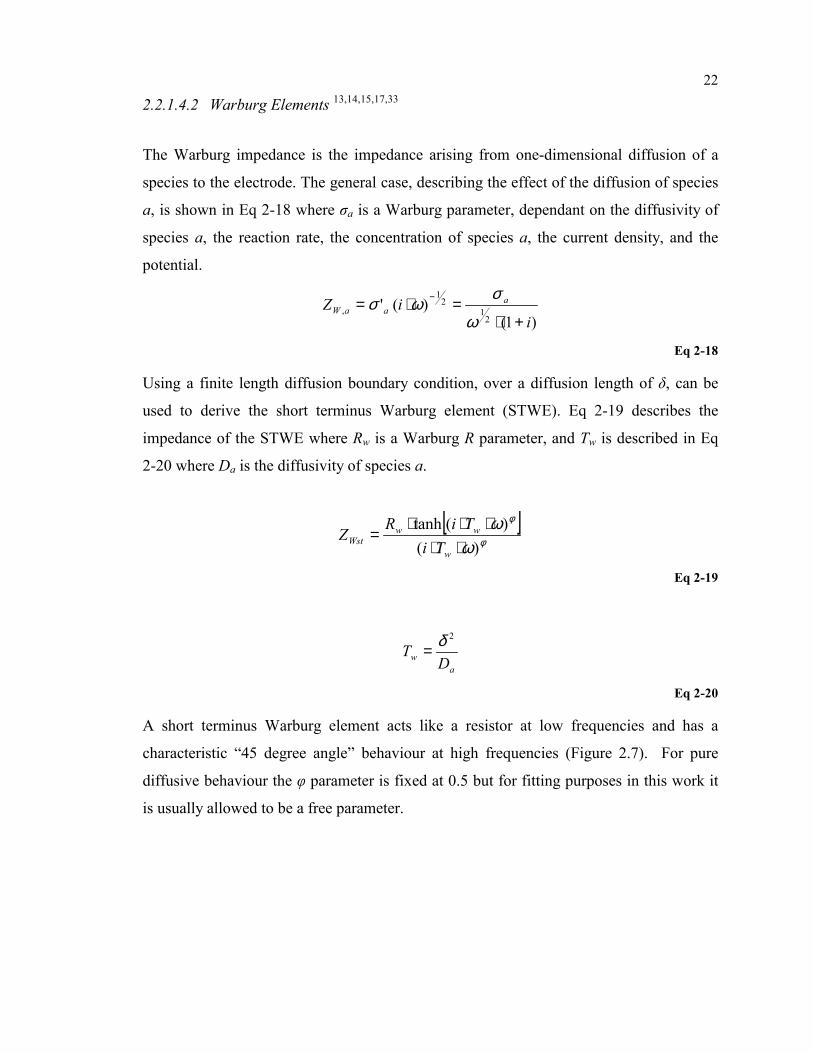
22

2.2.1.4.2 Warburg Elements 13,14,15,17,33

The Warburg impedance is the impedance arising from one-dimensional diffusion of a

species to the electrode. The general case, describing the effect of the diffusion of species

a, is shown in Eq 2-18 where σa is a Warburg parameter, dependant on the diffusivity of

species a, the reaction rate, the concentration of species a, the current density, and the

potential.

)1()('

21

21

,i

iZ aaaW

+⋅=⋅= −

ω

σωσ

Eq 2-18

Using a finite length diffusion boundary condition, over a diffusion length of δ, can be

used to derive the short terminus Warburg element (STWE). Eq 2-19 describes the

impedance of the STWE where Rw is a Warburg R parameter, and Tw is described in Eq

2-20 where Da is the diffusivity of species a.

[ ]φ

φ

ωω

)()(tanh

⋅⋅⋅⋅⋅

=w

wwWst Ti

TiRZ

Eq 2-19

aw D

T2δ=

Eq 2-20

A short terminus Warburg element acts like a resistor at low frequencies and has a

characteristic “45 degree angle” behaviour at high frequencies (Figure 2.7). For pure

diffusive behaviour the φ parameter is fixed at 0.5 but for fitting purposes in this work it

is usually allowed to be a free parameter.

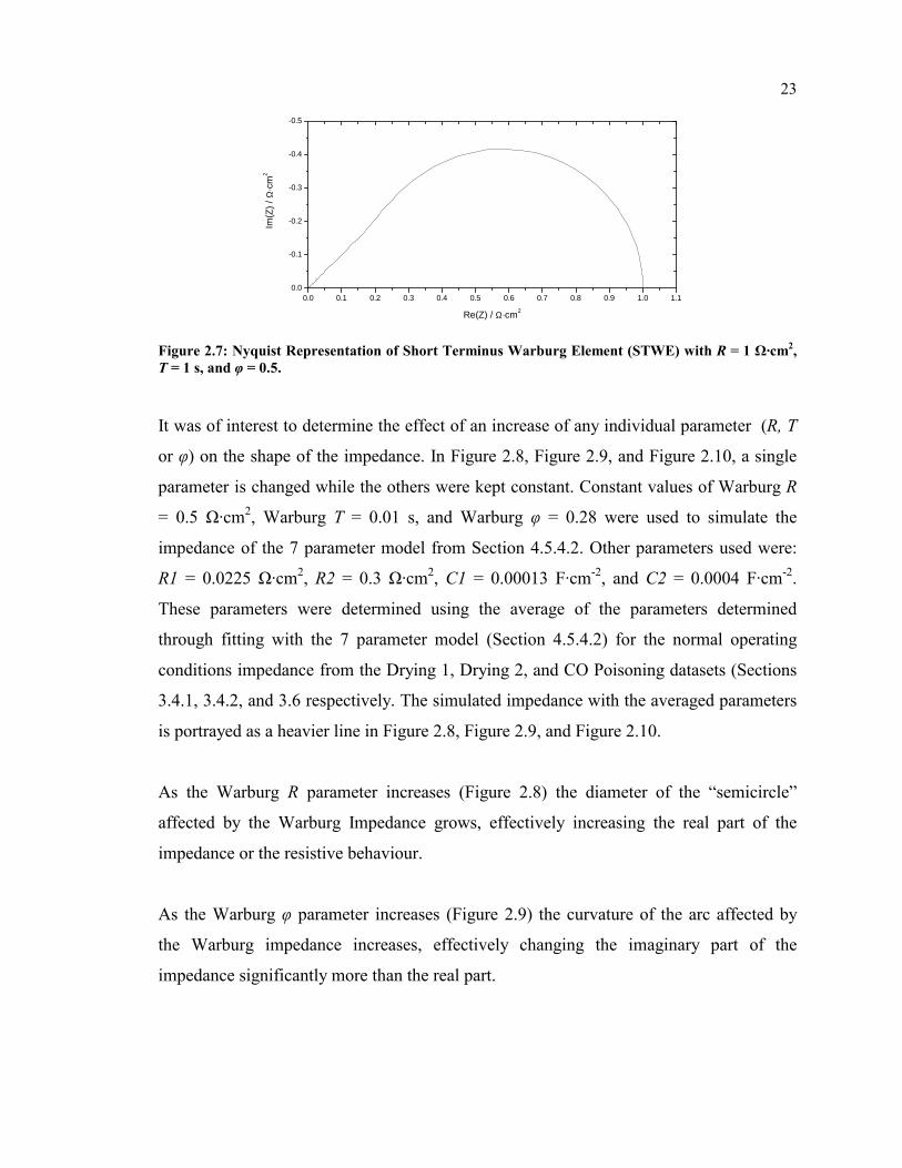
23

0.0 0.1 0.2 0.3 0.4 0.5 0.6 0.7 0.8 0.9 1.0 1.10.0

-0.1

-0.2

-0.3

-0.4

-0.5

Im(Z

) / Ω

·cm

2

Re(Z) / Ω·cm2

Figure 2.7: Nyquist Representation of Short Terminus Warburg Element (STWE) with R = 1 Ω·cm2, T = 1 s, and φ = 0.5.

It was of interest to determine the effect of an increase of any individual parameter (R, T

or φ) on the shape of the impedance. In Figure 2.8, Figure 2.9, and Figure 2.10, a single

parameter is changed while the others were kept constant. Constant values of Warburg R

= 0.5 Ω·cm2, Warburg T = 0.01 s, and Warburg φ = 0.28 were used to simulate the

impedance of the 7 parameter model from Section 4.5.4.2. Other parameters used were:

R1 = 0.0225 Ω·cm2, R2 = 0.3 Ω·cm2, C1 = 0.00013 F·cm-2, and C2 = 0.0004 F·cm-2.

These parameters were determined using the average of the parameters determined

through fitting with the 7 parameter model (Section 4.5.4.2) for the normal operating

conditions impedance from the Drying 1, Drying 2, and CO Poisoning datasets (Sections

3.4.1, 3.4.2, and 3.6 respectively. The simulated impedance with the averaged parameters

is portrayed as a heavier line in Figure 2.8, Figure 2.9, and Figure 2.10.

As the Warburg R parameter increases (Figure 2.8) the diameter of the “semicircle”

affected by the Warburg Impedance grows, effectively increasing the real part of the

impedance or the resistive behaviour.

As the Warburg φ parameter increases (Figure 2.9) the curvature of the arc affected by

the Warburg impedance increases, effectively changing the imaginary part of the

impedance significantly more than the real part.

24

As the Warburg T parameter increases (Figure 2.10) the diameter of the “semicircle”

affected by the Warburg impedance gets smaller, effectively decreasing the real part of

the impedance at lower frequencies.

All of these parameters also affect the overlap between the impedance features associated

with the Warburg element and other impedance features. This is of interest because this

overlap is affected greatly during CO poisoning but less so during drying.

0.51.0

1.5

0.0

-0.5

-1.0

-1.5

0.0

0.2

0.4

0.6

0.81.0

War

burg

R P

aram

eter

/ Ω

·cm

2

Im(Z

) / Ω

·cm

2

Re(Z) / Ω·cm2

Figure 2.8: Change in impedance shape of simulated Model 2 impedance with changing Warburg R parameter

25

0.0 0.5 1.0 1.5

0.0

-0.5

-1.0

-1.5

0.0

0.2

0.4

0.6

0.81.0

War

burg

φ Pa

ram

eter

Im(Z

) / Ω

·cm

2

Re(Z) / Ω·cm2

Figure 2.9: Change in impedance shape of simulated Model 2 impedance with changing Warburg φ parameter

0.2 0.4 0.6 0.8 1.00.0

-0.2

-0.4

-0.6

-0.8

-1.0

0.00

0.05

0.10

0.150.20

0.25

War

burg

T P

aram

eter

/ s

Im(Z

) / Ω

·cm

2

Re(Z) / Ω·cm2

Figure 2.10: Change in impedance shape of simulated Model 2 impedance with changing Warburg T parameter

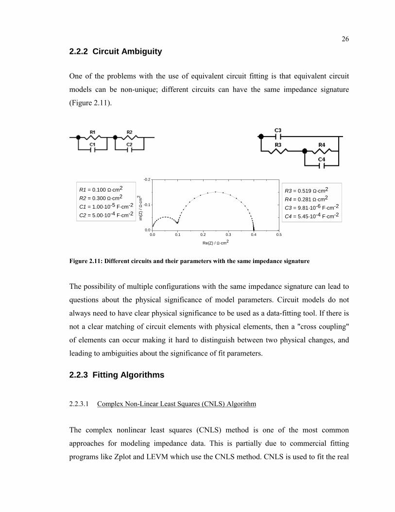
26

2.2.2 Circuit Ambiguity

One of the problems with the use of equivalent circuit fitting is that equivalent circuit

models can be non-unique; different circuits can have the same impedance signature

(Figure 2.11).

0.0 0.1 0.2 0.3 0.4 0.50.0

-0.1

-0.2

R1 = 0.100 Ω·cm2

R2 = 0.300 Ω·cm2

C1 = 1.00·10-5 F·cm-2

C2 = 5.00·10-4 F·cm-2

Im(Z

) / Ω

·cm

2

Re(Z) / Ω·cm2

R3 = 0.519 Ω·cm2

R4 = 0.281 Ω·cm2

C3 = 9.81·10-6 F·cm-2

C4 = 5.45·10-4 F·cm-2

Figure 2.11: Different circuits and their parameters with the same impedance signature

The possibility of multiple configurations with the same impedance signature can lead to

questions about the physical significance of model parameters. Circuit models do not

always need to have clear physical significance to be used as a data-fitting tool. If there is

not a clear matching of circuit elements with physical elements, then a "cross coupling"

of elements can occur making it hard to distinguish between two physical changes, and

leading to ambiguities about the significance of fit parameters.

2.2.3 Fitting Algorithms

2.2.3.1 Complex Non-Linear Least Squares (CNLS) Algorithm

The complex nonlinear least squares (CNLS) method is one of the most common

approaches for modeling impedance data. This is partially due to commercial fitting

programs like Zplot and LEVM which use the CNLS method. CNLS is used to fit the real

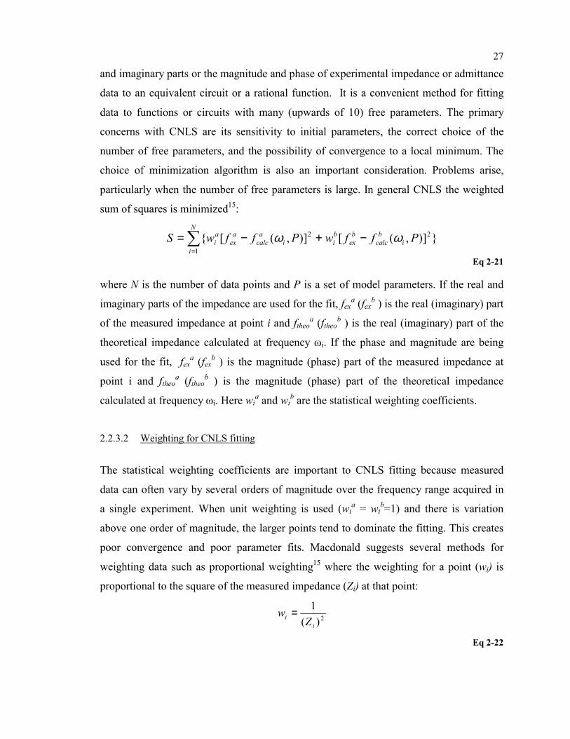
27

and imaginary parts or the magnitude and phase of experimental impedance or admittance

data to an equivalent circuit or a rational function. It is a convenient method for fitting

data to functions or circuits with many (upwards of 10) free parameters. The primary

concerns with CNLS are its sensitivity to initial parameters, the correct choice of the

number of free parameters, and the possibility of convergence to a local minimum. The

choice of minimization algorithm is also an important consideration. Problems arise,

particularly when the number of free parameters is large. In general CNLS the weighted

sum of squares is minimized15:

)],([)],([ 22

1PffwPffwS i

bcalc

bex

bii

acalc

aex

N

i

ai ωω −+−=∑

=

Eq 2-21

where N is the number of data points and P is a set of model parameters. If the real and

imaginary parts of the impedance are used for the fit, fexa (fex

b ) is the real (imaginary) part

of the measured impedance at point i and ftheoa (ftheo

b ) is the real (imaginary) part of the

theoretical impedance calculated at frequency ωi. If the phase and magnitude are being

used for the fit, fexa (fex

b ) is the magnitude (phase) part of the measured impedance at

point i and ftheoa (ftheo

b ) is the magnitude (phase) part of the theoretical impedance

calculated at frequency ωi. Here wia and wi

b are the statistical weighting coefficients.

2.2.3.2 Weighting for CNLS fitting

The statistical weighting coefficients are important to CNLS fitting because measured

data can often vary by several orders of magnitude over the frequency range acquired in

a single experiment. When unit weighting is used (wia = wi

b=1) and there is variation

above one order of magnitude, the larger points tend to dominate the fitting. This creates

poor convergence and poor parameter fits. Macdonald suggests several methods for

weighting data such as proportional weighting15 where the weighting for a point (wi) is

proportional to the square of the measured impedance (Zi) at that point:

2)(1

ii Z

w =

Eq 2-22

28

In function proportional weighting34, 35 the weighing is proportional to the function fitting

parameters and thus varies with each fitting iteration. Boukamp suggests using modulus

weighting36 (wi =1/(|Zl|+ |Zh|)1/2) where |Zl| and |Zh| are the vector lengths of the impedance

at the highest and lowest frequency. Another version of this method 36 uses |Zl| and |Zh| as

the absolute values of the real and imaginary impedance function at a point.

The choice of weighting function will depend heavily on the characteristics and error

distribution of the measured impedance data itself and the parameters being sought.

2.2.3.3 Initial Values for CNLS Fitting

Initial values are critical to the quality of fit of CNLS because of its iterative nature. If

they are not close to the real values, the CNLS fit may not reach convergence. The fit

may also converge on local, rather than global, minimum. One method for determining

starting values is through trial and error; using several different sets of starting values in

an attempt to reach convergence on a single circuit. If convergence is reached, to different

parameters, with differing starting values the better starting values can be chosen by

comparing the fit results with the χ2 statistical test (Section 2.2.4.1).

Another method is to build the model by fitting fewer elements and adding on more until

a model with good initial values is built. These methods will work on some equivalent

circuits with a small number of elements or relatively predictable initial values, but are

not efficient for more complex problems. Other methods used in the past are geometric

interpolation and grid methods37

2.2.3.4 Minimizing Algorithms for CNLS

There are several algorithms that can be used to minimize CNLS fitting functions. The

most commonly used algorithm in the software packages38 is the Levenberg-Marquardt

algorithm, but others like genetic algorithms and combinatorial optimization can also be

29

used depending on the number of allowable iterations and the quality of the initial

parameters

In the gradient method, minima are found by finding the steepest slope and searching in

that direction. This can be slow to converge. This method also has a relatively small

search area and can easily converge on local minima. The Levenberg-Marquardt

algorithm performs an interpolation between the Taylor series and the gradient methods

of minimizing least squares functions 39. In this algorithm the direction of search is

determined by solving for the search vector. This algorithm only looks in the direction of

the search vector. Because it only searched in one direction, convergence on a local

minima rather than the global one is possible. It has the advantage of relatively fast

convergence and relatively few iterations necessary, particularly if good initial values are

provided.

2.2.4 Statistical Comparison

The objective of the statistical analysis in this work is to determine if the addition of an

additional parameter to a model improves the fit of that model to a single spectrum in a

statistically significant manner. Adding a parameter to a model usually gives a better fit

(lower sum of squares) but this improvement may not always be statistically significant.

To determine when the addition of a parameter is statistically significant, a statistical test

on the F-ratio was applied.

2.2.4.1 Chi-Squared Test

The Chi-Squared Test is a measure of the goodness of fit of a model compared to

experimental data. χ2 is defined as follows:

[ ]∑=

−≡N

iii

i

xyy2

1

22

2 )(1σ

χ

Eq 2-23

30

where i indexes individual data points, σi2 is the variance of the parent distribution for

each data point, yi are the data, y(xi) are the fitted function values, and N is the number of

frequencies at which the impedance was measured in a spectrum. In this case, for i=1...N,

yi will be the real part of the impedance for each individual frequency in the spectrum.

For i=N+1…2N, yi will be the imaginary part of the impedance for each individual

frequency in the spectrum.

The error relating to the impedance at different frequencies is known to be uncorrelated.

This error can depend on the measurement system, for example errors might depend on

the magnitude of the signal measured due to range changing. One simple model could be

that the percent error is constant for all data points, leading to a larger absolute error for

larger impedances. Therefore the standard deviation for a replicate measurement can

depend on the frequency. In general, there is a different parent distribution (and variance

σi2) for each frequency. Furthermore the errors in the real and imaginary part of the data

points at each frequency are known to be uncorrelated for impedance data acquired with

an FRA setup40 but correlated for impedance acquired with a lock-in amplifier setup41.

All spectra used for statistical comparison were acquired with the FRA setup (Section

3.1.3.1).

In the fitting scheme the weighting for a given data point i should be chosen to be

inversely proportional to the known or estimated variance σi2. Since in our case, the

magnitude did not change significantly with frequency, unit weighting was chosen. This

implicitly assumes that σi is independent of i, allowing for the comparison of the fit of an

individual spectrum to several models with the F-test. Under these assumptions the χ2 and

sum of squares quantities are proportional.

2.2.4.2 F- Test for Additional Terms

Normally the F-test is used to test if two observed standard deviations come from the

same population. For data regression use, as here, it is used to determine if addition of a

parameter is significant. In our context, the F-Test is used only to compare the fit of a

31

single spectrum to different models, not to compare different spectra. An F-ratio can be

calculated to determine how much the addition of a parameter improves the fit 42. The

ratio is defined as followsi:

)2/()()()1(

2

22

nNnnnFx −

−−=χ

χχ

Eq 2-24

where Fx is the F-ratio, n is the number of parameters in the model, and 2N is the number

of points in the experimental dataset.

If the fit is substantially better then χ2 is smaller and the F-ratio is larger. The F-Test is a

statistical test on whether or not the F-ratio could be that large by chance. The null

hypothesis of this test is that an F-ratio this large could have arisen by chance.

The F-ratio is a statistic which follows the F distribution with ν1 = 1 and ν2 = 2N – n. The

F-ratio can be used with an F-distribution table to determine a F values by looking up

F(2N – n, 1). This value can then be used to look up the probability of achieving the same

fit or better by chance in F probability tables: PF(F, 1, 2N - n).

For example, if a function with k parameters and a function with k+1 parameters are

being compared, the function with k+1 parameters should be accepted if Fx(k+1) > Fx(k),

and rejected if Fx(k+1) << Fx(k). If Fx(k+1) ≈ Fx(k) then a judgment must be made as to

whether the new model or old model better describes the system. If this likelihood (PF) is

small (typically <1%) the addition of the new parameter was reasonable, otherwise it was

not statistically significant.

Maple’s F-function was used to compare equivalent circuit models using the F-Test,

because some F-tables do not cover the ranges of degrees of freedom required in our

work, and because it avoided manual interpolation between table values.

i Eq 2-24 is adapted from the equation found in reference 42 because it is used for polynomial fitting with a constant term in their context but not in ours.

32

3 Data The analysis rather than the experimental acquisition of fuel cell fault condition data was

the purpose of this work, but a description of the experimental data used is necessary to

understand its interpretation. All the data used in this work was acquired by Dr. Jean-

Marc Le Canut for the Greenlight Power Systems. A further discussion of the

experimental methods, conditions, and rationale for all the data used in this work can be

found in the work of Mérida1, and the Greenlight Power Systems reports by Le Canut et

al.2,3,4,5

3.1 Summary of Experimental Setup The experimental setup used to acquire the experimental impedance data used in this

work consists of 3 primary components: the fuel cell test station, the fuel cell stack, and

the EIS equipment. Below there is a brief overview of these components. A more in-

depth description of the experimental setup is beyond the scope of this work but can be

found in Refs.1 and 2.

3.1.1 Fuel Cell Test Station1,2

The fuel cell test station was manufactured by ASA Automation Systems (now

Greenlight Power Technologies) for Ballard Power Systems. The test station provides

conditioned fuel and oxidant streams to the fuel cell2,43 with the possibility of the delivery

of nitrogen to the cell. The pressure and flow of these gases are controlled through

pressure regulators, rotameters, and flow meters. The station also delivers deionized

water. The test station controls the cooling and heating of the cell through a control loop.

An attached humidification test station allows the control of the temperature and

humidification of the reactant gases, independent for fuel and oxidant streams. A

33

manifolding systems allows for the independent delivery of dry or humidified gases to the

fuel cell, or individual cells in the case of the fuel cell stack. The fuel cell test station

allows for the monitoring of the cell voltage and gas temperatures through a DAQ (Data

Acquisition System ) and a Labview program.

The test station is kept in a fume hood, and there are hydrogen sensors and safeguards as

well as a CO alarm in the room for safety reasons.

Figure 3.1: Fuel Cell Test Station.

3.1.2 Fuel Cell Stack

Two fuel cell stack test rigs were used to acquire the data used in this project. All the fault

datasets (Sections 3.4-3.7) were acquired using the single cell test rig. The varied gas

composition datasets (Section 3.8) were acquired using the four-cell stack test rig.

34

3.1.2.1 Single Cell Test Rig

The single cell test rig is made of a single cell: two graphite flow-field plates with an

MEA between them, sealed with gaskets. This cell is placed between two current

collectors, made of gold plated copper. The cell temperature is controlled through two

stainless steel parts, sandwiching the current collectors, that allow for cooling/heating

with deionized water. They also allow the passage of the fuel and oxidant gasses. This

assembly is held together by two large aluminum plates, separated from the cell by

insulating plates, connected to each other by threaded rods. Pressure can be applied to a

stack by a sliding piston in the upper aluminum plate which uses pressurized nitrogen.

Figure 3.2: Single Cell Stack Assembly

3.1.2.2 Four Cell Test Rig

The four cell test rig is quite similar to the single cell test rig. The major differences are

that there are four cells used instead of one, and that the fuel, oxidant, and cell

cooling/heating water are controlled independently for each cell. In depth discussion

regarding the design and function of the four cell stack can be found in Ref. 1.

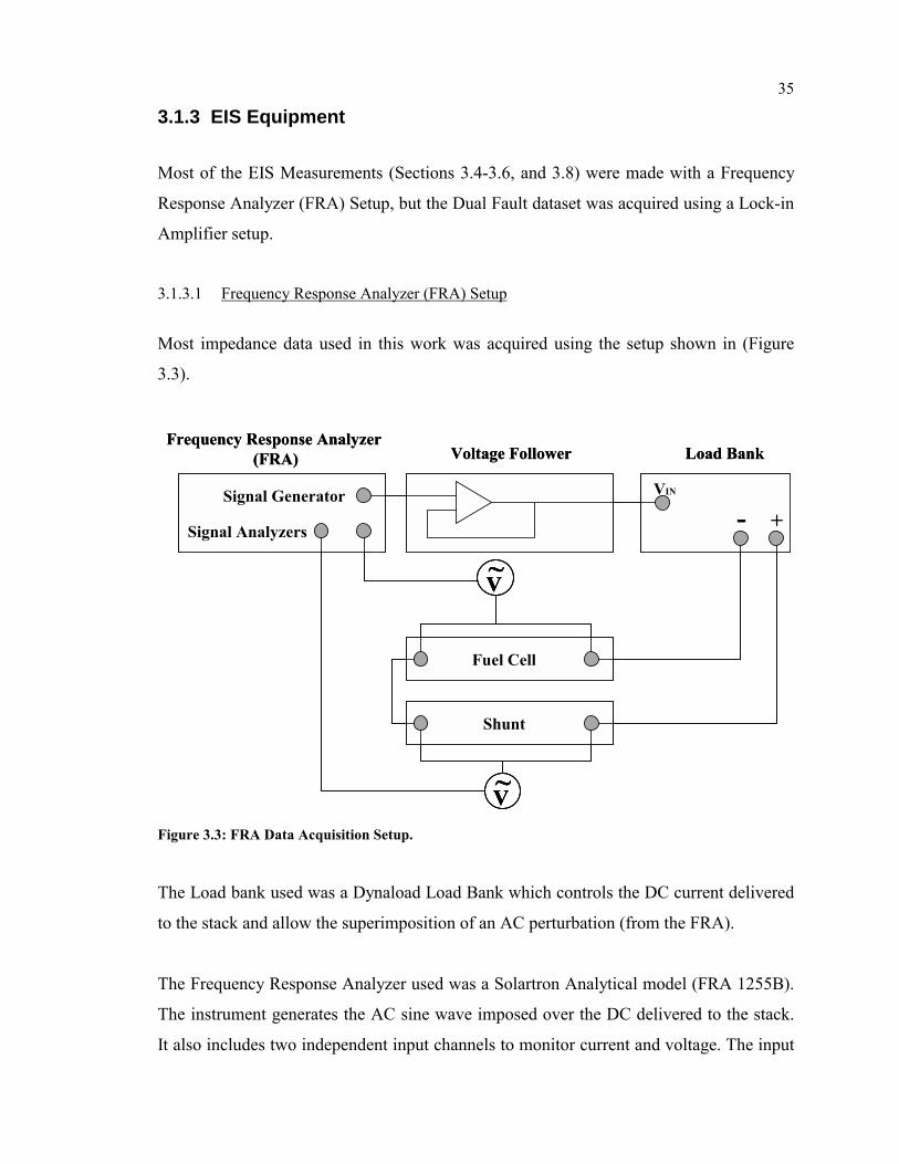
35

3.1.3 EIS Equipment

Most of the EIS Measurements (Sections 3.4-3.6, and 3.8) were made with a Frequency

Response Analyzer (FRA) Setup, but the Dual Fault dataset was acquired using a Lock-in

Amplifier setup.

3.1.3.1 Frequency Response Analyzer (FRA) Setup

Most impedance data used in this work was acquired using the setup shown in (Figure

3.3).

Frequency Response Analyzer (FRA) Voltage Follower Load Bank

VIN

+-Signal Generator

Signal Analyzers

Fuel Cell

V~

Shunt

V~

Frequency Response Analyzer (FRA) Voltage Follower Load Bank

VIN

+-Signal Generator

Signal Analyzers

Fuel Cell

V~V~V~

Shunt

V~V~V~

Figure 3.3: FRA Data Acquisition Setup.

The Load bank used was a Dynaload Load Bank which controls the DC current delivered

to the stack and allow the superimposition of an AC perturbation (from the FRA).

The Frequency Response Analyzer used was a Solartron Analytical model (FRA 1255B).

The instrument generates the AC sine wave imposed over the DC delivered to the stack.

It also includes two independent input channels to monitor current and voltage. The input

36

channel measuring voltage is connected across the fuel cell and the input channel

measuring current is connected across the shunt. Care was taken with the placement of

the cabling.

The FRA is controlled though a computer using an IEEE488 interface board and a

commercial software package: Zplot ™. Another software package, Zview ™, was used

to view and analyze impedance data.

3.1.3.2 Lock-in Amplifier (LIA) Setup 5

Two E.G.& G. Instruments 7265 DSP lock-in amplifiers (LIAs) were used for some

impedance acquisition. The setup used is shown in Figure 3.4.

DC Generator Electronic AdderLoad Bank

VIN + -

Fuel Cell

Shunt

DCIN

ACIN

VOUT VOUT

A

A

B/I

B/I

Ref

Ref

Osc.

Osc.

LIA - E

LIA - I


VIN + -

Fuel Cell

Shunt

DCIN

ACIN

VOUT VOUT

A

A

B/I

B/I

Ref

Ref

Osc.

Osc.

LIA - E

LIA - I


VIN + -

Fuel Cell

Shunt

DCIN

ACIN

VOUT VOUT

A

A

B/I

B/I

Ref

Ref

Osc.

Osc.

LIA - E

LIA - I

Figure 3.4: Lock-in Amplifier Impedance Acquisition Setup44.

3.2 Definitions for Dataset Terms The term spectrum will be used to describe a single set of impedance points measured at

individual frequencies, acquired consecutively, in a single experiment.

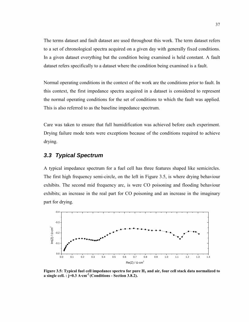
37

The terms dataset and fault dataset are used throughout this work. The term dataset refers

to a set of chronological spectra acquired on a given day with generally fixed conditions.

In a given dataset everything but the condition being examined is held constant. A fault

dataset refers specifically to a dataset where the condition being examined is a fault.

Normal operating conditions in the context of the work are the conditions prior to fault. In

this context, the first impedance spectra acquired in a dataset is considered to represent

the normal operating conditions for the set of conditions to which the fault was applied.

This is also referred to as the baseline impedance spectrum.

Care was taken to ensure that full humidification was achieved before each experiment.

Drying failure mode tests were exceptions because of the conditions required to achieve

drying.

3.3 Typical Spectrum A typical impedance spectrum for a fuel cell has three features shaped like semicircles.

The first high frequency semi-circle, on the left in Figure 3.5, is where drying behaviour

exhibits. The second mid frequency arc, is were CO poisoning and flooding behaviour

exhibits; an increase in the real part for CO poisoning and an increase in the imaginary

part for drying.

0.0 0.1 0.2 0.3 0.4 0.5 0.6 0.7 0.8 0.9 1.0 1.1 1.2 1.3 1.40.0

-0.1

-0.2

-0.3

-0.4

Im(Z

) / Ω

·cm

2

Re(Z) / Ω·cm2

Figure 3.5: Typical fuel cell impedance spectra for pure H2 and air, four cell stack data normalized to a single cell. : j=0.3 A·cm-2 (Conditions - Section 3.8.2).

38

3.4 Drying Datasets Two Drying datasets were chosen as being representative for this work. Both were

acquired with hydrogen as the fuel and air as the oxidant. Section 3.7 describes another

dataset which includes a drying sequence using reformate as the fuel and air as the

oxidant. Although both these drying datasets exhibit periodic drying and recovery

behaviour, their EIS signature is the same as for non oscillating drying behaviour1. This

oscillation is therefore not due to an artifact such as droplets blocking the inlet.

3.4.1 Drying 1 3 This drying dataset was acquired by maintaining the cell temperature higher than the gas

temperature (Table 3-1). This caused the partial pressure of the water vapour to decrease

and limited the humidification of the cell3. For this experiment impedance was recorded

continuously, taking about 3 minutes per spectra, with spectra recorded one after another.

The potential was recorded between acquisitions of spectra. Table 3-1 lists the

experimental conditions for the Drying 1 experiment.

Table 3-1: Drying 1 Experimental Conditions

Fuel Oxidant j MEA MEA anode Pt cathode Pt pfuel pox Tcell Tfuel Tox Min f Max f

A·cm2 Man. Material mgPt·cm-2 mgPt·cm-2 psig psig ˚C ˚C ˚C Hz kHz

H2 Air 0.4 MER Nafion 115 0.5 1 30 30 80 70 70 0.5 250

Figure 3.6 shows the fluctuation of cell voltage with drying. The cell voltage decreases

and partly recovers periodically. This is also reflected in the change in the size of the high

frequency impedance arc, which gets larger as the voltage decreases (Figure 3.8). There is

little change in the shape of the low frequency arcs with the exception of when the

voltage changes abruptly during acquisition of an impedance spectra (t =12 min).

39

0 5 10 15 20 25 30 35 400.30

0.35

0.40

0.45

0.50

0.55

0.60

0.65

0.70

0.75

0.80

E / V

t / min

Figure 3.6: Drying 1 – Change in Cell Voltage with Time.

0.00 0.25 0.50 0.75 1.000.00

-0.25

-0.50

0

5

10

15

20

25

30

35

40

t / m

in

Im(Z

) / Ω

·cm

2

Re(Z) / Ω·cm2 Figure 3.7: 3-D Nyquist for Drying 1 Dataset Impedance with Time.

0.0 0.1 0.2 0.3 0.4 0.5 0.6 0.7 0.8 0.9 1.00.0

-0.1

-0.2

-0.3

t = 2.5 min t = 5 min t = 8 min t = 12 min

Im(Z

) / Ω

·cm

2

Re(Z) / Ω·cm2

40

0.0 0.1 0.2 0.3 0.4 0.5 0.6 0.7 0.8 0.9 1.00.0

-0.1

-0.2

-0.3

t = 16 min t = 18 min t = 20 min t = 23 min t = 27 min

Im(Z

) / Ω

·cm

2Re(Z) / Ω·cm2

0.0 0.1 0.2 0.3 0.4 0.5 0.6 0.7 0.8 0.9 1.00.0

-0.1

-0.2

-0.3

t = 29 min t = 32 min t = 35 min t = 39 min

Im(Z

) / Ω

·cm

2

Re(Z) / Ω·cm2 Figure 3.8: Change in Drying 1 Dataset Impedance with Time.

3.4.2 Drying 2 3

This drying dataset was acquired by maintaining the cell temperature (Tcell = 90˚C ) higher

than the gas temperature (Table 3-2). For this experiment, impedance was recorded

continuously, taking about 2.5 minutes per spectra, with spectra recorded one after

another. The potential was recorded between the acquisition of spectra. The experimental

conditions for the Drying 2 dataset are shown in Table 3-2.

Table 3-2: Drying 2 Experimental Conditions


A·cm2 Man. Material mgPt·cm-2 mgPt·cm-2 psig psig ˚C ˚C ˚C Hz kHz

H2 Air 0.4 MER Nafion 115 0.5 1 30 30 90 70 70 50 250

The frequency range for acquisition was reduced in order to focus on the high frequency

impedance (where the effect of drying is most evident in the impedance). This also

reduces acquisition time since lower frequency measurements take more time.

Figure 3.9 shows the fluctuation of cell voltage with drying. As in the Drying 1 dataset

(Section 3.4.1), the cell voltage decreases and partly recovers periodically. This is also

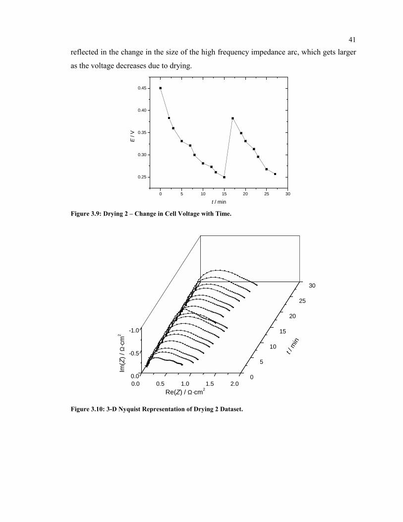
41

reflected in the change in the size of the high frequency impedance arc, which gets larger

as the voltage decreases due to drying.

0 5 10 15 20 25 30

0.25

0.30

0.35

0.40

0.45

E / V

t / min Figure 3.9: Drying 2 – Change in Cell Voltage with Time.

0.0 0.5 1.0 1.5 2.00.0

-0.5

-1.0

0

5

10

15

20

25

30

t / m

in

Im(Z

) / Ω

·cm

2

Re(Z) / Ω·cm2

Figure 3.10: 3-D Nyquist Representation of Drying 2 Dataset.

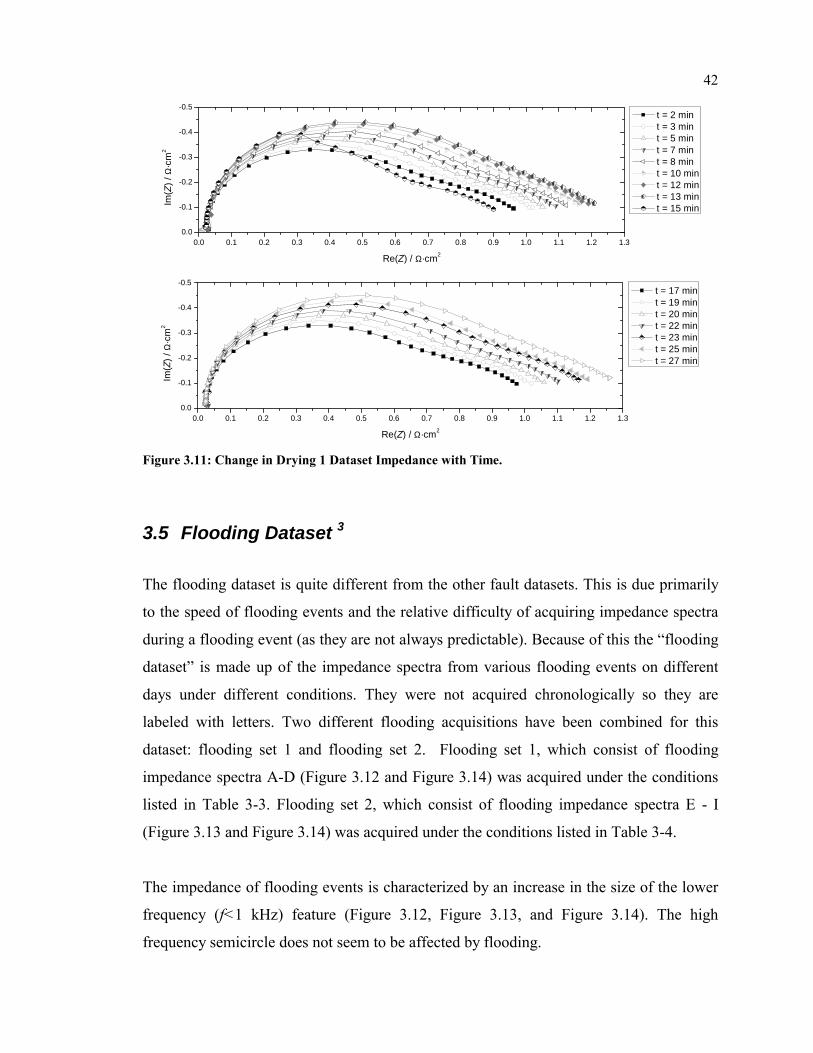
42

0.0 0.1 0.2 0.3 0.4 0.5 0.6 0.7 0.8 0.9 1.0 1.1 1.2 1.30.0

-0.1

-0.2

-0.3

-0.4

-0.5

Im(Z

) / Ω

·cm

2

Re(Z) / Ω·cm2

t = 2 min t = 3 min t = 5 min t = 7 min t = 8 min t = 10 min t = 12 min t = 13 min t = 15 min

0.0 0.1 0.2 0.3 0.4 0.5 0.6 0.7 0.8 0.9 1.0 1.1 1.2 1.30.0

-0.1

-0.2

-0.3

-0.4

-0.5

Im(Z

) / Ω

·cm

2

Re(Z) / Ω·cm2

t = 17 min t = 19 min t = 20 min t = 22 min t = 23 min t = 25 min t = 27 min

Figure 3.11: Change in Drying 1 Dataset Impedance with Time.

3.5 Flooding Dataset 3

The flooding dataset is quite different from the other fault datasets. This is due primarily

to the speed of flooding events and the relative difficulty of acquiring impedance spectra

during a flooding event (as they are not always predictable). Because of this the “flooding

dataset” is made up of the impedance spectra from various flooding events on different

days under different conditions. They were not acquired chronologically so they are

labeled with letters. Two different flooding acquisitions have been combined for this

dataset: flooding set 1 and flooding set 2. Flooding set 1, which consist of flooding

impedance spectra A-D (Figure 3.12 and Figure 3.14) was acquired under the conditions

listed in Table 3-3. Flooding set 2, which consist of flooding impedance spectra E - I

(Figure 3.13 and Figure 3.14) was acquired under the conditions listed in Table 3-4.

The impedance of flooding events is characterized by an increase in the size of the lower

frequency (f<1 kHz) feature (Figure 3.12, Figure 3.13, and Figure 3.14). The high

frequency semicircle does not seem to be affected by flooding.

43

Table 3-3: Experimental Conditions for Flooding Data Files A-D (Flooding Set 1).


A·cm-2 Man. Material mgPt·cm-2 mgPt·cm-2 psig psig ˚C ˚C ˚C Hz kHz

H2 Air 0.5 MER Nafion 115 0.5 1 30 30 35 90 95 1 150

Table 3-4: Experimental Conditions for Flooding Data Files D-I (Flooding Set 2).



H2 Air varied MER Nafion 115 0.5 1 30 30 50 95 95 0.5 1000

0.0 0.2 0.4 0.6 0.8 1.0 1.2 1.40.0

-0.2

-0.4

-0.6

-0.8

-1.0

-1.2

After Purge (A) Semi-Flooded (B) Flooded (C) Flooded (D)

Im(Z

) / Ω

·cm

2 )

Re(Z) / Ω·cm2 Figure 3.12: Change in Fuel Cell Impedance with Flooding Conditions (Flooding Set 1).

0.0 0.2 0.4 0.6 0.8 1.0 1.2 1.4 1.6 1.8 2.00.0

-0.2

-0.4

-0.6

-0.8

-1.0

Before Flood (E) Semi Flooded (F) Semi Flooded (G) Flooded (H) Semi Flooded (I)

Im(Z

) / Ω

·cm

2

Re(Z) / Ω·cm2

Figure 3.13: Change in Fuel Cell Impedance with Flooding Conditions (Flooding Set 2).

44

0.00 0.25 0.50 0.75 1.00 1.25 1.50 1.750.00

-0.25

-0.50

AB

CD

EF

GH

I

Floo

ding

File

Im(Z

) / Ω

·cm

2

Re(Z) / Ω·cm2

Figure 3.14: : 3-D Nyquist Representation of Flooding Impedance Data.

3.6 CO Poisoning Datasets3

The CO Poisoning dataset was acquired by replacing hydrogen with reformate with 10

ppm CO as the fuel gas. The composition of the reformate used is: 70% H2, 24% CO2

24%, and 6% N2. While the fuel reformate (10ppm CO) was used as the fuel, the voltage

decreased for approximately 80 minutes. The voltage decreased fairly slowly for the first

hour and then more swiftly for another 20 minutes. At t = 80 min, approximately 1% air

was bled into the fuel compartment and the cell voltage recovered rapidly over 5 minutes.

Table 3-5 shows the experimental conditions for the CO poisoning experiment.

Table 3-5: CO Poisoning Experimental Conditions



H2 Ref 0.4 MER Nafion 115 0.5 1 30 30 60 70 70 0.5 250

As CO poisoning progresses the second semicircle feature of the impedance gets larger

while the first stays relatively the same.

45

0 20 40 60 80 100 120

0.0

0.1

0.2

0.3

0.4

0.5

0.6

E / V

t / min Figure 3.15: CO Poisoning – Change in Cell Voltage with Time.

0.0 0.5 1.0 1.5 2.0 2.5 3.0 3.5 4.00.0

-0.5

-1.0

-1.5

-2.0

0

20

40

60

80

100

120

t / m

in

Im(Z

) / Ω

·cm

2

Re(Z) / Ω·cm2

Figure 3.16: 3-D Nyquist Representation of CO Poisoning Dataset.

0.00 0.25 0.50 0.75 1.00 1.25 1.50 1.75 2.00 2.25 2.50 2.75 3.00 3.25 3.500.00

-0.25

-0.50

-0.75

120 min 133 min 148 min 163 min 179 min 194 min 209 min

Im(Z

) / Ω

·cm

2

Re(Z) / Ω·cm2

Figure 3.17: Change in CO Poisoning Dataset Impedance with Time (Selected Files) Before Recovery.

46

0.0 0.2 0.4 0.6 0.8 1.0 1.2 1.4 1.6 1.8 2.0 2.2 2.4 2.6 2.8 3.00.0

-0.2

-0.4

-0.6

-0.8 214 min 217 min 220 min 222 min 225 min 227 min 230 min 232 min 235 min

Im(Z

) / Ω

·cm

2

Re(Z) / Ω·cm2 Figure 3.18: Change in CO Poisoning Dataset Impedance with Time During and After Recovery with Air Bleed.

3.7 Dual Fault Dataset5

For the dual fault dataset the fuel cell was poisoned with CO, recovered, then dried. The

CO poisoning part of the dual fault dataset was acquired using the reformate with 10 ppm

CO as the fuel. The composition of the reformate used is: 70% H2, 24% CO2 24%, and

6% N2. At t = 80 min, approximately 1% air was bled into the fuel compartment and the

cell voltage recovered rapidly over 10 minutes. The fuel cell membrane was then dried by

switching the humidified fuel stream to a dry stream and by turning off the humidification

to the air stream. Table 3-6 shows the experimental conditions for the dual fault dataset.

Figure 3.19 and Figure 3.20 show the change in potential and impedance respectively

with time for the dual fault dataset.

Table 3-6: Experimental Conditions for Dual Fault Dataset.



Ref Air 0.3 MER Nafion 115 0.7 0.4 30 30 60 85 80 10 5

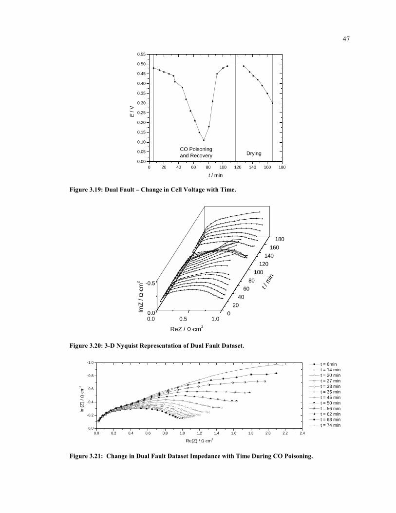
47

0 20 40 60 80 100 120 140 160 1800.00

0.05

0.10

0.15

0.20

0.25

0.30

0.35

0.40

0.45

0.50

0.55

DryingCO Poisoning and Recovery

E / V

t / min Figure 3.19: Dual Fault – Change in Cell Voltage with Time.

0.0 0.5 1.00.0

-0.5

020

4060

80100

120140

160180

t / m

in

ImZ

/ Ω·c

m2

ReZ / Ω·cm2

Figure 3.20: 3-D Nyquist Representation of Dual Fault Dataset.

0.0 0.2 0.4 0.6 0.8 1.0 1.2 1.4 1.6 1.8 2.0 2.2 2.40.0

-0.2

-0.4

-0.6

-0.8

-1.0

t = 6min t = 14 min t = 20 min t = 27 min t = 33 min t = 35 min t = 45 min t = 50 min t = 56 min t = 62 min t = 68 min t = 74 min

Im(Z

) / Ω

·cm

2

Re(Z) / Ω·cm2

Figure 3.21: Change in Dual Fault Dataset Impedance with Time During CO Poisoning.

48

0.0 0.2 0.4 0.6 0.8 1.0 1.2 1.4 1.6 1.8 2.00.0

-0.2

-0.4

-0.6

-0.8

-1.0

t = 81 min t = 86 min t = 92 min t = 100 min t = 106 min

Im(Z

) / Ω

·cm

2

Re(Z) / Ω·cm2 Figure 3.22: Change in Dual Fault Dataset Impedance with Time During CO Poisoning Recovery Due to Air Bleed.

0.0 0.2 0.4 0.6 0.8 1.0 1.2 1.4 1.6 1.80.0

-0.1

-0.2

-0.3

-0.4

-0.5

-0.6

t = 128 min t = 136 min t = 141 min t = 147 min t = 153 min t = 160 min t = 167 min

Im(Z

) / Ω

·cm

2

Re(Z) / Ω·cm2

Figure 3.23: Change in Dual Fault Dataset Impedance with Time During Drying Sequence.

3.8 Varying Gas Composition Datasets

The varying gas composition datasets were acquired using different gas compositions for

the fuel and oxidant streams and acquiring impedance spectra over a range of current

densities. Five combinations of gas compositions were used: H2-O2, H2-60% O2, H2-Air,

Reformate –60% O2, and Reformate-Air. All were acquired on the four cell stack

assembly, with the impedance of each cell measured. For data analysis purposes, only the

data from Cell 1 was used.

3.8.1 Pure Hydrogen and Oxygen (H2-O2)4

The conditions, polarization curves, and impedance diagrams for the H2-O2 experiment

are shown in Table 3-7, Figure 3.24, and Figure 3.25 respectively.

49Table 3-7: Experimental Conditions for H2-O2 Gas Composition Dataset.

Fuel Oxidant MEA MEA anode Pt cathode Pt pfuel pox Tcell Tfuel Tox Min f Max f

Man. Material mgPt·cm2 mgPt·cm2 psig psig ˚C ˚C ˚C Hz kHz

H2 O2 MER Nafion 115 0.7 0.4 30 30 65 85 70 0.5 50

0.0 0.1 0.2 0.30.4

0.5

0.6

0.7

0.8

0.9

1.0

Cell 1 Cell 2 Cell 3 Cell 4

j / A·cm-2

E / V

Figure 3.24: Polarization Curves for H2-O2 Gas Composition Dataset.

0.00 0.25 0.50 0.75 1.00 1.25 1.50 1.75 2.000.00

-0.25

-0.50

0.00

0.05

0.10

0.15

0.20

0.25

0.30

0.35

j / A·

cm-2

Im(Z

) / Ω

·cm

2

Re(Z) / Ω·cm2

Cell 1

0.00 0.25 0.50 0.75 1.00 1.25 1.50 1.75 2.000.00

-0.25

-0.50

0.00

0.05

0.10

0.15

0.20

0.25

0.30

0.3

j / A·

cm-2

ImZ

/ Ω·c

m2

Re(Z) / Ω·cm2

Cell 2

0.00 0.25 0.50 0.75 1.00 1.25 1.50 1.75 2.000.00

-0.25

-0.50

0.00

0.05

0.10

0.15

0.20

0.25

0.30

0.35

j / A·

cm-2

Im(Z

) / Ω

·cm

2

Re(Z) / Ω·cm2

Cell 3

0.00 0.25 0.50 0.75 1.00 1.25 1.50 1.75 2.000.00

-0.25

-0.50

0.00

0.05

0.10

0.15

0.20

0.25

0.30

0.35

j / A·

cm-2

Im(Z

) / Ω

·cm

2

Re(Z) / Ω·cm2

Cell 4

Figure 3.25: 3-D Nyquist Representations of H2-O2 Impedance Data.

50

3.8.2 Pure Hydrogen and Air (H2-Air)4 The conditions, polarization curves, and impedance diagrams for the H2-Air experiment

are shown in Table 3-8, Figure 3.26, and Figure 3.27 respectively.

Table 3-8: Experimental Conditions for H2-Air Gas Composition Dataset.


Man. Material mgPt·cm-2 mgPt·cm-2 psig psig ˚C ˚C ˚C Hz kHz

H2 Air MER Nafion 115 0.7 0.4 30 30 65 85 70 0.5 50

0.0 0.1 0.2 0.30.4

0.5

0.6

0.7

0.8

0.9

1.0


j / A.cm-2

E /

V

Figure 3.26: Polarization Curves for H2-Air Gas Composition Dataset.

51

0.00 0.25 0.50 0.75 1.00 1.25 1.50 1.75 2.00 2.250.00

-0.25

-0.50

0.00

0.05

0.10

0.15

0.20

0.25

0.30

0.35

j / Α·

cm-2

Im(Z

) / Ω

·cm

2

Re(Z) / Ω·cm2

Cell 1

0.00 0.25 0.50 0.75 1.00 1.25 1.50 1.75 2.00 2.250.00

-0.25

-0.50

0.00

0.05

0.10

0.15

0.20

0.25

0.30

0.35

j / Α

·cm-2

Im(Z

) / Ω

·cm

2

Re(Z) / Ω·cm2

Cell 2

0.00 0.25 0.50 0.75 1.00 1.25 1.50 1.75 2.00 2.250.00

-0.25

-0.50

0.00

0.05

0.10

0.15

0.20

0.25

0.30

0.35

j / Α·

cm-2

Im(Z

) / Ω

·cm

2

Re(Z) / Ω·cm2

Cell 3

0.00 0.25 0.50 0.75 1.00 1.25 1.50 1.75 2.00 2.250.00

-0.25

-0.50

0.00

0.05

0.10

0.15

0.20

0.25

0.30

0.35

j / A·

cm-2

Im(Z

) / Ω

·cm

2

Re(Z) / Ω·cm2

Cell 4

Figure 3.27: 3-D Nyquist Representations of H2-Air Impedance Data.

3.8.3 Pure Hydrogen and 60% Oxygen, 40 % Nitrogen (H2-O260%)4

The conditions, polarization curves, and impedance diagrams for the H2-60% O2

experiment are shown in Table 3-8, Figure 3.26, and Figure 3.27 respectively.

Table 3-9: Experimental Conditions for H2- 60% O2 Gas Composition Dataset.



H2

60% O2

40% N2 MER Nafion 115 0.7 0.4 30 30 65 85 70 0.5 50

52

0.00 0.05 0.10 0.15 0.20 0.25 0.30

0.4

0.5

0.6

0.7

0.8

0.9

1.0


j / A·cm-2

E / V

Figure 3.28: Polarization Curves for H2- 60% O2 Gas Composition Dataset.

0.00 0.25 0.50 0.75 1.00 1.25 1.50 1.75 2.000.00

-0.25

-0.50

0.00

0.05

0.10

0.15

0.20

0.25

0.30

0.35

j / Α·

cm-2

Im(Z

) / Ω

·cm

2

Re(Z) / Ω·cm2

Cell 1

0.00 0.25 0.50 0.75 1.00 1.25 1.50 1.75 2.000.00

-0.25

-0.50

0.00

0.05

0.10

0.15

0.20

0.25

0.30

0.35

j / Α·

cm-2

Im(Z

) / Ω

·cm

2

Re(Z) / Ω·cm2

Cell 2

0.0 0.5 1.0 1.5 2.00.00

-0.25

-0.50

0.00

0.05

0.10

0.15

0.20

0.25

0.30

0.35

j / Α

·cm-2

Im(Z

) / Ω

·cm

2

Re(Z) / Ω·cm2

Cell 3

0.00 0.25 0.50 0.75 1.00 1.25 1.50 1.75 2.000.00

-0.25

-0.50

0.00

0.05

0.10

0.15

0.20

0.25

0.30

0.35

j / Α·

cm-2

Im(Z

) / Ω

·cm

2

Re(Z) / Ω·cm2

Cell 4

Figure 3.29: 3-D Nyquist Representations of H2-60% O2 Impedance Data.

53

3.8.4 Reformate and 60% Oxygen, 40 % Nitrogen (Ref-O260%)4

The reformate used for this experiment was a mixture of the following composition: 70%

H2, 24% CO2 24%, and 6% N2. The conditions, polarization curves, and impedance

diagrams for the Ref –60% O2 experiment are shown in Table 3-10, Figure 3.30, and

Figure 3.31 respectively.

Table 3-10: Experimental Conditions for Ref - 60% O2 Gas Composition Dataset.



Ref

60% O2

40% N2 MER Nafion 115 0.7 0.4 30 30 65 85 70 0.5 50

0.00 0.05 0.10 0.15 0.20 0.25 0.30

0.4

0.5

0.6

0.7

0.8

0.9

1.0


j / A·cm-2

E / V

Figure 3.30: Polarization Curves for Ref- 60% O2 Gas Composition Dataset.

54

0.00 0.25 0.50 0.75 1.00 1.25 1.50 1.75 2.000.00

-0.25

-0.50

0.00

0.05

0.10

0.15

0.20

0.25

0.30

0.35

j (A·

cm2 )

ImZ

(Ω·c

m2 )

ReZ (Ω·cm2)

Cell 1

0.00 0.25 0.50 0.75 1.00 1.25 1.50 1.75 2.000.00

-0.25

-0.50

0.00

0.05

0.10

0.15

0.20

0.25

0.30

0.35

j / A·

cm-2

Im(Z

) / Ω

·cm

2

Re(Z) / Ω·cm2

Cell 2

0.00 0.25 0.50 0.75 1.00 1.25 1.50 1.75 2.000.00

-0.25

-0.50

0.00

0.05

0.10

0.15

0.20

0.25

0.30

0.35

j / A·

cm-2

Im(Z

) / Ω

·cm

2

Re(Z) / Ω·cm2

Cell 3

0.00 0.25 0.50 0.75 1.00 1.25 1.50 1.75 2.000.00

-0.25

-0.50

0.00

0.05

0.10

0.15

0.20

0.25

0.30

0.35

j / A·

cm-2

Im(Z

) / Ω

·cm

2

Re(Z) / Ω·cm2

Cell 4

Figure 3.31: 3-D Nyquist Representations of Ref-60% O2 Impedance Data.

3.8.5 Reformate and Air (Ref-Air)4

The reformate used for this experiment was a mixture of the following composition: 70%

H2, 24% CO2 24%, and 6% N2. The conditions, polarization curves, and impedance

diagrams for the Ref-Air experiment are shown in Table 3-11, Figure 3.32, and Figure

3.33 respectively.

Table 3-11: Experimental Conditions for Ref –Air Gas Composition Dataset.



Ref Air MER Nafion 115 0.7 0.4 30 30 65 85 70 0.5 50

55

0.00 0.05 0.10 0.15 0.20 0.25 0.30

0.4

0.5

0.6

0.7

0.8

0.9

1.0

1.1


j / A·cm-2

E / V

Figure 3.32: Polarization Curves for Ref- Air Gas Composition Dataset.

0.00 0.25 0.50 0.75 1.00 1.25 1.50 1.75 2.00 2.25 2.50 2.75 3.000.00

-0.25

-0.50

0.00

0.05

0.10

0.15

0.20

0.25

0.30

0.35

j / A·

cm-2

Im(Z

) / Ω

·cm

2

Re(Z) / Ω·cm2

Cell 1

0.00 0.25 0.50 0.75 1.00 1.25 1.50 1.75 2.00 2.25 2.50 2.75 3.000.00

-0.25

-0.50

0.00

0.05

0.10

0.15

0.20

0.25

0.30

0.35

j / A·

cm-2

Im(Z

) / Ω

·cm

2

Re(Z) / Ω·cm2

Cell 2

0.00 0.25 0.50 0.75 1.00 1.25 1.50 1.75 2.00 2.25 2.50 2.75 3.000.00

-0.25

-0.50

0.00

0.05

0.10

0.15

0.20

0.25

0.30

0.35

j / A·

cm-2

Im(Z

) / Ω

·cm

2

Re(Z) / Ω·cm2

Cell 3

0.00 0.25 0.50 0.75 1.00 1.25 1.50 1.75 2.00 2.25 2.50 2.75 3.000.00

-0.25

-0.50

0.00

0.05

0.10

0.15

0.20

0.25

0.30

0.35

j / A·

cm-2

Im(Z

) / Ω

·cm

2

Re(Z) / Ω·cm2

Cell 4

Figure 3.33: 3-D Nyquist Representations of Ref-Air Impedance Data.

56

4 Equivalent Circuit Model Development Equivalent circuit fitting has the ability to be quite useful as a fuel cell diagnostic

algorithm, particularly in an off-board setting. Through the possible relationship between

equivalent circuit element values and physical characteristics of the fuel cell, there is the

potential to identify not just fault conditions but also the part of the fuel cell affected.

Equivalent circuit fitting would be less useful in an onboard diagnostic device because of

the sensitivity to initial conditions (sufficiently so that one set of initial conditions would

not necessarily be useable for all operating conditions) and the time required to achieve

convergence.

As an initial basis for this work, fuel cell models from the literature were surveyed. These

models were examined, modified, and compared in an attempt to develop a model with

good fitting properties and logical physical significance. Models from the literature and

in-house models were used as the basis for modification through subtraction methods and

trial and error. All models were compared using the χ2 test for models with an equal

number of parameters and the F-test for models with different numbers of parameters.

4.1 Early In-House Models

Initial studies were performed using the model developed by Dr. Jean-Marc Le Canut in

earlier work on this project.44 This circuit (Figure 4.1) was used to model the PEMFC

impedance assuming that the impedance at the anode is small compared to the cathode

and membrane impedances. In Figure 4.1 the membrane resistance contributes to both

RΩ, and Rm, Cm is a capacitance associated with the membrane (likely the geometric

capacitance), and Wc is a Warburg parameter related to diffusion at the cathode:

57

RΩ

Cm

Rm Wc Figure 4.1: Early In-House Circuit 144.

This circuit was later used again as part of another model (Figure 4.2) where the anode

contribution is considered but diffusion is considered to be very fast at the anode while

the resistance is ignored at the cathode. In this model Cdl is the double layer capacitance.

RΩ

Rm Wc

Cm Cdl

Figure 4.2: Early In-House Circuit 244.

4.2 Models from the Literature Many equivalent circuit models can be found in the literature to describe the impedance

of fuel cells. Elements of these models were used in an attempt to fit our results but none

were more successful than later in-house models. Though PEM fuel cell impedance

models were the primary focus for the modeling in this work, models for solid oxide and

direct methanol fuel cell impedance were also investigated.

4.2.1 PEM Fuel Cells The PEM fuel cell models in the literature fall into two primary categories: entire fuel

cell models and membrane specific models.

584.2.1.1 Entire Fuel Cell Models Several groups have developed models for the impedance of operating PEM fuel cells.

4.2.1.1.1 Schiller et al.45,46 and Wagner et al.47,48 Models

Schiller et al. 45,46 and Wagner et al. 47 propose the model in Figure 4.3 to describe the

impedance of fuel cells during normal operating conditions 46 and during CO poisoning 45,47. In this model Lw is an inductance attributed to wiring, RΩ is the membrane

resistance, CPEdl-c, and CPEdl-a are approximations of the double-layer capacity at the

cathode and the anode respectively, Rct-c, and Rct-a are charge transfer resistances

associated with the cathode and the anode reactions respectively, and Zc is the finite

diffusion impedance. The Nernst impedance (ZN) is used to define the finite diffusion

impedance 47 (Eq 4-1). Here RW is the Warburg R parameter, Dk is the diffusion constant

(for diffusion of species k to the anode), and dN is the diffusion layer thickness:

( ) 2tanh −⋅⋅⋅

⋅=

Nk

wN dD

iiRZ ω

ω

Eq 4-1

Lw RΩRct-c Rct-a

CPEdl-a CPEdl-c

Zc

Figure 4.3: Model Proposed by Schiller et al. 45,46 and Later by Wagner et al. 47 to Describe the Impedance of Fuel Cells During CO Poisoning, and During “normal” Operation.

Another model was later proposed by Wagner et al. 48 (Figure 4.4) which is similar to the

model in Figure 4.3. All the elements have the same interpretation, with the exception of

the removal of the wiring inductance element (Lw) and the addition, on the anode circuit

branch, of a parallel “relaxation impedance” characterized by a series relaxation

resistance (RK) and pseudo-inductance (LK) which is defined in Eq 4-2 where τK is the

relaxation time constant.

59

KKK RL ⋅=τ

Eq 4-2

RΩ Rct-c

Rct-a

CPEdl-a

CPEdl-c

Zc

LKRK

Figure 4.4: Model Proposed by Wagner et al. 48 to Describe Fuel Cell Impedance During CO Poisoning.

4.2.1.1.2 Andreaus et al. Models49,50

Andreaus et al. have proposed both an idealized model for the only the fuel cell cathode50

(Figure 4.5) as well as for the entire fuel cell49 (Figure 4.6).

In Figure 4.5 RΩ is the membrane resistance, Cdl-c is the double layer capacitance

associated with the cathode, Rct-c is the charge transfer resistance associated with the

cathode reaction, and Wc is the Warburg impedance associated with the diffusion of

oxidant to the cathode.

RΩ

Cdl-c

Rct - c Wc Figure 4.5: Model Proposed by Andreaus et al. 50 to Describe the Cathode Impedance of Fuel Cells.

In Figure 4.6 RΩ is the membrane resistance, Cdl is the double layer capacitance of the

entire cell, Rct is the charge transfer resistance associated with the entire reaction, and ZN

is the Nernst impedance.

60

RΩ

Cdl

Rct, total

ZN

Figure 4.6: Model Proposed by Andreaus et al.5049 to Ideally Describe the Impedance of Fuel Cells.

4.2.1.1.3 Ciureanu et al. Models51,52,53

Ciureanu et al. 51,52,53 propose several models to describe the behaviour of fuel cells, with

a particular interest in the behaviour of the anode. They initially proposed a circuit

(Figure 4.7) to describe the anode and membrane impedance using an H2/H2 fed cell. In

the first paper51 the physical meaning of the parameters is addressed: RΩ is the membrane

resistance, C1 is the double layer capacitance, and R1 is the charge transfer resistance, and

C2 and R2 are described as the “capacitance and resistance of an adsorbed species”. The

other papers52,53 do not discuss the physical significance of parameters.

RΩ

R1R2

C1

C2

RΩ

R1R2

C1

C2

RΩ

R1R2

C1

C2

Figure 4.7: Model Proposed by Ciureanu et al. 51,52,53 for the Impedance of an H2/H2 fed Fuel Cell.

They also proposed a circuit (Figure 4.8) to describe the anode and membrane impedance

using an H2/H2+CO fed cell to model the effect of CO poisoning. For this circuit RΩ, R1,

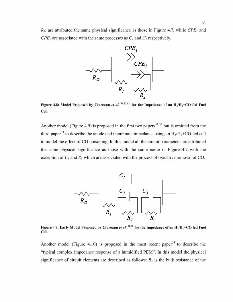
61

R1, are attributed the same physical significance as those in Figure 4.7, while CPE1 and

CPE2 are associated with the same processes as C1 and C2 respectively.

RΩ

R1R2

CPE2

CPE1

RΩ

R1R2

CPE2

CPE1

RΩ

R1R2

CPE2

CPE1

R1R2

CPE2

CPE1

Figure 4.8: Model Proposed by Ciureanu et al. 51,52,53 for the Impedance of an H2/H2+CO fed Fuel

Cell.

Another model (Figure 4.9) is proposed in the first two papers51,52 but is omitted from the

third paper53 to describe the anode and membrane impedance using an H2/H2+CO fed cell

to model the effect of CO poisoning. In this model all the circuit parameters are attributed

the same physical significance as those with the same name in Figure 4.7 with the

exception of C3 and R3 which are associated with the process of oxidative removal of CO.

RΩ

R1R2

C1

C2

R3

C3

RΩ

R1R2

C1

C2

R3

C3

Figure 4.9: Early Model Proposed by Ciureanu et al. 51,52 for the Impedance of an H2/H2+CO fed Fuel Cell.

Another model (Figure 4.10) is proposed in the most recent paper53 to describe the

“typical complex impedance response of a humidified PEM”. In this model the physical

significance of circuit elements are described as follows: R1 is the bulk resistance of the

62

specimen, C1 is the cell capacitance, and W is related to the diffusion of protons within

the membrane.

C1

R1 W

C1

R1 W Figure 4.10: Model Proposed by Ciureanu et al. 53 for the Impedance of an H2/O2 fed Fuel Cell.

4.2.1.2 Membrane Specific Models

There have been many groups who have studied and modeled the impedance of just the

MEA or the electrolyte. These studies differ from our work in that the MEA or electrolyte

is studied outside of a working fuel cell application.

4.2.1.2.1 Beattie et al. Model54

Beattie et al. 54 have studied the impedance of humidified BAM membranes in direct

contact with a gold electrode. They proposed the model in Figure 4.11 to describe the

impedance response for interface between the gold electrode and the electrolyte. In Figure

4.11 Rm and Cm are the membrane resistance and capacitance, respectively, Rc is the

contact resistance, Cdl is the double-layer capacitance, Rct is the charge transfer resistance,

and W is the Warburg impedance.

Rc

Rm W

Cm Cdl

Rct

Figure 4.11: Model Proposed By Beattie et al.54 for gold electrode/BAM membrane interface impedance.

63

4.2.1.2.2 Eikerling et al. Model 55

Eikerling et al. 55 model the catalyst layer as a one dimensional transmission line

equivalent circuit with Rp is the proton resistance, Rct is the charge transfer resistivity, Rel

is the electron resistance, and Cdl is the double layer capacitance.

Rp

Rct

Rel

Rp

Rct Rct Rct

Rp Rp

Rel Rel Rel

Cdl Cdl Cdl Cdl

H+

e-

Figure 4.12: Model Proposed by Eikerling et al. 55 to Model the Catalyst Layer.

4.2.1.2.3 Baschuk et al. Model 56

Baschuk et al propose a model for the ohmic losses at the fuel cell electrode and plate

interface (Figure 4.13).

Plate

R

Flow Channel

wc

ws

δc hc hp

Rs

Rs

Rs

Rf

Electrode

R

R

R

Figure 4.13: Model proposed by Baschuk et al. 56 to describe the effective equivalent electrical resistance of the electrode and flow-field plate.

64

In the Baschuk et al. model 56 the total resistance of the electrode (Rt - effectively ΣR

from Figure 4.13) can be expressed as follows:

)(8

,sc

cg

effeR

t wwln

R +⋅⋅⋅⋅

=δ

ρ

Eq 4-3

Where wc is the width of the flow channel, ws is the width of the flow plate support, ng is

the number of flow channels, δc is the thickness of the electrode, l is the length of the

electrode and ρR,eeff is described in Eq 4-4.

23

,,

)( e

eReffeR

l Φ−=

ρρ

Eq 4-4

Where ρR,e is the bulk resistivity of the electrode, and Φe is the void fraction of the

electrode.

The total resistance of the plate Rp is described by Baschuk et al. 56 as follows:

⋅−+⋅=

cg

cppRp wnW

hWh

LR ,ρ

Eq 4-5

Where ρR,p is the resistivity of the plate, hp is the height of the solid portion of the plates,

hc is the height of the flow channels, and W is the width of the plate.

4.2.2 Solid Oxide Fuel Cell (SOFC) Models

Equivalent circuits used to model SOFC impedance were also examined (Figure 4.14 to

Figure 4.17) because of similarities between published SOFC impedance data and

PEMFC experimental data. SOFC equivalent circuits were used to model data and

modified to develop further models. All the models below were used to fit our

experimental data from PEMFCs but none fit well enough to pursue further. Less focus

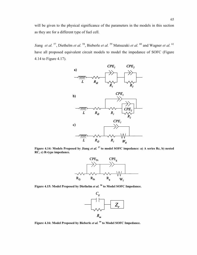
65

will be given to the physical significance of the parameters in the models in this section

as they are for a different type of fuel cell.

Jiang et al. 57, Diethelm et al. 58, Bieberle et al. 59 Matsuzaki et al. 60 and Wagner et al. 61

have all proposed equivalent circuit models to model the impedance of SOFC (Figure

4.14 to Figure 4.17).

L RΩR1 R2

CPE2CPE1a)

b)

L RΩ R1R2

CPE2

CPE1

RΩ R1 WR

CPE1

L

c)

L RΩR1 R2

CPE2CPE1a)

L RΩR1 R2

CPE2CPE1

L RΩR1 R2

CPE2CPE1a)

b)

L RΩ R1R2

CPE2

CPE1

RΩ R1 WR

CPE1

L

c)

b)

L RΩ R1R2

CPE2

CPE1

RΩ R1 WR

CPE1

L

c)

Figure 4.14: Models Proposed by Jiang et al. 57 to model SOFC impedance: a) A series Rc, b) nested RC, c) R-type impedance.

RΩ RPt Rg Wf

CPEgCPEPt

RΩ RPt Rg Wf

CPEgCPEPt

Figure 4.15: Model Proposed by Diethelm et al. 58 to Model SOFC Impedance.

Zr

Rm

Cg

Zr

Rm

Zr

Rm

Cg

Figure 4.16: Model Proposed by Bieberle et al. 59 to Model SOFC Impedance.

66

L

Cdl

ZdRb

Rc

W

L

Cdl

ZdRb

Rc

W

Cdl

ZdRb

Rc

W

ZdRb

Rc

W Figure 4.17: Model Proposed by Matsuzaki et al. 60 to Model SOFC Impedance.

RelRct-cRN-aRct-a

Cdl-cCN-aCdl-a

RelRct-cRN-aRct-a

Cdl-cCN-aCdl-a

Figure 4.18: Model Proposed by Wagner et al. 61 to Model SOFC Impedance.

4.2.3 Direct Methanol Fuel Cell Model

Müller et al. 62,63 have also done impedance studies on direct methanol fuel cells (DMFC)

that display some similarities to the work done on PEMFCs. Their equivalent circuit

model (Figure 4.19) has been used as a part of several of the modified models explored.

L

R∞

Cd

R0 L

R∞

Cd

R0

Figure 4.19: Model Proposed by Müller et al. 63 to Model DMFC Fuel Cell Anode Impedance Behavior.

This model was also used, on its own and as a series sub-circuit in data modeling but is

not a useful model alone for PEMFC experimental data.

67

4.3 Subtraction

A subtraction method was used as an approach to develop an equivalent circuit model

piece by piece from the experimental data. A model was developed using this method but

was later found to be flawed because of problems found with the precision of parameters

used in its development. The work using the subtraction method and subsequent problems

led to further work on the determination of the circuit parameters used to describe the

high frequency semi-circle (Section 6) but did not lead directly to a viable circuit.

When circuit elements are in series (Figure 4.20), the total impedance (Zt) is the sum of

the impedances of each of the series elements (Zi), where n is the number of series

elements:

∑=

=n

iit ZZ

1

Eq 4-6

Z1 Z2 Z3 Zn…Z1 Z2 Z3 Zn…

Figure 4.20: Circuit elements in series

This implies that a series element or branch can be removed by subtracting its impedance

from the total impedance to leave a remainder (ZR). So to determine the impedance

without the first series loop (Z1), Z1 is subtracted off the total impedance (Zt) to give the

remaining impedance (ZR):

1ZZZ tR −=

Eq 4-7

4.4 Trial and Error

A certain amount of educated trial and error was used to develop new models.

Components of models developed through subtraction and circuit equivalence as well as

from models found in the literature and early in-house models were combined to develop

new models.

68

4.5 Comparison Results

4.5.1 Model Comparisons for Non-Fault Condition Data

Early work was done fitting non-fault condition data. From this work models were

compared to determine the best model for non-fault condition impedance data. The

models chosen were determined to be the best fit through an averaging of the χ2

parameter for the fits to several spectra. The χ2 values shown are from a single

representative spectrum.

Through trial and error, modification, and comparison with the χ2 and F-Test statistics,

four models were found to be the best fits with 7, 8, and 9 parameters (Figure 4.21-Figure

4.23). These models were used to only fit data in the 50 Hz-50 kHz frequency range;

none of them fit the third semicircle feature. The physical features of the impedance data

led to these choices for the number of parameters. The shape of impedance data can also

be used as a simple indicator of the number and type of parameters for the equivalent

circuit to model it. For example, three semicircles indicate that a six-parameter model

(with three time constants) would be appropriate. In our case, two of the semicircles have

flattened sections, indicating the possibility of another parameter for the corresponding

semicircle, leading to an 8 or 9 parameter model for the entire impedance spectrum.

Sometimes the second semicircle has two poorly-resolved arcs which is why 7-9

parameter models were used to fit only in the 50 Hz to 50 kHz region. Models with more

than 9 parameters were examined but were found with the F-Test to not be statistically

significant improvements.

Figure 4.21: Best 7 parameter model from model modification tests: Model Mod 25; Chi-squared = 8.8051E-6, Sum of Weighted Squares = .00064277

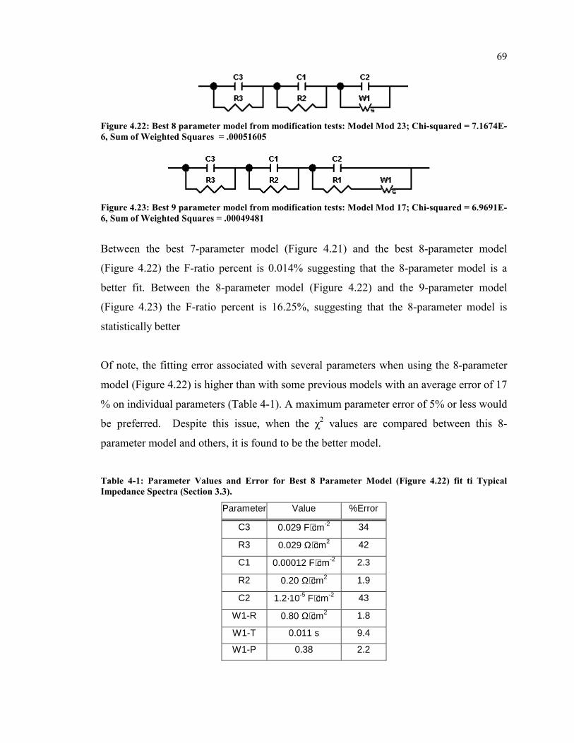
69

Figure 4.22: Best 8 parameter model from modification tests: Model Mod 23; Chi-squared = 7.1674E-6, Sum of Weighted Squares = .00051605

Figure 4.23: Best 9 parameter model from modification tests: Model Mod 17; Chi-squared = 6.9691E-6, Sum of Weighted Squares = .00049481

Between the best 7-parameter model (Figure 4.21) and the best 8-parameter model

(Figure 4.22) the F-ratio percent is 0.014% suggesting that the 8-parameter model is a

better fit. Between the 8-parameter model (Figure 4.22) and the 9-parameter model

(Figure 4.23) the F-ratio percent is 16.25%, suggesting that the 8-parameter model is

statistically better

Of note, the fitting error associated with several parameters when using the 8-parameter

model (Figure 4.22) is higher than with some previous models with an average error of 17

% on individual parameters (Table 4-1). A maximum parameter error of 5% or less would

be preferred. Despite this issue, when the χ2 values are compared between this 8-

parameter model and others, it is found to be the better model.

Table 4-1: Parameter Values and Error for Best 8 Parameter Model (Figure 4.22) fit ti Typical Impedance Spectra (Section 3.3).

Parameter Value %Error

C3 0.029 F⋅cm-2 34

R3 0.029 Ω⋅cm2 42

C1 0.00012 F⋅cm-2 2.3

R2 0.20 Ω⋅cm2 1.9

C2 1.2·10-5 F⋅cm-2 43

W1-R 0.80 Ω⋅cm2 1.8

W1-T 0.011 s 9.4

W1-P 0.38 2.2

70

Another 10-parameter model (Figure 4.24) has been explored as well for fitting the entire

spectrum. It was not compared statistically with other models because the range of

frequencies it fits is quite different.

Figure 4.24: 9 Parameter Model Which Fits the Entire Frequency Range.

0.0 0.1 0.2 0.3 0.4 0.5 0.6 0.7 0.8 0.9 1.00.0

-0.1

-0.2

-0.3

Im(Z

) (Ω

.cm

2 )

Re(Z) (Ω.cm2)

data fit

Figure 4.25: Nyquist Plot of Experimental Impedance Dataii and Fit with Full Frequency 9 Parameter Model (Figure 4.24)

4.5.2 Models for Fault Condition Impedance

The best models from the analysis on non-fault condition impedance data were used to

analyze the fault condition dataset impedance. Because CNLS is very sensitive to the

starting parameters for a fit, the same starting parameters were chosen for all the files in

each fault dataset. Starting parameters are the initial values of parameters which the

CNLS fitting algorithm uses as an initial “guess” to begin looking for convergence. The

initial set of starting parameters for a dataset was determined through fitting a standard

set of starting parameters to the initial “normal conditions” file in the dataset. In this

manner a consistent set of starting parameters was used for each file within a single fault

dataset, but different starting parameters were used for each fault dataset.

ii Spectrum conditions April 17 2002: H2/O2, T cell 70 ºC, Ballard MEA, j=0.4 A.cm-2.

71

4.5.3 Model for Entire Frequency Range

The full frequency 9 parameter model shown in Figure 4.24 was determined in to be a

good fit over the entire frequency range for normal operating conditions datasets. It was

also shown to be a good fit for drying fault datasets (χ2 = 8.5 × 10-5) but does not

converge for severe CO poisoning fault conditions.

At high levels of CO poisoning the Warburg and CPE parameters will not consistently

converge to specific values. This means that fits performed with converged fit parameter

values as starting values will not converge to similar values, if they converge at all. This

leads to concerns about this model’s suitability to fit CO poisoning impedance and thus as

a tool to differentiate between drying and CO poisoning faults.

4.5.4 Limited Frequency Range Models 4.5.4.1 8 Parameter Model

The 8 parameter model shown in Figure 4.22, which was shown to have statistically the

best fit of models attempted for non-fault condition datasets, will fit drying datasets ( χ2 =

2.8 × 10-5) but with some problems with the consistent convergence of the C2 parameter.

This model experiences similar problems to the 9 parameter model (Section 4.5.3) with

respect to fitting CO poisoning impedance data. Both the Warburg and C2 parameters

will not consistently converge. The problems with convergence for this model for both

drying and CO poisoning data prevent it from being an effective tool to differentiate

between drying and CO poisoning condition.

4.5.4.2 7 Parameter Model

The best, limited frequency, 7 parameter model (Figure 4.21) was investigated because of

the problems encountered fitting fault condition impedance data with the full frequency 9

parameter model, and the limited frequency 8 parameter model. The 7 parameter model

72

fits well for drying dataset (χ2 = 3.8 × 10-5) and well for CO poisoning datasets (χ2 = 5.3 ×

10-6). This model consistently converged for all CO poisoning and drying impedance

spectra.

4.5.4.3 Other Models

In the literature51,52,53 there is some suggestion that replacing capacitors in models which

fit normal PEM impedance with CPEs provides a better fit to CO poisoning impedance

data. Several models were developed (Figure 4.26-Figure 4.28) using this concept based

on the 7 parameter model (Figure 4.21). None of the models were a statistically

significant improvement over the 7 parameter model when the χ2 results for CO and

drying dataset fittings were compared straight on and using the F-test . Further

information about the F-Test can be found in Section 2.2.4.2.

The first model modification, and 8 parameter model, is not an improvement over the 7

parameter model (χ2 = 5.07E-06) as the χ2 value is higher. The second model

modification, also an 8 parameter model, is an improvement (has a lower χ2) but the

improvement is not sufficiently significant for a 56 degree of freedom system with an F-

ratio of 5.42 and an F-percent of 2.01%. The third model is a significant improvement

over the first and the second but its relationship to the 7 parameter model is difficult to

establish.

Figure 4.26: Equivalent Circuit Model Modification 1: Capacitor C1 from Figure 4.21 Replaced with a CPE. χ2 = 4.99E-05.

73Figure 4.27: Equivalent Circuit Model Modification2: Capacitor C2 from Figure 4.21 Replaced with a CPE χ2 = 4.60E-06.

Figure 4.28: Equivalent Circuit Model Modification 3: Capacitors C1 and C2 from Figure 4.21 Replaced with CPEs. χ2 = 3.53E-06.\

4.6 Conclusions Because of its relatively good ability to fit non-fault impedance data, and its ability to

converge on fault condition impedance data, the 7 parameter model shown in Figure 4.21

was chosen as the best model, of those attempted, for the purposes of differentiating

between drying and CO poisoning fault conditions.

74

5 Equivalent Circuit Model Results

The philosophy of our approach to equivalent modeling was to take a more empirical and

less physical approach. Parameters were only added if their statistical significance could

be proven. No attempts were made to determine anodic and cathodic contributions to the

fuel cell impedance through the equivalent circuit modeling, but this is certainly an area

for future work. More data from separate experiments measuring anode and cathode

impedances individually in a functioning fuel cell would really be required to

satisfactorily separate the contributions. This is outside of the diagnostic scope of this

work.

The equivalent circuit used in this work to generally model the impedance of fuel cells is

shown in Figure 4.21. Figure 5.1 shows the three sections of the circuit as they are

discussed in this section: Resistor R1, Parallel Resistor R2 and Capacitor C1, and Parallel

Capacitor C2 and Warburg W1.

Figure 5.1: Three Section of Equivalent Circuit Shown in Figure 4.21

All of the fault datasets described in Section 3 were fit with this circuit using ZView™,

an EIS data fitting program. This program uses a CNLS fitting algorithm to fit a specified

range of experimental impedance data to an equivalent circuit model. Unit weighting was

used as the weighting option. Each dataset was fit within the 50 Hz to 50 kHz frequency

range. The Drying1, Drying2, CO Poisoning, and Dual Fault dataset fit results for each

parameter are shown together on plots with time. Because the Flooding Dataset is not

chronological the fit results are shown on separate graphs.

75

For reference, Figure 5.2 shows the change in potential with time for the Drying1,

Drying2, CO Poisoning, and Dual Fault datasets. The degree of fault can, to some degree,

be indicated by the degree of decrease in potential.

0 20 40 60 80 100 120 140 160 1800.0

0.1

0.2

0.3

0.4

0.5

0.6

CO Poisoning Dataset Drying 1 Dataset Drying 2 Dataset Dual Fault Dataset

E / V

t / min

Figure 5.2: Potential Vs. Time for CO Poisoning, Drying 1, Drying 2, and Dual Fault Datasets.

5.1 Resistor R1

The resistance of the resistor R1 element is thought to be associated with a contact

resistance originating from contact between the GDL, electrode, and the collector plates.

This resistance can be seen on Nyquist representations as the real intercept of the high

frequency impedance with the Nyquist Re(Z) axis. Although the resistor R1 values

shows some small change with fault data and could possibly be used for diagnostics

based on that fact, it is likely that this change is due to a fitting artifact associated with the

fact that the frequency range of data fitted does not extend all the way to the real axis so

this is an extrapolated value. This is particularly apparent with the dual fault dataset R1

values where there is more variation and much smaller values. In this dataset the

impedance was only acquired up to 5 kHz so the spectra from the dual fault dataset could

not be fitted in the 5 kHz to 50 kHz regions, creating greater fitting error in the R1

parameter.

76

-- A B C D E F G H I-0.025

-0.020

-0.015

-0.010

-0.005

0.000

0.005

0.010

0.015

0.020

0.025

0.030

0.035

R1

/ Ω·c

m2

Flooding File

Figure 5.3: Resistor R1 Values (Figure 5.1) for Flooding Dataset.

0 20 40 60 80 100 120 140 160 180-0.025

-0.020

-0.015

-0.010

-0.005

0.000

0.005

0.010

0.015

0.020

0.025

0.030

0.035


R1

/ Ω·c

m2

t / min

Figure 5.4: Resistor R1 Values (Figure 5.1) as a Function of Time for CO Poisoning, Drying 1, Drying 2, and Dual Fault Datasets.

77

0 20 40 60 80 100 120 140 160 180-400

-350

-300

-250

-200

-150

-100

-50

0

50


% C

hang

e in

R1

/ 1%

of i

nitia

l R1

valu

e

t / min

Figure 5.5: Percent Change in Resistor R1 Values (Figure 5.1) from Normal Conditions as a Function of Time for CO Poisoning, Drying 1, Drying 2, and Dual Fault Datasets.

There is very little change in the R1 parameter with flooding.

Compared to other parameters of the equivalent circuit, the resistance of resistor R1 does

not change much with time during faults (Figure 5.3-Figure 5.5). The value decreases as

voltage decreases for drying faults, but increases as the voltage decreases for the CO

poisoning fault. There is an average fitting error for this parameter of 15% for the Drying

1 dataset and 9% for the Drying 2 dataset. This is within the range of the percent change

from original R1 values for both drying datasets and leads to some concerns about the

statistical significance of the decrease of the R1 parameter during a voltage decrease due

to drying. For CO poisoning the average fitting error for the R1 parameter was 3.7%. This

is approximately an order of magnitude smaller than the percent change in R1 from the

original value for CO poisoning. This suggests that the correlation between an increase in

the R1 parameter and a decrease in voltage due to CO poisoning is real. Of note are the

point at t = 10 min for the R1 for Drying 1 and the point at t = 15 min for the R1 for

Drying 2. Both of these points are where recovery from drying is occurring and both have

relatively high error (130% and 44% for Drying 1 and Drying 2 points respectively).

78

For the Dual Fault dataset, there is some correlation between the R1 parameter and the

voltage drops due to drying and CO poisoning. It appears that the R1 parameter increases

as the voltage drops due to CO poisoning and decreases as the voltage drops due to

drying, as in the single fault datasets. This is highly suspect though, because the average

fitting error for this parameter is 480% (larger than the percent change spread of the

data). It is possible that neither of these trends are statistically significant. It should also

be noted that the fitting error for the R1 parameter for this dataset is much higher (480%)

than the fitting error for the R1 parameters for the other datasets (3.7% to 14.9%). This is

likely due to the fact that this parameter is most affected by the high frequency impedance

and other datasets, were fitted over a 50 Hz to 50 kHz frequency range, while the dual

fault dataset was fitted over a 50 Hz to 5 kHz range, as frequencies above 5 kHz were not

acquired. The inability to fit the newer data over the 5 kHz to 50 kHz range could be one

of the factors influencing the high error for the R1 parameter when fitting the dual fault

dataset.

5.2 Parallel Resistor R2 and Capacitor C1

The first semi-circle feature can consistently be represented by a resistor-capacitor (R-C)

parallel circuit in series with the remaining impedance (Zr) (Figure 5.6) for the impedance

data collected.

Zr

Rm

Cg

Zr

Rm

Cg

Figure 5.6: Equivalent circuit for the first semicircle, with geometric capacitance (Cg) in parallel with membrane resistance (Rm) all in series with the remaining impedance (Zr).

Resistor R2 is associated with the membrane resistance while C1 is associated with the

geometric capacitance. Work on circuit development with the subtraction method lead to

79

a thorough investigation of the first semicircle and the R2 and C1 parameters and a better

understanding of these parameters than of the others.

5.2.1 Resistor R2

-- A B C D E F G H I0.15

0.20

0.25

0.30

0.35

0.40

0.45

0.50

0.55

0.60

0.65

0.70

0.75

0.80

R2

/ Ω·c

m2

Flooding File Figure 5.7: Resistor R2 Values (Figure 5.1) for Flooding Dataset.

0 20 40 60 80 100 120 140 160 1800.15

0.20

0.25

0.30

0.35

0.40

0.45

0.50

0.55

0.60

0.65

0.70

0.75

0.80


R2

/ Ω·c

m2

t / min Figure 5.8: Resistor R2 Values (Figure 5.1) as a Function of Time for CO Poisoning, Drying 1, Drying 2, and Dual Fault Datasets.

80

0 20 40 60 80 100 120 140 160 180

-20

-10

0

10

20

30

40

50

60


% C

hang

e in

R2

/ 1%

of i

nitia

l R2

valu

e

t / min Figure 5.9: Percent Change in Resistor R2 Values (Figure 5.1) from Normal Conditions as a Function of Time for CO Poisoning, Drying 1, Drying 2, and Dual Fault Datasets.

The R2 resistance parameter changes as the voltage changes for both drying and CO

poisoning faults (Figure 5.8-Figure 5.9). For both drying and CO poisoning faults, the

resistance of the R2 resistor increases as the voltage decreases during fault conditions.

The average fitting error for the R2 parameters are 4.8% for Drying 1, 3.7% for Drying 2,

and 5.4 % for CO poisoning datasets. These are all at least an order of magnitude less

than the percent change in R2 due to the faults. For the Drying 1 and Drying 2 datasets

this correlates with a clear increase in the size of the first semicircle feature in the

impedance with a increase in the R2 parameter as the degree of drying increases (Figure

5.10).

0.0 0.1 0.2 0.3 0.4 0.5 0.6 0.7 0.80.0

-0.1

-0.2

-0.3

-0.4

-0.5

Im(Z

) / Ω

·cm

2

Re(Z) / Ω·cm2

degree of drying

Figure 5.10: Detail of Figure 3.11 with Focus on First Semi-Circle Impedance Feature.

81

The R2 resistance parameter increases during flooding conditions (Figure 5.7).

For the dual fault dataset the R2 resistance parameter increases with drying but not with

CO poisoning (Figure 5.8-Figure 5.9). This agrees with the Drying 1 and Drying 2 results

but not the CO poisoning results. This discrepancy may arise due to the fact that during

severe CO poisoning the first arc impedance feature is poorly resolved (Figure 5.11) and

there can be difficulties differentiating between the first and second arc when fitting. The

fact that the CO Poisoning was likely more severe in the CO poisoning dataset than the

dual fault dataset (the decrease in voltage and change in impedance shape were both

greater for the CO poisoning dataset) probably played a role in the discrepancy as well.

The average fitting error for the R2 parameter for the dual fault dataset was 5.9%.

0.00 0.25 0.50 0.75 1.00 1.25 1.500.00

-0.25

-0.50

-0.75

Im(Z

) / Ω

·cm

2

Re(Z) / Ω·cm2

Degree of CO Poisoning

Figure 5.11: Detail of Figure 3.17 with Focus on First Semi-Circle Impedance Feature.

5.2.1.1 Membrane Resistivity

The R2 parameter can be associated with the membrane resistivity. The comparison of the

membrane resistivity results from this work with other published results (Table 5-1)

shows that we are within the published range, although the published range varies highly.

82Table 5-1: Membrane Resistivity: Comparison with Published Results

Publication Membrane Resistivity (Ω·cm)

This work 12-60

Friere et al.64iii 24-32

Andreaus et al.49 7.42-11.01

Ciureanu et al.52 iii 12.5-1750iv

Ciureanu et al. 51 iii 12.5-750iv

Ciureanu et al.53 iii 2.5-63

Büchi et al. 65 iii 10-11.25

5.2.2 Capacitor C1

-- A B C D E F G H I0

50

100

150

200

250

300

350

400

450

500

550

600

650

700

750

C1

/ µF·

cm-2

Flooding File Figure 5.12: Capacitor C1 Values (Figure 5.1) for Flooding Dataset.

iii Taken from resistance and membrane thickness data presented. iv High values associated with CO poisoning results where the first arc is often not well resolved

83

0 20 40 60 80 100 120 140 160 1800

50

100

150

200

250

300

350

400

450

500

550

600

650

700

750


C1

/ µF·

cm-2

t / min Figure 5.13: Capacitor C1 Values (Figure 5.1) as a Function of Time for CO Poisoning, Drying 1, Drying 2, and Dual Fault Datasets.

0 20 40 60 80 100 120 140 160 180

-100

-80

-60

-40

-20

0

20

40

60

80

100

120

140

160

180


% C

hang

e in

C2

/ 1%

of i

nitia

l C2

valu

e

t / min

Figure 5.14: Percent Change in Capacitor C1 Values (Figure 5.1) from Normal Conditions as a Function of Time for CO Poisoning, Drying 1, Drying 2, and Dual Fault Datasets.

The fitted values for the capacitor C1 correlate fairly well with voltage for drying datasets

where the capacitance value decreases as the voltage decreases due to the fault (Fig. 5.9).

There is some correlation between the drop in capacitance C2 and the drop in voltage due

to CO poisoning. The average fitting errors for the C1 parameter are 5.4% for Drying 1,

3.1% for Drying 2, and 6.1% for CO poisoning datasets respectively.

84

For the dual fault dataset, the capacitance C1 decreases as the voltage decreases with the

drying fault as with the Drying 1 and Drying 2 datasets. The CO poisoning behavior for

the dual fault dataset was similar to that of the CO poisoning dataset, a slight decrease in

C1 with a decrease in voltage. There is also a spike in the C1 value during the air bleed

recovery from CO poisoning. The average fitting error for C1 was 4.2% for the dual fault

dataset.

5.2.2.1 Geometric Capacitance

Capacitor C2 can be associated with the geometric capacitance of the membrane (Section

2.2.1.2.2). If the membrane thickness is known (d = 125 µm in this case), the dielectric

constant of the material (εr), also referred to as relative permittivity, can be backed out of

the capacitance using the following formula (if the capacitance is expressed as F.cm-2):

o

gr

dCε

ε⋅

=

Eq 5-1

Where εo is the permittivity of vacuum (εo = 8.854·10-12 F.m-1). Using the C2 results

shown in Figure 5.13 and Eq 5-1 the dielectric constant of Nafion® was calculated for

each of the experiments (Figure 5.15). For all experimental data the average dielectric

cosntant of Nafion® was 2700. This is considerably higher than was expected. Published

data66 suggests that the real part of the complex dielectric constant (ε’) is generally

around 4, but this is in the high frequency range (>MHz). The first semicircle feature with

which this capacitance C2 is associated for our data is generally in the 1-50 kHz

frequency range There are also some published results showing the dielectric constant of

approximately 3 in the 10-1 – 105 Hz frequency range67 for Nafion methyl ester

carboxylate polymers, but the authors of that study cite, without criticism, the work of

Mauritz et al. Mauritz et al. describe the complex dielectric behaviour of NaOH and

NaCl containing Nafion® membranes68, CH3COONa, KCl, and KI containing Nafion®

membranes69, ZnSO4 and CaCl2 containing Nafion® membranes70, and the effect on

dielectric behaviour of long range ion transport71. These papers cite high values for ε’, in

85

the range of 100-2000 for the 1-50 kHz frequency range. Mauritz et al. explain these high

dielectric as follows68:

“Because there are significant differences in the polarizabilities and charge

mobilities across the hydrophilic/hydrophobic phase boundaries, there will occur

the inevitable accumulation and dissipation of net charge at these interfaces along

the direction of the applied electric field during each half cycle of field oscillation.

[…] It is then easy to visualize the field induced oscillating macrodipoles that are

of a size of the order of cluster dimensions. This large-scale charge separation will

clearly result in a large induced dipole moment per unit volume that is responsible

for the high observed dielectric constants”

Deng and Mauritz7273 later published results for ε’ for Dow Chemical Co. perfluoro-

sulfonate ionomer (PFSI) membranes (similar to Nafion® but with a shorter side chain)

containing SO4 2- ions. They also studied the effect of water content. In these studies, for

the 1-50 kHz frequency range, the ε’ was values ranged from 20,000-60,000 for fully

saturated membranes, 1,000-9,000 for membranes with 45.5% water content, and 200-

700 for dry membranes. This is interesting not only because it supports the possibility of

the dielectric properties of the material being reaponsible for the high dielectric constant

but also because it supports the decrease in capacitance, and dielectric constant with

drying.

The possibility of high dielectric constant in polymer electrolytes is also supported by

Schwarz74and Michaels et. al.75.

86

0 20 40 60 80 100 120 140 160 180

1000

2000

3000

4000

5000

6000

7000

8000

9000

10000


diel

ectri

c pe

rmiti

vitty

εr

t / min Figure 5.15: Calculated Dielectric Permittivity.

5.3 Parallel Capacitor C2 and Warburg W1

Capacitor C2 should represent the double layer capacitance and Warburg Element W1

should describe the diffusion.

5.3.1 Capacitor C2

-- A B C D E F G H I0.0

0.1

0.2

0.3

0.4

0.5

0.6

0.7

0.8

0.9

1.0

1.1

1.2

1.3

1.4

1.5

C2

/ mF·

cm-2

Flooding File Figure 5.16: Capacitor C2 Values (Figure 5.1) for Flooding Dataset.

87

0 20 40 60 80 100 120 140 160 1800.0

0.1

0.2

0.3

0.4

0.5

0.6

0.7

0.8

0.9

1.0

1.1

1.2

1.3

1.4

1.5


C2

/ m

F·cm

-2

t / min

Figure 5.17: Capacitor C2 Values (Figure 5.1) as a Function of Time for CO Poisoning, Drying 1, Drying 2, and Dual Fault Datasets.

0 20 40 60 80 100 120 140 160 180

-100

-80

-60

-40

-20

0

20

40

60

80

100

120

140

160

180


% C

hang

e in

C2

/ 1%

of i

nitia

l C2

valu

e

t / min Figure 5.18: Percent Change in Capacitor C2 Values (Figure 5.1) from Normal Conditions as a Function of Time for CO Poisoning, Drying 1, Drying 2, and Dual Fault Datasets.

Capacitor C2 values do not appear to be correlated with the voltage for either the drying,

flooding or CO poisoning faults. This is supported by the relatively high fitting error and

relatively low percent change in this parameter (Figure 5.16-Figure 5.18). The average

fitting errors, for the C2 parameter, are 53.8% for Drying 1, 32.2% for Drying 2, and

17.3% for CO poisoning datasets respectively. Also of note are the points with high

percent change for this parameter; t = 15 min for Drying 2, t = 21 min for Drying 1, and t

=90 min for CO Poisoning. All of these points are during the fault recovery transition.

88

For the dual fault dataset the C2 parameter did not change significantly with voltage

decreases due to faults. It did, however, increase significantly during CO poisoning

recovery : t =80-110 min (Figure 5.17). The average error for the dual fault dataset C2

parameters was 12.5%.

The significant changes in the C2 parameter all occurred during fault recovery. This

parameter may be sensitive to impedance spectra acquired during periods of relatively

transient conditions. It is likely that C2 is more are sensitive than C1 to transient

conditions because it is associated with the impedance in a lower frequency range (1-50

kHz for C1 and 50 Hz – 1 kHz for C2) and the lower the frequency, the more likely that

transience will affect the acquired data.

5.3.1.1 Double-Layer Capacitance

The double layer capacitance values determined in this work were compared to those

from other published results. Our results are within the range of most other results but

there is a large spread in the field (4 orders of magnitude).

Table 5-2: Double-Layer Capacitance: Comparison with Published Results

Publication Double Layer Capacitance

(F·cm-2)

This work 1·10-4 – 2·10-3

Romero-Castañón et al.76 1·10-3 – 2·10-3

Springer et al. 77 8·10-3 - 2·10-2

Siroma et al. 78 1·10-4 – 6·10-3

Parthasarathy et al. 79 5·10-6 – 2·10-4

Ciureanu et al.52 7·10-4 – 9·10-4

Ciureanu et al.51 8·10-4 – 9·10-4

89

5.3.2 Warburg Element W1 5.3.2.1 Warburg R Parameter

-- A B C D E F G H I0.25

0.50

0.75

1.00

1.25

W1

- R /

Ω·c

m2

Flooding File Figure 5.19: Warburg R Parameter (W1-R) Values (Figure 5.1) for Flooding Dataset.

0 20 40 60 80 100 120 140 160 1800.25

0.50

0.75

1.00

1.25


W1-

R /

Ω·c

m2

t / min Figure 5.20: Warburg R Parameter (W1-R) Values (Figure 5.1) as a Function of Time for CO Poisoning, Drying 1, Drying 2, and Dual Fault Datasets, Partial Scale.

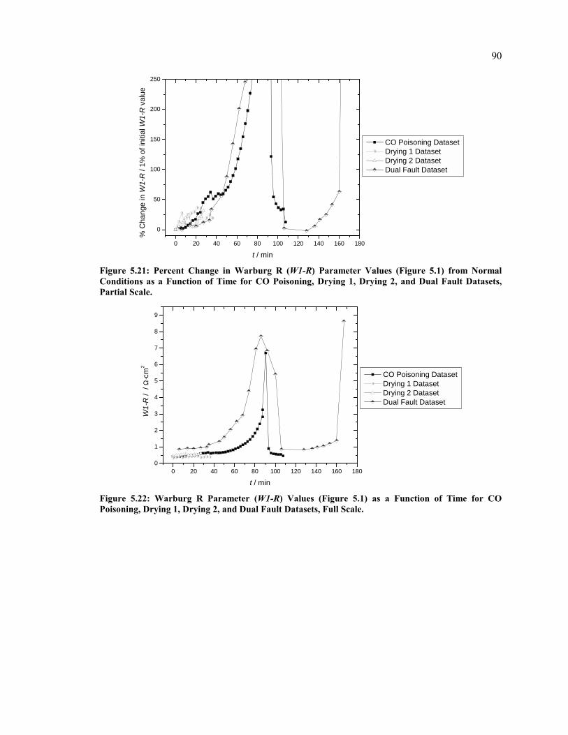
90

0 20 40 60 80 100 120 140 160 180

0

50

100

150

200

250


% C

hang

e in

W1-

R /

1% o

f ini

tial W

1-R

val

ue

t / min Figure 5.21: Percent Change in Warburg R (W1-R) Parameter Values (Figure 5.1) from Normal Conditions as a Function of Time for CO Poisoning, Drying 1, Drying 2, and Dual Fault Datasets, Partial Scale.

0 20 40 60 80 100 120 140 160 1800

1

2

3

4

5

6

7

8

9


W1-

R /

/ Ω

·cm

2

t / min Figure 5.22: Warburg R Parameter (W1-R) Values (Figure 5.1) as a Function of Time for CO Poisoning, Drying 1, Drying 2, and Dual Fault Datasets, Full Scale.

91

0 20 40 60 80 100 120 140 160 180

0

200

400

600

800

1000

1200

1400

1600


% C

hang

e in

W1-

R /

1% o

f ini

tial W

1-R

val

ue

t / min Figure 5.23: Percent Change in Warburg R (W1-R) Parameter Values (Figure 5.1) from Normal Conditions as a Function of Time for CO Poisoning, Drying 1, Drying 2, and Dual Fault Datasets, Full Scale.

The Warburg Element R parameter is the parameter that affects the width (effective

resistance) of the semicircle that it is used to express. It is discussed in Section 2.2.1.4.2.

For the CO poisoning dataset this parameter increases substantially as the voltage

decreases while for the Drying 1 and Drying 2 datasets, this parameter does increase as

the voltage decreases, but not to the same degree as it does with CO poisoning (Figure

5.19-Figure 5.23). The average fitting errors for the Warburg R parameters are 5.5% for

Drying 1, 7.6 % for Drying 2, and 3.3% for CO poisoning datasets respectively. A change

in the Warburg parameter with CO poisoning was not directly expected because the

Warburg impedance represents only diffusion. However, coupling between the diffusion

and electrochemical phenomena is subtle and might lead to the observed dependence of

the Warburg parameter on CO poisoning..

The Warburg R parameter increases as the voltage decreases for both the CO poisoning

and the drying sequences. The Warburg R parameter increases during flooding conditions

(Figure 5.19).

For the dual fault dataset, increases in the Warburg R parameter are quite consistent with

the Drying 1, Drying 2, and CO Poisoning for the respective fault conditions: 1000% for

92

CO poisoning and 30% for drying. There is a high (>106 %) fitting error for the dual fault

dataset points: t =60, 65, 70, 75,85, and 165 min. At these 6 points the average fitting

error for this parameter is 3000% while the average fitting error for this parameter for all

other times is 2.5%. This Warburg R parameter is likely somewhat sensitive to transient

behaviour.

5.3.2.2 Warburg φ Parameter

-- A B C D E F G H I0.000.020.040.060.080.100.120.140.160.180.200.220.240.260.280.300.320.340.36

W1

- φ

Flooding File Figure 5.24: Warburg φ Parameter (W1- φ) Values (Figure 5.1) for Flooding Dataset.

0 20 40 60 80 100 120 140 160 1800.000.020.040.060.080.100.120.140.160.180.200.220.240.260.280.300.320.340.36


War

burg

Ele

men

t W1

- φ

t / min Figure 5.25: Warburg φ Parameter (W1- φ) Values (Figure 5.1) as a Function of Time for CO Poisoning, Drying 1, Drying 2, and Dual Fault Datasets.

93

0 20 40 60 80 100 120 140 160 180-50

-40

-30

-20

-10

0

10

20

30

40

50


% C

hang

e in

W1-

φ / 1

% o

f ini

tial W

1-φ

valu

e

t / min

Figure 5.26: Percent Change in Warburg φ (W1- φ) Parameter Values (Figure 5.1) from Normal Conditions as a Function of Time for CO Poisoning, Drying 1, Drying 2, and Dual Fault Datasets.

The Warburg φ parameter does not track as strongly with the voltage as other parameters

do (Figure 5.24-Figure 5.26). The Drying 2 dataset Warburg φ parameter decreases as the

voltage decreases due to the fault. The Drying 1 dataset Warburg φ parameter does not

track as clearly, nor does the CO poisoning dataset Warburg φ parameter. There is a large

jump in the Warburg φ parameter in each of the datasets at the point where the fault stops

and recovery begins. The average fitting errors, for the Warburg φ parameter, are 6.6 %

for Drying 1, 16.8% for Drying 2, and 2.0 % for CO Poisoning datasets respectively. The

Warburg φ parameter does correlate with flooding behaviour (Figure 5.24).

The Warburg φ parameter does not substantially change with time or with decreases in

voltage for the dual fault dataset. There are spikes at the recovery points from drying and

CO poisoning, indicating a sensitivity to transience, as with many other parameters. The

average fitting error for the Warburg φ parameter is 8.4% for the dual fault dataset.

For a Warburg element to be descriptive of the impedance of diffusion, the φ parameter

needs to be approximately 0.5. For this model the Warburg φ parameter is closer to 0.3,

indicating that it is likely not directly associated with diffusion. One explanation for this

is the limited frequency range used for fitting with this models, we suspect that the

94

Warburg impedance affects the 1 kHz – 5 Hz frequency range but we are only using the

model to fit in the 50Hz-50kHz range because it cannot resolve the third impedance

feature, it is likely that the Warburg impedance plays a role in the low frequency behavior

and so, in limiting the frequency range of the fit, the ability to completely resolve the

Warburg impedance is diminished.

5.3.2.3 Warburg T Parameter

-- A B C D E F G H I0.00

0.05

0.10

0.15

0.20

0.25

0.30

0.35

0.40

W1-

T /

s

Flooding File Figure 5.27: Warburg T Parameter (W1-T) Values (Figure 5.1) for Flooding Dataset.

0 20 40 60 80 100 120 140 160 180

0.00

0.05

0.10

0.15

0.20

0.25

0.30

0.35

0.40


W1-

T / s

t / min Figure 5.28: Warburg T Parameter (W1-T) Values (Figure 5.1) as a Function of Time for CO Poisoning, Drying 1, Drying 2, and Dual Fault Datasets, Partial Scale.

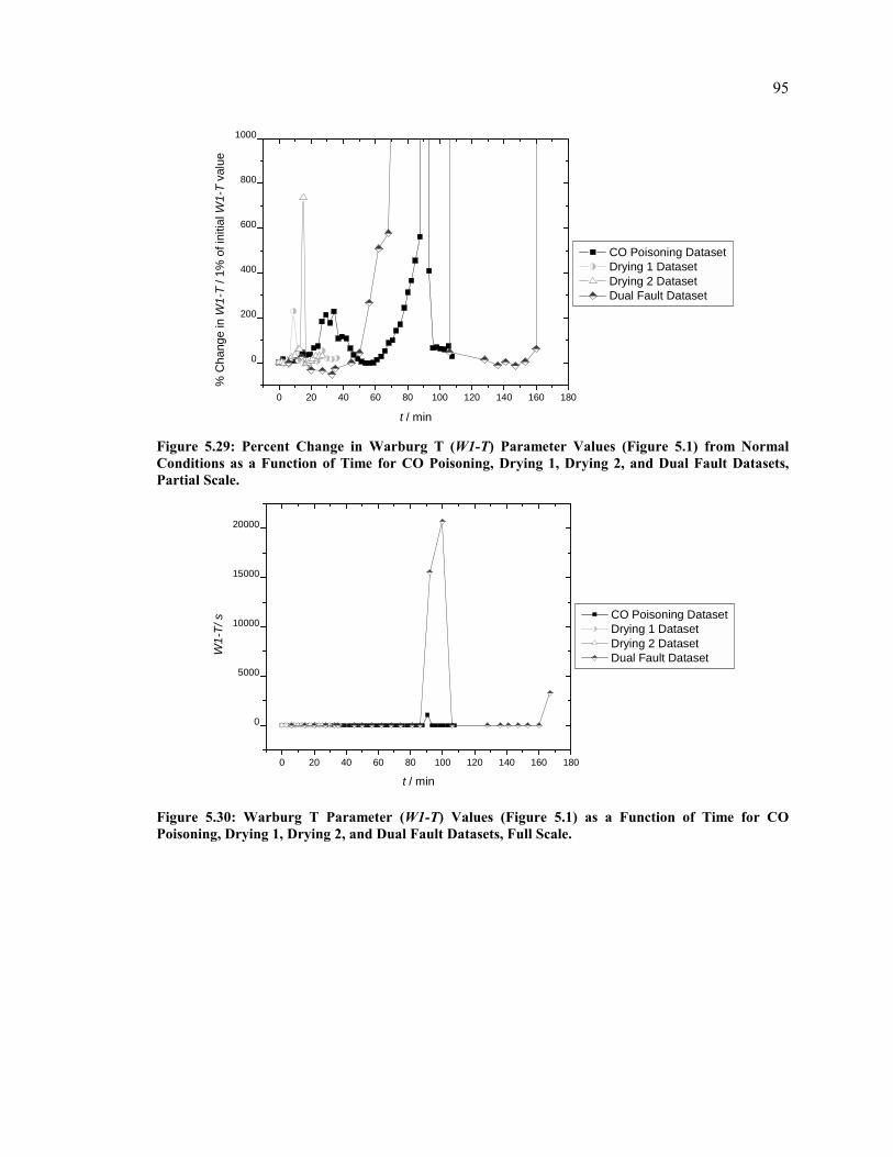
95

0 20 40 60 80 100 120 140 160 180

0

200

400

600

800

1000


% C

hang

e in

W1-

T / 1

% o

f ini

tial W

1-T

valu

e

t / min Figure 5.29: Percent Change in Warburg T (W1-T) Parameter Values (Figure 5.1) from Normal Conditions as a Function of Time for CO Poisoning, Drying 1, Drying 2, and Dual Fault Datasets, Partial Scale.

0 20 40 60 80 100 120 140 160 180

0

5000

10000

15000

20000


W1-

T/ s

t / min

Figure 5.30: Warburg T Parameter (W1-T) Values (Figure 5.1) as a Function of Time for CO Poisoning, Drying 1, Drying 2, and Dual Fault Datasets, Full Scale.

96

0 20 40 60 80 100 120 140 160 180

0.00E+000

5.00E+007

1.00E+008

1.50E+008

2.00E+008

2.50E+008

3.00E+008


% C

hang

e in

W1-

T / 1

% o

f ini

tial W

1-T

valu

e

t / min Figure 5.31: Percent Change in Warburg T (W1-T) Parameter Values (Figure 5.1) from Normal Conditions as a Function of Time for CO Poisoning, Drying 1, Drying 2, and Dual Fault Datasets, Full Scale.

For both drying and CO poisoning, the Warburg T parameter increases as the voltage

decreases with faults. For the CO poisoning dataset and Drying 2 dataset there is a sharp

increase in the value of the Warburg T parameter when the fuel cell recovers. This

parameter appears to be highly sensitive to the transience of impedance diagrams taken

during recovery from faults. The average fitting errors, for the Warburg T parameter, are

15.7% for Drying 1, 72.2% for Drying 2, and 15.1% for CO Poisoning (ignoring the CO

Poisoning error of >107% at t =90 min) respectively.

The Warburg T parameter does not significantly change with the decrease in voltage due

to drying for the dual fault dataset. This follows the behaviour of the drying datasets. The

CO poisoning sequence in the dual fault dataset behaves similarly to the CO poisoning

dataset with respect to the Warburg T parameter; it increases as the voltage decreases.

Again, as with other parameters there is a spike for impedance files acquired during

recovery from faults. The average fitting error for the Warburg T parameter for the dual

fault dataset is 9.1 × 106 % overall, and 29.1% excluding the data points from fault

recovery spectra.

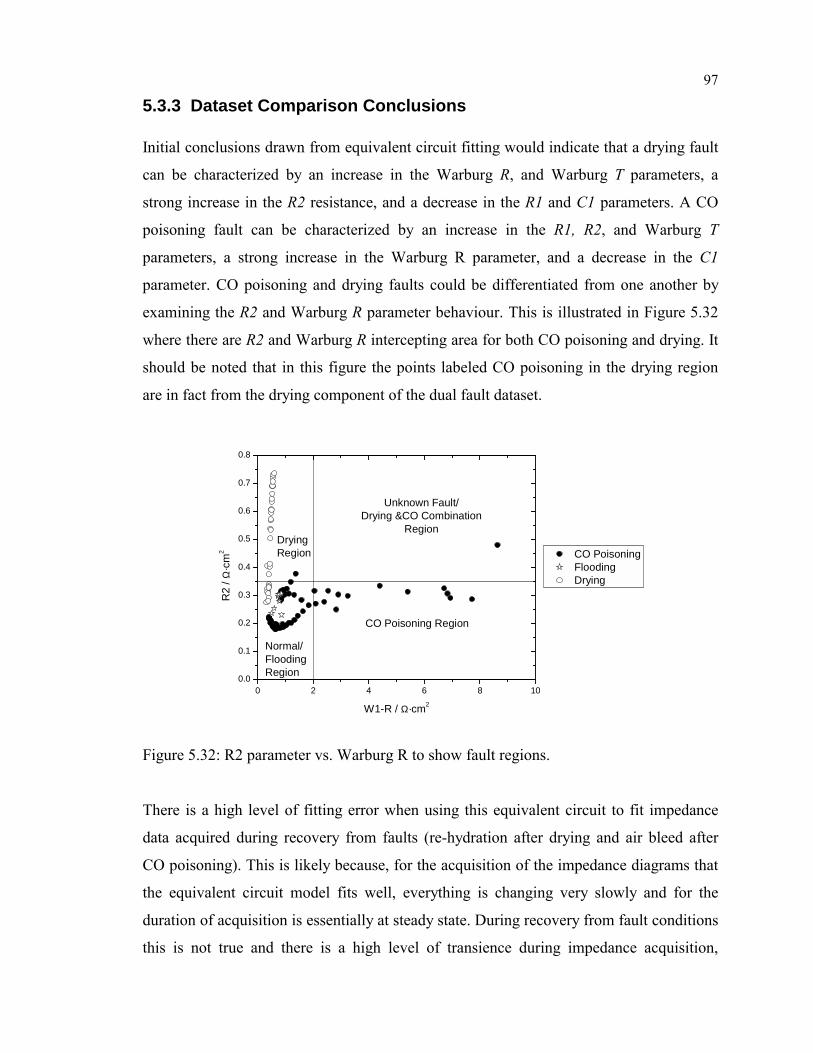
97

5.3.3 Dataset Comparison Conclusions Initial conclusions drawn from equivalent circuit fitting would indicate that a drying fault

can be characterized by an increase in the Warburg R, and Warburg T parameters, a

strong increase in the R2 resistance, and a decrease in the R1 and C1 parameters. A CO

poisoning fault can be characterized by an increase in the R1, R2, and Warburg T

parameters, a strong increase in the Warburg R parameter, and a decrease in the C1

parameter. CO poisoning and drying faults could be differentiated from one another by

examining the R2 and Warburg R parameter behaviour. This is illustrated in Figure 5.32

where there are R2 and Warburg R intercepting area for both CO poisoning and drying. It

should be noted that in this figure the points labeled CO poisoning in the drying region

are in fact from the drying component of the dual fault dataset.

0 2 4 6 8 100.0

0.1

0.2

0.3

0.4

0.5

0.6

0.7

0.8

CO Poisoning Flooding Drying

R2

/ Ω·c

m2

W1-R / Ω·cm2

Drying Region

CO Poisoning Region

Normal/FloodingRegion

Unknown Fault/Drying &CO Combination

Region

Figure 5.32: R2 parameter vs. Warburg R to show fault regions.

There is a high level of fitting error when using this equivalent circuit to fit impedance

data acquired during recovery from faults (re-hydration after drying and air bleed after

CO poisoning). This is likely because, for the acquisition of the impedance diagrams that

the equivalent circuit model fits well, everything is changing very slowly and for the

duration of acquisition is essentially at steady state. During recovery from fault conditions

this is not true and there is a high level of transience during impedance acquisition,

98

causing fittings with the equivalent circuit model to be less accurate particularly at lower

frequencies. In an integrated diagnostic device this fitting problem could cause false

positive readings for faults due to high levels of error in parameters. Alternatively, high

levels of error in fitting parameters could be used to diagnose highly transient conditions

in fuel cells.

Many of the equivalent circuit parameters change in a statistically significant manner as

the voltage decreases due to CO poisoning and drying faults. There are indications that

the rate of increase of parameters such as R2 and Warburg R could be used to

differentiate between CO poisoning and drying fault conditions. A problem with this type

of identification could be the possible effects of the rate and severity of performance

deterioration due to individual CO poisoning or drying events. Further study of drying

and CO poisoning events with differing rates and severity, with all other conditions

maintained constant, could help to solve this problem.

There is also concern about the fitting error. Equivalent circuit fitting using a CNLS

algorithm is very sensitive to starting parameters. When fitting the dual fault dataset it

was fit both in a scaled and un-scaled form. The results of these fittings were different

trends in parameters, essentially parameters which would not scale to be equivalent. This

is likely due to different initial parameters. Equivalent circuit fitting is also very sensitive

to transient conditions. It does not converge well for recovery datasets taken during air

bleed events during CO poisoning or re-hydration events during drying.

Information about fault status in fuel cells could be achieved using equivalent circuit

fitting with this model. This would likely be more appropriate for use in an off-board

setting as many frequencies need to be measured and there are often several iterations

required to converge to a “good fit”. Problems with unreliable fitting in transient

conditions could lead to false fault identification or identification of incorrect faults,

leading to incorrect response in an onboard control type setting, whereas in an off-board

setting they could be more easily used to identify transient conditions in the cell.

99

One of the advantages of equivalent circuit fitting is that information about fuel cell

material properties such as membrane resistivity, membrane dielectric permittivity, and

double-layer capacitance can be identified from model parameters. A better

understanding of the effects of a variety of fuel cell operating conditions could be used

not only as a diagnostic tool, but also as a basis for fuel cell and membrane design

improvement.

100

6 Single Frequency Analysis – First Circle and Drying Initially work was done, pursuant to equivalent circuit subtraction work (Section 4.3), to

identify the properties of the first semicircle of the impedance (particularly the resistance)

by following a single frequency. This work is also described in Ref. 3. The focus was on

the identification of drying conditions by monitoring a single frequency. The intent was

to develop fault condition cutoff points which could be used as either a part of a control

system to initiate humidification or as a safety device to shut down fuel cells prior to

membrane burn-through failure. The effect of noise and the possibility of false positive

drying fault identification were also investigated. Because much of this work required a

baseline for comparison, a variety of impedance spectra with similar conditions were

examined and averaged into “baseline data”. It should be noted that this baseline was

developed for comparative purposes only and does not necessarily reflect the “normal

operating conditions” of a fuel cell. To set actual cutoff points and for a better

understanding of the issue of noise, real baseline data would be needed.

6.1.1 First Circle RC Algorithm

A geometric algorithm was developed to estimate the electrolyte membrane resistance

from measured impedance data at frequencies above 1 kHz (the first semicircle

impedance feature). This algorithm uses the idea that the diameter of a semicircle,

centered on the horizontal axis and passing through the origin, can be determined

geometrically if the coordinates of a point on the arc are known (Figure 6.1).

Figure 6.1: Semicircle geometry used for drying fault algorithm

101

For a semicircle impedance signature the parallel resistance value is the diameter of the

semicircle. Using the experimental real and imaginary impedance values (Z’ and Z”) at a

given frequency (point P), the resistance (R) and capacitance (C) values for that signature

can be estimated by noting that triangles OPT and OQP in figure 1 are similar, so that:

')"()'( 22

ZZZR +=

Eq 6-1

and

RfC

top⋅=

π21

Eq 6-2

where ftop is the frequency at the center of the circle.

Although the capacitance can also track drying it is not as useful as the resistance for

several reasons: the additional parameter ftop required to calculate the capacitance is only

known approximately, and the percent increases of capacitance with drying are not as

high (a little less than 50 % of the resistance values).

6.2 Frequency Choice

To create a simple, effective on-board device, the optimal single frequency needs to be

chosen to identify the drying fault. The drying effect can be seen in the first semicircle

feature on the Nyquist impedance plot. This is in the 1 kHz and above frequency region

(Figure 6.2).

102

0.0 0.1 0.2 0.3 0.4 0.5 0.6 0.7 0.8 0.9 1.0 1.1 1.2 1.3 1.40.0

-0.1

-0.2

-0.3

-0.4

0.5 Hz1 Hz5 Hz

10 Hz50 Hz100 Hz

500 Hz1 kHz

5 kHz10 kHz

50 kHz

Im(Z

) / Ω

·cm

2

Re(Z) / Ω·cm2

Figure 6.2: Typical impedance spectra (Section 3.3) with Frequencies Identified

In order to choose the optimal frequency to follow to identify drying faults, measured

frequencies in the 1 kHz to 100 kHz region were examined. For spectra that were not

acquired to 100 kHz the highest frequency measured was used as the upper limit.

Frequencies below 1 kHz were not examined because they are heavily affected by second

feature; this is beyond the limits of the algorithm used and can lead to mistakes in

identification.

05

1015

2025

30

0.0

0.2

0.4

0.6

0.8

1.0

1.01.21.51.92.53.13.95.06.37.91012.515.819.925.131.639.850.163.179.4100

Frequency / kH

z

R /

Ω·c

m2

t / min

Figure 6.3: Change in membrane resistance, as estimated with the drying algorithm at individual frequencies, over time, gray bar at 5.0 kHz (Figure 3.10).

103

Figure 6.3 illustrates the change in resistance over time over a frequency range. It shows

that frequencies in the 1.2 kHz to 12 kHz range follow drying behavior well, while at

higher frequencies there is a steep drop in the magnitude of the estimated resistance. The

1.2 kHz to 12 kHz frequency range is also a logical choice because it is close to the top of

the semicircle, an advantage with the drying algorithm. A frequency of 5 kHz, the gray

bar on Figure 6.3, was chosen because of the magnitude of the increase of estimated

membrane resistance over time was significant compared to higher frequencies, and

because of concerns regarding feature overlap for lower frequencies.

6.3 Statistical Significance

In order to positively identify a drying fault, the change in estimated resistance needs to

be statistically significant compared to normal operating conditions. This means that the

normal variation in resistance during operation needs to be much lower than the variation

with drying.

The noise level in measured data is also important in determining the statistical

significance of the identification of the drying fault. The effect of noise, and the

maximum level of noise acceptable for the drying fault to be identified, has been

examined and is discussed below.

The statistical significance of the cutoff limit for drying in a variety of fuel cells needs to

be examined. It is not yet known if the membrane resistance that signifies “dry”

conditions is consistent between fuel cells.

6.3.1 Hypothetical Baseline

In order to create a hypothetical baseline, several spectra acquired at the conditions listed

below in the range of current densities of j = 0.05 to 0.5 A.cm2 were examined. The

typical normal operating conditions for the 4-cell stack or the single cell test assembly are

defined as follows:

104

• pfuel = poxidant = 30 psig,

• Tcell = 65 °C, Tfuel = 85 °C, Toxidant = 70 °C.

Using the first-circle algorithm to determine the resistance on “normal operation” data

gives average estimated resistivity of 0.25 Ω.cm2 per cell. The average variation in

normal conditions is about 15%.

6.3.2 Variation Due to Drying

Five sets of drying data were analyzed, with a focus on the Drying1 and Drying 2

datasets, to determine the degree of increase in the estimated membrane resistance with

drying. From this analysis it was determined that, estimating the resistance at a frequency

of 5 kHz, an increase of 50 % or more from a standard resistivity of 0.25 Ω⋅cm2 can

consistently indicate reversible drying, but drying can proceed to an increase of 150% or

more without incurring failure or irreversibility (Figure 6.4-Figure 6.5).

-2 0 2 4 6 8 10 12 14 16 18 20 22 24 26 28 30

0.60

0.65

0.70

0.75

0.80

0.85

0.90

t / min

R /

Ω·c

m2

140

160

180

200

220

240

260

% C

hange in R / 1%

of initial R value

Figure 6.4: Estimated membrane resistance (left) and percent increase in resistance above 0.25 ΩΩΩΩ.cm2 (right) with time (Drying 2 Dataset – Section 3.4.2).

105

0 10 20 30 40

0.32

0.34

0.36

0.38

0.40

0.42

0.44

0.46

0.48

0.50

0.52

0.54

t / min

R /

Ω.c

m2

30

40

50

60

70

80

90

100

110

% C

hange in R / 1%

of initial R value

Figure 6.5: Estimated membrane resistance (left) and percent increase in resistance above 0.25 ΩΩΩΩ.cm2 (right) with time (Drying 2 Dataset – Section 3.4.1).

Following the estimated membrane resistance gives a consistent indication of drying. For

this data 0.5 Ω⋅cm2 per cell, 100% above normal, would be an appropriate arbitrary cutoff

to indicate a drying fault in a fuel cell. For a control device 0.375 Ω⋅cm2 per cell, 50%

above normal, would be a good warning point to rectify temperature or humidification

problems.

The choice of cutoff to determine a drying fault could either be an arbitrary resistivity per

cell or (as above) a percentage above the normal operating resistivity. This choice would

depend on whether all fuel cells have the same characteristic resistivity per cell or if it

changes from stack to stack. If all fuel cells have the same characteristic resistivity and

change of resistivity with drying, then an arbitrary cutoff value scaled to stack size would

be an effective technique. If all fuel cell stacks have different resistivity and drying

characteristics then a sampling needs to be taken of individual or batches of stacks at

normal operating conditions and a percentage increase above normal for that stack would

be a better choice. In order to determine which method is preferable, tests need to be

performed on different stacks to determine manufacturing or type variations in the

measured membrane resistance.

106

Assuming the limits of a 50% increase as a warning, a 100% increase as a failure, and a a

single cell drying, the warning would show up as an increase in the overall stack

resistance of 12.5% in a 4 cell stack, 2.5% in a 20 cell stack and 0.5% in a 100 cell stack.

The failure would show up as in increase in the overall stack resistance of 25% for a 4

cell stack, 5% for a 20 cell stack, and 1% for a 100 cell stack.

6.3.3 Noise

This technique was designed with a final device, likely be a part of an onboard

diagnostics system, in mind. In that type of location noise levels are likely to be much

higher than those experienced in laboratory experiments. Because of this it is necessary to

determine the level of noise for experimental data after which this technique will no

longer maintain statistical significance. Noise tolerance is also of interest because a

smaller AC perturbation for impedance measurement would be preferable in a final

device because it would have less of an overall effect on the rest of the system. With

smaller amplitude perturbations the measured impedance data is generally noisier.

6.3.3.1 Noise Algorithm

A noise algorithm was developed to transform measured impedance data into “noisy”

impedance data. Noise was added at varying levels to the same files to make comparison

easier. The noise algorithm added noise randomly at each point to create the effect of

random noise in an application.

In order to generate the noise for a given frequency point, the magnitude of the

impedance (|Z|) at that frequency is multiplied by the “percentage” of noise applied

(%noise). This is then multiplied by a random number (nf); generated in Maple from a

normal distribution function with a standard deviation of 1.

nfnoiseZnoise ⋅⋅= %

Eq 6-3

107

Two noise values are generated for each frequency point and one is added to each the

measured real and imaginary impedance values at that frequency.

noiseZZ n += ''

Eq 6-4

and

noiseZZ n += ""

Eq 6-5

With this algorithm the noise is proportional to the magnitude of the impedance. For our

data this means that the noise will be larger at lower frequencies (Figure 6.6) because the

magnitude is larger. This makes sense for a variety or reasons including sample time.

This method has also been used by Orazem et al. for work with noise and impedance

data80.

0 5 10 15 20 25 300

-2

-4

-6

-8

-10

-12

-14Original Data

Im(Z

) / Ω

·cm

2

Re(Z) / Ω·cm20 5 10 15 20 25 30

0

-2

-4

-6

-8

-10

-12

-14

2% Noise Added

Im(Z

) / Ω

·cm

2

Re(Z) / Ω·cm2

0 5 10 15 20 25 300

-2

-4

-6

-8

-10

-12

-14

4% Noise Added

Im(Z

) / Ω

·cm

2

Re(Z) / Ω·cm20 5 10 15 20 25 30

0

-2

-4

-6

-8

-10

-12

-14

6% Noise Added

Im(Z

) / Ω

·cm

2

Re(Z) / Ω·cm2

0 5 10 15 20 25 300

-2

-4

-6

-8

-10

-12

-14

8% Noise Added

Im(Z

) / Ω

·cm

2

Re(Z) / Ω·cm20 5 10 15 20 25 30

0

-2

-4

-6

-8

-10

-12

-14

10% Noise Added

Im(Z

) / Ω

·cm

2

Re(Z) / Ω·cm2 Figure 6.6: Nyquist Plots of data with no noise, 2%, 4%, 6%, 8%, and 10% noise added (Conditions as in Figure 3.10, t = 15 min).

108

6.3.3.2 Noise Level Threshold

The noise level threshold is the level after which the error due to noise reduces the

statistical significance of the technique. To determine the probability of a false positive,

the difference (∆R) between the estimated resistance with noise (Rnoise) and without

(Rnoinoise) was taken for each impedance file in the Drying 2 dataset:

noisenonoise RRR −=∆

Eq 6-6

These differences were then used to determine a mean and standard deviation for the

distribution at each noise level.

To determine the probability that a false positive occurs, the distribution was considered

to be a normal distribution, consistent with the earlier assumptions in the development of

noisy data. The probability of a false positive was taken to be the probability of a

resistance above the cutoff resistance.

A 50% to 150% increase in estimated resistance indicates a drying fault. A false positive

will occur when the variation due to noise for normal operating conditions reaches this

level. The worst-case scenario would be when the normal operating condition is at the top

of the 15% variation and the cutoff for a drying fault is at 50% above normal conditions (

Figure 6.7:). In this case the 4% noise level would be the cutoff where a false positive

only occurs 1 out of 20 times instead of 1 out of 2 times as at 6% noise.

109

0 1.20E-04 4.07

57.89

41.96

141.16

95.22

166.5

137.75

150.96

199.13

0

50

100

150

200

250

0 2 4 6 8 10 12 14 16 18 20

Percent noise added

Prob

abili

ty th

at a

fals

e po

sitiv

e w

ill o

ccur

(%)

Figure 6.7: Probability that a false positive – (a reading of 0.375 ΩΩΩΩ⋅⋅⋅⋅cm2 ) will be achieved with a normal operating resistance of 0.2875 ΩΩΩΩ⋅⋅⋅⋅cm2 (15% above normal) – varying with noise level

Another scenario examined was when the considering the normal operating condition to

be at the top of 15% variation and the cutoff for a drying fault is at 100% above normal

conditions (Figure 6.8). In this case the 8% noise level would be the cutoff where a false

positive only occurs 7 out of 1000 times instead of 17 out of 100 times as at 12 % noise.

Figure 6.9 and Figure 6.10 illustrate the absolute error in R and the percent deviation

from normal conditions with the addition of differing levels of noise respectively.

110

0 0.00E+00 2.14E-05 1.12365 0.77269

17.8147 15.99044

79.42841

36.35573 34.87165

101.81465

0

20

40

60

80

100

120

0 2 4 6 8 10 12 14 16 18 20

Percent noise added

Prob

abili

ty th

at a

fals

e po

sitiv

e w

ill o

ccur

(%)

Figure 6.8: Probability that a false positive - a reading of 0.50 ΩΩΩΩ⋅⋅⋅⋅cm2 will be achieve with a normal operating resistance of 0.2875 ΩΩΩΩ⋅⋅⋅⋅cm2 (15% above normal) – varying with noise level

05

1015

2025

30

0

20

40

60

80

100

0

5

10

15

20

|Error| from Measured Average |Error| Average |Error|

|Err

or| (

% fr

om m

easu

red)

% Noise Added

t / min

Figure 6.9: Absolute error as a percentage of the estimated resistance values at 5 kHz vs. time and average absolute error with increasing noise levels for Drying 2 Dataset.

111

0 5 10 15 20

0

5

10

15

20

25

30

% D

evia

tion

from

est

. R

Noise Level (% of |Z|)

Figure 6.10: The average percent deviation from the estimated resistance vs. noise level for Drying 2 Data.

6.4 Summary

The drying fault can be reliably tracked, over time, by following the real and imaginary

components of the fuel cell impedance at 5 kHz, and estimating the membrane resistance.

Under the assumption of the hypothetical baseline conditions used, an increase of 50%

above normal resistance conditions indicates drying is occurring but increases of 150% or

more above normal can be attained without failure for our single cell fuel cell assembly.

To make a final decision on the universality of the cutoff resistance and frequency choice,

drying data from different fuel cell stacks and manufacturers should be studied. The work

with noise suggests that there is a fairly good tolerance for noise with this technique.

This method was pursued with the interest of gaining not only a method to track drying

but also a method to track membrane resistivity. It was later found that following

individual, un-manipulated, impedance parameters also track with faults. This is

discussed further in the following section.

112

7 Multi Frequency Analysis – All Faults

There is interest in developing techniques for onboard diagnostics and controls of running

fuel cells; a device that can quickly identify multiple faults and provide the correct

rectification or shut down in severe cases. For this purpose the acquisition and equivalent

circuit analysis of full impedance spectra is time consuming and requires complex

hardware and software to fit and monitor. The algorithm used for single frequency

analysis, though somewhat effective to monitor membrane properties, proved not to be

necessary to monitor fault conditions. There were also difficulties in differentiating

between drying and CO poisoning faults using a single frequency. Because of this multi-

frequency analysis (MFA) was investigated.

MFA, for the purpose of this work, is the monitoring and analysis of the impedance at

several individual frequencies to identify individual fault behaviour. This involves

measuring the impedance at several frequencies and monitoring to ensure that fault

thresholds are not reached. Ideally in an onboard device there would be a fault threshold

and a warning threshold, both integrated into the fuel cell control system. If the warning

threshold for a known fault is passed then the fuel cell control system could adjust

humidification or air bleed in order to rectify the problem. If the fault were to persist to

the fault threshold then the fuel cell could be shut down before irreparable damage was

done.

In an onboard situation the frequencies chosen would be continuously monitored. For the

purposes of this analysis individual frequency data from measured impedance spectra

were extracted and compared at each frequency as no hardware to continuously monitor

several frequencies was available.

It should be noted that parameter thresholds are not intensively discussed in this section

because there are discrepancies between “normal operating conditions” for the fault

datasets. These discrepancies are likely due to the differing conditions required to

113

produce different fault conditions and the fact that impedance spectra were not

continuously acquired from an initial hydrated state in the case of the drying faults.

7.1 Frequency choice

There are several factors influencing the choice of frequencies for MFA. Because time of

acquisition is important in MFA, higher frequencies are more appealing. Also there are

the physical limitations of the measurement device to consider, measurements at too high

or too low a frequency can be susceptible to noise or measurement artifacts. The most

important factor in choosing the frequencies is that they be able to represent sufficient

impedance information to enable the fault conditions to be distinguished (particularly

between CO poisoning and Drying).

5 kHz (at the apex of the first semi-circle feature), 500 Hz (between the first and second

semicircle features), and 50 Hz (on the start of the second semi-circle feature), were

chosen as the three frequencies for the analysis of impedance fault data in this work

(Figure 7.1). Three frequencies were chosen because two frequencies were insufficient to

represent the impedance data: the spacing of the semicircles, and size of the second

semicircle in relation to the first can be identified with three frequencies but not with two.

The three frequencies chosen were shown to give the best distinction between CO

poisoning and drying of the 11 frequencies attempted. The real and imaginary parts of the

impedance as well as the phase and magnitude for drying and CO poisoning data were

compared at 0.5 Hz, 1 Hz, 5 Hz, 10 Hz, 50 Hz, 100 Hz, 500 Hz, 1 kHz, 5 kHz, 10 kHz,

and 50 kHz. From this comparison, and pursuant to the single frequency work in Section

6, 5000 Hz, 500 Hz, and 50 Hz were chosen.

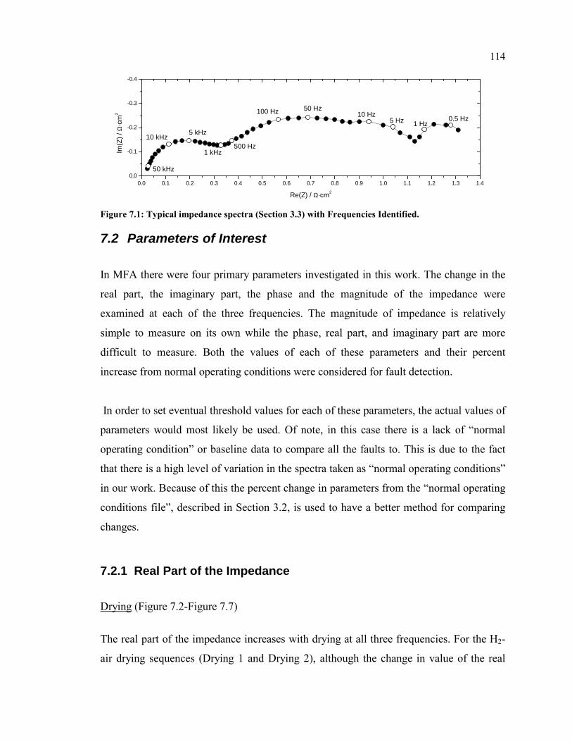
114

0.0 0.1 0.2 0.3 0.4 0.5 0.6 0.7 0.8 0.9 1.0 1.1 1.2 1.3 1.40.0

-0.1

-0.2

-0.3

-0.4

0.5 Hz1 Hz5 Hz

10 Hz50 Hz100 Hz

500 Hz1 kHz

5 kHz10 kHz

50 kHz

Im(Z

) / Ω

·cm

2

Re(Z) / Ω·cm2

Figure 7.1: Typical impedance spectra (Section 3.3) with Frequencies Identified.

7.2 Parameters of Interest

In MFA there were four primary parameters investigated in this work. The change in the

real part, the imaginary part, the phase and the magnitude of the impedance were

examined at each of the three frequencies. The magnitude of impedance is relatively

simple to measure on its own while the phase, real part, and imaginary part are more

difficult to measure. Both the values of each of these parameters and their percent

increase from normal operating conditions were considered for fault detection.

In order to set eventual threshold values for each of these parameters, the actual values of

parameters would most likely be used. Of note, in this case there is a lack of “normal

operating condition” or baseline data to compare all the faults to. This is due to the fact

that there is a high level of variation in the spectra taken as “normal operating conditions”

in our work. Because of this the percent change in parameters from the “normal operating

conditions file”, described in Section 3.2, is used to have a better method for comparing

changes.

7.2.1 Real Part of the Impedance

Drying (Figure 7.2-Figure 7.7)

The real part of the impedance increases with drying at all three frequencies. For the H2-

air drying sequences (Drying 1 and Drying 2), although the change in value of the real

115

part of the impedance is different for the three frequencies, the percent increase in Re(Z)

remains approximately 40% at each frequency. The drying data acquired with reformate

show a similar result except that the percent increase is larger at 50 Hz than at 500 Hz and

5000 Hz. This may be due to incomplete recovery from CO poisoning or could be a

characteristic of drying with reformate.

CO Poisoning (Figure 7.2-Figure 7.7)

The real part of the impedance increases with CO poisoning at all three frequencies, but

increases more steeply at 500 Hz than at 5000 Hz and even more steeply at 50 Hz than at

500 Hz. The percent change also increases as frequency decreases.

Flooding (Figure 7.8)

The real part of the impedance does not change significantly with flooding in this

frequency range.

Variation of Gas Composition (Figure 7.9-Figure 7.11)

The real part of the impedance does not vary significantly at 500 Hz or 5000 Hz with

changing gas compositions or current density. At 50 Hz the real part of the impedance is

slightly higher for datasets acquired with reformate instead of hydrogen but not in a

manner that could be interpreted as statistically significant. The real part of the

impedance decreases slightly as current density increases.

Summary

Drying and CO poisoning could be differentiated using the real part of the impedance

because drying (both with hydrogen and reformate) shows a larger increase in the real

part of the impedance at 5000 Hz than CO poisoning. Drying with hydrogen also

maintains a fairly similar percentage increase at all three frequencies (40%). Drying with

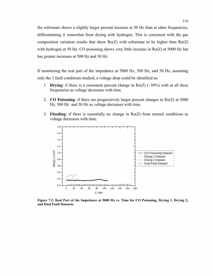
116

the reformate shows a slightly larger percent increase at 50 Hz than at other frequencies,

differentiating it somewhat from drying with hydrogen. This is consistent with the gas

composition variation results that show Re(Z) with reformate to be higher than Re(Z)

with hydrogen at 50 Hz. CO poisoning shows very little increase in Re(Z) at 5000 Hz but

has greater increases at 500 Hz and 50 Hz.

If monitoring the real part of the impedance at 5000 Hz, 500 Hz, and 50 Hz, assuming

only the 3 fault conditions studied, a voltage drop could be identified as:

1. Drying: if there is a consistent percent change in Re(Z) (~50%) with at all three frequencies as voltage decreases with time.

2. CO Poisoning: if there are progressively larger percent changes in Re(Z) at 5000

Hz, 500 Hz and 50 Hz as voltage decreases with time.

3. Flooding: if there is essentially no change in Re(Z) from normal conditions as voltage decreases with time.

0 20 40 60 80 100 120 140 160 1800.0

0.2

0.4

0.6

0.8

1.0

1.2

1.4

1.6

1.8


Re(

Z) /

Ω·c

m2

t / min Figure 7.2: Real Part of the Impedance at 5000 Hz vs. Time for CO Poisoning, Drying 1, Drying 2, and Dual Fault Datasets.

117

0 20 40 60 80 100 120 140 160 180-20

0

20

40

60

80

100

120

140

160

180


% C

hang

e in

Re(

Z) /

1%

of i

nitia

l Re(

Z) v

alue

t / min

Figure 7.3: Percent Change in the Real Part of the Impedance at 5000 Hz vs. Time for CO Poisoning, Drying 1, Drying 2, and Dual Fault Datasets.

0 20 40 60 80 100 120 140 160 1800.0

0.2

0.4

0.6

0.8

1.0

1.2

1.4

1.6

1.8


Re(

Z) /

Ω·c

m2

t / min

Figure 7.4: Real Part of the Impedance at 500 Hz vs. Time for CO Poisoning, Drying 1, Drying 2, and Dual Fault Datasets.

118

0 20 40 60 80 100 120 140 160 180-20

0

20

40

60

80

100

120

140

160

180


% C

hang

e in

Re(

Z) /

1%

of i

nitia

l Re(

Z) v

alue

t / min


0 20 40 60 80 100 120 140 160 1800.0

0.2

0.4

0.6

0.8

1.0

1.2

1.4

1.6

1.8


Re(

Z) /

Ω·c

m2

t / min

Figure 7.6: Real Part of the Impedance at 50 Hz vs. Time for CO Poisoning, Drying 1, Drying 2, and Dual Fault Datasets.

119

0 20 40 60 80 100 120 140 160 180-20

0

20

40

60

80

100

120

140

160

180


% C

hang

e in

Re(

Z) /

1%

of i

nitia

l Re(

Z) v

alue

t / min


-- A B C D E F G H I

0.2

0.4

0.6

0.8

1.0

1.2

1.4

1.6

1.8

5000 Hz 500 Hz 50 Hz 5 Hz 0.5 Hz

Re(

Z) /

Ω·c

m2

Flooding File

Figure 7.8: Real Part of the Impedance for Flooding Data Files at 5000 Hz, 500 Hz, 50 Hz, 5 Hz, and 0.5 Hz.

120

0.05 0.10 0.15 0.20 0.25 0.300.1

0.2

0.3

0.4

0.5

0.6

0.7

0.8

0.9

1.0

H2-O2 H2-60% O2 H2-Air Ref-60% O2 Ref-Air

Cel

l 1: R

e(Z)

/ Ω

·cm

2

j / A·cm-2

Figure 7.9: Real Part of the Impedance at 5000 Hz vs. Current Density for H2-O2, H2-60% O2 , H2-Air, Ref – 60% O2 , and Ref-Air Datasets.

0.05 0.10 0.15 0.20 0.25 0.300.1

0.2

0.3

0.4

0.5

0.6

0.7

0.8

0.9

1.0


Cel

l 1: R

e(Z)

/ Ω

·cm

2

j / A·cm-2


121

0.05 0.10 0.15 0.20 0.25 0.300.1

0.2

0.3

0.4

0.5

0.6

0.7

0.8

0.9

1.0


Cel

l 1: R

e(Z)

/ Ω

·cm

2

j / A·cm-2


7.2.2 Imaginary part of the Impedance


For the H2 –Air datasets, Drying 1 and Drying2, the absolute imaginary part of the

impedance increases with drying behaviour at 5000 Hz and 500 Hz and there is little

change at 50 Hz. The percent change in the absolute imaginary part of the impedance is

approximately 50 % at 5000 Hz, 30% at 500 Hz, and 25% at 50 Hz.

For the dual fault dataset the magnitude of the imaginary part of the impedance increases

with CO poisoning behaviour, with greater increases at 500 Hz and 50 Hz than at 5000

Hz. The percent change in the absolute imaginary part of the impedance increases as

frequency decreases.

The discrepancy between the behaviour of the imaginary part for the Drying 1 and Drying

2 datasets and the dual fault dataset is probably due to the affect of the reformate. The

absolute imaginary part of the impedance at 50 Hz is greater for the reformate air

combination (Figure 7.21) than for all the other gas combinations; this could be affecting

the drying data behaviour in the dual fault dataset.

122


The absolute imaginary part of the impedance increases with CO poisoning. The percent

change in the absolute imaginary part of the impedance increases as frequency decreases.


The imaginary part of the impedance does not change significantly with flooding at 5000,

500, or 50 Hz. It does however change significantly with flooding behaviour at 0.5 Hz

(Figure 7.18).


At 5000 Hz there is very little variation in the magnitude of the imaginary part of the

impedance with gas composition or current density. At 500 Hz the magnitude of the

imaginary part of the impedance for datasets acquired with reformate was larger than

|Im(Z)| for datasets acquired with hydrogen. There was very little change with current

density. At 50 Hz the |Im(Z)| values for the dataset acquired with reformate-air were

slightly larger than the others, which were all fairly similar. There was a decrease in

|Im(Z)| with increasing current density.

Summary

The imaginary part of the impedance is less useful than the real part of the impedance to

differentiate between CO poisoning and drying conditions. It increases with decreasing

frequency for drying with hydrogen but not for drying with reformate. Im(Z) decreases

with decreasing frequency for CO poisoning and drying with reformate. This makes it

difficult to differentiate between the two phenomena using the imaginary part of the

impedance.

123

If monitoring the imaginary part of the impedance at 5000 Hz, 500 Hz, 50 Hz, and 0.5 Hz

assuming only the 3 fault conditions studied, a voltage drop could be identified as:

1. Drying: if there is a fairly consistent (within 50%) percent change in |Im(Z)| at all three frequencies as voltage decreases with time.

2. CO Poisoning: if there are progressively larger percent changes in |Im(Z)| at 5000

Hz, 500 Hz and 50 Hz, with a relatively high percent in crease (>200%) at 50 Hz as voltage decreases with time.

3. Flooding: if there is essentially no change in |Im(Z)| from normal conditions at

5000, 500, and 50 Hz, but there are significant changes in |Im(Z)| at 0.5 Hz as voltage decreases with time.

0 20 40 60 80 100 120 140 160 180-1.1

-1.0

-0.9

-0.8

-0.7

-0.6

-0.5

-0.4

-0.3

-0.2

-0.1

0.0


Im(Z

) / Ω

·cm

2

t / min

Figure 7.12: Imaginary Part of the Impedance at 5000 Hz vs. Time for CO Poisoning, Drying 1, Drying 2, and Dual Fault Datasets.

124

0 20 40 60 80 100 120 140 160 180-50

0

50

100

150

200

250

300

350

400

450


% C

hang

e in

Im(Z

) /

1% o

f ini

tial I

m(Z

) val

ue

t / min

Figure 7.13: Percent Change in the Imaginary Part of the Impedance at 5000 Hz vs. Time for CO Poisoning, Drying 1, Drying 2, and Dual Fault Datasets.

0 20 40 60 80 100 120 140 160 180

-1.0

-0.8

-0.6

-0.4

-0.2

0.0


Im(Z

) / Ω

·cm

2

t / min


125

0 20 40 60 80 100 120 140 160 180-50

0

50

100

150

200

250

300

350

400

450


% C

hang

e in

Im(Z

) /

1% o

f ini

tial I

m(Z

) val

ue

t / min Figure 7.15: Percent Change in the Imaginary Part of the Impedance at 500 Hz vs. Time for CO Poisoning, Drying 1, Drying 2, and Dual Fault Datasets.

0 20 40 60 80 100 120 140 160 180-1.1

-1.0

-0.9

-0.8

-0.7

-0.6

-0.5

-0.4

-0.3

-0.2

-0.1

0.0


Im(Z

) / Ω

·cm

2

t / min


126

0 20 40 60 80 100 120 140 160 180-50

0

50

100

150

200

250

300

350

400

450


% C

hang

e in

Im(Z

) /

1% o

f ini

tial I

m(Z

) val

ue

t / min

Figure 7.17: Percent Change in the Imaginary Part of the Impedance at 50 Hz vs. Time for CO Poisoning, Drying 1, Drying 2, and Dual Fault Datasets.

-- A B C D E F G H I-1.1

-1.0

-0.9

-0.8

-0.7

-0.6

-0.5

-0.4

-0.3

-0.2

-0.1

0.0

5000 Hz 500 Hz 50 Hz 5 Hz 0.5 Hz

Im(Z

) / Ω

·cm

2

Flooding File

Figure 7.18: Imaginary Part of the Impedance for Flooding Data Files at 5000 Hz, 500 Hz, 50 Hz, 5 Hz, and 0.5 Hz.

127

0.05 0.10 0.15 0.20 0.25 0.30-0.50

-0.45

-0.40

-0.35

-0.30

-0.25

-0.20

-0.15

-0.10

-0.05


Cel

l 1: I

m(Z

) / Ω

·cm

2

j / A·cm-2

Figure 7.19: Imaginary Part of the Impedance at 5000 Hz vs. Current Density for H2-O2, H2-60% O2 , H2-Air, Ref – 60% O2 , and Ref-Air Datasets.

0.05 0.10 0.15 0.20 0.25 0.30-0.50

-0.45

-0.40

-0.35

-0.30

-0.25

-0.20

-0.15

-0.10

-0.05


Cel

l 1: I

m(Z

) / Ω

·cm

2

j / A·cm-2


128

0.05 0.10 0.15 0.20 0.25 0.30-0.50

-0.45

-0.40

-0.35

-0.30

-0.25

-0.20

-0.15

-0.10

-0.05


Cel

l 1: I

m(Z

) / Ω

·cm

2

j / A·cm-2


7.2.3 Phase


The phase of the impedance does not change substantially with drying using either

hydrogen or reformate at all three frequencies. The percent change in the phase remains

below 10 % for all three frequencies as well.


The absolute phase of the impedance increases with CO poisoning. The percent change in

the absolute phase of the impedance is greatest at 50 Hz (>50%).


Flooding can be characterized by very little change in phase at 5000 Hz and an increase

in the absolute phase of the impedance at 500 and 50 Hz (>10 degrees).

129


At 5000 Hz and 500 Hz the absolute phase for datasets acquired with reformate is

approximately 5 degrees larger than that of datasets acquired with hydrogen. At 5000 Hz,

the magnitude of the phase does not change with current density, but at 500 Hz the

magnitude of the phase increases as current density decreases. At 50 Hz the phase for the

reformate-air and hydrogen-air datasets is about 5 degrees smaller than the phase for the

other datasets. The phase at 50 Hz decreases with decreasing current density. Several

other datasets would need to be acquired and analyzed to evaluate these trends with any

kind of accuracy.

Summary

The phase does not change significantly with drying (both with hydrogen and reformate)

at all three frequencies. The phase does change significantly with CO poisoning,

particularly at 500 Hz and 50 Hz. It is of some concern that the phase changes

significantly with current density at 50 Hz. It would likely be best to monitor the phase at

500 Hz, then if there is a change it is likely CO poisoning.

There is some difficulty differentiating between CO poisoning and flooding with the

phase of the impedance. If monitoring the phase the impedance at 5000 Hz, 500 Hz, and

50 Hz assuming only the 3 fault conditions studied, a voltage drop could be identified as:

1. Drying: if there is very little (<10 %) change in the phase of the impedance at 5000, 500, and 50 Hz as voltage decreases with time.

2. CO Poisoning or Flooding: if there relatively low (< 20 %) percent change in the

phase of the impedance at 5000 Hz and larger increases in the percent change in the phase of the impedance at 500 and 50 Hz.

130

0 20 40 60 80 100 120 140 160 1800

10

20

30

40

50

60

70

80

90


φ / d

egre

es

t / min

Figure 7.22: Phase of the Impedance at 5000 Hz vs. Time for CO Poisoning, Drying 1, Drying 2, and Dual Fault Datasets.

0 20 40 60 80 100 120 140 160 180-20

0

20

40

60

80

100

120


% C

hang

e in

φ

/ 1%

of i

nitia

l φ v

alue

t / min

Figure 7.23: Percent Change in the Phase of the Impedance at 5000 Hz vs. Time for CO Poisoning, Drying 1, Drying 2, and Dual Fault Datasets.

131

0 20 40 60 80 100 120 140 160 1800

10

20

30

40

50

60

70

80

90


φ / d

egre

es

t / min


0 20 40 60 80 100 120 140 160 180-20

0

20

40

60

80

100

120


% C

hang

e in

φ

/ 1%

of i

nitia

l φ v

alue

t / min


132

0 20 40 60 80 100 120 140 160 1800

10

20

30

40

50

60

70

80

90


φ / d

egre

es

t / min


0 20 40 60 80 100 120 140 160 180-20

0

20

40

60

80

100

120


% C

hang

e in

φ

/ 1%

of i

nitia

l φ v

alue

Time (min)


133

-- A B C D E F G H I0

10

20

30

40

50

60

70

80

90

5000 Hz 500 Hz 50 Hz 5 Hz 0.5 Hz

φ (d

egre

es)

Flooding Files

Figure 7.28: Phase of the Impedance for Flooding Data Files at 5000 Hz, 500 Hz, 50 Hz, 5 Hz, and 0.5 Hz.

0.05 0.10 0.15 0.20 0.25 0.300

10

20

30

40

50


Cel

l 1: φ

/ de

gree

s

j / A·cm-2

Figure 7.29: Phase of the Impedance at 5000 Hz vs. Current Density for H2-O2, H2-60% O2 , H2-Air, Ref – 60% O2 , and Ref-Air Datasets.

134

0.05 0.10 0.15 0.20 0.25 0.300

10

20

30

40

50


Cel

l 1: φ

/ de

gree

s

j / A·cm-2


0.05 0.10 0.15 0.20 0.25 0.300

10

20

30

40

50


Cel

l 1: φ

/ de

gree

s

j / A·cm-2


135

7.2.4 Magnitude

The magnitude of the impedance is relatively the easiest to measure of the parameters

examined in this section.


Although the actual change in magnitude is different at each frequency for drying (both

with hydrogen and reformate) the percent change in magnitude remains relatively fixed

for all three frequencies at approximately 50%.


The magnitude of the impedance increases with CO Poisoning. The percent change in the

magnitude of the impedance due to CO poisoning increases with decreasing frequency.


The magnitude of the impedance does not change significantly (<10 %) with flooding at

5000, 500, or 50 Hz.

Variation in Gas Composition (Figure 7.39-Figure 7.41)

There is very little change in the magnitude of the impedance at 5000 Hz and 500 Hz due

to gas composition or current density. At 50 Hz the magnitude of the impedance is

slightly larger for the dataset acquired with reformate, and the magnitude decreases with

increasing current density.

Summary

For drying conditions, both with reformate and hydrogen, the percent change in the

magnitude from normal conditions remains fairly constant (~50%) at all three frequencies

136

while, for CO poisoning conditions, the percent change in the magnitude increases as

frequency decreases. There is very little change in the magnitude of the impedance

(>10%) with flooding.

If monitoring the magnitude of the impedance at 5000 Hz, 500 Hz, and 50 Hz, assuming

only the 3 fault conditions studied, a voltage drop could be identified as:

1. Drying: if there is a consistent percent increase of ~50% in |Z| with at all three frequencies as voltage decreases with time.

2. CO Poisoning: if there are progressively larger percent increases in |Z| at 5000

Hz, 500 Hz and 50 Hz as voltage decreases with time.

3. Flooding: if there is essentially no change in |Z| from normal conditions as voltage decreases with time.

137

0 20 40 60 80 100 120 140 160 1800.0

0.2

0.4

0.6

0.8

1.0

1.2

1.4

1.6

1.8


|Z| /

Ω·c

m2

t / min

Figure 7.32: Magnitude of the Impedance at 5000 Hz vs. Time for CO Poisoning, Drying 1, Drying 2, and Dual Fault Datasets.

0 20 40 60 80 100 120 140 160 180-50

0

50

100

150

200

250


% C

hang

e in

|Z|

/ 1%

of i

nitia

l |Z|

val

ue

t / min

Figure 7.33: Percent Change in the Magnitude of the Impedance at 5000 Hz vs. Time for CO Poisoning, Drying 1, Drying 2, and Dual Fault Datasets.

138

0 20 40 60 80 100 120 140 160 1800.0

0.2

0.4

0.6

0.8

1.0

1.2

1.4

1.6

1.8


|Z| /

Ω·c

m2

t / min


0 20 40 60 80 100 120 140 160 180-50

0

50

100

150

200

250


% C

hang

e in

|Z|

/ 1%

of i

nitia

l |Z|

val

ue

t / min


139

0 20 40 60 80 100 120 140 160 1800.0

0.2

0.4

0.6

0.8

1.0

1.2

1.4

1.6

1.8


|Z| /

Ω·c

m2

t / min


0 20 40 60 80 100 120 140 160 180-50

0

50

100

150

200

250


% C

hang

e in

|Z|

/ 1%

of i

nitia

l |Z|

val

ue

t / min


140

-- A B C D E F G H I0.0

0.2

0.4

0.6

0.8

1.0

1.2

1.4

1.6

1.8

5000 Hz 500 Hz 50 Hz 5 Hz 0.5 Hz

|Z|

/ Ω·c

m2

Flooding File

Figure 7.38: Magnitude of the Impedance for Flooding Data Files at 5000 Hz, 500 Hz, 50 Hz, 5 Hz, and 0.5 Hz.

0.05 0.10 0.15 0.20 0.25 0.300.2

0.3

0.4

0.5

0.6

0.7

0.8

0.9

1.0


Cel

l 1: |

Z| /

Ω·c

m2

j / A·cm-2

Figure 7.39: Magnitude of the Impedance at 5000 Hz vs. Current Density for H2-O2, H2-60% O2 , H2-Air, Ref – 60% O2 , and Ref-Air Datasets.

141

0.05 0.10 0.15 0.20 0.25 0.300.2

0.3

0.4

0.5

0.6

0.7

0.8

0.9

1.0


Cel

l 1: |

Z| /

Ω·c

m2

j / A·cm-2


0.05 0.10 0.15 0.20 0.25 0.300.2

0.3

0.4

0.5

0.6

0.7

0.8

0.9

1.0


Cel

l 1: |

Z| /

Ω·c

m2

j / A·cm-2


142

7.2.5 Slopes

To examine the interrelation between the three frequencies and how this is affected by

fault conditions, threes slopes were analyzed. Each slope was calculated as follows, as

illustrated in Eq 7-1, Eq 7-2, and Eq 7-3:

0)Re(0)Im(

15000

5000

−−

==

=

ω

ω

ZZ

Slope

Eq 7-1

)Re()Re()Im()Im(

25000500

5000500

==

==

−−

=ωω

ωω

ZZZZ

Slope

Eq 7-2

)Re()Re()Im()Im(

350050

50050

==

==

−−

=ωω

ωω

ZZZZ

Slope

Eq 7-3

0.0 0.1 0.2 0.3 0.4 0.5 0.6 0.7 0.8 0.9 1.0 1.1 1.2 1.3 1.40.0

-0.1

-0.2

-0.3

-0.4

50 Hz

500 Hz

5000 Hz Slope 3Slope 2

Slope 1Im(Z

) / Ω

·cm

2

Re(Z) / Ω·cm2

Figure 7.42:Typical Impedance Spectra with slopes 1,2, and 3 illustrated


Slopes 1 and 3 do not change appreciably with drying conditions with either hydrogen or

reformate. Slope 2 does change with drying (approximately 50 % increase in magnitude)

143

but not as significantly as CO poisoning does. Slopes 2 and 3 are positive for drying

conditions, indicative of the characteristic shape of drying impedance data with a larger

first semicircle feature.


All three slopes change significantly with CO poisoning. Slopes 1 and 3 decrease as CO

poisoning increases and Slope 2 increases then decreases before recovery. Those slopes

that did not begin negative (Slopes 2 and 3) became negative as CO poisoning increased

indicating an increase in the height of the second semicircle feature.

Flooding (Figure 7.43-Figure 7.54)

Slope 1 and Slope 2 do not change significantly with flooding conditions. Slope 3 varied

with flooding, but not consistently. It should be noted that Slope 3 was consistently

negative for flooding behaviour, indicating an increase in the height of the second

semicircle feature.

Variation in Gas Composition (Figure 7.43-Figure 7.54)

There is some variation in the slopes with gas composition but not a significant amount.

There is a decrease in all three slopes as current density decreases.

Summary

If monitoring the real part and imaginary part of the impedance at 5000 Hz, 500 Hz, and

50 Hz, assuming only the 3 fault conditions studied, a voltage drop could be identified by

the slope 1, slope 2, and slope 3 behaviour as:

1. Drying: if Slope 1 is negative and its magnitude changes ~10 %, Slope 2 is positive and its magnitude does not change significantly, and Slope 3 is positive and its magnitude changes ~25 %.

144

2. CO Poisoning: if Slope 1 is negative and its magnitude changes with, Slope 2 is becomes negative and the percent change of its magnitude is significant ~50%, and Slope 3 becomes negative and the percent change of its magnitude is large ~300%,.

3. Flooding: if Slope 1 is negative and does not change significantly, Slope 2 is positive and its magnitude does not change significantly, and Slope 3 is negative.

0 20 40 60 80 100 120 140 160 180-5.0

-4.5

-4.0

-3.5

-3.0

-2.5

-2.0

-1.5

-1.0


Slo

pe 1

t / min

Figure 7.43: Slope 1 Values vs. Time for CO Poisoning, Drying 1, Drying 2, and Dual Fault Datasets.

0 20 40 60 80 100 120 140 160 180

-40

-20

0

20

40

60

80

100

120

140

160


% C

hang

e in

Slo

pe 1

/ 1%

of i

nitia

l Slo

pe 1

val

ue

t / min

Figure 7.44: Percent Change in Slope 1 Values vs. Time for CO Poisoning, Drying 1, Drying 2, and Dual Fault Datasets.

145

A B C D E F G H I-5.0

-4.5

-4.0

-3.5

-3.0

-2.5

-2.0

-1.5

-1.0

Slo

pe 1

Flooding File

Figure 7.45: Flooding Dataset Slope 1 Values.

0.05 0.10 0.15 0.20 0.25 0.30

-0.55

-0.50

-0.45

-0.40

-0.35

-0.30

-0.25

-0.20

-0.15

-0.10

-0.05


Cel

l 1: S

lope

1

j / A·cm-2

Figure 7.46: Slope 1 Values vs. Current Density for H2-O2, H2-60% O2 , H2-Air, Ref – 60% O2 , and Ref-Air Datasets.

146

0 20 40 60 80 100 120 140 160 180-0.8

-0.7

-0.6

-0.5

-0.4

-0.3

-0.2

-0.1

0.0

0.1

0.2

0.3

0.4

0.5

0.6


Slo

pe2

t / min


0 20 40 60 80 100 120 140 160 180-250

-200

-150

-100

-50

0

50

100

150


% C

hang

e in

Slo

pe 2

/ 1%

of i

nitia

l Slo

pe 2

val

ue

t / min


147


-0.6

-0.4

-0.2

0.0

0.2

0.4

0.6

Slo

pe 2

Flooding Files


0.05 0.10 0.15 0.20 0.25 0.30

-0.6

-0.4

-0.2

0.0

0.2

0.4


Cel

l 1: S

lope

2

j / A·cm-2


148

0 20 40 60 80 100 120 140 160 180-0.6

-0.5

-0.4

-0.3

-0.2

-0.1

0.0

0.1

0.2

0.3

0.4

0.5

0.6


Slo

pe 3

t / min


0 20 40 60 80 100 120 140 160 180-700

-600

-500

-400

-300

-200

-100

0

100

200

300

400

500


% C

hang

e in

Slo

pe 3

/ 1%

of i

nitia

l Slo

pe 3

val

ue

t / min


149


-0.7

-0.6

-0.5

-0.4

-0.3

-0.2

-0.1

0.0

0.1

0.2

0.3

0.4

0.5

0.6

Slo

pe 3

Flooding Files


0.05 0.10 0.15 0.20 0.25 0.30-0.25

-0.20

-0.15

-0.10

-0.05

0.00

0.05

0.10

0.15

0.20


Cel

l 1: S

lope

3

j / A·cm-2


7.3 Summary of multi frequency analysis

Any of the impedance parameters examined (Re(Z), Im(Z), φ, |Z| or the slopes) are able to

differentiate between drying and CO poisoning fault behaviour by examining only 50 Hz,

500 Hz, and 5000 Hz over time.

150

Given all the parameters examined and the datasets used, the Re(Z) parameter is the best,

most conservative choice. It is the most consistently able to differentiate between all three

faults and has the most consistent behaviour for each fault type. The Im(Z) and |Z|

parameters can be used to differentiate between faults, but with more risk involved. The

phase is not very useful in differentiating between flooding and CO poisoning, but could

be useful in differentiating between fuel gas compositions.

The magnitude of the impedance is the only parameter that is simple to measure on its

own. The magnitude of an AC signal is electronically simple to measure. Any

measurements requiring phase, or real and imaginary impedance components, need a

phase sensitive detection scheme which is more electronically complex. Practically, to

measure Re(Z), Im(Z), or φ, the values for all of the parameters will be acquired with

little additional complexity. With this in mind, assuming only the 3 fault conditions

studied, a voltage drop could be identified as:

Drying if :

- The percent change from “normal conditions” in Re(Z), Im(Z) and |Z| is similar for all three frequencies and is approximately 50% for our conditions.

- There is very little change in φ at all three frequencies. - Slope 1 is negative and Slopes 2 and 3 are positive.

CO Poisoning if :

- The absolute percent change from “normal conditions” in Re(Z), Im(Z) and |Z| increases as the frequency decreases.

- Slope 1 is negative and Slopes 2 and 3 becomes more negative. Flooding if:

- There is essentially no change in Re(Z), Im(Z) and in |Z| at all three frequencies.

- Slope 1 is negative, Slope 2 is positive, and Slope 3 is negative or becomes more negative.

To set more universal threshold values for these parameters, a more extensive baseline

study would be necessary. This is primarily because there is a high level of variation in

the first spectrum of each dataset and thus in the “normal operating conditions”

impedance used for this work. The first spectrum in each drying dataset, in particular,

151

already appears to be quite “dry” when compared to well humidified spectra acquired

under similar conditions. This means that, compared to well humidified baseline

conditions, drying conditions likely have a higher than 50% increase in the Re(Z), Im(Z)

and |Z| parameters with drying.

There are some differences in the response of the drying sequence from the dual fault

dataset and the Drying 1 and Drying 2 datasets as well as the response of the CO

poisoning sequence from the dual fault dataset and the CO poisoning dataset. This

difference could be due to a variety of factors; different measurement techniques,

different levels of fault severity, or different gas composition. More failure datasets will

need to be acquired to decide.

152

8 Conclusions In order to develop hardware solutions for both onboard and off-board EIS fuel cell fault

diagnostics, algorithms were investigated to differentiate between flooding, drying, and

CO poisoning fault conditions.

Equivalent circuit fitting was pursued primarily as an off-board diagnostic tool not only

because of its potential to identify material properties, but also because of its sensitivity to

fitting parameters.

An equivalent circuit was developed which consistently fitted impedance data during

normal, flooding, drying, and CO poisoning conditions. The circuit, a resistor (R1) in

series with a resistor (R2) and capacitor (C1) in parallel and a capacitor (C2) and short

Warburg Element (W1) in parallel (Figure 4.21), can be used to accurately fit impedance

data in the 50 Hz to 50 kHz frequency range. Further work still needs to be done to

develop a model that fits consistently over a larger frequency range. This will provide a

better understanding of the impedance in the f<500 Hz frequency region, particularly

with regards to the third impedance feature and diffusion effects.

Using the circuit developed, CO poisoning and drying faults can be differentiated from

one another by examining the R1, R2 and Warburg R parameter behaviour. CO poisoning

can be identified by an increase in the R1 and R2 parameters and a strong increase in the

Warburg R parameter while drying can be characterized by a decrease in the R1

parameter, a strong increase in the R2 parameter, and an increase in the Warburg R

parameters. Membrane resistivity and dielectric behaviour evaluated from the equivalent

circuit parameter fit results are consistent with values found in the literature.

The multi frequency analysis technique was developed as a method for fault identification

in an onboard setting. Because of this, a small number of frequencies were chosen to be

monitored over time to differentiate between fault conditions.

153

Four impedance parameters were examined at 50, 500, and 5000 Hz; Re(Z), Im(Z), φ, |Z|

as well as impedance slopes. The real part of the impedance, of all the parameters

examined, was able to most consistently differentiate between CO poisoning, drying and

flooding conditions. For technical reasons, |Z| is the only parameter, of those investigated,

that it is logical to measure independently. Given this, information from all the

parameters could be used in the method outlined in Section 7.3 to differentiate between

fault conditions.

8.1 Future Work/Recommendations

To develop more universal fault threshold values for both the equivalent circuit and MFA

diagnostic techniques a better understanding of normal impedance conditions is required.

There is a high level of variation in the first spectrum between datasets and thus in the

“normal operating condition” for each dataset used in the work. This is evident

particularly in the drying datasets where specific operating conditions were required to

produce the faults, leading to already “dry” conditions in the normal operating conditions

spectra.

Further testing needs to focus on the development of baseline “normal operating

conditions” data, preferably for several fuel cell configurations, to determine if the

baseline properties are individual to each fuel cell or universal. Pursuant to this, there

needs to be further testing involving the rate and severity of fault conditions to ensure that

faults are not confused, particularly CO poisoning and drying. Finally other fuel cell

faults such as membrane ageing and other forms of catalyst poisoning should also be

investigated. More time spent on each experiment, i.e., acquiring spectra continuously

while creating a fault, to better understand absolute changes in impedance due to fault

conditions would be helpful.

It is logical that more extensive and longer-term investigation take place on an actual

commercial stack under some type of “normal operating conditions”. Information about

154

actual noise levels, values of thresholds and the normal operating variation is required to

optimize a final diagnostic scheme.

155

9 References 1. Mérida Donis, Walter Roberto, Diagnosis of PEMFC Stack Failures via Electrochemical Impedance Spectroscopy, PhD. Thesis, Mechanical Engineering, University of Victoria, (2002). 2. Le Canut, Jean-Marc, Walter Mérida, and David Harrington, Research and Development of a Fuel Cell

Diagnostic Product, 6 Month Progress Report to Greenlight/IRAP, Greenlight Power Technologies/IESVic, (June 28 – 2002).

3. Le Canut, Jean-Marc, Ruth Latham, and David Harrington, Research and Development of a Fuel Cell Diagnostic Product, 12 Month Progress Report to Greenlight/IRAP, Greenlight Power Technologies/IESVic, (December 24 – 2002).

4. Le Canut, Jean-Marc, Ruth Latham, Wade Simpson, and David Harrington, Research and Development of a Fuel Cell Diagnostic Product, 18 Month Progress Report to Greenlight/IRAP, Greenlight Power Technologies/IESVic, (July 4 – 2003).

5. Le Canut, Jean-Marc, Ruth Latham, and David Harrington, Research and Development of a Fuel Cell Diagnostic Product, 24 Month Progress Report to Greenlight/IRAP, Greenlight Power Technologies/IESVic, (December 31 – 2003).

6. Hoogers, G., Fuel Cell Technology Handbook, CRC Press, Boca Raton, (2003). 7. Larminie, J., Dicks, A., Fuel Cell Systems Explained, John Wiley and Sons, Chichester, (2000). 8. http://www.fuelcells.org/fctypes.htm#zafc, Fuel Cell 2000, Types of Fuel Cells, 9. http://www.iesvic.uvic.ca/research/fuelcellsystems/fuelcelltypes.htm, IESVic Website, Types of Fuel

Cells. 10. Tüber, Klaus, David Pócza, and Christopher Hebling, Visualization of water buildup in the cathode of

a transparent PEM fuel cell, Journal of Power Sources, 124, (2003), 403-414. 11. IMPACT AC Impedance Module, Hydrogenics Corporation, Mississauga, Ontario . 12. Knights, Shanna D., Lauritzen, Michael V., Vohra, Rajeev , Wilkinson, David P., Methods for

operating fuel cells on impure fuels, US Patent # 6,500,572, December 31, 2002. 13. Lasia, Andrzej, Electrochemical Impedance Spectroscopy and its Application, Modern Aspects of

Electrochemistry, 32, edited by B.E. Conway et al., Kuwer Academic/Plenum Publishers, New York, (1999).

14. Sluyters-Rehbach, M. , Impedances of Electrochemical Systems : Terminology , Nomenclature and Representation Part I: Cells with Metal Electrodes and Liquid Solution, Pure & Applied Chemistry. , 66 (9), (1994), 1831-1891.

15. J. R. Macdonald, Impedance Spectroscopy, John Wiley and Sons, New York, (1987). 16. Franceshetti, Donald R., and J. Ross Macdonald, Electrode Kinetics, Equivalent Circuits, and System

Characterization: Small –Signal Conditions, Journal of Electroanalytical. Chemistry., 82, (1977), 271-301.

17. Harrington, D. A., CHEM 645: Advanced Electrochemistry – Class Notes, Class Notes, University of Victoria, (2003).

18. Fletcher, Stephen, The two terminal equivalent network of a three-terminal electrochemical cell, Electrochemistry Communications, 3, (2001), 692-696.

19. Sadkowski, A., Time Domain Responses of Constant Phase Electrodes, Electrochimica Acta, 38 (14), (1993), 2051-2054.

20. Halsey, T.C., and M. Leibig, The Double Layer Impedance at a Rough Electrode: Random Walk Method, Electrochimica Acta, 36 (11/12), (1991), 1699-1702.

21. Buck, Richard P., and Carsten Mundt, Origins of finite transmission lines for exact representations of transport by the Nernst-Planck equations for each charge carrier, Electrochimica Acta,44 ,(1999), 1999-2018.

22. Wang, J.C., Impedance of a Fractal Electrolyte-Electrode Interface, Electrochimica Acta, 33 (5), (1988), 707-711.

23. Mulder, W.H., and, J. H. Sluyters, Tafel currents at fractal electrode Connection with admittance spectra, Journal of Electroanalytical Chemistry, 285, (1990), 103-115.

24. Mulder, W.H., and J. H. Sluyters, The admittance of smooth electrodes with a fractal carpet structure, Journal of Electroanalytical Chemistry., 282, (1990), 27-32.

25. Brug, G.L., A.L.G Van Den Eeden, M. Sluyters-Rehbach, and J.H. Sluyters, The Analysis of Electrode

156

Impedances Complicated by the Presence of a Constant Phase Element, Journal of Electroanaytical.Chemistry., 176, (1984), 275-295.

26. Lang, G., and K.E. Heusler, Remarks on the energetics of interfaces exhibiting constant phase element behaviour, Journal of Electroanalytical. Chemistry, 457, (1998), 257-260.

27. Zoltowski, Piotr, On the electrical capacitance of interfaces exhibiting constant phase element behaviour, Journal of Electroanalytical Chemistry, 443, (1998), 149-154.

28. Van Heuveln, Fred H., Analysis of Nonexponential Transient Response Due to a Constant Phase Element, Journal of the Electrochemical Society., 141(12), (1994), 3423-3428.

29. Bisquert, J., Germà Garcia-Belmonte, Francisco Fabergat-Santiago, and Paulo Roberto Bueno, Theoretical models of ac impedance of finite diffusion layers exhibiting low frequency dispersion, Journal of Electroanalytical Chemistry, 475, (1999), 152-163.

30. Scheider, Walter, Theory of the Frequency dispersion of Electrode Polarization. Topology of Networks with Fractional Power Frequency Dependence, Journal of Physical Chemistry, 79(2), (1975), 127-136.

31. Pajkossy, Tamàs, Wandlowski, Thomas, Kolb, Dieter, Impedance aspects of anion adsorption on gold single crystal electrodes, Journal of Electroanalytical Chemistry, 414, (1996), 209-220.

32. Mulder, W.H., and J. H. Sluyters, J.H., An Explanation of Depressed Semi-Circular Arcs in Impedance Plots for Irreversible Electrode Reactions, Electrochimica Acta, 33(3), (1988), 303-310.

33. Johnson, Derek, Z View v. 2.3d Software Help Files, Scribner and Associates, (1990-2000). 34. J. R. Macdonald, CNLS (Complex Non-Linear Least Squares) Immitance Fitting Program LEMV

Manual V7.11, Solartron Group Ltd., (1999) 35. Macdonald, James Ross, Impedance Spectroscopy; Old Problems and New Developments,

Electrochimica Acta, 35 (10), (1990),pp.1483-1492. 36. Boukamp, Bernard A. A package for impedance/admittance data analysis Solid State Ionics 18&19,

(1986) 136-140. 37. Bhatnagar, S., S. Gupta, K. Shahi, Automated measurement of ac impedance data: Acquisition and

analysis, Solid State Ionics 31,(1988), 107-115 38. Macdonald, J. Ross, and Larry D. Potter Jr., A flexible procedure for analyzing impedance

spectroscopy results: Description and illustrations, Solid State Ionics, 23, (1987), 61-79. 39. Marquardt, Donald W., An Algorithm foe Least-Squares Estimation of Non-Linear Parameters,

Journal of the Society for Industrial and Applied Mathematics, 11, (1963), 431-441. 40. Carson, S.L., Orazem, M.E., Crisalle, O.D., and Garcia-Rubio, L, On the Error of Impedance

measurements – Simulation of FRA Instrumentation, Journal of the Electrochemical Society, 150(10), (2003), E477-E490.

41. Carson, S.L., Orazem, M.E., Crisalle, O.D., and Garcia-Rubio, L, On the Error of Impedance measurements – Simulation of PSD Instrumentation, Journal of the Electrochemical Society, 150(10), (2003), E491-E500.

42. P.R. Bevington, Data Reduction and Error Analysis for Physical Sciences, McGraw-Hill Book Company, New York, (1969).

43. Ballard 3 kW Fuel Cell Test Station Operating Manual, Document Number 710.743.001. Ballard Power Systems, 9000 Glenlyon Parkway, Burnaby, BC V5J 5J9 Canada (1996).

44. Le Canut, Jean-Marc, Personal Communication, March 2004. 45. Schiller, C.A., F. Richter, E. Gülzow, and N. Wagner, Relaxation impedance as a model for the

deactivation mechanism of fuel cells due to carbon monoxide poisoning, Physical Chemistry Chemical Physics, 3, (2001), 2113-2116.

46. Schiller, C.A., F. Richter, E Gülzow, and N. Wagner, Validation and evaluation of electrochemical impedance spectra of systems with states that change with time, Physical Chemistry Chemical Physics, 3, (2001), 374-378.

47. Wagner, N., and M. Schulze, Change of electrochemical impedance spectra during CO poisoning of the Pt and Pt-Ru anodes in a membrane fuel cell (PEFC), Electrochimica Acta, 48, (2003), 3899-3907.

48. Wagner, N., and E. Gülzow, Change of electrochemical impedance spectra (EIS) with time during CO-poisoning of the Pt-anode in membrane fuel cells, Journal of Power Sources, 127, (2004), 341-347.

49. Andreaus, B., A.J. McEvoy, and G.G. Scherer, Analysis of performance losses in polymer electrolyte

157

fuel cells at high current densities by impedance spectroscopy, Electrochimica Acta, 47, (2002), 2223-2229.

50. Andreaus, B., Scherer, G.G., Proton-conducting polymer membranes in fuel cells – humidification aspects, Solid State Ionics, IN PRESS, (2003).

51. Ciureanu, Mariana, Hong Wang, and Zhigang Qi, Electrochemical Impedance Study of Membranes – Electrode Assemblies in PEM Fuel Cells. II. Electrooxidation of H2 and H2/CO Mixtures on Pt/Ru Based Gas Diffusion Electrodes, Journal of Physical Chemistry B, 103, 9645-9657.

52. Ciureanu, M., and H. Wang, Electrochemical impedance study of anode CO –poisoning in PEM fuel cells, Journal of New Materials for Electrochemical Systems, 3, (2000), 107-119.

53. Ciureanu, M., S.D. Mikhailenko, and S. Kaliaguine, S., PEM fuel cells as membrane reactors: kinetic analysis by impedance spectroscopy, Catalysis Today, 82, (2003), 195-206.

54. Beattie, Paul D., Francesco P. Orfino, Vesna I. Basura, Kristi Zyckowska, Jianfu Ding, Carmen Chuy, Jennifer Schmeisser, and Steven Holdcroft, Ionic conductivity of proton exchange membranes, Journal of Electroanalytical Chemistry, 503, (2001), 45-56.

55. Eikerling, M., and A.A. Kornyshev, Electrochemical impedance of the cathode catalyst layer in polymer electrolyte fuel cells, Journal of Electroanalytical Chemistry, 475, 107-123.

56. Baschuk, J.J., and Xianguo Li, Modeling of polymer electrolyte membrane fuel cells with variable degrees of water flooding, Journal of Power Sources, 86, (2000), 181-196.

57. Jiang, S.P., J. G. Love, and Y. Ramprakash, Electrode behavior at (La, Sr)MnO3/Y2O3-ZrO2 interface by electrochemical impedance spectroscopy, Journal of Power Sources, 110, (2002), 201-208.

58. Diethelm, Stefan, Alexandre Closset, Jan Van herle, A.J. McEvoy, and Kemal Nisancioglu, Study of oxygen exchange and transport in mixed conducting cobaltates by electrochemical impedance spectroscopy, Solid State Ionics, 135, (2000), 613-618.

59. Bieberle, A., and L.J. Gauckler, Reaction mechanism of Ni pattern anodes for solid oxide fuel cells, Solid State Ionics, 135, (2000), 337-345.

60. Matsuzaki, Yoshio, and Isamu Yasuda, Electrochemical properties of a SOFC cathode in contact with a chromium containing alloy separator, Sold State Ionics, 132, (2000), 271-278.

61. Wagner, N., W. Schnurnberger, B. Müller, and M. Lang, Electrochemical impedance of solid-oxide fuel cells and polymer membrane fuel cells, Electrochimica Acta, 43 (24), (1998), 3785-3793.

62. Müller, Jens T., and Peter M. Urban, Characterization of direct methanol fuel cells by ac impedance spectroscopy, Journal of Power Sources, 75, (1998), 139-143.

63. Müller, Jens T., Peter M. Urban, and Wolfgang F. Hölderich, Impedance studies on direct methanol fuel cell anodes, Journal of Power Sources, 84, (1999), 157-160.

64. Friere, T.J.P, and Ernesto R. Gonzalez, Effects of membrane characteristics and humidification conditions on the impedance response of polymer electrolyte fuel cells, Journal of Electroanalytical Chemistry, 503, (2001), 57-68.

65. Büchi, Felix N., and Günther G. Scherer, Investigation of the Transversal Water Profile in Nafion Membranes in Polymer Electrolyte Fuel Cells , Journal of the Electrochemical Society, 148 (3), (2001), A183-A188.

66. Paddision, Stephen J., David W. Reagor, and Thomas A. Zawodzinski Jr., High frequency dielectric studies of hydrated Nafion®, Journal of Electroanalytical Chemistry, 459, (1998), 91-97.

67. Perusich, Stephen A., Peter Avankian, and Mimi Y. Keating, Dielectric Relaxation Studies of Peflurocarboxylate Polymers, Macromolecules, 26, (1993), 4756-4764.

68. Mauritz Kenneth A., and Ruey-Mei Fu, Dielectric Relaxation Studies of Ion Motions in Electrolyte- Containing Perfluorosulfonaed Ionomers. 1. NaOH and NaCl Systems, Macromolecules, 21, 1324-1333.

69. Mauritz, K. A., and H. Yun, Dielectric Relaxation Study of Ion Motions in Electrolyte-Containing Perfluorosulfonate Ionomers. 2. CH3COONa, KCl, and KI Systems, Macromolecules, 21, (1988), 2738-2743.

70. Mauritz, K.A., and H. Yun, Dielectric Relaxation Study of Ion Motions in Electrolyte-Containing Perfluorosulfonate Ionomers 3. ZnSO4 and CaCl2 Systems, Macromolecules, 22, (1989), 220-225.

71. Mauritz, K.A., Dielectric Relaxation Study of Ion Motions in Electrolyte-Containing Perfluorosulfonate Ionomers. 4. Long Range Ion Transport, Macromolecules, 22, (1989), 4483-4488.

72. Deng, Z.D., and K.A. Mauritz, Dielectric Relaxation Studies of Acid-Containing Short-Side-Chain

158

Perfluorosulfonic Acid Membranes., Macromolecules, 25, (1992), 2369-2380.

73. Deng, Z.D., amd K.A. Mauritz, Dielectric Relaxation Studies of Water-Containing Short Side Chain Perfluorosulfonic Acid Membranes., Macromolecules, 25, (1992), 2739-2745.

74. Schwarz, G., A Theory of the Low-Frequency Dielectric Dispersion of Colloidal Particles in Electrolyte Solutions, Journal of Physical Chemistry, 66, (1962), 2626-2642.

75. Michaels, A. S., G.L. Falkenstein, and N.S. Schneider, Dielectric Properties of Polyanion-Polycation Complexes, Journal of Physical Chemistry, 69 (5), (1965), 1456-1465.

76. Romero-Castañón, T., L.G. Arriaga, and U. Cano-Castillo, Impedance spectroscopy as a tool in the evaluation of MEAs, Journal of Power Sources, 118, (2003), 179-182.

77. Springer, T.E., T. A. Zawodzinski, M.S. Wilson, and S. Gottesfeld, Characterization of Polymer Electrolyte Fuel Cells Using AC Impedance Spectroscopy, Journal of the Electrochemical Society, 143 (2), (1996), 587-599.

78. Siroma, Z., T. Sasakura, K. Yasuda, M. Azuma, and Y. Miyazaki, Effects of ionomer content on mass transport in gas diffusion electrodes for proton exchange membrane fuel cells, Journal of Electroanalytical Chemistry, 546, (2003), 73-78.

79. Parthasarathy, A., B. Davé, S. Srinivasan, A.J. Appleby, and C.R. Martin, The platinum microelectrode/Nafion interface: an electrochemical impedance spectroscopic analysis of oxygen reduction kinetics and Nafion characteristics, Journal of the Electrochemical Society, 139 (6), (1992), 1634-41.

80. Orazem, M, Pavan Shukla, and Michael A. Membrino, Extension of the measurement model approach for deconvolution of underlying distributions for impedance measurements, Electrochimica Acta, 47, (2002), 2007-2034.

159

UNIVERSITY OF VICTORIA PARTIAL COPYRIGHT LICENSE

I hereby grant the right to lend my thesis to users of the University of Victoria Library, and to make single copies only for such users or in response to a request from the Library of any other university, or similar institution, on its behalf or for one of its users. I further agree that permission for extensive copying of this thesis for scholarly purposes may be granted by me or a member of the University designated by me. It is understood that copying or publication of this thesis for financial gain by the University of Victoria shall not be allowed without my written permission.

Title of Thesis:

Algorithm Development for Electrochemical Impedance Spectroscopy Diagnostics in PEM Fuel Cells

Author ____________________ Ruth Latham

April 27, 2004

160

VITA Surname: Latham Given Names: Ruth Anne Place of Birth: Sault Ste. Marie, Ontario, Canada Educational Institutions Attended University of Victoria 2002-2004 Lake Superior State University 1997-2001 Degrees Awarded BSME Lake Superior State University 2001 Honours and Awards Alfred Askin Memorial Scholarship 1997 Board of Regents Scholarship 1997-2001 Publications: None.

161

THESIS WITHOLDING FORM

At our request, the commencement of the period for which the partial license shall operate shall be delayed from April 27, 2004 for a period of at least six months.**



Dr. Ismet Ugursal, Chair (Department of Mechanical Engineering).

Dr. Aaron Devor, Dean (Department of Graduate Studies).

Ruth Latham, Author.

Date Date Submitted to Dean’s Office: ** Note: This may be extended for one additional period of six months upon written request to the Dean of Graduate Studies.

algorithm development for electrochemical impedance ... · pdf filealgorithm development for...

Documents