algebraic interleavers in turbo codes - arizona state …etcamach/amssi/reports/coding2… · ·...
TRANSCRIPT

Algebraic Interleavers in Turbo Codes
California State Polytechnic University, Pomona
and
Loyola Marymount University
Department of Mathematics Technical Report
Jason Dolloff∗, Zackary Kenz†, Jacquelyn Rische‡, Danielle Ashley Rogers§,
Laura Smith¶, Edward Mosteig‖
Applied Mathematical Sciences Summer InstituteDepartment of Mathematics & Statistics
California State Polytechnic University Pomona3801 W. Temple Ave.Pomona, CA 91768
August 2006
∗Southwestern University†Concordia College-Moorhead‡Whittier College§University of Michigan¶Western Washington University‖Loyola Marymount University, Los Angeles
1
Abstract
Coding theory is the branch of mathematics and electrical engineering that involvestransmitting data across noisy channels via clever means. While the transmission canbe very error-prone, there are various methods used to send the data so that a largenumber of the errors can be corrected. Applications in communications, the design ofcomputer memory systems, and the creation of compact discs have demonstrated thevalue of error-correcting codes. Our research examines a specific class of codes calledturbo codes. These high performance error-correcting codes can be used when seek-ing to achieve maximal information transfer over a limited-bandwidth communicationchannel in the presence of data-corrupting noise. In order to gain a deeper understand-ing of turbo codes, we study a particular component, interleavers. An interleaver is adevice that scrambles the sequence of data bits before transmission. In order to studythis component and how it affects the performance of turbo codes, we examine two ofits properties: spread and dispersion. Using computer simulations, we will not onlystudy how these properties affect the error rates, but also work toward creating newproperties that will aid in examining the effectiveness of interleavers.
2
1 Introduction
1.1 What is Coding Theory?
Coding theory is the study of the transmission of data across a noisy channel, with theultimate goal of successfully recovering from an error-ridden received message back to itsoriginal, error-free form. Since the channel is noisy, error-correcting measures must be takenin order to preserve the original message. A part of coding theory, the area we are studying,is dedicated to finding ways to predetermine which coding schemes will result in the fewestuncorrectable errors in the received message.
It is important to note that coding theory is not cryptography. Cryptography seeks tohide the contents of a transmitted message; coding theory seeks to successfully transmit amessage without irreversible errors occurring. Though these can be used together (i.e., amessage can be encoded using cryptography and sent across a channel using coding theory),our focus is on studying the best methods to transmit data so that it is resistant to corruption.
1.2 History/Applications
Coding theory has been used in various applications throughout the past fifty years. Reed-Solomon codes were used to successfully transmit pictures of Jupiter and Saturn back toEarth in the 1970s. Coding theory is also used in modern applications like CDs, DVDs, andcell phones to ensure that the information in each application reaches the end-user nearlyfree of errors.
1.3 Our Direction
We are examining the inner components of a code to determine which characteristics (suchas the code’s block length or the interleaver used) directly affect the performance of the code.Some building blocks of the interleaver include a finite field permutation (which is representedby a polynomial) and any monomial ordering used in its creation. These elements and theirrelation to the project will be discussed later. It is believed that changing these factors mayresult in improved error-reducing ability of a code; our project looks at various simulationswhere these factors are changed and draws conclusions from the data. Since it is not wellunderstood why carefully constructed turbo codes tend to have excellent error-correctingabilities, a study of the properties of turbo codes may shed some light into the mechanics ofthe codes.
2 Turbo Codes
In our study of coding theory, we will focus on turbo codes in particular. These are a classof codes that are currently used in deep-space and satellite communications. Turbo codesuse convolutional codes, interleavers and redundancy to encode messages. Figure 1 consistsof a diagram depicting the type of turbo code that we will be using.
The process message transmission begins with creating three copies of the original mes-sage. One copy of the message (the upper track in the figure) is sent through unchanged,
3

Figure 1: Diagram of a Turbo Code
and is denoted m = (m1, m2, ...). A second copy (middle track of figure) is sent through aconvolutional code and denoted u = (u1, u2, ...). A third copy (bottom track of figure) is sentthrough an interleaver and then through a convolutional code and denoted v = (v1, v2, ...).The second and third messages are then combined together, taking the odd bits from oneand the even bits from the other, to form n = (u1, v2, u3, v4, ...) = (n1, n2, n3, n4, ...). Thisvector is then combined with m as follows: c = (m1, n1, m2, n2, ...). The rate at which themessage is sent is 1
2, which means the encoded message is twice as long as the original. Lower
rate codes are more effective at correcting errors, but transmission takes longer. After thefinal encoded message is computed, it is transmitted across across a (noisy) channel. Oncereceived, the intended recipient attempts to decode the message.
2.1 Decoding the Message
To decode the received message, it is first split into two halves according to the odd andeven bits. These two halves are sent to distinct decoders. These two decoders use iterativedecoding and belief propagation. During the transmission, the message might have becomecorrupted with errors due to noise. The two decoders each look at the message and compareit back and forth for a set number of iterations. When one decoder finds an error it tries tofix it, and then gives the “fixed” message to the other decoder. In this process, the decodersuse belief propagation to compare the message and find (and hopefully fix) any errors.
2.2 Convolutional Codes
Convolutional codes use shift registers to encode the message that is being sent. Figure 2 isan example of a shift register sequence. Before the message is sent through the convolutionalcode, the shift registers begin with 0 inside. As the message is encoded, the bits enter oneat a time and follow along the paths. Whenever a bit enters a shift register, it pushes outthe register’s previous occupant.
Example 1. Let the input be 1011011000.... By looking at Figure 3 and the following table,one can see that the output is 1010000011....
4

Figure 2: Shift Register
Figure 3: A Message in a Shift Register
Input Shift Register Output
1 000 10 100 01 010 11 101 00 110 01 011 01 101 00 110 00 011 10 001 1
Table of Inputs and Outputs from Example 1
Figure 4 shows an example of a shift register with feedback. This sends some of thebits from the message back through the shift registers. For a more in-depth treatment ofconvolutional codes, one can see [Fo].
2.3 Benefits of the Components of Turbo Codes in Decoding
Each component of a turbo code works to preserve the original message. Adding redundancygives the decoders multiple places to check when trying to correct errors. Permutations help
5

Figure 4: A Shift Register with Feedback
to scatter the data so that if there is a burst of errors, instead of losing a big chunk of themessage, little bits are lost from various places, which are more easily corrected.
3 Interleavers
Before we discuss interleavers, we must start with a definition.
Definition 2. For any positive integer q, the set Zq is defined to be the set of integers{0, 1, ..., q − 1}.
Definition 3. An interleaver is a bijection (i.e. a permutation) that maps Zq onto Zq. Wecall q the size, or (block) length of the interleaver.
The following is an example of a permutation that could be used as an interleaver.
Example 4. Let π be the following permutation of Z6:
π =
(0 1 2 3 4 54 2 5 0 3 1
).
Each number in the top row is mapped to a unique number below it.
There are two particular properties of interleavers that we are interested in: dispersionand spread. For more information on these and how they are calculated, see Sections 7 and8.
4 Finite Fields
In order to construct our interleavers, we use finite fields. Finite fields and finite fieldarithmetic provide a way to create algebraic interleavers. With algebraic interleavers, wecan construct an explicit formula for a permutation. For permutations with large blocklength, using a formula could be more efficient than storing and looking up elements of arandom permutation. For more details on the construction of interleavers, see Section 6.
6

Definition 5. A field F is a set of elements with two operations defined on the set, “addi-tion” and “multiplication,” such that the following properties hold:
(i) Closure: ∀a, b ∈ F, a · b ∈ F, and a + b ∈ F
(ii) Commutativity: ∀a, b ∈ F, a + b = b + a, and a · b = b · a
(iii) Associativity: ∀a, b, c ∈ F, (a + b) + c = a + (b + c), and (a · b) · c = a · (b · c)
(iv) Distributivity: ∀a, b, c ∈ F, a · (b + c) = (a · b) + (a · c)
(v) Identity: a + 0 = a, a · 1 = a, where a, 0, 1 ∈ F
(vi) Additive Inverses: ∀a ∈ F,∃ (−a) ∈ F such that a + (−a) = 0
(vii) Multiplicative Inverses: ∀a ∈ F, a 6= 0,∃ b ∈ F such that a · b = 1
Example 6. The set of natural numbers N is not a field because 2, for example, has neitheran additive nor a multiplicative inverse. On the other hand, Q and R are fields.
Theorem 7. The set of integers Zp is a field if and only if p is prime.
It should be noted that if p is prime, we often use the notation Fp = Zp. However, oneneeds to be careful because if p is not prime, Fp and Zp have different meanings.
Definition 8. A field is a finite field if it contains only a finite number of elements.
Theorem 9. There exists a field with q elements if and only if q = pr, where p is prime.We denote this by Fq.
For proofs of Theorems 7 and 9, one can see [Ro].
Definition 10. Given Fp, define the set Fpr for any positive integer r as the set of polynomialsof degree at most r − 1 with coefficients in Fp:
Fpr = {c0 + c1x + c2x2 + ... + cr−1x
r−1|ci ∈ Fp}
Example 11. The set of all polynomials of degree 2 or less with coefficients 0 or 1 isF8 = F23 = {0, 1, x, x2, 1 + x, 1 + x2, x + x2, 1 + x + x2}.
Now that we have the defined the set Fpr , we must examine additional properties offinite fields. These elements lend themselves well to work with interleaver construction. Thenotion of irreducible polynomials is key to giving fields more structure.
7
4.1 Irreducible Polynomials
Definition 12. A polynomial is irreducible over a field F if it cannot be written in the formf(x) = g(x)h(x) where g(x), h(x) are non-constant polynomials of degree less than that off(x).
Theorem 13. For any positive integer, m, and a prime, p, there exists a polynomial, f , ofdegree m with coefficients in Fp that is irreducible.
For a proof of Theorem 13, see [Ro].
The most important use for irreducible polynomials in giving fields more structure is inthe definition of multiplication in a finite field, which will be detailed after a discussion onaddition in a finite field.
4.2 Addition and Multiplication in Finite Fields
To add two polynomials in a finite field, one simply needs to add them together and reducethe coefficients modulo p.
Example 14. Adding 1 + x and 1 + x + x2 in F23 gives:
(1 + x) + (1 + x + x2) = 2 + 2x + x2 ≡ x2 mod 2.
So (1 + x) + (1 + x + x2) = x2.
Multiplication in Fpr is done by the following process:
(i) Fix an irreducible polynomial h(x) of degree r with coefficients in Fp. This is to beused for the multiplication of any pair of polynomials.
(ii) For two polynomials f and g, compute f · g in the normal fashion.
(iii) Divide f · g by h. The remainder is defined to be the product of f(x) and g(x) in Fpr .
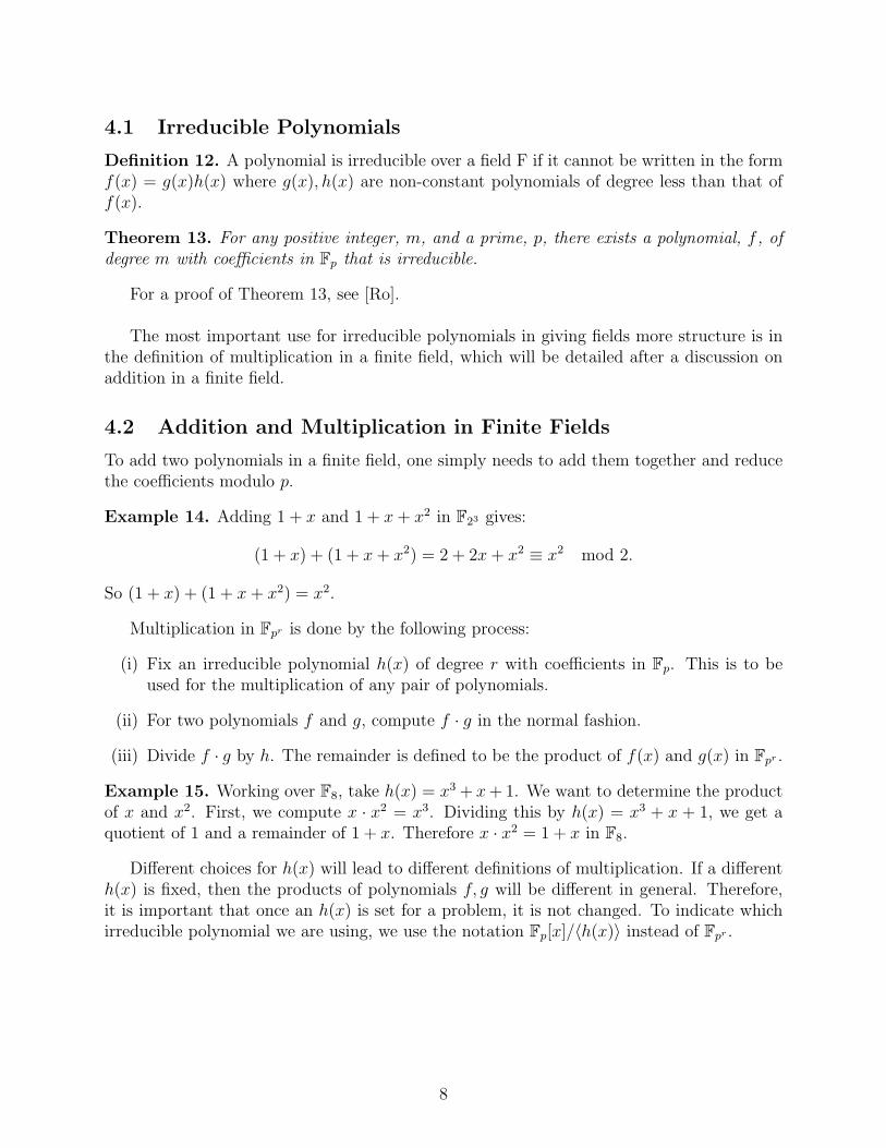
Example 15. Working over F8, take h(x) = x3 + x + 1. We want to determine the productof x and x2. First, we compute x · x2 = x3. Dividing this by h(x) = x3 + x + 1, we get aquotient of 1 and a remainder of 1 + x. Therefore x · x2 = 1 + x in F8.
Different choices for h(x) will lead to different definitions of multiplication. If a differenth(x) is fixed, then the products of polynomials f, g will be different in general. Therefore,it is important that once an h(x) is set for a problem, it is not changed. To indicate whichirreducible polynomial we are using, we use the notation Fp[x]/〈h(x)〉 instead of Fpr .
8
4.3 Constructing Finite Fields Using Primitive Polynomials
We now have enough knowledge of finite fields and polynomials to examine an alternativemethod of constructing finite fields. In fact, one can use certain irreducible polynomials towrite the elements of a the field as powers of a single element. This is key in describing thealgebraic interleavers used in turbo codes, where field arithmetic is done.
For clarification, a brief side note must be made before moving on. Typically, the variableα is used instead of x when constructing finite fields:
F8 = {0, 1, α, α2, 1 + α, 1 + α2, α + α2, 1 + α + α2}.
The following definition describes the type of polynomial used to write write the nonzeroelements of a field as powers of a single variable α.
Definition 16. We say that an irreducible polynomial h(x) ∈ Fp[x] of degree r is calledprimitive if Fp[x]/〈h(x)〉 = {0, 1, α, α2, . . . , αpr−2}.
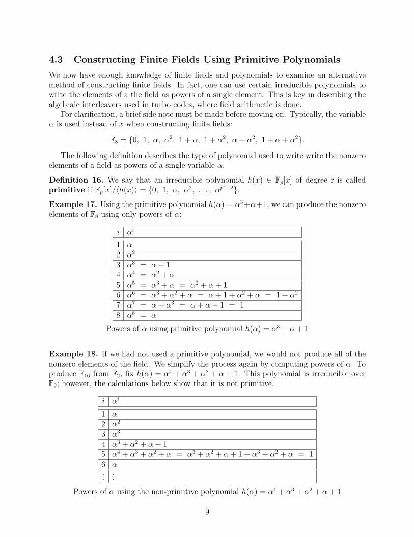
Example 17. Using the primitive polynomial h(α) = α3+α+1, we can produce the nonzeroelements of F8 using only powers of α:
i αi
1 α2 α2
3 α3 = α + 14 α4 = α2 + α5 α5 = α3 + α = α2 + α + 16 α6 = α3 + α2 + α = α + 1 + α2 + α = 1 + α2
7 α7 = α + α3 = α + α + 1 = 18 α8 = α
Powers of α using primitive polynomial h(α) = α3 + α + 1
Example 18. If we had not used a primitive polynomial, we would not produce all of thenonzero elements of the field. We simplify the process again by computing powers of α. Toproduce F16 from F2, fix h(α) = α4 + α3 + α2 + α + 1. This polynomial is irreducible overF2; however, the calculations below show that it is not primitive.
i αi
1 α2 α2
3 α3
4 α3 + α2 + α + 15 α4 + α3 + α2 + α = α3 + α2 + α + 1 + α3 + α2 + α = 16 α...
...
Powers of α using the non-primitive polynomial h(α) = α4 + α3 + α2 + α + 1
9

The following theorem promises the existence of primitive polynomials for use in theconstruction of a finite field.
Theorem 19. For any positive integer r, there exists a primitive polynomial of degree r overFp.
For a proof of theorem 19, see [Pr].
5 Monomial Orders
Another way in which interleavers can be varied is through monomial orderings. We willuse monomial orders as a way to order vectors before the components are permuted. Theseorders are discussed in further detail in Section 6. To begin, we will first look at the definitionof total orders.
Definition 20. We say “<” is a total order on Zn if and only if all the following hold:
(i) for all α 6= β ∈ Zn, α < β or β < α
(ii) for all α ∈ Zn, α ≮ α
(iii) for all α, β, γ ∈ Zn, if α < β and β < γ, then α < γ
The next definition places the final two conditions on an order for it to be called amonomial order, which can then be used in the construction of an interleaver.
Definition 21. A total order on Zn is called a monomial order if and only if
(A) for all α ∈ Nn, if α 6= 0, then α > 0
(B) for all α, β, γ ∈ Zn, if α > β, then α + γ > β + γ
5.1 Types of Monomial Orderings
There are three types of orderings that we will consider; lexicographic, graded lexicographic,and graded reverse lexicographic. Their definitions all follow.
Definition 22. Lexicographic Order is the order such that α < β if and only if the firstnon-zero component of β − α is positive.
Example 23. Let α = (0, 1, 3,−2, 6) and β = (0, 1, 3, 10,−20). After computing β − α =(0, 0, 0, 12,−26), we can see that the first nonzero component, 12, is positive. Therefore,α < β.
Definition 24. Graded Lexicographic Order is the order such that α < β if and only if∑ni=1 αi <
∑ni=1 βi or
∑ni=1 αi =
∑ni=1 βi and the leftmost nonzero component of β − α
is positive, where αi and βi represent the ith components of α and β respectively.
10

Example 25. Let α = (0, 1, 3,−2, 6) and β = (0, 1, 3, 10,−6). Now,∑n
i=1 αi =∑n
i=1 βi =8. Therefore, we need to look at β−α = (0, 0, 0, 12,−12). The leftmost nonzero component,12, is positive. Hence, α < β.
Definition 26. Graded Reverse Lexicographic Order is the order such that α < βif and only if
∑ni=1 αi <
∑ni=1 βi or
∑ni=1 αi =
∑ni=1 βi and the rightmost nonzero
component of β − α is negative, where αi and βi represent the ith component of α and βrespectively.
Example 27. Let α = (0, 1, 3,−2, 6) and β = (0, 1, 3, 10,−6). Now,∑n
i=1 αi =∑n
i=1 βi =8. Consequently, we need to look at β − α = (0, 0, 0, 12,−12). The rightmost nonzerocomponent, -12, is negative so α < β.
We now note a theorem regarding monomial orderings that was crucial in the programwe used to create turbo code interleavers. The interleaver creation program that we createduses an ordering matrix as one of its arguments.
Theorem 28. Let M be an n by n invertible matrix with nonnegative, real entries. Forα, β ∈ Nn, define α < β if and only if the leftmost nonzero component of M(β − α) ispositive. Then, this order is a monomial order.
For a proof of Theorem 28, see [JoMo]. From Theorem 28, one can see that thereare infinitely many monomial orderings, since the entries of a matrix can be created frominfinitely many numbers.
6 Constructing Algebraic Interleavers with Finite Fields
In this section, we will construct interleavers using the tools of the previous sections. Ourpermutation will consist of a composition of maps:
Zprπ1−→ (Zp)
r π2−→ Fprπ3−→ Fpr
π−12−→ (Zp)
r π−11−→ Zpr .
The following steps detail the procedure for constructing an algebraic interleaver:
(i)A Using base p representation: Rewrite each integer c in Zpr in its base p representation:c = c0 + c1p
1 + c2p2 + ... + cr−1p
r−1. Then place the coefficients of c into a vector:π1(c) = (c0, c1, ..., cr−1).
(i)B Using a monomial ordering: For a given monomial ordering, order the vectors of (Zp)r
in ascending order: w0 < ... < wpr−1. Then define π1(c) = wc.
(i) Define π2(w0, w1, ..., wr−1) =∑r−1
i=0 wiαi.
(ii) Choose π3 : Fpr → Fpr to be any permutation of Fpr . For our studies, π3 is usually ofthe form x 7→ xi for some i.
11

Example 29. Here is an example using the lexicographic order and the permutation x 7→ x3:
F8 → F8 by x 7→ x3
F8 = F2/〈x3 + x + 1〉
Z23 (Z2)3 F23 F23 (Z2)
3 Z23
0 (0, 0, 0) 0 0 (0, 0, 0) 01 (0, 0, 1) α2 1 + α2 (1, 0, 1) 52 (0, 1, 0) α 1 + α (1, 1, 0) 63 (0, 1, 1) α + α2 1 + α + α2 (1, 1, 1) 74 (1, 0, 0) 1 1 (1, 0, 0) 45 (1, 0, 1) 1 + α2 α + α2 (0, 1, 1) 36 (1, 1, 0) 1 + α α2 (0, 0, 1) 17 (1, 1, 1) 1 + α + α2 α (0, 1, 0) 2
6.1 Monomial Permutations
In our research, we tested only monomial permutations rather than polynomial permutations.We originally tried to create permutation polynomials, however these took both a long timeto calculate and run in simulations. Because monomial permutations were quicker to generateand test, they were the most practical for us to use.
Definition 30. A permutation monomial is a monomial that is also a permutation inZp → Zp where p is prime.
The following theorems give the criteria for permutation monomials for Zp → Zp whenp is prime. These provided us with an easier way of generating permutations to use, alongwith an assuredness that they were indeed permutations.
Theorem 31. If p is prime and i is an integer relatively prime to p − 1, then fi : Zp →Zp given by fi(x) = xi is a permutation.
Proof. Suppose that p is prime and i is an integer relatively prime to p. Since i is relativelyprime to p, the gcd(i, p−1) = 1. This implies that there exist a, b ∈ Z such that ai+b(p−1) =1. Then x(ai+b(p−1)) = x1. Also, gcd(x, p) = 1 when x ∈ {1, ..., p − 1}. By Fermat’s LittleTheorem, xp−1 ≡ 1 mod p. Then,
x = x1
= x(ai+b(p−1))
= xaixb(p−1)
= xai1b
= xai.
12

When x = 0, we have fi(0) = 0. As we are working in a finite field, fi is invertible if wecan find j such that xij = x. Furthermore, if fi is invertible, then this implies that it is apermutation. We know fi is invertible because xai = x. So, it is a permutation.
In fact, a more general result holds, which is given in the following theorem.
Theorem 32. The monomial xi ∈ Fq[x] is a permutation monomial of Fq if and only ifgcd(i, q − 1) = 1.
For a proof of Theorem 32 see [JoMo].
7 Dispersion
In order to study the “randomness” of an interleaver, we must calculate the dispersion.This property will help us compare the distance between two values in Zq and the distancebetween their permuted images. A high dispersion indicates a variety of the permuteddistances between the elements. The first step of calculating the dispersion is acquiring acomplete list of differences.
Definition 33. Given a permutation π of Zq, the list of differences of π is defined to bethe set
D(π) = {(j − i, π(j)− π(i)) | 0 ≤ i < j < q}.
Example 34. We compute the list of differences for the following permutation:
π =
(0 1 2 3 4 54 2 5 0 3 1
).
We begin by calculating all of the pairs for which the input values are of distance 1 awayfrom each other:
(1− 0, π(1)− π(0)) = (1,−2),
(2− 1, π(2)− π(1)) = (1, 3),
(3− 2, π(3)− π(2)) = (1,−5),
(4− 3, π(4)− π(3)) = (1, 3),
and(5− 4, π(5)− π(4)) = (1,−2).
So, the first elements of the set D(π) are (1,−2), (1, 3), and (1,−5). Because the list ofdifferences is a set, the repeated elements are not to be counted twice. We can continuecalculating the remaining pairs by checking inputs that are 2, 3, 4, and 5 away from eachother. Hence, the permutation has the following list of differences:
D(π) = {(1,−2), (1, 3), (1,−5), (2, 1), (2,−2), (3,−4), (3, 1), (4,−1), (5,−3)}.
Therefore,|D(π)| = 9.
13

Definition 35. Given a permutation π, the dispersion of π is given by
|D(π)|(q2
) =|D(π)|q(q−1)
2
From the previous example, we see that q = 6 because the permutation acts on 6 objects.Furthermore, we know that the cardinality of D(π) is 9. We can now calculate the dispersionusing the definition:
|D(π)|q(q−1)
2
=9
6(5)2
=9302
=3
5.
7.1 Conjecture
Pursuant to a question asked during a presentation, we decided to investigate whether ornot we could determine what proportion of permutations of a given size have a dispersionaround 0.8. This proved to be of particular interest, as permutations with this dispersiontend to have the lowest bit error rates.
Upon looking into this, we have discovered that the mean dispersion for all permutationsof a given size are around .81. As one increases the size of the set acted on, the averagedispersion appears to converge to a number between 0.813 and .814. The standard deviationaway from this mean also decreases, and appears to go to zero, as the permutation lengthgets larger.
We obtained the following data by testing samples of permutations of different lengthsand calculating the average dispersion based on these samples. We also calculated thestandard deviation away from this mean. The first chart has been calculated exactly, bytesting all possible permutations of the given permutation sizes. The data in the secondand third charts was obtained using sample data for the given block lengths. For sizes of 10through 90, we used a sample size of 100000 permutations selected randomly of all possiblepermutations, and for lengths of 100 to 1000, we used random sample sizes of 10000 fromall possible permutations. The reason for this is that as the permutation size increases, thetime to calculate the data also increases.
Exact Average Dispersion for Permutation Sizes Between 2 and 10Length Average Dispersion Standard Deviation
2 1 03 0.8889 0.17214 0.8472 0.17665 0.8467 0.14956 0.8383 0.12747 0.8355 0.10008 0.8319 0.08669 0.8301 0.073710 0.8280 0.0657
14
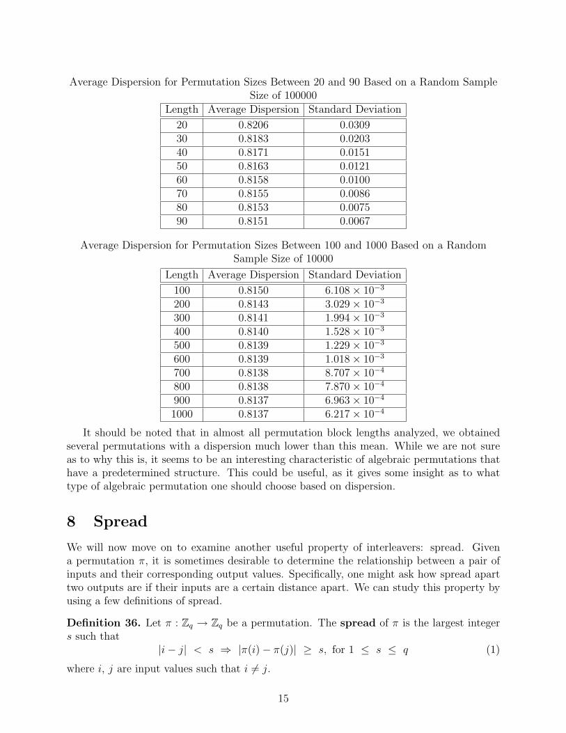
Average Dispersion for Permutation Sizes Between 20 and 90 Based on a Random SampleSize of 100000
Length Average Dispersion Standard Deviation
20 0.8206 0.030930 0.8183 0.020340 0.8171 0.015150 0.8163 0.012160 0.8158 0.010070 0.8155 0.008680 0.8153 0.007590 0.8151 0.0067
Average Dispersion for Permutation Sizes Between 100 and 1000 Based on a RandomSample Size of 10000
Length Average Dispersion Standard Deviation
100 0.8150 6.108× 10⁻³
200 0.8143 3.029× 10⁻³
300 0.8141 1.994× 10⁻³
400 0.8140 1.528× 10⁻³
500 0.8139 1.229× 10⁻³
600 0.8139 1.018× 10⁻³
700 0.8138 8.707× 10⁻⁴
800 0.8138 7.870× 10⁻⁴
900 0.8137 6.963× 10⁻⁴
1000 0.8137 6.217× 10⁻⁴
It should be noted that in almost all permutation block lengths analyzed, we obtainedseveral permutations with a dispersion much lower than this mean. While we are not sureas to why this is, it seems to be an interesting characteristic of algebraic permutations thathave a predetermined structure. This could be useful, as it gives some insight as to whattype of algebraic permutation one should choose based on dispersion.
8 Spread
We will now move on to examine another useful property of interleavers: spread. Givena permutation π, it is sometimes desirable to determine the relationship between a pair ofinputs and their corresponding output values. Specifically, one might ask how spread aparttwo outputs are if their inputs are a certain distance apart. We can study this property byusing a few definitions of spread.
Definition 36. Let π : Zq → Zq be a permutation. The spread of π is the largest integers such that
|i− j| < s ⇒ |π(i)− π(j)| ≥ s, for 1 ≤ s ≤ q (1)
where i, j are input values such that i 6= j.
15

Proposition 37. The spread of a permutation is always greater than or equal to 1.
Proof. For s = 1, we must test all input values that have a distance of less than 1 betweenthem. Since i 6= j, there will never exist two input values that have a distance of 0 betweenthem. Thus, the antecedent of (1) is always false. Consequently, the statement is alwaystrue for s = 1. Hence, the spread of any permutation must be greater than or equal to 1.
Proposition 38. If s ≥ 2 and satisfies |i− j| < s ⇒ |π(i)− π(j)| ≥ s for all i 6= j, then forall s′ ≤ s,
|i− j| < s′ ⇒ |π(i)− π(j)| ≥ s′
for all i 6= j.
Proof. Let s ≥ 2 and suppose |i− j| < s ⇒ |π(i)− π(j)| ≥ s for all i 6= j. Suppose for somes′ ≤ s, |i − j| < s′. Since |i − j| < s′ ≤ s, |π(i) − π(j)| ≥ s ≥ s′. Therefore, for all s′ ≤ s,|i− j| < s′ ⇒ |π(i)− π(j)| ≥ s′ for all i 6= j.
Example 39. For the following permutation, we calculate spread:
π =
(0 1 2 3 4 54 2 5 0 3 1
).
We look at all the pairs for which |i− j| < 2, and check to see if |π(i)− π(j)| ≥ 2.Thus,
|π(1)− π(0)| = |2− 4| = 2,
|π(2)− π(1)| = |5− 1| = 4,
|π(3)− π(2)| = |0− 5| = 5,
|π(4)− π(3)| = |3− 0| = 3,
and|π(5)− π(4)| = |1− 3| = 2.
As we can see, all pairs of inputs that are less than 2 away from each other have a permuteddistance of at least 2 away from each other. Hence, s = 2 is a possible spread. We mustnow consider the case for which s = 3. We examine all the pairs for which |i − j| < 3and check if |π(i)−π(j)| ≥ 3. First we will consider input values that are of distance 2 awayfrom each other; if the definition holds for these inputs, we will check input values that areof distance 1 away from each other. Thus
|π(2)− π(0)| = |4− 5| = 1,
|π(3)− π(1)| = |2− 0| = 2,
|π(4)− π(2)| = |5− 3| = 2,
and|π(5)− π(3)| = |0− 1| = 1.
16
We can see that the input values 2 and 0 produce output values that are only of distance1 away from each other, and so the spread cannot possibly be 3. Therefore, by Proposition38, the spread of π is 2. s = 2.
8.1 The Upper Bound for Spread
We will now present several lemmas and theorems with respect to the upper bound for spread.Theorem 43 gives an upper bound for spread that we originally found in our research; thefollowing example and lemmas prepare for the theorem.
Consider the statement:
|i− j| < s ⇒ |π(i)− π(j)| ≥ s,
and thus define
A = {(i, j) ∈ Zq × Zq| i 6= j, 1 ≤ i, j ≤ q},Bs = {(i, j) ∈ Zq × Zq | i 6= j and |i− j| < s}, and
Cs = {(i, j) ∈ Zq × Zq | i 6= j and |π(i)− π(j)| ≥ s}.
Then |A| = q2 − q, since there are q2 − q possible pairs (i, j) where i 6= j. We now turn toa brief example that will help us determine a formula for Bs.
Example 40. For Z5 × Z5, we can list the pairs (i,j).
A list of all pairs (i, j), where 1 ≤ i, j ≤ q:
(0, 0) (1,0) (2,0) (3, 0) (4, 0)
(0,1) (1, 1) (2,1) (3,1) (4, 1)
(0,2) (1,2) (2, 2) (3,2) (4,2)
(0, 3) (1,3) (2,3) (3, 3) (4,3)
(0, 4) (1, 4) (2,4) (3,4) (4, 4)
The bolded sets make up B2 = {(i, j) ∈ Z5 × Z5 | i 6= j and |i − j| < 2}, since they arecomposed of inputs less than 2 apart. There are 4+4 = 8 sets that are bolded. Thus |B2| =2(4) = 2(5− 1). In the above chart, another chart for s = 3 is included, which combines thebolded diagonals with the italicized diagonals. Therefore, there are 8+3+3 = 8+6 = 14 setsthat hold true. Thus |B3| = 2(4) + 2(3) = 2(5− 1) + 2(5− 2). Similarly, for s = 4, there are14+2+2 = 16 sets that hold true, so |B4| = 2(4)+2(3)+2(2) = 2(5−1)+2(5−2)+2(5−3).We write the preceding formulas vertically to see the pattern emerging:
s = 2 : |B2| = 2(q − 1)
s = 3 : |B3| = 2(q − 1) + 2(q − 2)
s = 4 : |B4| = 2(q − 1) + 2(q − 2) + 2(q − 3)...
17

The following lemma results from generalizing the specific values for |Bs| in the precedingexample.
Lemma 41. For any q and s, we find |Bs| = 2∑s−1
k=1(q − k) = −2q + s + 2qs− s2.
Now that we have computed |Bs|, we turn find the cardinality of Cs.
Lemma 42. For any q and s, we find |Cs| = q2 + q − s− 2qs + s2.
Proof. Let π be a permutation. We can write Cs as:
Cs = {(i, j) ∈ Zq × Zq | i 6= j and |π(i)− π(j)| ≥ s}= {(π−1(i), π−1(j)) ∈ Zq × Zq | i 6= j and |i− j| ≥ s}= {(i, j) ∈ Zq × Zq | i 6= j and |i− j| ≥ s}
It is now clear that, for all s, A = Bs ∪Cs. Then |A| = |Bs ∪Cs| = |Bs|+ |Cs|. Substitutingin the respective values and solving for |Cs|, we have
q2 − q = 2s−1∑j=1
(q − j) + |Cs|,
and so
|Cs| = q2 − q − 2s−1∑j=1
(q − j)
= q2 + q − s− 2qs + s2.
Theorem 43. [AMSSI 2006] An upper bound for spread is b12(1 + 2q −
√2q2 − 2q + 1c,
where q is the length of the permutation.
Proof. Let q : Zq → Zq be a permutation with spread s.We consider the inequality |Bs| ≤ |Cs|, using the values for |Bs| and |Cs| as developed in
Lemmas 41 and 42. Since |Bs| ≤ |Cs|, we have
−2q + s + 2qs− s2 ≤ q2 + q − s− 2qs + s2.
Thus,0 ≤ q2 + 3q − 2s− 4qs + 2s2
= 2s2 + (−2− 4q)s + (q2 + 3q).
We solve the corresponding equality for s, using the quadratic equation:
s =(2 + 4q)±
√(2 + 4q)2 − 4 · 2 · (q2 + 3q)
2 · 2.
18
Simplifying, we have
s =1
2
((1 + 2q)±
√2q2 − 2q + 1
).
Since 12
((1 + 2q) +
√2q2 − 2q + 1
)≥ 1
2
((1 + 2q)−
√2q2 − 2q + 1
), by Proposition 38, we
need only consider s = 12
((1 + 2q)−
√2q2 − 2q + 1
).
Reintroducing the inequality leads to s ≤ 12
((1 + 2q)−
√2q2 − 2q + 1
). Since the right
hand side may not be an integer, we take the floor of this function to find our upper boundfor spread is ⌊
1
2
((1 + 2q)−
√2q2 − 2q + 1
)⌋.
It can also be shown that a more refined upper bound for the spread of a permutation ofZq is b√qc. The lemma below shows that there exists a permutation of Zq with spread
√q
whenever q is a perfect square.
Lemma 44. [AMSSI 2006] If q = s2, then there exists a permutation with spread s.
Proof. Let i, j ∈ Zq such that |i − j| < s. Without loss of generality, i > j. For all inputvalues i 6= j, we can write i and j in base s; i.e., i = a0 + sa1, and j = b0 + sb1, where0 ≤ an, bn ≤ s − 1. We define π : Zq → Zq by π(a0 + sa1) = (s − 1 − a1) + sa0 andπ(b0 + sb1) = (s− 1− b1) + sb0.
Since |i − j| < s and i > j, either a1 = b1 or a1 = b1 + 1. We consider the two casesseparately.
Case 1: a1 = b1. Now,
|i− j| = |a0 + sa1 − b0 − sa1| = |a0 − b0|,
and by hypothesis, |a0 − b0| < s. Since i 6= j, |a0 − b0| ≥ 1. Thus,
|π(i)− π(j)| = |π(a0 + sa1)− π(b0 + sb1)|,= |(s− 1− a1) + sa0 − (s− 1− a1) + sb0|,= s|(a0 − b0)|,≥ s.
Case 2: a1 = b1 + 1. So
|i− j| = |a0 + s(b1 + 1)− b0 − sb1| = |a0 − b0 + s|
and by hypothesis, |a0 − b0 + s| < s. Thus (a0 − b0) < 0, so a0 < b0, and by definition0 < |a0 − b0| ≤ s. When comparing the respective images of i and j,
|π(i)− π(j)| = |(s− 1− b1 − 1) + sa0 − (s− 1− b1)− sb0)|= | − 1 + s(a0 − b0)|
19

and since both −1 and s(a0 − b0) are negative,
| − [1 + s(b0 − a0)]| = 1 + s(b0 − a0) ≥ s
Using the ideas of Lemma 44, we can prove a more general result, namely, that for anypositive integer q, there exists a permutation with spread b√qc. We begin with an examplethat helps motivate the ideas in the proof.
Example 45. We can design permutations that achieve the maximum spread for a givenpermutation length q. In this example, we take q = 9. Then we define each Ri for 0 ≤ i ≤ 2as follows:
R2 = (2, 5, 8)
R1 = (1, 4, 7)
R0 = (0, 3, 6)
and so R = (2, 5, 8, 1, 4, 7, 0, 3, 6), in which case
π =
(0 1 2 3 4 5 6 7 82 5 8 1 4 7 0 3 6
)By constructing π in this manner, we create a permutation. In this example, π has a
spread of 3 =√
9.
Lemma 46. [AMSSI 2006] If q ≥ s2, then there exists a permutation, π, with spread atleast s.
Proof. Generalizing the notions developed in Example 45, for each integer i such that 0 ≤ i ≤s−1, define Ri to be the finite sequence of elements of Zq given by Ri = i, i+s, i+2s, ..., i+mis,where mi is the largest integer such that i + mis ≤ q− 1. Then, define R to be the sequencethat is the concatenation of the sequences Rs−1, Rs−2, ..., R2, R1, R0. Define π : Zq ⇒ Zq tobe the permutation that sends 0, 1, 2, ..., q − 1 to the terms of R, respectively.
The terms on the ends of each row Ri are the largest in their row, with the maximum ofthese being q − 1 (since all elements are in the range 0, ..., q − 1) and smallest being q − s,because there are s rows. Thus, i + mis ≥ q − s. Since 1 ≤ i ≤ s − 1 and, by hypothesis,q ≥ s2, we have
(s− 1) + mis ≥ i + mis
≥ q − s
≥ s2 − s,
and somis ≥ s2 − 2s + 1.
Thus,
mi ≥ s− 2 + 1s. (2)
20

We now proceed to show that the spread of π is s. Let k, l ∈ Zq such that k 6= l and|k − l| < s. Without loss of generality, suppose l < k. Since |k − l| < s and each row Ri
has at least s terms, either π(k) and π(l) are in the same row or they are in adjacent rowsRi, Ri−1. We consider these two cases separately.
If π(k), π(l) ∈ Ri for some index i, then for some δ, γ such that δ > γ, π(k) = i + δs andπ(l) = i + γs. Then |π(k)− π(l)| = (δ − γ)s > s.
Otherwise, if π(k) is a term of Ri and π(l) is a term of Ri−1 (where 1 ≤ i ≤ s− 1), thenfor some δ, γ, π(k) = i + δs and π(l) = (i− 1) + γs. The last term of Ri is i + mis and so
π−1(i + mis)− k = π−1(i + mis)− π−1(i + δs) = mi − δ. (3)
Moreover, since i− 1 is the first term of Ri−1, and i + mis is the last term of Ri,
π−1(i− 1)− π−1(i + mis) = 1. (4)
Since π(l) = (i− 1) + γs is also a term of Ri−1,
l − π−1(i− 1) = π−1((i− 1) + γs)− π−1(i− 1) = γ (5)
Putting (3), (4), and (5) together,
l − k =(l − π−1(i− 1)
)+
(π−1(i− 1)− π−1(i + mis)
)+
(π−1(i + mis)− k
)= γ + 1 + mi − δ.
Since we have l − k < s, γ − δ + mi + 1 < s, and so
γ − δ + mi + 2 ≤ s.
Thus,
γ − δ ≤ s− 2−mi (6)
Putting (2) and (6) together, we have
γ − δ ≤ s− 2−mi
≤ s− 2− s + 2− 1
s
≤ −1
s
Rearranging the last inequality leads to
δ − γ ≥ 1
s. (7)
Then, δ > γ by (7), which implies δ − γ ≥ 1, and so we have
|π(k)− π(l)| = |(i + δs)− ((i− 1) + γs)|= 1 + (δ − γ)s
≥ s.
21

It has now been shown that, for a given spread s, one can find a sufficiently large fieldsuch that the spread of at least one permutation of the field is s. This might lead one towonder if spread has an upper bound related to the size of the permutation. The followingtheorem shows that a bound exists.
Theorem 47. [AMSSI 2006] For any permutation π of Zq, the spread of π ≤ b√qc. Infact, by Lemma 46, there exists a permutation with spread equal to b√qc.
Proof. Let π be a permutation of Zq with spread s. Consider and interval I = {k, k+1, ..., k+(s − 1)} ⊆ Zq such that s − 1 ∈ I, and define π(I) = {π(j)|j ∈ I}. Because the spread ofπ is s, and since all the elements of I are within a distance of s− 1 of each other, all of theimages in π(I) must be a distance of at least s from one another. Therefore, 0, 1, ..., s − 2are not in π(I). Write the s elements of I in ascending order, i.e., π(I) = {α1, α2, ..., αs}where α1 < α2 < ... < αs. Since 0, 1, ..., s− 2 are not in π(I), s− 1 is the smallest entry ofπ(I). Therefore, α1 = s− 1. Since the elements of π(I) are at least s apart from each other,αj − αj−1 ≥ s for all j = 2, 3, ..., s. Thus
αs − α1 = (αs − αs−1) + (αs−1 + αs−2) + · · ·+ (α2 − α1)
≥ (s− 1)s
= s2 − s.
Rearranging, we obtain
αs ≥ α1 + s2 − s
= s− 1 + s2 − s
= s2 − 1.
Therefore, since αs ∈ Zq, we have q−1 ≥ αs, and so q−1 ≥ s2−1. Thus, q ≥ s2, so√
q ≥ s.Since s is an integer, it follows that
s ≤ b√qc.
8.2 Other Measures of Spread
We will now consider some other measures of spread in order to study the distance betweenpermuted values. There are four measures that can be examined: spreading factors, extremespreading factors, s-parameters, and spread factors.
Definition 48. The spreading factors of π = Zq → Zq are all points (s, t) that satisfy
|i− j| < s ⇒ |π(i)− π(j)| ≥ t, (8)
for all i, j ∈ Zq such that i 6= j.
Calculating the spreading factors is an extremely long process without a computer pro-gram, as the following example shows.
22

Example 49.
π =
(0 1 2 3 4 5 6 7 8 9 100 3 6 9 1 4 7 10 2 5 8
)We consider (2, 3) and determine if it is a spreading factor. That is, we test all pairs of inputvalues (i, j) such that |i− j| < 2 and determine if the distance between their output values|π(i)− π(j)| is at least 3. Starting with input values (2, 1), we see that,
|2− 1| < 2 and |π(2)− π(1)| = |6− 3| = 3 ≥ 2
The same process has to be repeated for input values (3, 2), (4, 3), ..., (10, 9) because they arepairs of indices of distance less than 2 away from each other. If (8) is satisfied for all thesepairs in addition to (2, 1), then we know that (2, 3) is a spreading factor. In order to get allpossible spreading factors, this process must be completed for all pairs (s, t) where s, t ∈ Zq.After checking all possible spreading factors, we can complete a graph of all the spreadingfactors that were found. The following graph is a plot of all the spreading factors of π; eachone is marked with an x.
Figure 5: Plot of Spreading Factors, Extreme Spreading Factors, and the s-Parameter
23

We can study this graph further and gain more insight into spread if we introduce thefollowing properties: extreme spreading factors and s-parameters.
Definition 50. A spreading factor (s, t) is an extreme spreading factor if either (s+1, t)or (s, t + 1) is not a spreading factor.
Example 51. The spreading factors with boxes around them in Figure 5 are extreme spread-ing factors because spreading factors either do not exist directly to the right or directly abovethem.
Definition 52. The s-parameter is the maximum value of s such that for some s ≤ t,(s, t) is an extreme spreading factor.
Example 53. In order to find the s-parameter in Figure 5, we consider all the extremespreading factors. The largest value of s such that s ≤ t is s = 3. Therefore, the s-parameteris 3 and is circled in Figure 5.
Definition 54. For all input values i < j and output values π(i), π(j), and q representingthe length of the permutation, let
δ(i, j) = |i− j|q + |π(i)− π(j)|qwhere
|x− y|q = min[(x− y) mod q, (y − x) mod q]
Another measure of spread we examined was the spread factor, not to be confused withspreading factors. The spread factor is not equal to spread, however, it seems that when oneincreases, they both increase, due to the definitions of both.
Definition 55. The spread factor of a permutation π is the minimum δ(i, j) over all i < j.
Example 56. Consider the following permutation:
π =
(0 1 2 3 4 54 2 5 0 3 1
)In order to find the spread factor, we must first make a list of all the pairs of input valuesfor which i < j.
(0, 1) (0, 2) (0, 3) (0, 4) (0, 5)(1, 2) (1, 3) (1, 4) (1, 5)(2, 3) (2, 4) (2, 5)(3, 4) (3, 5)(4, 5)
Now that we have all possible pairs, we can now calculate δ(i, j) for each pair.
δ(0, 1) = |0− 1|6 + |π(0)− π(1)|6 = 3 δ(0, 2) = |0− 2|6 + |π(0)− π(2)|6 = 3δ(0, 3) = |0− 3|6 + |π(0)− π(3)|6 = 5 δ(0, 4) = |0− 4|6 + |π(0)− π(4)|6 = 3δ(0, 5) = |0− 5|6 + |π(0)− π(5)|6 = 4 δ(1, 2) = |1− 2|6 + |π(1)− π(2)|6 = 4δ(1, 3) = |1− 3|6 + |π(1)− π(3)|6 = 4 δ(1, 4) = |1− 4|6 + |π(1)− π(4)|6 = 4δ(1, 5) = |1− 5|6 + |π(1)− π(5)|6 = 3 δ(2, 3) = |2− 3|6 + |π(2)− π(3)|6 = 2δ(2, 4) = |2− 4|6 + |π(2)− π(4)|6 = 4 δ(2, 5) = |2− 5|6 + |π(2)− π(5)|6 = 5δ(3, 4) = |3− 4|6 + |π(3)− π(4)|6 = 4 δ(3, 5) = |3− 5|6 + |π(3)− π(5)|6 = 3δ(4, 5) = |4− 5|6 + |π(4)− π(5)|6 = 3
24

We can see that the pair with the minimum value of δ(i, j) is (2, 3), with a value of 2. Hence,the spread factor is 2 for this permutation.
8.3 Spread and S-Parameters Coincide: Our Theoretical Results
It can be shown that the s-parameter of a permutation is equal to its spread. Before westate this theorem and its proof, we will first prove three lemmas. The first lemma dealswith a bound for the spreading factor.
Lemma 57. [AMSSI 2006] The sth column of the spreading factor plot is bounded fors ≥ 2; that is for all s ≥ 2, there are only finitely many values of t such that (s, t) is aspreading factor.
Proof. For any permutation of Zq, the largest distance any two i, j ∈ Zq can be from oneanother is q − 1. This is also true for any two π(i), π(j). By the definition of spreadingfactor, |i− j| < s ⇒ |π(i)− π(j)| ≥ t. The value of t can be at most q − 1. Thus, there arefinitely many values of t such that (s, t) is a spreading factor.
The following lemma guarantees the existence of an extreme spreading factor based onthe existence of a spreading factor (s, s).
Lemma 58. [AMSSI 2006] If (s, s) is a spreading factor, then there exists s ≤ t suchthat (s, t) is an extreme spreading factor.
Proof. Let (s, s) be a spreading factor. By Lemma 57, let t be the upper bound for the sth
column. Then, (s, t + 1) is not a spreading factor. Therefore (s, t) is an extreme spreadingfactor.
The final lemma guarantees that (s, s) is a spreading factor if s is the s-parameter.
Lemma 59. [AMSSI 2006] If s is the s-parameter of a permutation, then (s, s) is aspreading factor.
Proof. For some t ≥ s, let (s, t) be an extreme spreading factor as defined in Definition 52.Then by the definition of the s-parameter, we have for all i 6= j, |i−j| < s ⇒ |π(i)−π(j)| ≥ t.Thus for all t′ < t, all pairs (s, t′) are spreading factors, including t′ = s. Thus (s, s) is aspreading factor.
In combining the three lemmas, it is possible to prove a very interesting result, namelythat the definitions of s-parameter and spread are equivalent. Thus, the following theoremlinks the two definitions of spread.
Theorem 60. [AMSSI 2006] The s-parameter of a permutation is equal to its spread.
Proof. Let s be the s-parameter of a permutation. By Lemma 59, (s, s) is a spreading factor.For contradiction, suppose (s + 1, s + 1) is also a spreading factor. By Lemma 58, (s + 1, t)is an extreme spreading factor for some t ≥ s + 1. Since (s + 1, t) is an extreme spreading
25

factor, then the s-parameter is at least s + 1. However, the s-parameter is s, which impliesthat s + 1 ≤ s. This is a contradiction. Therefore, (s + 1, s + 1) is not a spreading factor.
Since (s, s) is a spreading factor, by the definition of spreading factor, |i − j| < s ⇒|π(i) − π(j)| ≥ s. So s satisfies (1). However, since (s + 1, s + 1) is not a spreading factor,then for some i 6= j, |i − j| < s + 1 ; |π(i) − π(j)| ≥ s + 1. So s + 1 does not satisfy (1).Therefore, s is the spread. Thus, the s-parameter of a permutation is equal to its spread.
9 Simulations
In order to test the effectiveness of our interleavers, we ran various simulations in a turbosimulator program. The turbo simulator was developed by Yufei Wu [Wu]. To run thesimulation, specify a field, a monomial order, and a polynomial. In doing our simulationswe worked with the following items:
Definition 61. Bits are the pieces of information that make up our messages. They are inthe form 0 or 1.
Definition 62. Frames finite blocks of data of a specified length. In our simulations, thislength is the cardinality of the field being used.
Definition 63. The Signal to Noise Ratio (EbN0) is the ratio of the strength of thesignal to the strength of the surrounding noise in decibels (dB). In particular, we will belooking at signal to noise ratios of 0, 0.5, 1, 1.5, and 2 dB.
Definition 64. The Bit Error Rate (BER) is the number of uncorrectable corrupted bitsover the total number of bits sent.
The turbo simulator takes as input five items: a permutation polynomial, a convolutionalcode, a monomial order, the number of decoding iterations, and a frame error limit.
The permutation polynomial and monomial order are those built using the methods fromprevious sections. In our simulator, these were both specified as arguments. The last threeinput items were coded into our turbo simulator during our simulations. The number ofdecoding iterations specified how many times the decoders passed an updated version of themessage back and forth to take advantage of belief propagation. This value was set to 8in our simulations, which means each decoder had 8 chances to try to correct any errorsand check this “corrected” message with the other decoder. The frame error limit was thestopping condition in our simulation. When the number of uncorrectable errors reached thisnumber, the simulation stopped. This number was set at 100 errors in our simulations.
The final BER is calculated after reaching the frame error limit at each signal to noiseratio. By looking at the BER for each signal to noise ratio, we can see how our variousinterleavers performed.
26

10 Results
Our simulations aim to examine how the properties of permutations (spread and dispersion)affect the error-correcting ability of turbo codes and to examine how different monomialorderings may affect a turbo code. We look at these factors over fields of differing sizes.
In general, we have found that in smaller fields, changing interleavers in order to obtaindifferent spreads and dispersions has little effect on the ability of the codes to correct errors.It seems that the fields are too small to allow for much effect of the properties on the turbocodes. However, in larger fields like F28 or F53 , the differences that occur with varyingspreads, dispersions, and monomial orderings can be quite drastic. In practice, much largerfields than even these are used because of improved error correcting ability when using largeblock lengths.
Monomial orderings provide a clear change in permutation action. Without an orderingapplied, the spread of a permutation, using a monomial map, is always one, since 0 and 1 arealways mapped to themselves under any monomial. Thus, monomial orders are a good placeto look to see how dispersion affects a permutation, since by using no monomial ordering onecan keep spread constant. Also, these orders provide insight into how changes in orderingcan affect the performance of a turbo code, even those whose interleavers have similar spreadand dispersion.
Spread and dispersion seem to be distinct factors in turbo code performance. In general,it seems that spread and dispersion have a weak inverse relationship. Thus, for very highspreads, the permutations tend to have relatively small dispersions. Examination of datahas led to the hypothesis that higher dispersion means a better turbo code. Thus, it wouldseem that interleavers with smaller spreads would consequently create a better turbo code,however, we have also seen that spread can give an indication as to turbo code performanceon its own. If dispersion is the same, a higher spread often results in slightly improvedperformance. Thus, though higher dispersion implies better error correcting in most cases,further examination is necessary to find the reasons for any discrepancies and create a soundtheory on turbo code performance. Following are several graphs that illustrate the positivecorrelation between high dispersion and better performance:
27
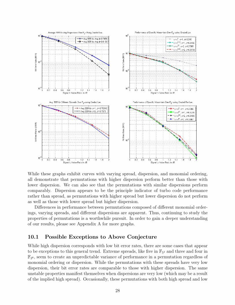
While these graphs exhibit curves with varying spread, dispersion, and monomial ordering,all demonstrate that permutations with higher dispersion perform better than those withlower dispersion. We can also see that the permutations with similar dispersions performcomparably. Dispersion appears to be the principle indicator of turbo code performancerather than spread, as permutations with higher spread but lower dispersion do not performas well as those with lower spread but higher dispersion.
Differences in performance between permutations composed of different monomial order-ings, varying spreads, and different dispersions are apparent. Thus, continuing to study theproperties of permutations is a worthwhile pursuit. In order to gain a deeper understandingof our results, please see Appendix A for more graphs.
10.1 Possible Exceptions to Above Conjecture
While high dispersion corresponds with low bit error rates, there are some cases that appearto be exceptions to this general trend. Extreme spreads, like five in F53 and three and four inF28 , seem to create an unpredictable variance of performance in a permutation regardless ofmonomial ordering or dispersion. While the permutations with these spreads have very lowdispersion, their bit error rates are comparable to those with higher dispersion. The sameunstable properties manifest themselves when dispersions are very low (which may be a resultof the implied high spread). Occasionally, these permutations with both high spread and low
28

dispersion outperform those with higher dispersion. There are only a few examples of theseexceptions, and out of the many block lengths we tested, only two (F28 and F53 specificallyusing lexicographic order) do not seem to follow the generally positive correlation betweenhigh dispersion and low bit error rates. The two examples are:
Here, the curves of permutations with low dispersions perform similarly or better than thosewith high dispersions. Since we found only two exceptions out of the large number of fieldswe tested, further examination of other properties or characteristics of these permutationsis necessary to explain their unexpected behavior.
10.2 A Comparison of Different Monomial Orderings
Different monomial orderings can change the spread, dispersion, and permuted values of apermutation monomial. Thus, it is possible that a particular monomial will perform betterwhen using one monomial ordering over another. For example:
29

Here, x 7→ x32 has the highest dispersion when Graded Reverse Lex is used, as well as thelowest bit error rate. In Lex Ordering, it has the lowest dispersion as well as the highest biterror rate. When comparing Lex and Graded Lex, Graded Lex, with the higher dispersion,has a lower bit error rate. Given the differences in their respective dispersions, however, onemay expect a more noticeable difference in performance. This could possibly be attributedto the small sample sizes we used in the turbo simulator. Still, while the difference is slight,the higher dispersion yields a lower bit error rate.
Similar observations were made when comparing x 7→ x64 in F27 :
Here, the higher dispersion (also in Graded Reverse Lex) once again yields the lowest biterror rate. Note also that the spread is less than the other two, which once again seems toindicate that dispersion is the greater determinant of performance.
When compared to other permutations of the same block length under the same monomialorderings, dispersion seems to be a good indicator of performance. The fact that when thetwo monomial orderings (Lex and Graded Lex) do not perform exactly as expected based ondispersion alone could perhaps indicate that the particular monomial ordering used has someeffect on performance as well. Along these lines, it should be noted that when using GradedReverse Lex in all fields we examined, it is very rare that a permutation has a dispersionless than .7000, with the exception of the mapping x 7→ x, which by default has a very lowdispersion. This is important, as .7000 seems to be a sort of breaking point between goodand poor performance. Permutations with dispersion higher than .7000 perform comparably,while those with dispersion less than .7000 perform with distinctly poorer bit error rates.
10.3 Permutations That Do Not Use Monomial Orders
After examining how permutations performed under different monomial orderings, we lookedat some without any ordering at all. Because we examined only monomials for creating ourpermutations, the spreads for all the permutations created without an imposed ordering isone, simply because 1 and 0 are always mapped next to themselves. With spread beingconstant regardless of the permutation, better comparisons of the effects of dispersion can
30

be made. Here are some comparisons of different average dispersions of permutations inseveral fields. The dispersion values were divided and averaged together in separate intervalsas follows : [0.0000, 0.4999], [0.5000, 0.6999], and [0.7000, 1.0000]. The ranges were basedon how frequently dispersions in certain ranges appear, as well as distinct differences inperformance of different dispersion values/ranges. With the fields we tested, dispersionsnever fell within the second interval. Thus there are only two curves on each graph.
As expected, when different average dispersions are compared, we see that the higherdispersion yields lower bit error rates. Since the value for spread in all permutations is s = 1when no ordering is used, dispersion appears to be the primary indicator for turbo codeperformance; in all examples we tested, high dispersion corresponded to low bit error rates.
10.4 Semi-Random Permutations versus Algebraic Permutations
Definition 65. A semi-random permutation of Zq can be generated by choosing imagesfor 0, 1, ..., q−1, one after the other, so that each stage of the permutation has a pre-specifiedspread. For the full algorithm, see Appendix B.10.1
We compared the performance of semi-random permutations to the performance of thealgebraic permutations we created. We did this in part to see if the method used in construct-ing the permutation had an effect on their performance. When compared with permutations
31
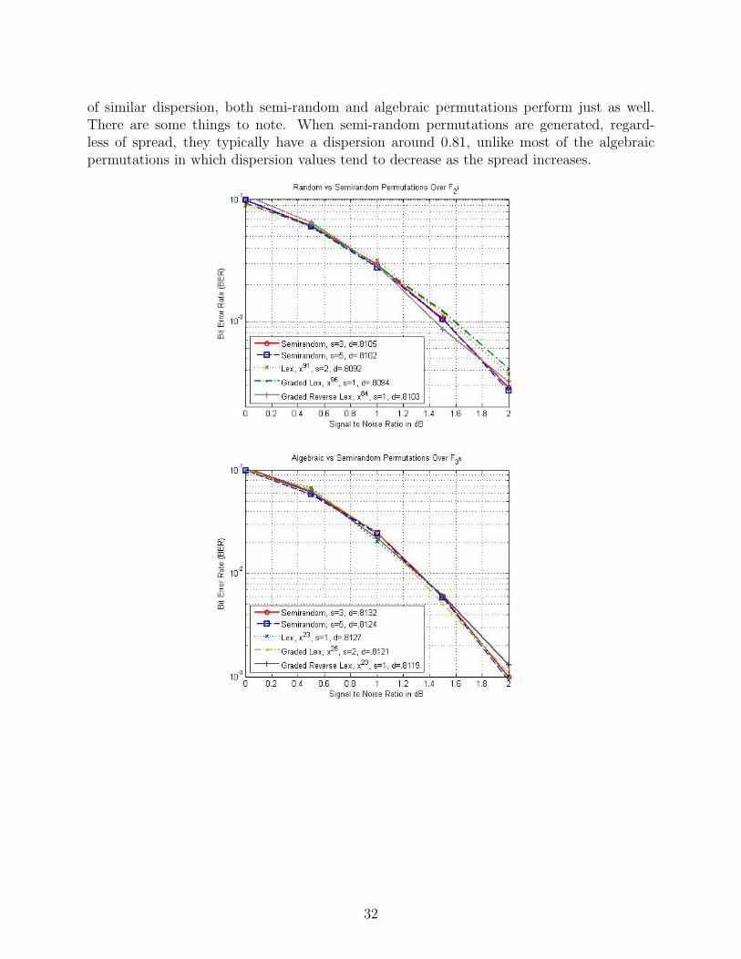
of similar dispersion, both semi-random and algebraic permutations perform just as well.There are some things to note. When semi-random permutations are generated, regard-less of spread, they typically have a dispersion around 0.81, unlike most of the algebraicpermutations in which dispersion values tend to decrease as the spread increases.
32

Thus, because each permutation has a similar dispersion, they all perform in much thesame way. This also demonstrates that the dispersion is a better indicator of performancethan spread.
10.5 Pseudo-Random Permutations versus Algebraic Permutations
Plots of both a pseudo-random permutation and an algebraic one of 212 letters.
The first plot, of the algebraic permutation created using x 7→ x2, has a clear pattern,while the second, of a pseudo-random permutation, lacks any consistent pattern. Becausedispersion is a measure of the randomness of a permutation, we conjecture that the firsthas a low dispersion, while the second has a higher dispersion. In fact, the dispersions ofthe algebraic permutation is 0.2372 and the dispersion of the pseudo-random permutationis 0.8137. Since most of our findings indicate a correspondence between high dispersion andbetter turbo code performance, the second permutation should perform better. Therefore,the goal would be to use an algebraic interleaver that yields a permutation with a higherdispersion, which graphically translates to a plot that lacks a clearly defined pattern. Looking
33
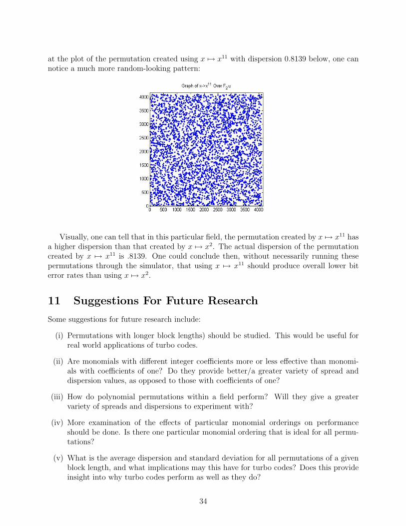
at the plot of the permutation created using x 7→ x11 with dispersion 0.8139 below, one cannotice a much more random-looking pattern:
Visually, one can tell that in this particular field, the permutation created by x 7→ x11 hasa higher dispersion than that created by x 7→ x2. The actual dispersion of the permutationcreated by x 7→ x11 is .8139. One could conclude then, without necessarily running thesepermutations through the simulator, that using x 7→ x11 should produce overall lower biterror rates than using x 7→ x2.
11 Suggestions For Future Research
Some suggestions for future research include:
(i) Permutations with longer block lengths) should be studied. This would be useful forreal world applications of turbo codes.
(ii) Are monomials with different integer coefficients more or less effective than monomi-als with coefficients of one? Do they provide better/a greater variety of spread anddispersion values, as opposed to those with coefficients of one?
(iii) How do polynomial permutations within a field perform? Will they give a greatervariety of spreads and dispersions to experiment with?
(iv) More examination of the effects of particular monomial orderings on performanceshould be done. Is there one particular monomial ordering that is ideal for all permu-tations?
(v) What is the average dispersion and standard deviation for all permutations of a givenblock length, and what implications may this have for turbo codes? Does this provideinsight into why turbo codes perform as well as they do?
34

12 Conclusion
In our research, we have found that, for the most part, a higher dispersion for a permutationseems to indicate a low bit error rate. In most cases, when two permutations with con-siderably different dispersions are simulated and their respective bit error rates compared,the one with higher dispersion tends to have a lower bit error rate. Likewise, permutationswith similar dispersions perform similarly with similar bit error rates. We have also foundthat by using monomial orderings, we can sometimes improve upon a given permutation, asproperties such as dispersion can be altered (improved) when a different monomial order-ing is applied. For algebraic monomial permutations, we found that often when the spreadincreases, the dispersion decreases. In most fields we tested, this decrease in dispersion re-sulted in a higher bit error rate for permutations with the higher spreads. For semi-randompermutations, however, the dispersion tends to be around .81, regardless of spread.
13 Acknowledgements
This research was conducted at the Applied Mathematical Sciences Summer Institute (AMSSI)and has been partially supported by grants given by the Department of Defense (through itsASSURE program), the National Science Foundation (DMS-0453602), and the National Se-curity Agency (MSPF-06IC-022). Substantial financial and moral support was also providedby Don Straney, Dean of the College of Science at California State Polytechnic University,Pomona. Additional financial and moral support was provided by the Department of Math-ematics at Loyola Marymount University and the Department of Mathematics & Statisticsat California State Polytechnic University, Pomona. This project would not have been pos-sible without the help of Dr. Edward C. Mosteig and Laura Smith; a special thanks tothem and all the AMSSI faculty. The authors are solely responsible for the views and opin-ions expressed in this research; it does not necessarily reflect the ideas and/or opinions ofthe funding agencies and/or Loyola Marymount University or California State PolytechnicUniversity, Pomona.
35
References
[Be] Berrou, Claude, Near Optimum Error Correcting Coding and Decoding: Turbo-Codes,IEEE Transactions on Communications. 44 (1996), 1261-1271.
[CoRu] Corrada-Bravo, Carlos J., Rubio, Ivelisse M., Algebraic Construction of InterleaversUsing Permutation Monomials, IEEE Communications Society. 2 (2004), 911-915.
[CoRu(2)] Corrada-Bravo, Carlos J., Rubio, Ivelisse M., Cyclic Decomposition of Permuta-tions of Finite Fields Obtained Using Monomials, Springer Berlin/Heidelberg. 2948 2004,254-261.
[CoRu(3)] Corrada-Bravo, Carlos J., Rubio, Ivelisse M., Deterministic Interleavers for TurboCodes with Random-like Performance and Simple Implementation, Proc, 3rd Int. Symp.Turbo Codes, Brest, France, Sep. 2003.
[Cr] Cruz, Louis J., Permutations that Decompose in Cycles of Length 2 and are Fiven byMonomials, Proceedings of The National Conference On Undergraduate Research (NCUR).(2006), 1-8.
[DoDi] Dolinar, S., Divsalar, D., Weight Distributions for Turbo Codes Using Random andNonrandom Permutations, TDA Progress Report, 42-122, JPL Aug. 1995, 56-65.
[Fo] Forney, Jr., G. David, Convolutional Codes I: Algebraic Structure, IEEE Transactionson Information Theory. 16 (1970), no. 6, 720-738.
[Ga] Garrett, Paul, The Mathematics of Coding Theory, Pearson Prentice Hall. (2004).
[HeWi] Heegard, C., Wicker, Stephen, B., Turbo Coding, Kluwer Academic Publishing.(1999).
[JoMo] Jones, Alaina, Moreno, Benjamin, Smith, Laura, Viteri, Andrea, Yao, KouadioDavid, Mosteig, Edward, Exploring Interleavers in Turbo Coding, AMSSI 2005 TechnicalReport. (2005).
[LiMu(1)] Lidl, Rudolf, Mullen, Gary J., When Does a Polynomial over a Finite Field Per-mute the Elements of the Field?, American Mathematical Monthly. 95 (1988), no. 4,243-246.
[LiMu(2)] Lidl, Rudolf, Mullen, Gary J., When Does a Polynomial over a Finite Field Per-mute the Elements of the Field?, II, American Mathematical Monthly. 100 (1993), no. 1,71-74.
[LiMo] Little, John B., Mosteig, Edward, Error Control Codes from Algebra and Geometry,Notes for SACNAS Minicourse. Sept., 25 2004.
[LuPe] Luis, Y., B., Perez, L., O., Permutations of Zq Constructed Using Several MonomialOrderings, Proceedings of The National Conference On Undergraduate Research (NCUR).(2005) 1-8.
36
[Pr] Pretzel, Oliver, Error-Correcting Codes and Finite Fields, Clarendon Press. (1992).
[Ro] Roman, Steven, Introduction to Coding and Information Theory, Springer-Verlag, NewYork. (2005).
[Ta] Takeshita, Oscar Y., Permutation Polynomial Interleavers: An Algebraic-GeometricPerspective, avaliable at: http://arxiv.org/abs/cs/0601948 (2006).
[va] van Lint, J.H., Introduction to Coding Theory, Springer-Verlag, New York. (1999).
[Wu] Wu, Yufei., Turbo Code Simulator., Nov 1998., MPRG lab, Virginia Tech.http://www.ee.vt.edu/∼yufei
37
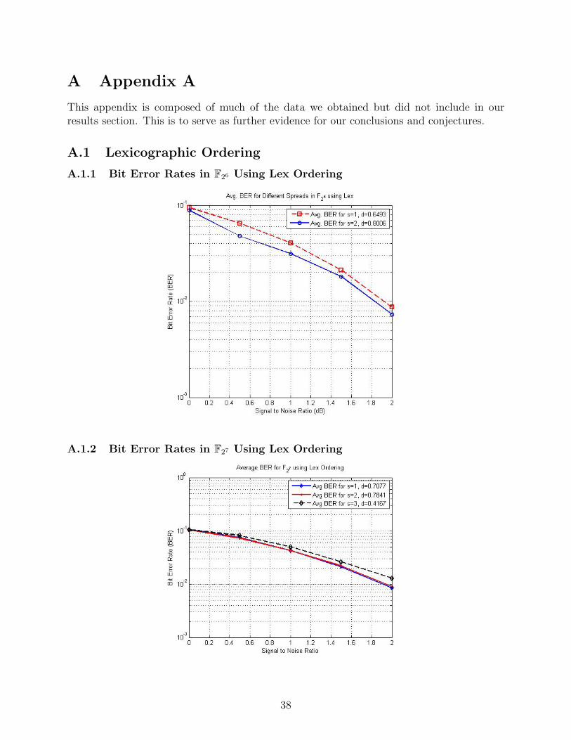
A Appendix A
This appendix is composed of much of the data we obtained but did not include in ourresults section. This is to serve as further evidence for our conclusions and conjectures.
A.1 Lexicographic Ordering
A.1.1 Bit Error Rates in F26 Using Lex Ordering
A.1.2 Bit Error Rates in F27 Using Lex Ordering
38

39
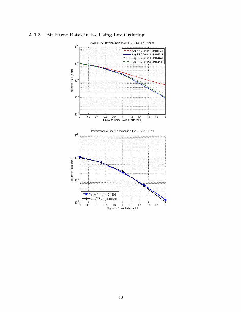
A.1.3 Bit Error Rates in F28 Using Lex Ordering
40

A.1.4 Bit Error Rates in F34 Using Lex Ordering
41

A.1.5 Bit Error Rates in F35 Using Lex Ordering
42
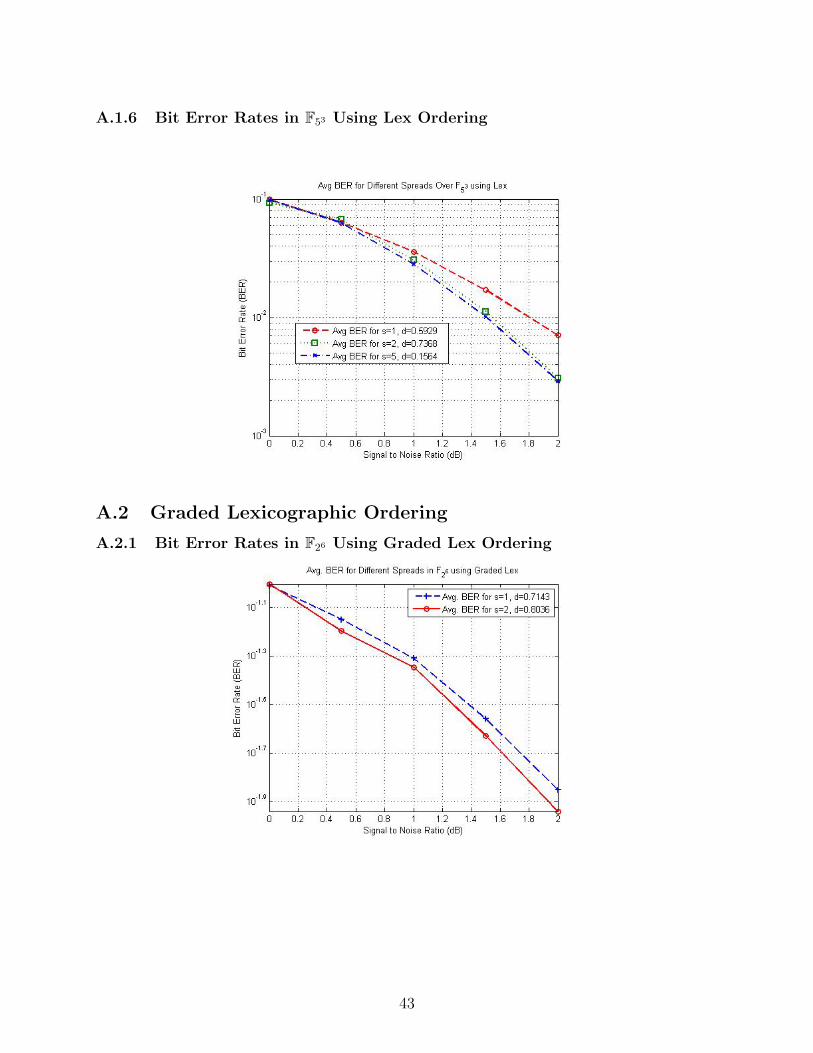
A.1.6 Bit Error Rates in F53 Using Lex Ordering
A.2 Graded Lexicographic Ordering
A.2.1 Bit Error Rates in F26 Using Graded Lex Ordering
43
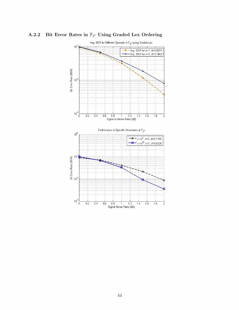
A.2.2 Bit Error Rates in F27 Using Graded Lex Ordering
44

A.2.3 Bit Error Rates in F28 Using Graded Lex Ordering
45

A.2.4 Bit Error Rates in F34 Using Graded Lex Ordering
46

A.2.5 Bit Error Rates in F53 Using Graded Lex Ordering
47

A.3 Graded Reverse Lexicographic Ordering
A.3.1 Bit Error Rates in F26 Using Graded Reverse Lex Ordering
48

A.3.2 Bit Error Rates in F27 Using Graded Reverse Lex Ordering
49
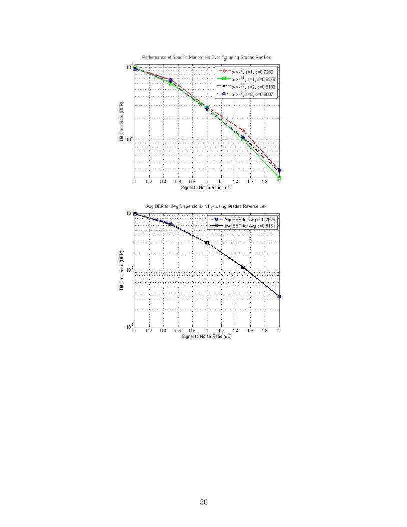
50

A.3.3 Bit Error Rates in F28 Using Graded Reverse Lex Ordering
51

A.3.4 Bit Error Rates in F34 Using Graded Reverse Lex Ordering
52

A.3.5 Bit Error Rates in F35 Using Graded Reverse Lex Ordering
A.3.6 Bit Error Rates in F53 Using Graded Reverse Lex Ordering
B Appendix B
B.1 A Note on Matlab Programs for this Project
These Matlab programs were all created during AMSSI 2006. Some of the programs dependon the Communications Toolbox developed for Matlab. Thus, these will not work on a nor-mal version of Matlab. The programs that will not work without the special toolbox will benoted in their beginning comments.
53

In all cases, the input of a permutation is given to a program as a vector of the imagesof the permutation. For example, the permutation
π =
(0 1 2 3 4 54 2 5 0 3 1
)would be passed to the program as the vector [4 2 5 0 3 1] (or, equivalently, [4,2,5,0,3,1]).
Additionally, polynomials such as 1+α2+α5 or 4+α+7α3 would be passed as [1 0 1 0 0 1]and [4 1 0 7], respectively, with the numbers in the vector representing the coefficients onthe powers of the polynomial variable, beginning with the variable to the 0th power as thefurthest left entry, and moving up by one power for each entry to the right. Though the pro-grams here are written specifically for monomials like xi, they can be fairly easily modifiedto accept polynomials with integer coefficients as the permutation polynomial. Some hintsfor this are given in the programs likely to be modified.
In addition to the titles of each program, it is important to read the first few lines of theprogram to examine its inputs and outputs. This will give a greater understanding of thenature of the program.
B.2 Programs Examining Properties of Permutations
B.2.1 Program to Determine Spread
This program takes a permutation as input and outputs the value of the spread.
function out=spread(vect)
%out=spread(vect)
% Calculates the spread of a permutation ’vect’
% Outputs the numeric value of the spread
% AMSSI 2006 - Mod 4 Armada
% Public Domain as long as above lines remain intact
out=1; % sets up default spread value
q=length(vect); % initialize variables
s=2;
flag=0;
while (s<=(sqrt(q/2)+2) && (flag~=1)) % sets conditions for ending loop
j=2;
% starts looping j upwards until it reaches the
% end of the vector or we find where s fails
while ((j<=q) && (flag~=1))
i=(j-(s-1)); % sets up i based on the value of s
if (i<=0) % moves i back to 1 if above line sends it 0 or less
i=1;
54

end
while ((flag~=1) && (i<j)) % starts looping i upwards until i<j s fails
if abs(vect(j)-vect(i)) < s % failure condition for s
flag=1;
out=s-1;
end
i=i+1;
end
j=j+1;
end
if flag~=1 % if flag was not tipped off, then all values of i,j for the
out=s; % specific s worked, so s is a new candidate for spread
end
s=s+1;
end
B.2.2 Program to Determine Spread Factors
function mini=permdist(perm)
%mini=permdist(perm)
% Calculates the spread factors of the permutation ’perm’
% Outputs the decimal value of the spread factor of ’perm’
% AMSSI 2006 - Mod 4 Armada
% Public Domain as long as above lines remain intact
n=length(perm);
mini=2*n; % set ’mini’ very large so it’s replaced in first loop
for i=1:n-1;
for j=i+1:n; % adds the ’distance’ between i and j, and
%% the ’distance between perm(i) and perm(j)
dist=min(mod(i-j,n),mod(j-i,n))+
min(mod(perm(i)-perm(j),n),mod(perm(j)-perm(i),n));
mini=min(dist,mini); % picks smallest between old min and new value
end
end
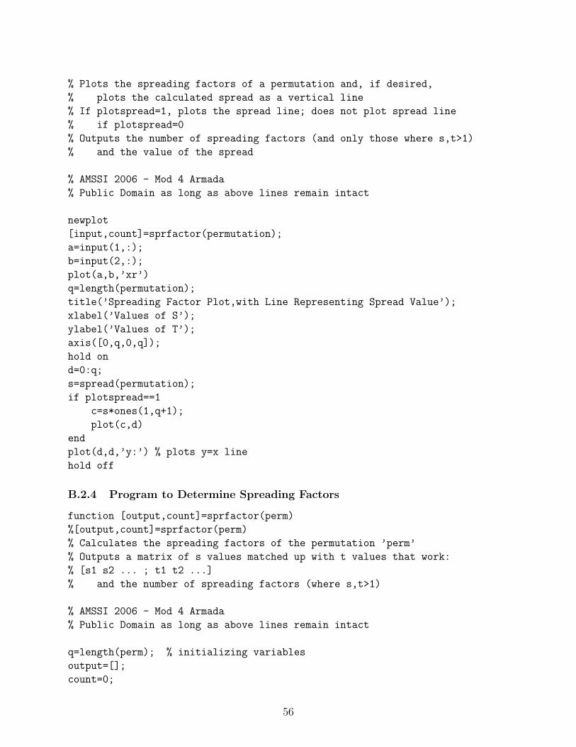
B.2.3 Program to Plot Spreading Factors
This program uses the above program to determine spreading factors, and then plots thosespreading factors. This also plots a yellow dotted y = x line for ease in finding the s-parameter. The program can also plot a line showing the calculated spread value for com-parison with the s-parameter, if the correct argument is passed.
function [count,s]=plotsprfactor(permutation,plotspread)
%[count,s]=plotsprfactor(permutation,plotspread)
55
% Plots the spreading factors of a permutation and, if desired,
% plots the calculated spread as a vertical line
% If plotspread=1, plots the spread line; does not plot spread line
% if plotspread=0
% Outputs the number of spreading factors (and only those where s,t>1)
% and the value of the spread
% AMSSI 2006 - Mod 4 Armada
% Public Domain as long as above lines remain intact
newplot
[input,count]=sprfactor(permutation);
a=input(1,:);
b=input(2,:);
plot(a,b,’xr’)
q=length(permutation);
title(’Spreading Factor Plot,with Line Representing Spread Value’);
xlabel(’Values of S’);
ylabel(’Values of T’);
axis([0,q,0,q]);
hold on
d=0:q;
s=spread(permutation);
if plotspread==1
c=s*ones(1,q+1);
plot(c,d)
end
plot(d,d,’y:’) % plots y=x line
hold off
B.2.4 Program to Determine Spreading Factors
function [output,count]=sprfactor(perm)
%[output,count]=sprfactor(perm)
% Calculates the spreading factors of the permutation ’perm’
% Outputs a matrix of s values matched up with t values that work:
% [s1 s2 ... ; t1 t2 ...]
% and the number of spreading factors (where s,t>1)
% AMSSI 2006 - Mod 4 Armada
% Public Domain as long as above lines remain intact
q=length(perm); % initializing variables
output=[];
count=0;
56
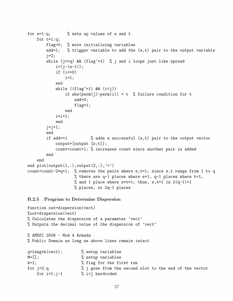
for s=1:q; % sets up values of s and t
for t=1:q;
flag=0; % more initializing variables
add=1; % trigger variable to add the (s,t) pair to the output variable
j=2;
while (j<=q) && (flag~=1) % j and i loops just like spread
i=(j-(s-1));
if (i<=0)
i=1;
end
while ((flag~=1) && (i<j))
if abs(perm(j)-perm(i)) < t % failure condition for t
add=0;
flag=1;
end
i=i+1;
end
j=j+1;
end
if add==1 % adds a successful (s,t) pair to the output vector
output=[output [s;t]];
count=count+1; % increases count since another pair is added
end
end
end plot(output(1,:),output(2,:),’+’)
count=count-2*q+1; % removes the pairs where s,t=1; since s,t range from 1 to q
% there are q-1 places where s=1, q-1 places where t=1,
% and 1 place where s=t=1; thus, s,t=1 in 2(q-1)+1
% places, or 2q-1 places
B.2.5 Program to Determine Dispersion
function out=dispersion(vect)
%out=dispersion(vect)
% Calculates the dispersion of a parameter ’vect’
% Outputs the decimal value of the dispersion of ’vect’
% AMSSI 2006 - Mod 4 Armada
% Public Domain as long as above lines remain intact
q=length(vect); % setup variables
M=[]; % setup variables
k=1; % flag for the first run
for j=2:q % j goes from the second slot to the end of the vector
for i=1:j-1 % i<j hardcoded
57

if (k==1) % M has no vectors, no reason to check the "other" pairs
M=[j-i;vect(j)-vect(i)];
k=2; % M now has values, must go to next section from now on
else
addin=1; % sets up flag to add pair into matrix
for l=1:length(M)-1 % checks matrix for the current ordered pair
if ((j-i)==M(1,l)) && ((vect(j)-vect(i))==M(2,l))
addin=0; % if the pair is found, must not add the pair in
end
end
if (addin==1) % pair was not found by code above, so it’s added
V=[j-i; vect(j)-vect(i)];
M=[M V];
end
end
end
end
[m,n]=size(M); % gets size of the matrix; want # columns
out=(2*n)/(q*(q-1)); % calculates the dispersion value
B.2.6 Optimized Program to Determine Dispersion
This is a much-improved version of the dispersion program that will run quite quickly com-pared with the last program.
function out=fastdisp(vect)
%out=fastdisp(vect)
% Calculates the dispersion of a parameter ’vect’
% Outputs the decimal value of the dispersion of ’vect’
% AMSSI 2006 - Mod 4 Armada
% Public Domain as long as above lines remain intact
q=length(vect);
M=zeros(q-1,2*q-1); % setup variables, (q-1)x(2q-1) matrix of zeros
for j=2:q % j from the second slot to the end of the vector
for i=1:j-1 % since i<j, start i at 1 then go to j-1
% changes component of matrix from 0 to 1 if
% calculated dispersion pair corresponding to the coordinates appears
M(j-i, vect(j)-vect(i)+q)=1 ;
end
end
%next line takes sum of matrix m, then the sum of the transpose,
58

% which gives cardinality of D, then plugs into dispersion formula
out=(2*sum(sum(M)’))/(q*(q-1));
B.2.7 Program to Determine Cyclic Decomposition Cycles
function output=decomposition(vect)
%output=decomposition(vect)
% Calculates the cyclic decomposition of the input permutation ’vect’
% Outputs a matrix containing the n-cycles and how many times each appears
% ie, 1 3 6
% 4 1 2
% represents 4 1-cycles, 1 3-cycle, and 2 6-cycles
% AMSSI 2006 - Mod 4 Armada
% Public Domain as long as above lines remain intact
tester=sort(vect); % the next three lines make sure program operates correctly
offset=tester(1); % only works w/perms that contain 0; thus, sorts input vector,
vect=vect-offset; % looks first (now smallest) entry, offsets the vector by that
q=length(vect); % next five lines set up the intial values of variables
counter=[];
used=[];
index=1;
cycle=[];
while(length(used)<q)
k=index-1; % accounts for the off-by-one
while(k~=vect(index)) % cycles through the perm until back to index value
cycle=[cycle vect(index)];
used=[used vect(index)];
index=vect(index)+1;
end
cycle=[cycle vect(index)]; % since cycle added pi(index) as first element,
%% we must specially add in the original index
used=[used vect(index)];
counter=[counter length(cycle)];
used=sort(used); % preps for comparison below
i=0;
while (i<length(used)) && (i==used(i+1)) % find the first index not used
i=i+1;
end
index=i+1;
cycle=[]; % resets the cycle to empty matrix to begin loop again
end
counter=sort(counter); % sorts to expedite creation of the output vector
59

output=[];
for k=1:length(counter) % following loop goes adds element to counter if unique
marker=0; % or increases tally if element is not unique
l=1;
[m,n]=size(output);
while (marker==0) && (l<=n)
if counter(k)==output(1,l)
variable=output(2,l);
output(2,l)=(output(2,l)+1);
marker=1;
end
l=l+1;
end
if marker==0
output=[output [counter(k);1]];
end
end
B.3 Field Arithmetic Programs
B.3.1 Program to Evaluate Addition in a Field
This program to add in a field Fpn uses the function gfadd, which is available only in theMatlab Communications Toolbox.
function output=gfaddition(alpha,num,field)
% output=gfaddition(alpha,num,field)
% Performs additions of variables in a Galois Field called ’field’
% adding ’alpha’ to itself ’num’ times
% One example is 2(alpha)^3; num=2 in this case
% AMSSI 2006 - Mod 4 Armada
% Public Domain as long as above lines remain intact
output=alpha; % sets up default alpha value
% (won’t enter loop if num=1)
for i=1:num-1 % loops up to the correct number of additions
output=gfadd(output,alpha,field);
end
B.3.2 Program to Evaluate Exponents in a Field
This program to evaluate exponents in a field Fpn uses the function gfmul, which is availableonly in the Matlab Communications Toolbox.
function
60

powr=gfexpo(num,i,field)
%powr=gfexpo(num,i,field)
% Evaluates exponents in a Galois Field, taking a field element num^i by
% multiplying it by itself i times
% ie, (alpha)^6 --> num=alpha, i=6
% AMSSI 2006 - Mod 4 Armada
% Public Domain as long as above lines remain intact
if i==0 % hard codes the basic default case
powr=0;
else
powr=num;
for j=1:i-1 % loop multiplies num times itself i-1 times
powr=gfmul(powr,num,field);
end
end
B.3.3 Program to Evaluate Polynomials in a Field
This program to calculate values plugged into a polynomial in a field Fpn uses the functionsgfadd, gfexpo, and gfaddition, which are available only in the Matlab CommunicationsToolbox.
function output=gfpoly(num,vect,field)
%output=gfpoly(num,vect,field)
% Program to evaluate plugging variables like (alpha)^6 into polys like 1+x+x^2
% In the example, num=(alpha)^6 and vect=[1 1 1] (which represents 1+x+x^2)
% Outputs the value of the evaluated polynomial
% AMSSI 2006 - Mod 4 Armada
% Public Domain as long as above lines remain intact
output=-Inf; % default output; evaluates to 0 in any field
for j=1:length(vect) % sets up loop to step through every part of vector
exponen=gfexpo(num,j-1,field); % calls exponent to evaluate num to power
if vect(j)==0 % default value if any element of the vector is 0
added=-Inf;
else
% adds up the exponentiated alphas to deal with coeffiecients
added=gfaddition(exponen,vect(j),field);
end
output=gfadd(output,added,field); % adds new (alpha)^x value to previous add’ns
end
61

B.4 Random Necessary Programs
B.4.1 Program to Determine Base Representations
This program takes in a decimal number and a prime power pn, and calculates the number’srepresentation in the new base.
function vect=baserep(num,p,n)
%vect=baserep(num,p,n)
% Calculates the base p representation of a decimal number ’num’ up to
% n digits
% Outputs the base representation of the number as a vector
% AMSSI 2006 - Mod 4 Armada
% Public Domain as long as above lines remain intact
digs=n; % calculates # of digits required in the end number
vect=[];
for j=1:digs % loops through every digit
temp=mod(num,p); % evaluate mod of number, then
vect=[vect temp]; % add to vector, then
num=(num-temp)/p; % subtract the mod off the original and loop back
end
B.4.2 Program to Generate Random Integer
There is a built-in program, randint, which is available only in the Matlab CommunicationsToolbox. In order to use this program on other computers without the Toolbox, we had tocopy the code to a separately named Matlab program file.
B.5 Sorting Programs
B.5.1 Program to Sort a Set of Vectors
This program requires that the vectors be stored as columns of a matrix. Example: to sort
[1 2 3], [8 3 2], and [0 9 3], they should be passed to the program as M =
1 8 02 3 93 2 3
.
function data=selectionsort(M,data,first)
%data=selectionsort(M,data,first)
% Sorting algorithm based on swapping the largest value into the last slot,
% then moving the "last" slot up by one and repeating
% M ~ Monomial ordering;
% data ~ vector of items that need sorting;
% first ~ the first index where sorting should begin
62
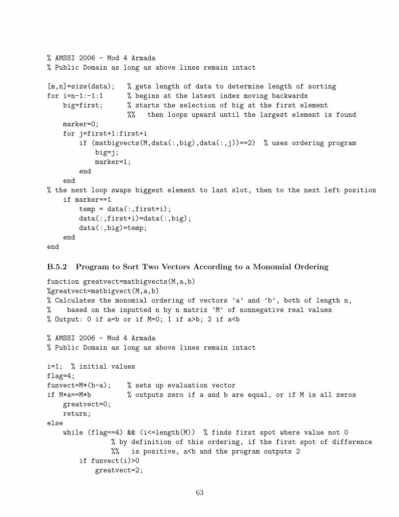
% AMSSI 2006 - Mod 4 Armada
% Public Domain as long as above lines remain intact
[m,n]=size(data); % gets length of data to determine length of sorting
for i=n-1:-1:1 % begins at the latest index moving backwards
big=first; % starts the selection of big at the first element
%% then loops upward until the largest element is found
marker=0;
for j=first+1:first+i
if (matbigvects(M,data(:,big),data(:,j))==2) % uses ordering program
big=j;
marker=1;
end
end
% the next loop swaps biggest element to last slot, then to the next left position
if marker==1
temp = data(:,first+i);
data(:,first+i)=data(:,big);
data(:,big)=temp;
end
end
B.5.2 Program to Sort Two Vectors According to a Monomial Ordering
function greatvect=matbigvects(M,a,b)
%greatvect=matbigvect(M,a,b)
% Calculates the monomial ordering of vectors ’a’ and ’b’, both of length n,
% based on the inputted n by n matrix ’M’ of nonnegative real values
% Output: 0 if a=b or if M=0; 1 if a>b; 2 if a<b
% AMSSI 2006 - Mod 4 Armada
% Public Domain as long as above lines remain intact
i=1; % initial values
flag=4;
funvect=M*(b-a); % sets up evaluation vector
if M*a==M*b % outputs zero if a and b are equal, or if M is all zeros
greatvect=0;
return;
else
while (flag==4) && (i<=length(M)) % finds first spot where value not 0
% by definition of this ordering, if the first spot of difference
%% is positive, a<b and the program outputs 2
if funvect(i)>0
greatvect=2;
63

flag=7;
% by definition of this ordering, if the first spot of difference
%% is negative, a>b and the program outputs 2
elseif funvect(i)<0
greatvect=1;
flag=5;
end
i=i+1; % if the vectors don’t differ at i, loops to the next slot
end
end
B.5.3 Program to Output a Graded Lexicographic Matrix Representation
function matrix=grlex(size)
%matrix=grlex(size)
% Creates a ’size’ by ’size’ matrix that will represent
% a graded lexicographic ordering when used
% in the vector ordering program
% Outputs a ’size’ by ’size’ matrix
% AMSSI 2006 - Mod 4 Armada
% Public Domain as long as above lines remain intact
% first row is all 1s;
% bottom part is a lex matrix with the last row cut off
matrix=[ones(1,size); eye(size-1,size)];
B.5.4 Program to Output a Graded Reverse Lexicographic Matrix Represen-tation
function matrix=grevlex(size)
%matrix=grevlex(size)
% Creates a ’size’ by ’size’ matrix that will represent
% a graded reverse lexicographic ordering when used
% in the vector ordering program
% Outputs a ’size’ by ’size’ matrix
% AMSSI 2006 - Mod 4 Armada
% Public Domain as long as above lines remain intact
matrix=[ones(1,size)]; % Top row of grevlex matrix
temp=eye(size-1,size); % Sets up bottom part of grevlex
temp=abs(temp-1); % Switches zeros and ones
i=1;
j=size;
64
% Flips columns of the temp to reverse direction of the zero diagonal
while (i<j)
temp2=temp(:,i);
temp(:,i)=temp(:,j);
temp(:,j)=temp2;
i=i+1;
j=j-1;
end
matrix=[matrix;temp]; % Combines upper and lower parts
B.6 Permutation Calculation Programs
B.6.1 Program to Calculate a Permutation in a Field, Using a Specified Order-ing and Permutation Polynomial
This program uses a number of programs that depend on the Matlab Communications Tool-box.
function output=monomialordermap(M,p,n,j)
%output=monomialordermap(M,p,n,j)
% Calculates the resulting permutation in Z_p^n using monomial ordering ’M’,
% in field of size p^n, and the center permuting polynomial x^j
% Outputs the resulting permutation in vector form
% AMSSI 2006 - Mod 4 Armada
% Public Domain as long as above lines remain intact
%% Goes from Z(p^n) to (Zp)^n, sorts according to monomial order M
%% (ex: from integers to polynomials sorted by lex)
vect=num2vect(M,p,n);
conversion=vect; % stores conversion matrix for later
%% Defines the field we are working in
field=fielddefine(p,n);
%% Runs the polynomials (in terms of alpha) through a permutation, which
%% can itself be a polynomial
[c,d]=size(vect);
output=[];
for i=1:d
65

[tp,expform]=gftuple(vect(:,i)’ ,n,p); % converts from (Zp)^n to F(p^n)
output=[output gfexpo(expform,j,field)];
end
vect=output;
%% Converts the output in F(p^n) back into (Zp)^n
output=[];
for i=1:d
[tp,expform]=gftuple(vect(i),n,p); % converts from F(p^n) to (Zp)^n
output=[output;tp];
end
vect=output’;
%% Converts the vector into Z(p^n)
output=vect2num(conversion, vect);
For working with polynomials that not are simple monomials the following changes canbe made:
(i) The first few lines of the program can be replaced with:
function output=monomialordermap(M,p,n,permutation)
%output=monomialordermap(M,p,n,permutation)
% Calculates the resulting permutation in Z_p^n using monomial ordering ’M’,
% in field of size p^n, and the center permuting polynomial ’permutation’
% with integer coefficients
(ii) In the middle of the program, the lines where the polynomials are run through thepermutation, the lines can be replaced with:
for i=1:d
[tp,expform]=gftuple(vect(:,i)’,n,p); % converts from (Zp)^n to F(p^n)
output=[output gfpoly(expform,permutation,field)];
end
(Note that this modified version requires modifications of the programs on which monomi-alordermap depends to accept arguments of polynomials, described as vectors, instead ofjust an i-value.)
B.6.2 Program to Take the Elements of Zpn Into (Zp)n, and Order Them by a
Monomial Ordering
function vect=num2vect(M,p,n)
66

% vect=num2vect(M,p,n)
% Creates a list of ordered vectors in the specified base p^n
% using the elements of Z(p^n), converting them to (Zp)^n,
% then sorting the resulting elements of (Zp)^n
% Outputs a sorted vector of elements of (Zp)^n
% AMSSI 2006 - Mod 4 Armada
% Public Domain as long as above lines remain intact
vect=[];
for i=0:(p^n)-1 % adds all numbers from 0 to base-1 to a vector
vect=[vect;baserep(i,p,n)];
end
vect=vect’; % transposes the vector so it sorts correctly
vect=selectionsort(M,vect,1);
B.6.3 Program to Take the Elements of (Zp)n Back Into Zpn Using the a Specified
Conversion Ordering
function permvect=vect2num(Q,H)
% permvect=vect2num(Q,H)
% Takes in the conversion table from the num2vect and list of outputted
% vectors from the permutation
% Q ~ conversion factor matrix;
% H ~ result of the previous step
% Outputs the converted integers
% AMSSI 2006 - Mod 4 Armada
% Public Domain as long as above lines remain intact
[m,n]=size(H);
permvect=zeros(1,n); % sets up vector that ends up outputting integers in order
for i=1:n % loops through the permutation vectors
for j=1 % loops until conversion table and perm vectors match
while ~isequal(H(:,i),Q(:,j))
j=j+1;
end
end
permvect(i)=j-1; % adds integer value to specified spot in output vector
end
B.6.4 Program to Define the Working Field
This program to calculate a field Fpn uses the function gftuple, which is available only inthe Matlab Communications Toolbox.
67

function field=fielddefine(p,n)
%field=fielddefine(p,n)
% Method for constructing a field of size p^n and outputting the
% proper variable, ’field’, for future use
% AMSSI 2006 - Mod 4 Armada
% Public Domain as long as above lines remain intact
field = gftuple([-1:p^n-2]’,n,p); % Constructs list of elements.
B.7 Permutation Creation Programs
B.7.1 Program to Create Permutations in a Field Fpn using a Monomial Order-ing and to Calculate Measurements of Each Permutation
This program depends on a program that utilizes elements in the Matlab CommunicationsToolbox.
function
[permutation,isperm,sprd,dispers,cyclic,sprdfactor]=allofit(M,p,n,i)
%[permutation,isperm,sprd,dispers,cyclic]=allofit(M,p,n,poly)
% Determines if a polynomial is a permutation, and returns the spread,
% dispersion, and cyclic decomposition if the polynomial is a permutation.
% Where M=Matrix describing monomial order, p=base, n=exponent (ie, p^n),
% and poly=polynomial to be used
% Outputs the permutation; isperm=1 if poly is a permutation, 0 if not;
% spread; dispersion; and cyclic decomposition
% AMSSI 2006 - Mod 4 Armada
% Public Domain as long as above lines remain intact
permutation=monomialordermap(M,p,n,i); % permutation creation
isperm=testperm(permutation,p,n); % tests if a permutation
if (isperm==1) % calcs and stores measures of a perm
sprd=spread(permutation);
dispers=dispersion(permutation);
cyclic=decomposition(permutation);
sprdfactor=permdist(permutation);
else
sprd=‘error - your permutation sucks’;
dispers=‘error - your permutation sucks a lot’;
cyclic=‘error - why oh why did you pick that permutation’;
sprdfactor=‘error - even the spread factors hate your permutation!’;
end
68
B.7.2 Program to Test if a Candidate is a Permutation
function output=testperm(perm,p,n)
%output=testperm(perm,p,n)
% Tests a candidate to see if it is a permutation
% Outputs 1 if the candidate is a permutation, 0 if it is not
% AMSSI 2006 - Mod 4 Armada
% Public Domain as long as above lines remain intact
output=1;
flag=0;
perm=sort(perm);
i=0;
% after sorting, the vector is in ascending order starting at zero,
% so the loop starts i at zero and checks to make sure that the ith
% slot of the sorted permutation equals i
while (flag==0) && (i<p^n)
if i~=perm(i+1)
output=0;
flag=1;
end
i=i+1;
end
B.8 Permutation Determination, Storage, and Retrieval Pro-grams
B.8.1 Program to Calculate Measurements for Permutations in a Field
function allinone(M,p,n,filename)
%allinone(M,p,n,print)
% Determines whether each of the polynomials making up the field are a
% permutation, and prints out the spread, dispersion, and cyclic
% decomposition of the polynomials.
% M ~ Matrix determining monomial ordering (dimensions n by n)
% p ~ prime number
% n ~ power of prime number (p^n makes up the order of the field, ie F_p^n)
% print ~ type 1 to print out poly, sprd, disp, and decomp for each
% polynomial even if not a permutation, type 0 to just print the
% information for polynomials that are permutations
% AMSSI 2006 - Mod 4 Armada
% Public Domain as long as above lines remain intact
69

perms=[];
ivalues=[];
ordering=M;
spreads=[];
dispersions=[];
sprdfactors=[];
for i=0:(p^n-1) % loop to set up, calc all the p^n polys w/integer coeff
if (gcd(i,(p^n-1))==1)
% calls the allofit function to check whether each polynomial generates a
% permutation; if it does, the next lines output the relevant values
[per,isperm,sprd,disp,decomp,sprdfactor]=allofit(M,p,n,i);
i
per;
sprd;
disp;
decomp;
sprdfactor;
perms=[perms;per];
ivalues=[ivalues;i];
spreads=[spreads; sprd];
dispersions=[dispersions; disp];
sprdfactors=[sprdfactors; sprdfactor];
end
end
% setup to store variables
% perms must have 1 added to accomodate turbo_simulator
polys=ivalues;
perms=perms+1;
save(filename,’polys’,’perms’,’ordering’,’spreads’,’dispersions’,’sprdfactors’)
B.8.2 Program to Read Measurements from a Field File
function [po,or,sp,di,sf]=readallinonemeasures(filename)
%[po,or,sp,di,sf]=readallinonemeasures(filename)
% Reads the stored polynomials, ordering, spreads, dispersions, and spread
% factors from a specified field file.
% Outputs five variables to that contain the polynomials, the ordering, the
% spreads, the dispersions, and the spread factors in that order.
% AMSSI 2006 - Mod 4 Armada
% Public Domain as long as above lines remain intact
load(filename,’polys’,’ordering’,’spreads’,’dispersions’,’sprdfactors’)
po=polys; % the next five lines set the return variables
70
or=ordering;
sp=spreads;
di=dispersions;
sf=sprdfactors;
B.8.3 Program to Read Permutations from a Field File
function [po,pe]=readallinoneperm(filename)
%[po,pe]=readallinoneperm(filename)
% Reads the stored polynomials and permutations from a specified field file.
% Outputs two variables to that contain the polynomials and the
% permutations, in that order.
% AMSSI 2006 - Mod 4 Armada
% Public Domain as long as above lines remain intact
load(filename,’perms’,’polys’)
pe=perms;
po=polys;
B.9 Interleaver Simulation Programs
B.9.1 Program to Run Multiple Simulations on a Field File
function simfromfile(filename,nums)
%simfromfile(filename,nums)
% Runs specified number of simulations, ’nums’, on the field file.
% Saves simulation data for each permutation to an extended version of the
% original name; ie, for lex_f2_2, one might be saved as lex_f2_2_2.
% AMSSI 2006 - Mod 4 Armada
% Public Domain as long as above lines remain intact
load(filename,’perms’) m=length(nums);
a=readallinonemeasures(filename)’ % gets all i values
for i=1:m
% j loop finds index where each i value is located
for j=1:length(a)
if nums(i)==a(j)
use=j;
nums(i);
end
end
% creates extended filename, and runs the specified simulation
filei=[filename,’_’,num2str(nums(i))];
71
turbo_simulator(perms(use,:),filei);
end
B.9.2 Program to Read Bit Error Rates from a Field File
This program can only be run after successful simulation of the permutations. It also requiresthat all the files associated with the field file be in the same directory as the original fieldfile. Example: After simulating lex f2 2, you may have the associated field files lex f2 2 1and lex f2 2 2. The latter files must be in the same directory as the original field file for thisprogram to work.
function output=readber(filename,ivect)
%output=readber(filename,ivect)
% Reads the specified Bit Error Rates from a field file.
% filename ~ name of field file
% ivect ~ vector listing requested i-values
% Outputs requested Bit Error Rates
% AMSSI 2006 - Mod 4 Armada
% Public Domain as long as above lines remain intact
q=length(ivect);
output=zeros(q,5);
for i=1:q % loops through the i values and stores the BERs for output
filei=[filename,’_’,num2str(ivect(i))];
load(filei,’ber’);
output(i,:)=ber(:,length(ber))’;
end
B.9.3 Program to Graph Specified Bit Error Rates
function ber_graph(filename,ivect,len)
%ber_graph(filename,ivect,len)
% Graphs the specified BERs for each signal to noise ratio
% filename ~ filename to get data from
% ivect ~ specifies which values of x^i to plot
% len ~ hack to make legend come out right; this is the number
% of digits of the highest i-value
% AMSSI 2006 - Mod 4 Armada
% Public Domain as long as above lines remain intact
newplot
q=length(ivect);
hold on % needed to graph multiple graphs; gets this done early on
legi=[];
72

color=[’y’ ’m’ ’c’ ’r’ ’g’ ’k’]; % vectors that set up matlab line styles
line=[’-’,’:’,’-.’,’--’];
style=[’.’ ’o’ ’x’ ’+’ ’s’ ’d’ ’v’ ’^’ ’p’ ’h’ ’<’ ’>’];
for i=1:q
filei=[filename,’_’,num2str(ivect(i))]; % ith filename created
load(filei,’EbN0db’,’ber’) % loads BERs from the ith file
[m,n]=size(ber);
EbNoveci=EbN0db; % vector of signal to noise ratios
BERveci=ber(:,n);
% the randint program is in the Matlab Communications Toolbox, so one would
% have to create his or her own version to run the next three lines
l = randint(1,1,[1,length(line)]); % picks random style
s = randint(1,1,[1,length(style)]);
c = randint(1,1,[1,length(color)]);
plotsym= [style(s) line(l) color(c)]; % random plotstyle for this curve
semilogy(EbNoveci,BERveci,plotsym); % actually plots curve
tempvect=num2str(ivect(i));
p=length(tempvect);
if p~=len % creates line in legend for each line graphed
for j=p:len-1
tempvect=[tempvect,’‘’]; % add in hack to make legend work
end
end
addin=strcat(’x->x^’,tempvect);
legi=[legi;addin];
end
% adds in graph axis labels, title, and legend
grid on;
title(’Performance of Turbo Codes Using Monomial Permutations’);
xlabel(’Signal to Noise Ratio (EbNo (dB))’);
ylabel(’Bit Error Rate (BER)’);
legend(legi,’Location’,’Southwest’);
hold off
B.10 Programs to Create and Examine Semi-Random Permuta-tions
B.10.1 Program to Generate a Semi-Random Permutation
function perm=randomp(s,q)
%perm=randomp(s,q)
73

% input s and q, s=desired spread, q=field size
% AMSSI 2006 - Mod 4 Armada
% Public Domain as long as above lines remain intact
perm=zeros(1,q); % a 1xq zero matrix
available=ones(1,q); % available possibilities to choose from
pofflimits=zeros(1,q); % values off limits permanently
entry=randint(1,1,[1,q]); % picks a random number to insert into perm
perm(1)=entry; % randomly picks perms first entry without restrictions
for i=2:q
available(entry)=0; % changes indices of available matrix to 0
pofflimits(entry)=1; % changes pofflimits indices to 1
offlimits=pofflimits; % sets offlimits to pofflimites
max1=max(1,i-(s-1)); % next 2 lines pick range to test spread
w=perm(max1:i-1);
% enter things into offlimits by test spread, dist from other things
for j=1:length(w)
max2=max(1,w(j)-(s-1));
min1=min(q,w(j)+(s-1));
offlimits(max2:min1)=1;
end
available=ones(1,q)-offlimits; % subtract the ones from offlimits
v=find(available==1); % finds spaces in available equal to 1
if isempty(find(v)), break, end; % tests to see if there are availables
e=randint(1,1,[1,length(v)]); % picks randint between 1, length avaiables
entry=v(e); % makes entry the index of random integer
perm(i)=entry; % puts this into perm
end
B.10.2 Program to Keep Searching for a Semi-Random Permutation
function permy=reallyrandomp(s,q)
%permy=reallyrandomp(s,q)
% Runs really random p until it makes a real permutation
% Outputs an actual semi-random perm
% AMSSI 2006 - Mod 4 Armada
% Public Domain as long as above lines remain intact
flag=0;
while flag==0
permy=randomp(s,q);
if ~(permy(q)==0)
74

flag=1;
end
end
B.10.3 Program to Simulate Random Permutation
function storereallyrandomp(s,q,filename)
%storereallyrandomp(s,q,filename)
% Runs turbo_simulator with generated semi-random permutation
% Stores information in specified filename
% - use readberrandom to retrieve information
% AMSSI 2006 - Mod 4 Armada
% Public Domain as long as above lines remain intact
perm=reallyrandomp(s,q)
turbo_simulator(perm,filename);
B.10.4 Program to Retrieve Information from a Simulated Permutation
function readberrandom(filename)
%output=readberrandom(filename,ivect)
% Reads the specified Bit Error Rates from a field file
% created by a random permutation.
% filename ~ name of field file
% Outputs requested Bit Error Rates
% AMSSI 2006 - Mod 4 Armada
% Public Domain as long as above lines remain intact
output=zeros(1,5); % preallocating output vector
load(filename,’ber’,’alpha’); % load bit error rates
[m,n]=size(ber); % get size of BER matrix
output(1,:)=ber(:,n)’; % set up correct outputs
% lines print permutation, spread, dispersion, sprfactor to screen
perm=alpha
spr=spread(alpha)
disp=dispersion(alpha)
sprfact=permdist(alpha)
permber=output
B.10.5 Program to Examine Dispersions of Random Permutations
function d=randomdispersionloop(s,q,goes)
%d=randomdispersionloop(s,q,goes)
75

% Creates several permutations of a given spread and field size, then
% computes the dispersion.
% s=spread, q=field size, goes=# of permutations
% AMSSI 2006 - Mod 4 Armada
% Public Domain as long as above lines remain intact
d=zeros(1,goes); %initial dispersion matrix as zeros
for k=1:goes %runs specified amount of times
%calculates dispersions of perms generated, outputs as vector
d(k)=fastdisp(reallyrandomp(s,q));
end
76