aldo bischi, ph.d. a.bischi@skoltech · associate characteristic curves to each unit, ... start-up)...

March, 2012 |

Combined cooling, heat and power systems operation planning & design:

Mixed Integer Non Linear Programming

Aldo Bischi, Ph.D. [email protected]

15h September, 2016

Contents

➜Combined Cooling, Heat and Power (CCHP) Generation

➜CCHP Scheduling Optimization

CCHP Units characterization

Conceptual Lay out

Problem Statement: Mixed Integer Non Linear Problem (MINLP)

Startup & Shutdown Constraints

Yearly Problem

➜Design optimization

➜Future Plans

➜Test Case: Daily

http://www.gecos.polimi.it/

Combined Heat and Power (CHP)

Rational use of primary energy generating simultaneously heat,

electric/mechanical power

Fuel

Fcog

Prime Mover

Electric Energy

EE

Heat Q

Losses e.g. 10÷25%

EE

Q

Power Plant

Boiler

Fuel

FEE

Fuel

FQ

CHP

EE

Conventional

Losses

e.g. up to 10%

Large!!Losses Power generation & Transport

e.g. 40÷60%

Combined Cooling, Heat and Power (CCHP)

…..and refrigeration effect

Effective way to reduce Primary Energy consumption & CO2 emissions

Advantageous for Electric Power Distribution system,

No Construction of New Large Power Plants & High Voltage Network

Reliability, Peakshaving, Power quality, liberalization of electricity market

Fuel 100Prime

Mover

10Heat 55

Heat Losses 10

Absorption

ChillerCooling Load 38

Heat Losses 17

Example

Total

Efficiency

73%

Electric Power 35

Technologies: Size & Application Families

Load/Customer

Micro, 50kWel

Small Scale, < 1MWel

Large Scale

”Non-Standard” loads

Family (e.g. 1kWel), Small industries/Artisans

…eventually with large variations ► Unforeseeable

“Standard” loads:

Several Families, Tertiary sector, Small industries/Artisans, ► Foreseeable

District Heating/Cooling

Extra challenges due to both pressure & thermal load losses

Industrial Processes, Case-Specific!

- Temperature the heat is required

- N° of Temperature levels the heat is required

- Thermal loads small dependency on the season

Eventually unforeseeable!

► e.g. Oil & Gas,

Project SNAM Recompression Power Stations

(Large size & small number e.g. <200 units represent > 20% of Italian Th.Power, about 75GW)


Electric efficiency

Power Plant Size [kW]

Ele

ctri

c E

ffic

ien

cy [

%]

0 1 10 100 1000 104 105 106

0

10

20

30

40

50

60

70

80

Fuel Cells (FC)

Stirling

Engine

Hybrid Cycles FC + Gas

Turbine

Thermo Photo

Voltaic

Micro-turbine

Combined

cycles

USC e

IGCC

TG Aero

Derivative

Steam

Cycle

TG Heavy Duty

SOFC

Internal Combustion

Engine

Small Scale

….Distributed Power Generation

Large Scale …Industrial, District Heating

Micro-Cogeneration


(Electric & Thermal efficiency)

e.g. Small and Micro CHP

0 10 20 30 40 50 60 70 80 90 1000

10

20

30

40

50

60

70

80

90

100

Thermal Efficiency [%]

Ele

ctri

c E

ffic

ien

cy [

%]

Micro Gas Turbine

Internal Combustion Engine

Fuel Cells PAFC and PEM

Fuel Cells, MCFC and SOFC

Stirling Engine

Thermo Photo Voltaic

Limit Primary Energy Savings

PES = 0 (below 1MW)

e.g....10 for Power plants above 1MW

100)QE

E1(PES

refth,

rec

prefel,

el

fuel

+

-=

hh

CCHP Challenges

Larger Investment Costs

Not Simultaneous Request of Electric Power & Heat

Bureaucracy & deep knowlege of the Legislation, Gas & Power Tarifs

Vary on hourly basis & depend on monthly/yearly consumption!

Temperature Level ......

Different Level ► Different Unit & Thermal Efficiency

More than one Level/Downgrade

Storage…Thermal/Cooling Load Power!

Optimal Design & Scheduling

Co-generative Units Characterization,

~

FPM

𝑸 GTcog

WelGTgen

1)

2) 3)

4)

5)

𝜂𝑐𝑜𝑚𝑏

𝜂𝐻𝑒𝑎𝑡𝐸𝑥𝑐ℎ

ℎ𝑖𝑛 = 𝑐𝑝 ∙ 𝑇𝑖𝑛 [kJ/kg K]

ℎ𝑜𝑢𝑡 = 𝑐𝑝 ∙ 𝑇𝑜𝑢𝑡 [kJ/kg K]Air

Exhausts

Water

𝑸GTcog

WelGTgen

FPM Prime Mover

(PM)

For several Ambient Temperatures

For several Fuel input, from Minimum to Nominal load

= 𝑚 ∙ Δℎ𝑖𝑛−𝑜𝑢𝑡[kW]

FSFFSF

Associate characteristic curves to

each unit, taking into consideration

just the fluxes in & out.

➜Experimental Measurements

➜Thermodynamic cycle calculation (each point),

High Level of Detail for Units Characterization

Nominal Conditions

Pel:1961kWel

T [⁰C]Fuel [kW]

Ele

ctri

cP

ow

er[k

W]

75%50%

100%

Gas Turbine Pratt & Whitney ST18A

“Two-degrees-of-freedom” units

~

FGT

EGT

𝑸GT,HT 𝑸LT,LT

+

𝑸GT,SF,N,cog,HT

FGT,SF,N,cogTemperature [°C]

FGT [kW] 𝑸

GT

,HT

&

𝑸G

T,S

F,N

,co

g,H

T[k

W]

40

-2010

FGT,SF,N,cog

“Three-degrees-of-freedom” units

e.g. Natural Gas Combine Cycle with Post Firing

~

FGT

Wel,GT

FGT,PF

~

HRSG

Vbleed

1st

.

2nd

3rd 𝑸

Wel,ST

𝑸 = 𝒇(FGT ,FGT,PF ,Vbleed)

Post Firing (PF)

Gas Turbine (GT)

Steam Turbine (ST)

Heat Recovery Steam Generator (HRSG)

𝑾𝒆𝒍,𝑮𝑻 = 𝒇(FGT )

𝑾𝒆𝒍,𝑺𝑻 = 𝒇(FGT ,FGT,PF ,Vbleed)

vs. “White Box” approach!

“Three-degrees-of-freedom” units

e.g. Natural Gas Combine Cycle with Post Firing

Valve

Opening

Fuel Post Firing [kW]Fuel [kW]

Ele

ctri

c P

ow

er [

kW

]

Simulation performed with https://www.thermoflow.com/

0 [kWh]

4,5 x 104[kWh]

Per Ambient Temperature[⁰C]!

https://www.thermoflow.com/

Performance curves NON Smooth

…..e.g. gas turbine (depends on the control strategy)

“Natura non facit saltus”….sometimes yes, but it is unusual

e.g. Solid Oxyde Fuel Cell (SOFC)

Non-Concave Functions

0

200

400

600

800

1000

1200

0 1000 2000 3000 4000

LT Heat

0

500

1000

1500

2000

2500

0 1000 2000 3000 4000

Electric Power

Original Source, https://www.bluegen.net/

[W]

[W]

Fuel input [W]

Fuel input [W]

https://www.bluegen.net/

Performance curves highly NON Linear

……..e.g. Heat Pump/Part Load

0

0,2

0,4

0,6

0,8

1

1,2

0 0,2 0,4 0,6 0,8 1

Low

Te

mp

era

ture

He

at

rela

tive

to

th

e n

om

ina

l [-]

Electric Power Consumption Percentage [%]

1 interval

2 intervals

Non Linear Curve

Condenser

Evaporator

45°C

Usefull

Effect

Y = (X1 ,X1)

Air vs.

Water

ElectricPower, X1

Performance Strong Temperature Dependency

Air Cooled Heat Pump

Evaporator Temperature = Tamb,

NOT a variable

Tamb reduction►• < cycle efficiency

• < mass flow compressor

0

0,1

0,2

0,3

0,4

0,5

0,6

0,7

0,8

0,9

1

1,1

1,2

-20 -10 0 10 20 30

Val

ue

s re

lati

ve t

o t

he

no

min

al [

-]

Ambient Temperature [°C]

COPAbsorbed Electric energy, Full Load

Scheduling Application

➜……..e.g. Heat Pump/Evaporator Temperature

Performance Strong Temperature Dependency

Water cooled Heat Pump

Evaporator Temp,

may receive heat from CHP system

► «two-degrees-of-freedom»!!

Condenser

Evaporator

45°CUsefull Effect

Y = (X1 ,X1)

Air vs. Water

ElectricPower, X1

RecoveredHeat, X2

➜Temperature as a “second-degree-of-freedom”

Integrated Energy Infrastuctures Conceptual Layout

U

s

e

r

Electric Grid

EsoldEpur

Qd

ow

ngra

de

Aux. Boiler/s, LTFAB LT

QAB,LT

Aux. Boiler/s HTFAB,HT QAB,HT

Heat pump/s,

compression

Ehp,comp

Qhp,comp Refrigerator/s,

absorption,

LT heat

QR

,ab

s,L

T,i

n

CLR,abs,LT EGen

ECust

ElectricityCLR,compRefrigerator/s,

compression

C

o

l

d

S

t

o

r.

ER,comp

CL

cust

LCL,stor

Cooling

QR

,ab

s,H

T,i

n

Refrigerator/s,

absorption,

HT heatCLR,abs,HT

Qcog,HTQcust,HT

Qcust,LT

Qcog,LT

H

e

a

t

S

t

o

r.

LH,stor

Elettricity

Storage

LElstor

Prime

Movers

PM2

PMn

FPM2,2

FPM2,1

FPMn,2

FPMn,1

HT heat

LT heat

Fuel

FPM1,2PM1

FPM1,1

Elos

Eaux + Elos

QLT,dis

CL

dis

QHT,dis

CLlos

QLT,los

QLT,disQHT,dis

Problem Statement:

Optimized Management of a CCHP System

Other known parameters:➜ Time-dependent ambient Temperature

➜ Time-dependent Price of Electricity (Sold and Purchased)

➜ Units (engines, boilers, chillers, heat pumps…) performance curves

➜ …

Objective: minimization of Daily/Weekly Costs of Operation

𝑡=1

24·7

CFtot

,𝑡+

𝑡=1

24·7

𝐶𝑂&𝑀tot

,𝑡+

𝑡=1

24·7

COn/Off,𝑡∓

𝑡=1

24·7

Etot

,𝑡

Fuel

ConsumedOperation & Maintenance

(Hours, Energy input, Start-up)

Extra Fuel/Electricity

required for start-upElectricity

Sold/Purchased

Given the Customer demands:➜ Time-dependent Electrical Load

➜ Time-dependent Cooling, High and Low Temperature Heating Load

➜ …

Given the set of Equipment units:➜ n1 Prime Movers (Gas Turbines, Internal Combustion Engines, etc)

➜ n2 Auxiliary Boilers, n3 Heat Pumps, n4 Compression Chillers, n5 Absorption Chillers

➜ Low temperature storage tank with fixed capacity

➜ …

Problem Statement:

Optimized Management of a CCHP System

Objective: Minimization of Daily/Weekly Cost of Operation (linear)

Decision Variables, each time period:

Units Operative Variables, Units On/Off status (Binary Variables), Heat Storage

Level, Thermal Power Downgraded, Sold/Purchased Electricity

Main Constraints:

➜ Satisfaction of heat and cooling load demands (linear)

➜ Max and Min load of each unit (linear)

➜ Max number of start-ups per day (linear)

➜ Energy balance of heat storage tank (linear)

➜ Performance curves of equipment units (Non-Linear, typically Non-Convex)

Challenging Mixed Integer Non-Linear Problem (MINLP)!!!

Heuristic ModelMathematical Model

MILPMINLP

➜ Heuristic/Multi-Step

lack of

- Guarantees to find the global optimum

- Effective large scale solvers,

LINEARIZE it into a Mixed Integer Linear Program (MILP)

So as to use more robust and effective MILP solvers (e.g., CPLEX, GUROBI)

L.Taccari, E.Amaldi, A.Bischi, E.Martelli (2015). “Short-term planning of cogeneration energy systems via MINLP”, book chapter from ”Advances and

Trends in Optimization with Engineering Applications”. Society for Industrial and Applied Mathematics (SIAM)

L.Taccari, E.Amaldi, A.Bischi, E.Martelli. ”Short-term planning of cogeneration power plants: a comparison between MINLP and piecewise-linear MILP

formulations”. Computer Aided Chemical Engineering, Volume 37, 2015, Pages 2429-2434

➜ MINLP

➜ MILP

A.Bischi, S.Campanari, A.Castiglioni, G.Manzolini, E.Martelli, P.Silva, E.Macchi, “Tri-Generation systems optimization: comparison of heuristic and

mixed integer linear programming approaches”. ASME Turbo Expo 2014

A.Bischi, E.Pérez‐Iribarren, S.Campanari, G.Manzolini, E.Martelli, P.Silva, E.Macchi, J.M.P.Sala‐Lizarraga. “Cogeneration Systems Optimization:

Comparison of Multi-Step and Mixed Integer Linear Programming Approaches”, International Journal of Green Energy (2016)

Set of pre-defined Plant Operating Modes, Nested “For-cycles” saving best hourly results

Challenging with respect to several CHP units & NO accurate Storage (too many combinations)

A.Bischi, L.Taccari, E.Martelli, E.Amaldi, G.Manzolini, P.Silva, S.Campanari, E.Macchi (2014). “A detailed MILP optimization model for

combined cooling, heat and power system operation planning”. Energy, Volume 74, Issue C, 2014, Pages 12-26

PieceWise Linear (PWL) Approximation

Dim

ensi

on

less

Use

full

effe

ct[-

]

“Two-degrees-of-freedom” units: Output & Performance depend on two operative

variables (e.g., extraction condensing steam turbine)

Dim

ensi

on

less

Use

full

effe

ct[-

]

For Each Temperature! Highly NON linear & Highly dependent on both variables interconnected

Fuel Valve opening

Cogenerated Heat

* C. D’Ambrosio, A. Lodi, S. Martello, ”Piecewise linear approximation of functions of two variables in MILP

models”, Operational Research Letters, 38 (2010) 39-46

Fuel

~

Valve Opening

1st

2nd

𝑸

Wel,ST

Cogenerated Heat

Mixed Integer Non Linear Problem (MINLP)

PWL Computational Performance

24h

Weekly below/about 1% MILP-gap in one minute

….good but not enough!

• Heat storage up to 2000% higher computational time!

on a yearly basis as

• Weekly problems with one hour time step i.e. 168

e.g. six “one-degree-of-freedom” units + thermal storage ranges

1000÷5000 seconds, with 5000 as time limit & 0,01% MILP-gap!

𝑘=1

𝑛

𝑖𝑘 + 1 Integer per each time-step

• Number of variables; e.g. 6000 Integer, 14000 real and 20000 constraints:

Intel Xeon with E5-2690V2 @3.0GHz CPUs and 8GB

of RAM limit imposed for the tests, with eight cores

…n degrees of freedom and i intervals

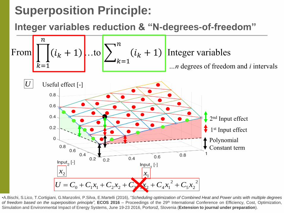
Superposition Principle:

Integer variables reduction & “N-degrees-of-freedom”

Useful effect [-]

1st Input effect

2nd Input effect

Polynomial

Constant term

2

25

2

1421322110 xCxCxxCxCxCCU +++++=

2x1x

U

𝑘=1

𝑛

𝑖𝑘 + 1 𝑘=1

𝑛

𝑖𝑘 + 1From

…n degrees of freedom and i intervals

…to Integer variables

•A.Bischi, S.Lico, T.Cortigiani, G.Manzolini, P.Silva, E.Martelli (2016), “Scheduling optimization of Combined Heat and Power units with multiple degrees

of freedom based on the superposition principle”, ECOS 2016 – Proceedings of the 29th International Conference on Efficiency, Cost, Optimization,

Simulation and Environmental Impact of Energy Systems, June 19-23 2016, Portorož, Slovenia (Extension to journal under preparation).

Superposition Principle:

Integer variables reduction

Eliminate the mixed term by linearly transforming the control variables!

𝑀 =𝑘11 𝑘12𝑘21 𝑘22

𝑥1𝑇 = 𝑘11𝑥1 + 𝑘12𝑥2𝑥2𝑇 = 𝑘21𝑥1 + 𝑘22𝑥2

𝑈 = 𝑐0 + 𝑐1𝑥1𝑇 + 𝑐2𝑥2𝑇 + 𝑐3𝑥1𝑇2 + 𝑐4𝑥2𝑇

2

𝑈 = 𝐶0 + 𝐶1𝑥1 + 𝐶2𝑥2 + 𝐶3𝑥1𝑥2 + 𝐶4𝑥12 + 𝐶5𝑥2

2

Q, Polynomial Quadratic Term Matrix:• Symmetric

• Diagonalizable to avoid mixed term

= 𝑥𝑇𝑄𝑥 + 𝑏𝑇𝑥 + 𝑐

By means of the orthogonal Q eigenvectors matrix M

•A.Bischi, S.Lico, T.Cortigiani, G.Manzolini, P.Silva, E.Martelli (2016), “Scheduling optimization of Combined Heat and Power units with multiple degrees

of freedom based on the superposition principle”, ECOS 2016 – Proceedings of the 29th International Conference on Efficiency, Cost, Optimization,

Simulation and Environmental Impact of Energy Systems, June 19-23 2016, Portorož, Slovenia (Extension to journal under preparation).


/ Commercial Stirling Engine – Laboratory

0

1

2

3840424446485052545658606264

N°

Bur

ners

[°C

]

Water circuit temperature

Tr Tm Tf N° BruciatoriAdditional NG consumption

Lower electricity output

m · cp · ( Thot – Tcold)

Thermal Power

G.Valenti, S. Campanari, P. Silva, A. Ravidà, E. Macchi, A. Bischi. “On-off cyclic testing of a micro-cogeneration Stirling

unit”, Energy Procedia (2015), pp. 1197-1201 DOI information: 10.1016/j.egypro.2015.07.152


/ Optimal Scheduling Impact

-2,00-1,000,001,002,003,004,005,00

He

at [

kWh

]

[Hour]

Cogenerated Dissipation Storage Charge Storage Discharge Demand Storage Levelb, 2)

-0,20

-0,10

0,00

0,10

0,20

0,30

Ele

ctri

c En

erg

y [k

Wh

]

[Hour]

Produced Purcheased Sold Demandb, 1)

-5,00

-4,00

-3,00

-2,00

-1,00

0,00

1,00

2,00

3,00

4,00

5,00

He

at [

kWh

]

Hour

Heat balance

Cogenerated Dissipation Storage Charge Storage Discharge Demand Storage Level

10 minutes time step




G.Valenti, S.Campanari, A.Bischi, P.Silva, A.Ravidà,

E.Macchi (2016), “Experimental and numerical

study of a micro-cogeneration Stirling unit under on-

off cycling operation”, under preparation.

Yearly problem & Performance-dependent parameters

Objective: minimization of Yearly Costs of Operation

=

=

=

=

-+++36524

1t

ttot,

36524

1t

ttot,on/off,

36524

1t

ttot,M,&O

36524

1t

,, ElCCC ttotF IncExEx -++

=

forf

36524

1t

th,

Hourly taxation on the electric

energy consumption (excise)

Monthly Threshold!

Periodic taxation on the electric

energy consumption (excise)

Monthly Threshold!

Periodic Incentives on the primary

energy savings (“white certificates”)

Yearly Bases!

«ad hoc» Rolling Horizon heuristic for the yearly schedule

Yearly constraints, e.g. Primary Energy Savings (PES) & first principle efficiency!

Extremely Challenging Mixed Integer Non-Linear Program (MINLP)

Due to Non-Linearity & High number of variables solving at once the whole problem

Rolling Horizon heuristic optimization method

Overall problem subdivided into a sequence of smaller (weekly) sub-problems:

Iteratively Optimize only the variables corresponding to a subproblem while fixing the

variables of all the other subproblems based on aggregated information

(Past weeks, already optimized weeks, future weeks based on typical weeks)

1 i… i+1 k-1 k+1k 52…

Future weeksPast weeks

Optimized weeks

Week k currently

being optimized

Weeks yet to be optimized

Resembled by «Typical Weeks»

Previously solved

Objective

Today, week i+1

A.Bischi, L.Taccari, E.Martelli, E.Amaldi, G.Manzolini, P.Silva, S.Campanari, E.Macchi. “A Rolling Horizon MILP Optimization Model for the

Scheduling of Tri-generation Systems with Incentives”. ECOS 2015 – Conference on Efficiency, Cost, Optimization, Simulation and

Environmental Impact of Energy Systems 30 June‐3 July 2015, Pau, France

Combined Heat and Power (CHP) plants,

Networks of CHP units feeding district heating

C.Elsido, A.Bischi, P.Silva, E.Martelli (2016), “Two-stage MINLP algorithm for the

optimal synthesis and design of networks of CHP units”, under revision (Energy).

Non linear effects of the size on the performance

The larger the size…

1) Lower fluid friction losses for isentropic efficiencies of machineries(Pumps, Compressors, Turbines)

2) Positive effects on specific costs (larger heat transfer areas, better materials and technologies)

• Steam Turbine

Isentropic efficiency of turbine stages from 60% till 92%

• Medium-small Gas Turbines plant (˂ 100 MWel): electric efficiency from 28,5% (5MW) till 41% (100 MW):

• Large Gas Turbines & Natural Gas Combined Cycles plants

Lower BUT Not-Negligible

• Gas-Fired Industrial Boilers

Thermal efficiency from 90% (1MW) till 93% (20MW)

Two stages optimization algorithmDecomposition Method

Higher Level (MINLP)DESIGN

OPTIMIZATION

𝒙𝐷 𝑜. 𝑓. (𝒙𝐷)

𝒙𝐷𝑂𝑃𝑇

Lower Level (MILP)SCHEDULING

OPTIMIZATION𝒙𝑆𝑂𝑃𝑇

1

2𝒙𝐷: design variables (unit

choice and size)

𝒙𝑆: scheduling variables

(on/off status, operativevariables and heat storagemanagement)

Metaheuristic,

e.g. genetic algorithm, particle

swarm, etc.

Units size

Units size



Typical Weeks decomposition

based on the optimization results!

Approximation error from 10 (standard typical Weeks) to 3%!

Reduce computational load by an accurate selection of typical periods,

e.g. Clustering techniques (K-means).

𝑤𝑎 =

𝑇𝑂𝐶0 − 𝑇𝑂𝐶𝑎𝑇𝑂𝐶0∆𝑥𝑎

1) Base Typical weeks determination via standard methods

2) Optimize the Total Operating Costs for the Base typical weeks (𝑇𝑂𝐶0)

3) Each input data variation ∆𝑥𝑎 ….keeping constant the others

4) For Each of the input variation optimize Total Operating Costs (𝑇𝑂𝐶𝑎)

5) Compute the weight (𝑤𝑎) for the input 𝑥𝑎

Weights calculation for input data (𝑥𝑎) like Thermal load, Electric load,

Temperature to reduce the approximation error

….for N design configurations



Achievements

➜ Development of an accurate MILP model for CCHP scheduling

Daily/Weekly basis ……………… heat storage

Validation ……………… Qualitative, Quantitative with Heuristic

➜ Extension up to Yearly Simulations

Iterative Simulations to Adjust Assumptions avoiding Non Linearity

Natural Gas / Electricity price according to monthly-yearly consumed volumes

Incentive calculation based on annual energy indexes, Primary Energy Savings

➜ Extension up to:

Higher number of degrees of freedom > 2,

by superposition principle & domain change for N variables (degrees of freedom)

Design, by two stage optimization algorithm,

➜ Future plans:

Load Forecast & Integration with Building physics model

Topology & Transport: Integration with Electric, Gas & Thermal grid

Stochastic & Robust optimization

Thank you for your attention.

[email protected]

PoliMI Colleagues:

E.Martelli, G.Manzolini, P.Silva, S.Campanari, E.Macchi

Group Energy COnversion Systems – GECOS, http://www.gecos.polimi.it/

PoliMI Students:

S.Lico, T. Cortigiani, C. Elsido, A. Emondi, G. Gentilini,

A.M. Castiglioni, D. Rossin, P. Colombo, E. Perez-Iribarren

Test Case – Energy Fluxes

QGT,PF,N,cog,HT

Qdiss,LT

FICEQICE,HT

FAB, LT

FAB,HT

QAB,LT

LH,stor

FGT

QICE,LT

Qdeg

QAB,HT

Heat Pump, compression

QHP,comp

Electric

Grid

EHP,comp

Epur

Qcust,HT

Qcust,LT

Esold

EGT

FGT,PF,N,cog

QGT,LT

QGT,HT

USer

ICE

Heat

Stor.

GT+PF

Aux. Boiler, LT

Ecust

EICE

Aux. Boiler, HT

Unit Performance* [kW] Input Electric Power Heat, HT Heat, LT

Gas Turbine

+ Post Firing

6765

+2500

2029 2380

+2350

944

Internal Combustion Engine 5198 2048 1483 988

Heat Pump, LT 280 1316

Auxiliary Boiler, HT 6818 6000

Auxiliary Boiler, LT 2666 2400

*Nominal Conditions, Temperature will change the units performance

Test Case – Units & Load Characterization

-6

-4

-2

0

2

4

6

8

10

0

1000

2000

3000

4000

5000

6000

7000

1 2 3 4 5 6 7 8 9 10 11 12 13 14 15 16 17 18 19 20 21 22 23 24

Am

bie

nt

Tem

pe

ratu

re [

°C]

Load

de

man

d [

kWh

]

Hours

HT heat

T amb

Electricity

LT heat

El.Cost

[€/kWh]

9th19th 8th;

20th23th

24th7th

Purchase 0,158 0,116 0,088

Sale 0,126 0,093 0,070

Fuel Cost [€/kWh] 0-24h

Prime Movers 0,06

Boilers 0,06

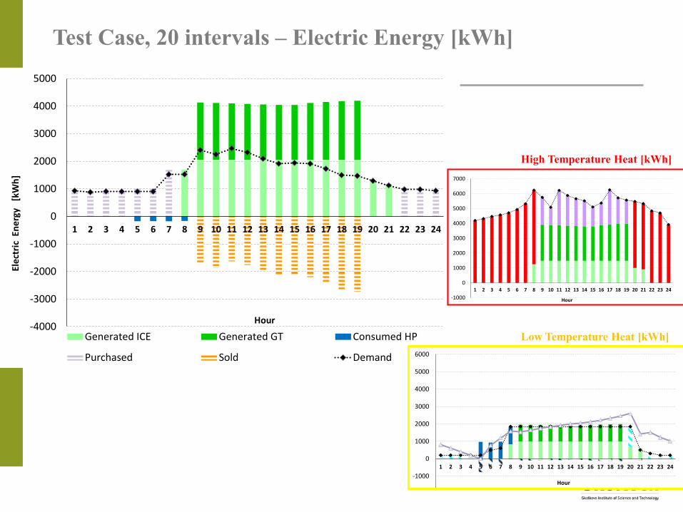
Test Case, 20 intervals – Electric Energy [kWh]

Low Temperature Heat [kWh]

High Temperature Heat [kWh]

-4000

-3000

-2000

-1000

0

1000

2000

3000

4000

5000

1 2 3 4 5 6 7 8 9 10 11 12 13 14 15 16 17 18 19 20 21 22 23 24

Ele

ctri

c E

ne

rgy

[kW

h]

Hour

Generated ICE Generated GT Consumed HP

Purchased Sold Demand

-1000

0

1000

2000

3000

4000

5000

6000

7000

1 2 3 4 5 6 7 8 9 10 11 12 13 14 15 16 17 18 19 20 21 22 23 24

Hig

h T

em

pe

ratu

re H

eat

[kW

h]

Hour

Cogenerated ICE Cogenerated GT GT Post Firing

Auxiliary Boiler Downgraded Demand

-2000

-1000

0

1000

2000

3000

4000

5000

6000

1 2 3 4 5 6 7 8 9 10 11 12 13 14 15 16 17 18 19 20 21 22 23 24

Low

Te

mp

era

ture

He

at [

kWh

]

Hour

Cogenerated ICE Cogenerated GT Heat Pump

Auxiliary Boiler Downgraded Storage Charge

Storage Discharge Dissipations Demand

Storage level, start

Test Case, 20 intervals – High Temperature Heat [kWh]

Low Temperature Heat [kWh]

Electric Energy [kWh]

-1000

0

1000

2000

3000

4000

5000

6000

7000

1 2 3 4 5 6 7 8 9 10 11 12 13 14 15 16 17 18 19 20 21 22 23 24

Hig

h T

em

pe

ratu

re H

eat

[kW

h]

Hour



-4000

-3000

-2000

-1000

0

1000

2000

3000

4000

5000

1 2 3 4 5 6 7 8 9 10 11 12 13 14 15 16 17 18 19 20 21 22 23 24

Ele

ctri

c E

ne

rgy

[kW

h]

Hour



-2000

-1000

0

1000

2000

3000

4000

5000

6000

1 2 3 4 5 6 7 8 9 10 11 12 13 14 15 16 17 18 19 20 21 22 23 24

Low

Te

mp

era

ture

He

at [

kWh

]

Hour





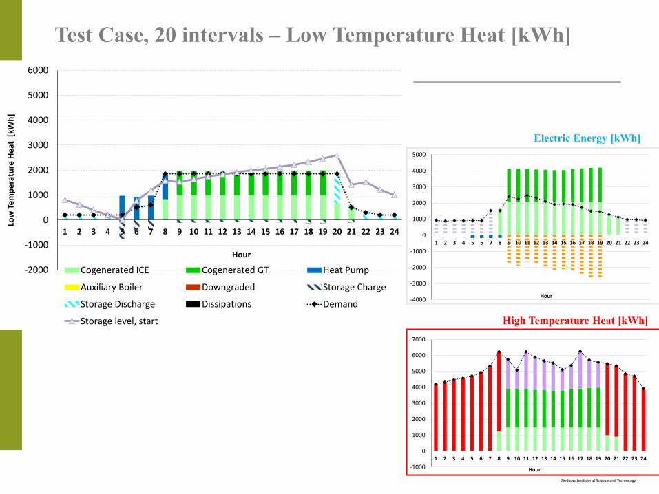
Test Case, 20 intervals – Low Temperature Heat [kWh]

Electric Energy [kWh]

High Temperature Heat [kWh]

-2000

-1000

0

1000

2000

3000

4000

5000

6000

1 2 3 4 5 6 7 8 9 10 11 12 13 14 15 16 17 18 19 20 21 22 23 24

Low

Te

mp

era

ture

He

at [

kWh

]

Hour





-4000

-3000

-2000

-1000

0

1000

2000

3000

4000

5000

1 2 3 4 5 6 7 8 9 10 11 12 13 14 15 16 17 18 19 20 21 22 23 24

Ele

ctri

c E

ne

rgy

[kW

h]

Hour



-1000

0

1000

2000

3000

4000

5000

6000

7000

1 2 3 4 5 6 7 8 9 10 11 12 13 14 15 16 17 18 19 20 21 22 23 24

Hig

h T

em

pe

ratu

re H

eat

[kW

h]

Hour



Results summary

Discretization Intervals► 5 intervals 10 intervals 20 intervals

Number of binary variables* 1944 6144 21744

Total number of variables 5712 13512 39912

Number of constraints 4685 8285 19085

Computational time (s) 22.69 68.28 293.86

Relative MILP gap (%) 9E-3 9E-3 9E-3

Objective function value (€) 14059.19 14055.43 14054.55

0,009% gap from the global optimum

corresponds to ~ 1,2€ out of 14060€ in

the worse case scenario

Excluding “macro mistakes”!!

*Without the «second-degree-of-freedom», post firing, the total number of

variables goes down to about 2400 (5 intervals) ÷ 6000 (20 intervals)!!

Short term differences, 20 intervals vs. 5 intervals

0,0

0,2

0,4

0,6

0,8

1,0

1,2

1 2 3 4 5 6 7 8 9 10 11 12 13 14 15 16 17 18 19 20 21 22 23 24 25

He

at P

um

p L

oad

s a

nd

Th

erm

al S

tora

ge [

-]

Hour

Heat Pump - 5 intervals Heat Pump - 20 intervals

Storage level, start - 5 intervals Storage level, start - 20 intervals

aldo bischi, ph.d. a.bischi@skoltech · associate characteristic curves to each unit, ... start-up)...

Documents