airline revenue management with callable products …
TRANSCRIPT

The Pennsylvania State University
The Graduate School
The Harold and Inge Marcus
Department of Industrial and Manufacturing Engineering
AIRLINE REVENUE MANAGEMENT WITH CALLABLE PRODUCTS
IN A MARKET OF SHRINKING MARGIN
A Thesis in
Industrial Engineering and Operations Research
by
2009 Sunwoo Hwang
Submitted in Partial Fulfillment
of the Requirements
for the Degree of
Master of Science
December 2009

The thesis of Sunwoo Hwang was reviewed and approved* by the following:
M. Jeya Chandra
Professor of Industrial Engineering
Thesis Advisor
Bing Li
Professor of Statistics
Paul Griffin
Professor of Industrial Engineering
Head of Harold and Inge Marcus Department of Industrial and Manufacturing
Engineering
*Signatures are on file in the Graduate School

iii
ABSTRACT
Since the Airline Deregulation Act was passed in 1978, revenue management (RM)
system has been markedly developed, and widely utilized by airlines. They could improve
their profit by maximizing revenue and minimizing cost based on the RM techniques.
RM approaches were adopted even in other industries where their usefulness was well
recognized. As a result, airline industry became more efficient, which caused diminished
arbitrage opportunities in the market. Moreover, the advent of information era enabled
customers to easily search and move to a lower-fare and higher-quality provider, using
internet access. In such a tightening market situation, shrinking margin forces the
management of airlines to take greater risk in order to increase their profits.
Several researchers recently introduced the concept of callable product, called a
promotional ticket in this thesis, that was risky but expected to increase profit. Called a
promotional ticket in this thesis, The callable product enables an airline to make money
by hedging potential spoilage and yield losses while satisfying customers‟ time-varying
demands. In this thesis, first the value of the risk premium is priced first, under
assumption that the product can be called at any time until expiration, which was not
addressed in previous works. Next, the expected profit increases through the
promotional ticket sales is examined. In addition, the matter of risk premium pricing
was facilitated by assuming that ticket price follows geometric Brownian motion. Also,
customer‟s demand is assumed to follow non-homogeneous Poisson process.

iv
TABLE OF CONTENTS
LIST OF FIGURES ........................................................................................................ v
LIST OF TABLES ........................................................................................................... vi
ACKNOWLEDGEMENTS ............................................................................................. vii
CHAPTER 1 INTRODUCTION AND MOTIVATION .................................................. 1
1.1 Revenue Management ...................................................................................... 1 1.2 Callable Products .............................................................................................. 2 1.3 Positioning and Outline .................................................................................... 4
CHAPTER 2 MODEL DEVELOPMENT ...................................................................... 7
2.1 Model Description ............................................................................................ 7 2.2 Model Assumptions ......................................................................................... 8 2.3 Notations .......................................................................................................... 9 2.4 Model Formulation .......................................................................................... 10
Objective Function .......................................................................................... 10 Constraints ...................................................................................................... 11
1) On the number of general tickets sold during each sales period t, , for all t = 1,2, …, T ......................................................................... 12
2) On the number of promotional tickets recalled during each sales period t, , for all t = 1,2, …, T ......................................................... 14
3) On the number of denied boarding during the last sales period, T ......................................................................................................... 16
CHAPTER 3 NUMERICAL RESULTS AND ANALYSIS ............................................. 19
3.1 Demand Model ................................................................................................. 19 Non-homogeneous Poisson Process .............................................................. 20 Parameter Determination............................................................................... 24
3.2 Ticket Price Model ........................................................................................... 25 Geometric Brownian Motion .......................................................................... 25 Parameter Determination............................................................................... 27 Risk Premium Valuation ................................................................................ 27
3.3 Optimization..................................................................................................... 29 Algorithm ........................................................................................................ 31 Numerical Example ........................................................................................ 32
3.4 Sensitivity and Scenario Analyses ................................................................... 35 Analysis on demand forecasts ........................................................................ 35

v
1) A case that high intensity of arrivals is expected in early periods. (mode = the 1st quartile, variance = 0.01) ....................................... 36
2) A case that moderate intensity of arrivals is expected in early periods. (mode = the 1st quartile, variance = 0.02) ......................... 38
3) A case that high intensity of arrivals is expected near the date of departure. (mode = the 3rd quartile, variance = 0.01) .................... 39
4) Market indifference due to flat arrival intensity (variance = 0.03) ............................................................................................................ 39
5) Profit rise caused by high correlation between demand and ticket price streams ........................................................................... 40
Analysis on ticket price forecasts ................................................................... 41 1) Effect of different expected markups ................................................ 43 2) Effect of projected volatilities ........................................................... 43
CHAPTER 4 CONCLUSION AND FUTURE WORKS ................................................. 44
4.1 Summary ........................................................................................................... 44 4.2 Future works .................................................................................................... 45 4.3 Conclusion ........................................................................................................ 47
REFERENCE ................................................................................................................. 49
Appendix A R code for the model optimization .......................................................... 52
vi
LIST OF FIGURES
Figure 3.1: Examples of Density function of the Gamma distribution with parameters , .............................................................................................................. 21
Figure 3.2: Examples of the density function of the Beta distribution with parameters , . ............................................................................................................ 23
Figure 3.3: Schematic flowchart of the proposed algorithm. .......................................... 30
Figure 3.4: Demand distribution as mode of the Beta distribution is 7 ........................ 38
Figure 3.5: Demand distributions as variance of the Beta distribution is fixed at 0.03 ................................................................................................................................. 40
Figure 4.1: Illustration of Low-price guarantee over time-varying price. ..................... 47
vii
LIST OF TABLES
Table 3.1: Summary of input parameters for promotional ticket sales. ........................ 32
Table 3.2: Parameters estimated by the forecasting department of XYZ Airlines. ...... 33
Table 3.3: Change in mode and variance. .......................................................................... 37
Table 3.4: Different scenarios in terms of changes in , . ............................................. 42

viii
ACKNOWLEDGEMENTS
I would like to express my gratitude to my research advisor, Dr. M. Jeya Chandra,
for his patience and guidance throughout my research for last two years. His constructive
advice and efforts to share his insight and wisdom have helped me to become a better
scholar and writer.
I also would like to thank Dr. Bing Li, a professor of Statistics, for his help and
advice that provided my research with rich solidity in mathematics and statistics.
In addition, I am grateful to Dr. Tom M. Cavalier, a professor of Industrial
Engineering, for his two-year teaching of operations research. I could make significant
academic improvement through his „beautiful‟ classes, and more significantly learn the
importance of basics. I also appreciate his recommendation that enabled my current
study at the KDI School.
My one and half year study abroad in the United States is indebted to my family.
Giving the greatest thank for their boundless love and devotion, I promise to return to
you with greater affection. Also I am deeply grateful to all PSUIEKSA members who
always treated me like their own brother. Wish all attain their desired ends and we
belong together for ages.
Beyond academic life, I could enjoy rich opportunities of learning through diverse
activities with my Penn State friends - Eve Ravelojaona, Qi Christine Liu, Nan Zhang,
Wan-ting Jenny Kuo, Veywel Cocaman, and Kasin Ransikarbum of the Industrial
Engineering department, and Corey Cochrane, Jan Visidal, and Ary Taha, the men of
White Course, and Armin Ataei. No matter where you are in the world, I will go find you
out. I love you all. So Long~.

ix
Lastly, I would like to thank to my friends in Korea as well, especially to ACES
members, for always having believed in and taken care of me who was used to be useless
at the bottom of the ladder. Without help of them, I could not likely have things that I
have now.
CHAPTER 1
INTRODUCTION AND MOTIVATION
In this chapter, a brief introduction of revenue management, which is the
foundation of this research, is given first, followed by an introduction of callable
products, mainly spotlighted in this work. In addition, relevant works that have been
conducted so far with respect to the callable products are introduced. The purpose and
contribution of this research are presented next.
1.1 Revenue Management
In 1972, Littlewood proposed his famous seat capacity control rule that discount
price bookings should be accepted as long as their revenue exceeds the expected revenue
of future high-fare bookings. The rule helped the start of revenue management research.
In 1978, Airline Deregulation Act was passed, removing any price restriction by airlines,
followed by a salient growth in revenue management techniques. Accordingly, profits of
airline companies remarkably increased (Fuchs, 1987). For instance, American Airlines
made an additional annual profit of more than 500 million dollars using revenue
management techniques (Smith et al. 1992). Its profit in 1997 exceeded one billion
dollars and it represented most of the company‟s revenues (Cook 1998).
The concept of revenue management is, however, not only applied to the airline
industry. It can be widely utilized in other industries having similar attributes, including
car rental, hotel, broadcasting, IT and internet service, railway, retailing, etc. The
common characteristics in revenue management practice are relatively fixed (inventory)

2
capacity, perishable inventory, price fluctuation, availability to sell products in advance,
ability to segment market, low marginal sales cost, and high marginal capacity change
cost (Kimes, 1989). The industries having limited capacity – tourism, transportation,
media, internet service providers, and entertainment – consistently face revenue
management problems. These industries want to maximize their total revenue, by
efficiently utilizing their restricted and perishable capacity. Revenue management
provides a theoretical and practical tool to resolve this sort of problems.
The revenue management problems are largely categorized into several different
areas such as pricing, overbooking, forecasting, and seat inventory control. Additional
issues include customer behavior analysis, performance measurement, and economics.
McGill and Van Ryzin (1999) provide a glossary of revenue management
terminology in their Appendix.
1.2 Callable Products
In the financial market, it is commonplace to see financial products being traded
with embedded options. Those options are issued in a rich variety of forms, depending
on the underlying assets such as stock, bond, interest rate, index, or currency, to name a
few. A callable bond has a unique attribute that allows the bond issuer to retain the right
of redeeming the bond at some time before the bond reaches its maturity. The presence
of a call option is advantageous to both the issuer and the bondholder. First, the issuer
can refinance his / her liability at a cheaper price by calling the bonds if interest rates go
down in the market, which results in higher current price, though the issuer pays a
higher coupon rate. Next, the investor or bondholder has the benefit of having a higher

3
coupon than with a straight (non-callable) bond. On the other hand, if interest rates fall,
the bonds get called and the investor can only reinvest at the lower rate.
The callable bond has two critical characteristics similar to the characteristics of
products of interest in the field of revenue management; both have maturity and both
their prices fluctuate as time goes by. Due to those similarities, several recently
published research papers, have tried to introduce the call property to the field of
revenue management in order to exploit the advantages of the callable bond.
Gallego (2004) initially proposed the notion and concept of callable products.
Under the assumption that low-fare customers arrive earlier, an airline sells both callable
product and non-callable product to the low-fare customers during the first selling
period. Customers who purchased the callable products would give an airline the right
(option) to recall the seat at a prescribed price at any time before the departure in the
future. The airline will notify the customer who bought the seat about the recall and pay
the recall price. The recall price will be higher than the low fare selling price and lower
than high fare selling price. Accordingly, airline will exercise the option only if it
concludes that high fare demands exceed available capacity (Gallego, 2004). For the
recalled seats, an airline will pay the recall price and resell them at higher fare.
The revenue management model of callable products of Gallego (2004) stems
from Biyalogorsky et al. (1999) and Biyalogorsky and Gerstner (2004). Biyalogorsky et al.
(1999) defined two potential losses of yield loss and spoilage loss which are trade-offs
that managers face when they quote a price. Yield loss implies selling a product at low-
price, losing an opportunity to sell it later at better price. Spoilage loss is the airline‟s loss
that occurs when it waits for high price sales, missing previous low price offer. Thus,
sellers will sell some of their products in advance in order to hedge the spoilage loss and
block some products against the yield loss to sell them later at higher price. Such a

4
hedging strategy, overselling with opportunistic cancellation, allows sellers more sales
than available capacity with a compensation for the customers who give up the products.
Gallego (2004) extended this concept of opportunistic cancellation to the „callable‟
product, which is consistent with the call provision of the callable bond in the financial
industry.
Such a callable product is not usually offered to customers in the airline industry .
Even so, some authors consistently claim that the new revenue management model that
contains the callable products would outperform earlier models in many aspects. After
Gallego (2004), Lee (2006) proposed an overbooking model of callable products based
on three-fare classes. Akgunduz et al. (2007) suggested a multiple-period, multiple-fare
model of the callable product and of the puttable product. Ravelojaona (2008) priced
the call and put option premium using financial option pricing theory – binomial option
pricing model, assuming that the ticket price movement follows a random walk.
1.3 Positioning and Outline
Akgunduz (2007) improved the two-period model of Gallego (2004) to the more
generalized multi-period model, under the assumption that the call option can be
exercised during the last period only. Ravelojaona (2008) also made this assumption
and defined the embedded options using European-style option framework; that is, the
airline which issued a callable product could not redeem it before the date of maturity.
Despite many significant contributions of those works, this assumption limits the most
distinct benefit of the callable products, which is an early redemption. In contrast, the
models of Biyalogorsky et al. (1999) and Gallego (2004) were free from this assumption,
since their models were basically of the two-period structure; sales during the first

5
period, followed by second period recall. As a result, this thesis proposes another multi-
period model that allows recall during any time period until maturity, so as to relax the
assumption and bring the concept of callable products closer to the reality.
Determining demand distribution and customers‟ arrival behavior is one of the
key issues in the field of revenue management, because of the uncertainty involved in
these. Recent papers have consistently insisted that the demand which follows non-
homogeneous Poisson process (NHPP) fits real demand well, and hence this thesis uses
NHPP to represent the customer‟s demand behavior. Even though Gallego (2004)
modeled the demand distribution using NHPP, its advantages were not indeed
spotlighted in his work, since the model was designed as a two-period one. On the other
hand, Akgunduz (2007) and Ravelojaona (2008) did not use a specific demand
distribution. They used self-constructed set of customers‟ arrival rate for each period.
One of the biggest uncertainties comes from change in ticket price. Empirical
investigations reveal that the ticket price tends to rise as time goes. In that sense,
lognormal process, widely known as geometric Brownian motion (GBM), seems to fit the
ticket price well. Accordingly, the ticket price movement in this thesis is assumed to
follow GBM. Meanwhile, Gallego (2004) and Akgunduz(2007) simply used likely sets of
ticket price for each fare class, while Ravelojaona (2008) assumed binomial movement
of ticket price, called a random walk. The binomial setting of the ticket price movement
facilitated valuating call- and put-option premiums.
A revenue management model is developed in Chapter 2 with an objective
function and necessary constraints. The step-by-step description of the model building
process will clarify the logic behind the model. Numerical results follow in Chapter 3.
Also, demand and ticket price models are built, and sensitivity analyses come next.

6
Chapter 4 summarizes the thesis, explicitly specifies not only the contributions but also
limitations of this work and makes suggestions for possible future extensions.

7
CHATPER 2
MODEL DEVELOPMENT
Callable ticket sales improve an airline‟s total expected profit from the single-flight,
single-fare and multiple-period profit model that is built in this chapter. In addition, a
callable ticket is called a promotional ticket and a non-callable ticket is called a general ticket
in order to help understanding how the designed model runs. Both terms are employed in all
the following chapters in this thesis.
2. 1. Model Description
An airline sells C tickets for one of its flights, which departs T periods later. Among
the C tickets, v tickets are promotional (callable) ones and sold only during the first period, t
= 1, while C-v general (non-callable) tickets are sold until the last period of flight departure,
that is until t = T. It is assumed that ticket price follows a Geometric Brownian motion which
shows an upward sloping trend. Promotional tickets have the following characteristics.
During the first selling period, the promotional tickets are sold at a price which is less than
general ones by an amount equal to the risk premium, . Then, the airline can recall the
outstanding tickets from the customers who purchased them at any time until the date of
departure, but at prescribed price higher than initial sales price, called recall price, R. It is
assumed that the airline wants to maximize its profit and hence, it would not recall
outstanding promotional tickets unless ticket price goes higher than the recall price R, since
otherwise the ticket sales generates negative revenue.
2.2. Model Assumptions
The assumptions made in this model are listed below.
(1) It is assumed that the promotional tickets are sold only during the first period of the ticket
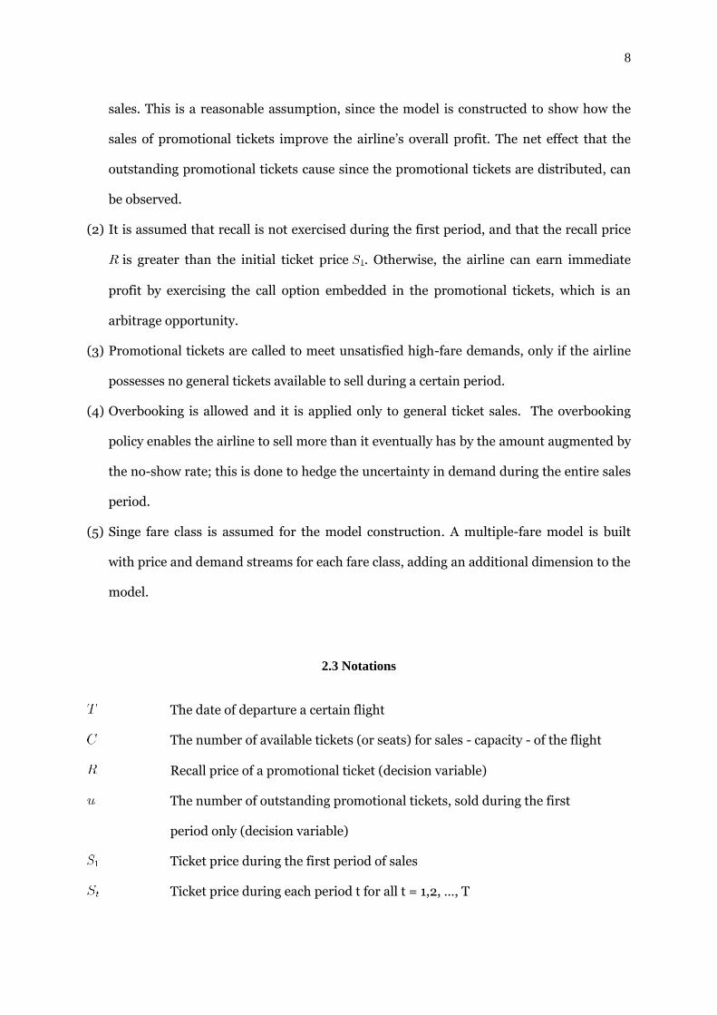
8
sales. This is a reasonable assumption, since the model is constructed to show how the
sales of promotional tickets improve the airline‟s overall profit. The net effect that the
outstanding promotional tickets cause since the promotional tickets are distributed, can
be observed.
(2) It is assumed that recall is not exercised during the first period, and that the recall price
is greater than the initial ticket price . Otherwise, the airline can earn immediate
profit by exercising the call option embedded in the promotional tickets, which is an
arbitrage opportunity.
(3) Promotional tickets are called to meet unsatisfied high-fare demands, only if the airline
possesses no general tickets available to sell during a certain period.
(4) Overbooking is allowed and it is applied only to general ticket sales. The overbooking
policy enables the airline to sell more than it eventually has by the amount augmented by
the no-show rate; this is done to hedge the uncertainty in demand during the entire sales
period.
(5) Singe fare class is assumed for the model construction. A multiple-fare model is built
with price and demand streams for each fare class, adding an additional dimension to the
model.
2.3 Notations
The date of departure a certain flight
The number of available tickets (or seats) for sales - capacity - of the flight
Recall price of a promotional ticket (decision variable)
The number of outstanding promotional tickets, sold during the first
period only (decision variable)
Ticket price during the first period of sales
Ticket price during each period t for all t = 1,2, …, T

9
Customer demands during the period t for all t = 1,2, …, T
The number of general tickets sold during the period t for all t = 1,2, …, T
The number of promotional tickets recalled and resold during the period t
for all t = 1,2, …, T.
Risk premium of the promotional ticket
Market interest rate
The probability of customers not showing up at the airport at the date of
departure T
The number of denied boardings
Unit cost of denied boardings
2.4 Model Formulation
In this section, the model is constructed ; an objective function is formulated first
followed by necessary constraints.
Objective Function
The objective of this research is to determine the optimal number of promotional
tickets, , that will be offered for sales and its recall price, , in order to maximize the
airline‟s expected profit. Four sources of revenue are considered. During the first period, an
airline earns money from sales of general tickets equal to , and from promotional
tickets sales that amounts to . The customers pay less for the promotional tickets
because they take callable risk embedded in the tickets. Thereafter, the airline makes money
from the sales of general tickets equal to . When there is
excess demand, the airline recalls corresponding number of outstanding promotional tickets
and earn an extra revenue equal to . But there is a cost

10
associated with this which is equal to . In addition, during the
very last period, the airline incurs a cost due to customers who show up and are denied
boarding, equal to . In summary, the expected profit, , is as follows:
=
; revenue that comes from promotional ticket sales during
the first period
+ ; revenue that comes from general ticket sales during the
first period
+
; revenue that comes from general ticket sales during the
remaining periods
+ ; revenue that comes from promotional tickets that are
called and immediately resold during the remaining
periods
-
; costs incurred from promotional tickets recalled during
the remaining periods
- ; cost incurred because of denied boarding on the date of
departure
In this, the two decision variables are– the number of promotional tickets sold during
the first period, , and the recall price, .
Constraints
The amount of ticket sold depends upon the expected customer demand and the
remaining capacity during each time period. The expected demand will be derived in the
following chapter. In this section, the number of the general tickets and promotional tickets
recalled to be sold during each time period and the number of denied boarding specified at
the date of departure will be derived, assuming that the expected demand is known.

11
1) The number of general tickets sold during sales period t, , for t = 1,2, …, T.
The total number of general tickets available for the entire sales periods depends
upon the seat capacity of a flight and the initial sales volume of the promotional tickets. The
seat capacity, which is equivalent to the number of tickets that the airline initially holds for
sale, is augmented by the no-show rate. The overbooking policy allows the airlines to
accommodate more ticket requests based on the no-show rate estimated from historical data.
Total number of general (non-callable) tickets
= total capacity on sales – total number of outstanding promotional (callable) tickets
= (2-1)
As the date of departure, T, approaches, the number of tickets held for sale steadily
decreases by an amount equal to the number of general tickets sold during each period. That
is, the right hand side of equation (2-1) less the number of outstanding general tickets
determines the number of general tickets available for sales during time period t, given in the
following.
The number of general tickets available for sale during period t
= total number of general tickets – the number of general tickets sold during the first
t-1 periods.
= (2-2)
The initial sales of the general tickets are easily determined from the minimum value
of the expected demand for general tickets during the first period and the total number of
general tickets available for the entire sales period. The initial general ticket sales is then
(2-3)
Likewise, the minimum value between the expected demand and the number of
general tickets available for sale during the period t, which is specified in (2-2), determines
the number of general tickets sold during period t, t = 2,3, …,T.

12
, (2-4)
In summary, the number of general tickets sold during each period is determined by
the expected demand while not exceeding available capacity augmented by the no-show rate.
2) The number of promotional tickets recalled during sales period t, , for t = 1,2, …, T.
Since it is assumed that general tickets are recalled before promotional tickets to
satisfy unsatisfied demand if an airline makes a recall request, outstanding promotional
tickets will be called only if the expected demand exceeds the number of general tickets
available for sale during a certain period of time. Hence, the unsatisfied demand during
period t is to be determined first, which is the positive difference between the expected
demand and the number of general tickets for sale during the period t.
Unsatisfied demand during period t
= expected demand – number of general tickets for sale during period t
=
if (2-5)
This is summarized as
Unsatisfied demand during the period t
= (2-6)
Next, in order to meet the unsatisfied demand during period t, the airline needs to
have enough capacity. The capacity, which is the remaining number of promotional tickets
during period t, is calculated as the difference between the total number of promotional
tickets and the number of promotional tickets sold until the previous period t-1.
Remaining number of promotional tickets on sale during period t

13
= total number of promotional tickets outstanding – number of promotional tickets
sold until period (t-1)
= (2-7)
Using (2-6) and (2-7), the number of promotional tickets to be called and
immediately resold during the period can be calculated, so as to meet the unsatisfied
demand. This is mathematically represented as follows.
Number of promotional tickets sold during the period t
= min (Unsatisfied demand during the period t, remaining number of promotional
tickets)
= (2-8)
However, the airline would never recall the promotional tickets unless the expected
ticket price during a certain period is less than the recall price . A binary variable
is introduced in equation (2-8) resulting in
,
(2-9)
, (2-10)
Equation (2-10) forces to have a value of either zero or one only. One additional
concern is that the promotional tickets will not be recalled during the first period, which is
taken care of in the assumption that the recall price is greater than the initial ticket price
.
14
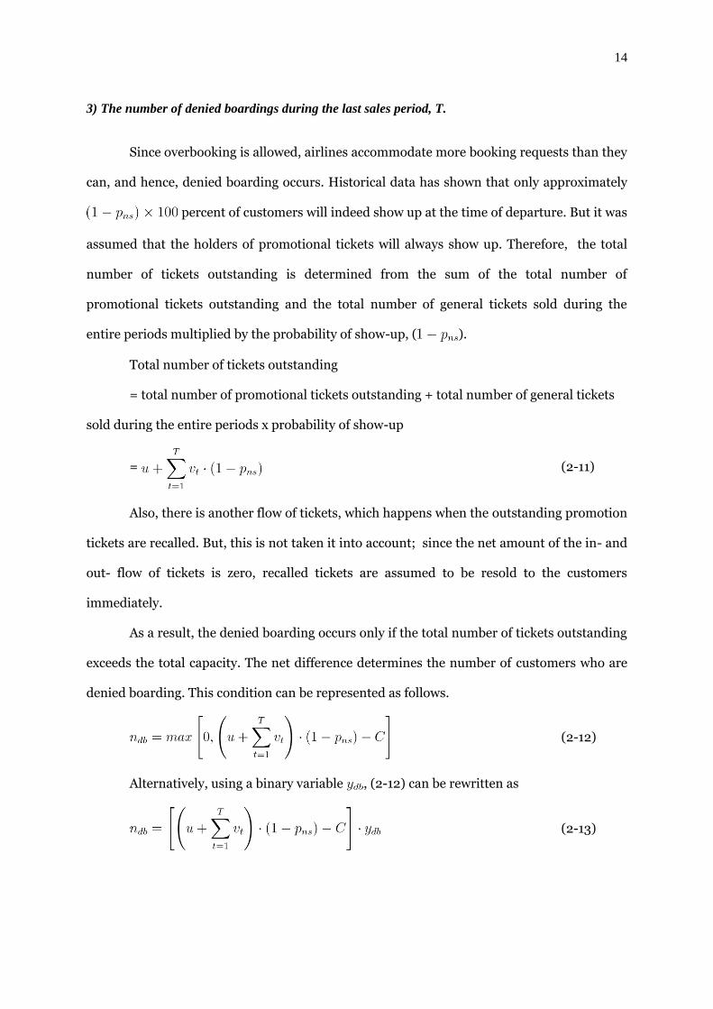
3) The number of denied boardings during the last sales period, T.
Since overbooking is allowed, airlines accommodate more booking requests than they
can, and hence, denied boarding occurs. Historical data has shown that only approximately
percent of customers will indeed show up at the time of departure. But it was
assumed that the holders of promotional tickets will always show up. Therefore, the total
number of tickets outstanding is determined from the sum of the total number of
promotional tickets outstanding and the total number of general tickets sold during the
entire periods multiplied by the probability of show-up, ( ).
Total number of tickets outstanding
= total number of promotional tickets outstanding + total number of general tickets
sold during the entire periods x probability of show-up
= (2-11)
Also, there is another flow of tickets, which happens when the outstanding promotion
tickets are recalled. But, this is not taken it into account; since the net amount of the in- and
out- flow of tickets is zero, recalled tickets are assumed to be resold to the customers
immediately.
As a result, the denied boarding occurs only if the total number of tickets outstanding
exceeds the total capacity. The net difference determines the number of customers who are
denied boarding. This condition can be represented as follows.
(2-12)
Alternatively, using a binary variable , (2-12) can be rewritten as
(2-13)

15
. (2-14)
CHAPTER 3
NUMERICAL RESULTS AND ANALYSIS
In chapter 2, a model was built that maximizes the expected profit by determining
both the optimal number of tickets to be sold and the optimal recall price of the promotional
tickets. But the performance of the model depends upon the accuracy of the forecast on
demand and price. Moreover, the selected ticket price model greatly affects how to price a
risk premium, which is one of the dominant factors in determining the model‟s performance.
For those reasons, it was assumed that ticket price follows a geometric Brownian motion
which appropriately fits actual ticket price movement and facilitates the risk premium
valuation as well.
With the values of the expected demand, ticket price and risk premium, the optimum
number of promotional tickets sale and recall price can now be determined, using the model
developed in Chapter 2. At the same time, is to be realized that the parameters that
characterize the demand and price are exposed to many different market variations. Hence,
the sensitivity of the expected profit to the change in parameters reflecting diverse market
situations will be examined now. Demand and price streams, generated using random
number generators instead of using the expected values, would help in studying the impact
of market uncertainty.

16
3.1 Demand Model
Demand model plays an important role in the models of the revenue management. In
this section, the demand model is defined and the expected demand of each period will be
derived. Then the estimation of parameters that characterize it will be described.
Non-homogeneous Poisson process
Non-homogeneous Poisson (NHPP) process is assumed for the demand model as it
has been known to be the closest model to the real demand pattern, in most recent works. In
this thesis, the NHPP with the following rate is assumed for the arrival process of ticket
demand.
(3-1)
where is a random variable that follows the Gamma distribution with a shape
parameter and a scale parameter , and is assumed to follow the standardized Beta
distribution over the interval with two shape parameters , . Although this rate
function was built mostly using empirical relevance, there is also a good theoretical reason,
for using Gamma distributed random variable, which is simple parameter estimation. The
density function of the gamma distribution is defined as
(3-2)
where
.

17
Several Gamma distributions are exhibited in Figure 3.1 with different sets of
parameters ( , ). The expected value and standard deviation of the Gamma distribution are
as follows.
(3-3)
(3-4)
Figure 3.1 displays distributions with the same expected value but different standard
deviations. For instance, the solid curve with parameters (4, 75) in the figure has a mean of
300 and a standard deviation of 150. The density function of the Beta distribution with
parameters and , is defined over the interval as
(3-5)
Figure 3.1: Examples of Density function of the Gamma distribution with parameters ,

18
in which is the Beta function
1
Figure 3.2 depicts three sample curves of the Beta density function with respect to
three different parameter sets of ( , ). All of them have the same mode of 21 over the
interval of [1, 28] but different variances which determine arrival intensity. The way the
parameters are estimated in terms of the known mode and variance will be discussed in
detail later.
Now using the formula (3-3) and (3-5), a formula can be derived which yields the
expected demand of each time period. The expected value of demand (ticket purchase
requests), which is Poisson distributed with the rate during period , is specified by
. (3-6)
Figure 3.2: Examples of the density function of the Beta distribution with parameters ,

19
where
To conclude, a non-homogeneous Poisson process is characterized by its rate
function , which represents arrival intensity. Defined in the formula (3-1), the rate function
was introduced by Bertsimas and de Boer (2005), which follows Weatherford et al. (1993).
The Beta distribution is often used to model events that are constrained to take place within
an interval defined with minimum and maximum values and modeling the arrival intensity
by using the beta distribution allows to exhibit a wide range of unimodal arrival patterns;
the higher for any time period , the more arrivals are expected to come. In addition, the
random variable adds an extra level of randomness to the non-homogeneous Poisson
process. That is, using the Beta distribution function in the formula (3-4), total demand
represented by the random variable is distributed over the time interval .
Parameter Determination
In order to generate the expected customers‟ demand, proper parameter estimation
has to come first. The parameters , of the Gamma distribution are easily specified by
defining the mean and standard deviation of using the formulas (3-3) and (3-4). Here,
illustrates an expected total demand of air tickets during the whole period of ticket sales.
For instance, suppose that there is an airplane that have 300 available tickets (seats) for
sales. If we assume that the expected value of the total demand is 400 and its standard
deviation is 200, that is
, ,
then the parameters satisfying both equations together become = 4 and = 100,
respectively. Likewise, the parameters , of the beta distribution function are determined
by specifying a mode and a variance of the beta distribution such that

20
(3-7)
(3-8)
Suppose that for instance that an airline company sells air tickets from January 1st to
December 31st, the date of departure and expects the ticket purchase requests will be the
highest during September. Then, we can simply set the mode of the Beta distribution as 270
over the interval [1,360]. If we assume, in addition, that the variance of the Beta distribution
is 1%, that is
,
then we can specify the value of parameters , which satisfies both equations together.
They are = 10 and = 4, respectively.
3.2 Ticket Price Model
An airline company prices its tickets strategically based on the expected demand. It is
an usual practice that the airline sells tickets at cheaper price in the early periods of its sales
in order to draw relatively small amount of demand and accommodate high fare demands
later near departure. This prevents yield loss and spoilage loss defined in Section 1.1 and
enhances profit of the airline. This thesis defines a proper price model of the geometric
Brownian motion that an airline‟s ticket price can follow. Next, the manner that its
parameters are specified is illustrated and a risk premium is priced based on the model.

21
Geometric Brownian Motion
It is assumed that the ticket price follows geometric Brownian motion. It seems
logical, because the actual ticket price tends to increase over time, but with short-term
fluctuation. Given initial ticket price , discrete-time ticket price model is then defined as
(3-9)
for time period , , where is a mean drift and is volatility. The
variable, , is a random number that follows a standard Normal distribution and the time
step, dividing the whole time period into T intervals, is specified as . This model
simply becomes
,
(3-10)
which implies that the ticket price, , for each period can be simply computed with
the initial sales price multiplied by t-1 ; that is,
, for all , .
(3-11)
Then, the expected value of during the time period is
2
(3-12)
for each time period , . Therefore, the expected value of the ticket prices
for each period can be calculated in a closed form, as derived in the formula (3-12).

22
Parameter Determination
It can be seen that the parameter estimation problem is also simplified; the mean
drift over a predetermined time interval is to be estimated, which represents the rate
of increase in ticket price between the dates of ticket sales and of departure. For instance, if it
is assumed that a ticket, for a trip from New York to Paris 3 months from now, costs $200
today but its price is expected to rise by 25% for next three months, then the mean drift
= .25.
Risk Premium Valuation
Promotional tickets, mainly spotlighted in this thesis, include call provision as
defined in Chapter 1 and hence the value of the provision can be measured using financial
option theory. Unlike European-style call option, however, the moment of the option
exercise of the promotional tickets is not restricted to the date of maturity; that is, it can be
categorized as American-style call options, which allows an exercise at any time before a
prescribed expiry date. The early exercise feature of this option complicates the valuation
process since the standard Black-Scholes model cannot be used. In this paper, an alternative
approach is adopted; each period of the ticket sales process is considered as a maturity of
European call option and have the prices of each option that expires at the end of each
period is multiplied by the density function of the Beta distribution standardized on the
interval . This calculation provides the model with a sort of weighted-average value of
the call option, which is price of the risk premium of the promotional ticket purchase.
The value of the European-style call option during the time period t is calculated
using the following formula (3-13) (p.80, Higham, 2004).
(3-13)
where represents the standard Normal distribution function.

23
Using the formula (3-13), the present values of European-style call options which
mature each period can be calculated, simply by replacing by and by , respectively.
Then the formula becomes
(3-14)
where
In order to price American-style option through a sort of “weighted-averaging” way
using European-style option values, it is of mighty importance to allot proper weights for
each period. As referred earlier, one of the most critical factors when a firm makes a pricing
decision is the expected demand. Hence, it appears natural to employ the Beta distribution
function in the formula (3-4), which has been used to determine arrival intensity of each
period in the demand model, as weights in pricing the risk premiums of promotional tickets.
Specifically, the formula (3-14) can be multiplied by in the formula (3-4) having the same
values of parameters with the demand model. It should be noted however that this
multiplication should be done only if , because otherwise the call exercise will result
in a negative profit to the airline company.
3.3 Optimization
In sections 3.1 and 3.2, the demand and ticket price models were developed with
properly estimated parameters. Using the models in the formulas (3-6) and (3-12), the

24
expected values and of both models can be obtained. Accordingly, all the
ingredients, that are needed to optimize the model developed in Chapter 2, are available. As
defined in Chapter 2, the objective of this thesis is to determine the optimal number of
promotional tickets, , that will be offered for sale and its recall price, , in order to
maximize the airline‟s expected profit. To find the optimal values of and , cyclical
coordinate search method, which is a relatively simple method, is employed. This chapter
illustrates the algorithm of the search method with a flow chart in Figure 3.3, and presents a
numerical example with given set of parameters so as to evaluate the performance of the
model.

Figure 3.3: Schematic flowchart of the proposed algorithm

26
Algorithm
First, the input parameters: need to be specified. Then,
with the specified values and estimated using the formulas
(3-6), (3-7), and (3-8), need to be calculated . Also, can be calculated based on the
projected parameters of as described in Section 3.2, . Now to conduct
the cyclical coordinate search, increments along each direction and an arbitrary
small number of and the initial value of that satisfies , , need to
be chosen.
The main problem is as follows. First, find the value of needs to be found, that
maximizes expected profit by increasing or decreasing by the amount of ;
subsequently move should be moved as much as ; that is, .
Second, the value of needs to be found, that maximizes the expected profit by
increasing or decreasing by the amount of ; subsequently should be moved as
much as ; that is, . It should be noted that the risk premium, ,
has to be recalculated whenever the recall price, , has different value, since is
dependent on . Hence, it is natural to have altered along with a change in .
Consequently, this process needs to be stopped, if the difference between the old and
new sets of and is less than predetermined value of . Otherwise, the process of
finding profit-maximizing and needs to be repeated, having new sets of values of
and as the new starting point.
The entire process is schematically illustrated in Figure 3.3, and the code written
is given in Appendix A. Use of this algorithm allows comparison of profits between the

27
case of offering and not offering promotional tickets, which also reveals how good the
model is.
Numerical Example
An algorithm that optimizes the expected profit is described in this section. This
numerical example describes the algorithm and finds an unique solution of the given
problem.
Suppose that there is an airline company called XYZ Airlines, and one of its
flights which departs from Boston to Tokyo thirty days from now, has 300 seats available
for sale. To enhance sales profit, the management of XYZ Airlines decides to sell
promotional tickets that have several distinct features 2 days later for a duration of one
day; these tickets are offered at cheaper price than the general ones. But, buyers have to
assume a risk that tickets can be recalled at a certain price, suggested by the airline
before purchase. The airlines wants to figure out the number of promotional tickets to
offer for sale, , and its recall price, , that maximizes the expected profit while
encouraging customers to buy the tickets, even with the perceived risk. Additional
information necessary to solve this problem is as follows. The price of general rickets
(non-promotional tickets) two days later will be $600. No-show rate estimated from
historical data is 30%. Denied boarding cost incurred due to overbooking as much as the
no-show rate is $200 per ticket. Prevailing monthly interest rate in the market is 4%;
that is 0.2% daily. A summary of the input parameters are given in Table 3.1.

28
The airlines also has its own forecasting division. It expected that the total
demand would be as much as the number of holding tickets, , and it is assumed to
follow a Gamma distribution with a standard deviation of 150. Moreover, the division
concluded that the demand would reach its peak a week before the date of departure,
exhibiting the highest arrival intensity. The Beta-distributed arrival intensity is
generated with a known variance of 0.01. On the other hand, ticket price is anticipated to
rise by 30% during the interval between promotional ticket sales and flight departure,
considering this market demand as well as diverse market factors. Subsequently, the
values of indispensable parameters to solve this problem is estimated based on the
forecasts, which is summarized in Table 3.2.
Table 3.1: Summary of input parameters for promotional ticket sales
Input parameters Value
28
300
$600
0.2%
30%
$200

29
Forecasts
Parameters
Estimation
Total Demand
= 300 = 2.04
= 150 = 147
Arrival Intensity Mode = 21 = 13.7
Variance = 0.01 = 5.2
Ticket Price Change Markup = 30% = 0.3
= 0.3
The problem of XYZ Airline results in the following output by using the model
built in Chapter 2 and the algorithm addressed in this section.
= 90 tickets,
= $ 689,
= $ 76.8,
= $ 261334.5,
= $ 212798.0,
improvement = 22.8%
It appears to be optimal from this output data to sell 90 promotional tickets with
a stated recall price of $689. At the same time, the price of a promotional ticket turns out
to be $523.2 as the risk premium of the promotional ticket purchase is priced as $76.8;
= $600 - $76.8 = $523.2, from the model proposed in Chapter 2. In other words,
the airline is expected to sell 90 promotional tickets for its flight from Boston to Tokyo
Table 3.2: Parameters estimated by the forecasting department of XYZ Airlines
30
when it offered the ticket at $523.2 with the recall price of $689. This expected ticket
sales would result in a maximized profit of $261,334.5, which gives an improved profit
of 22.8%, compared to the sales of only general tickets; the airline anticipates to earn
$212,798.0 when it sells all of its 300 tickets as the general price.
From this numerical example, it can be seen that that the promotional (callable)
ticket sales combined with general (non-callable) ones contribute to increasing an
airline‟s expected profit. Of course, there might be other factors that need to be included
in the model. We conduct sensitivity analysis in the next section in order to measure the
model‟s performance under diverse market conditions.
3.4 Sensitivity and Scenario Analyses
In this section, the sensitivity of several parameters reflecting market conditions is
studied.
Analysis on demand forecasts
Demand for ticket sales is known to be larger as the date of departure approaches.
However, the opposite trend can also be observed in the market from time to time. For
the reason, the quartiles of the interval to indicate different modes are set, which
represent customers‟ arrival intensity. This treatment is equivalent to setting each mode
to mark .25, .50, and .75 spots on a given interval in order to represent skewness of the
arrival intensity.

31
1) A case that high intensity of arrivals is expected in early periods. (mode = the 1st quartile,
variance = 0.01)
Figure 3.3 illustrates the cases of early concentration of arrivals, which
corresponds to the first three scenarios described in Table 3.3. In such cases, an airline
would better sell its promotional tickets at a cheaper recall price. It is because the price
of risk premium, affected by the arrival intensity, is being priced lower under the
assumption that the ticket price goes upward as time goes by. Thereby, the probability of
recall is set high around the low-fare class and it will drag the recall price down. Table
3.3 provides numerical explanation of this argument. In scenario I, which is related to
mode = 7 and variance = 0.01, selling promotional tickets at $556.3 with recall price of
$619, turns out to be optimal; the mode of 7 implies high concentration of arrival
intensity in between the first and second quarters. As compared to the other scenarios,
this result reveals the same result. The risk premium of $43.7 is the lowest among all
scenarios and hence the highest recall price is anticipated though it was indeed not. The
recall price of $619 is the largest among the first scenarios that have the same mode, but
it is lower than in other scenarios having greater modes, due to the highest early recall
probability.

Table 3.3: Change in mode and variance
Scenarios Total demand
mode variance
I 7 0.01 5.2 13.7 98 $619 $43.7 $241,236 $190,815 26.4%
II 7 0.02 2.1 4.3 93 $606 $69.2 $241,390 $193,106 25.0%
III 7 0.03 1.4 2.3 95 $606 $83.0 $242,574 $194,200 24.9%
IV 14 0.01 12.0 12.0 93 $653 $56.4 $251,066 $201,507 24.6%
V 14 0.02 3.7 3.7 92 $626 $84.4 $248,515 $201,625 23.3%
VI 14 0.03 1.6 1.6 92 $606 $106.8 $246,975 $200,762 23.0%
VII 21 0.01 13.7 5.2 90 $689 $76.8 $261,335 $212,798 22.8%
VIII 21 0.02 4.3 2.1 91 $646 $106.1 $256,067 $209,833 22.0%
IX 21 0.03 2.3 1.4 93 $619 $120.3 $252,365 $205,648 22.7%
(* with fixed = 4, = 75 and = 0.3, = 0.3)

2) A case that moderate intensity of arrivals is expected in early periods. (mode = the 1st
quartile, variance = 0.02)
The scenario II in Table 3.3 which has the same mode 7 but has different variance
0.02, exhibits an increased risk premium and decreased recall price compared to
scenario I. This is subject to call risk of promotional tickets, distributed more widely over
low- and high-fare classes. Under such a forecast of market condition, an airline would
offer promotional tickets at cheaper price, pursuing its right to exercise recall tickets at a
lower price. This scenario II is depicted in Figure 3.4 with a dashed line.
Figure 3.4: Demand distribution as mode of the Beta distribution is 7
34
3) A case that high intensity of arrivals is expected near the date of departure. (mode = the 3rd
quartile, variance = 0.01)
The last three scenarios with modes set between 3rd and 4th quarters, provides
similar comparison with those between 1st and 2nd quarters. The greater variance in
arrival intensity, the higher risk premium and the lower risk price is required. Compared
to other scenarios with lower modes, however, both the risk premium and recall price are
more costly due to high concentration of demand around high-fare classes. Subsequently,
low sales of tickets would be better and it turned out to be true as illustrated in Table 3.3.
For instance, scenario VII reveals that the risk premium of $76.8 is the highest among
scenarios having the same variance, and recall price, reflecting the high risk in premium
as well as intensive demand around the mode, is also the highest.
4) Market indifference due to flat arrival intensity (variance = 0.03)
Scenarios III, VI, and IX with the highest variance of 0.03, exhibit the values in
each category that have closer values. In Table 3.3, the gap between values of different
modes is reduced as variance increases, and values associated with modes equal to 7 and
to 21 converge to the values with the mode of 14. For example, when the variance is equal
to 0.01, the numbers of promotional tickets to be soldl are 98, 93, 90 for each mode. But
when the variance is equal to 0.03, they are 95, 92, 93 for each mode as shown in the
table. The gaps between the recall prices also exhibits the same results; they are $619,
$653, and $689 for the modes associated with a variance of 0.01, but are $606, $606,
and $619 when the variance is equal to 0.03. If variances are further increased, the
values will come closer. This is because greater variance results in relatively flat
distribution in customers‟ arrival, as depicted in Figure 3.5. The figure illustrates

35
demand distributions for scenarios III, VI, and IX which have the same variances but
different modes. It should be noted that the solid curve with = 1.4 and = 2.3 in
Figure 3.5 is identical with the dotted curve in Figure 3.4. The flatted curve shapes look
alike in spite of different modes. Therefore, it can be concluded that the demand would
be less affected by the arrival intensity when higher variance is expected in the market.
5) Profit rise caused by high correlation between demand and ticket price streams.
It can be observed in Table 3.3 that the expected profit increases along with
bigger modes regardless of promotional ticket sales. This seems natural since customer
arrivals get concentrated around high-fare classes with respect to greater modes. For
Figure 3.5: Demand distributions as variance of the Beta distribution is fixed at 0.03

36
instance, expected profits as promotional tickets are not offered consistently increase
from $190,815 with mode = 7 to $201,507 with mode = 14 and $212,798 with mode = 21.
This also holds true for promotional tickets being offered; the expected profits, , are
$241,236, $251,066, $261,335 for the modes in the ascending order. Since ticket price is
assumed to rise over time, higher mode also implies greater correlation between demand
and ticket price and it can be said that the overall profit would be greater if the
correlation between demand and ticket price is higher.
Analysis on ticket price forecasts
In this section, the sensitivity of the expected profits with respect to a mean drift,
, and a volatility, is analyzed, which characterizes ticket price movement. It should be
noted that the set of ticket price markups employed for the analysis ranges between 15%
and 30%. The high price markup was assumed to reveal distinct differences in expected
profits due to change in values of , .

Table 3.4: Different scenarios in terms of changes in ,
Scenario
s
Ticket price change
Markup
I 15% 0.15 0.15 40 $643 $48.4 $246,846 $224,011 10.2%
II 0.25 40 $646 $55.3 $246,507 $224,011 10.0%
III 0.35 40 $653 $115.1 $243,976 $224,011 8.9%
IV 20% 0.20 0.15 40 $658 $57.3 $254,593 $231,828 9.8%
V 0.25 40 $658 $58.1 $254,561 $231,828 9.8%
VI 0.35 40 $662 $76.5 $253,746 $231,828 9.5%
VII 25% 0.25 0.15 40 $673 $67.1 $262,597 $239,910 9.5%
VIII 0.25 40 $673 $67.1 $262,595 $239,910 9.5%
IX 0.35 40 $673 $72.0 $262,402 $239,910 9.4%
X 30% 0.30 0.15 40 $681 $83.9 $270,758 $248,264 9.1%
XI 0.25 40 $681 $83.9 $270,758 $248,264 9.1%
XII 0.35 40 $681 $84.7 $270,727 $248,264 9.0%

1) Effect of different expected markups
Compared with others having identical volatilities, both the risk premium and
recall price can be seen to grow coincidentally as increases. Markup in risk premium
implies cut in price of the promotional ticket. Because market price of air tickets is
anticipated to increase as much as the markup amount, greater price cut and higher
recall price must be offered to sell the same amount of promotional tickets. In fact,
scenarios I, IV, VII, and X exhibit constant increase in price of recall and risk premium,
which can be interpreted as cost which an airline has to incur. However, the increased
costs are compensated with the augmented expected profit for airlines who calls
outstanding promotional tickets and resells them at higher market price.
2) Effect of projected volatilities
Compared with others having identical mean drifts, we see both risk premium
and recall price increase simultaneously as volatility augments. This is the same result as
we change with fixed volatility, , but because of the different cause. It was because
customers had to bear greater risk due to increased market uncertainty. The change in
price of risk premium and recall price are observed in Table 3.4. However, the changes
solely means increase in cost which results in decrease in expected profits. We can see
from scenario I, II, and III that expected profits are decreasing along with increases in
risk premium and recall price.

39
CHAPTER 4
CONCLUSION AND FUTURE WORKS
4.1 Summary
Many research topics that have been addressed in recent years in the field of
revenue management; relatively new among them is an application of call feature, which
is can be applied to the sale of an airline. Iin 1999, Biyalogorsky et al. introduced a
conceptual framework of the callable product, though the term “callable product” was
not yet introduced then. They defined two potential losses anticipated due to time-
varying ticket price markup and attempted to hedge them by offering callable products.
Based upon their work, Gallego established a theoretical framework of the callable
product and introduced the term “callable product” in his working paper in 2004
Basically, the concept of the callable product was proposed in order to foster early
tickets purchase while meeting high-fare demands that come later within the time
horizon of ticket sales. Its call property benefits both the airlines and customers. Since
ticket price is assumed to rise as time goes by, if an airline offers further discount on its
tickets in early periods, then consumers would enjoy deeper price cut. At the same time,
an airline could avoid spoilage loss caused by retaining tickets. Yet, an airline may suffer
yield loss, since, if customers who concern much about future price markup purchase a
majority of tickets, it would fail to satisfy high-fare demands. Therefore, if an airline has
the option of calling and reselling outstanding tickets later to meet the high-fare
demands, its profit would increase significantly. Besides, customers might be able to
enjoy a portion of the margin generated by the high-fare sales if the compensation
offered for recall of tickets is high enough. In sum, the callable product sales enables

40
both an airline and a customer to enjoy advantages and to prevent anticipated loss
simultaneously.
In 2007, Akgunduz put this callable product concept a multiple-period and
multiple-fare class framework. Using this framework, Ravelojona find the optimal value
of the call option tickets using binomial option pricing model, which is one of the
prevailing financial option valuation techniques. But the option, which can be looked
upon as an European-style one, has limited its use as it allows recall of the tickets only
during the late period. In this thesis, the restriction is relaxed; outstanding promotional
tickets are callable at any moment until departure. In addition, non-homogeneous
Poisson process, known to be the closest to the real demand distribution in recent works,
is chosen to specify demand model and geometric Brownian motion is chosen to fit ticket
price movement. This is also reasonable since actual ticket price tends to rise upwards
over time. These treatments are expected to improve reliability of the model.
4.2 Future works
Several further researches would improve usefulness of the model developed in
this thesis. First of all, ticket price is assumed to follow geometric Brownian motion and
hence risk premium of the promotional ticket was priced using applied Black-Scholes
model. Unlike European-style options which are priced through standard Black-Scholes
model, however, the risk premium that can be modeled as an American-style call option
can be used in the model. The optimum value of the risk premium can be obtained.
The model in this thesis employed expected values of demand and ticket price to
model expected profit, which subsequently facilitates solving an optimization problem.
In order to reflect the model‟s complexity and market uncertainty, however, it would be

41
also meaningful to find the optimal solution using simulation optimization; that is, one
could generate random demand and price streams using a random number generator
based on sophisticatedly estimated parameters and then use the random streams instead
of expected values.
Other minor extensions include industry-specific customization of the model.
Since the revenue management techniques are widely utilized in various industries,
which sells so-called perishable products, customized models would increase
applicability toward certain industries.
Lastly, it is recommended to use the concept of low-price guarantee, which is a
popularly issued topic in marketing, into a revenue management modeling, since the
concept of callable products was initially proposed in the field of marketing by
Biyalgorski et al. in 1999. The low-price guarantee is usually categorized as market-based,
competitor-based, or self-based pricing strategies. Among them, a self-based low-price
guarantee could be combined with the revenue management model. With the guarantee,
an airline can offer a price cut if price goes below initial sales price of the promotional
tickets. Such an additional cost against an airline, however, would promote ticket sales
by providing the additional benefit to customers. Moreover, the payout for customers
can be easily priced, considering the payout as a lookback option, under the assumption
that the ticket price follows geometric Brownian motion.
Figure 4.1 exhibits the pricing strategy , where denotes the actual lowest price
observed in the market during the time period t. Then, the payout to the customers is

42
After all, each customer enjoys a total revenue of if an airline calls
outstanding promotional tickets, since recall price is set above . At the same time, an
airline enjoys a margin above the recall price, , that is, , by reselling the tickets
recalled.
Figure 4.1: Illustration of Low-price guarantee over time-varying price

REFERENCES
ANDERSON, C., H. RASMUSSEN, M. DAVISON. 2004. REVENUE MANAGEMENT: A REAL OPTIONS
APPROACH. NAVAL RES. LOGISIT. 51(5) 686-703.
BERTSIMAS, D., I. POPESCU. 2003. REVENUE MANAGEMENT IN A DYNAMIC NETWORK
ENVIRONMENT. TRANSPORTATION SCIENCE. 37(3) 257-277.
BLAIR, M. 2002. DYNAMIC PRICING: THE NEW DIVERSITY OF REVENUE MANAGEMENT.
INFORMS TRIENNIAL MEETING. EDINBURGH, SCOTLAND.
CARROLL, W., R. GRIMES. 1995. EVOLUTIONARY CHANGES IN PRODUCT MANAGEMENT:
EXPERIENCES IN THE CAR RENTAL INDUSTRY. INTERFACES 25(5) 84-104.
CONZE, A., R. VISWANATHAN. 1991. PATH DEPENDENT OPTIONS: THE CASE OF LOOKBACK
OPTIONS. J FINANCE 46(5) 1893-1907.
COOK, T. 1998. SABRE SOARS. ORMS TODAY 25(3) 27-31.
CROSS, R. 1995. AN INTRODUCTION TO REVENUE MANAGEMENT. HANDBOOK OF AIRLINE
ECONOMICS. D. JENKINS, C. RAY, EDS. MCGRAW-HILL, NEW YORK, 443-458
CVITANIC, J., F. ZAPATERO. 2004. INTRODUCTION TO THE ECONOMICS AND MATHEMATICS OF
FINANCIAL MARKETS. MIT PRESS, CAMBRIDGE, MA.
DAN C. I., L. A. GARROW. 2008. A HAZARD MODEL OF US AIRLINE PASSENGERS’ REFUND AND
EXCHANGE BEHAVIOR.
DIXIT, A. K., R. S. PINDYCK. 1994. INVESTMENT UNDER UNCERTAINTY. PRINCETON UNIVERSITY
PRESS, PRINCETON, NJ.
DUFFIE, D. 2001. DYNAMIC ASSET PRICING THEORY. PRINCETON UNIVERSITY PRESS,
PRINCETON, NJ.
FUCHS, S. 1987. MANAGING THE SEAT AUCTION. AIRLINE BUS. 7 40-44.

44
GERAGHTY, M. K., E. JOHNSON. 1997. REVENUE MANAGEMENT SAVES NATIONAL CAR RENTAL.
INTERFACES. 27(1) 107-127.
GOLDMAN, M., H. SOSIN, M. GATTO. 1979. PATH DEPENDENT OPTIONS: BUY AT THE LOW, SELL
AT THE HIGH. J. FINANCE 34(5) 1111-1127.
GOSAVI A., E. OZAKAYA. 2005. SIMULATION OPTIMIZATION FOR REVENUE MANAGEMENT OF
AIRLINES WITH CANCELLATIONS AND OVERBOOKING. OR SPECTRUM. 29 21-38
HIGHAM D. J. 2004. AN INTRODUCTION TO FINANCIAL OPTION VALUATION. CAMBRIDGE
UNIVERSITY PRESS, CAMBRIDGE, UK.
ILIESCU, D. C., L. A. GARROW. 2008. A HAZARD MODEL OF US AIRLINE PASSENGERS’ REFUND
AND EXCHANGE BEHAVIOR. TRANSPORTATION RESEARCH PART B. 42 229-242.
KIMES, S. 1989. YIELD MANAGEMENT: A TOOL FOR CAPACITY CONSTRAINED SERVICE FIRMS. J.
OPERATIONS MANAGEMENT 8 348-363.
KUYUMCU, A., A. GARCIA-DIAZ. 2000. A POLYHEDRAL GRAPH THEORY APPROACH TO REVENUE
MANAGEMENT IN THE AIRLINE INDUSTRY. COMPUTER & INDUSTRIAL ENG. 38 375-396
LITTLEWOOD, K. 1972. FORECASTING AND CONTROL OF PASSENGERS. PROC. AGIFORS 12TH
ANNUAL SYMPOS., 95-128.
LUENBERGER, D. G. 1997. INVESTMENT SCIENCE. OXFORD UNIVERSITY PRESS, NY
MARCUS, B., C. K. ANDERSON. 2006. ONLINE LOW-PRICE GUARANTEES – A REAL OPTIONS
ANALYSIS. OPERATIONS RESEARCH. 54(6) 1041-1050.
MARCUS, B., C. K. ANDERSON. 2008. REVENUE MANAGEMENT FOR LOW-COST PROVIDERS.
EUROPEAN JOURNAL OF OPERATIONS RESEARCH. 188 258-272.
MCGILL, J. I., G. J. VAN RYZIN. 1999. REVENUE MANAGEMENT: RESEARCH OVERVIEW AND
PROSPECTS. TRANSPORTATION SCI. 33(2) 233-256.
MILLER, W. 1999. AIRLINES TAKE TO THE INTERNET. INDUSTRY WEEK 248(15) 130-134
45
PHILLIPS, R. L. 2005. PRICING AND REVENUE OPTIMIZATION. AN IMPRINT OF STANFORD
UNIVERSITY PRESS, STANFORD, CA.
SHREVE, S. E. 2004. STOCHASTIC CALCULUS FOR FINANCE II: CONTINUOUS-TIME MODELS.
SPRINGER.
SMITH, B. C., J. F. LEIMKUHLER, R. M. DARROW. 1992. YIELD MANAGEMENT AT AMERICAN
AIRLINES. INTERFACES 22(1) 8-31.
TALLURI, K. T., G. J. VAN RYZIN. 2004. THE THEORY AND PRACTICE OF REVENUE MANAGEMENT.
SPRINGER. NEW YORK, NY.
TRIGEORGIS, L. 1996. REAL OPTIONS: MANAGERIAL FLEXIBILITY AND STRATEGY IN RESOURCE
ALLOCATION. MIT PRESS, CAMBRIDGE, MA.

Appendix A
R-code for the model optimization
##################################
##### Ticket Price Generator #####
##################################
### Expected Ticket Price ###
Exp_TkPrice <- function(s1,T,mu,sigma){
x <- rep(0,T)
dt <- 1/T
x[1] <- s1
for(t in 1:(T-1))
x[t+1] <- s1*(1+mu*dt)^t
return(x)
}
### Ticket Price ~ GBM ###
TkPrice <- function(s1,T,mu,sigma){
x <- rep(0,T)
dt <- 1/T
x[1] <- s1
for(t in 1:(T-1))
x[t+1] <- x[t]*exp((mu-.5*sigma^2)*dt+sigma*sqrt(dt)*rnorm(1,0,1))
return(x)

47
}
############################
##### Demand Generator #####
############################
# Beta function #
Beta <- function(t,alpha,beta){
#betafunc <- factorial(alpha-1)*factorial(beta-1)/factorial(alpha+beta-1)
beta_func <- exp(log(factorial(alpha-1))+log(factorial(beta-1))-log(factorial(alpha+beta-1)))
beta_t <- (1/(T*beta_func))*(t/T)^(alpha-1)*(1-t/T)^(beta-1)
return(beta_t)
}
### Expected Demand ###
Exp_Dem <- function(T,alpha,beta,gamma,delta){
D_tot <- gamma*delta
Demand <- D_tot*Beta(1:T,alpha,beta)
return(Demand)
}
### Demand ~ NHPP ###
Dem <- function(T,alpha,beta,gamma,delta){

48
D_tot <- rgamma(1,shape = gamma, scale = delta)
n <- 1000
# generating arrival times #
i <- 1
x <- 0
t <- rep(0,n)
lamb <- D_tot*max(Beta(t[i]:T,alpha,beta))
x <- x + (-1/lamb)*log(runif(1))
while(x < T){
if(.5 <= D_tot*Beta(x,alpha,beta)/lamb){
i <- i+1
t[i] <- x
}
lamb <- D_tot*max(Beta(t[i]:T,alpha,beta))
x <- x + (-1/lamb)*log(runif(1))
}
cnt <- i
# counting process #
N <- rep(0,T)
j <- 1
for(i in 1:T)
while((t[j] <= i)&&(j <= cnt)){

49
N[i] <- N[i]+1
j <- j+1
}
plot(N,xlab = 't',ylab = 'N(t)')
return(N)
}
##############################
### Risk premium valuation ###
##############################
Risk_prem <- function(S,R,T,mu,sigma){
for (i in 1:T)
if (S[i] > R) break
prem <- rep(0,T)
for (tau in i:T){
d1 <- (log(S[tau]/R)+(mu+.5*sigma^2)*(tau))/(sigma*sqrt(tau))
d2 <- (log(S[tau]/R)+(mu-.5*sigma^2)*(tau))/(sigma*sqrt(tau))
prem[tau] <- S[tau]*pnorm(d1) - R*exp(-r_m*(tau))*pnorm(d2)
}
wt <- Beta(1:T,alpha,beta)
avg_prem <- sum(prem[i:T]*(wt[i:T]/sum(wt[i:T])))

50
return (avg_prem)
}
###### Expected Revenue (with callable product) ######
Exp_Prof <- function(u,R){
# setting #
v <- rep(0,T)
w <- rep(0,T)
u_tmp <- u
C_tmp <- C*(1+p_ns) - u
r_p <- Risk_prem(S,R,T,mu,sigma)
# initial sales #
v[1] <- min(D[1],C_tmp)
w[1] <- 0
C_tmp <- C_tmp - v[1]
E_prof <- (S[1] - r_p)*u + S[1]*v[1]
for(t in 2:T){
# callable product sales #
v[t] <- min(D[t],C_tmp)
C_tmp <- C_tmp - v[t]
E_prof <- E_prof + S[t]*v[t]/(1+r_m)^(t-1)

51
# non-callable product sales #
if(S[t] > R){
w[t] <- min(max(0,D[t]-C_tmp),u_tmp)
u_tmp <- u_tmp - w[t]
E_prof <- E_prof +(S[t]-R)*w[t]/(1+r_m)^(t-1)
}
}
# denied boarding cost #
n_db <- 0
if (sum(v)*(1-p_ns) > C)n_db <- sum(v)*(1-p_ns)-C
E_prof <- E_prof - c_db*n_db/(1+r_m)^T
return(E_prof)
}
###### Expected Revenue (without callable product) ######
Exp_Prof_without <- function(){
# setting #
E_prof <- 0
v <- rep(0,T)
C_tmp <- C*(1+p_ns)

52
# ticket sales #
for(t in 1:T){
v[t] <- min(D[t],C_tmp)
C_tmp <- C_tmp - v[t]
E_prof <- E_prof + S[t]*v[t]/(1+r_m)^(t-1)
}
# denied boarding cost #
n_db <- 0
if (sum(v)*(1-p_ns) > C) n_db <- sum(v)*(1-p_ns)-C
E_prof <- E_prof - c_db*n_db/(1+r_m)^T
return(E_prof)
}
Line_search <- function(x,flag){
# setting #
u <- x[1]
R <- x[2]
# change in # of callable tickets #
if(flag == 1){
tmp = Exp_Prof(u,R); tmp1 <- Exp_Prof(u+1,R)

53
while(tmp < tmp1 && u < C){u <- u + 1; tmp <- tmp1; tmp1 <- Exp_Prof(u+1,R)}
tmp1 <- Exp_Prof(u-1,R)
while(tmp < tmp1 && u > 0){u <- u - 1; tmp <- tmp1; tmp1 <- Exp_Prof(u-1,R)}
}
# change in recall price #
if(flag == 2){
tmp <- Exp_Prof(u,R); tmp1 <- Exp_Prof(u,R+1);
while(tmp < tmp1 && R < S[T]){R <- R + 1; tmp <- tmp1; tmp1 <- Exp_Prof(u,R+1)}
tmp1 <- Exp_Prof(u,R-1)
while(tmp < tmp1 && R > s1){R <- R - 1; tmp <- tmp1; tmp1 <- Exp_Prof(u,R-1)}
}
x_new <- c(u,R)
return(x_new)
}
##############################################################################
################################
### Chapter 3.3 Optimization ###
################################
###############################
### Choose input parameters ###
###############################

54
T <- 28; C <- 300; s1 <- 600; r_m <- .002; p_ns <- .3; c_db <- 550
### Set of demand parameters ###
types <- c("solid","dashed", "dotted","dotdash")
# Gamma Distribution (gamma, delta) #
Mean_dem <- c(200,250,300,350,400)
Std_dem <- c(100,150,200,250,300)
nj <- ncol(t(Mean_dem))
ni <- ncol(t(Std_dem))
gam_para <- array(0,c(ni,2,nj))
for(j in 1:nj){
for(i in 1:ni){
gam_para[i,,j] = c(Mean_dem[j]^2/Std_dem[i]^2,Std_dem[i]^2/Mean_dem[j])
}}
# Beta Distribution (alpha, beta) #
beta_para <- array(0,c(3,2,3))
beta_para[,,1] <- matrix(c(5.2,2.1,1.4,13.7,4.3,2.3),3,2)
beta_para[,,2] <- matrix(c(12.0,3.7,1.6,12.0,3.7,1.6),3,2)
beta_para[,,3] <- matrix(c(13.7,4.3,2.3,5.2,2.1,1.4),3,2)
### Set of ticket price parameters ###
drift <- c(0.05,0.1,0.15,0.2)
volatility <- c(0.05,0.1,0.15,0.2)
55
####################
### Main problem ###
####################
plot(0,xlim = range(1:T), ylim = range(0:50), xlab = "t", ylab = "E[D(t)]")
grid()
# Parameter Estimation #
Mean_dem = 300
Std_dem = 150
gamma <- Mean_dem^2/Std_dem^2
delta <- Std_dem^2/Mean_dem
#gamma <- gam_para[2,1,2] # = 4
#delta <- gam_para[2,2,2] # = 75
alpha <-beta_para[1,1,3] # = 13.7
beta <- beta_para[1,2,3] # = 5.2
mu <- drift[5]
sigma <- volatility[5]
S <- Exp_TkPrice(s1,T,mu,sigma)
#S <- TkPrice(s1,T,mu,sigma)

56
# Cyclical Coordinate Search #
x <- rep(0,6)
x[1:2] <- c(0,s1)
D <- Exp_Dem(T,alpha,beta,gamma,delta)
#D <- Dem(T,alpha,beta,gamma,delta)
lines(D, col = 'dark blue')
while(1){
x1 <- Line_search(x[1:2],1)
x2 <- Line_search(x1,2)
if(x1[1] == x2[1] && x1[2] == x2[2]){
E_P <- Exp_Prof(x1[1],x1[2]); E_PX <- Exp_Prof_without()
R_P <- round(Risk_prem(S,x1[2],T,mu,sigma),1)
x <- c(x1,R_P,E_P,E_PX,round((E_P-E_PX)/E_PX,3))
break
}else{
E_P <- Exp_Prof(x2[1],x2[2]); E_PX <- Exp_Prof_without()
R_P <- round(Risk_prem(S,x2[2],T,mu,sigma),1)
x <- c(x2,R_P,E_P,E_PX,round((E_P-E_PX)/E_PX,3))
}}
x
##############################################################################
########################################
### Chapter 3.4 Sensitivity Analysis ###
57
########################################
#############################
### Test on (gamma,delta) ###
#############################
plot(0,xlim = range(1:T), ylim = range(0:50), xlab = "t", ylab = "E[D(t)]")
grid()
# Fixed (alpha, beta) and (mu, sigma) #
alpha <- beta_para[1,1,3]
beta <- beta_para[1,2,3]
mu <- .3
sigma <- .3
S <- Exp_TkPrice(s1,T,mu,sigma)
x <- array(0, c(ni,6,nj))
# j Mean(demand) : 1 = (200), 2 = (300), 3 = (400) #
# i Std(demand) : 1 = (100), 2 = (150), 3 = (200), 4 = (250), 5 = (300), 6 = (350), 7 = (400) #
for(j in 1:nj){
for(i in 1:ni){
x[i,1:2,j] <- c(0,s1)
gamma <- gam_para[i,1,j]
delta <- gam_para[i,2,j]
D <- Exp_Dem(T,alpha,beta,gamma,delta)

58
while(1){
x1 <- Line_search(x[i,1:2,j],1)
x2 <- Line_search(x1,2)
if(x1[1] == x2[1] && x1[2] == x2[2]){
E_P <- Exp_Prof(x1[1],x1[2]); E_PX <- Exp_Prof_without()
R_P <- round(Risk_prem(S,x1[2],T,mu,sigma),1)
x[i,,j] <- c(x1,R_P,E_P,E_PX,round((E_P-E_PX)/E_PX,3)); break
}else{
E_P <- Exp_Prof(x2[1],x2[2]); E_PX <- Exp_Prof_without()
R_P <- round(Risk_prem(S,x2[2],T,mu,sigma),1)
x[i,,j] <- c(x2,R_P,E_P,E_PX,round((E_P-E_PX)/E_PX,3))
}}}}
x
############################
### Test on (alpha,beta) ###
############################
plot(0,xlim = range(1:T), ylim = range(0:50), xlab = "t", ylab = "E[D(t)]")
grid()
# Fixed (gamma, delta) and (mu, sigma) #
gamma <- gam_para[2,1,3]
delta <- gam_para[2,2,3]
mu <- .3

59
sigma <- .3
S <- Exp_TkPrice(s1,T,mu,sigma)
#S <- TkPrice(s1,T,mu,sigma)
x <- array(0, c(3,6,3))
# j mode : 1 = (7), 2 = (14), 3 = (21) #
# i variance : 1 = (.01), 2 = (.02), 3 = (.03) #
for(j in 1:3){
for(i in 1:3){
x[i,1:2,j] <- c(0,s1)
alpha <-beta_para[i,1,j]
beta <- beta_para[i,2,j]
D <- Exp_Dem(T,alpha,beta,gamma,delta)
#D <- Dem(T,alpha,beta,gamma,delta)
lines(D, col = 'blue',lwd = 2, lty = types[i])
lines(20:23,rep(47-i*3,4),lty = types[i])
text(c(25,25.4,27.5),rep(47-i*3,3),c(round(alpha,1),",",round(beta,1)),pos = 2, font = 6)
while(1){
x1 <- Line_search(x[i,1:2,j],1)
x2 <- Line_search(x1,2)
if(x1[1] == x2[1] && x1[2] == x2[2]){
E_P <- Exp_Prof(x1[1],x1[2]); E_PX <- Exp_Prof_without()
R_P <- round(Risk_prem(S,x1[2],T,mu,sigma),1)

60
x[i,,j] <- c(x1,R_P,E_P,E_PX,round((E_P-E_PX)/E_PX,3))
break
}else{
E_P <- Exp_Prof(x2[1],x2[2]); E_PX <- Exp_Prof_without()
R_P <- round(Risk_prem(S,x2[2],T,mu,sigma),1)
x[i,,j] <- c(x2,R_P,E_P,E_PX,round((E_P-E_PX)/E_PX,3))
}}}
}
x
##########################
### Test on (mu,sigma) ###
##########################
plot(0,xlim = range(1:T), ylim = range(600:800), xlab = "t", ylab = "E[D(t)]")
grid()
# Fixed (gamma, delta) and (alpha, beta) #
gamma <- gam_para[5,1,4]
delta <- gam_para[5,2,4]
alpha <- beta_para[1,1,3]
beta <- beta_para[1,2,3]
D <- Exp_Dem(T,alpha,beta,gamma,delta)
#D <- Dem(T,alpha,beta,gamma,delta)

61
nj <- ncol(t(drift))
ni <- ncol(t(volatility))
x <- array(0, c(ni,6,nj))
# j Mean(demand) : 1 = (200), 2 = (300), 3 = (400) #
# i Std(demand) : 1 = (100), 2 = (150), 3 = (200), 4 = (250), 5 = (300), 6 = (350), 7 = (400) #
for(j in 1:nj){
for(i in 1:ni){
x[i,1:2,j] <- c(0,s1)
mu <- drift[j]
sigma <- volatility[i]
S <- Exp_TkPrice(s1,T,mu,sigma)
#S <- TkPrice(s1,T,mu,sigma)
lines(S, col = 'dark blue')
while(1){
x1 <- Line_search(x[i,1:2,j],1)
x2 <- Line_search(x1,2)
if(x1[1] == x2[1] && x1[2] == x2[2]){
E_P <- Exp_Prof(x1[1],x 1[2]); E_PX <- Exp_Prof_without()
R_P <- round(Risk_prem(S,x1[2],T,mu,sigma),1)
x[i,,j] <- c(x1,R_P,E_P,E_PX,round((E_P-E_PX)/E_PX,3))

62
break
}else{
E_P <- Exp_Prof(x2[1],x2[2]); E_PX <- Exp_Prof_without()
R_P <- round(Risk_prem(S,x2[2],T,mu,sigma),1)
x[i,,j] <- c(x2,R_P,E_P,E_PX,round((E_P-E_PX)/E_PX,3))
}}}
}
x
##############################################################################