aircraft design for reduced climate impact a dissertation …yf499mg3300/thesis_online... ·...
TRANSCRIPT

AIRCRAFT DESIGN FOR REDUCED CLIMATE IMPACT
A DISSERTATION
SUBMITTED TO THE DEPARTMENT OF AERONAUTICS AND
ASTRONAUTICS
AND THE COMMITTEE ON GRADUATE STUDIES
OF STANFORD UNIVERSITY
IN PARTIAL FULFILLMENT OF THE REQUIREMENTS
FOR THE DEGREE OF
DOCTOR OF PHILOSOPHY
Emily Schwartz Dallara
February 2011

This dissertation is online at: http://purl.stanford.edu/yf499mg3300
© 2011 by Emily Dallara. All Rights Reserved.
Re-distributed by Stanford University under license with the author.
ii

I certify that I have read this dissertation and that, in my opinion, it is fully adequatein scope and quality as a dissertation for the degree of Doctor of Philosophy.
Ilan Kroo, Primary Adviser
I certify that I have read this dissertation and that, in my opinion, it is fully adequatein scope and quality as a dissertation for the degree of Doctor of Philosophy.
Juan Alonso
I certify that I have read this dissertation and that, in my opinion, it is fully adequatein scope and quality as a dissertation for the degree of Doctor of Philosophy.
Mark Jacobson
Approved for the Stanford University Committee on Graduate Studies.
Patricia J. Gumport, Vice Provost Graduate Education
This signature page was generated electronically upon submission of this dissertation in electronic format. An original signed hard copy of the signature page is on file inUniversity Archives.
iii
Abstract
Commercial aviation has grown rapidly over the past several decades. Aviation emis-
sions have also grown, despite improvements in fuel efficiency. These emissions affect
the radiative balance of the Earth system by changing concentrations of greenhouse
gases and their precursors and by altering cloud properties. In 2005, aircraft opera-
tions produced about 5% of the worldwide anthropogenic forcing that causes climate
change, and this fraction is projected to rise.[1] Changes in aircraft operations and
design may be necessary to meet goals for limiting future climate change.
A framework is presented for assessing the comparative climate impacts of fu-
ture aircraft during conceptual design studies. A linear climate model estimates the
temperature change caused by emission species with varying lifetimes and accounts
for the altitude-varying radiative forcings produced by NOx emissions and aviation
induced cloudiness. The effects of design cruise altitude on aircraft fuel consump-
tion and NOx emission rates are modeled simultaneously by integrating the climate
model into an aircraft design and performance analysis tool. The average tempera-
ture response metric aggregates the lifetime climate change impacts from operating
a fleet of particular aircraft. Lastly, uncertainty quantification studies are performed
to determine the level of confidence in estimates of relative climate performance of
competing aircraft configurations.
Aircraft climate change mitigation strategies are investigated with this framework.
Without applying additional technologies, designing aircraft to fly at Mach 0.77 and
25,000-31,000 ft altitude enables 10-35% reductions in climate impacts (and 1% in-
creases in operating costs) compared with more conventional designs that cruise at
Mach 0.84, 39,000-40,000 ft altitude. This research also models the performance of
iv
aircraft that adopt propfan engines, natural laminar flow, biofuels, low NOx combus-
tors, and operational contrail avoidance. Aircraft flying below fuel-optimal altitudes
incur a fuel burn penalty, but propfan and laminar flow technologies can offset these
penalties and produce large fuel savings. These technologies enable collective climate
impact reductions of 45-75% simultaneous with total operating cost savings relative
to a conventional, baseline technology, minimum cost aircraft. Uncertainty quan-
tification studies demonstrate that significant relative average temperature response
savings can be expected with these strategies despite large scientific uncertainties.
Design studies illustrate the importance of including non-CO2 effects in an aircraft
climate metric: if aircraft are designed to minimize CO2 emissions, instead of the tem-
perature change caused by all emissions, then potential savings are halved. Strategies
for improving the climate performance of existing aircraft are also explored, reveal-
ing potential climate impact savings of 20-40%, traded for a 1-5% increase in total
operating costs and reduced maximum range.
v

Acknowledgments
This thesis would not have been possible without the guidance and support of many
people. I owe my deepest gratitude to my adviser, Professor Ilan Kroo. He embraced
and shared my passion for environmentally-friendly aircraft design and allowed me
the freedom to drive the direction of my research. His insights and practical guidance
over the last several years have helped developed my ability to tackle new challenges
and will have a positive impact on me as I move forward in my career.
My sincere thanks go to members of my committee, Professors Juan Alonso and
Mark Jacobson, for reading this thesis and providing thoughtful comments. Professor
John Weyant contributed significantly, both by serving as a defense examiner and
through useful discussions about climate change metrics. Additional thanks go to
Professor Margot Gerritsen for serving as my defense committee chairperson. Our
work in the area of climate metrics also greatly benefited from the feedback of MIT
Professor Ian Waitz. Lastly, I would like to thank Steve Baughcum from the Boeing
Company for many helpful conversations, particularly in the area of contrail avoidance
strategies.
I feel very fortunate to have been a part of the Aircraft Design Group. Over
the past several months, every member of the group has provided me with feedback
and support that helped shape this research. I greatly value the experiences I have
shared with our formation flight team: Geoff Bower, Jia Xu, Tristan Flanzer, and
Andrew Ning. Many other friends on both sides of the Bay have made my years at
Stanford among the most enjoyable in my life. Special thanks go to Noel Bakhtian for
bringing the perfect amount of levity to our graduate school experiences in England
and California.
vi

Finally, I would not be in the position that I am today without the love and
support of my entire family. Thanks to my Dad for always believing in me, especially
when I didn’t believe in myself. Thanks to my Mom for her tireless devotion and
sacrifice in taking care of my brothers, sister, and me. Thanks to my husband, Chris,
for giving my life balance and meaning (and for proofreading this entire document).
This thesis is dedicated to him.
vii

Contents
Abstract iv
Acknowledgments vi
1 Introduction 1
1.1 Global Climate Change . . . . . . . . . . . . . . . . . . . . . . . . . . 1
1.2 Aviation and the Environment . . . . . . . . . . . . . . . . . . . . . . 4
1.3 Contributions and Outline . . . . . . . . . . . . . . . . . . . . . . . . 6
2 Aircraft Climate Impacts 7
2.1 Introduction . . . . . . . . . . . . . . . . . . . . . . . . . . . . . . . . 7
2.2 Aircraft Emissions and Climate . . . . . . . . . . . . . . . . . . . . . 8
2.2.1 Carbon Dioxide . . . . . . . . . . . . . . . . . . . . . . . . . . 11
2.2.2 Water Vapor . . . . . . . . . . . . . . . . . . . . . . . . . . . 12
2.2.3 Nitrogen Oxides . . . . . . . . . . . . . . . . . . . . . . . . . . 12
2.2.4 Sulfur Oxides . . . . . . . . . . . . . . . . . . . . . . . . . . . 13
2.2.5 Soot Particles . . . . . . . . . . . . . . . . . . . . . . . . . . . 14
2.2.6 Aviation Induced Cloudiness . . . . . . . . . . . . . . . . . . . 14
2.3 Aircraft Emissions Regulations . . . . . . . . . . . . . . . . . . . . . 16
2.4 Emissions Modeling . . . . . . . . . . . . . . . . . . . . . . . . . . . . 16
2.4.1 Fuel-Proportional Emissions . . . . . . . . . . . . . . . . . . . 17
2.4.2 NOx P3-T3 Method . . . . . . . . . . . . . . . . . . . . . . . . 17
2.4.3 Fuel Flow Correlation Methods . . . . . . . . . . . . . . . . . 18
2.5 Climate Impact Modeling . . . . . . . . . . . . . . . . . . . . . . . . 18
viii
2.5.1 Global Climate Models . . . . . . . . . . . . . . . . . . . . . . 19
2.5.2 Integrated Assessment Models . . . . . . . . . . . . . . . . . . 19
2.5.3 Linear Temperature Response Models . . . . . . . . . . . . . . 20
3 Climate Change Metrics 21
3.1 Introduction . . . . . . . . . . . . . . . . . . . . . . . . . . . . . . . . 21
3.2 Commonly Used Climate Metrics . . . . . . . . . . . . . . . . . . . . 23
3.2.1 Mass of Emissions . . . . . . . . . . . . . . . . . . . . . . . . 23
3.2.2 Radiative Forcing . . . . . . . . . . . . . . . . . . . . . . . . . 23
3.2.3 Global Warming Potential . . . . . . . . . . . . . . . . . . . . 23
3.2.4 Global Temperature Potential . . . . . . . . . . . . . . . . . . 24
3.2.5 Damages and Other Economic Metrics . . . . . . . . . . . . . 24
3.3 Climate Metric for Comparative Aircraft Design . . . . . . . . . . . . 25
3.3.1 Desired Metric Properties . . . . . . . . . . . . . . . . . . . . 25
3.3.2 Average Temperature Response . . . . . . . . . . . . . . . . . 28
3.3.3 Alternative Aircraft Design Metrics . . . . . . . . . . . . . . . 34
4 Aircraft Design and Analysis Tools 35
4.1 Introduction . . . . . . . . . . . . . . . . . . . . . . . . . . . . . . . . 35
4.2 Program for Aircraft Synthesis Studies . . . . . . . . . . . . . . . . . 35
4.3 Operating Costs . . . . . . . . . . . . . . . . . . . . . . . . . . . . . . 36
4.4 Variable Bypass Ratio Engine Model . . . . . . . . . . . . . . . . . . 37
4.4.1 Engine Performance . . . . . . . . . . . . . . . . . . . . . . . 41
4.4.2 Engine Geometry . . . . . . . . . . . . . . . . . . . . . . . . . 44
4.4.3 Nacelle Parasite Drag . . . . . . . . . . . . . . . . . . . . . . . 46
4.4.4 Weight Estimation . . . . . . . . . . . . . . . . . . . . . . . . 49
4.4.5 Certification Noise . . . . . . . . . . . . . . . . . . . . . . . . 52
4.4.6 Engine Maintenance and Acquisition Costs . . . . . . . . . . . 54
5 Linear Climate Model with Altitude Variation 55
5.1 Introduction . . . . . . . . . . . . . . . . . . . . . . . . . . . . . . . . 55
5.2 Emissions . . . . . . . . . . . . . . . . . . . . . . . . . . . . . . . . . 56
ix

5.2.1 Carbon Dioxide, Water Vapor, Soot, and Sulfate Emissions In-
dices . . . . . . . . . . . . . . . . . . . . . . . . . . . . . . . . 57
5.2.2 Nitrogen Oxide Emissions Index . . . . . . . . . . . . . . . . . 57
5.3 Radiative Forcing . . . . . . . . . . . . . . . . . . . . . . . . . . . . . 60
5.3.1 Altitude Variation . . . . . . . . . . . . . . . . . . . . . . . . 61
5.3.2 Carbon Dioxide . . . . . . . . . . . . . . . . . . . . . . . . . . 64
5.3.3 Methane and Long-Lived Ozone . . . . . . . . . . . . . . . . . 64
5.3.4 Short-Lived Species . . . . . . . . . . . . . . . . . . . . . . . . 65
5.3.5 Aviation Induced Cloudiness . . . . . . . . . . . . . . . . . . . 67
5.4 Temperature Change . . . . . . . . . . . . . . . . . . . . . . . . . . . 67
5.5 Limitations of the Climate Model . . . . . . . . . . . . . . . . . . . . 69
5.6 Uncertainty Quantification . . . . . . . . . . . . . . . . . . . . . . . . 72
5.7 Computing Average Temperature Response . . . . . . . . . . . . . . 74
6 Aircraft Design Studies 78
6.1 Introduction . . . . . . . . . . . . . . . . . . . . . . . . . . . . . . . . 78
6.2 Aircraft Optimization Problem . . . . . . . . . . . . . . . . . . . . . 79
6.3 Results with Baseline Technology . . . . . . . . . . . . . . . . . . . . 81
6.3.1 Single-Objective Results . . . . . . . . . . . . . . . . . . . . . 81
6.3.2 Cost-Climate Tradeoff . . . . . . . . . . . . . . . . . . . . . . 84
6.4 Results with Climate Mitigation Technologies . . . . . . . . . . . . . 86
6.4.1 CO2 Impact Reduction . . . . . . . . . . . . . . . . . . . . . 86
6.4.2 NOx Impact Reduction . . . . . . . . . . . . . . . . . . . . . . 94
6.4.3 AIC Impact Reduction . . . . . . . . . . . . . . . . . . . . . . 97
6.4.4 Comparison of Individual Technologies . . . . . . . . . . . . . 100
6.4.5 Combination of Technologies . . . . . . . . . . . . . . . . . . . 102
6.4.6 Assessment of Climate Impact Uncertainty . . . . . . . . . . . 104
6.5 Alternative Metrics . . . . . . . . . . . . . . . . . . . . . . . . . . . . 109
6.5.1 Comparison to Results with CO2-Based Metric . . . . . . . . 109
6.5.2 Comparison to Results with Other Metrics . . . . . . . . . . . 110
6.6 Additional Studies . . . . . . . . . . . . . . . . . . . . . . . . . . . . 112
x

6.6.1 Effect of Varying Fuel Prices . . . . . . . . . . . . . . . . . . . 112
6.6.2 Effect of Varying Mission Range . . . . . . . . . . . . . . . . . 113
6.7 Mitigation Strategies for Existing Aircraft . . . . . . . . . . . . . . . 114
7 Conclusions and Future Work 117
7.1 Conclusions . . . . . . . . . . . . . . . . . . . . . . . . . . . . . . . . 117
7.2 Future Work . . . . . . . . . . . . . . . . . . . . . . . . . . . . . . . . 119
A Turbofan and Propfan Performance Model 122
Bibliography 141
xi

List of Tables
2.1 Annual emissions from global commercial aviation in 2006.[2] . . . . . 9
4.1 Bypass ratio, fan pressure ratio, and diameter of engines with 25,000
pounds of sea level static thrust. . . . . . . . . . . . . . . . . . . . . . 42
5.1 Emissions indices.[3] . . . . . . . . . . . . . . . . . . . . . . . . . . . 57
5.2 ICAO emissions certification simulated landing and takeoff cycle.[3] . 61
5.3 CO2 parameter values and distributions from §2.10.2 of the IPCC
Fourth Assessment Report.[4] . . . . . . . . . . . . . . . . . . . . . . 65
5.4 Long-term NOx parameter values and distributions. . . . . . . . . . . 66
5.5 H2O, O3S, SO4, soot, and AIC parameter values and distributions. . . 66
5.6 Temperature change model parameter values and distributions. . . . . 70
5.7 Values of unit ATRs for H = 30 years, tmax = 500 years, and four
different values of r calculated with a linear climate model. . . . . . . 77
6.1 List of optimization design variables and their bounds. . . . . . . . . 80
6.2 List of optimization performance constraints. . . . . . . . . . . . . . . 80
6.3 Description of aircraft designed for single-objective economic or envi-
ronmental performance. . . . . . . . . . . . . . . . . . . . . . . . . . 82
6.4 Normalized baseline life cycle greenhouse gas emissions for various fuel
pathways from Ref. [5]. Multiple values indicate varying land use
change assumptions. . . . . . . . . . . . . . . . . . . . . . . . . . . . 92
6.5 Description of aircraft designed for minimum total operating costs and
ATRr=0 with individual climate impact reduction technologies. . . . . 101
xii

6.6 Description of aircraft designed for minimum total operating costs and
ATRr=0 with multiple climate impact reduction technologies. . . . . . 105
A.1 Engine design parameters. . . . . . . . . . . . . . . . . . . . . . . . . 129
A.2 Fan configuration parameters. . . . . . . . . . . . . . . . . . . . . . . 138
A.3 Propfan and turbofan engine parameters. . . . . . . . . . . . . . . . . 140
xiii

List of Figures
1.1 Observed global average surface temperature rise during the 20th cen-
tury (black) and global climate model projections of future tempera-
ture rise for varying emissions scenarios (other colors), from Ref. [6]. . 2
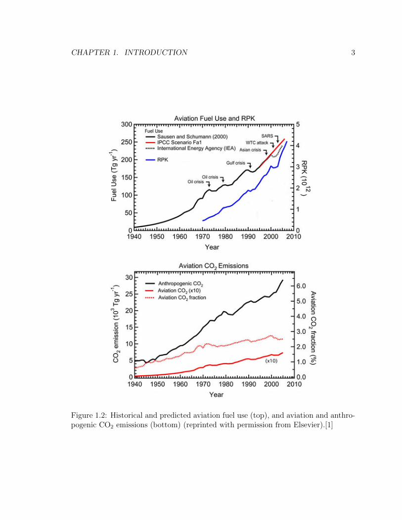
1.2 Historical and predicted aviation fuel use (top), and aviation and an-
thropogenic CO2 emissions (bottom) (reprinted with permission from
Elsevier).[1] . . . . . . . . . . . . . . . . . . . . . . . . . . . . . . . . 3
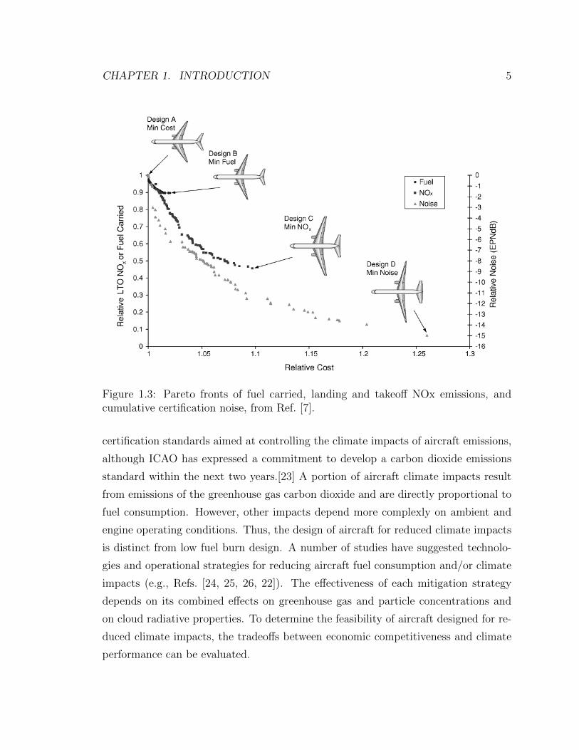
1.3 Pareto fronts of fuel carried, landing and takeoff NOx emissions, and
cumulative certification noise, from Ref. [7]. . . . . . . . . . . . . . . 5
2.1 Products of aircraft fuel combustion, adapted from Ref. [8]. . . . . . . 8
2.2 Schematic diagram of relationship between aircraft emissions and cli-
mate impacts (reprinted with permission from Elsevier).[1] . . . . . . 10
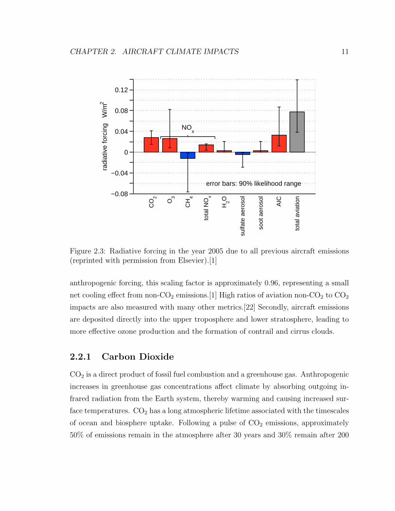
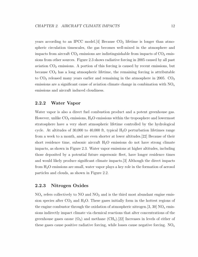
2.3 Radiative forcing in the year 2005 due to all previous aircraft emissions
(reprinted with permission from Elsevier).[1] . . . . . . . . . . . . . . 11
3.1 Cause and effect chain for aircraft climate change.[9] . . . . . . . . . 22
3.2 Graphical representation of the steps for calculating ATR. In this ex-
ample, H = 30 years, r = 3%, and tmax = 500 years. . . . . . . . . . . 33
4.1 Structure of PASS, adapted from Ref. [7]. . . . . . . . . . . . . . . . 36
4.2 Relationship between fan diameter, fan pressure ratio, and bypass ratio
for a turbofan engine.[10] . . . . . . . . . . . . . . . . . . . . . . . . . 38
4.3 Ideal propulsive efficiency versus fan pressure ratio.[11] . . . . . . . . 39
xiv

4.4 Effect of changing fan diameter on drag, weight, and propulsive effi-
ciency, adapted from Ref. [10]. . . . . . . . . . . . . . . . . . . . . . . 39
4.5 Comparison of fan sizes for turboprop, propfan, and turbofan engines
(reproduced with permission of the American Institute of Aeronautics
and Astronautics).[12] . . . . . . . . . . . . . . . . . . . . . . . . . . 40
4.6 Maximum available thrust versus Mach number at varying altitude for
turbofans and dual and single rotor propfans of varying bypass ratio. 43
4.7 Installed specific fuel consumption and overall efficiency versus throttle
setting for turbofans and propfans of varying bypass ratio. . . . . . . 44
4.8 Comparison of available thrust and specific fuel consumption for high
bypass ratio engines, from model predictions and a NASA study.[13] . 45
4.9 Engine length as a function of sea level static thrust. . . . . . . . . . 47
4.10 Nacelle form factor versus fineness ratio. . . . . . . . . . . . . . . . . 48
4.11 Variation in turbofan weight with sea level static thrust and fan diameter. 50
4.12 Turbofan and single and dual rotor propfan dry weight versus fan di-
ameter for 25,000 sea level static thrust engines. . . . . . . . . . . . . 52
5.1 Cruise and sea level static NOx emissions index for a sea level static
overall pressure ratio 41 turbofan engine predicted by equation (5.4). 60
5.2 Radiative forcing factor data for NOx impacts and aviation induced
cloudiness, based on results from Refs. [14] and [15]. . . . . . . . . . . 63
5.3 Scaled temperature impulse response functions from Hasselmann et al.,
Joos et al., Shine et al., and Boucher and Reddy.[16, 17, 18, 19] . . . 69
5.4 Forcing factors (lines) with 66% likelihood ranges (shaded areas). Al-
titudes with forcing factors based on raditiave forcing data with inde-
pendent probability distributions are marked with black points. . . . 75
6.1 Baseline designs optimized for minimum total operating costs and ATR
with two devaluation rates, r = 0 and r = 3%. Black points indicate
designs with listed cruise altitudes and Mach numbers. . . . . . . . . 85
6.2 Designs optimized for minimum total operating costs and ATRr=0,
applying propfan engines with varying assumptions. . . . . . . . . . . 88
xv

6.3 A natural laminar flow narrowbody aircraft design from Ref. [20]. . . 90
6.4 Designs optimized for minimum total operating costs and ATRr=0,
applying natural laminar flow with varying assumptions. . . . . . . . 91
6.5 Designs optimized for minimum total operating costs and ATRr=0,
applying biojet fuels with varying assumptions. . . . . . . . . . . . . 94
6.6 Designs optimized for minimum total operating costs and ATRr=0,
applying low NOx combustor technology with varying assumptions. . 96
6.7 Designs optimized for minimum total operating costs and ATRr=0,
applying a contrail avoidance strategy with varying assumptions. . . . 99
6.8 Pareto front of normalized total operating cost and ATR with separate
low contrails, NOx, and fuel burn technologies (each applied individually).100
6.9 Pareto front of normalized total operating cost and ATR with combi-
nations of low contrails, NOx, and fuel burn technologies. . . . . . . . 103
6.10 Pareto front of normalized total operating cost and ATR, showing 66%
confidence intervals for reduction in ATR relative to the reference design.106
6.11 Pareto front of normalized total operating cost and CO2 emissions
with climate impact reduction technologies. Evaluations of ATRr=0
and ATRr=3 are also shown. . . . . . . . . . . . . . . . . . . . . . . . 111
6.12 Pareto front of normalized total operating cost and ATR with mitiga-
tion technologies and lower (left) and higher (right) fuel prices. . . . . 113
6.13 Pareto front of normalized total operating cost and ATR with designs
optimized over a long range mission. . . . . . . . . . . . . . . . . . . 114
6.14 Pareto front of normalized total operating cost and ATR for designs
with fixed configuration parameters representing conventional aircraft
in the current fleet. . . . . . . . . . . . . . . . . . . . . . . . . . . . . 115
A.1 Diagram of engine station numbering, adapted from Ref. [21]. . . . . 124
A.2 Flow velocities through single and dual rotation propellers. . . . . . . 133
A.3 Fan polytropic and propulsive efficiencies as functions of fan pressure
ratio for dual rotor and rotor-stator fan configurations. . . . . . . . . 138
xvi

Chapter 1
Introduction
1.1 Global Climate Change
A 2007 assessment of global climate change estimates that surface temperatures in-
creased by 0.76C between the years of approximately 1875 and 2003, with simulta-
neous increases in ocean temperature, global sea levels, and melting snow and ice.[4]
The Intergovernmental Panel on Climate Change (IPCC) concluded that it is very
likely (more than 90% probability) that most of the observed temperature rise is due
to anthropogenic increases in greenhouse gas concentrations such as carbon dioxide.[4]
Depending on future emissions, temperatures are expected to rise an additional 1.5-
3.4C by the end of the century, as shown in Figure 1.1. The IPCC describes the
increasing likelihood of significant impacts on water availability, food production,
coastal flooding, and ecosystems as higher temperatures are reached.[6] Examples of
predicted consequences from temperature increases of more than 2C include the ex-
posure of millions of people to annual coastal flooding and increased risk of extinction
of up to 30% of species.
A small but growing portion of global climate change is attributed to the avi-
ation industry. In 2005, aircraft operations produced about 5% of the worldwide
anthropogenic forcing that causes climate change.[1] Many predict that commercial
aviation growth will continue to outpace improvements in efficiency, causing greater
forcings over the next several decades.[1, 3, 22] Figure 1.2 depicts historical aviation
1

CHAPTER 1. INTRODUCTION 2
Figure 1.1: Observed global average surface temperature rise during the 20th century(black) and global climate model projections of future temperature rise for varyingemissions scenarios (other colors), from Ref. [6].
fuel use and airline traffic and indicates strong growth since the beginning of the
jet age despite numerous disruptive events, including the September 11, 2001 ter-
rorist attacks.[1] Aviation fuel use growth has exceeded that of other industries, as
illustrated by the increasing aviation carbon dioxide emissions fraction in Figure 1.2.
Aviation induced climate change results not only from the release of carbon diox-
ide, but also from emissions of nitrogen oxides, water vapor, and particles and from
the effects of altered cloudiness. Of the climate forcing caused by aviation in 2005, car-
bon dioxide emissions produced forcing of 0.028 W/m2 (with a 90% likelihood range
of 0.015-0.041), while other emissions caused forcing of 0.049 W/m2 (0.013-0.110).[1]
Non-carbon dioxide forcing is caused almost entirely by nitrogen oxide emissions and
cloud effects; crucially, these impacts vary significantly depending on an aircraft’s
cruise altitude. These sensitivities must be considered when assessing aircraft cli-
mate impacts.
CHAPTER 1. INTRODUCTION 3
Figure 1.2: Historical and predicted aviation fuel use (top), and aviation and anthro-pogenic CO2 emissions (bottom) (reprinted with permission from Elsevier).[1]

CHAPTER 1. INTRODUCTION 4
1.2 Aviation and the Environment
As the aviation industry continues to grow, so too have concerns over the environmen-
tal impacts of aircraft. Among these impacts are community noise exposure, degraded
air quality in the vicinity of airports, and climate change from aviation greenhouse gas
emissions and the alteration of cloud properties. The public has expressed objections
to noise exposure since the industry’s beginnings, but recent attention has shifted
toward limiting aviation’s effects on the global climate. The combination of greater
public awareness, a rising number of individual airport regulations, and increasingly
stringent international standards has created important environmental constraints in
the design and operation of aircraft.
All aircraft certified since the 1980s have been required to meet environmental
standards set by the International Civil Aviation Organization (ICAO) for commu-
nity noise and emissions near airports.[23] The design relationships between aircraft
operating costs, fuel consumption, community noise, and local airport emissions were
investigated by Antoine.[7] Figure 1.3 compares the relative performance of aircraft
designed to minimize a combination of operating costs and environmental objectives.
Each point on the figure represents a unique aircraft design. Wing, engine, and
mission design parameters were varied in these studies to achieve improved environ-
mental performance relative to a minimum operating cost aircraft configuration. This
research quantified both the potential improvements in environmental performance
and associated penalties in terms of increased operating costs. In the figure, noise
margin and landing and takeoff nitrogen oxide emissions (LTO NOx) metrics quan-
tify environmental impacts in terms of ICAO regulatory measurements. Certification
noise and emissions reductions of up to 15 decibels and 50%, respectively, were pre-
dicted alongside 10-25% increases in operating costs. These results also demonstrate
the tradeoff between competing environmental constraints: for instance, designing
exclusively for minimal LTO NOx emissions leads to aircraft configurations with in-
creased fuel consumption and noise levels.
Antoine’s research explored opportunities for improved environmental performance,
focusing on regulated impacts from noise and local emissions. At present, there are no
CHAPTER 1. INTRODUCTION 5
Figure 1.3: Pareto fronts of fuel carried, landing and takeoff NOx emissions, andcumulative certification noise, from Ref. [7].
certification standards aimed at controlling the climate impacts of aircraft emissions,
although ICAO has expressed a commitment to develop a carbon dioxide emissions
standard within the next two years.[23] A portion of aircraft climate impacts result
from emissions of the greenhouse gas carbon dioxide and are directly proportional to
fuel consumption. However, other impacts depend more complexly on ambient and
engine operating conditions. Thus, the design of aircraft for reduced climate impacts
is distinct from low fuel burn design. A number of studies have suggested technolo-
gies and operational strategies for reducing aircraft fuel consumption and/or climate
impacts (e.g., Refs. [24, 25, 26, 22]). The effectiveness of each mitigation strategy
depends on its combined effects on greenhouse gas and particle concentrations and
on cloud radiative properties. To determine the feasibility of aircraft designed for re-
duced climate impacts, the tradeoffs between economic competitiveness and climate
performance can be evaluated.
CHAPTER 1. INTRODUCTION 6
1.3 Contributions and Outline
In order to limit damages from climate change, improvements may be necessary in
aircraft environmental performance. Extending the work of Antoine, this research
develops a framework for quantifying and comparing the climate performance of fu-
ture aircraft configurations using a conceptual design tool. Methods are presented for
aggregating the time-varying climate effects of aircraft fleets into a single, meaning-
ful metric. An integrated approach is taken, assessing how design changes influence
operating costs, fuel consumption, emissions rates, induced climate change, and basic
aircraft performance. The effects of climate impact reduction technologies are inves-
tigated, revealing several design and operation strategies for drastically reducing the
climate impacts of future aircraft.
A brief thesis outline is as follows. Chapter 2 describes the effects of aircraft emis-
sions on global climate and approaches to modeling emissions and climate impacts.
Chapter 3 discusses climate metrics and proposes the average temperature response
metric for aircraft design studies. Chapter 4 considers aircraft performance analysis
methods, including a new variable bypass ratio turbofan and propfan engine model.
Chapter 5 presents a linear, altitude-varying climate model that can be integrated
with an aircraft conceptual design tool. Chapter 6 discusses aircraft design studies
and explores the benefits of aircraft climate mitigation strategies. Finally, Chap-
ter 7 summarizes key conclusions and contributions of this research. A number of
opportunities for future research are also mentioned.

Chapter 2
Aircraft Climate Impacts
2.1 Introduction
Concern regarding aviation’s environmental impacts has grown during the last several
decades, leading to the development of international regulations on noise and emis-
sions in the vicinity of airports. More recently, the impacts of aircraft emissions on
global climate have attracted attention. Commercial aircraft operations affect the at-
mosphere and climate through emissions of greenhouse gases and their precursors and
through the formation of contrails and cirrus clouds. Since the majority of emissions
are released at high altitudes, these effects are not currently regulated. Assessments
of aviation’s climate impacts began in the late 1990s, culminating with the IPCC Spe-
cial Report, Aviation and the Global Atmosphere.[27, 3] Knowledge of aircraft climate
impacts improved following numerous research programs, and in 2009, the qualitative
and quantitative conclusions of the IPCC report were comprehensively updated.[1, 22]
Aviation emissions in 2005, including the highly uncertain effects of induced cirrus
cloudiness, were responsible for about 5% of all anthropogenic radiative forcing,[1]
which measures the net radiation imbalance at the top of the atmosphere due to a
perturbation. Based on the industry’s current trajectory, aviation radiative forcing is
predicted to grow by a factor of 3.0-4.0 between 2000 and 2050.[1] To determine the
effects of future aircraft operations on climate, methods are needed to estimate total
aircraft emissions and to model resulting climate impacts. This chapter first discusses
7

CHAPTER 2. AIRCRAFT CLIMATE IMPACTS 8
Air:
N2 + O2
Fuel:
CnHm + S
Ideal Combustion:
CO2 + H2O + N2 + O2 + SOX
Real Combustion:
CO2 + H2O + N2 + O2 + SOX +
UHC + CO + soot + NOX
Figure 2.1: Products of aircraft fuel combustion, adapted from Ref. [8].
the effects of aircraft operations on climate and next describes emissions and climate
models of varying complexity and accuracy.
2.2 Aircraft Emissions and Climate
Commercial aircraft engines are powered by the combustion of a hydrocarbon fuel,
the byproducts of which affect global climate. Jet A-1 fuel has an average carbon-
hydrogen ratio of C12H23 and contains approximately 400 parts per million by mass of
sulfur.[22, 28] The fuel is combusted to ideally produce carbon dioxide (CO2), water
vapor (H2O), and sulfur oxides (SOx). The mass of CO2, H2O, and SOx emitted per
kilogram of burned fuel depends on the exact fuel composition. Total annual emissions
from the global commercial fleet in 2006 are listed in Table 2.1.[2] In real combustion,
trace amounts of unburned hydrocarbons (UHC), carbon monoxide (CO), soot, and
nitrogen oxides (NOx) are also released, as given in Figure 2.1.[3] Emission rates for
these species are small compared with CO2 and H2O rates, as indicated in Table
2.1 Of these combustion products, CO2, H2O, NOx, SOx, and soot each directly or
indirectly alter the radiative balance of the Earth system over different timescales.
The IPCC and other groups have published extensive reviews of aviation’s climate
impacts.[27, 3, 29, 1, 22] Figures 2.2 and 2.3 provide overviews of aviation induced

CHAPTER 2. AIRCRAFT CLIMATE IMPACTS 9
Species Emission Quantity
CO2 emissions (Tg C) 162.25
H2O emissions (Tg H2O) 232.80
NOx emissions (Tg NO2) 2.656
CO emissions (Tg CO) 0.679
SOx emissions (Tg S) 0.111
HC emissions (Tg CH4) 0.098
Organic particulate matter emissions (Tg) 0.0030
Sulfur particulate matter emissions (Tg) 0.0023
Black carbon particulate matter emissions (Tg) 0.0068
Table 2.1: Annual emissions from global commercial aviation in 2006.[2]
climate change. Figure 2.2 shows the relationship between aircraft emissions, atmo-
spheric composition, radiative forcing, climate change, and impacts.[1] When con-
centrations of greenhouse gases and particles are perturbed, the balance of incoming
solar and outgoing infrared radiation is altered, causing radiative forcing. Forcing in-
fluences climate properties, such as temperature, precipitation, and extreme weather
events. These changes in climate affect many systems, including availability of food,
water, and energy. Finally, impacts can be translated into damages to social welfare.
The relative importance of each aircraft emission species depends on the chosen cli-
mate metric, but radiative forcing is often used by the IPCC. Figure 2.3 shows the
instantaneous radiative forcing experienced in 2005 due to aircraft emissions since
the beginning of the jet age in the 1940s.[1] The current, consensus scientific under-
standing of radiative forcing sources listed in Figure 2.3 are described in the following
sections. It should be noted that in the future, as knowledge is gained, conclusions
about the magnitudes and types of radiative forcing caused by aircraft emissions are
likely to change.
Climate impacts from aviation emissions differ from those of ground source emis-
sions in two key ways. First, the ratio of non-CO2 to CO2 impacts for aviation
emissions is significantly greater than the same ratio for ground source emissions.
For instance, using instantaneous forcing in 2005 shown in Figure 2.3, non-CO2 emis-
sions extend CO2 radiative forcing by a factor of 2.8; by comparison, for all global

CHAPTER 2. AIRCRAFT CLIMATE IMPACTS 10
chemical reactions
changes in temperatures, sea level, ice/snow cover, precipitation, etc.
ocean uptake
CO2 NOX H2O SOX HC soot
microphysical processes
ΔCO2 ΔCH4 ΔO3 ΔH2O Δaerosol contrails
agriculture and forestry, ecosystems, energy production and consumption, human health, social effects, etc.
social welfare and costs
Δclouds
Direct emissions
Atmospheric processes
Changes in radiative forcing
components
Climate change
Impacts
Damages
Figure 2.2: Schematic diagram of relationship between aircraft emissions and climateimpacts (reprinted with permission from Elsevier).[1]
CHAPTER 2. AIRCRAFT CLIMATE IMPACTS 11
−0.08
−0.04
0
0.04
0.08
0.12
CO
2
O3
CH
4
tota
l NO
x
H2O
sulfa
te a
eros
ol
soot
aer
osol
AIC
tota
l avi
atio
n
radi
ativ
e fo
rcin
g W
/m2
NOx
error bars: 90% likelihood range
Figure 2.3: Radiative forcing in the year 2005 due to all previous aircraft emissions(reprinted with permission from Elsevier).[1]
anthropogenic forcing, this scaling factor is approximately 0.96, representing a small
net cooling effect from non-CO2 emissions.[1] High ratios of aviation non-CO2 to CO2
impacts are also measured with many other metrics.[22] Secondly, aircraft emissions
are deposited directly into the upper troposphere and lower stratosphere, leading to
more effective ozone production and the formation of contrail and cirrus clouds.
2.2.1 Carbon Dioxide
CO2 is a direct product of fossil fuel combustion and a greenhouse gas. Anthropogenic
increases in greenhouse gas concentrations affect climate by absorbing outgoing in-
frared radiation from the Earth system, thereby warming and causing increased sur-
face temperatures. CO2 has a long atmospheric lifetime associated with the timescales
of ocean and biosphere uptake. Following a pulse of CO2 emissions, approximately
50% of emissions remain in the atmosphere after 30 years and 30% remain after 200
CHAPTER 2. AIRCRAFT CLIMATE IMPACTS 12
years according to an IPCC model.[4] Because CO2 lifetime is longer than atmo-
spheric circulation timescales, the gas becomes well-mixed in the atmosphere and
impacts from aircraft CO2 emissions are indistinguishable from impacts of CO2 emis-
sions from other sources. Figure 2.3 shows radiative forcing in 2005 caused by all past
aviation CO2 emissions. A portion of this forcing is caused by recent emissions, but
because CO2 has a long atmospheric lifetime, the remaining forcing is attributable
to CO2 released many years earlier and remaining in the atmosphere in 2005. CO2
emissions are a significant cause of aviation climate change in combination with NOx
emissions and aircraft induced cloudiness.
2.2.2 Water Vapor
Water vapor is also a direct fuel combustion product and a potent greenhouse gas.
However, unlike CO2 emissions, H2O emissions within the troposphere and lowermost
stratosphere have a very short atmospheric lifetime controlled by the hydrological
cycle. At altitudes of 30,000 to 40,000 ft, typical H2O perturbation lifetimes range
from a week to a month, and are even shorter at lower altitudes.[22] Because of their
short residence time, subsonic aircraft H2O emissions do not have strong climate
impacts, as shown in Figure 2.3. Water vapor emissions at higher altitudes, including
those deposited by a potential future supersonic fleet, have longer residence times
and would likely produce significant climate impacts.[3] Although the direct impacts
from H2O emissions are small, water vapor plays a key role in the formation of aerosol
particles and clouds, as shown in Figure 2.2.
2.2.3 Nitrogen Oxides
NOx refers collectively to NO and NO2 and is the third most abundant engine emis-
sion species after CO2 and H2O. These gases initially form in the hottest regions of
the engine combustor through the oxidation of atmospheric nitrogen.[3, 30] NOx emis-
sions indirectly impact climate via chemical reactions that alter concentrations of the
greenhouse gases ozone (O3) and methane (CH4).[22] Increases in levels of either of
these gases cause positive radiative forcing, while losses cause negative forcing. NOx

CHAPTER 2. AIRCRAFT CLIMATE IMPACTS 13
emissions also affect climate through the formation of particulate nitrate;[31, 4] how-
ever, the associated negative radiative forcing is very uncertain and is not modeled
in this research.
First, NOx emissions produce positive forcing by increasing concentrations of O3,
which has a chemical lifetime on the order of several weeks.[22] The cause of this O3
perturbation is twofold. Ozone production rate is enhanced as NO emissions convert
to NO2, which photolyzes to produce atomic oxygen, then reacts with molecular
oxygen to produce O3. Additionally, the O3 loss rate decreases due to lower abundance
of the peroxy radical, which is consumed in the conversion of NO to NO2.[22] NOx
emissions in the mid-latitude upper troposphere and lower stratosphere produce O3
more efficiently in terms of molecules of O3 per molecule of NO than anywhere in the
atmosphere.[3] Assessments of these short-lived effects indicate increased NOx and O3
concentrations of 30-40% and 3%, respectively, near flight corridors.[22] It should be
noted that NOx emissions in the stratosphere, for instance from supersonic aircraft,
cause net O3 destruction. The crossover altitude where NOx emissions convert from
net O3 production to destruction is estimated to be near 16 km, or 52,000 ft.[22]
Secondly, NOx emissions accelerate the rate of destruction of ambient CH4 over
longer timescales on the order of 12 years. Associated with this process is low magni-
tude, long-term ozone destruction. Because these cooling impacts occur over decades,
their forcings become mixed on a hemispheric scale, in contrast with short-term ozone
production forcing that remains concentrated near flight routes. The warming, cool-
ing, and net impacts of NOx emissions in the year 2005 from all past aviation emissions
are illustrated in Figure 2.3.[1] As noted previously, short-term impacts shown in this
chart result only from recent emissions, while long-term forcing includes forcing from
all remaining past perturbations.
2.2.4 Sulfur Oxides
Aviation fuel contains a small percentage of sulfur, most of which is oxidized to sulfur
dioxide (SO2) in the combustor. A fraction of this SO2 is further oxidized via gas phase
chemical reactions inside the engine and plume to sulfur trioxide (SO3) and sulfuric

CHAPTER 2. AIRCRAFT CLIMATE IMPACTS 14
acid (H2SO4). Liquid particles of H2O and H2SO4 form via homogeneous nucleation,
and they grow in size by coagulation and condensation processes. The result is an
increase in sulfate aerosol number and area density near flight routes. Sulfate particles
scatter incoming solar radiation and absorb very little outgoing infrared radiation,
leading to a net cooling impact. Sulfate aerosol production from aircraft is small
relative to surface and volcanic sources, and these particles have very short lifetimes
of approximately four days.[3, 32] Figure 2.3 illustrates the small direct impact from
sulfate aerosol emissions, but sulfate particles also play a role in the formation of
contrail and cirrus clouds.[1]
2.2.5 Soot Particles
Carbon soot particles containing graphite carbon and organic compounds form in
aircraft engine combustors. Emission rates vary in a complex manner with combustor
operating conditions and design but generally increase with engine throttle setting.[33]
The development of engine emissions regulations has lowered soot emission rates,
demonstrated by modern engine emission rates that are 40 times lower than those
of 1960s engines.[1] Total annual commercial aviation emission rates for organic and
black soot particulate matter in the year 2006 are listed in Table 2.1. Soot absorbs
solar radiation very effectively, producing the small warming effect shown in Figure
2.3. Like sulfate particles, the atmospheric lifetimes of soot particles are very short,
on the order of approximately one week.[32] On average, the direct impacts of soot
particles are small, but these particles can also serve as nucleation sites for contrail
particles. A recent global climate model assessment concluded that direct impacts
from aviation soot emissions could be greater than previously expected, particularly
in the Arctic circle.[34]
2.2.6 Aviation Induced Cloudiness
Aviation induced cloudiness (AIC) includes the formation of linear contrails, aged
contrail-cirrus, and soot cirrus clouds. These clouds reflect incoming solar radia-
tion and trap outgoing infrared radiation, producing a net positive radiative forcing
CHAPTER 2. AIRCRAFT CLIMATE IMPACTS 15
on average. The magnitude of forcing caused by individual clouds varies diurnally,
with nighttime contrails causing considerably greater warming effects than daytime
contrails.[35] The impacts of these phenomena are very uncertain, particularly for
contrail-cirrus and soot cirrus.
Linear condensation trails, or contrails, form when hot, moist air in the engine
exhaust mixes with sufficiently cool ambient air. The threshold temperature for con-
trail formation is determined by the Schmidt-Appleman criterion, which describes
whether liquid saturation is reached within the young aircraft plume in terms of am-
bient and exhaust temperatures and water content. If temperature conditions are
met, water vapor condenses onto exhaust particles, and these liquid droplets freeze.
The radiative impacts of contrails are negligible unless the ambient air is supersatu-
rated with respect to ice, causing the contrail to persist for as long as the air remains
ice-supersaturated, often several hours.[36] Conditions for persistent contrail forma-
tion can exist between the altitudes of 20,000 and 45,000 ft, with a peak frequency
of about 15% at 30,000 ft altitude.[15] Approximately one-third of the AIC forcing
shown in Figure 2.3 is attributed to linear contrails. However, there is significant
uncertainty in quantifying net contrail impacts, which depend on accurate models of
contrail coverage and optical depth.[1]
Aviation cirrus can be formed either from the spreading of linear contrails, known
as contrail-cirrus, or from the increase in the number of particles near cruise altitudes
that can act as cloud condensation nuclei, known as soot cirrus. Contrail-cirrus are
estimated to increase contrail coverage by a factor of 1.8, although estimates of its
addition to forcing are highly uncertain. Uncertainties in quantifying forcing due to
soot cirrus are even greater. Soot cirrus includes the alteration of ambient cloud
properties and the formation of new cirrus clouds. It is currently not known whether
net soot cirrus forcing is positive or negative. Aviation cirrus impacts are sometimes
excluded from overall aviation forcing estimates due to their high uncertainty; how-
ever, these impacts and their uncertainties are included in this research. Figure 2.3
estimates the net total forcing due to all three components of aviation cloudiness,
and this value is derived from correlation analyses of cloud coverage and air traffic by
assuming cloud properties similar to thin cirrus.[1]

CHAPTER 2. AIRCRAFT CLIMATE IMPACTS 16
2.3 Aircraft Emissions Regulations
Industry-wide environmental standards are developed for commercial aviation by the
International Civil Aviation Organization (ICAO) through its Committee on Aviation
Environmental Protection (CAEP). For an aircraft engine to be certified, it must meet
landing and takeoff emissions standards designed to protect air quality near airports.
These regulations apply to engine certification and do not account for total aircraft
emissions; thus, within this regulatory framework, aircraft with greater sea level static
thrust can have higher overall emissions rates, irrespective of differences in payload
or range. At present, there are no ICAO regulations limiting cruise emissions, but
future policies to limit climate impacts are under consideration.[23]
Landing and takeoff (LTO) emissions standards exist for NOx, CO, UHC, and
soot (as measured by smoke number). Of these pollutants, only NOx emissions pro-
duce significant climate impacts. Regulations for NOx emissions have been made
increasingly stringent over the past three decades and CAEP6 limits are currently in
effect.[23] These regulations limit the total mass of emissions released per unit thrust
during a landing-takeoff cycle, representing emissions below 3,000 ft. Emissions are
measured for simulated taxi, takeoff, climb out, and approach conditions. Standards
vary with engine pressure ratio, allowing engines with higher combustor pressures
and temperatures to emit more NOx. Emissions and fuel burn measurements for all
certified engines are published in the ICAO Emissions Databank.[37] Although only
landing and takeoff emissions are regulated, it is generally assumed that reductions
in LTO emissions are accompanied by reductions in cruise NOx.[22]
2.4 Emissions Modeling
Current emissions regulations target pollution during landing and takeoff only, but,
the majority of emissions are released above 3,000 ft altitude and these emission rates
are not included in ICAO Databank measurements. To determine the climate impacts
of a future aircraft fleet, emissions must be modeled over the entire mission. Different
methods of varying complexity exist for estimating emissions, but for conceptual

CHAPTER 2. AIRCRAFT CLIMATE IMPACTS 17
design, computationally efficient methods are needed. Following ICAO measurement
procedures, emission rates are described by the emissions index or the mass ratio of
emitted species to consumed fuel.
2.4.1 Fuel-Proportional Emissions
For many radiatively important species, total emissions are simply proportional to
fuel consumption. The mass of CO2, H2O, and SOx released per fuel burned is
determined from the composition of the fuel. These species have emissions indices
that are constant between different designs and over all operating conditions.
2.4.2 NOx P3-T3 Method
NOx emissions index, on the other hand, varies significantly with both engine design
characteristics and operating conditions. The formation of NOx in an aircraft engine
combustor involves unsteady physical processes and non-equilibrium chemical reac-
tions and is complex to model analytically.[38, 30, 3, 39] Empirical methods have been
developed based on experimental data to more simply relate emission rate to relevant
combustor parameters. These correlations estimate NOx emissions index based on
models of combustor residence time, chemical reaction rates, and mixing rates.[40]
For a fixed combustor design, emissions index can be estimated to a high degree of
accuracy (better than 5%) from combustor inlet temperature and pressure based on
experimental data.[3] Such models, referred to as P3-T3 methods, exist for numerous
conventional and advanced combustor configurations. An example of a P3-T3 model
is described in more detail in Chapter 5. These approximate methods greatly simplify
the estimation of NOx emission rate and do not capture all variations in emission rates
with changing conditions. Moreover, P3-T3 models are only accurate for the specific
combustor configuration for which the correlation is derived.
CHAPTER 2. AIRCRAFT CLIMATE IMPACTS 18
2.4.3 Fuel Flow Correlation Methods
NOx P3-T3 correlation methods rely on knowledge of combustor inlet temperature
and pressure for emissions index estimation. Information about the variation of these
parameters with operating condition requires proprietary information or detailed en-
gine models that may not be available for conceptual design studies or development
of emissions inventories. For this reason, more simple fuel flow correlation methods
have been developed. These methods compute NOx emissions index at any operating
condition based on ambient conditions, fuel flow rate, and publicly available ICAO
landing and takeoff certification data. Fuel flow correlations are less accurate than
P3-T3 methods but require less knowledge of detailed combustion parameters. Two
common methods, the Boeing Method 2 and DLR fuel flow correlations,[41, 42] have
been applied in numerous studies of aviation emissions.[43, 44, 8, 45, 46] These mod-
els replicate cruise emissions index measurements and P3-T3 predictions to within
approximately ±10%.[8]
Fuel flow correlation methods also exist for estimating cruise soot emissions index;[42]
however, direct soot climate impacts are small compared with aircraft CO2, NOx, and
aviation induced cloudiness. Therefore, soot emissions index is assumed to be con-
stant over all operating conditions without significant loss in accuracy for total climate
impact estimation. For detailed combustor technology studies, a more accurate model
for soot emissions would be necessary.
2.5 Climate Impact Modeling
A variety of model types are used to predict the impacts of past and future anthro-
pogenic activities on global climate. The IPCC recognizes the need for a spectrum of
models, each with a level of complexity and simulation quality appropriate for differ-
ent study applications.[4] This section describes three categories of climate models.
CHAPTER 2. AIRCRAFT CLIMATE IMPACTS 19
2.5.1 Global Climate Models
Global climate models (GCMs) are complicated mathematical representations of the
fluid dynamics and chemistry associated with the atmosphere, ocean, and land sur-
face. These programs vary in complexity and are used to predict the impacts of
anthropogenic emissions on climate. The most complex models are three-dimensional
coupled atmosphere-ocean general circulation models (AOGCMs), and 23 such mod-
els were applied in the recent IPCC Fourth Assessment Report.[4] Climate modeling
has advanced substantially over the last several decades: the IPCC stated that “there
is considerable confidence that climate models provide credible quantitative estimates
of future climate change, particularly at continental scales and above.”[4] This con-
fidence arises from the fundamental principles upon which models are based and
their ability to reproduce observations of past and present climate change.[4] How-
ever, global climate models are computationally expensive, taking weeks or months
to evaluate.[47] As a result, global climate models are not well-suited for applications
requiring multiple calculations, such as uncertainty evaluations or conceptual design
studies.[48]
2.5.2 Integrated Assessment Models
Integrated assessment models (IAMs) are tools developed to assess the environmen-
tal and economic system responses of prescribed anthropogenic activity scenarios.
These methods do not model the physical and chemical processes of climate change
as accurately as global climate models, but instead quantify global and regional eco-
nomic impacts.[49] Three commonly applied IAMs include the FUND, DICE, and
PAGE models. Each model converts emissions into concentration change, temper-
ature change, and finally social costs. Damage functions translate warming into
economic costs and rely on the climate modeling community’s best judgments, but
these representations are incomplete and highly uncertain.[50] IAMs are useful tools,
designed to inform climate change policy decisions.

CHAPTER 2. AIRCRAFT CLIMATE IMPACTS 20
2.5.3 Linear Temperature Response Models
Linear temperature response (LTR) models are simplified representations of the cli-
mate system based on results from global climate models. Instead of computing
concentrations, radiative forcing, and temperature change on a time-varying, three-
dimensional global grid, most LTRs estimate globally- and annually-averaged con-
ditions. LTRs are less accurate than GCMs but are expected to capture first order
effects from emissions and have the useful properties of computational efficiency,
transparency, and flexibility to incorporate new knowledge.[51, 52] As a result, LTRs
are valuable for aviation studies, and especially conceptual design optimization stud-
ies where many emissions scenarios must be considered. Because of their low com-
putational costs, uncertainty analysis can be performed with LTRs to determine the
degree of confidence in result estimates.
LTRs have been developed for numerous past aviation studies.[51] Sausen and
Schumann applied a linear model based on the response functions of Hasselmann et
al. to compare the effects of CO2 and NOx emissions.[53, 54] More recently, Marais
et al. developed the Aviation Environmental Portfolio Management Tool, which es-
timates not only temperature change, but also damages based on linear response
functions.[55] Lim et al. apply the LinClim tool, which is similar to the model of
Sausen and Schumann, but includes the effects of more emissions species.[47] Finally,
the LTR AirClim, developed by Grewe and Stenke, computes impacts based on effects
over a coarse global grid with varying impact intensities.[56] A linear temperature re-
sponse model with similar elements to many of these methods and designed for use
in conceptual design studies is described in Chapter 5.
Chapter 3
Climate Change Metrics
3.1 Introduction
Given the significance of aviation climate change, it is important for the aircraft de-
sign community to have a meaningful method for measuring the climate impacts of
various aircraft configurations and technologies. This estimation must account for the
multiple radiatively active species that aircraft emit. Emissions of CO2, NOx, H2O,
SOx, and soot from fuel combustion alter both atmospheric composition and cloud
properties. The causal sequence of emissions to the impacts and damages caused by
climate change is shown in Figure 3.1. Atmospheric processes convert direct aircraft
emissions into chemicals and form clouds that change the balance of incoming and
outgoing energy in the Earth-atmosphere system, producing radiative forcing. Radia-
tive forcing components then cause climate change, manifested as changes to global
mean temperature, precipitation, sea level, etc. Next, climate change influences agri-
culture, coastal geography, and other systems. The likelihood of significant impacts
on these systems as a function of temperature rise is explored by the IPCC.[6] Finally,
climate change impacts can be quantified monetarily as damages or costs to society.
Along each step of the path shown in Figure 3.1, variables can be identified which
could serve as climate change metrics. Metrics based on lower steps in the figure are
increasingly relevant in quantifying the potential effects of climate change sought to
be avoided. However, these quantities are also increasingly uncertain and difficult to
21

CHAPTER 3. CLIMATE CHANGE METRICS 22
Direct Emissions:
CO2 , NOx , H2O, SO4 , soot
Changes in Radiative
Forcing Components:
∆CO2 , ∆CH4 , ∆O3 , ∆H2O,
∆aerosols, ∆clouds
Climate Change:
Changes in temperature,
sea level, precipitation, etc.
Impacts:
Agriculture and forestry,
ecosystems, human health, etc.
Damages:
Social welfare and costs
Incr
easi
ng
un
cert
ain
ty
Incr
easi
ng
rele
van
ce
Figure 3.1: Cause and effect chain for aircraft climate change.[9]
predict. When selecting a metric for measuring climate change, one must balance the
relevance of the metric against the uncertainty its use leads to in making decisions.
In this chapter, first, metrics generally applied for different climate applications are
described. Next, the suitability of metrics for aircraft conceptual design are consid-
ered, and a methodology for estimating aircraft climate performance with a single
candidate metric is presented. The candidate metric, average temperature response,
can be combined with a simple climate model to provide a framework for assessing
relative performance of competing aircraft designs.
CHAPTER 3. CLIMATE CHANGE METRICS 23
3.2 Commonly Used Climate Metrics
Several different metrics have been developed to quantify impacts from climate change.
Five of the most commonly used metrics are briefly described in this section: mass
of emissions, radiative forcing, global warming potential, global temperature poten-
tial, and damages. Applications for these metrics range from IPCC global scenario
assessments to individual sector studies to international policy analyses.
3.2.1 Mass of Emissions
One very simple metric quantifies climate effects in terms of the total mass of emis-
sions, usually CO2. Because CO2 has a long atmospheric lifetime and its impacts
are comparatively well understood, metrics based on mass of CO2 emissions can be
meaningful. However, for applications with numerous emission species of varying
atmospheric lifetimes, mass-based metrics are less useful.
3.2.2 Radiative Forcing
As previously noted, radiative forcing (RF) measures the net imbalance of incoming
and outgoing energy in the Earth-atmosphere system caused by a perturbation. RF
does not directly measure a change in climate behavior, but instead quantifies the
change in energy that produces changes in climate properties including temperature
and precipitation. However, under certain restrictive assumptions, RF is directly
related to changes in equilibrium surface temperature.[3] While RF is usually reported
as a snapshot at a single time, RF can also be used as a time-varying climate metric.
RF metrics have been applied extensively in climate change research, including studies
by the IPCC.[3]
3.2.3 Global Warming Potential
Global warming potential (GWP) is defined as the time-integrated RF caused by a
pulse emission of a particular forcing agent over a specified time period, normalized by
the time-integrated RF due to a pulse emission of CO2 over the same specified period.
CHAPTER 3. CLIMATE CHANGE METRICS 24
Alternatively, sustained GWPs may also be defined based on continuous emissions
over a specified time horizon. Different time periods may be considered, but 100 years
is commonly used and was adopted by the United Nations Framework Convention
on Climate Change for the Kyoto Protocol. GWPs have been widely reported for
long-lived gases including CO2. More recently, GWPs for short-term perturbations
from NOx emissions and AIC effects have been published, although these potentials
are more difficult to quantify.[32]
3.2.4 Global Temperature Potential
Global temperature potential (GTP) quantifies the ratio of global mean temperature
changes resulting from equal mass emissions of CO2 and another species.[18, 28, 57]
GTP is a snapshot metric that evaluates temperature change at a single point at
the end of a time horizon, rather than evaluating time-integrated impacts. Similar to
GWPs, GTP emissions scenarios may be based on either pulse or sustained emissions.
Lastly, GTPs can be calculated with any climate model, but simplified linear climate
models are often used.[28]
3.2.5 Damages and Other Economic Metrics
Economic metrics evaluate the damages and abatement costs of different emissions
scenarios. Integrated assessment model studies, described in Chapter 2, usually quan-
tify impacts in economic terms (e.g., Refs. [58, 59, 60, 55]). These metrics are par-
ticularly useful for aggregating impacts of varying type and location to inform policy
decisions. Still, there are no approaches to estimating climate change impacts in
economic terms that are widely accepted by the climate change community.[51]

CHAPTER 3. CLIMATE CHANGE METRICS 25
3.3 Climate Metric for Comparative Aircraft De-
sign
Researchers have adopted numerous climate metrics to quantify the impacts of avia-
tion emissions, including those discussed in the previous section. The strengths and
weaknesses of these metrics are reviewed in Refs. [61, 18, 62, 63, 51, 52, 32, 28].
Many of these metrics have been applied extensively to the comparison of impacts
from different sectors, the prediction of impacts based on future emission scenarios,
and the assessment of various technology and policy mitigation strategies. In or-
der to compare the climate impacts of different aircraft designs, a metric is needed
that appropriately characterizes the net global climate effect of operation of a fleet
of particular aircraft. To narrow the set of possible aircraft design climate metrics,
discussion will focus on the appropriate properties of a metric for this purpose. Then,
a candidate metric for comparative aircraft design is presented.
3.3.1 Desired Metric Properties
Measured Quantity A climate metric could measure many different physical or
economic values, ranging from mass of emissions to radiative forcing to temperature
change to impacts and damages, as shown in Figure 3.1. For estimating the impacts of
aircraft operations, the mass of radiatively active emissions is not a meaningful metric
because of the wide variety of aircraft emissions that affect climate. For example, the
timescales and intensity of climate impacts due to emissions of one kilogram of CO2
are very different from those of one kilogram of NOx; furthermore, AIC impacts are
not simply related to a single emissions quantity. Because of this, emissions quantity
metrics are less useful for aircraft design studies.
Economic metrics evaluate the damages and abatement costs of different emis-
sions scenarios. These economic metrics use damage functions that estimate the
effects of climate change in terms of the consumption-equivalent value of both market
and non-market goods.[50] Such models are highly uncertain: Nordhaus describes
the damage function in his model as “extremely conjectural given the thin base of
CHAPTER 3. CLIMATE CHANGE METRICS 26
empirical studies on which it rests.”[64] Uncertainty in estimating damages is more
challenging to quantify and greater in magnitude than that of physical metrics such
as radiative forcing and temperature change. Furthermore, temperature change is
a tangible measure of climate change that is more accessible than damage metrics,
and many policies focus on the objective of temperature rather than social damages.
For comparative studies, under certain restrictive assumptions described in Ref. [63],
conclusions drawn using global cost potential and global temperature potential met-
rics coincide. Additionally, because the purpose of this metric is for use in aircraft
design, and not policy decisions, economic metrics are not necessarily preferred. To
inform future policy decisions, it is important to measure each environmental impact
(noise, local emissions, and climate change) and understand how environmental and
economic performance can be changed in design. For these reasons, economic-based
metrics will not be used herein for comparative aircraft design study.
Other climate properties include radiative forcing and temperature change. Both
are physical quantities often noted in climate change studies. Unlike forcing, tem-
perature change is a direct measure of a change in global climate behavior. RF is
therefore a less direct measure of the level of impact of aircraft emissions. RF has the
advantage of lower scientific uncertainty compared with temperature change. The
primary limitation of RF is that it is an instantaneous metric which captures impacts
from emissions at a single point in time; however, time-integrated RF metrics can be
used to quantify lifetime impacts. Both radiative forcing and temperature change are
identified as potential candidates for the basis of an aircraft design climate metric.
Emissions Case Most climate metrics are computed based on a specified, general
emissions case. For instance, sustained 100 year GWPs are calculated assuming con-
stant emissions for 100 years while pulse 100 year GWPs are calculated assuming
emissions for only one year and zero emissions thereafter. GWPs are used broadly
for many applications and are also referenced for 20 year and 500 year horizons. For
the application of aircraft design, a more specific emissions case is appropriate. To
compare the impacts of different aircraft designs, climate impacts can be computed
with an emissions case representative of the likely operation of these designs. Based

CHAPTER 3. CLIMATE CHANGE METRICS 27
on typical commercial aircraft operation today, an appropriate emissions case might
be constant operation for 30 years followed by aircraft retirement and zero emissions
(other operating lifetimes could be considered for different aircraft design applica-
tions). The scenario of constant emissions during the operational lifetime and zero
emissions thereafter is a simplistic representation of the emissions from a new aircraft
design – in reality, new aircraft are adopted gradually and the net emissions rates
from the new design change annually. However, this simple emissions case is suffi-
cient to capture the differences in lifetime climate impacts in a comparative design
study.
Snapshot vs. Integrated Impact A climate metric can be based on the evalua-
tion of a property at a single point in time or the integration of that property over a
period of time. Common snapshot metrics include single year RF and GTP, and com-
mon integrated metrics include GWP and integrated temperature change.[55, 32, 28]
For aircraft design, a snapshot metric can be applied at the end of the operating
lifetime, quantifying the value of a climate property near its peak value. Snapshot
metrics could also be applied within or after the operating lifetime if considering a
climate goal, for instance a temperature change target in the year 2050. It should
be noted that even for a comparative study, snapshot metrics are very sensitive to
timing, and a study with a lifetime of 10 years could give a different result than
that with a lifetime of 50 years. Time-integrated climate metrics are less sensitive to
lifetime and quantify mean impacts over an integration period. Because components
of RF and temperature change are accumulative and vary annually, lifetime-averaged
metrics are preferred for aircraft design studies.
Temporal Weighting Given an integrated impact metric based on the emissions
case described above, the relative importance of short-lived and long-lived impacts
can be altered by applying temporal weighting. Common methods for weighting in-
clude discounting and windowing, but other weighting functions can also be used.
Discounting is frequently used in economic studies to express future value in present

CHAPTER 3. CLIMATE CHANGE METRICS 28
monetary terms and has been applied in climate change studies.[65, 66, 55] In a sim-
ilar manner as discounting, weighting factors can be applied to a physical impact
to specify the relative importance of immediate and far future impacts. Integration
window also affects this balance by setting the maximum time horizon for inclusion
of impacts. Short-lived impacts decay quickly (10-30 years) after aircraft operations
terminate but long-lived impacts decay slowly (hundreds of years for CO2). There-
fore, an integration window that is long compared with the aircraft operating lifetime
favors long-lived impacts, while a short window biases toward short-lived impacts. A
weighting function can combine weighting factors and an integration window. Be-
cause choices of weighting represent judgments on the value of immediate and far
future impacts, an aircraft design climate metric should be flexible and allow of user
specification of the associated function.
Treatment of Uncertainty Considerable uncertainty exists in the quantification
of climate impacts from aircraft emissions and other sources. The relevant uncertainty
may be categorized as described in Ref. [67]. Scientific uncertainty is associated with
limits in scientific knowledge and inexact modeling approaches for estimating impacts
from an emissions scenario. Valuation uncertainty exists because value judgments are
required to temporally weight impacts. Scenario uncertainty refers to unknowns sur-
rounding the projections of future anthropogenic activities and system responses that
are required to estimate aircraft climate impacts. For an aircraft design climate met-
ric to be practical, scientific uncertainty must be quantifiable. The effects of scientific
uncertainties on design results can be quantified using the approach described in
Chapter 5. Scenario and valuation uncertainty should also be addressed by allowing
user specification of trajectory and temporal weight assumptions.
3.3.2 Average Temperature Response
Based on the discussion of the desired properties of an aircraft design climate metric,
several metrics could be conceived. One such metric, average temperature response,
is presented here. This metric is based on temperature change for several reasons.
First, temperature change is commonly used within the climate modeling community

CHAPTER 3. CLIMATE CHANGE METRICS 29
but is also understood by non-experts. Secondly, it measures a physical change in
climate behavior that could be controlled in order to limit climate change damages.
The purpose of the candidate metric is to quantify for a particular aircraft the climate
impacts realized from emissions during operation and also climate impacts that result
from perturbations remaining in the Earth-atmosphere system after the aircraft’s
operating lifetime has ended.
The metric presented in this study is the average temperature response (ATR)
over an aircraft’s operating lifetime. ATR combines integrated temperature change
with the concept of temporal weighting and follows the general emissions metric
formulation given in Refs. [4, 60]. Average temperature response is defined in equation
(3.1).
ATRH =1
H
∫ ∞0
∆Tsust,H(t)wr(t) dt (3.1)
ATR is measured in units of temperature. The first step in computing ATR is
calculating the global mean temperature change. In the above equation, ∆Tsust,H
refers to the time-varying global mean temperature change caused by H years of
sustained operation of a particular aircraft configuration. The function ∆Tsust,H(t) is
determined based on constant annual emissions rates for the first H years of CO2,
NOx, H2O, soot, and sulfate, and constant stage length, and zero emissions thereafter.
Aircraft operating lifetimes typically range between 25 and 35 years [3]. All studies
herein assume an operating lifetime (H) of 30 years.
Temperature change can be quickly calculated using a linear temperature response
model for aircraft conceptual design studies, or more sophisticated climate models can
be used. Linear methods calculate the time-varying temperature change from a set
of emissions using simplified expressions derived from the results of complex global
climate models. Linear models of varying complexity for aviation studies are applied
in Refs. [53, 47, 68, 56, 55, 1, 32].
Weighted temperature change per year is integrated and divided by H to yield
an average temperature response. Any unitless weighting function may be used, and
multiple functions could be appropriate for this purpose, including simple windowing

CHAPTER 3. CLIMATE CHANGE METRICS 30
and discounting.[65, 61, 18, 62, 4, 63, 51, 52, 32, 28] Window weighting functions
include only impacts occurring within a specified timeframe, and an example of their
application is the integrated radiative forcing metric GWP. Discounted metrics weight
future impacts with an exponentially decaying function using either a constant or
time-varying discount rate. Discount weighting functions are often applied in net
present value economic metrics but can also be applied to physical metrics for many
studies.[69] Conventional temporal weighting methods of windowing and discounting
can be applied to an aircraft design climate metric, but other functions can also
be used. To demonstrate this, the weighting function defined in equation (3.2) is
presented.
wr(t) =
1 t ≤ H
1(1+r)t−H
H < t ≤ tmax
0 t > tmax
(3.2)
This function assigns unity weighting to temperature change during the operating
lifetime of the aircraft. An exponential devaluation rate is applied to temperature
change occurring after the aircraft has ceased operation (t ≥ H). A rate of zero
means that post-operation impacts are equally important compared with impacts
during operating years; a rate of infinity means that post-operation impacts have no
importance; a positive, finite rate means that temperature change each post-operation
year is less important than the temperature change experienced the previous year. A
maximum integration window defined by tmax is also applied.
The function wr(t) is designed so that long-term effects are included but do not
dominate ATR. As described by the IPCC, the design of a reduced climate impact
next generation commercial aircraft and other short-term climate abatement decisions
involve “balancing the economic risks of rapid abatement now and the reshaping of
the capital stock that could later be proven unnecessary, against the corresponding
risks of delay.”[70] Designing an aircraft based on its climate impacts in 100 years
is higher risk than designing an aircraft based on its impacts in the next 30 years
because there is greater confidence that avoided climate change in the near-term
will be highly valued. The relative importance of a unit of temperature change in
CHAPTER 3. CLIMATE CHANGE METRICS 31
the far future is uncertain and unpredictable, and depends on future trajectories of
technological growth, realized physical impacts, and mitigation and adaptation. In
contrast, the value of short-term impacts are more certain. Short-term impacts are
defined here by the window of approximately 30 years, which coincides with the op-
erating lifetime of typical commercial aircraft. In equation (3.2), short-term impacts
are weighted at unity, and long-term effects are weighted with importance that decays
exponentially. Decaying weighting factors are delayed 30 years for two reasons. First,
as previously mentioned, scenario uncertainty is more moderate during this period:
emissions, technological change, and policy scenarios are more certain for the next
generation. Secondly, scientific uncertainty is lower during this period: results in Ref.
[4] indicate that during a 30 year window, predictions of temperature change reason-
ably agree not only within and across models, but also between emissions scenarios.
This weighting function and other monotonically decreasing functions are con-
sistent with approaching climate change abatement as a task of sequential decision
making under uncertainty.[70] The task is to design the next generation of commer-
cial aircraft with cost effective climate impact reduction solutions so that in 30 years,
climate change has not reached such high levels as to limit future options.[71] In the
meantime, technology advancement and learning will continue. For the design of the
following generation of aircraft, decisions will be better informed and aircraft climate
mitigation will be reevaluated.
Selection of the weighting function involves a value judgment of the relative im-
portance of short-lived and long-lived impacts. For the presented weighting function,
wr(t), the devaluation rate is provided as a user-specified value judgment. Tempera-
ture change caused by short-lived impacts decays quickly after operation stops while
long-lived species such as CO2 cause a residual temperature change for many years
post-operation. In aircraft design studies presented in Chapter 6, devaluation rates
of 0% and 3% are considered. The integration window is taken to be very large
compared with operating lifetime (if desired, shorter windows could also be used).
A finite window is required for very low rates because a fraction of CO2 emissions
remain in the atmosphere for many thousands of years and therefore most models
for CO2-induced temperature change do not decay to zero;[72] thus, for the case of
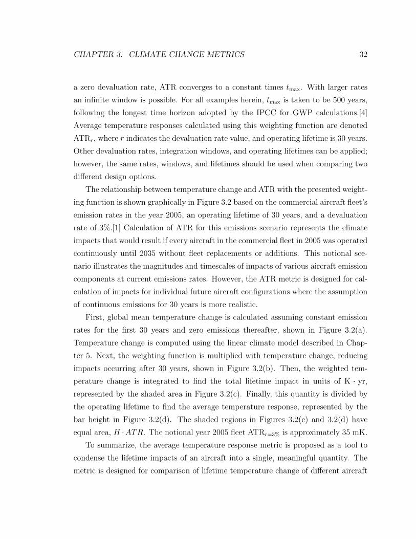
CHAPTER 3. CLIMATE CHANGE METRICS 32
a zero devaluation rate, ATR converges to a constant times tmax. With larger rates
an infinite window is possible. For all examples herein, tmax is taken to be 500 years,
following the longest time horizon adopted by the IPCC for GWP calculations.[4]
Average temperature responses calculated using this weighting function are denoted
ATRr, where r indicates the devaluation rate value, and operating lifetime is 30 years.
Other devaluation rates, integration windows, and operating lifetimes can be applied;
however, the same rates, windows, and lifetimes should be used when comparing two
different design options.
The relationship between temperature change and ATR with the presented weight-
ing function is shown graphically in Figure 3.2 based on the commercial aircraft fleet’s
emission rates in the year 2005, an operating lifetime of 30 years, and a devaluation
rate of 3%.[1] Calculation of ATR for this emissions scenario represents the climate
impacts that would result if every aircraft in the commercial fleet in 2005 was operated
continuously until 2035 without fleet replacements or additions. This notional sce-
nario illustrates the magnitudes and timescales of impacts of various aircraft emission
components at current emissions rates. However, the ATR metric is designed for cal-
culation of impacts for individual future aircraft configurations where the assumption
of continuous emissions for 30 years is more realistic.
First, global mean temperature change is calculated assuming constant emission
rates for the first 30 years and zero emissions thereafter, shown in Figure 3.2(a).
Temperature change is computed using the linear climate model described in Chap-
ter 5. Next, the weighting function is multiplied with temperature change, reducing
impacts occurring after 30 years, shown in Figure 3.2(b). Then, the weighted tem-
perature change is integrated to find the total lifetime impact in units of K · yr,
represented by the shaded area in Figure 3.2(c). Finally, this quantity is divided by
the operating lifetime to find the average temperature response, represented by the
bar height in Figure 3.2(d). The shaded regions in Figures 3.2(c) and 3.2(d) have
equal area, H ·ATR. The notional year 2005 fleet ATRr=3% is approximately 35 mK.
To summarize, the average temperature response metric is proposed as a tool to
condense the lifetime impacts of an aircraft into a single, meaningful quantity. The
metric is designed for comparison of lifetime temperature change of different aircraft
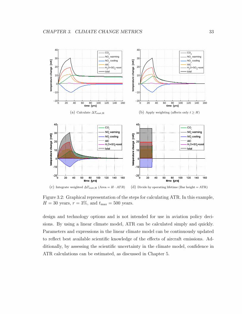
CHAPTER 3. CLIMATE CHANGE METRICS 33
0 20 40 60 80 100 120 140 160−20
−10
0
10
20
30
40
time [yrs]
tem
per
atu
re c
han
ge
[m
K]
CO2
NOx warming
NOx cooling
AICH
2O+SO
4+soot
total
(a) Calculate ∆Tsust,H
0 20 40 60 80 100 120 140 160−20
−10
0
10
20
30
40
time [yrs]
tem
per
atu
re c
han
ge
[m
K]
CO2
NOx warming
NOx cooling
AICH
2O+SO
4+soot
total
(b) Apply weighting (affects only t ≥ H)
(c) Integrate weighted ∆Tsust,H (Area = H ·ATR) (d) Divide by operating lifetime (Bar height = ATR)
Figure 3.2: Graphical representation of the steps for calculating ATR. In this example,H = 30 years, r = 3%, and tmax = 500 years.
design and technology options and is not intended for use in aviation policy deci-
sions. By using a linear climate model, ATR can be calculated simply and quickly.
Parameters and expressions in the linear climate model can be continuously updated
to reflect best available scientific knowledge of the effects of aircraft emissions. Ad-
ditionally, by assessing the scientific uncertainty in the climate model, confidence in
ATR calculations can be estimated, as discussed in Chapter 5.
CHAPTER 3. CLIMATE CHANGE METRICS 34
3.3.3 Alternative Aircraft Design Metrics
Average temperature response is proposed as a climate metric for the application
of aircraft design. However, other metrics could be developed to serve the same
purpose. Each of the considered alternative metrics is based on the same aircraft
emissions scenario of H years of constant emissions followed by zero emissions. The
first is an integrated normalized radiative forcing metric, similar to global warming
potential.[32] This metric, referred to as average radiative forcing response, is defined
as in equation (3.1), where RF replaces ∆T . The weighting function given in equa-
tion (3.2) is applied. The second alternative is an endpoint metric: ∆Tsust(t = H) is
the temperature change after H years of sustained emissions and is similar to global
temperature potential.[32] Aircraft design study results in Ref. [73] demonstrate that
comparisons of climate performance are essentially insensitive to choice of metric be-
tween the options of integrated ∆T , integrated RF, and endpoint ∆T for the specified
emissions scenario. The differences in results with each of these metrics lies primarily
in the weighting of short-lived and long-lived effects which can be adjusted within the
ATR framework using weighting function parameters r and tmax.
Chapter 4
Aircraft Design and Analysis Tools
4.1 Introduction
To explore the design of future aircraft for reduced climate impacts, methods are
needed to assess aircraft performance. Takeoff, climb, cruise, and landing performance
are determined using the conceptual design software PASS, a flexible tool that enables
the integration of new and updated methods. This chapter describes the cost methods
used for economic performance estimation and an updated engine model.
4.2 Program for Aircraft Synthesis Studies
The design of new aircraft encompasses many disciplines including aerodynamics,
structural design, stability and control, and economics. While the final, detailed de-
sign of a new commercial aircraft typically requires several years of work by thousands
of engineers, an initial or conceptual design can be generated quickly using approxi-
mate methods and computational tools. The Program for Aircraft Synthesis Studies
(PASS) is a conceptual design and performance estimation tool containing methods
for each discipline as shown in Figure 4.1.[74] These methods rely on McDonnell Dou-
glas empirical models and newly developed analyses that are described in detail in
Ref. [75]. PASS has been validated and applied in many past aircraft design studies
(e.g., Ref. [7]). When combined with an optimizer, PASS allows for rapid exploration
35

CHAPTER 4. AIRCRAFT DESIGN AND ANALYSIS TOOLS 36
of the design space, including the tradeoffs between economic and environmental per-
formance. A new climate impact module is developed for environmental analysis and
is described in Chapter 5.
Economics
Structures
Stability and Control
Aircraft Performance
Optimizer Climate Impacts
Propulsion
Noise
Aerodynamics
Database
Figure 4.1: Structure of PASS, adapted from Ref. [7].
4.3 Operating Costs
For an aircraft to be economically competitive, its operating costs must be as low as
possible. Total operating costs include both direct and indirect operating costs (DOC
and IOC). Cost effectiveness is often measured by DOC, which includes fuel, crew,
depreciation, insurance, and maintenance costs. The Air Transport Association of
America (ATA) developed a set of equations for computing comparative DOC, and
these methods are applied in PASS.[76] Crew costs are a function of aircraft weight
and flight speed, with larger and slower aircraft having greater crew expenses. Fuel
costs depend not only on mission fuel consumption, but also on the relative price
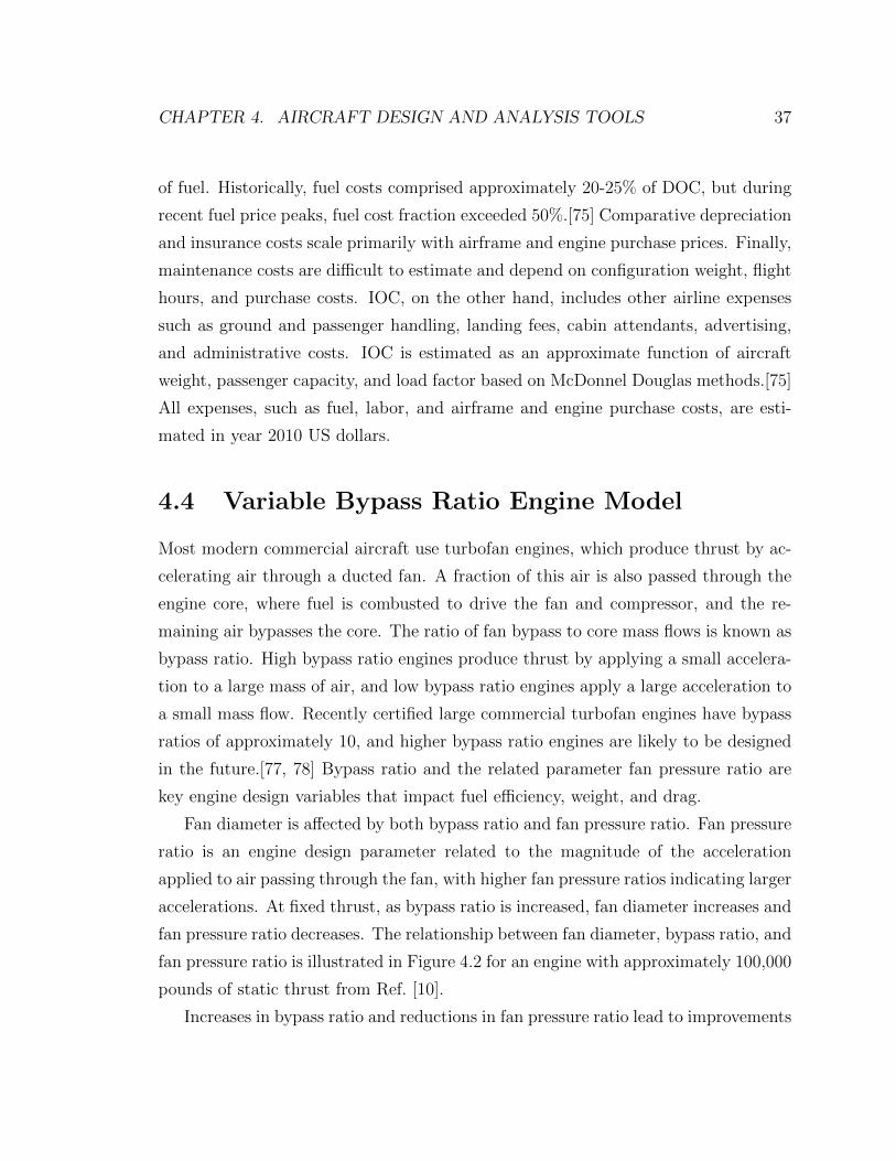
CHAPTER 4. AIRCRAFT DESIGN AND ANALYSIS TOOLS 37
of fuel. Historically, fuel costs comprised approximately 20-25% of DOC, but during
recent fuel price peaks, fuel cost fraction exceeded 50%.[75] Comparative depreciation
and insurance costs scale primarily with airframe and engine purchase prices. Finally,
maintenance costs are difficult to estimate and depend on configuration weight, flight
hours, and purchase costs. IOC, on the other hand, includes other airline expenses
such as ground and passenger handling, landing fees, cabin attendants, advertising,
and administrative costs. IOC is estimated as an approximate function of aircraft
weight, passenger capacity, and load factor based on McDonnel Douglas methods.[75]
All expenses, such as fuel, labor, and airframe and engine purchase costs, are esti-
mated in year 2010 US dollars.
4.4 Variable Bypass Ratio Engine Model
Most modern commercial aircraft use turbofan engines, which produce thrust by ac-
celerating air through a ducted fan. A fraction of this air is also passed through the
engine core, where fuel is combusted to drive the fan and compressor, and the re-
maining air bypasses the core. The ratio of fan bypass to core mass flows is known as
bypass ratio. High bypass ratio engines produce thrust by applying a small accelera-
tion to a large mass of air, and low bypass ratio engines apply a large acceleration to
a small mass flow. Recently certified large commercial turbofan engines have bypass
ratios of approximately 10, and higher bypass ratio engines are likely to be designed
in the future.[77, 78] Bypass ratio and the related parameter fan pressure ratio are
key engine design variables that impact fuel efficiency, weight, and drag.
Fan diameter is affected by both bypass ratio and fan pressure ratio. Fan pressure
ratio is an engine design parameter related to the magnitude of the acceleration
applied to air passing through the fan, with higher fan pressure ratios indicating larger
accelerations. At fixed thrust, as bypass ratio is increased, fan diameter increases and
fan pressure ratio decreases. The relationship between fan diameter, bypass ratio, and
fan pressure ratio is illustrated in Figure 4.2 for an engine with approximately 100,000
pounds of static thrust from Ref. [10].
Increases in bypass ratio and reductions in fan pressure ratio lead to improvements
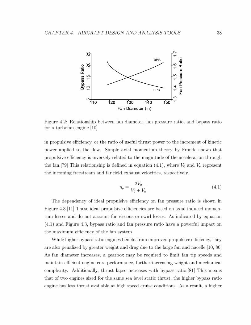
CHAPTER 4. AIRCRAFT DESIGN AND ANALYSIS TOOLS 38
Figure 4.2: Relationship between fan diameter, fan pressure ratio, and bypass ratiofor a turbofan engine.[10]
in propulsive efficiency, or the ratio of useful thrust power to the increment of kinetic
power applied to the flow. Simple axial momentum theory by Froude shows that
propulsive efficiency is inversely related to the magnitude of the acceleration through
the fan.[79] This relationship is defined in equation (4.1), where V0 and Ve represent
the incoming freestream and far field exhaust velocities, respectively.
ηp =2V0
V0 + Ve(4.1)
The dependency of ideal propulsive efficiency on fan pressure ratio is shown in
Figure 4.3.[11] These ideal propulsive efficiencies are based on axial induced momen-
tum losses and do not account for viscous or swirl losses. As indicated by equation
(4.1) and Figure 4.3, bypass ratio and fan pressure ratio have a powerful impact on
the maximum efficiency of the fan system.
While higher bypass ratio engines benefit from improved propulsive efficiency, they
are also penalized by greater weight and drag due to the large fan and nacelle.[10, 80]
As fan diameter increases, a gearbox may be required to limit fan tip speeds and
maintain efficient engine core performance, further increasing weight and mechanical
complexity. Additionally, thrust lapse increases with bypass ratio.[81] This means
that of two engines sized for the same sea level static thrust, the higher bypass ratio
engine has less thrust available at high speed cruise conditions. As a result, a higher
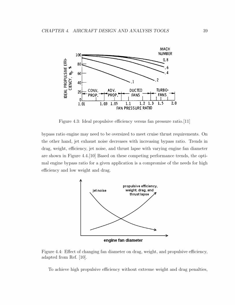
CHAPTER 4. AIRCRAFT DESIGN AND ANALYSIS TOOLS 39
Figure 4.3: Ideal propulsive efficiency versus fan pressure ratio.[11]
bypass ratio engine may need to be oversized to meet cruise thrust requirements. On
the other hand, jet exhaust noise decreases with increasing bypass ratio. Trends in
drag, weight, efficiency, jet noise, and thrust lapse with varying engine fan diameter
are shown in Figure 4.4.[10] Based on these competing performance trends, the opti-
mal engine bypass ratio for a given application is a compromise of the needs for high
efficiency and low weight and drag.
Figure 4.4: Effect of changing fan diameter on drag, weight, and propulsive efficiency,adapted from Ref. [10].
To achieve high propulsive efficiency without extreme weight and drag penalties,

CHAPTER 4. AIRCRAFT DESIGN AND ANALYSIS TOOLS 40
unducted high bypass ratio propfan engines have been considered for application on
large commercial aircraft. NASA funded the Advanced Turboprop Project in the
1980s to explore the benefits of unducted, highspeed aircraft engines.[82, 83, 84] This
project included analyses, wind tunnel testing, and flight tests to demonstrate prop-
fan performance. Traditional unducted turboprop engines are limited to maximum
cruise speeds of Mach 0.65, with significant efficiency losses at higher speeds due to
compressibility. Propfans, on the other hand, employ highly swept, very thin, small
diameter propeller blades designed to operate at speeds of up to Mach 0.8 without
significant compressibility losses.[82] A comparison of the relative fan diameters of
traditional turboprops, propfans, and high bypass ratio turbofans is shown in Figure
4.5.[12]
Figure 4.5: Comparison of fan sizes for turboprop, propfan, and turbofan en-gines (reproduced with permission of the American Institute of Aeronautics andAstronautics).[12]
The combination of high speeds and high efficiencies could enable significant fuel
savings for aircraft driven by propfans. Configuration studies have predicted fuel
burn savings of on the order of 15-30% relative to aircraft with comparable turbofan
technology.[12, 85, 86, 87, 11] However, the Advanced Turboprop Project identified
a number of propfan technical design challenges including noise, aerodynamic and
structural installation issues, blade aeroelastic design, and gearbox design.[85, 86]
For example, without a duct, the cabin interior and propfan blades must be designed
carefully to limit interior and exterior noise to acceptable levels.[88] Recently, there
CHAPTER 4. AIRCRAFT DESIGN AND ANALYSIS TOOLS 41
has been renewed interest by the engine manufacturers in propfan technology owing
to volatile, high fuel prices, and work to resolve these issues continues (e.g., Ref. [89]).
To determine the optimal engine configuration for a particular aircraft application,
engine performance, drag, weight, noise, and cost must be modeled as a function of
bypass ratio. This section describes turbofan and propfan models appropriate for
aircraft conceptual design.
4.4.1 Engine Performance
Engine performance is characterized by specific fuel consumption and maximum avail-
able thrust at varying operating conditions. Performance is modeled by combining an
engine cycle analysis with simple propeller theory. Cycle analysis computes the ther-
modynamic properties of the flow at each station in the engine based on user-specified
design variables and component efficiencies following the methods presented in Refs.
[21, 90]. This approach allows users to quantify the overall performance effects of
changing design parameters such as bypass ratio. The result is a “rubber engine”
that may be scaled up or down in size by adjusting engine mass flow. The same cycle
analysis is applied for both turbofan and propfan engines, and differences between
these configurations are modeled through engine design parameters and efficiencies.
Similar engine cores can be designed to drive ducted or unducted fans with dif-
ferent pressure ratios and numbers of rotors. Efficiency depends on these fan config-
uration design variables. Unducted fans employ either a single rotor or two counter-
rotating propellers. Single rotor propfans benefit from reduced mechanical complex-
ity, but these propellers leave rotational momentum in the propeller wake, leading
to reduced efficiencies. Dual rotor propfans are designed for reduced swirl losses.
Lastly, ducted turbofans are often designed with a rotor and stator to limit swirl
losses and noise. Simple propeller theory is applied to estimate the efficiencies of
different fan configurations, including ducted rotor-stators and unducted single and
dual rotor fans, based on losses from drag and energy left in the wake. The combined
cycle analysis and propeller theory model for turbofan and propfan performance is
described in Appendix A.
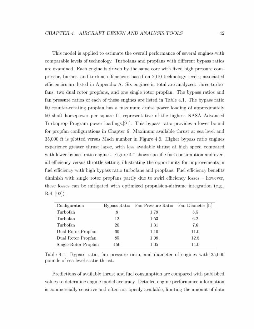
CHAPTER 4. AIRCRAFT DESIGN AND ANALYSIS TOOLS 42
This model is applied to estimate the overall performance of several engines with
comparable levels of technology. Turbofans and propfans with different bypass ratios
are examined. Each engine is driven by the same core with fixed high pressure com-
pressor, burner, and turbine efficiencies based on 2010 technology levels; associated
efficiencies are listed in Appendix A. Six engines in total are analyzed: three turbo-
fans, two dual rotor propfans, and one single rotor propfan. The bypass ratios and
fan pressure ratios of each of these engines are listed in Table 4.1. The bypass ratio
60 counter-rotating propfan has a maximum cruise power loading of approximately
50 shaft horsepower per square ft, representative of the highest NASA Advanced
Turboprop Program power loadings.[91]. This bypass ratio provides a lower bound
for propfan configurations in Chapter 6. Maximum available thrust at sea level and
35,000 ft is plotted versus Mach number in Figure 4.6. Higher bypass ratio engines
experience greater thrust lapse, with less available thrust at high speed compared
with lower bypass ratio engines. Figure 4.7 shows specific fuel consumption and over-
all efficiency versus throttle setting, illustrating the opportunity for improvements in
fuel efficiency with high bypass ratio turbofans and propfans. Fuel efficiency benefits
diminish with single rotor propfans partly due to swirl efficiency losses – however,
these losses can be mitigated with optimized propulsion-airframe integration (e.g.,
Ref. [92]).
Configuration Bypass Ratio Fan Pressure Ratio Fan Diameter [ft]
Turbofan 8 1.79 5.5
Turbofan 12 1.53 6.2
Turbofan 20 1.31 7.6
Dual Rotor Propfan 60 1.10 11.0
Dual Rotor Propfan 85 1.08 12.8
Single Rotor Propfan 150 1.05 14.0
Table 4.1: Bypass ratio, fan pressure ratio, and diameter of engines with 25,000pounds of sea level static thrust.
Predictions of available thrust and fuel consumption are compared with published
values to determine engine model accuracy. Detailed engine performance information
is commercially sensitive and often not openly available, limiting the amount of data

CHAPTER 4. AIRCRAFT DESIGN AND ANALYSIS TOOLS 43
0 0.2 0.4 0.6 0.8 10
0.1
0.2
0.3
0.4
0.5
0.6
0.7
0.8
0.9
1
Mach number
max
inst
alle
d th
rust
/ S
LS in
stal
led
thru
st
sea level
35,000 ft
bpr 8 TFbpr 12 TFbpr 20 TFbpr 60 DRPFbpr 85 DRPFbpr 150 SRPF
Figure 4.6: Maximum available thrust versus Mach number at varying altitude forturbofans and dual and single rotor propfans of varying bypass ratio.
available to validate this model. Figure 4.8 compares model predictions of available
thrust and specific fuel consumption with performance estimates for a NASA study
high bypass ratio geared turbofan.[13] Predictions of maximum available thrust and
specific fuel consumption agree over a wide range of speeds and altitudes.
Fuel consumption estimates also concur with performance data published by
NASA for a bypass ratio 7 turbofan and a highly loaded propfan at Mach 0.7 and
30,000 ft altitude.[87] Both the described model and the NASA reference predict spe-
cific fuel consumptions of 0.43 and 0.55 hr−1 at maximum throttle. These model re-
sults also correspond well to NASA estimates for specific fuel consumption of a bypass
ratio 8 turbofan of approximately 0.57 hr−1 at Mach 0.8 and 30,000 ft altitude.[93]
Furthermore, results generally follow predictions by engine manufacturers of fuel con-
sumption savings on the order of 15% by propfans relative to advanced turbofans.[89]

CHAPTER 4. AIRCRAFT DESIGN AND ANALYSIS TOOLS 44
0.3 0.4 0.5 0.6 0.7 0.8 0.9 10.38
0.4
0.42
0.44
0.46
0.48
0.5
0.52
0.54
0.56
0.58
thrust / max available thrust
inst
alle
d sf
c [
1/hr
]
bpr 8 TFbpr 12 TFbpr 20 TFbpr 60 DRPFbpr 85 DRPFbpr 150 SRPF 0.5
0.48
0.46
0.44
0.42
0.4
0.38
0.36
0.34
inst
alle
d ov
eral
l effi
cien
cy
Mach 0.8, 35,000 ft altitude
Figure 4.7: Installed specific fuel consumption and overall efficiency versus throttlesetting for turbofans and propfans of varying bypass ratio.
4.4.2 Engine Geometry
To estimate engine weight and drag, dimensions must be known. Section 4.4.1 and
Appendix A describe a model for a rubberized, dimensionless engine. Once thrust is
specified at a given operating condition, the engine can be sized, including determi-
nation of fan diameter and engine length.
Turbofan diffusers and fans are designed to achieve a specified fan capacity. The
diffuser decelerates incoming air, and modern turbofan engines are generally designed
with fan capacities corresponding to maximum fan face Mach numbers of approxi-
mately 0.66 at top of climb.[94] The top of climb condition for engines in this study
is Mach 0.80, 35,000 ft altitude. Based on the specified fan face Mach number, the
fan area and diameter, Afan and Dfan, can be estimated from equations (4.2) and
(4.3). In these equations, the subscript toc refers to top of climb conditions, TT2 and
PT2 are fan face stagnation temperature and pressure, Mfan is the maximum fan face
Mach number, and ξ is the fan hub-to-tip ratio. The function MFP is the mass flow

CHAPTER 4. AIRCRAFT DESIGN AND ANALYSIS TOOLS 45
0 0.2 0.4 0.6 0.8 10
5,000
10,000
15,000
20,000
25,000
30,000
Mach number
avai
labl
e th
rust
[lb
]
sea level
10,000 ft
25,000 ft
35,000 ft
43,000 ft
bpr 10 TFbpr 14 TFNASA UHB GTF
(a)
0 2000 4000 6000 8000 10000 120000.4
0.45
0.5
0.55
0.6
0.65
thrust [lb]
spec
ific
fuel
con
sum
ptio
n [
1/hr
]
M=0.8, 35,000 ft
M=0.6, 20,000 ft
bpr 10 TFbpr 14 TFNASA UHB GTF
(b)
Figure 4.8: Comparison of available thrust and specific fuel consumption for highbypass ratio engines, from model predictions and a NASA study.[13]
function defined in Ref. [21].
Afan =m0,toc
√TT2,toc
PT2,tocMFP (Mfan)(4.2)
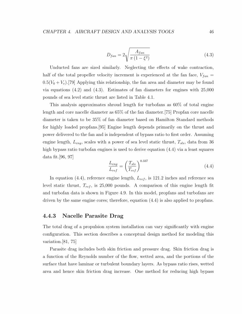
CHAPTER 4. AIRCRAFT DESIGN AND ANALYSIS TOOLS 46
Dfan = 2
√Afan
π (1− ξ2)(4.3)
Unducted fans are sized similarly. Neglecting the effects of wake contraction,
half of the total propeller velocity increment is experienced at the fan face, Vfan =
0.5(V0 + Ve).[79] Applying this relationship, the fan area and diameter may be found
via equations (4.2) and (4.3). Estimates of fan diameters for engines with 25,000
pounds of sea level static thrust are listed in Table 4.1.
This analysis approximates shroud length for turbofans as 60% of total engine
length and core nacelle diameter as 65% of the fan diameter.[75] Propfan core nacelle
diameter is taken to be 35% of fan diameter based on Hamilton Standard methods
for highly loaded propfans.[95] Engine length depends primarily on the thrust and
power delivered to the fan and is independent of bypass ratio to first order. Assuming
engine length, Leng, scales with a power of sea level static thrust, Tsls, data from 36
high bypass ratio turbofan engines is used to derive equation (4.4) via a least squares
data fit.[96, 97]
LengLref
=
(TslsTref
)0.337
(4.4)
In equation (4.4), reference engine length, Lref , is 121.2 inches and reference sea
level static thrust, Tref , is 25,000 pounds. A comparison of this engine length fit
and turbofan data is shown in Figure 4.9. In this model, propfans and turbofans are
driven by the same engine cores; therefore, equation (4.4) is also applied to propfans.
4.4.3 Nacelle Parasite Drag
The total drag of a propulsion system installation can vary significantly with engine
configuration. This section describes a conceptual design method for modeling this
variation.[81, 75]
Parasite drag includes both skin friction and pressure drag. Skin friction drag is
a function of the Reynolds number of the flow, wetted area, and the portions of the
surface that have laminar or turbulent boundary layers. As bypass ratio rises, wetted
area and hence skin friction drag increase. One method for reducing high bypass
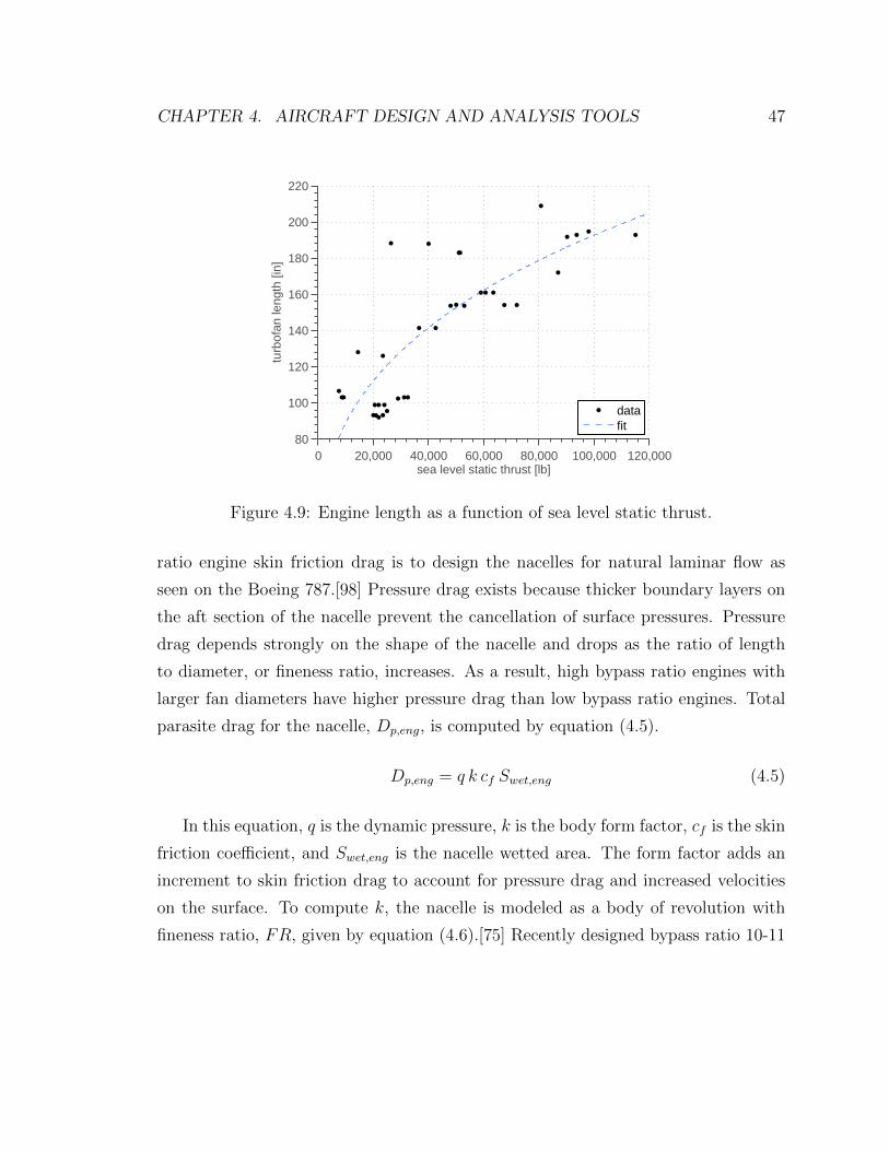
CHAPTER 4. AIRCRAFT DESIGN AND ANALYSIS TOOLS 47
0 20,000 40,000 60,000 80,000 100,000 120,00080
100
120
140
160
180
200
220
sea level static thrust [lb]
turb
ofan
leng
th [i
n]
datafit
Figure 4.9: Engine length as a function of sea level static thrust.
ratio engine skin friction drag is to design the nacelles for natural laminar flow as
seen on the Boeing 787.[98] Pressure drag exists because thicker boundary layers on
the aft section of the nacelle prevent the cancellation of surface pressures. Pressure
drag depends strongly on the shape of the nacelle and drops as the ratio of length
to diameter, or fineness ratio, increases. As a result, high bypass ratio engines with
larger fan diameters have higher pressure drag than low bypass ratio engines. Total
parasite drag for the nacelle, Dp,eng, is computed by equation (4.5).
Dp,eng = q k cf Swet,eng (4.5)
In this equation, q is the dynamic pressure, k is the body form factor, cf is the skin
friction coefficient, and Swet,eng is the nacelle wetted area. The form factor adds an
increment to skin friction drag to account for pressure drag and increased velocities
on the surface. To compute k, the nacelle is modeled as a body of revolution with
fineness ratio, FR, given by equation (4.6).[75] Recently designed bypass ratio 10-11

CHAPTER 4. AIRCRAFT DESIGN AND ANALYSIS TOOLS 48
Trent 1000 and GEnx engines have fineness ratios of approximately 2.5.
FR ≈ Leng +Dinlet
0.9Dinlet
(4.6)
Inlet diameter, Dinlet, is taken to be 1.1Dfan for turbofans and 0.35Dfan for prop-
fans. Form factor is determined from fineness ratio using Figure 4.10. Data in the
figure for fineness ratios of 4 to 10 is based on Ref. [81]. Form factors for lower fineness
ratios are computed following Ref. [75] by relating drag to surface velocity increases
on ellipsoids of varying fineness.
1 2 3 4 5 6 7 81
1.5
2
2.5
3
3.5
4
4.5
fineness ratio
nace
lle fo
rm fa
ctor
k ≈ 1.0706 + 2.0306 e−0.5228 FR + 17.9547 e−2.3116 FR
curve fitdata
Figure 4.10: Nacelle form factor versus fineness ratio.
The skin friction coefficient is computed for the freestream Mach number and flow
Reynolds number based on nacelle length and specified boundary layer transition
location. Wetted area is computed based on nacelle dimensions in equation (4.7). For
turbofans, the forward nacelle diameter is 1.1Dfan and the aft diameter is 0.65Dfan.
For propfans, the nacelle diameter is a constant 0.35Dfan.
Swet,eng =
[0.6 π (1.1Dfan) + 0.4 π (0.65Dfan)] Leng for turbofans
π (0.35Dfan)Leng for propfans(4.7)

CHAPTER 4. AIRCRAFT DESIGN AND ANALYSIS TOOLS 49
Finally, total nacelle parasite drag may be computed for any operating condition
via equation (4.5).
4.4.4 Weight Estimation
An engine weight model is developed to capture the variation in propulsion system
weight with changes to bypass ratio and thrust. Separate weight models are presented
for ducted turbofan and unducted single and dual rotor propfan engines.
First, the dry engine weight of a ducted turbofan engine is considered. It is
assumed that dry turbofan weight can be separated into contributions from the engine
core and fan. The weight of the engine core is expected to depend primarily on
thrust. In this model, core weight is a linear function of sea level static thrust and is
independent of bypass ratio. Fan weight, on the other hand, depends on bypass ratio.
If the fan was a solid disk, then based on volume considerations fan weight would scale
with diameter squared. If the fan was a constant-chord propeller, then fan weight
would scale linearly with diameter. In reality, the total volume of a typical engine
fan is somewhere between a solid disk and a constant-chord propeller; therefore, fan
weight is expected to scale with fan diameter to a power between one and two.
Data from 36 modern high bypass turbofans is used to fit equation (4.8) for dry
turbofan weight, Wtf,dry.[96, 97] By minimizing the root-mean-square weight error,
values for the constants are found. Reference engine weight, Wref , is 10,000 pounds
and reference engine diameter, Dref , is 8 ft. A comparison of predicted and actual
weight for the 36 current engines is shown in Figure 4.11. Two plots are shown
because two independent parameters, sea level static thrust and fan diameter, are
used in the engine weight fit. (Note: Several separate engines use fans with equal
diameters, as indicated in Figure 4.11(b).)
Wtf,dry
Wref
= 0.098TslsWref
+ 0.452
(Dfan
Dref
)1.68
(4.8)
The propfan weight model is divided into core, fan, and gearbox weight elements,
as given by equation (4.9). In this model, identical cores drive turbofans and propfans,

CHAPTER 4. AIRCRAFT DESIGN AND ANALYSIS TOOLS 50
0 20,000 40,000 60,000 80,000 100,000 120,0000
4,000
8,000
12,000
16,000
20,000
sea level static thrust [lb]
turb
ofan
dry
wei
ght [
lb]
datafit
(a)
3 4 5 6 7 8 9 10 110
4,000
8,000
12,000
16,000
20,000
fan diameter [ft]
turb
ofan
dry
wei
ght [
lb]
datafit
(b)
Figure 4.11: Variation in turbofan weight with sea level static thrust and fan diameter.
so the same core weight model is applied to both engine types. The fan weight model
depends on fan diameter and disk loading and is based on a Hamilton Standard
method.[99] Their method developed for single rotor configurations with 800 ft/sec

CHAPTER 4. AIRCRAFT DESIGN AND ANALYSIS TOOLS 51
tip speed and includes the weight of the fan blades, pitch change mechanism, hub,
deicing, and spinner. It is assumed that this method can be extended to dual rotation
propellers by scaling the model by the number of rotors, Nrot. Lastly, gearbox weight
is also based on a Hamilton Standard method.[95] Gearbox weight is proportional to
maximum output torque, which for fans with fixed tip speed is directly related to the
product of fan diameter and power to the fan, Psls. In this equation, reference fan
power, Pref , is 5,000 horsepower, and Dref and Wref are defined as in equation (4.8).
Gearbox weight also scales with the square root of gear ratio, GR, defined as the ratio
of fan and low pressure turbine rotational rates. Gear ratio is computed assuming a
maximum propfan tip speed of 800 ft/sec and a design low pressure turbine rotational
rate of 800 rad/sec.[21]
Wpf,dry = Wpf,core +Wpf,fan +Wpf,gearbox
Wpf,dry
Wref
= 0.098TslsWref
+ 0.059Nrot
(PslsPref
)0.3(Dfan
Dref
)1.836
+ 0.021PslsPref
Dfan
Dref
√GR
8
(4.9)
Turbofan and propfan weights are compared in Figure 4.12 for engines sized to
produce 25,000 pounds of sea level static thrust. In the figure, turbofan bypass ratios
range from 5 to 20, dual rotor propfans from 60 to 110, and single rotor propfans from
90 to 200. Dual rotor propfans are heavier than moderate bypass ratio turbofans due
to their larger rotor diameters and the presence of a gearbox. However, propfans do
offer a lighter weight alternative to very high bypass ratio turbofans. Because the
turbofan weight model is based on existing conventional engines, there is no explicit
modeling of the gearbox and/or the additional low pressure turbine stages that would
be necessary for very large fans. Allowable fan tip speeds for turbofans are almost
double those of propfans, and thus turbofans do not require as large of a gearbox
as a propfans with equal rotor diameters. Nonetheless, weight is underestimated for
turbofans with very large diameter rotors.
Finally, equations (4.8) and (4.9) estimate dry engine weight. Total propulsion
system weight includes the nacelle and pylon, controls, lubrication, and fuel systems.

CHAPTER 4. AIRCRAFT DESIGN AND ANALYSIS TOOLS 52
4 6 8 10 12 14 164000
4500
5000
5500
6000
6500
7000
7500
fan diameter [ft]
engi
ne d
ry w
eigh
t [l
b]
turbofanSR propfanDR propfan
Figure 4.12: Turbofan and single and dual rotor propfan dry weight versus fan diam-eter for 25,000 sea level static thrust engines.
Turbofan propulsion system weight is approximately 60% greater than dry weight
alone.[75] Propfan propulsion system weight is approximately 30% greater than dry
weight alone.[95] The turbofan model is based on data for engines designed and cer-
tified over the last several decades, and the propfan model is based on late 1980s
technology. For engines with entry-into-service of 2010 or later, lighter weight mate-
rials and improved design may enable weight reductions.
4.4.5 Certification Noise
Newly certified aircraft are required to meet standards for maximum community noise
during takeoff and landing. In addition, a growing number of airports have estab-
lished individual noise restrictions, curfews, and charges.[100] To allow for operational
flexibility and economic competitiveness, future aircraft will likely need to be quieter
than today’s aircraft. A large fraction of total noise during both takeoff and ap-
proach is produced by the engines.[7] This noise varies depending on bypass ratio and
whether the fan is ducted or unducted. This section describes a model for estimating
the certification noise of different engine configurations.

CHAPTER 4. AIRCRAFT DESIGN AND ANALYSIS TOOLS 53
Current ICAO Chapter 4 regulations restrict noise measured at approach, flyover,
and sideline conditions. Certification noise is computed using the methodology de-
scribed in Ref. [75]. In this model, total noise at each condition is estimated based
on measured noise at a specified distance from a bypass ratio 6 reference turbofan
engine. This noise is scaled for an individual aircraft configuration based on the size
and number of engines, engine throttle setting, and the distance between the aircraft
and the regulated noise measurement location. At approach conditions, an estimate
of airframe noise is added.[75] Increases in bypass ratio affect takeoff engine noise,
resulting in lower jet noise but greater fan noise. Moderately high bypass ratio turbo-
fans are expected to be quieter than current engines, and a number of studies predict
noise savings for engines with bypass ratios of up to 15.[7, 101, 102] Analysis of ICAO
certification data reveals an approximate reduction of 1.5 dB at sideline and 0.5 dB
at flyover per unit increase in bypass ratio.[103] However, also included in this trend
are improved acoustic technologies, including advanced duct liners. Following results
published by Antoine, turbofan sideline and flyover noise are assumed to reduce by
0.7 dB and 0.5 dB, respectively, per unit increase in bypass ratio.[7] Additionally, the
reference engine noise is reduced by 5 dB at all conditions to account for improved
technology.[75]
Propfan engines lack a shroud to protect surroundings from fan noise. Meeting
current Chapter 4 and future, more restrictive regulations poses a challenge for prop-
fan aircraft. A recent workshop cites the general expectation from industry that
propfan aircraft can meet Chapter 4 targets with a margin, but steeper climb and
approach paths may be required to reduce noise exposure.[104, 105] In this research,
the reference turbofan noise is shifted to match certification noise predictions based
on scale model tests by Hoff et al.[106] Based on this data, counter-rotating propfan
engines are approximately 0.5 dB quieter than the reference engine at each condi-
tion. Counter-rotating propfans are noisier than single rotor propfans due to rear
rotor wake aerodynamic interactions and out-of-phase acoustic interactions.[107, 108]
Single rotor engines are modeled to be 2.5 dB quieter than counter-rotating propfans

CHAPTER 4. AIRCRAFT DESIGN AND ANALYSIS TOOLS 54
at each noise measurement condition. This estimate is based on single and dual ro-
tor porpfan comparative noise measurements, demonstrating that single rotors are at
least 2.5 dB quieter at each blade harmonic frequency.[108]
4.4.6 Engine Maintenance and Acquisition Costs
Engine costs are incurred both initially for the purchase of the aircraft and during
operation for maintenance. The availability of engine acquisition cost data is very
limited, particularly for advanced high bypass ratio turbofans and propfans. Turbo-
fan acquisition costs are estimated using the data in Ref. [109]. An empirical method
relates cost to sea level static thrust per engine based on engines certified and pro-
duced prior to 1975. Because very high bypass ratio turbofans have large, heavy
fans, this method is expected to underpredict acquisition costs for high bypass ratio
engines. Pratt and Whitney and Hamilton Standard estimate the acquisition costs
of a turbofan and propfan designed for the same application to be within 1% of one
another.[93] Based on this finding, it is assumed that propfan acquisition costs can
be computed with the turbofan cost model.
Turbofan maintenance costs are computed with the ATA direct operating costs
method.[76] Maintenance costs include both labor and parts costs and are a function
of flight time and sea level static thrust. Similar to acquisition costs, preliminary
estimates of propfan maintenance costs yield rates that are within ±8% of turbofan
rates. This result is supported by a NASA study presenting comparable maintenance
costs for advanced turbofan and propfan engines.[110] Therefore, propfan mainte-
nance costs are assumed to scale similarly to turbofan costs.

Chapter 5
Linear Climate Model with
Altitude Variation
5.1 Introduction
Climate impacts from aircraft operations can be estimated based on the quantity and
location of released emissions and knowledge about the climate system. Emissions of
CO2, H2O, NOx, soot, and sulfate particles each affect the climate system as described
in Chapter 2. The first section of this chapter describes methods for quantifying an
aircraft’s total emissions based on estimate of aircraft and engine performance. The
second part of this chapter presents a climate model that translates aircraft emissions
into radiative forcing and temperature change. The limitations of this climate model
and a method for quantifying uncertainty in impact estimates are also discussed.
Climate models range in sophistication from simple linear temperature response
models to complex three-dimensional global climate models. Although linear models
are less accurate than more complex models, they enable quick estimation of impacts
and have been applied to several aviation emissions studies.[53, 47, 68, 56, 55, 1,
32] Linear climate models developed for aviation studies compute the impacts from
emissions deposited directly into the upper troposphere and lower stratosphere, which
can lead to different climate impacts compared with ground-based emissions from
other sectors. These climate models greatly simplify the physics and chemistry of
55
CHAPTER 5. LINEAR CLIMATE MODEL WITH ALTITUDE VARIATION 56
aircraft induced climate change, and the analysis generated by these models captures
only first order effects; however, their speed makes linear models appropriately suited
for quantifying the various tradeoffs in aircraft conceptual design. The climate model
developed for this study distinguishes itself from many other linear climate models
through its inclusion of altitude variation for NOx and AIC radiative forcings.
5.2 Emissions
The first step in assessing the climate impacts of a particular aircraft is to construct
a scenario of future emissions produced by that aircraft. This emissions trajectory
is computed by assuming the aircraft flies its typical mission a specified number of
times per year. Utilization rate, U(t), refers to the number of missions flown in year,
and emissions per flight, ei, refers to the total quantity of species i released during
the typical mission. Annual emissions of each species, Ei(t), may be estimated with
equation (5.1).
Ei(t) = ei U(t) (5.1)
Emissions per flight are related to fuel consumption through the emissions index
(EI), or the mass ratio of emitted species to fuel burned, as shown in equation (5.2).
The emissions index for each species i is assumed to be piecewise constant, with a
value of EIi,j during the jth mission segment.
ei =∑
mission
EIi,jWfuel,j (5.2)
Thus, for a given aircraft utilization rate, overall emissions savings can be achieved
via reductions in either fuel burn or emissions index. Mission fuel consumption during
the jth flight segment, Wfuel,j, is calculated using the aircraft and engine performance
tools described in Chapter 4. Emissions index, EIi, is a key parameter determining
the overall mass of emissions. For many species, EI is a property of the fuel and
cannot be changed; however, EINOx is a performance parameter that can be adjusted
via design.

CHAPTER 5. LINEAR CLIMATE MODEL WITH ALTITUDE VARIATION 57
5.2.1 Carbon Dioxide, Water Vapor, Soot, and Sulfate Emis-
sions Indices
The EIs of CO2, H2O, and SO4 are solely dependent on the composition of the fuel
and taken to be constants.[3] Sulfate emissions index is derived from average fuel
sulfur content and a 50% conversion factor of fuel sulfur into optically active sulfate,
following the IPCC.[3] As noted in Chapter 2, soot emissions index can vary with
engine operating condition, but because soot comprises a small fraction of total cli-
mate impacts (on the order of less than 5%, e.g., Ref. [29]), this factor can also be
assumed constant without significant loss in accuracy for many studies of interest.
These EIs are listed in Table 5.1. Because these emissions indices are constant, the
summation given in equation (5.2) is simply the product of EIi and total mission fuel
consumption.
Species Emissions Index
CO2 3.16 kg CO2kg fuel
H2O 1.26 kg H2Okg fuel
SO4 2.0e-4 kg Skg fuel
soot 4.0e-5 kg sootkg fuel
Table 5.1: Emissions indices.[3]
5.2.2 Nitrogen Oxide Emissions Index
Unlike emissions indices for CO2 and other species, NOx emissions index is not con-
stant and varies with engine throttle setting, flight speed, and altitude. The variation
in emissions index with operating condition and combustor design is complex to model
analytically, but different empirical correlation methods exist to approximately de-
scribe the relationship between combustor parameters and EINOx . P3-T3 methods
model emissions index as a function of combustor inlet temperature and pressure,
ambient conditions, and sometimes other combustor design parameters. The P3-T3
method is the industry standard for computing NOx emissions and is very accurate:

CHAPTER 5. LINEAR CLIMATE MODEL WITH ALTITUDE VARIATION 58
applying a P3-T3 correlation to the combustor for which it was derived enables emis-
sions index prediction at flight conditions to within 5-10%.[40, 46, 45, 3] However,
P3-T3 correlations lose accuracy when applied more generally and are not appropriate
for studying changes to combustor design.[39]
Fuel flow correlation methods are also used to model NOx cruise emissions in-
dex based on ICAO landing and takeoff certification emissions measurements.[42, 41]
These methods are less accurate than P3-T3 correlations but are useful in stud-
ies where combustor inlet temperature and pressure data is unavailable (e.g., Refs.
[43, 44, 8, 45, 46]). In this research, combustor temperature and pressure are mod-
eled directly as described in Chapter 4 and Appendix A, hence P3-T3 methods are
preferred.
Lefebvre developed a NOx emissions P3-T3 correlation based on the assumption
that emissions index is proportional to the product of mean residence time in the
combustion zone, chemical reaction rate, and mixing rate.[40] Residence time depends
on combustor length and flow velocity, L and V . Reaction rate is a function of
combustor temperature and pressure, T and P , with higher NOx formation rates at
higher temperatures and pressures. Mixing rate is assumed to be a function of the
pressure drop through the combustor, ∆P , but this emissions index dependence is
often found to be very weak.[40] Lefebvre’s model for emissions index is given in
equation (5.3).
EINOx ∝ residence time · reaction rate ·mixing rate
= A · LV· Pm exp (zT ) ·
(∆P
P
)n(5.3)
Correlations of this form have been derived for several different combustors.[39,
111, 30, 112, 113] Values of constants A, z, m, and n are found through regres-
sion analysis of emissions data from extensive combustor rig or full scale engine
tests and consideration of chemical timescales.[111] Most combustors demonstrate
dependence on combustor inlet pressure to a power, m, between 0.4 to 0.6.[111] In
many fixed design correlations, dependence on varying flow velocity and liner pressure
drop are neglected, leaving dependence on combustor pressure and temperature only.

CHAPTER 5. LINEAR CLIMATE MODEL WITH ALTITUDE VARIATION 59
This research applies the EINOx correlation shown in equation (5.4), developed for
the dual annular combustor studied during NASA’s Experimental Clean Combustor
Program.[113] This correlation is expected to approximately model the performance
of the GE90-85B dual annular combustor, which is representative of modern high
bypass ratio, high overall pressure ratio turbofan performance.[111]
EINOx = 0.0986
(PT3
101325
)0.4
exp
(TT3
194.4− H0
53.2
)(5.4)
In the above equation, pressure is measured in Pascals, temperature in Kelvin,
and specific humidity, H0, in grams of water per kilogram of dry air. Following
Baughcum et al., specific humidity is calculated as a function of altitude assuming
60% relative humidity.[43] This emissions correlation is also consistent with the IPCC
P3-T3 method, which suggests relating sea level static and cruise emissions indices at
the same TT3 by scaling with PT30.4 and correcting for differences in humidity.[8, 45, 3]
It should be noted that the correlation in equation (5.4) was derived for a dual
annular combustor with lower core temperatures and pressures than those observed on
newly certified engines with overall pressure ratios of 50 and higher.[96] This reduces
the accuracy of emissions index predictions; however, correlations for newer engines
are proprietary and not publicly available. Emission rates of more advanced low NOx
combustors are modeled by applying a scaling factor to equation (5.4), which will be
described in technology studies in Chapter 6.
Figure 5.1 shows emissions index predictions for a bypass ratio 8 turbofan with a
sea level static overall pressure ratio of 41. Emissions index is plotted versus throt-
tle setting for both sea level static and cruise conditions. This engine meets ICAO
CAEP6 landing and takeoff emissions standards due to its relatively low fuel con-
sumption despite having very high full throttle emissions indices. At cruise, engine
core temperatures and therefore emissions index decrease with reduced thrust set-
ting and cruise speed. Emissions index is primarily a function of engine core design,
and therefore engines with different bypass ratios but the similar cores exhibit nearly
identical variation in EI with throttle.
The total mass of NOx emissions for a single mission is computed via equation (5.2)
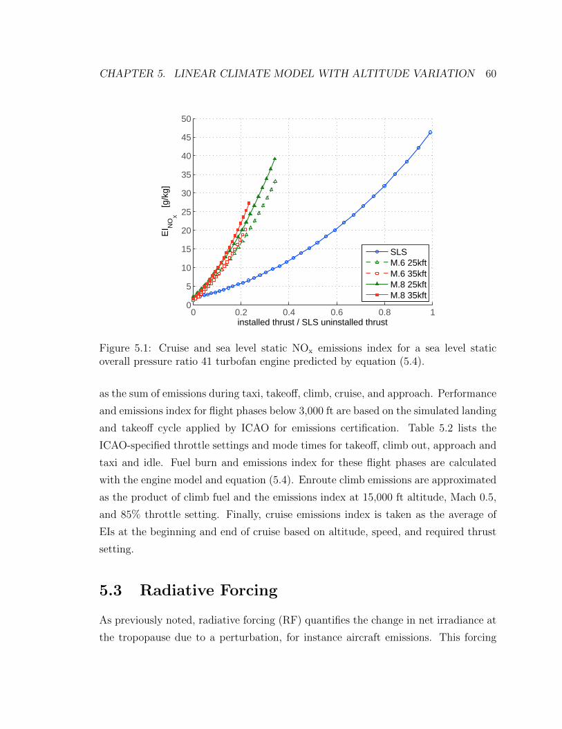
CHAPTER 5. LINEAR CLIMATE MODEL WITH ALTITUDE VARIATION 60
0 0.2 0.4 0.6 0.8 10
5
10
15
20
25
30
35
40
45
50
installed thrust / SLS uninstalled thrust
EI N
OX
[g
/kg]
SLSM.6 25kftM.6 35kftM.8 25kftM.8 35kft
Figure 5.1: Cruise and sea level static NOx emissions index for a sea level staticoverall pressure ratio 41 turbofan engine predicted by equation (5.4).
as the sum of emissions during taxi, takeoff, climb, cruise, and approach. Performance
and emissions index for flight phases below 3,000 ft are based on the simulated landing
and takeoff cycle applied by ICAO for emissions certification. Table 5.2 lists the
ICAO-specified throttle settings and mode times for takeoff, climb out, approach and
taxi and idle. Fuel burn and emissions index for these flight phases are calculated
with the engine model and equation (5.4). Enroute climb emissions are approximated
as the product of climb fuel and the emissions index at 15,000 ft altitude, Mach 0.5,
and 85% throttle setting. Finally, cruise emissions index is taken as the average of
EIs at the beginning and end of cruise based on altitude, speed, and required thrust
setting.
5.3 Radiative Forcing
As previously noted, radiative forcing (RF) quantifies the change in net irradiance at
the tropopause due to a perturbation, for instance aircraft emissions. This forcing

CHAPTER 5. LINEAR CLIMATE MODEL WITH ALTITUDE VARIATION 61
Mode Time in Mode [mins] Thrust Setting
Takeoff 0.7 100%
Climb out 2.2 85%
Approach 4.0 30%
Taxi and Idle 26.0 7%
Table 5.2: ICAO emissions certification simulated landing and takeoff cycle.[3]
measures the magnitude of a climate impact and is linearly related to the change
in global mean equilibrium surface temperature. Radiative forcing causes a climate
system response, which may include changes in surface temperature, precipitation,
extreme weather events, and other climate properties.[6] Positive radiative forcing
induces warming, and negative forcing causes cooling.
This section provides methods for computing time-varying radiative forcing as a
function of altitude and mass of aircraft emissions. Different models are required
for long-lived gases, short-lived pollutants, and aviation induced cloudiness. The
parameters used in this model are based on current best estimates, and many of
these parameters are associated with large uncertainty. Probability distributions for
each parameter are listed, and a method for aggregating climate model uncertainty
is discussed later in this chapter.
5.3.1 Altitude Variation
Radiatively active aircraft emissions differ from ground source emissions because they
are deposited directly into the upper troposphere and lower stratosphere. In partic-
ular, the magnitude of effects from NOx emissions and aviation induced cloudiness
vary significantly depending on emissions altitude. To account for this variation,
altitude-dependent forcing factors are developed. NOx forcing factors are unitless pa-
rameters that represent the radiative forcing per emission at a particular altitude, h,
normalized by fleetwide average radiative forcing per NOx emissions. Similarly, AIC
forcing factors are defined as the RF per distance flown at an altitude, h, normalized
by fleetwide average AIC forcing per distance flown. These functions, si(h), are based
on data from perturbational aircraft emissions studies by Kohler et al. and Radel and
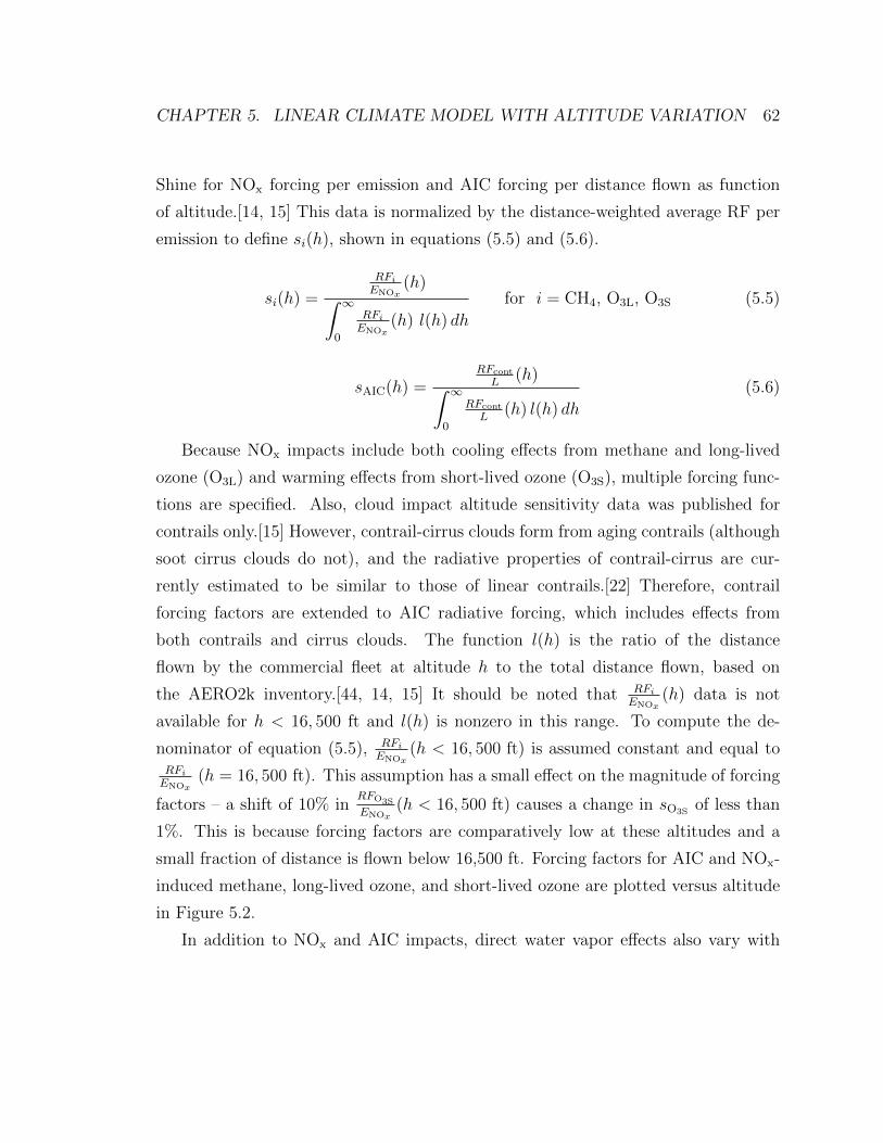
CHAPTER 5. LINEAR CLIMATE MODEL WITH ALTITUDE VARIATION 62
Shine for NOx forcing per emission and AIC forcing per distance flown as function
of altitude.[14, 15] This data is normalized by the distance-weighted average RF per
emission to define si(h), shown in equations (5.5) and (5.6).
si(h) =
RFiENOx
(h)∫ ∞0
RFiENOx
(h) l(h) dh
for i = CH4, O3L, O3S (5.5)
sAIC(h) =RFcont
L(h)∫ ∞
0
RFcont
L(h) l(h) dh
(5.6)
Because NOx impacts include both cooling effects from methane and long-lived
ozone (O3L) and warming effects from short-lived ozone (O3S), multiple forcing func-
tions are specified. Also, cloud impact altitude sensitivity data was published for
contrails only.[15] However, contrail-cirrus clouds form from aging contrails (although
soot cirrus clouds do not), and the radiative properties of contrail-cirrus are cur-
rently estimated to be similar to those of linear contrails.[22] Therefore, contrail
forcing factors are extended to AIC radiative forcing, which includes effects from
both contrails and cirrus clouds. The function l(h) is the ratio of the distance
flown by the commercial fleet at altitude h to the total distance flown, based on
the AERO2k inventory.[44, 14, 15] It should be noted that RFiENOx
(h) data is not
available for h < 16, 500 ft and l(h) is nonzero in this range. To compute the de-
nominator of equation (5.5), RFiENOx
(h < 16, 500 ft) is assumed constant and equal toRFiENOx
(h = 16, 500 ft). This assumption has a small effect on the magnitude of forcing
factors – a shift of 10% inRFO3S
ENOx(h < 16, 500 ft) causes a change in sO3S
of less than
1%. This is because forcing factors are comparatively low at these altitudes and a
small fraction of distance is flown below 16,500 ft. Forcing factors for AIC and NOx-
induced methane, long-lived ozone, and short-lived ozone are plotted versus altitude
in Figure 5.2.
In addition to NOx and AIC impacts, direct water vapor effects also vary with

CHAPTER 5. LINEAR CLIMATE MODEL WITH ALTITUDE VARIATION 63
0 0.25 0.5 0.75 1.0 1.25 1.5 1.75 2.016,000
20,000
24,000
28,000
32,000
36,000
40,000
44,000
forcing factor s
alti
tud
e h
[ft
]
O3S
CH4 & O
3L
AIC
Figure 5.2: Radiative forcing factor data for NOx impacts and aviation induced cloudi-ness, based on results from Refs. [14] and [15].
emission altitude. In the range of altitudes subsonic aircraft typically cruise (30,000-
40,000 ft), nearly all water vapor is emitted into the troposphere or lowermost strato-
sphere where it has a very short residence time determined by the hydrological cycle
and a weak impact on climate.[3] However, at higher altitudes, a greater quantity
of emissions are released into the dry stratosphere, where water vapor has a longer
residence time and therefore a more significant impact. At altitudes of approximately
60,000 ft, water vapor emissions have potent climate impacts, causing concern for a
future supersonic aircraft fleet.[3] A study of subsonic aircraft altitude shifts rang-
ing from -6000 ft to +2000 ft shows trend of increasing H2O forcing with increasing
altitude.[114] However, because the net impacts of H2O are small over the range of
subsonic altitudes compared with CO2, NOx, and AIC impacts, this variation can be
neglected.

CHAPTER 5. LINEAR CLIMATE MODEL WITH ALTITUDE VARIATION 64
5.3.2 Carbon Dioxide
Carbon dioxide is a well-mixed greenhouse gas with a long lifetime relative to chemical
processes in the atmosphere. Because of this, aviation CO2 impacts do not vary
with altitude can be treated in the same manner as all other anthropogenic CO2
sources. The IPCC estimates the radiative forcing caused by small perturbational
emissions of CO2 with equations (5.7) and (5.8).[4] This linear model is based on the
assumption of constant background CO2 concentrations of 378 parts per million by
volume (ppmv). This is an unlikely trajectory in the near-term, and the impact of
this scenario uncertainty is addressed later.
RFCO2(t) =
∫ t
0
GCO2(t− τ)ECO2(τ) dτ (5.7)
GCO2(t) = ACO2
[1 +
3∑j=1
αcj
(exp
(−tτcj
)− 1
)](5.8)
In these equations, the expression GCO2(t) represents the decay of radiative forcing
caused by a pulse emission of CO2, measured in W/m2 per kg CO2. The bracketed
portion of equation (5.8) describes the fraction of CO2 emitted at t = 0 that remains
in the atmosphere at time t.[19] Best estimates for the values of the parameters
ACO2 , αcj, and τcj are listed in Table 5.3. Each parameter has a normal probability
distribution with a 90% likelihood that the value is within 15% of its best estimate.
This assumption is derived from the IPCC statement that calculation of integrated
RF using this CO2 model yields a total uncertainty of 15%. Thus, the uncertainty of
individual parameters is overestimated.
5.3.3 Methane and Long-Lived Ozone
NOx emissions affect climate through ozone production and destruction and methane
destruction. Ozone modeling must account for both short-term production (O3S) and
long-term destruction (O3L) processes. First, the long-term, cooling forcings caused
by methane destruction and ozone destruction are modeled. Response functions, Gi,
are derived for the radiative forcing from methane and long-term ozone destruction

CHAPTER 5. LINEAR CLIMATE MODEL WITH ALTITUDE VARIATION 65
CO2 Parameter Best Estimate Distribution 90% Likelihood Range
ACO2 1.80x10⁻¹⁵ W/m2
kg CO2normal 1.53x10⁻¹⁵, 2.07x10⁻¹⁵
αc1 0.259 normal 0.220, 0.298αc2 0.338 normal 0.287, 0.389αc3 0.186 normal 0.158, 0.214τc1 172.9 yrs lognormal 150, 199τc2 18.51 yrs lognormal 16.1, 21.3τc3 1.186 yrs lognormal 1.03, 1.36
Table 5.3: CO2 parameter values and distributions from §2.10.2 of the IPCC FourthAssessment Report.[4]
caused by a pulse emission of NOx. These response functions are shown in equation
(5.9).
Gi(t) = Ai exp
(−tτCH4
)for i = CH4, O3L (5.9)
Following the method of Marais et al., values for the methane and long-term ozone
radiative efficiencies, ACH4 and AO3L, are calculated.[55] Integrated long-term forcing
is based on averaged results of Stevenson, Wild, and Derwent in Table 4 of Ref. [115].
Best estimates and probability distributions for the values of ACH4 , AO3L, and the
adjustment time of methane, τCH4 , are given in Table 5.4.
The time-varying radiative forcing due to arbitrary emissions functions can then
be computed using the response functions, Gi. These response functions are derived
from fleetwide emissions and altitudes. By applying height-dependent forcing factors
described in section 5.3.1, radiative forcings are computed as altitude-specific values
with equation (5.10).
RFi(t, h) = si(h)
∫ t
0
Gi(t− τ)ENOx(τ) dτ for i = CH4, O3L (5.10)
5.3.4 Short-Lived Species
Several aviation emissions have lifetimes much shorter than a year. Short-lived species
include water vapor, short-lived ozone, soot, and sulfate aerosols. These species cause

CHAPTER 5. LINEAR CLIMATE MODEL WITH ALTITUDE VARIATION 66
NOx Parameter Best Estimate Distribution 90% Likelihood Range
ACH4 -5.16x10⁻¹³ W/m2
kg NOx[55] lognormal -8.60x10⁻¹⁴, -3.10x10⁻¹² [1]
AO3L-1.21x10⁻¹³ W/m2
kg NOx[55] lognormal -3.86x10⁻¹⁴, -3.78x10⁻¹³ [1]
τCH4 12.0 yrs [4]a normal 10.2, 13.8 [4]a
a IPCC 2007, WG1, §7.4.5.2.1
Table 5.4: Long-term NOx parameter values and distributions.
radiative forcing only for a short time after emissions. For these species, radiative
forcing is assumed to be directly proportional to the radiative forcing per emission
for a reference year based on IPCC and subsequent studies.[3, 29]
RFi(t, h) = si(h)
(RFref
Eref
)i
Ei(t) for i = H2O, NOx-O3S, soot, SO4 (5.11)
Forcing factors are unity for all short-lived species except short-term ozone, whose
forcing factors are shown in Figure 5.2. Probability distributions for reference forcing
per emissions are listed in Table 5.5. Following Lee et al., NOx-induced radiative
forcing coefficients (ACH4 , AO3L, and
(RFref
Eref
)O3S
) are 50% correlated.[1] All other
uncertain climate model parameters are independent.
Short LifetimeBest Estimate Distribution 90% Likelihood RangeParameter(
RFrefEref
)H2O
7.43x10⁻¹⁵ W/m2
kg H2O [3, 1] lognormal 1.03x10⁻¹⁵, 5.38x10⁻¹⁴ [1](RFrefEref
)O3S
1.01x10⁻¹¹ W/m2
kg NOx[29] lognormal 3.24 x10⁻¹², 3.17x10⁻¹¹ [1](
RFrefEref
)SO4
-1.0x10⁻¹⁰ W/m2
kg SO4[3, 1] lognormal -1.65x10⁻¹¹, -6.10x10⁻¹⁰ [1](
RFrefEref
)soot
5.0x10⁻¹⁰ W/m2
kg soot [3, 1] lognormal 8.23x10⁻¹¹, 3.04x10⁻⁹ [1](RFrefLref
)AIC
2.21x10⁻¹² W/m2
nmi [116] lognormal 8.39x10⁻¹³, 5.82x10⁻¹² [1]
Table 5.5: H2O, O3S, SO4, soot, and AIC parameter values and distributions.

CHAPTER 5. LINEAR CLIMATE MODEL WITH ALTITUDE VARIATION 67
5.3.5 Aviation Induced Cloudiness
Aviation induced cloudiness (AIC) refers to the combination of contrails and aviation
induced cirrus clouds, which are also short-lived effects. The linear model of radiative
forcing due to contrails and cirrus relies on the basic assumption by Stordal et al.
that a change in the cloud cover over an area is proportional to a change in aircraft
flight distance and the further assumption that forcing scales linearly with cloud
coverage.[116] Thus, AIC radiative forcing is assumed to be directly proportional to a
reference forcing per distance traveled. Forcing factors are applied to yield altitude-
specific forcing based on fleetwide average data.
RFAIC(t, h) = sAIC(h)
(RFref
Lref
)AIC
L(t) (5.12)
In equation (5.12), L is the distance flown per year and RFref and Lref are the
radiative forcing and total distance flown for a reference year, listed in Table 5.5.[116]
AIC forcing factors, sAIC, are plotted in Figure 5.2. This model does not account for
the variation in cloud impacts with aircraft size or water vapor and particle emission
rates, leading to large uncertainty ranges for individual configurations. AIC radiative
forcing also varies with time of day, season, and latitude. Improved understanding
and incorporation of these sensitivities is the subject of future work.
5.4 Temperature Change
Before computing temperature change, radiative forcing for each species is normalized.
Normalized radiative forcing, RF∗, is adjusted based on species’ efficacy, fi, and is
divided by the RF that would result from a doubling of CO2, shown in equation
(5.13).
RF ∗i (t, h) = fiRFi(t, h)
RF2xCO2
(5.13)
for i = CO2, CH4, O3L, O3S, H2O, soot, SO4, AIC
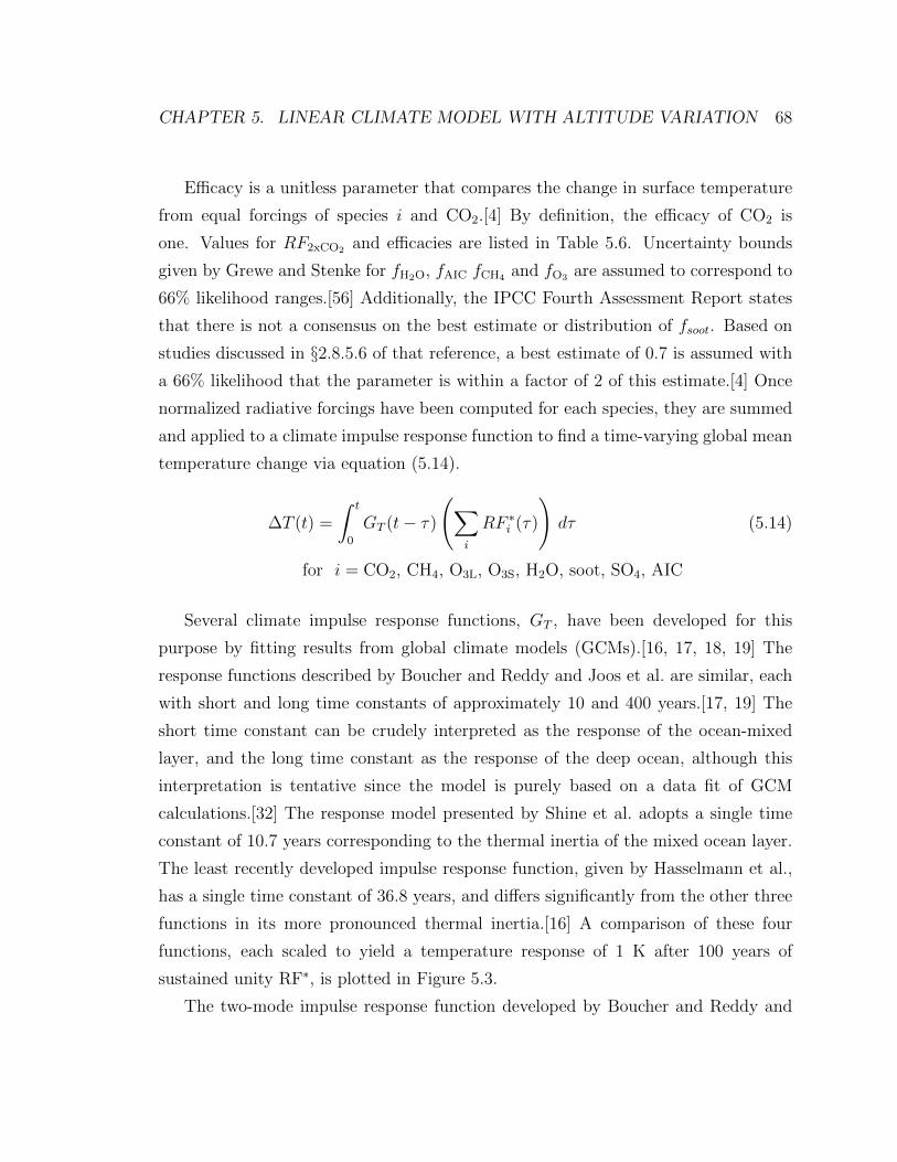
CHAPTER 5. LINEAR CLIMATE MODEL WITH ALTITUDE VARIATION 68
Efficacy is a unitless parameter that compares the change in surface temperature
from equal forcings of species i and CO2.[4] By definition, the efficacy of CO2 is
one. Values for RF2xCO2 and efficacies are listed in Table 5.6. Uncertainty bounds
given by Grewe and Stenke for fH2O, fAIC fCH4 and fO3 are assumed to correspond to
66% likelihood ranges.[56] Additionally, the IPCC Fourth Assessment Report states
that there is not a consensus on the best estimate or distribution of fsoot. Based on
studies discussed in §2.8.5.6 of that reference, a best estimate of 0.7 is assumed with
a 66% likelihood that the parameter is within a factor of 2 of this estimate.[4] Once
normalized radiative forcings have been computed for each species, they are summed
and applied to a climate impulse response function to find a time-varying global mean
temperature change via equation (5.14).
∆T (t) =
∫ t
0
GT (t− τ)
(∑i
RF ∗i (τ)
)dτ (5.14)
for i = CO2, CH4, O3L, O3S, H2O, soot, SO4, AIC
Several climate impulse response functions, GT , have been developed for this
purpose by fitting results from global climate models (GCMs).[16, 17, 18, 19] The
response functions described by Boucher and Reddy and Joos et al. are similar, each
with short and long time constants of approximately 10 and 400 years.[17, 19] The
short time constant can be crudely interpreted as the response of the ocean-mixed
layer, and the long time constant as the response of the deep ocean, although this
interpretation is tentative since the model is purely based on a data fit of GCM
calculations.[32] The response model presented by Shine et al. adopts a single time
constant of 10.7 years corresponding to the thermal inertia of the mixed ocean layer.
The least recently developed impulse response function, given by Hasselmann et al.,
has a single time constant of 36.8 years, and differs significantly from the other three
functions in its more pronounced thermal inertia.[16] A comparison of these four
functions, each scaled to yield a temperature response of 1 K after 100 years of
sustained unity RF∗, is plotted in Figure 5.3.
The two-mode impulse response function developed by Boucher and Reddy and

CHAPTER 5. LINEAR CLIMATE MODEL WITH ALTITUDE VARIATION 69
0 20 40 60 80 1000
0.02
0.04
0.06
0.08
0.1
0.12
0.14
0.16
time [yrs]
scal
ed te
mpe
ratu
re im
puls
e re
spon
se
functions scaled so that responseto unity step at t=100 is 1
shaded area is 66% likelihood range
Hasselmann (1993)Joos (2001)Shine (2005)Boucher (2008)
Figure 5.3: Scaled temperature impulse response functions from Hasselmann et al.,Joos et al., Shine et al., and Boucher and Reddy.[16, 17, 18, 19]
given in equation (5.15) is applied in this model.[19] The climate sensitivity parameter,
S, is the steady-state temperature change that would result from a constant annual
forcing of RF2xCO2 . Probability distributions of the parameters αt, τt1, and τt2 are
approximated based on the four impulse response functions plotted in Figure 5.3,
with emphasis on the more recent models of Joos et al., Shine et al., and Boucher
and Reddy. The estimated two-thirds likelihood range for GT (t) is shown in Figure
5.3, and parameter distributions are listed in Table 5.6.
GT (t) = S
[αtτt1
exp
(−tτt1
)+
1− αtτt2
exp
(−tτt2
)](5.15)
5.5 Limitations of the Climate Model
Linear climate models offer many advantages compared with more complex models,
including lower computational costs and increased transparency. The IPCC has noted

CHAPTER 5. LINEAR CLIMATE MODEL WITH ALTITUDE VARIATION 70
TemperatureBest Estimate Distribution 90% Likelihood Range
Model Parameter
fCH4 1.18 [68] normal 0.977, 1.38 [56]
fH2O 1.14 [68] normal 0.550, 1.73 [56]
fO3 1.37 [68] normal 0.662, 2.08 [56]
fSO4 0.9 [4]a normal 0.412, 1.39 [4]a
fsoot 0.7 [4]a lognormal 0.212, 2.31 [4]a
fAIC 0.59 [68] normal 0.488, 0.692 [56]
RF2xCO2 3.70 W/m2 [4]b normal 3.33, 4.07 [4]b
S 3.0 K [4]c lognormal 1.49, 6.03 [4]c
αt 0.595 [19] lognormal 0.397, 0.893 [see text]
τt1 8.4 yrs [19] lognormal 4.2, 16.8 [see text]
τt2 409.5 yrs [19] lognormal 205, 819 [see text]
a IPCC 2007, WG1, §2.8.5.5 and §2.8.5.6b IPCC 2007, WG1, §2.3.1c IPCC 2007, WG1, Box 10.2
Table 5.6: Temperature change model parameter values and distribu-tions.
these benefits and applies rapid, low cost climate response calculations based on pa-
rameterizations of global climate models.[4, 1] However, accompanying these benefits
are several limitations.
The temperature change computed in this model is based on a global mean re-
sponse to radiative forcings that can be produced either globally or regionally. CO2
has a long lifetime, allowing the gas to mix throughout the atmosphere so that ra-
diative forcing is independent from emission location. Shorter-lived perturbations,
such as ozone production from NOx emissions, cause radiative forcing only near flight
routes. Thus, radiative forcings due to O3 production and aviation induced cloudi-
ness are greatest in the northern mid-latitudes where aircraft traffic is most dense.[3]
As a result, a scenario of net zero forcing may induce strong regional positive and
negative temperature responses.[22] This study does not consider varying regional

CHAPTER 5. LINEAR CLIMATE MODEL WITH ALTITUDE VARIATION 71
impacts from aircraft emissions and instead focuses on the climate response averaged
over the Earth’s surface.
As noted above, models for radiative forcing from all emissions except CO2, which
has a very long atmospheric lifetime, are dependent on the assumed temporal and
geographical distribution of emissions. The RF computed in this model is not the
forcing of one single aircraft, on a single mission, at a single time and location;
rather it is the forcing caused by a fleet of many aircraft of a single type, operated
continuously and globally. The models used here are based on average impacts from
fleetwide routing in a single year within the last decade. This routing is concentrated
largely in the northern hemisphere mid-latitudes. These models therefore quantify the
average forcing caused by emissions spatially and temporally distributed according
to routing similar to current traffic. Assumptions about flight timing are particularly
important for contrail impacts, which can vary both seasonally and diurnally.[35] If
the route distribution for a particular aircraft fleet differs significantly from current
routing, then estimates of model parameter values become less accurate.
This linear climate model does not capture many of the sensitivities that are
included in comprehensive assessments by global climate models. For instance, emis-
sions from non-aviation sources may alter climate parameters.[1] Also, the effects
of some aviation emissions are chemically coupled but are assumed to be indepen-
dent in this model, such as NOx and SOx, which are interdependent through OH
chemistry.[22] And as noted by Wuebbles et al., the quality of a simple parameter-
ization is limited by the accuracy of the global model upon which it is based.[51]
This model adopts the most recent, established methods of this type for computing
radiative forcing and temperature change. However, as climate knowledge is refined
in the future, this model can be updated to incorporate best available information.
CO2 radiative forcing is calculated with the carbon cycle model of Boucher and
Reddy which was applied by the IPCC for computing global warming potentials.
This model assumes constant background CO2 concentrations of 378 ppmv, a likely
underestimate of actual near-term concentrations. As a result, the impacts of CO2
emissions are overvalued by an amount that varies depending on the chosen metric.

CHAPTER 5. LINEAR CLIMATE MODEL WITH ALTITUDE VARIATION 72
The impact of background CO2 concentration scenario assumptions is addressed in
uncertainty discussions in Chapter 6.
NOx and AIC models average and greatly simplify the effects of the complex pro-
cesses associated with forcing from ozone production and cloud formation, leading to
large uncertainty. Models of ozone formation are complicated by nonlinear produc-
tion rates that are sensitive to background composition and meteorological conditions.
Moreover, the temperature response to equal ozone production forcings can vary with
latitude and altitude due to strong dependence on local feedbacks.[52, 22] The short-
lived ozone model presented here only attempts to capture the effects of varying
altitude. However, on a globally-averaged scale, several studies have demonstrated a
linear relationship between ozone production forcing and aircraft NOx emissions.[1]
Furthermore, the AIC forcing model scales simply with flight distance and does
not reflect variation in impact with changing particle and water vapor emissions or
exhaust temperature. The assumption that AIC forcing is proportional to flight
distance may lead to an upper bound estimate of AIC impacts because it is likely
that cloud cover will saturate in high density air traffic regions.[1] The forcing models
applied here are based on results from global climate models; however, the level of
scientific understanding of AIC impact estimation is still poor, particularly for induced
cirrus cloudiness. It is expected that AIC models will be refined in the future as the
climate modeling community achieves a better understanding of AIC impacts.
5.6 Uncertainty Quantification
Because of their low computational costs, linear climate models enable users to ex-
plore the climate responses of many scenarios and sensitivities to uncertain model
parameters.[4] This section describes methods for quantifying the overall uncertainty
in temperature change estimates produced with this climate model.
A number of sources of uncertainty exist in estimating the relative climate im-
pacts of different aircraft.[67] Scientific uncertainty is the focus of this study and is
associated with limits in scientific knowledge and inexact modeling approaches for
quantifying impacts from an emissions scenario. Other sources include valuation and

CHAPTER 5. LINEAR CLIMATE MODEL WITH ALTITUDE VARIATION 73
scenario uncertainty. The selection of a climate metric, with explicit or implicit tem-
poral weighting of impacts, affects the relative importance of short-term and long-term
impacts and therefore involves valuation uncertainty. The climate metric adopted for
studies in this research, ATR, is described in Chapter 3. Valuation uncertainty is
not addressed directly, and these judgments are instead presented as user-specified
inputs in the ATR framework. Scenario uncertainty refers to unknowns surround-
ing the projections of future anthropogenic activities and system responses that are
required to estimate aircraft climate impacts. Scenario assumptions are implicit in
the linear climate model presented in this chapter. The linear CO2 radiative forcing
model assumes constant background concentrations. The impact of this assumption
is investigated by comparing results to a model with varying background concentra-
tions. The climate model also assumes that physical climate responses will not change
in the future, or in other words, that climate feedback mechanisms and all species’
radiative efficiencies remain constant. This uncertainty is not quantified in this study
and relates to future scenarios that are difficult to predict.
Scientific uncertainty is assessed by analyzing the uncertainty in each component
of the climate model to construct information about the uncertainty of model out-
puts. Exact values of parameters used in the linear climate model are not known;
instead, parameters can be more appropriately described by probability distributions
over a range of possible parameter values. Distribution information for each model
parameter is listed in Table 5.3, 5.4, 5.5, or 5.6. It should be noted that climate
sensitivity, S, is a scaling value applied to all temperature calculations. This research
is concerned with the relative impacts of competing aircraft designs, and this pa-
rameter’s uncertainty is excluded because it has no effect on relative climate impact.
Following Lee et al., the uncertainties in NOx-induced radiative forcing parameters
(ACH4 , AO3L, and
(RFref
Eref
)O3S
) are likely to be coupled. Correlation coefficients of 0.5
are assumed between these three parameters.[1] All other uncertain parameters are
assumed to be independent.
Uncertainties in forcing factor functions are based on uncertainty in data forRFiENOx
(h) and RFAIC
L(h).[14, 15] This information is used to calculate si(h) via equations
(5.5) and (5.6). Probability distributions forRFCH4
ENOx(h) and
RFO3S
ENOx(h) are assumed to
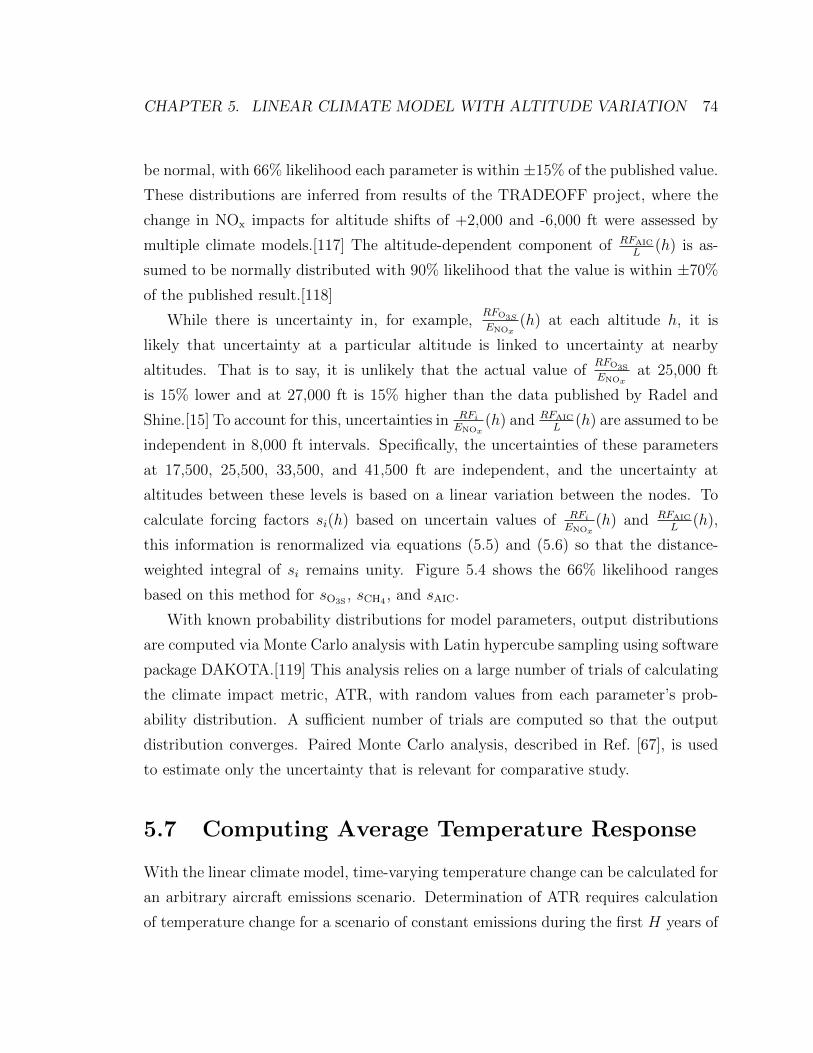
CHAPTER 5. LINEAR CLIMATE MODEL WITH ALTITUDE VARIATION 74
be normal, with 66% likelihood each parameter is within ±15% of the published value.
These distributions are inferred from results of the TRADEOFF project, where the
change in NOx impacts for altitude shifts of +2,000 and -6,000 ft were assessed by
multiple climate models.[117] The altitude-dependent component of RFAIC
L(h) is as-
sumed to be normally distributed with 90% likelihood that the value is within ±70%
of the published result.[118]
While there is uncertainty in, for example,RFO3S
ENOx(h) at each altitude h, it is
likely that uncertainty at a particular altitude is linked to uncertainty at nearby
altitudes. That is to say, it is unlikely that the actual value ofRFO3S
ENOxat 25,000 ft
is 15% lower and at 27,000 ft is 15% higher than the data published by Radel and
Shine.[15] To account for this, uncertainties in RFiENOx
(h) and RFAIC
L(h) are assumed to be
independent in 8,000 ft intervals. Specifically, the uncertainties of these parameters
at 17,500, 25,500, 33,500, and 41,500 ft are independent, and the uncertainty at
altitudes between these levels is based on a linear variation between the nodes. To
calculate forcing factors si(h) based on uncertain values of RFiENOx
(h) and RFAIC
L(h),
this information is renormalized via equations (5.5) and (5.6) so that the distance-
weighted integral of si remains unity. Figure 5.4 shows the 66% likelihood ranges
based on this method for sO3S, sCH4 , and sAIC.
With known probability distributions for model parameters, output distributions
are computed via Monte Carlo analysis with Latin hypercube sampling using software
package DAKOTA.[119] This analysis relies on a large number of trials of calculating
the climate impact metric, ATR, with random values from each parameter’s prob-
ability distribution. A sufficient number of trials are computed so that the output
distribution converges. Paired Monte Carlo analysis, described in Ref. [67], is used
to estimate only the uncertainty that is relevant for comparative study.
5.7 Computing Average Temperature Response
With the linear climate model, time-varying temperature change can be calculated for
an arbitrary aircraft emissions scenario. Determination of ATR requires calculation
of temperature change for a scenario of constant emissions during the first H years of

CHAPTER 5. LINEAR CLIMATE MODEL WITH ALTITUDE VARIATION 75
Figure 5.4: Forcing factors (lines) with 66% likelihood ranges (shaded areas). Alti-tudes with forcing factors based on raditiave forcing data with independent probabil-ity distributions are marked with black points.
operation and zero emissions thereafter. This yields the quantity ∆Tsust,H(t), defined
in equation (5.16).
∆Tsust,H(t) = ∆T (t)∣∣∣si=si, Ei(t)=ei Usust σH(t)
(5.16)
σH(t) =
1 t ≤ H
0 H < t ≤ tmax
In equation (5.16), the index i includes all radiatively active emissions and effects
(CO2, NOx, H2O, SO4, soot, and AIC). Emissions rates are based on the performance
of a particular aircraft on a specified mission. Sustained utilization rate, Usust, is con-
stant between configurations and years, and its value does not matter for comparative
studies. The function σH(t) is a unity backward step, which characterizes the input
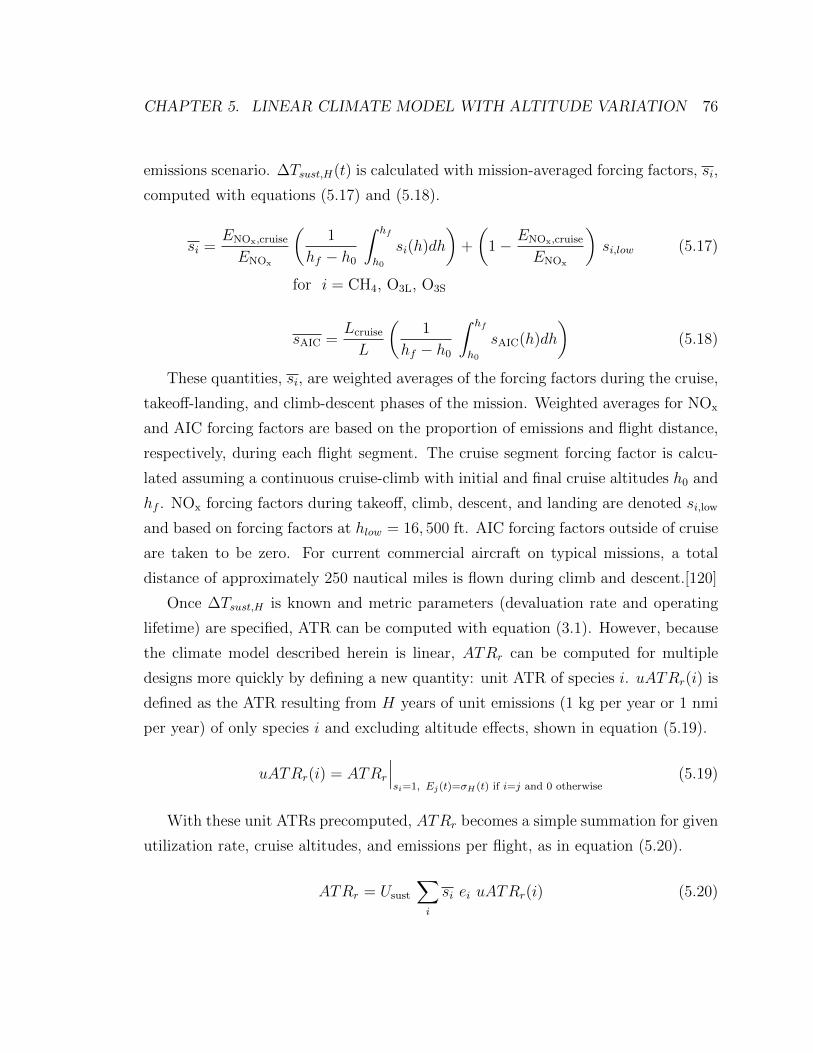
CHAPTER 5. LINEAR CLIMATE MODEL WITH ALTITUDE VARIATION 76
emissions scenario. ∆Tsust,H(t) is calculated with mission-averaged forcing factors, si,
computed with equations (5.17) and (5.18).
si =ENOx,cruise
ENOx
(1
hf − h0
∫ hf
h0
si(h)dh
)+
(1− ENOx,cruise
ENOx
)si,low (5.17)
for i = CH4, O3L, O3S
sAIC =Lcruise
L
(1
hf − h0
∫ hf
h0
sAIC(h)dh
)(5.18)
These quantities, si, are weighted averages of the forcing factors during the cruise,
takeoff-landing, and climb-descent phases of the mission. Weighted averages for NOx
and AIC forcing factors are based on the proportion of emissions and flight distance,
respectively, during each flight segment. The cruise segment forcing factor is calcu-
lated assuming a continuous cruise-climb with initial and final cruise altitudes h0 and
hf . NOx forcing factors during takeoff, climb, descent, and landing are denoted si,low
and based on forcing factors at hlow = 16, 500 ft. AIC forcing factors outside of cruise
are taken to be zero. For current commercial aircraft on typical missions, a total
distance of approximately 250 nautical miles is flown during climb and descent.[120]
Once ∆Tsust,H is known and metric parameters (devaluation rate and operating
lifetime) are specified, ATR can be computed with equation (3.1). However, because
the climate model described herein is linear, ATRr can be computed for multiple
designs more quickly by defining a new quantity: unit ATR of species i. uATRr(i) is
defined as the ATR resulting from H years of unit emissions (1 kg per year or 1 nmi
per year) of only species i and excluding altitude effects, shown in equation (5.19).
uATRr(i) = ATRr
∣∣∣si=1, Ej(t)=σH(t) if i=j and 0 otherwise
(5.19)
With these unit ATRs precomputed, ATRr becomes a simple summation for given
utilization rate, cruise altitudes, and emissions per flight, as in equation (5.20).
ATRr = Usust
∑i
si ei uATRr(i) (5.20)

CHAPTER 5. LINEAR CLIMATE MODEL WITH ALTITUDE VARIATION 77
Species, i uATRr=0(i) uATRr=1%(i) uATRr=3%(i) uATRr=∞(i)
CO2 1.66 x10⁻¹³ 4.36x10⁻¹⁴ 1.96x10⁻¹⁴ 5.59x10⁻¹⁵ K per kg CO2
CH4 -4.76x10⁻¹² -3.40x10⁻¹² -2.78x10⁻¹² -1.44x10⁻¹² K per kg NOx
O3S 9.46x10⁻¹² 7.19x10⁻¹² 6.46x10⁻¹² 4.85x10⁻¹² K per kg NOx
O3L -1.29x10⁻¹² -9.25x10⁻¹³ -7.57x10⁻¹³ -3.91x10⁻¹³ K per kg NOx
H2O 5.77x10⁻¹⁵ 4.38x10⁻¹⁵ 3.94x10⁻¹⁵ 2.96x10⁻¹⁵ K per kg H2O
SO4 -6.13x10⁻¹¹ -4.66x10⁻¹¹ -4.18x10⁻¹¹ -3.14x10⁻¹¹ K per kg SO4
soot 2.38x10⁻¹⁰ 1.81x10⁻¹⁰ 1.63x10⁻¹⁰ 1.22x10⁻¹⁰ K per kg soot
AIC 8.90x10⁻¹³ 6.76x10⁻¹³ 6.07x10⁻¹³ 4.56x10⁻¹³ K per nmi
Table 5.7: Values of unit ATRs for H = 30 years, tmax = 500 years, and four differentvalues of r calculated with a linear climate model.
Unit ATRs are calculated for several devaluation rates, an operating lifetime of 30
years, and a maximum integration period of 500 years in Table 5.7. These parameters
are computed using the climate model described in this chapter. As more knowledge
is gained, this climate model can be refined, and updated values for uATR should be
applied.

Chapter 6
Aircraft Design Studies
6.1 Introduction
Commercial aviation emissions have grown over the past several decades despite im-
provements in fuel efficiency. A portion of these emissions affect the radiative balance
of the Earth system, causing radiative forcing and climate change. The fraction of an-
thropogenic radiative forcing attributed to aviation is projected to rise,[1] and changes
in aircraft operations and design may be necessary to meet goals for limiting climate
change. This chapter investigates methods for reducing the climate impacts of future
aircraft and quantifies the effects of these mitigation strategies on aircraft perfor-
mance and operating costs. Several methods are explored, although policy options
are not considered. First, because the magnitude of impacts from NOx emissions and
AIC effects vary with altitude, one mitigation strategy involves designing aircraft to
fly at altitudes with lower climate impact sensitivities. Past studies have investigated
the climate impacts of shifting fleet altitudes, each generally demonstrating potential
climate savings for flight at lower altitudes (e.g., Refs. [121, 117, 122, 123, 15, 14]).
Secondly, the effects of technologies aimed at reducing aircraft climate impacts are
assessed. This research focuses on near-term technologies and conventional aircraft
configurations, although significant climate impact savings may be possible with non-
hydrocarbon energy sources and less conventional aircraft such as blended wing bod-
ies. Some of the technologies investigated, including drop-in alternative fuels and
78

CHAPTER 6. AIRCRAFT DESIGN STUDIES 79
operational contrail avoidance, can also be applied to the existing fleet in addition
to future aircraft. In this chapter, narrowbody aircraft are assessed and the same
conclusions are expected to apply to larger aircraft.[124]
6.2 Aircraft Optimization Problem
Aircraft analysis is performed using the conceptual design tool PASS (Program for
Aircraft Synthesis Studies), described in Chapter 4. This tool integrates a set of
industry design methods to compute aircraft performance based on aircraft design
variables.[74] Aircraft climate impacts are computed with the climate model dis-
cussed in Chapter 5 and measured using the average temperature response (ATR)
metric defined in Chapter 3 with two devaluation rates: 0% and 3%. These tools are
combined with an optimizer to find the aircraft design parameter values that minimize
a specified performance objective such as cost or average temperature response.
The set of aircraft studied carry 162 passengers and have payload, range, and
performance requirements similar to those of a 737-800. Technology levels assumed for
these aircraft are consistent with an entry-into-service year of 2010. Cost calculations
are based on constant 2010 labor rates and a constant jet-A fuel price of $2.25 per
gallon, unless otherwise noted. The distances flown during most commercial airline
missions are considerably shorter in length than the aircraft’s maximum design range
(3,000 nautical miles). For this reason, aircraft are optimized for performance on
a “typical mission” while at the same time constrained to meet maximum design
range requirements. A typical mission is defined as a flight with the design payload
and a stage length of 1,000 nautical miles, based on the average narrowbody stage
length for US carriers.[125] Each aircraft is designed with identical fuselage geometry
but varying wing, engine, and mission design parameters. All configurations must
meet the same takeoff, climb, cruise, and landing requirements. Optimization design
variables and imposed constraints are listed in Tables 6.1 and 6.2.
Aircraft are designed to minimize a combination of operating costs, emissions,
and ATR. A gradient-based method is used to solve this constrained optimization
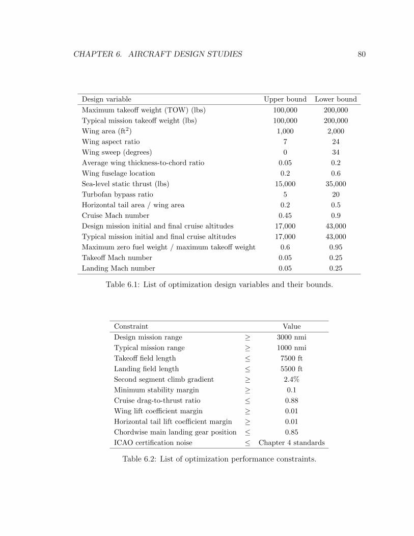
CHAPTER 6. AIRCRAFT DESIGN STUDIES 80
Design variable Upper bound Lower bound
Maximum takeoff weight (TOW) (lbs) 100,000 200,000
Typical mission takeoff weight (lbs) 100,000 200,000
Wing area (ft2) 1,000 2,000
Wing aspect ratio 7 24
Wing sweep (degrees) 0 34
Average wing thickness-to-chord ratio 0.05 0.2
Wing fuselage location 0.2 0.6
Sea-level static thrust (lbs) 15,000 35,000
Turbofan bypass ratio 5 20
Horizontal tail area / wing area 0.2 0.5
Cruise Mach number 0.45 0.9
Design mission initial and final cruise altitudes 17,000 43,000
Typical mission initial and final cruise altitudes 17,000 43,000
Maximum zero fuel weight / maximum takeoff weight 0.6 0.95
Takeoff Mach number 0.05 0.25
Landing Mach number 0.05 0.25
Table 6.1: List of optimization design variables and their bounds.
Constraint Value
Design mission range ≥ 3000 nmi
Typical mission range ≥ 1000 nmi
Takeoff field length ≤ 7500 ft
Landing field length ≤ 5500 ft
Second segment climb gradient ≥ 2.4%
Minimum stability margin ≥ 0.1
Cruise drag-to-thrust ratio ≤ 0.88
Wing lift coefficient margin ≥ 0.01
Horizontal tail lift coefficient margin ≥ 0.01
Chordwise main landing gear position ≤ 0.85
ICAO certification noise ≤ Chapter 4 standards
Table 6.2: List of optimization performance constraints.

CHAPTER 6. AIRCRAFT DESIGN STUDIES 81
problem. Economic and environmental performance is compared for a variety of
technology scenarios in the following sections.
6.3 Results with Baseline Technology
First, optimization results are presented for designs using conventional technologies
likely to be applied on an airliner entering service in 2010. These baseline technologies
include a lightweight composite structure and advanced, high bypass ratio turbofan
engines. Combustor performance is comparable to recently certified engines with a
NOx emissions index model based on the GE90-85B dual annular combustor, see
Chapter 5. In this section, instead of applying technologies aimed at reduced climate
impacts, the effects of varied wing and engine design variables, cruise speed, and
altitudes are considered. First, single-objective optimization results for minimum
cost, emissions, and climate impact aircraft are discussed. Then, multi-objective
results are presented, featuring designs with concurrently optimal cost and climate
performance.
6.3.1 Single-Objective Results
Aviation induced cloudiness and emissions of CO2 and NOx combine to produce the
majority of commercial aviation’s climate impacts. One method to reduce the net
climate impacts of future aircraft is to design for reduced emissions. Table 6.3 com-
pares aircraft designed to minimize five different objective functions: total operating
costs, total fuel burn (directly proportional to CO2 emissions), total NOx emissions,
ATRr=0, and ATRr=3.
The minimum cost aircraft represents the most economically competitive design
that also meets current safety and environmental regulations. This configuration is
generally similar to current aircraft operating in the single aisle, medium range mar-
ket, but has improved performance, reflecting 2010 technology levels. The aircraft
cruises near Mach 0.84 and features a moderate aspect ratio, highly swept wing and
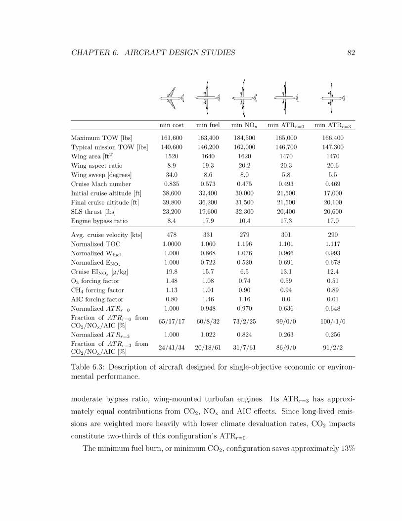
CHAPTER 6. AIRCRAFT DESIGN STUDIES 82
min cost min fuel min NOx min ATRr=0 min ATRr=3
Maximum TOW [lbs] 161,600 163,400 184,500 165,000 166,400
Typical mission TOW [lbs] 140,600 146,200 162,000 146,700 147,300
Wing area [ft2] 1520 1640 1620 1470 1470
Wing aspect ratio 8.9 19.3 20.2 20.3 20.6
Wing sweep [degrees] 34.0 8.6 8.0 5.8 5.5
Cruise Mach number 0.835 0.573 0.475 0.493 0.469
Initial cruise altitude [ft] 38,600 32,400 30,000 21,500 17,000
Final cruise altitude [ft] 39,800 36,200 31,500 21,500 20,100
SLS thrust [lbs] 23,200 19,600 32,300 20,400 20,600
Engine bypass ratio 8.4 17.9 10.4 17.3 17.0
Avg. cruise velocity [kts] 478 331 279 301 290
Normalized TOC 1.0000 1.060 1.196 1.101 1.117
Normalized Wfuel 1.000 0.868 1.076 0.966 0.993
Normalized ENOx1.000 0.722 0.520 0.691 0.678
Cruise EINOx[g/kg] 19.8 15.7 6.5 13.1 12.4
O3 forcing factor 1.48 1.08 0.74 0.59 0.51
CH4 forcing factor 1.13 1.01 0.90 0.94 0.89
AIC forcing factor 0.80 1.46 1.16 0.0 0.01
Normalized ATRr=0 1.000 0.948 0.970 0.636 0.648
Fraction of ATRr=0 fromCO2/NOx/AIC [%]
65/17/17 60/8/32 73/2/25 99/0/0 100/-1/0
Normalized ATRr=3 1.000 1.022 0.824 0.263 0.256
Fraction of ATRr=3 fromCO2/NOx/AIC [%]
24/41/34 20/18/61 31/7/61 86/9/0 91/2/2
Table 6.3: Description of aircraft designed for single-objective economic or environ-mental performance.
moderate bypass ratio, wing-mounted turbofan engines. Its ATRr=3 has approxi-
mately equal contributions from CO2, NOx and AIC effects. Since long-lived emis-
sions are weighted more heavily with lower climate devaluation rates, CO2 impacts
constitute two-thirds of this configuration’s ATRr=0.
The minimum fuel burn, or minimum CO2, configuration saves approximately 13%

CHAPTER 6. AIRCRAFT DESIGN STUDIES 83
in fuel consumption relative to the minimum cost design. Since the aircraft cruises
at a much slower Mach 0.57, the wings are designed with a high aspect ratio and low
sweep, leading to lower induced drag. Reduced drag allows the aircraft to meet climb
requirements with smaller engines. This configuration also uses higher bypass ratio
turbofan engines with decreased thrust specific fuel consumption. Despite savings in
fuel costs, this low speed design has 6% higher total operating costs, owing to lower
per-unit utilization rates and increased crew and maintenance costs associated with
long flight times. The minimum fuel aircraft flies approximately 5,000 ft lower than
the minimum cost aircraft in a region where contrail formation is more likely; even
though fuel burn is 13% lower, only 5.2% savings in ATRr=0 and a 2.2% penalty in
ATRr=3 are realized compared with the reference aircraft.
The minimum NOx aircraft emits nearly 50% less NOx compared with the min-
imum cost design. This configuration has very high thrust engines so that during
cruise the engines can be throttled back, yielding an extremely low emissions index.
However, the resulting heavy airframe and low flight speed cause this design’s oper-
ating costs to escalate relative to the other four configurations. As with the low fuel
aircraft, the low NOx aircraft cruises at lower altitudes where contrail impacts are
more severe. A greater AIC forcing factor and higher fuel burn cancels out the benefit
of lower NOx emissions, as measured by ATRr=0. On the other hand, ATRr=3, which
is more sensitive to short-lived effects from NOx emissions, is reduced by 18%.
Lastly, two aircraft are designed to minimize climate impacts as measured by
ATR. These designs differ from the minimum emissions designs in their very low
design cruise altitudes. By cruising at Mach 0.5 and 20,000 ft, atmospheric impacts
from NOx, contrails, and cirrus are essentially eliminated and climate impacts are
almost entirely due to CO2 emissions. The minimum ATRr=3 configuration cruises at
slightly lower altitudes to reduce short-lived impacts at the expense of 3% higher fuel
burn and CO2 emissions. At this altitude, the cooling impacts from methane and long-
term ozone destruction exceed warming impacts from short-term ozone production,
and the net ATRr=0 due to NOx is negative. The resulting designs exhibit 35% lower
ATRr=0 and 74% lower ATRr=3 than the reference minimum cost aircraft. Operating
costs are penalized approximately 10-12%, primarily due to longer mission times.
CHAPTER 6. AIRCRAFT DESIGN STUDIES 84
These results draw attention to the difference in design characteristics and perfor-
mance between aircraft optimized for different environmental metrics. The minimum
NOx design has higher fuel burn than even the minimum cost design, even though
total emissions quantity depends directly on fuel consumption, see equation 5.2. The
minimum fuel burn design has little or no climate savings, measured by ATRr=0 and
ATRr=3 (5.2% or -2.2% compared with minimum cost value), despite large fuel sav-
ings (13%). Thus, designing an aircraft to be green by one environmental standard
does not ensure that the aircraft will be green in other environmental metrics, even
if all metrics are related to emissions and atmospheric impacts. In particular, design
cruise altitude has a powerful effect on the net climate impacts of a configuration.
6.3.2 Cost-Climate Tradeoff
For a low climate impact aircraft to be viable in the airline industry, it must also
perform competitively economically. This section assesses the relationship between
operating costs and climate impacts with conventional 2010 aircraft technology. By
optimizing designs for minimum ATR and varying constraints on cost, or vice versa,
a pareto front is generated. Figure 6.1 shows this tradeoff between cost and both
ATRr=0 and ATRr=3 for narrowbody configurations. Each point on the figure repre-
sents a separate design, optimized to minimize a different balance of economic and
climate performance. Details for the three extrema on the pareto fronts are provided
in Table 6.3. Reducing design cruise altitude and Mach number has a dramatic effect
on climate impacts measured by ATR, regardless of the devaluation rate. As the
figure shows, climate impact savings on the order of 35-75% are possible by flying
slower and lower than the present-day fleet. These low climate impact designs have
higher operating costs due largely to longer mission times. By reducing altitude by
about 12,000 ft to levels where both NOx and cloud impacts are less severe, ATRr=0
and ATRr=3 decrease by about 10% and 30%, respectively, for a 1% increase in total
operating costs.

CHAPTER 6. AIRCRAFT DESIGN STUDIES 85
0.98 1 1.02 1.04 1.06 1.08 1.1 1.120.1
0.2
0.3
0.4
0.5
0.6
0.7
0.8
0.9
1
1.1
0.8439/40
0.7739/400.7825/33
0.7725/31
0.7424/30
0.7122/28
0.6721/26
0.6121/23 0.54
21/220.4921/22
normalized total operating costs
norm
aliz
ed A
TR
objective: ATR
r=0
cruise Machinitial/final altitudes (kft)
ATRr=0
ATRr=3
(a) Optimized ATRr=0; evaluated ATRr=3 also shown.
0.98 1 1.02 1.04 1.06 1.08 1.1 1.120.1
0.2
0.3
0.4
0.5
0.6
0.7
0.8
0.9
1
1.1
0.8439/40
0.7839/40
0.7925/33
0.7825/31
0.7724/29
0.7521/27
0.7221/23
0.6519/22 0.54
17/210.4717/20
normalized total operating costs
norm
aliz
ed A
TR
objective: ATR
r=3
cruise Machinitial/final altitudes (kft)
ATRr=0
ATRr=3
(b) Optimized ATRr=3; evaluated ATRr=0 also shown.
Figure 6.1: Baseline designs optimized for minimum total operating costs and ATRwith two devaluation rates, r = 0 and r = 3%. Black points indicate designs withlisted cruise altitudes and Mach numbers.
Figure 6.1 includes results for two climate objective functions. Designs with opti-
mal ATRr=0 are discussed first, and later compared with optimal ATRr=3 configura-
tions. The lowest cost section of the pareto front in Figure 6.1(a) has a kink around
which the slope of the curve changes sharply. Beginning at the minimum cost point,
designs fly successively slower to improve aerodynamic efficiency and reduce thrust
required for climb. After reducing fuel burn by up to approximately 5% by cruis-
ing slower, climate impacts can be reduced more drastically by flying at much lower
altitudes. The point that separates these high and low altitude designs is indicated
on Figure 6.1(a) by the second lowest cost black point. This design cruises between
39,000 and 40,000 ft at Mach 0.77 and has smaller engines and a lighter airframe than
lower cost designs. Pareto optimal designs with lower ATRr=0 cruise at altitudes of at
most 34,000 ft. At lower altitudes, reductions in NOx and AIC forcing factors more
than offset the increase in fuel burn from flying in denser air. Additionally, more
thrust is available at lower altitudes, allowing the engines to be throttled back, which
reduces internal combustor temperatures, and consequently, cruise NOx emissions in-
dices. From this kink point, further reductions in climate impacts are achieved by

CHAPTER 6. AIRCRAFT DESIGN STUDIES 86
flying at even lower altitudes and speeds. ATRr=0 is minimized at a cruise altitude
near 22,000 ft.
Figure 6.1(b) indicates similar findings for designs optimized with the climate
objective function ATRr=3. This metric devaluation applies a lower weighting to long-
lived CO2 impacts. Thus, the pareto front more quickly shifts to low altitude, higher
fuel burn designs, resulting in configurations with lower ATRr=3 but higher ATRr=0.
Optimal ATRr=3 designs cruise at slightly faster speeds than optimal ATRr=0 designs,
trading lower mission times for greater fuel burn. Results with these two objective
functions are otherwise similar; because of this, for the remainder of this chapter,
only results for the climate objective function ATRr=0 are presented.
6.4 Results with Climate Mitigation Technologies
Design optimization results for the baseline technology scenario illustrate the strong
dependence of climate impacts, as measured by ATR, on design cruise altitude and
speed. Through application of climate impact reduction technologies, significant de-
creases in climate impacts may be possible with smaller penalties to total operating
costs. A number of previous studies have reviewed climate mitigation technologies
and operational strategies (e.g., Refs. [24, 25, 26, 22]). This section explores the po-
tential benefits of several green technologies: propfan engines, natural laminar flow,
alternative fuels, low NOx combustors, and contrail avoidance. The list of mitigation
strategies investigated is not intended to be comprehensive, but instead explores the
benefits of a few key technologies that could be applied to aircraft in the next 10-20
years. The effects of climate change policy options are not assessed in this research.
6.4.1 CO2 Impact Reduction
CO2 emissions affect global climate on timescales much longer than other aircraft
emissions, causing residual temperature change for many hundreds of years after
release into the atmosphere. CO2 emissions are directly proportional to fuel con-
sumption, leading to two methods to mitigate impacts: reducing fuel burn or using a

CHAPTER 6. AIRCRAFT DESIGN STUDIES 87
fuel with lower CO2 intensity. The potential for fuel savings by designing aircraft for
slower cruise speeds is discussed in the previous section. Technologies such as open
rotor engines and laminar flow also provide fuel savings, particularly when applied
to aircraft with reduced cruise speeds relative to present-day commercial transports.
In addition to low fuel burn technologies, the substitution of biofuels for traditional
petroleum-based fuels could reduce or even eliminate the climate impacts of aviation
CO2 emissions.
Propfan Engines
Propfan engines, also known as open rotors, are unducted, very high bypass ratio
engines. Unlike traditional turboprop engines, propfans feature highly swept blades,
allowing for efficient performance at speeds of up to Mach 0.8.[82] These engines
achieve high propulsive efficiency without the weight and drag penalties associated
with large fan nacelles of comparable bypass ratio turbofans. Both single and dual
rotor propfans could be considered for application on future commercial aircraft, with
counter-rotating propfans being more efficient but noisier. Performance, weight, and
drag models for propfan engines are described in detail in Chapter 4. Following
Goldsmith, a fuselage weight penalty of 500 pounds is applied to propfan configu-
rations for cabin interior noise insulation.[126] To account for the fewer number of
seats with engine noise exposure on configuration with aft fuselage mounted engines,
this weight penalty is reduced by 25%. Figure 6.2 compares the economic and cli-
mate performance of configurations with turbofan and dual and single rotor propfan
engines. Because of the high uncertainty in estimating weight and performance of
future propfan engines, the effects of a 5% increase in specific fuel consumption and
a 20% increase in weight on dual rotor propfans are also shown in Figure 6.2.
A number of technical challenges exist in the development of propfan engines,
including community noise concerns. The lack of fan casing makes acoustic treat-
ment more difficult. A recent workshop of academia and industry concluded that
advanced open rotors are likely to “comfortably” meet current Chapter 4 noise cer-
tification standards, particularly if operational procedures are designed to minimize
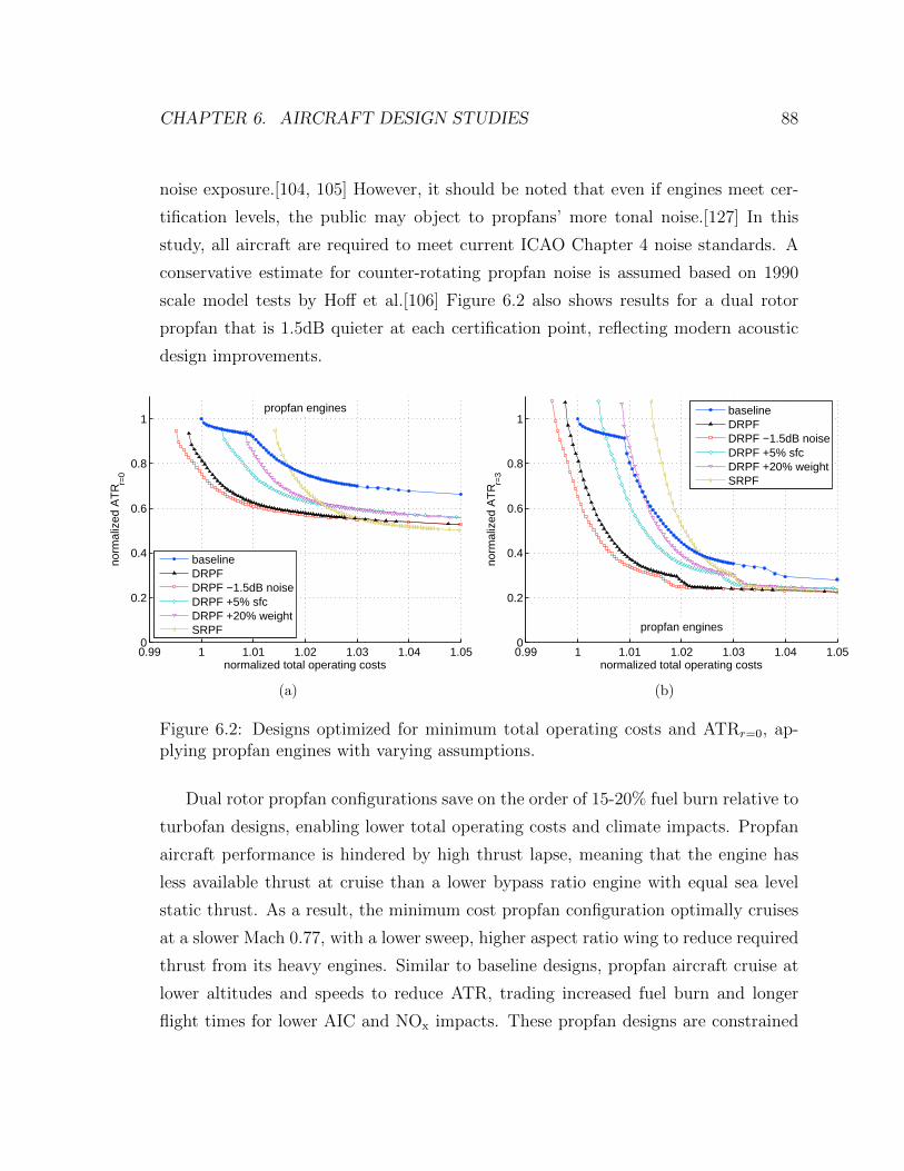
CHAPTER 6. AIRCRAFT DESIGN STUDIES 88
noise exposure.[104, 105] However, it should be noted that even if engines meet cer-
tification levels, the public may object to propfans’ more tonal noise.[127] In this
study, all aircraft are required to meet current ICAO Chapter 4 noise standards. A
conservative estimate for counter-rotating propfan noise is assumed based on 1990
scale model tests by Hoff et al.[106] Figure 6.2 also shows results for a dual rotor
propfan that is 1.5dB quieter at each certification point, reflecting modern acoustic
design improvements.
0.99 1 1.01 1.02 1.03 1.04 1.050
0.2
0.4
0.6
0.8
1
normalized total operating costs
norm
aliz
ed A
TR
r=0
propfan engines
baselineDRPFDRPF −1.5dB noiseDRPF +5% sfcDRPF +20% weightSRPF
(a)
0.99 1 1.01 1.02 1.03 1.04 1.050
0.2
0.4
0.6
0.8
1
normalized total operating costs
norm
aliz
ed A
TR
r=3
propfan engines
baselineDRPFDRPF −1.5dB noiseDRPF +5% sfcDRPF +20% weightSRPF
(b)
Figure 6.2: Designs optimized for minimum total operating costs and ATRr=0, ap-plying propfan engines with varying assumptions.
Dual rotor propfan configurations save on the order of 15-20% fuel burn relative to
turbofan designs, enabling lower total operating costs and climate impacts. Propfan
aircraft performance is hindered by high thrust lapse, meaning that the engine has
less available thrust at cruise than a lower bypass ratio engine with equal sea level
static thrust. As a result, the minimum cost propfan configuration optimally cruises
at a slower Mach 0.77, with a lower sweep, higher aspect ratio wing to reduce required
thrust from its heavy engines. Similar to baseline designs, propfan aircraft cruise at
lower altitudes and speeds to reduce ATR, trading increased fuel burn and longer
flight times for lower AIC and NOx impacts. These propfan designs are constrained

CHAPTER 6. AIRCRAFT DESIGN STUDIES 89
by Chapter 4 noise limits, causing designs to takeoff over a shorter distance to reduce
takeoff noise and have a larger wing and lower thrust engines than would be otherwise
optimal. The cost of this design constraint is illustrated by comparing results with
quieter dual rotor propfans, which meet noise constraints with a margin. Also shown
are results for dual rotor propfan configurations with less efficient and heavier engines,
which burn 2-5% more fuel burn than reference propfan designs. These fuel burn
penalties eliminate the operating cost savings of propfan engines. Finally, single
rotor propfan configurations are penalized in the simple swirl loss model applied
here, causing optimized configurations to cruise at slower speeds. As a result, single
rotor propfan configurations have higher operating costs than baseline designs despite
having very low specific fuel consumption.
Natural Laminar Flow
Aircraft fuel consumption can be improved through reductions in profile drag, with
skin friction accounting for about half of conventional aircraft drag at cruise.[26] By
designing surfaces to maintain laminar boundary layers over greater portions of the
wing and tail, significant drag and fuel savings can be achieved.[26, 24, 20] Natural
laminar flow surfaces are designed with favorable pressure gradients and very low
sweep to passively stabilize boundary layers without requiring cooling or suction.
The effects of natural laminar flow are modeled by assuming that transition oc-
curs at 60% chord on the upper wing surface and 5% chord on the lower surface,
and transition on the tail upper and lower surfaces occurs at 60% chord. By de-
signing for turbulent flow on the lower wing surface, wings are compatible with use
of Kreuger flaps for high-lift and less susceptible to loss of laminar flow from bugs
and debris. Skin friction coefficients are computed based on the specified transition
locations and Reynolds number with adjustments for thickness and lift coefficient.[75]
These assumptions are based on more refined analyses that compute surface pressure
distributions directly and account for changes in compressibility drag (e.g., Ref. [20]).
A natural laminar flow configuration designed by Allison et al. is shown in Figure
6.3. This design was estimated to burn 6% less fuel than a fully turbulent design at
the same Mach number.[20] Following this study, wing sweep is limited to no more

CHAPTER 6. AIRCRAFT DESIGN STUDIES 90
than seven degrees due to crossflow and attachment line instabilities, and additional
fuel must be carried in reserves so that the aircraft meets range requirements (at
reduced speed) if laminar flow is lost at the beginning of the mission.[20] Engines are
mounted on the aft fuselage, resulting in a 1500 pound structural weight penalty for
propfan configurations based on the study by Goldsmith.[126] Placement of heavy,
high bypass ratio engines on the aft fuselage leads to large variation in center of
gravity location and the requirement of an oversized tail. A ballast tank is used at low
payload conditions to reduce tail size. Maintenance costs for turbulent and natural
laminar flow aircraft are assumed to be similar, although laminar configurations may
experience higher maintenance costs.
Figure 6.3: A natural laminar flow narrowbody aircraft design from Ref. [20].
Design optimization results for natural laminar flow configurations are shown in
Figure 6.4. Also shown are results for natural laminar flow with a more conservative
target of 40% upper surface laminar flow and a more ambitious goal of 60% upper
and lower surface laminar flow. The minimum cost configuration with 60% upper
surface natural laminar flow burns approximately 12% less fuel than the minimum cost
reference aircraft. This laminar flow design cruises at a slower Mach 0.72, resulting

CHAPTER 6. AIRCRAFT DESIGN STUDIES 91
0.99 1 1.01 1.02 1.03 1.04 1.050
0.2
0.4
0.6
0.8
1
normalized total operating costs
norm
aliz
ed A
TR
r=0
natural laminar flow
baselineNLF 60% upper transitionNLF 60% upper (no ballast)NLF 60% upper+lower trans.NLF 40% upper transition
(a)
0.99 1 1.01 1.02 1.03 1.04 1.050
0.2
0.4
0.6
0.8
1
normalized total operating costs
norm
aliz
ed A
TR
r=3
natural laminar flow
baselineNLF 60% upper transitionNLF 60% upper (no ballast)NLF 60% upper+lower trans.NLF 40% upper transition
(b)
Figure 6.4: Designs optimized for minimum total operating costs and ATRr=0, ap-plying natural laminar flow with varying assumptions.
in 0.3% lower total operating costs. Laminar flow designs also fly at a lower optimal
lift coefficient and, thus, cruise at slightly lower altitudes than turbulent reference
aircraft. Therefore, natural laminar flow allows aircraft to efficiently reduce climate
impacts from NOx emissions and AIC by flying at altitudes where impacts are less
severe. Because minimum cost laminar flow aircraft already cruise below peak contrail
formation altitudes, these pareto fronts lack the kink observed in baseline technology
optimization results. By designing for upper and lower surface laminar flow, an
additional 1-3% fuel burn reduction is realized, improving economic performance but
also leading to more difficult challenges in wing maintenance and high-lift design.
Reducing the fraction of upper surface laminar flow to 40% leads to the loss of 4% of
fuel burn savings. A similar erosion of fuel burn benefits is observed for laminar flow
designs that do not use ballast. In these configurations, a very large tail is required
for stability at aft center of gravity conditions, resulting in large weight and drag
penalties.

CHAPTER 6. AIRCRAFT DESIGN STUDIES 92
Alternative Fuels
Another mitigation strategy for reducing the impacts of aircraft CO2 emissions in-
volves the substitution of alternative fuels. This research focuses on drop-in alterna-
tive fuels, which require little or no modification to infrastructure and engine design.
(Other non-kerosene alternative fuels including liquid hydrogen could also enable re-
duced emissions, e.g. Ref. [68].) Drop-in alternative fuels created from biomaterial
have the potential for reduced life cycle long-lived greenhouse gas (LLGHG) emis-
sions relative to conventional fuels because feedstocks used to produce these fuels
absorb CO2 from the atmosphere during their growth. The total quantity of life cycle
LLGHG emissions savings varies significantly with the type of feedstock, production
methods, and location.[5] Estimates of life cycle greenhouse gas emissions per pound
of burned fuel for a variety of renewable fuel sources normalized by conventional fuel
emissions are listed in Table 6.4.[5] Potential life cycle emissions savings are greatest
for second generation biofuels produced from sources including jatropha, camelina,
algae, and halophytes.[128, 5, 129]
Fuel PathwayNormalized Life Cycle
LLGHG Emissions
Crude oil to conventional jet fuel 1.00
Rapeseed oil to hydroprocessed renewable jet fuel 0.63 or 1.11
Jatropha oil to hydroprocessed renewable jet fuel 0.45
Algae oil to hydroprocessed renewable jet fuel 0.58
Salicornia oil to hydroprocessed renewable jet fuel 0.06 or 0.55
Table 6.4: Normalized baseline life cycle greenhouse gas emissions for various fuelpathways from Ref. [5]. Multiple values indicate varying land use change assumptions.
Second generation biojet fuel penetration of 30% has been projected for 2030 by
some sectors of the industry,[24, 129] and the same ratio is included in 2050 sustainable
growth scenarios by the International Energy Agency (IEA).[130] Greener by Design
forecasts 20% biofuel use by 2030, and the UK government advisory Committee on
Climate Change views 10% biojet penetration by 2050 as likely.[131, 132] Life cycle
LLGHG intensity reductions of 50% are possible with second generation fuels, but

CHAPTER 6. AIRCRAFT DESIGN STUDIES 93
these savings could be curtailed by increased greenhouse gas emissions from land use
change.[132, 5]
Prices for second generation biojet fuels are likely to exceed present conventional
fuel prices. One study estimates the price of advanced production algae-based biojet
at approximately $110 per barrel in 2005 dollars.[133] The IEA projects a crude oil
price in 2030 of $130 per barrel based on current polices, which translates into a
refined jet fuel price of about $86 per barrel in 2005 dollars.[134] Applying a 30%
biojet blend rate, this yields an 8% increase in fuel price. This estimate is consistent
with the conclusions of E4tech, predicting that second generation biofuels will break
even in costs with conventional fuels in the 2030 timeframe.[135] Projections of prices
of petroleum-based and biojet blend fuels in the future are highly uncertain, and
these estimates are included to illustrate the possible tradeoff between fuel carbon
intensity and price.
Figure 6.5 shows the tradeoff between operating costs and ATR, applying biojet
blend fuels with varying assumptions. In all cases, it is assumed that there is no differ-
ence in non-CO2 emissions between biojet blend and conventional fuels, although this
is the subject of ongoing research in the FAA research consortium PARTNER.[136]
(In particular, biofuel use may cause greater concentrations of soot and aldehydes
and lower concentrations of aromatics.[137]) The nominal scenario assumes an 8%
increase in fuel price and a 15% reduction in CO2 based on 30% use of biofuels with
50% lower greenhouse gas intensity. Other scenarios include one with a 15% reduction
in CO2 and no fuel price change and one with a 5% reduction in CO2.
Use of alternative fuels with lower greenhouse gas intensity directly reduces im-
pacts from CO2 emissions, as shown in Figure 6.5. By replacing 30% of conventional
fuel with second generation biojet, more than 10% savings in ATRr=0 and 4% savings
in ATRr=3 are gained. Greater savings are measured with ATRr=0 because this met-
ric assigns heavier weighting to long-lived CO2 impacts. Minimum cost alternative
fuel configurations are nearly identical in layout to minimum cost conventional fuel
designs. Additional climate impact savings are achieved by flying at lower altitudes,
similarly to designs shown in Figure 6.1. If alternative fuels are more expensive than

CHAPTER 6. AIRCRAFT DESIGN STUDIES 94
1 1.01 1.02 1.03 1.04 1.050
0.2
0.4
0.6
0.8
1
normalized total operating costs
norm
aliz
ed A
TR
r=0
alternative fuels
baseline30% biojet, higher price10% biojet, higher price30% biojet, same price
(a)
1 1.01 1.02 1.03 1.04 1.050
0.2
0.4
0.6
0.8
1
normalized total operating costs
norm
aliz
ed A
TR
r=3
alternative fuels
baseline30% biojet, higher price10% biojet, higher price30% biojet, same price
(b)
Figure 6.5: Designs optimized for minimum total operating costs and ATRr=0, ap-plying biojet fuels with varying assumptions.
conventional fuel, total operating costs increase by more than 1%. This price sce-
nario is speculative, but illustrates the potential increase in fuel costs for sustainable,
second generation biofuel.
6.4.2 NOx Impact Reduction
The combined warming and cooling effects of NOx emissions account for between 20%
and 40% of a conventional, modern aircraft’s ATR, as indicated in Table 6.3. Be-
cause NOx radiative efficiency increases with cruise altitude, flying at lower altitudes
reduces climate impact for a given quantity of emissions. This strategy is exploited by
designs shown in Figure 6.1. Impacts can also be reduced by decreasing the amount
of NOx released into the atmosphere. NOx emissions indices vary between engine con-
figurations based on combustor design and maximum core temperatures, with higher
temperatures yielding improved fuel efficiency but also greater NOx emission rates.
The drive toward higher engine thermal efficiency has made the challenge of low NOx
combustor design more difficult. One option to reduce NOx emissions indices is to
design future engines with lower overall pressure ratios, effectively trading increased

CHAPTER 6. AIRCRAFT DESIGN STUDIES 95
fuel burn and CO2 emissions for reduced NOx.[24] Instead, this research considers ap-
plication of advanced combustors for future engines with very high thermal efficiency.
Most ultra low, high performance combustor concepts fall into the categories of
lean burn or rich burn, quick quench, lean burn (RQL) designs.[45] A number of
technology programs are exploring these design concepts (e.g., Refs. [138, 139, 140,
112, 141]). The climate benefits of low NOx combustors are assessed in this work by
modeling their performance based on industry goals. Emissions performance goals
for future combustors are often posed relative to NOx landing and takeoff regula-
tions, the current standard being CAEP6.[23] ICAO set a long-term technology goal
of achieving landing and takeoff emissions below CAEP6-60% limits by 2026, and
progress toward this goal has already been made.[142] The EU Advisory Council for
Aeronautics Research in Europe (ACARE) seeks to reduce 2020 NOx emissions by
80% relative to 2000 levels, commensurate with a 50% reduction in CO2.[143] NASA
research goals for 10 years and beyond include a more than 80% reduction in certifica-
tion emissions relative to CAEP2 limits.[22] Based on these goals, a future advanced
combustor with CAEP6-60% emissions levels is modeled, noting that recently cer-
tified engines already perform at 5-20% below CAEP6 standards.[45] Following the
performance of conventional combustors, an equal percentage reduction in NOx emis-
sions index is applied during landing, takeoff, and cruise; however, for future lean
burn direct injection combustors, this relationship is not automatic and cruise per-
formance must be optimized separately.[45] Finally, in the past, low NOx combustor
design has generally not penalized fuel economy, an assumption that is applied here.
Despite this, advanced lean burn direct injection combustors could increase engine
weight by up to 100 kilograms.[45]
Figure 6.6 shows the tradeoff between operating costs and ATR for three com-
bustor scenarios: CAEP6-60% with no weight penalty, CAEP6-75% with no weight
penalty, and CAEP6-60% with a 100 kg combustor weight penalty. In each case, the
emissions indices of all engines are scaled by the same factor, such that the minimum
cost configuration (with a bypass ratio 8.4, SLS overall pressure ratio 41 engine) meets
the specified emissions target. For reference, the baseline technology combustor per-
forms with a 25% margin below CAEP6 limits. More efficient, higher bypass ratio

CHAPTER 6. AIRCRAFT DESIGN STUDIES 96
engines exceed emissions reduction targets because of the dependence of certification
emissions on fuel consumption.
1 1.01 1.02 1.03 1.04 1.050
0.2
0.4
0.6
0.8
1
normalized total operating costs
norm
aliz
ed A
TR
r=0
low NO
x combustors
baselineCAEP6−60%CAEP6−75%CAEP6−60% withweight penalty
(a)
1 1.01 1.02 1.03 1.04 1.050
0.2
0.4
0.6
0.8
1
normalized total operating costs
norm
aliz
ed A
TR
r=3
low NOx combustors
baselineCAEP6−60%CAEP6−75%CAEP6−60% withweight penalty
(b)
Figure 6.6: Designs optimized for minimum total operating costs and ATRr=0, ap-plying low NOx combustor technology with varying assumptions.
Reduced NOx emissions with a CAEP6-60% combustor translate into 9% and
20% savings in ATRr=0 and ATRr=3, respectively, for minimum cost designs. Greater
environmental savings are possible with an ultra low emissions, CAEP6-75% com-
bustor. When no combustor weight penalty is assumed, these climate impact savings
are achieved without an increase in total operating costs. If the low NOx combustor
is assumed to weigh 100 kg more, operating costs are penalized by approximately
0.2%, still producing lower net climate impacts than a range of baseline configura-
tions with equal operating costs. CAEP6-60% combustor designs emit half as much
NOx as baseline designs, allowing low cost designs to cruise at 38,000 to 40,000 ft
where CO2 impacts are minimized and above contrail formation altitudes. Shown in
Figure 6.1, baseline technology designs quickly shift from this altitude range because
NOx emissions efficiently produce the greenhouse gas ozone in this region. Config-
urations with operating costs about 1.3% higher than the reference design cruise at
altitudes below about 31,000 ft, beneath contrail formation altitudes and where NOx

CHAPTER 6. AIRCRAFT DESIGN STUDIES 97
sensitivity is reduced. At these altitudes, the benefits of low NOx combustors are
virtually eliminated. Configuration design variables for low NOx designs are similar
to those of baseline designs.
6.4.3 AIC Impact Reduction
The effects of aviation induced cloudiness constitute a significant portion of com-
mercial aviation’s climate footprint. For the conventional, minimum cost aircraft
described in section 6.3, the fraction of ATR attributed to AIC varies between 15%
and 35%, depending on the metric devaluation rate. Several technical and operational
AIC mitigation methods have been proposed and are described in reviews by Gierens
et al., Noppel and Singh, and Lee et al.[144, 145, 22] This research focuses on the
potential environmental savings of an operational contrail avoidance strategy.
AIC impact magnitude varies considerably with an aircraft’s cruise altitude. Av-
erage contrail radiative forcing per distance flown is highest at a cruise altitude of
approximately 33,000 ft, and this forcing is halved by flying either above 39,000 ft or
below 29,000 ft, as shown in Figure 5.2.[15] Studies by Williams et al. and Fichter
et al. have suggested shifting the current fleet’s cruise altitudes down several thou-
sand feet to reduce AIC impacts.[146, 122] Results from the previous section support
the conclusion that flying at altitudes below 30,000 ft could substantially reduce an
aircraft’s net climate impacts. However, it may be possible to decrease contrail for-
mation frequency while continuing to fly at conventional cruise altitudes through an
operational strategy suggested by Mannstein et al.[147] Analysis of atmospheric data
has indicated that ice-supersaturated and sufficiently cold layers (where persistent
contrails can form) are usually thin in height with mean thicknesses of approxi-
mately 500-1000 meters (about 1500-3000 ft).[148, 149, 150] Moreover, usually at
most one contrailing ice-supersaturated layer (CISSL) exists at a single location and
time. Thus, when a CISSL is predicted or detected, an aircraft could shift altitudes
up or down 2000-4000 ft to avoid forming a persistent contrail. It is expected that
shifts of 2000-4000 ft would be sufficient to avoid contrail formation between 50% and
80% of the time.[147, 150] This flexible contrail avoidance strategy could be designed

CHAPTER 6. AIRCRAFT DESIGN STUDIES 98
to prioritize avoiding formation of winter and nighttime contrails, which have potent
radiative effects.[35] However, this type of strategy would lead to increased conges-
tion and air traffic management workload. Furthermore, implementation of such a
system requires improved humidity sensors, weather forecasting, and flight planning
systems.[147, 124]
The effects of this real-time contrail avoidance strategy are simulated, and the
resulting tradeoff between cost and climate impacts is shown in Figure 6.7. It is as-
sumed that a contrail avoidance mission includes a single 2000-4000 ft shifted cruise
segment spanning 20% of the cruise distance, leading to an average fuel burn penalty
of 0.5% based on mission analysis of current aircraft.[124] This fuel burn penalty
assumes that the aircraft maintains its speed during the shifted altitude segment so
that flight time is unchanged, but it maybe desirable to adjust speed to improve fuel
economy. This is a notional flight scenario following the 10-20% frequency in which
current aircraft encounter contrail formation conditions.[15] However, the horizontal
scope of CISSLs is poorly understood, and it is likely that on individual flights an
aircraft may require fewer or more, and shorter or longer, shifted cruise segments.
Radiative forcing from AIC is assumed to be reduced by 50% through this strategy.
It should be noted that AIC includes not only persistent contrails and aged contrail-
cirrus, but also soot cirrus. While this contrail avoidance strategy can be expected
to reduce impacts from persistent and aged contrails, its impacts on soot cirrus are
highly uncertain. Because of the uncertainty, results are also shown for AIC reduction
assumptions of 100% and 17%, the latter based on eliminating half of linear contrails
and leaving other cirrus effects unchanged. Finally, the 0.5% fuel burn penalty ap-
plied here is based on fuel loading with foreknowledge of the airspace to be avoided.
If CISSLs are detected in flight, rather than predicted, then the fuel penalty is neces-
sarily greater because the extent of airspace to be avoided is unknown. This scenario
is modeled by assuming that fuel is loaded as though the entire mission intersects
a CISSL, requiring 2.5% extra fuel based on simple scaling. As before, only 20% of
the mission intersects a CISSL, consuming 0.5% of the extra fuel and leaving the 2%
additional fuel as a reserve penalty.

CHAPTER 6. AIRCRAFT DESIGN STUDIES 99
1 1.01 1.02 1.03 1.04 1.050
0.2
0.4
0.6
0.8
1
normalized total operating costs
norm
aliz
ed A
TR
r=0
contrail avoidance strategy
baseline50% AIC avoided17% AIC avoided100% AIC avoided50% AIC avoidedwith fuel reserve penalty
(a)
1 1.01 1.02 1.03 1.04 1.050
0.2
0.4
0.6
0.8
1
normalized total operating costs
norm
aliz
ed A
TR
r=3
contrail avoidance strategy
baseline50% AIC avoided17% AIC avoided100% AIC avoided50% AIC avoidedwith fuel reserve penalty
(b)
Figure 6.7: Designs optimized for minimum total operating costs and ATRr=0, ap-plying a contrail avoidance strategy with varying assumptions.
Contrail avoidance with a 50% reduction in AIC impacts produces net ATR sav-
ings of 7-15% for low cost designs with almost no effect on total operating costs, as
shown in Figure 6.7. Benefits from reduced cloud impacts easily outweigh the neg-
ative climate impacts from increased fuel burn, and hence CO2 and NOx emissions.
Contrail avoidance designs have effectively lower weighting on AIC impacts, allow-
ing aircraft to cruise nearer to fuel-optimal altitudes and offsetting the operational
strategy 0.5% fuel burn penalty. This effect is particularly strong when 100% of AIC
impacts are assumed to be avoided, lessening the sensitivity of aircraft climate im-
pacts on design cruise altitude. If only 17% AIC impact savings are achieved, ATRr=0
and ATRr=3 savings are reduced to 2-5%. Lastly, Figure 6.7 also includes results for
a detected contrail avoidance strategy, instead of a predictive system. In this case,
fuel reserve penalties lead to operating cost increases of 0.1% and an erosion of ATR
benefits of less than 1%.

CHAPTER 6. AIRCRAFT DESIGN STUDIES 100
6.4.4 Comparison of Individual Technologies
All of these technologies improve climate performance by reducing fuel burn and/or
lowering impacts from CO2 and NOx emissions and cloud formation. Figure 6.8 com-
pares the cost and climate performance of aircraft adopting these individual technolo-
gies. The previous section compared results for technologies with varying modeling
assumptions; this figure depicts performance with the reference technology assump-
tions, indicated by black curves on Figures 6.2 through 6.7.
0.99 1 1.01 1.02 1.03 1.04 1.050
0.2
0.4
0.6
0.8
1 A1 A2
B
C
DE
F
normalized total operating costs
norm
aliz
ed A
TR
r=0
baselinepropfan engineslaminar flow30% biojet fuellow NO
x combustor
contrail avoidance
(a)
0.99 1 1.01 1.02 1.03 1.04 1.050
0.2
0.4
0.6
0.8
1A1
A2
B
C
D
EF
normalized total operating costs
norm
aliz
ed A
TR
r=3
baselinepropfan engineslaminar flow30% biojet fuellow NO
x combustor
contrail avoidance
(b)
Figure 6.8: Pareto front of normalized total operating cost and ATR with separatelow contrails, NOx, and fuel burn technologies (each applied individually).
Table 6.5 lists design variables and relative performance for the minimum cost
baseline design (A1) in addition to configurations with 0.7% increased operating costs
for each technology (A2, B, C, D, E, and F). Designs A2, D, E, and F have similar
design characteristics. Each design employs a swept wing and moderate bypass ratio
turbofan engines. These aircraft cruise near Mach 0.77 at altitudes of 39,000 to 40,000
ft, except design F which cruises at 25,000 to 38,000 ft. However, designs D, E, and
F have lower climate impacts than design A2, owing to biojet, low NOx combustors,
and contrail avoidance technologies, respectively. Fuel burn and operating costs are

CHAPTER 6. AIRCRAFT DESIGN STUDIES 101
A1 A2 B C D E F
baseline baseline propfan laminar biojet low NOx contrailtechnology technology engines flow fuels combustor avoidance
Maximum TOW [lbs] 161,600 159,400 151,100 151,700 159,500 160,000 157,500
Typical mission TOW [lbs] 140,600 139,600 136,200 135,700 139,600 140,100 138,000
Wing area [ft2] 1520 1490 1430 1380 1500 1490 1360
Wing aspect ratio 8.9 9.9 13.6 14.4 9.9 9.9 10.3
Wing sweep [degrees] 34.0 32.0 21.2 7.0 32.0 31.9 31.6
Cruise Mach number 0.835 0.772 0.694 0.671 0.770 0.779 0.768
Initial cruise altitude [ft] 38,600 39,100 24,300 21,500 39,100 39,300 25,400
Final cruise altitude [ft] 39,800 40,200 30,000 28,400 40,200 40,400 37,900
SLS thrust [lbs] 23,200 22,700 26,000 18,400 22,800 23,100 22,900
Engine bypass ratio 8.4 8.6 60 10.4 8.6 8.6 9.9
Avg. cruise velocity [kts] 478 442 413 403 441 446 450
Normalized TOC 1.0000 1.0070 1.0035 1.0042 1.0190 1.0070 1.0076
Normalized Wfuel 1.000 0.961 0.848 0.908 0.961 0.965 1.005
Normalized ENOx1.000 0.881 0.893 0.805 0.878 0.471 0.966
Cruise EINOx [g/kg] 19.8 17.7 20.9 17.0 17.6 9.4 18.7
O3 forcing factor 1.48 1.47 0.76 0.68 1.47 1.48 0.98
CH4 forcing factor 1.13 1.12 0.93 0.94 1.12 1.12 0.98
AIC forcing factor 0.80 0.73 0.57 0.30 0.72 0.71 1.08
Normalized ATRr=0 1.000 0.939 0.712 0.676 0.843 0.867 0.854
Fraction of ATRr=0 fromCO2/NOx/AIC [%]
65/17/17 67/16/16 78/5/17 88/2/9 63/18/18 73/10/17 77/9/13
Normalized ATRr=3 1.000 0.911 0.562 0.417 0.874 0.738 0.684
Fraction of ATRr=3 fromCO2/NOx/AIC [%]
24/41/34 25/39/35 36/19/44 51/16/31 22/41/36 31/26/41 35/30/34
Table 6.5: Description of aircraft designed for minimum total operating costs andATRr=0 with individual climate impact reduction technologies.
also similar between these designs with the exception of design D, which is penalized
by higher biojet fuel prices.
Configurations B and C have considerably lower fuel consumption than baseline
technology designs. More efficient, dual rotor propfan engines allow design B to
consume 11% less fuel than design A2 and 15% less than A1. The propfan design also

CHAPTER 6. AIRCRAFT DESIGN STUDIES 102
cruises at a slower Mach 0.69, the net effect being a 0.4% increase in total operating
costs relative to A1. In addition to fuel and CO2 emissions savings, design B cruises
at less sensitive altitudes between 24,000 and 30,000 ft, yielding ATR reductions
of 29-44% relative to the reference design. Design C employs natural laminar flow
to save more than 5% in fuel consumption relative to design A2, while flying at
altitudes between 22,000 and 28,000 ft. Fuel burn savings translate directly into CO2
impact reductions, and lower altitude flight enables NOx and AIC impact savings.
Configuration C achieves the lowest ATRs of the aircraft described in Table 6.5.
6.4.5 Combination of Technologies
The previous section assessed the climate benefits and economic impacts of separate
technologies. However, these technologies are compatible and may be employed si-
multaneously. Figure 6.9 shows the cumulative effects of climate impact reduction
technologies on the cost-climate impact tradeoff. As before, each point on the figure
represents an individual design, optimized to minimize a balance of total operating
costs and ATRr=0 with different applications of technology. The combination of prop-
fan engines and natural laminar flow enables large reductions in fuel consumption that
translate into total operating cost reductions of more than 1%. Additionally, savings
in ATRr=0 and ATRr=3 of 20-40% and 10-50% are attained, depending primarily on
design cruise altitude. The addition of a contrail avoidance strategy buys another
20-30% reduction in climate impacts for lowest cost designs at almost no penalty to
operating costs. Application of low NOx combustors reduces ATR a further 3-7%,
shown as the black curve on Figure 6.9. Because of reductions in NOx and AIC
impacts from technology and altitude changes, climate impacts from designs on the
black curves are dominated by CO2 emissions. To achieve even greater climate impact
reductions, low carbon intensity alternative fuels can be utilized, shown on the figure
by the gray curve. These second generation biofuels can be used by the entire aircraft
fleet to offset impacts from CO2 emissions, but they may cost more to produce than
conventional fuels. As previously mentioned, fuel with an 8% higher price and 15%
lower life cycle carbon intensity is applied. Higher fuel prices cancel out much of

CHAPTER 6. AIRCRAFT DESIGN STUDIES 103
the operating cost benefits of efficient propfan engines and laminar flow, but lead to
further ATR reductions of 2-7%.
0.98 0.99 1 1.01 1.02 1.03 1.04 1.050
0.2
0.4
0.6
0.8
1A1
A2
G1
G2
H
normalized total operating costs
norm
aliz
ed A
TR
r=0
baselineadd propfan enginesadd laminar flowadd contrail avoidanceadd low NOx combustoradd 30% biojet fuel
(a)
0.98 0.99 1 1.01 1.02 1.03 1.04 1.050
0.2
0.4
0.6
0.8
1A1
A2
G1
G2H
normalized total operating costs
norm
aliz
ed A
TR
r=3
baselineadd propfan enginesadd laminar flowadd contrail avoidanceadd low NOx combustoradd 30% biojet fuel
(b)
Figure 6.9: Pareto front of normalized total operating cost and ATR with combina-tions of low contrails, NOx, and fuel burn technologies.
The relative climate benefits of each technology depend on the order in which
technologies are applied. This sensitivity is most apparent for low NOx combustors,
whose climate benefits are significant when applied in isolation and modest when
applied on an aircraft with propfan engines and natural laminar flow wings, as shown
in Figures 6.8 and 6.9. Similarly, the individual climate impact reductions enabled
by biofuels and fuel efficiency technologies are greatest when added before other CO2
mitigation technologies. Nonetheless, each technology offers significant potential for
reducing aircraft climate impacts whether applied individually or in combination with
other mitigation strategies.
Design variables and performance data for two reference baseline technology and
three combined technology designs are listed in Table 6.6. Each combined technology
design utilizes a high aspect ratio wing with very low sweep, limited by natural
laminar flow constraints. Drag savings create a lower thrust requirement, enabling
moderately sized propfan engines to be mounted on the aft fuselage more efficiently.
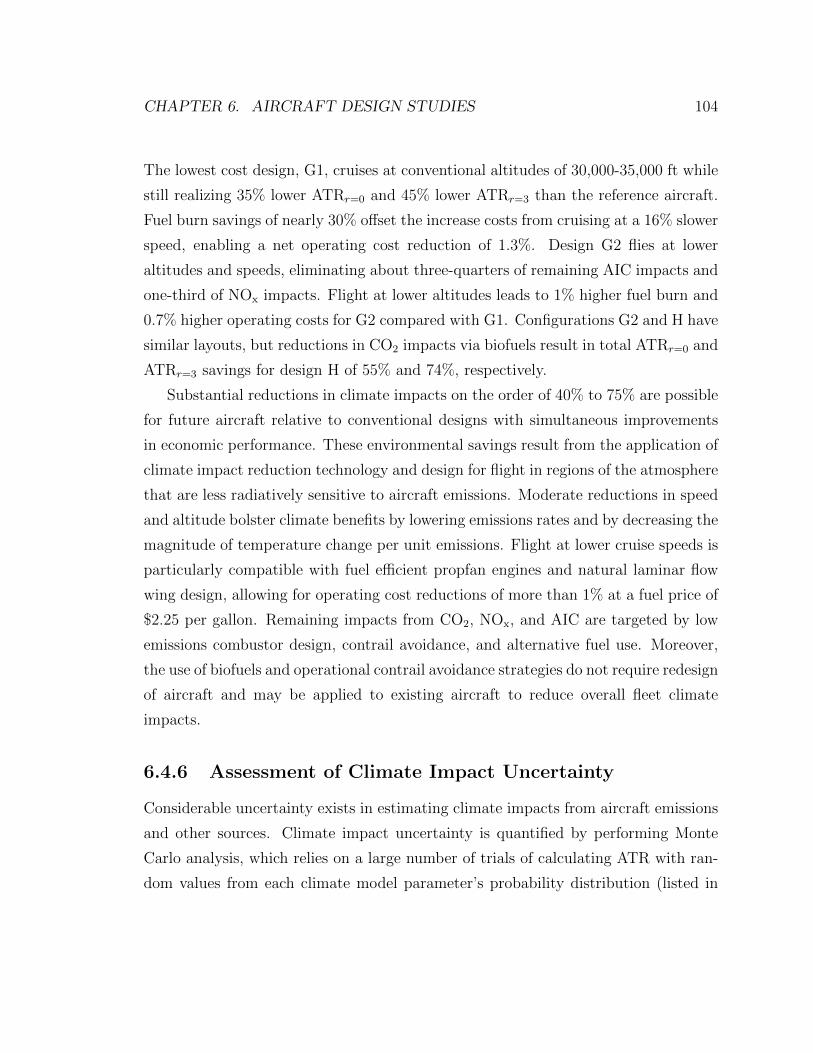
CHAPTER 6. AIRCRAFT DESIGN STUDIES 104
The lowest cost design, G1, cruises at conventional altitudes of 30,000-35,000 ft while
still realizing 35% lower ATRr=0 and 45% lower ATRr=3 than the reference aircraft.
Fuel burn savings of nearly 30% offset the increase costs from cruising at a 16% slower
speed, enabling a net operating cost reduction of 1.3%. Design G2 flies at lower
altitudes and speeds, eliminating about three-quarters of remaining AIC impacts and
one-third of NOx impacts. Flight at lower altitudes leads to 1% higher fuel burn and
0.7% higher operating costs for G2 compared with G1. Configurations G2 and H have
similar layouts, but reductions in CO2 impacts via biofuels result in total ATRr=0 and
ATRr=3 savings for design H of 55% and 74%, respectively.
Substantial reductions in climate impacts on the order of 40% to 75% are possible
for future aircraft relative to conventional designs with simultaneous improvements
in economic performance. These environmental savings result from the application of
climate impact reduction technology and design for flight in regions of the atmosphere
that are less radiatively sensitive to aircraft emissions. Moderate reductions in speed
and altitude bolster climate benefits by lowering emissions rates and by decreasing the
magnitude of temperature change per unit emissions. Flight at lower cruise speeds is
particularly compatible with fuel efficient propfan engines and natural laminar flow
wing design, allowing for operating cost reductions of more than 1% at a fuel price of
$2.25 per gallon. Remaining impacts from CO2, NOx, and AIC are targeted by low
emissions combustor design, contrail avoidance, and alternative fuel use. Moreover,
the use of biofuels and operational contrail avoidance strategies do not require redesign
of aircraft and may be applied to existing aircraft to reduce overall fleet climate
impacts.
6.4.6 Assessment of Climate Impact Uncertainty
Considerable uncertainty exists in estimating climate impacts from aircraft emissions
and other sources. Climate impact uncertainty is quantified by performing Monte
Carlo analysis, which relies on a large number of trials of calculating ATR with ran-
dom values from each climate model parameter’s probability distribution (listed in

CHAPTER 6. AIRCRAFT DESIGN STUDIES 105
A1 G1 G2 H
baseline combined combined added biojettechnology technologies technologies fuels
Maximum TOW [lbs] 161,600 151,000 146,100 146,100
Typical mission TOW [lbs] 140,600 137,500 134,400 134,400
Wing area [ft2] 1520 1610 1520 1520
Wing aspect ratio 8.9 14.9 16.9 16.8
Wing sweep [degrees] 34.0 7.0 7.0 7.0
Cruise Mach number 0.835 0.690 0.632 0.633
Initial cruise altitude [ft] 38,600 30,000 21,300 21,300
Final cruise altitude [ft] 39,800 34,900 29,200 29,100
SLS thrust [lbs] 23,200 22,300 20,900 21,000
Engine bypass ratio 8.4 60 60 60
Avg. cruise velocity [kts] 478 402 379 380
Normalized TOC 1.0000 0.9871 0.9941 1.0027
Normalized Wfuel 1.000 0.714 0.726 0.728
Normalized ENOx1.000 0.375 0.380 0.383
Cruise EINOx [g/kg] 19.8 10.4 10.3 10.3
O3 forcing factor 1.48 0.99 0.71 0.70
CH4 forcing factor 1.13 0.96 0.94 0.94
AIC forcing factor 0.80 1.37 0.34 0.33
Normalized ATRr=0 1.000 0.646 0.524 0.453
Fraction of ATRr=0 fromCO2/NOx/AIC [%]
65/17/17 72/5/22 91/2/7 89/2/8
Normalized ATRr=3 1.000 0.555 0.287 0.261
Fraction of ATRr=3 fromCO2 / NOx / AIC [%]
24/41/34 30/15/53 59/12/25 56/13/28
Table 6.6: Description of aircraft designed for minimum total operating costs andATRr=0 with multiple climate impact reduction technologies.
Chapter 5). A sufficient number of trials are computed so that the output distribu-
tions converge. All model parameters and forcing factor functions are assumed to be
uncertain except the climate sensitivity parameter S, applied in equation (5.15). This
parameter is simply a scaling factor that is applied to all calculations of ATR and its
uncertainty is not relevant for comparing relative impacts of different designs. For

CHAPTER 6. AIRCRAFT DESIGN STUDIES 106
each Monte Carlo trial, ATR is calculated for all designs using the same set of random
model parameter values. From the Monte Carlo analysis, the probability distribution
of the reduction in average temperature response, ATRref - ATR, is examined. By
quantifying the uncertainty in the ATR reduction of each design as opposed to the
uncertainty in the absolute ATR of each design, only the uncertainty relevant to the
differences between the designs is captured. Uncertainty in ATR reduction is more
appropriate for comparative study. For example, if two aircraft have identical fuel
burn and fly at identical altitudes but have different NOx emissions indices, the un-
certainty in ATR reduction between the two designs solely depends on uncertainty
in components of the climate model related to NOx impacts. If, on the other hand,
the uncertainty in absolute ATR is examined, uncertainty in all components of the
climate model (CO2, AIC, etc.) is included; a large portion of this uncertainty affects
both designs equally and is extraneous in a comparative study.
(a) (b)
Figure 6.10: Pareto front of normalized total operating cost and ATR, showing 66%confidence intervals for reduction in ATR relative to the reference design.
Figure 6.10 shows 66% likelihood ranges for reductions in ATR relative to the
reference aircraft, design A1. The pareto curves shown on this figure are identical
to those shown in Figure 6.9. Uncertainty ranges for each design reflect scientific
CHAPTER 6. AIRCRAFT DESIGN STUDIES 107
uncertainty in evaluating climate impacts and do not include uncertainty in estimating
aircraft performance. These 66% likelihood ranges are not symmetric about the best
estimate values. Instead, very large ATR reductions are more probable than very
small reductions. This is the case because the most significant differences between
the reference and low climate impact configurations lie in NOx and AIC impacts;
the radiative forcing parameters for both of these effects are lognormally distributed,
which leads to higher probability of large savings for lower altitude flight.
Beginning with the baseline technology scenario, ATR reduction uncertainty is
small for lowest cost designs because these configurations are fundamentally similar
to the reference aircraft. For baseline designs flying at lower altitudes, ATR re-
duction uncertainty increases substantially since low altitude configurations achieve
ATR savings by reducing impacts from NOx and AIC effects, which are highly un-
certain. Since ATRr=3 applies heavier weighting to less certain, short-lived impacts,
uncertainty is greater for ATRr=3 than ATRr=0. Nonetheless, the baseline technology
shaded region for nearly all designs remains below the unity ATR line, indicating that
there is at least an 83% confidence that these aircraft perform with lower ATR than
the reference aircraft. Uncertainty ranges for configurations using reduced climate
impact technologies are slightly wider. However, because these designs have lower
best estimate ATRs, there is greater confidence that they achieve significant climate
impact reductions relative to the reference aircraft. Figure 6.10 demonstrates that
scientific uncertainty is not too large to make conclusions about the relative climate
performance of competing designs.
Probability distributions for most climate model parameters are based on analy-
ses and expert opinions from climate modeling literature. For parameters where this
information is not available, probability distributions are inferred from the results
of multiple global climate model studies. Changes in the assumed distributions of
individual parameters would alter probability distributions in ATR reductions. For
example, beta or normal distributions could be assumed for each parameter. Beta
and uniform probability distributions are each bounded on both sides, unlike the nor-
mal and lognormal distributions applied here, which are bounded on zero and one
side, respectively. If beta distributions were applied, moderately narrower uncertainty

CHAPTER 6. AIRCRAFT DESIGN STUDIES 108
ranges in ATR reductions would be expected due to the additional domain bounding.
Similarly, significantly wider uncertainty ranges for climate model outputs would be
expected using uniform distributions (unless restrictive bounds are applied). It should
be noted, however, that with current scientific understanding, climate model parame-
ters are most appropriately described by normal and lognormal distributions because
of their unboundedness and because higher probabilities are assigned to parameter
values close to best estimates.
Next, the effect of the background CO2 scenario uncertainty is considered. As
noted before, the CO2 radiative forcing model used here assumes constant background
CO2 concentrations of 378 ppmv. However, it is likely that concentrations will vary
and exceed this value in the near-term. To assess this uncertainty, results from
the CO2 forcing models applied herein and in Ref. [53] are compared for aircraft
climate impacts assessed in Ref. [73]. For the alternative model, background CO2
concentrations are taken from Table VIII of Ref. [53] for the years 2000 to 2100, with
stable concentrations after 2100 of 685 ppmv. With a devaluation rate of 3%, relative
ATR estimates from the constant and varying CO2 concentration models are nearly
identical. Differences of less than 0.3% are observed in relative ATR and fractional
CO2 contributions. Results differ more significantly with a devaluation rate of zero.
The relative ATRs of low climate impact designs are 4-10% lower when calculated
with varying background CO2 concentrations. The fractional contributions of CO2
are also lower with this alternative model. There are two observations worth noting
about these results. First, the assumed scenario for background CO2 concentrations is
much more important for zero devaluation rates because all CO2 far future impacts are
included. Secondly, the assumption of varying background concentrations diminishes
the impacts of future aircraft CO2 emissions (only in the case of r = 0) because
as background concentrations increase, each unit of CO2 emissions causes a smaller
fractional increase in atmospheric CO2.

CHAPTER 6. AIRCRAFT DESIGN STUDIES 109
6.5 Alternative Metrics
Thus far, climate performance has been measured by the average temperature re-
sponse metric, developed for use in aircraft design studies. However, many other
climate metrics have been suggested for use in studies of impacts from aviation and
other sectors. This section addresses the extent to which choice of metric affects
conclusions about low climate impact aircraft design.
6.5.1 Comparison to Results with CO2-Based Metric
Some proposed metrics rely exclusively on CO2 emissions and are similar to fuel
consumption metrics. For example, ICAO’s Committee on Aviation Environmental
Protection is pursuing a CO2 emissions standard for future aircraft.[23] With CO2-
based metrics, the impacts of NOx emissions and AIC effects are either excluded or
modeled through a simple CO2 emissions scaling factor. One hundred year pulse
global temperature potential-based metrics are effectively similar to CO2-based met-
rics because only the impacts of CO2 emissions are experienced long after emissions
cease, as demonstrated in Ref. [123].
Figure 6.11 shows optimization results for aircraft designed to minimize CO2 emis-
sions and operating costs with varying technologies. These designs’ climate impacts as
measured by ATRr=0 and ATRr=3 are also plotted. Propfan, laminar flow, and biofuel
technologies are applied to these designs to reduce CO2 impacts. Strictly speaking,
low NOx combustor application would not be encouraged by CO2-based climate stan-
dards; however, it is possible that future improvements in emissions performance will
be mandated by more stringent landing and takeoff emissions standards, so the effects
of ultra low NOx combustors are also included. Burning extra fuel to operationally
avoid contrail formation would be disincentivized within a CO2 metric framework,
so this strategy is not included. For the baseline technology scenario, reductions in
CO2 emissions of up to 12% are achieved, translating into 2-5% lower ATRr=0 and
2-5% higher ATRr=3, similar to the minimum fuel burn design described in Table 6.3.
Fuel burn savings do not directly scale with ATR savings because of the sensitivity
of NOx and AIC impacts to changes in cruise altitude. By applying propfan engines,

CHAPTER 6. AIRCRAFT DESIGN STUDIES 110
laminar flow, low emissions combustors, and biojet fuel, CO2 emissions savings of up
to nearly 50% are possible. Measuring climate impacts instead with ATR, savings
drop to 20-30%, depending on the metric devaluation rate. These aircraft cruise at
altitudes of 30,000-36,000 ft where CO2 impacts are minimized, but NOx impacts are
high and AIC impacts are maximized. To compare, aircraft designed to minimize
ATR perform with 40-60% lower ATRr=0 and 50-85% lower ATRr=3 relative to the
same reference aircraft. These greater ATR savings are achieved through moderate
changes to design cruise altitude and application of a contrail avoidance strategy.
These results demonstrate the disparity in climate impact performance between
aircraft designed to minimize CO2 emissions and those designed for minimal temper-
ature change from all emissions. It is possible that if aircraft are designed exclusively
to reduce CO2 emissions, temperature change from NOx emissions and aviation in-
duced cloudiness may increase, offsetting some of the benefits of reduced carbon.
Significantly lower lifetime average temperature change can be achieved by consider-
ing impacts from non-CO2 emissions during the design and operation of an aircraft.
However, it should be noted that these temperature change impacts occur over very
different timescales, with a fraction of CO2-induced temperature change remaining in
the atmosphere for hundreds of years and NOx-induced and AIC-induced temperature
change decaying decades after emissions end.
6.5.2 Comparison to Results with Other Metrics
Average temperature response is proposed as a climate metric for the application
of aircraft design. However, other metrics could be developed to serve the same
purpose, as discussed in Chapter 3. Such alternative metrics include average radiative
forcing response (analogous to average temperature response) and 30 year sustained
temperature change. Each of these metrics quantifies the overall lifetime impacts from
all emissions released during the operation of a particular aircraft. Varying the metric
or the weighting function effectively adjusts the relative importance of long-lived CO2
emissions versus shorter-lived effects. Furthermore, metrics that are less appropriate
for aircraft design studies could also be considered: examples include radiative forcing,
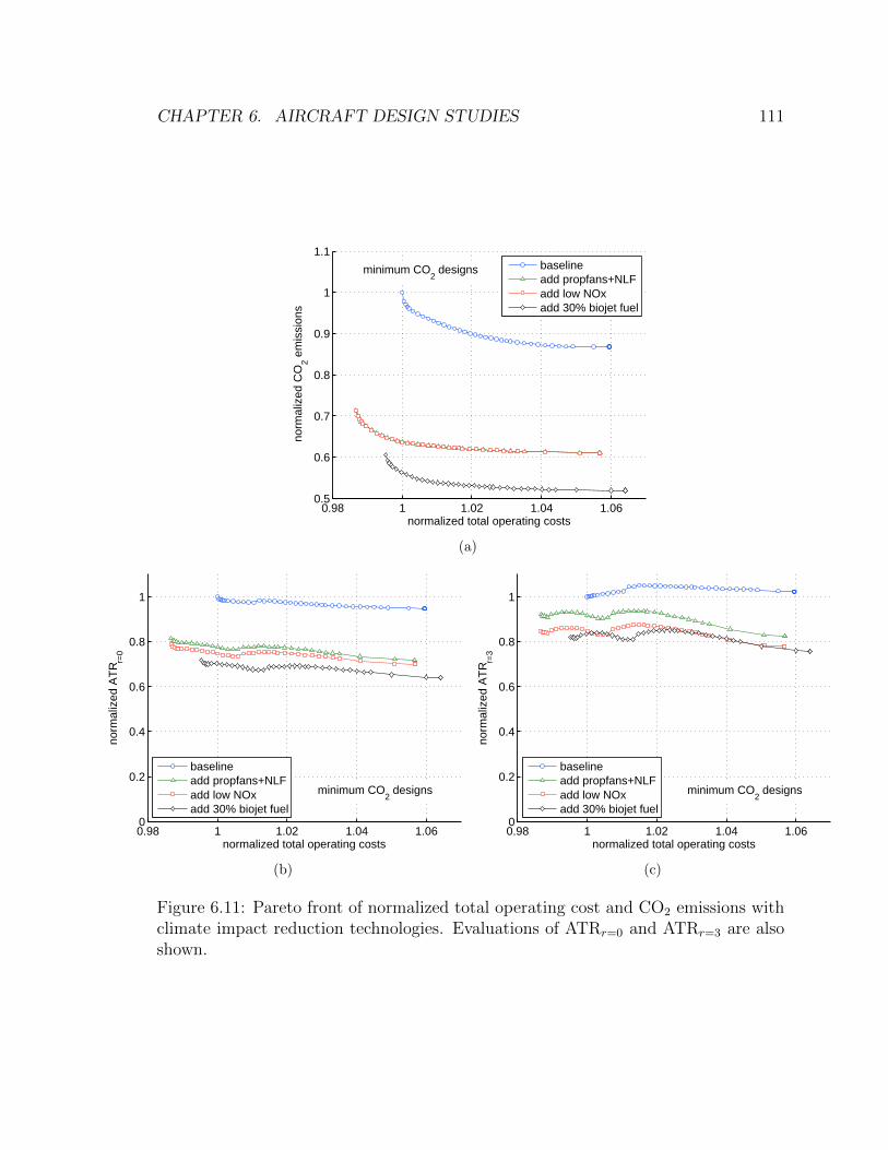
CHAPTER 6. AIRCRAFT DESIGN STUDIES 111
0.98 1 1.02 1.04 1.060.5
0.6
0.7
0.8
0.9
1
1.1
normalized total operating costs
norm
aliz
ed C
O2 e
mis
sion
s
minimum CO2 designs baseline
add propfans+NLFadd low NOxadd 30% biojet fuel
(a)
0.98 1 1.02 1.04 1.060
0.2
0.4
0.6
0.8
1
normalized total operating costs
norm
aliz
ed A
TR
r=0
minimum CO2 designs
baselineadd propfans+NLFadd low NOxadd 30% biojet fuel
(b)
0.98 1 1.02 1.04 1.060
0.2
0.4
0.6
0.8
1
normalized total operating costs
norm
aliz
ed A
TR
r=3
minimum CO2 designs
baselineadd propfans+NLFadd low NOxadd 30% biojet fuel
(c)
Figure 6.11: Pareto front of normalized total operating cost and CO2 emissions withclimate impact reduction technologies. Evaluations of ATRr=0 and ATRr=3 are alsoshown.

CHAPTER 6. AIRCRAFT DESIGN STUDIES 112
temperature change, or damage metrics based on past aviation impacts (e.g., scaling
RF in 2005 based on new emissions rates) or future emissions scenarios that poorly
represent the likely operation of a new aircraft (e.g., 100 year sustained global warming
or temperature potentials). Varying the choice of metric and its weighting function
causes changes in the magnitude of potential climate impact reductions. However, the
conclusions about strategies and design methods to reduce climate impacts remain
the same, except near the limiting case of metrics that exclude non-CO2 impacts
or model these effects by scaling CO2 emissions (e.g., CO2 metrics and long period
pulse global warming or temperature potentials), as explored in section 6.5.1. These
findings are demonstrated in Ref. [73] and illustrated by the similarities in Figures
6.1(a) and 6.1(b).
6.6 Additional Studies
The effects of climate model uncertainty are addressed in section 6.4.6. However,
other assumptions also impact aircraft performance predictions, and in particular
total operating cost estimates. This section explores the effect of fuel price and
mission range assumptions on the design tradeoff between operating costs and climate
impacts.
6.6.1 Effect of Varying Fuel Prices
Fuel prices are extremely volatile, so predictions of future prices are speculative.
Additionally, operating costs are sensitive to fuel price, affecting the balance between
requirements for short flight times and low fuel consumption for cost effective aircraft.
As fuel prices increase, technologies and strategies aimed at reducing fuel burn become
more economical. Thus, fuel price affects the economic competitiveness of reduced
climate impact aircraft. The tradeoffs between operating costs and climate impacts
are evaluated under two alternative fuel price scenarios: $1.50 per gallon and $3.50
per gallon, representative of the lowest and highest quarterly average aviation fuel
prices since 2005.[151] Optimization results are shown in Figure 6.12.
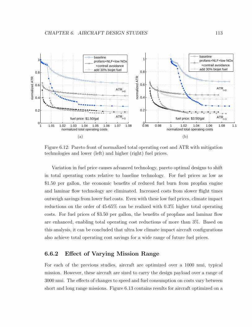
CHAPTER 6. AIRCRAFT DESIGN STUDIES 113
1 1.01 1.02 1.03 1.04 1.05 1.06 1.07 1.080
0.2
0.4
0.6
0.8
1
normalized total operating costs
norm
aliz
ed A
TR
fuel price: $1.50/galATR
r=3
ATRr=0
baselineprofans+NLF+low NOx +contrail avoidanceadd 30% biojet fuel
(a)
0.96 0.98 1 1.02 1.04 1.06 1.08 1.10
0.2
0.4
0.6
0.8
1
normalized total operating costs
norm
aliz
ed A
TR
fuel price: $3.50/gal ATRr=3
ATRr=0
baselineprofans+NLF+low NOx +contrail avoidanceadd 30% biojet fuel
(b)
Figure 6.12: Pareto front of normalized total operating cost and ATR with mitigationtechnologies and lower (left) and higher (right) fuel prices.
Variation in fuel price causes advanced technology, pareto optimal designs to shift
in total operating costs relative to baseline technology. For fuel prices as low as
$1.50 per gallon, the economic benefits of reduced fuel burn from propfan engine
and laminar flow technology are eliminated. Increased costs from slower flight times
outweigh savings from lower fuel costs. Even with these low fuel prices, climate impact
reductions on the order of 45-65% can be realized with 0.3% higher total operating
costs. For fuel prices of $3.50 per gallon, the benefits of propfans and laminar flow
are enhanced, enabling total operating cost reductions of more than 3%. Based on
this analysis, it can be concluded that ultra low climate impact aircraft configurations
also achieve total operating cost savings for a wide range of future fuel prices.
6.6.2 Effect of Varying Mission Range
For each of the previous studies, aircraft are optimized over a 1000 nmi, typical
mission. However, these aircraft are sized to carry the design payload over a range of
3000 nmi. The effects of changes to speed and fuel consumption on costs vary between
short and long range missions. Figure 6.13 contains results for aircraft optimized on a

CHAPTER 6. AIRCRAFT DESIGN STUDIES 114
longer range, 2800 nmi mission. Improvements in fuel efficiency from propfan engines
and laminar flow enable similar operating cost reductions for short and longer range
missions. However, operating costs are more sensitive to changes in design cruise
altitude on longer range missions, indicated by the difference in pareto curve slope
for low cost designs. As a result, aircraft flying at very low altitudes have worse
economic performance during longer range missions. Nonetheless, with advanced
technology and moderate altitude changes, ATRr=0 and ATRr=3 reductions of 50%
and 70% are possible with 1% lower operating costs than the reference, baseline
aircraft for short and medium range missions.
0.98 1 1.02 1.04 1.06 1.080
0.2
0.4
0.6
0.8
1
normalized total operating costs
norm
aliz
ed A
TR
r=0
long range mission
baselineadd propfan enginesadd laminar flowadd contrail avoidanceadd low NOx combustoradd 30% biojet fuel
(a)
0.98 1 1.02 1.04 1.06 1.080
0.2
0.4
0.6
0.8
1
normalized total operating costs
norm
aliz
ed A
TR
r=3
long range mission
baselineadd propfan enginesadd laminar flowadd contrail avoidanceadd low NOx combustoradd 30% biojet fuel
(b)
Figure 6.13: Pareto front of normalized total operating cost and ATR with designsoptimized over a long range mission.
6.7 Mitigation Strategies for Existing Aircraft
This chapter focuses on methods to reduce climate impacts of future aircraft. But
because commercial aircraft have long operating lifetimes, many aircraft flying today
will still be operating in 20 years.[3] To substantially improve climate performance of
the entire fleet, mitigation strategies for both new and existing aircraft are necessary.

CHAPTER 6. AIRCRAFT DESIGN STUDIES 115
Several of the strategies investigated for future aircraft are also applicable to existing
aircraft, including cruise altitude adjustments, operational contrail avoidance, and use
of biojet fuels. Relative performance impacts of mitigation strategies are estimated by
assessing the cost-climate impact tradeoff for a fixed geometry, conventional aircraft.
In the optimization, only cruise speed, altitudes, and typical mission takeoff weight are
allowed to vary, and the configuration layout is based on the reference, minimum cost
design A1. Figure 6.14 shows optimization results for cumulative application of these
strategies, noting that each point on a fixed design curve represents configuration A1,
operated at a different speed and altitude. For clarity, the baseline pareto curve of
new designs is also shown where each point represents a different configuration with
unique design parameters.
1 1.01 1.02 1.03 1.04 1.050
0.2
0.4
0.6
0.8
1
normalized total operating costs
norm
aliz
ed A
TR
r=0
new aircraft: baselinefixed design: baselinefixed design: contrail avoidancefixed design: add 30% biojet
(a)
1 1.01 1.02 1.03 1.04 1.050
0.2
0.4
0.6
0.8
1
normalized total operating costs
norm
aliz
ed A
TR
r=3
new aircraft: baselinefixed design: baselinefixed design: contrail avoidancefixed design: add 30% biojet
(b)
Figure 6.14: Pareto front of normalized total operating cost and ATR for designswith fixed configuration parameters representing conventional aircraft in the currentfleet.
Nearly equal climate benefits from reduced speed and altitude can be achieved
by conventional, existing aircraft compared with newly designed aircraft. However,
such climate savings for existing aircraft are associated with larger fuel and operating
cost penalties. An aircraft designed for lower speed flight can use a wing with lower
sweep and higher aspect ratio, but a fixed geometry aircraft flying at slower speeds

CHAPTER 6. AIRCRAFT DESIGN STUDIES 116
cannot benefit from these weight and drag savings. Additionally, the fixed geometry
conventional aircraft has a very large wing, leading to low, less aerodynamically ef-
ficient lift coefficients at reduced altitudes, unlike aircraft designed for low altitude
flight that employ smaller wings. It should also be noted that operating an existing
aircraft away from intended cruise altitudes increases fuel burn, thereby decreasing
maximum range. For instance, operating design A1 at Mach 0.80 and altitudes of
24,000-31,000 ft limits maximum range to 2600 nmi (while at the same time reducing
typical mission ATRr=0 and ATRr=3 by 10% and 33%, respectively). The adoption of
operational contrail avoidance and biofuels enables large reductions of at least 20% in
ATRr=0 and ATRr=3 at conventional cruise altitudes, similar to the benefits realized
by newly designed aircraft. In total, the combination of these strategies allows for
significant improvements in climate performance of existing aircraft, but the associ-
ated cost penalties are approximately twice as high as those for new aircraft with
comparable technology adoption.
Chapter 7
Conclusions and Future Work
7.1 Conclusions
The objective of this research was to develop a framework for assessing the compar-
ative climate impacts of different aircraft during conceptual design studies. Aircraft
emit numerous radiatively active species, each affecting the atmosphere over different
timescales. A linear climate model encompassing each of these effects and appropri-
ate for initial aircraft design studies was presented. This model accounted for the
variation in magnitudes of NOx and aviation induced cloudiness radiative forcings as
functions of emissions altitude. Design cruise altitude additionally affects aircraft fuel
consumption and NOx emission rates, and these dependencies were modeled simul-
taneously by integrating the climate model into an aircraft design and performance
estimation tool. The average temperature response metric was developed to mean-
ingfully quantify an aircraft’s lifetime operating climate change impacts. Lastly, the
uncertainty of individual model parameters was assessed to determine the level of
confidence in estimates of relative climate performance between competing aircraft
configurations.
Applying this framework, aircraft climate impact mitigation strategies were in-
vestigated. The powerful effect of design cruise altitude on climate impacts was
demonstrated, showcasing the potential for net climate impact reductions of 10-35%
by designing aircraft to fly at Mach 0.77 and 25,000-31,000 ft altitude (with 1% higher
117

CHAPTER 7. CONCLUSIONS AND FUTURE WORK 118
operating costs) when compared with more conventional designs that cruise at Mach
0.84, 39,000-40,000 ft altitude. The performance effects of climate impact reduction
technologies were modeled, including adoption of propfan engines, design for natural
laminar flow, replacement of conventional fuels with biofuels, use of low NOx combus-
tors, and development of an operational contrail avoidance strategy. Aircraft flying
below fuel-optimal altitudes incurred a fuel burn penalty, but propfan and laminar
flow technologies were applied to offset these penalties and produce large fuel savings.
Combining the effects of all technologies, climate impact savings on the order of 45%
in ATRr=0 and 70% in ATRr=3 were predicted along with total operating cost sav-
ings of 0.6% relative to a conventional, baseline technology, minimum cost aircraft.
Greater ATR reductions of 55% and 74% were predicted by applying biofuels, but
these designs were penalized by higher fuel prices.
Large uncertainties exist in estimating the climate impacts of aircraft. An uncer-
tainty quantification study was performed, which revealed that this scientific uncer-
tainty is not too great to make conclusions about the relative climate performance of
competing designs. Two-thirds likelihood ranges for ultra low climate impact designs
estimated ATRr=0 reductions of 28-75% (best estimate 46%) and ATRr=3 reductions
of 31-131% (best estimate 68%) relative to the reference aircraft. A separate source
of uncertainty in this study related to fuel prices. The economic benefits of low fuel
burn technologies, including propfan engines and natural laminar flow, were sensitive
to variation in fuel prices. However, the financial benefits of these technologies were
shown to be robust to these sensitivities: low climate impact configurations with mul-
tiple technologies achieved lower operating costs than a conventional, minimum cost
aircraft with baseline technology for fuel price scenarios of approximately $1.60 per
gallon and higher.
In this study, climate impacts were measured by the average temperature re-
sponse metric, developed for the application of comparative aircraft design studies.
This metric assessed the integrated, total temperature change produced by operation
of a particular aircraft. If instead, aircraft were designed to minimize CO2 emissions,
CO2 reductions of up to 45% are possible. However, because the effects of NOx and
CHAPTER 7. CONCLUSIONS AND FUTURE WORK 119
AIC were excluded from design consideration, maximum ATRr=0 and ATRr=3 reduc-
tions were limited to 30% and 20%, respectively. Comparable technology low ATR
designs achieved reductions of 50% and 75%, respectively, through design consider-
ation of non-CO2 impacts and application of operational contrail avoidance. These
results illustrated the importance of including non-CO2 emissions in an aircraft cli-
mate metric.
Finally, this research focused on the design of new aircraft. However, since com-
mercial aircraft have long operating lifetimes on the order of 30 years, reductions in
climate impacts from existing aircraft were necessary to improve fleetwide climate
performance. By flying existing aircraft at cruise altitudes that were less radiatively
sensitive and applying operational contrail avoidance and alternative fuels, ATRr=0
and ATRr=3 reductions of up to 20-30% and 40-60% were realized, with associated
operating cost increases of 2-5%. Thus, while significant climate impact reductions
were possible with existing aircraft, the economic penalties were much greater than
those for new reduced climate impact designs.
7.2 Future Work
This research established a framework for assessing the climate impacts of future air-
craft and quantified the climate benefits and economic impacts of various mitigation
strategies. A number of research opportunities exist to continue this work.
One area with potential for research advancement involves linear climate model de-
velopment. Further studies of aircraft climate impacts, most notably aviation induced
cloudiness, are needed to improve the accuracy of conceptual design climate models.
The AIC radiative forcing parameterization can be updated to include sensitivities to
engine exhaust temperature and water content. Furthermore, forcing factors devel-
oped for this research were based on results from a single global climate model study.
Additional global climate model studies are necessary to improve understanding of
the variation in NOx and AIC radiative forcings with altitude, and additionally, lat-
itude. Similarly, the diurnal and seasonal variation in AIC forcing factors could be

CHAPTER 7. CONCLUSIONS AND FUTURE WORK 120
quantified. With these model advancements, climate assessments can be performed
over more realistic time-dependent and three-dimensional flight routings.
This research revealed an opportunity for significant aircraft climate impact re-
ductions via design cruise altitude changes. However, it is likely that aircraft flying at
lower altitudes will encounter more turbulence, affecting cruise wing loading, airframe
maintenance, and passenger comfort. Operating many aircraft in the 25,000-30,000
altitude band may also lead to increased airspace congestion. More research is needed
to investigate the effects of operating both existing and future aircraft at moderately
lower cruise altitudes compared with conventional commercial fleet routing.
A mitigation strategy assessed here was operational contrail avoidance, first pro-
posed by Mannstein et al.[147] For this strategy to be viable, advancements in hu-
midity sensors, weather forecasting, and flight planning are necessary. Further in-
vestigation of the horizontal extent of contrailing ice-supersaturated layers is needed
to determine the feasibility of this operational strategy. In particular, if individual
CISSLs are too small in horizontal scope or if the height of a typical CISSL meanders
horizontally, meaning that its average altitude varies by thousands of feet within its
horizontal extent, then the model of contrail avoidance through a single ±2000-4000
ft shift may not be sufficient to reduce AIC impacts. Additionally, future research
should consider how this type of strategy can be integrated into air traffic manage-
ment systems without exceeding realistic traffic congestion and controller workload
limits.
The benefits of low NOx combustors were estimated in this research based on
simple technology factors. Future advanced technology combustor design will likely
involve tradeoffs between emission rates of NOx and other species, combustion effi-
ciency, and configuration weight. Higher fidelity, physics-based models are needed
to answer questions about combustor design for minimal operating costs and climate
impacts.
Estimates of operating costs in this research were based on current, typical airline
operating expenses. However, it is likely that in the next decade, taxes and regulations
could be introduced with the goal of limiting future aircraft climate change. As
demonstrated in Chapter 6, studies of aircraft designed to minimize CO2 emissions
CHAPTER 7. CONCLUSIONS AND FUTURE WORK 121
versus average temperature response yielded different climate performance levels and
solution strategies. Future studies could consider the impacts of proposed policy
changes on the conclusions of aircraft design studies.
Aircraft design studies in this research were limited to conventional fuels and
tube-wing configurations. Applying climate impact reduction technologies to blended-
wing-body aircraft could enable further emissions and climate impact savings. These
configurations also provide community noise benefits through airframe shielding and
may be well-suited for propfan engine application. The conceptual design methods
applied here were derived for traditional configurations; assessment of unconventional
aircraft technologies requires the development of appropriate conceptual design and
performance methods.

Appendix A
Turbofan and Propfan
Performance Model
Performance of turbofan and propfan engines, including fuel consumption and avail-
able thrust, is estimated with a cycle analysis. In this analysis, the thermodynamic
properties of the flow are computed at each station in the engine based on energy rela-
tionships. The same cycle analysis is applied for both turbofan and propfan engines,
and differences between these configurations are modeled through engine design pa-
rameters and efficiencies. Fan efficiencies are predicted using simple propeller theory.
The cycle analysis described herein is based on the methods presented in Refs.
[21, 90]. Key assumptions for this engine model are as follows:
• The flow is one-dimensional at each axial station.
• The flow is steady on average.
• The fluid behaves as a perfect gas with constant molecular weights and specific
heats both upstream and downstream of the burner.
• High pressure bleed air and engine cooling air are removed after the fluid exits
the high pressure compressor, but before the fluid enters the burner.
• Diffusers and nozzles are adiabatic.
122

APPENDIX A. TURBOFAN AND PROPFAN PERFORMANCE MODEL 123
• Fan, compressor, and turbine component performance are described by constant
polytropic efficiencies.
• Exhaust streams from the core and bypass ducts exit the engine through sepa-
rate convergent nozzles.
• There is no booster on the low pressure spool.
• Installation penalties are modeled as a constant fractional loss in thrust at all
operating conditions.
This cycle analysis models specific fuel consumption and available specific thrust
at all flight conditions and throttle settings for an engine with user-specified design
variables and component efficiencies. The result is a “rubber engine” whose thrust
can be adjusted by scaling mass flow rates.
Cycle Notation and Component Assumptions
Before describing the model equations, notation and engine station numbering are
established. Figure A.1 shows standard station numbering and mass flows for a two-
spool, separate exhaust engine. A low pressure spool connects the fan and low pressure
turbine, and a high pressure spool connects the high pressure compressor and turbine.
Station properties m, M , T , and P refer to mass flow, Mach number, temperature,
and pressure, respectively. The subscript T denotes a station stagnation property.
The variables τ and π indicate temperature and pressure ratios. Gas properties take
on constant but different values upstream and downstream of the burner. For all
stations upstream of station 3, the gas constant, specific heat, and ratio of specific
heats are denoted Rc, Cpc, and γc. Corresponding properties downstream of station 4
are given by Rt, Cpt, and γt. Key parameter relationships at each station are described
in the following sections.
Station 0: Far upstream of the engine entrance (not shown in the figure). The
total mass flow through the engine fan is m0. Ratios of stagnation to static properties

APPENDIX A. TURBOFAN AND PROPFAN PERFORMANCE MODEL 124
fan
H.P. compressor
burner coolant mixer #1
coolant mixer #2
H.P. turbine
L.P. turbine
core nozzle
bypass nozzle
19
13
2.5
3 3.1
4
4.1
4.4
4.5
5
9
2
high pressure spool
low pressure spool
bleed air
cooling air #2
cooling air #1
Figure A.1: Diagram of engine station numbering, adapted from Ref. [21].
are given by τr and πr.
τr =TT0
T0
= 1 +γc − 1
2M0
2 and πr =PT0
P0
= τrγcγc−1 (A.1)
Station 2b and 2c: Fan face. The bypass ratio, α, describes the fractions of total
mass flow entering the bypass and core streams. Prior to reaching the fan face, the
flow may pass through a diffuser. The diffuser is assumed to be adiabatic but not
isentropic due to wall friction. In some engines including the propfan, the diffusers
for the bypass and core streams may perform differently, so separate parameters are
necessary.
m2b =α
α + 1m0 and m2c =
1
α + 1m0 (A.2)
πdb =PT2b
PT0
and πdc =PT2c
PT0
(A.3)
Stations 13 and 2.5: Bypass and core stream fan exit. The stagnation pressure
ratio across the fan is an important design parameter for the engine. The stagnation

APPENDIX A. TURBOFAN AND PROPFAN PERFORMANCE MODEL 125
temperature ratio is related to fan pressure ratio through fan polytropic efficiency, ef ,
which prescribes the required power input from the low pressure spool to run the fan.
Because there are no booster stages on the low pressure spool, the fan pressure ratio
for the bypass and core streams are identical. Mass flow rates entering and exiting
the fan are equal, m13 = m2b and m2.5 = m2c.
πf =PT13
PT2b
=PT2.5
PT2c
and τf =TT13
TT2
=TT2.5
TT2
= πfγc−1γc ef (A.4)
Station 3: High pressure compressor exit. The stagnation pressure ratio across the
high pressure compressor is another key engine design parameter. Similarly to the
fan, the performance of the high pressure compressor is described by the compressor
polytropic efficiency, ech. Mass flow rates at the high pressure compressor entrance
and exit are identical, m3 = m2c.
πch =PT3
PT2.5
and τch =TT3
TT2.5
= πchγc−1γc ech (A.5)
Station 3.1: Burner entrance. Between the high pressure compressor exit and the
burner entrance, bleed and turbine cooling air are removed. δ1 and δ2 give cooling
air fractions, mci = δi m2c, and β represents the bleed air fraction. Thermodynamic
properties are unchanged.
m3.1 = (1− β − δ1 − δ2) m2c (A.6)
Station 4: Burner exit. The stagnation temperature at the burner exit, TT4, is a
key design variable for an aircraft engine. Increases in TT4 improve overall efficiency,
but this parameter is limited by material properties. Across the burner, stagnation
pressure drops due to viscous losses and heat addition. The fuel mass added to the
flow, mf is defined by the variable f .
f =mf
m3.1
and m4 = (1− β − δ1 − δ2) (1 + f) m2c (A.7)
πb =PT4
PT3.1
(A.8)

APPENDIX A. TURBOFAN AND PROPFAN PERFORMANCE MODEL 126
Station 4.1: First coolant mixer exit. Because burner exit temperatures often
approach or exceed the melting point of turbine blade materials, cooling flows are
necessary. In this coolant mixer, cooler air diverted upstream of the burner is mixed
with air exiting the combustor. The pressure change in this mixing process is not
modeled, and high pressure turbine polytropic efficiency is penalized to account for
the effects of cooling.[21]
m4.1 = [(1− β − δ1 − δ2) (1 + f) + δ1] m2c (A.9)
Station 4.4: High pressure turbine exit. In the high pressure turbine, power is
extracted from the flow to drive the high pressure compressor. The efficiency of this
process is described by the high pressure turbine polytropic efficiency, eth, which
relates the stagnation temperature and pressure ratios across the turbine. Mass flows
at the turbine entrance and exit are equal, m4.4 = m4.1.
τth =TT4.4
TT4.1
and πth =PT4.4
PT4.1
= τthγt
(γt−1) eth (A.10)
Station 4.5: Second coolant mixer exit. The first and second coolant mixers are
modeled similarly.
m4.5 = [(1− β − δ1 − δ2) (1 + f) + δ1 + δ2] m2c (A.11)
Station 5: Low pressure turbine exit. The low pressure turbine extracts power
from the flow to drive the fan. Again, the temperature and pressure ratios through
the turbine are related through the low pressure turbine polytropic efficiency, etl.
Mass flow rates at the turbine entrance and exit are equal, m5 = m4.5.
τtl =TT5
TT4.5
and πtl =PT5
PT4.5
= τtlγt
(γt−1) etl (A.12)
Stations 19 and 9: Core and bypass stream nozzle exit. Both nozzles are assumed
to be adiabatic but not isentropic due to wall friction. Nozzle performance is defined
by the stagnation pressure ratio. Core exhaust mass flow rate equals the turbine

APPENDIX A. TURBOFAN AND PROPFAN PERFORMANCE MODEL 127
exit flow, m9 = m4.5, and fan exhaust flow rate is the same as the fan face value,
m19 = m2c.
πnb =PT19
PT13
and πnc =PT9
PT5
(A.13)
Cycle Analyis
To perform the cycle analysis and solve for properties at each station, additional equa-
tions are introduced that describe how components function together. Five power bal-
ance equations relate stagnation temperatures at different stations. These equations
represent power balance across the burner (A.14), the high pressure spool (A.15), the
low pressure spool (A.16), and the two coolant mixers (A.17 and A.18). Mechanical
shaft efficiencies for the high pressure and low pressure spools, ηmh and ηml, represent
the ratios of power entering the shaft from the turbine to the power leaving the shaft
to the compressor. Burner efficiency, ηb, denotes the ratio of thermal energy increase
in the flow compared with the ideal energy change based on the fuel heating value,
hfuel.
m3.1Cpc TT3 + mf hfuel ηb = m4Cpt TT4 (A.14)
m4.1Cpt (TT4.1 − TT4.4) ηmh = m2.5Cpc (TT3 − TT2.5) (A.15)
m4.5Cpt (TT4.5 − TT5) ηml = m0Cpc (TT2.5 − TT2) (A.16)
mc1Cpc TT3 + m4Cpt TT4 = m4.1Cpt TT4.1 (A.17)
mc2Cpc TT3 + m4.4Cpt TT4.4 = m4.5Cpt TT4.5 (A.18)
After solving this system of equations, all station stagnation properties are known.
However, static conditions at the engine exhaust plane must also be found to deter-
mine thrust. Because both the core and fan bypass streams exit the engine through
convergent nozzles, flows at the exit planes may be choked. Exhaust plane conditions
are solved via equations (A.19) and (A.20), which enable calculation of M19 and M9
and hence V19 and V9.
PT19
P19
= min
[πr πdf πf πnf ,
γc + 1
2
γcγc−1]
; (A.19)
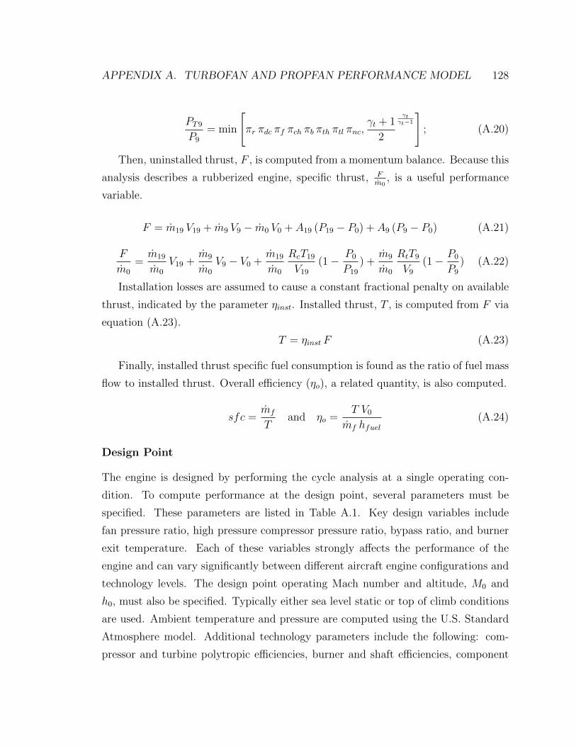
APPENDIX A. TURBOFAN AND PROPFAN PERFORMANCE MODEL 128
PT9
P9
= min
[πr πdc πf πch πb πth πtl πnc,
γt + 1
2
γtγt−1
]; (A.20)
Then, uninstalled thrust, F , is computed from a momentum balance. Because this
analysis describes a rubberized engine, specific thrust, Fm0
, is a useful performance
variable.
F = m19 V19 + m9 V9 − m0 V0 + A19 (P19 − P0) + A9 (P9 − P0) (A.21)
F
m0
=m19
m0
V19 +m9
m0
V9 − V0 +m19
m0
RcT19
V19
(1− P0
P19
) +m9
m0
RtT9
V9
(1− P0
P9
) (A.22)
Installation losses are assumed to cause a constant fractional penalty on available
thrust, indicated by the parameter ηinst. Installed thrust, T , is computed from F via
equation (A.23).
T = ηinst F (A.23)
Finally, installed thrust specific fuel consumption is found as the ratio of fuel mass
flow to installed thrust. Overall efficiency (ηo), a related quantity, is also computed.
sfc =mf
Tand ηo =
T V0
mf hfuel(A.24)
Design Point
The engine is designed by performing the cycle analysis at a single operating con-
dition. To compute performance at the design point, several parameters must be
specified. These parameters are listed in Table A.1. Key design variables include
fan pressure ratio, high pressure compressor pressure ratio, bypass ratio, and burner
exit temperature. Each of these variables strongly affects the performance of the
engine and can vary significantly between different aircraft engine configurations and
technology levels. The design point operating Mach number and altitude, M0 and
h0, must also be specified. Typically either sea level static or top of climb conditions
are used. Ambient temperature and pressure are computed using the U.S. Standard
Atmosphere model. Additional technology parameters include the following: com-
pressor and turbine polytropic efficiencies, burner and shaft efficiencies, component
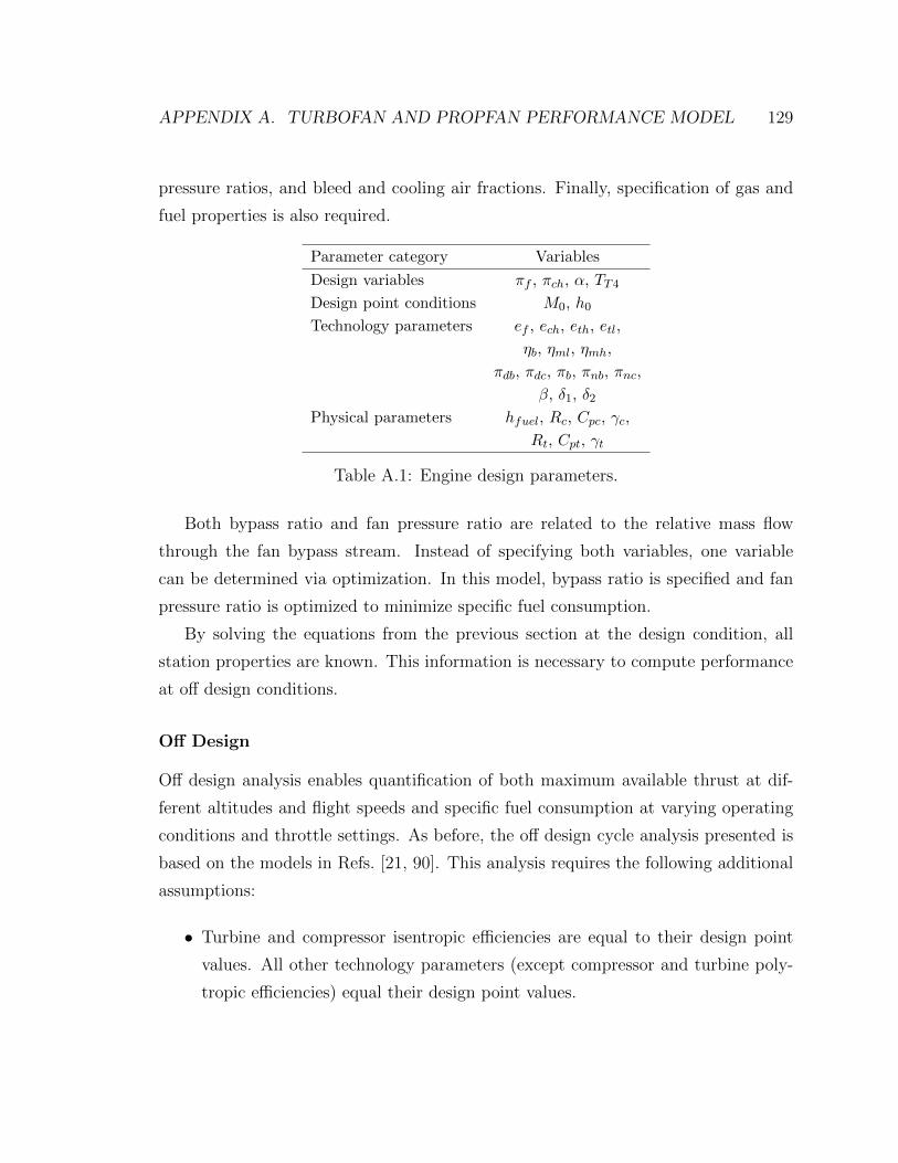
APPENDIX A. TURBOFAN AND PROPFAN PERFORMANCE MODEL 129
pressure ratios, and bleed and cooling air fractions. Finally, specification of gas and
fuel properties is also required.
Parameter category Variables
Design variables πf , πch, α, TT4
Design point conditions M0, h0
Technology parameters ef , ech, eth, etl,
ηb, ηml, ηmh,
πdb, πdc, πb, πnb, πnc,
β, δ1, δ2
Physical parameters hfuel, Rc, Cpc, γc,
Rt, Cpt, γt
Table A.1: Engine design parameters.
Both bypass ratio and fan pressure ratio are related to the relative mass flow
through the fan bypass stream. Instead of specifying both variables, one variable
can be determined via optimization. In this model, bypass ratio is specified and fan
pressure ratio is optimized to minimize specific fuel consumption.
By solving the equations from the previous section at the design condition, all
station properties are known. This information is necessary to compute performance
at off design conditions.
Off Design
Off design analysis enables quantification of both maximum available thrust at dif-
ferent altitudes and flight speeds and specific fuel consumption at varying operating
conditions and throttle settings. As before, the off design cycle analysis presented is
based on the models in Refs. [21, 90]. This analysis requires the following additional
assumptions:
• Turbine and compressor isentropic efficiencies are equal to their design point
values. All other technology parameters (except compressor and turbine poly-
tropic efficiencies) equal their design point values.

APPENDIX A. TURBOFAN AND PROPFAN PERFORMANCE MODEL 130
• The flow is choked at the entrances to both the high pressure and low pressure
turbines (stations 4.1 and 4.5).
• Maximum thrust at any operating condition is limited such that neither TT4
nor πch exceed their design point values.
To apply the first assumption, compressor and turbine polytropic efficiencies, ei,
must be converted into isentropic efficiencies, ηi, at the design point. The second
assumption introduces additional relationships between thermodynamic conditions
and design and off design conditions. These equations are described in Refs. [21, 90].
The resulting system of equations is nonlinear and must be solved numerically.
The third assumption establishes a simple engine control system that limits max-
imum thrust. In this model, high pressure compressor pressure ratio and burner
exit temperature are limited to not exceed their design point values. In a real en-
gine, other parameters such as shaft rotational speed, burner entry temperature, and
burner pressure are also controlled; however, πch and TT4 have the most dominant ef-
fect in limiting thrust.[90] Burner temperature can be scheduled to allow for different
maximum temperatures depending on operating conditions, but a single limit is used
for this simple model. Additionally, thrust for unducted engines is limited by max-
imum blade loading, effectively reducing available thrust at takeoff conditions. The
effect of engine throttling at a given flight altitude and speed is modeled by reducing
the burner exit temperature below its maximum value (which is limited by either
design TT4 or πch). Then, specific fuel consumption and thrust may be calculated for
partial throttle operation.
Fan Polytropic Efficiency
Engines with different bypass ratios can be driven by similar engine cores, with the
same core component efficiencies. However, the low pressure compressor system ef-
ficiencies of a moderate bypass ratio turbofan and a very high bypass ratio propfan
can differ significantly. In particular, low pressure spool mechanical efficiency, fan
diffuser and nozzle pressure ratios, and fan polytropic efficiency all vary depending

APPENDIX A. TURBOFAN AND PROPFAN PERFORMANCE MODEL 131
on the fan configuration. This section describes methods to quantify the variation in
fan polytropic efficiency with bypass ratio and fan layout.
Fan polytropic efficiency and propulsive efficiency, ef and ηprop, measure separate
quantities. Fan polytropic efficiency describes the entropy rise during compression;
propulsive efficiency, on the other hand, is the ratio of useful thrust power to input
shaft power. Propulsive efficiency includes axial induced momentum losses while fan
polytropic efficiency does not. The approximate relationship between these two effi-
ciencies is given by equation (A.25) as derived in Ref. [152]. The efficiency parameter
used in cycle analysis is ef , but ηprop is used more often in propfan design. In this
section, both efficiencies are computed.
ηprop ≈2V0
V0 + V19
ef (A.25)
Based on one-dimensional cycle analysis, fan specific thrust and power (excluding
the core) are related through fan pressure ratio and polytropic efficiency. This analysis
is intended to isolate efficiency losses in the fan, and no other losses are modeled.
Assuming a fully expanded exhaust and no pressure change in the nozzle and diffuser,
specific thrust and power are given by equations (A.26) and (A.27).
Ffanmfan
=
√2
γc − 1
(πf
γc−1γc − 1
)√γcRc T0 πf
γc−1γc
( 1ef−1) − V0 (A.26)
Pfanmfan
= Cpc T0 τr
(πf
γc−1γc ef − 1
)(A.27)
These one-dimensional equations can be combined with propeller analysis methods
to determine the polytropic efficiency of a fan with specified thrust based on losses
from drag and energy left in the wake. Separate propeller models are presented for
single rotation propellers, dual rotation propellers, and rotor-stator configurations.
The propeller analysis methods presented are very simple but capture the relative
differences in performance between fan designs.

APPENDIX A. TURBOFAN AND PROPFAN PERFORMANCE MODEL 132
Single Rotor The simplest fan configuration for a propfan engine is a single pro-
peller. Single propeller performance can be estimated with a combination of mo-
mentum, blade element and vortex theory as described by Glauert.[79] This classical
theory is developed for low disk loadings, but is also sufficient for preliminary per-
formance estimates in highly loaded propellers.[153] The related method presented
in Ref. [154] is applied for this analysis. This model designs an optimally loaded
propeller and computes thrust and efficiency, including losses from swirl, tip effects,
and viscous blade drag. With a single row of propeller blades, the swirl losses, or
rotational momentum left in the wake, can cause efficiency losses greater than 25%.
Because of this, single propeller configurations are only appropriate for relatively low
advance ratios. Depending on where the engines are installed on the aircraft, swirl
losses can be recovered through simultaneous propeller and wing design.[84, 92]
A diagram of velocities is given in Figure A.2. The propeller induces axial and
tangential velocities at the propeller face that are characterized by the dimensionless
quantities a = uaV0
and a′ = utΩr
. Circulation is denoted Γ, the number of blades B,
and the section drag-to-lift ratio ε. The net resultant force is resolved into thrust
in the axial direction and torque in the tangential direction. Thrust and torque per
unit radius, F ′ and Q′, are described by equations (A.28), (A.29), (A.30), and (A.31)
based on momentum and vortex models.
F ′ = 4π r ρ V02 a (1 + a) κ−B ε ρΓV0 (1 + a) (A.28)
F ′ = B ρΓ Ω r (1− a′)−B ε ρΓV0 (1 + a) (A.29)
Q′ = B ρΓV0 r (1 + a) +B ε ρΓ Ω r2 (1− a′) (A.30)
Q′ = 4π r2 ρ V0 Ω r (1 + a) a′ κ+B ε ρΓ Ω r2 (1− a′) (A.31)
In these equations, κ represents the Prandtl loss function, which accounts for mo-
mentum loss due to radial flow near the tips.[79] This function is defined in equation
(A.32).
κ =2
πcos−1
(exp
[−B (1− rR
)
2 sinφr=R
])where tanφ =
V0 (1 + a)
Ω r (1− a′)(A.32)
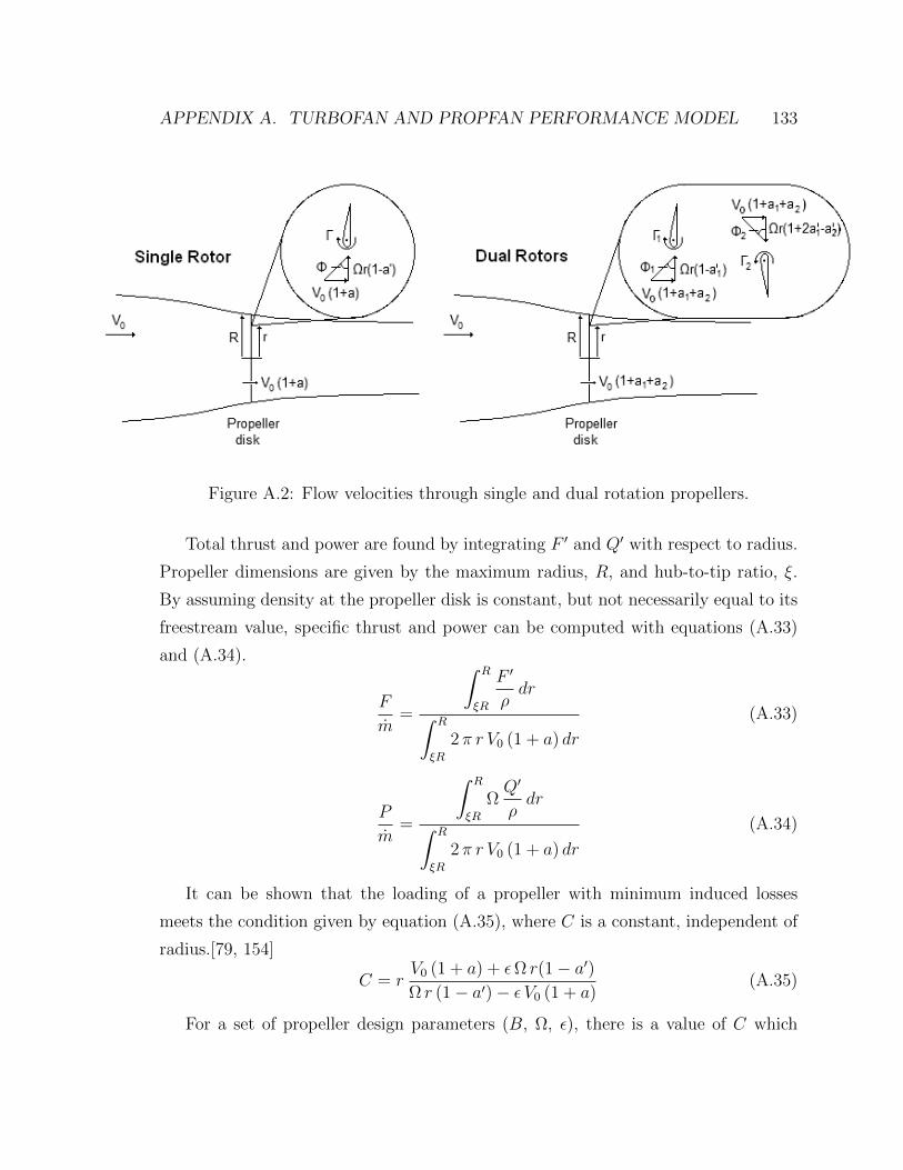
APPENDIX A. TURBOFAN AND PROPFAN PERFORMANCE MODEL 133
Figure A.2: Flow velocities through single and dual rotation propellers.
Total thrust and power are found by integrating F ′ and Q′ with respect to radius.
Propeller dimensions are given by the maximum radius, R, and hub-to-tip ratio, ξ.
By assuming density at the propeller disk is constant, but not necessarily equal to its
freestream value, specific thrust and power can be computed with equations (A.33)
and (A.34).
F
m=
∫ R
ξR
F ′
ρdr∫ R
ξR
2 π r V0 (1 + a) dr
(A.33)
P
m=
∫ R
ξR
ΩQ′
ρdr∫ R
ξR
2 π r V0 (1 + a) dr
(A.34)
It can be shown that the loading of a propeller with minimum induced losses
meets the condition given by equation (A.35), where C is a constant, independent of
radius.[79, 154]
C = rV0 (1 + a) + εΩ r(1− a′)Ω r (1− a′)− ε V0 (1 + a)
(A.35)
For a set of propeller design parameters (B, Ω, ε), there is a value of C which

APPENDIX A. TURBOFAN AND PROPFAN PERFORMANCE MODEL 134
corresponds to a given specific thrust requirement. The power consumed by the pro-
peller can also be computed, and fan polytropic efficiency is determined by combining
equations (A.27) and (A.34).
Dual Rotor Because swirl losses can be detrimental for heavily loaded propellers,
dual rotation propellers are sometimes desirable for open rotor configurations. In
a dual rotation propeller, or a counter-rotating propeller, two propellers rotate in
opposite directions around the same axis and are designed to reduce swirl losses.
Counter-rotating configurations also benefit from the partial cancellation of reaction
torques produced by the engines, reducing structural loading.[155]
The single propeller analysis is adapted for dual rotation propellers by applying
Lock’s assumptions about the induced velocities of counter-rotating propellers.[156]
These assumptions are repeated below.
• The interference velocities at any blade element may be calculated by consider-
ing the velocity fields of the two airscrews independently and adding the effects.
• Either airscrew produces its own interference velocity field which so far as it
affects the airscrew itself is exactly the same as if the other airscrew were absent
and includes the usual tip loss correction.
• Added to this is the velocity field of the other airscrew. Since the two are
rotating in opposite directions, the effect will be periodic and its time average
value may be taken to be equal to the average value round a circle having a
radius of the blade element.
Each rotor induces axial and tangential velocities, again denoted ai =ua,iV0
and
a′i =ut,iΩ1 r
, where subscripts 1 and 2 refer to the front and rear rotors, respectively.
This model further assumes that the rotors lie in the same plane, and the axial flow
velocities through the two propellers are identical and equal to V0(1 + a1 + a2). Each
rotor induces a dimensionless tangential velocity a′i on itself and a′j on the opposite
disk. Following Theodorsen, the tangential velocity behind the disk is twice its value
at the disk plane, and no tangential flow is induced ahead of the disk.[157]. Induced

APPENDIX A. TURBOFAN AND PROPFAN PERFORMANCE MODEL 135
tangential velocities at each disk are given by equation (A.36). Axial and tangential
velocities through each rotor are shown in Figure A.2.
i = 1
a′i = a′1
a′j = 0
i = 2
a′i = a′2
a′j = −2 a′1(A.36)
Applying the above assumptions to the combined vortex, blade element, and mo-
mentum theory for single propellers, equations (A.37)-(A.40) for thrust and torque
per unit radius on each rotor i are developed. Each rotor contains B blades.
F ′i = 4π r ρ V02 ai (1 + a1 + a2) κi −B εi ρΓi V0 (1 + a1 + a2) (A.37)
F ′i = B ρΓi Ω1 r
(Ωi
Ω1
− a′i − a′j)−B εi ρΓi V0 (1 + a1 + a2) (A.38)
Q′i = B ρΓi V0 r (1 + a1 + a2) +B εi ρΓi Ω1 r2
(Ωi
Ω1
− a′i − a′j)
(A.39)
Q′i = 4π r2 ρ V0 Ω1 r (1 + a1 + a2) a′i κi +B εi ρΓi Ω1 r2
(Ωi
Ω1
− a′i − a′j)
(A.40)
Momentum loss factors κ1 and κ2 are defined similarly to κ in the single propeller
case, where φi refers to the local flow angle at each rotor. Again assuming that the
density at each rotor disk is constant, the total thrust and power may be found by
integrating and summing thrust and torque per unit radius.
F
m=
∫ R
ξR
(F ′1 + F ′2
ρ
)dr∫ R
ξR
2 π r V0 (1 + a1 + a2) dr
(A.41)
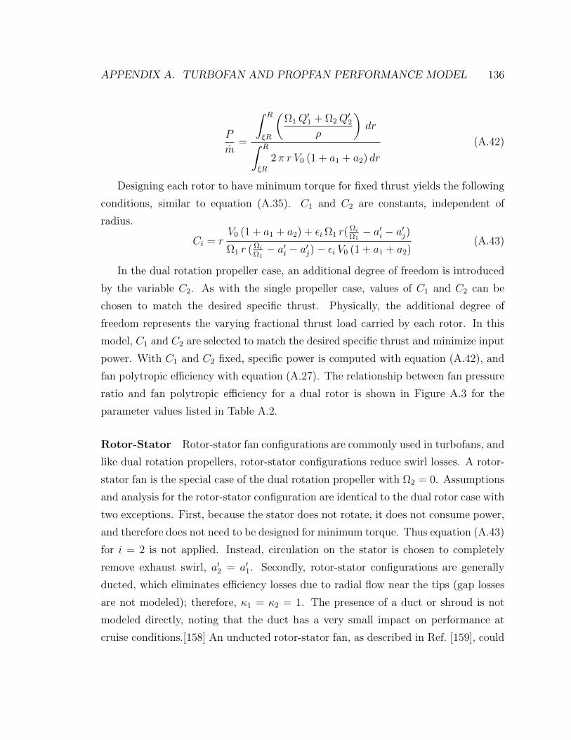
APPENDIX A. TURBOFAN AND PROPFAN PERFORMANCE MODEL 136
P
m=
∫ R
ξR
(Ω1Q
′1 + Ω2Q
′2
ρ
)dr∫ R
ξR
2 π r V0 (1 + a1 + a2) dr
(A.42)
Designing each rotor to have minimum torque for fixed thrust yields the following
conditions, similar to equation (A.35). C1 and C2 are constants, independent of
radius.
Ci = rV0 (1 + a1 + a2) + εi Ω1 r(
ΩiΩ1− a′i − a′j)
Ω1 r ( ΩiΩ1− a′i − a′j)− εi V0 (1 + a1 + a2)
(A.43)
In the dual rotation propeller case, an additional degree of freedom is introduced
by the variable C2. As with the single propeller case, values of C1 and C2 can be
chosen to match the desired specific thrust. Physically, the additional degree of
freedom represents the varying fractional thrust load carried by each rotor. In this
model, C1 and C2 are selected to match the desired specific thrust and minimize input
power. With C1 and C2 fixed, specific power is computed with equation (A.42), and
fan polytropic efficiency with equation (A.27). The relationship between fan pressure
ratio and fan polytropic efficiency for a dual rotor is shown in Figure A.3 for the
parameter values listed in Table A.2.
Rotor-Stator Rotor-stator fan configurations are commonly used in turbofans, and
like dual rotation propellers, rotor-stator configurations reduce swirl losses. A rotor-
stator fan is the special case of the dual rotation propeller with Ω2 = 0. Assumptions
and analysis for the rotor-stator configuration are identical to the dual rotor case with
two exceptions. First, because the stator does not rotate, it does not consume power,
and therefore does not need to be designed for minimum torque. Thus equation (A.43)
for i = 2 is not applied. Instead, circulation on the stator is chosen to completely
remove exhaust swirl, a′2 = a′1. Secondly, rotor-stator configurations are generally
ducted, which eliminates efficiency losses due to radial flow near the tips (gap losses
are not modeled); therefore, κ1 = κ2 = 1. The presence of a duct or shroud is not
modeled directly, noting that the duct has a very small impact on performance at
cruise conditions.[158] An unducted rotor-stator fan, as described in Ref. [159], could

APPENDIX A. TURBOFAN AND PROPFAN PERFORMANCE MODEL 137
be modeled by computing κi with equation (A.32). Finally, there is a single value of
C1 which corresponds to the desired specific thrust, and fan polytropic efficiency may
be found as in the dual rotation propeller case.
Fan Configuration Comparison Figure A.3 shows the variation in fan polytropic
and propulsive efficiencies for dual rotor and rotor-stator fan configurations. Both
fan polytropic and propulsive efficiencies include viscous and swirl losses, and fan
propulsive efficiency additionally includes axial momentum losses. Parameter values
for this analysis are given in Table A.2. Following NASA’s Advanced Turboprop
Project, fans are designed to operate at Mach 0.80 and an altitude of 35,000 ft, and
each fan has a hub-to-tip ratio of 0.25.
Differences between unducted and ducted fans are modeled in several ways. Single
and dual rotor configurations are unducted and subject to tip losses, while the rotor-
stator configuration is assumed to be ducted, with no tip losses. The maximum tip
speed for unducted rotors is limited by compressibility drag and noise penalties to
240 m/sec; ducted fan tip speed is set to 300 m/sec, a moderate value for large, quiet
turbofans.[84, 159, 11, 160] Additionally, different blade counts are considered for
ducted and unducted fans. Eight blades per rotor is representative of typical propfan
configurations and twenty blades per rotor is representative of modern turbofans.
Individual section drag-to-lift ratios of rotor blades are set to 0.023 based on a United
Technologies single rotation high speed propeller design.[161] Stator blades can be
designed for a lower drag divergence Mach number, and hence lower drag. The stator
section drag-to-lift ratio is taken to be 25% lower than that of the rotor blades based on
a NACA 16 series stator design.[161, 12] Finally, because dimensionless parameters are
considered, fan radius affects performance only indirectly through Reynolds number
drag variation. For this analysis, each fan has a radius of one meter.
The ducted rotor-stator fan performs with the highest efficiency for most fan pres-
sure ratios because the shroud allows for higher tip speeds and eliminates radial flow
losses. Dual rotor configurations are nearly as efficient but are more mechanically
complex. It is assumed in this model that unducted fans employ a variable pitch
mechanism, while ducted fans do not. However, very high bypass ratio ducted fans

APPENDIX A. TURBOFAN AND PROPFAN PERFORMANCE MODEL 138
1 1.1 1.2 1.3 1.4 1.5 1.60.7
0.75
0.8
0.85
0.9
0.95
1
fan pressure ratio
effic
ienc
y
fan polytropic eff
fan propulsive eff
dual rotor (unducted)rotor−stator (ducted)
Figure A.3: Fan polytropic and propulsive efficiencies as functions of fan pressureratio for dual rotor and rotor-stator fan configurations.
Parameter Dual Rotor Rotor-Stator
B 8 20
R 1 1
ξ 0.25 0.25
Ω1 [rad/s] 240 300
Ω2 [rad/s] 240 0
ε1 0.023 0.023
ε2 0.025 0.0173
Table A.2: Fan configuration parameters.
may require a variable geometry fan or nozzle to maintain stability during cruise,[80]
and the associated penalty to mechanical complexity and weight is not modeled di-
rectly. Swirl losses cause lower polytropic and propulsive efficiencies for single rotor
propfans at a given fan pressure ratio.
Results shown in Figure A.3 compare well with NASA study data. A fan propul-
sive efficiency of 89% is given for a dual rotor with a disc loading of 37.5 hp/ft2,
which corresponds to a fan pressure ratio of approximately 1.06.[107] These analyses

APPENDIX A. TURBOFAN AND PROPFAN PERFORMANCE MODEL 139
also match NASA estimates for swirl and tip losses.[11] Estimates of polytropic ef-
ficiency for ducted rotor-stator fans approximately follow values for typical modern
turbofans.[21, 90]
Component Performance Assumptions
Cycle and propeller analyses are combined to estimate the overall performance of
several engines with comparable levels of technology in Chapter 4. Turbofans and
propfans with different bypass ratios are examined in Figures 4.6 and 4.7. Each engine
is driven by the same core with fixed high pressure compressor, burner, and turbine
efficiencies based on 2010 technology levels; associated efficiencies are listed in Table
A.3.[21] The main engine design parameters of turbine entry temperature and overall
pressure ratio (the product of fan and high pressure compressor pressure ratios) are
also equal for all designs.
Low pressure spool design parameters differ for propfans and turbofans. First,
because turbofans are ducted, the bypass stream flow experiences a total pressure drop
through the diffuser and nozzle due to wall friction. There is no duct frictional loss
for bypass flow in a propfan. Secondly, fan polytropic efficiency varies as described in
the previous section. Thirdly, because propfans generally use very low pressure ratios,
a gearbox is required to enable efficient fan and low pressure turbine performance.
This leads to a low pressure spool efficiency penalty of approximately 1%.[162] Lastly,
installation penalties for propfan engines are generally greater than those of turbofans.
This performance loss depends on engine placement, but for wing mounted engines,
aerodynamic interactions between the wing and engines lead to an increase in drag
of approximately 3%.[84, 163]

APPENDIX A. TURBOFAN AND PROPFAN PERFORMANCE MODEL 140
ParameterSingle or Dual
TurbofanRotor Propfan
α varies varies
πch ∗ πf 50 50
TT4 [K] 1700 1700
πdf 1.0 0.995
πdc 0.995 0.995
πb 0.96 0.96
πnf 1.0 0.995
πnc 0.995 0.995
ef see Figure A.3
ech 0.91 0.91
etl 0.915 0.915
eth 0.905 0.905
ηb 0.995 0.995
ηml 0.985 0.997
ηmh 0.997 0.997
ηinst 0.96 0.99
β 0.0 0.0
δ1 0.03 0.03
δ2 0.02 0.02
Table A.3: Propfan and turbofan engine parameters.

Bibliography
[1] David S. Lee, David W. Fahey, Piers M. Forster, Peter J. Newton, Ron C.N.
Wit, Ling L. Lim, Bethan Owan, and Robert Sausen. Aviation and global
climate change in the 21st century. Atmospheric Environment, 43:3520–3537,
2009.
[2] J.T. Wilkerson, M.Z. Jacobson, A. Malwitz, S. Balasubramanian, R. Wayson,
G. Fleming, A.D. Naiman, and S.K. Lele. Analysis of emission data from global
commercial aviation: 2004 and 2006. Atmospheric Chemistry and Physics,
10:6391–6408, 2010.
[3] Intergovernmental Panel on Climate Change (IPCC). Aviation and the Global
Atmosphere. Cambridge University Press, Cambridge, 1999.
[4] Intergovernmental Panel on Climate Change (IPCC). Climate Change 2007:
The Physical Science Basis, Contribution of Working Group I to the Fourth
Assessment Report of the Intergovernmental Panel on Climate Change. Cam-
bridge University Press, Cambridge, 2007.
[5] Russell W. Stratton, Hsin Min Wong, and James I. Hileman. Life cycle green-
house gas emissions from alternative jet fuels. Technical Report Project 28
Report, PARTNER, 2010.
[6] Intergovernmental Panel on Climate Change (IPCC). Climate Change 2007:
Synthesis Report. Cambridge University Press, Cambridge, 2007.
[7] Nicolas Antoine. Aircraft optimization for minimal environmental impact. PhD
thesis, Stanford University, 2004.
141
BIBLIOGRAPHY 142
[8] P.D. Norman, D.H. Lister, M. Lecht, P. Madden, K. Park, O. Penanhoat,
C. Plaisance, and K. Renger. Development of the technical basis for a new emis-
sions parameter covering the whole aircraft operation: NEPAIR, final technical
report. Technical Report Contract Number G4RD-CT-2000-00182, European
Community, 2003.
[9] D. Wuebbles, M. Gupta, and M. Ko. Evaluating the impacts of aviation on
climate change. Eos, Transactions, American Geophysical Union, 88(14), 2007.
[10] David L. Daggett, Stephen T. Brown, and Ron T. Kawai. Ultra-efficient engine
diameter study. Technical Report CR 2003-212309, National Aeronautics and
Space Administration, 2003.
[11] Daniel C. Mikkelson, Bernard J. Blaha, Glenn A. Mitchell, and Joseph E.
Wikete. Design and performance of energy efficient propellers for Mach 0.8
cruise. Technical Report TM 73612, National Aeronautics and Space Adminis-
tration, Lewis Research Center, 1977.
[12] Carl Rohrbach. A report on the aerodynamic design and wind tunnel test of a
propfan model. AIAA/SAE 12th Propulsion Conference, (AIAA 76-667), 1976.
[13] Mark D. Guynn, Jeffrey J. Berton, Kenneth L. Fisher, William J. Haller,
Michael T. Tong, and Douglas R. Thurman. Engine concept study for an
advanced single-aisle transport. Technical Report TM 215784, National Aero-
nautics and Space Administration, 2009.
[14] Marcus O. Kohler, Gaby Radel, Olivier Dessens, Keith P. Shine, Helen L.
Rogers, Oliver Wild, and John A. Pyle. Impact of perturbations to nitro-
gen oxide emissions from global aviation. Journal of Geophysical Research, 113,
2008.
[15] Gaby Radel and Keith P. Shine. Radiative forcing by persistent contrails and
its dependence on cruise altitudes. Journal of Geophysical Research, 113, 2008.

BIBLIOGRAPHY 143
[16] Klaus Hasselmann, Robert Sausen, Ernst Maier-Reimer, and Reinhard Voss. On
the cold start problem in transient simulations with coupled atmosphere-ocean
models. Climate Dynamics, 9:53–61, 1993.
[17] Fortunat Joos, I. Colin Prentice, Stephen Sitch, Robert Meyer, Georg Hooss,
Gian-Kasper Plattner, Stefan Gerber, and Klaus Hasselmann. Global warm-
ing feedbacks on terrestrial carbon uptake under the Intergovernmental Panel
on Climate Change (IPCC) emission scenarios. Global Biogeochemical Cycles,
15(4):891–907, 2001.
[18] Keith P. Shine, Jan S. Fuglestvedt, Kinfe Hailemariam, and Nicola Stuber.
Alternatives to the global warming potential for comparing climate impacts of
emissions of greenhouse gases. Climatic Change, 68(4):281–302, 2005.
[19] O. Boucher and M.S. Reddy. Climate trade-off between black carbon and carbon
dioxide emissions. Energy Policy, 36:193–200, 2008.
[20] Eric Allison, Ilan Kroo, Peter Sturdza, Yoshifumi Suzuki, and Herve Martins-
Rivas. Aircraft conceptual design with natural laminar flow. In 27th Interna-
tional Congress of the Aeronautical Sciences, 2010.
[21] Jack D. Mattingly, William H. Heiser, and David T. Pratt. Aircraft Engine
Design, Second Edition. American Institute of Aeronautics and Astronautics
Education Series, Reston, Virginia, 2002.
[22] D.S. Lee, G. Pitari, V. Grewe, K. Gierens, J.E. Penner, A. Petzold, M.J.
Prather, U. Schumann, A. Bais, T. Bernsten, D. Iachetti, L.L. Lim, and
R. Sausen. Transport impacts on atmosphere and climate: Aviation. Atmo-
spheric Environment, 44:4678–4734, December 2010.
[23] International Civil Aviation Organization (ICAO). ICAO Environment Branch.
2010. url: http://www.icao.int/icao/en/env2010/Index.html.
[24] J.E. Green. The potential for reducing the impact of aviation on climate. Tech-
nology Analysis and Strategic Management, 21(1):39–59, January 2009.
BIBLIOGRAPHY 144
[25] Alexander Koch, Bjorn Nagel, Volker Gollnick, Katrin Dahlmann, Volker
Grewe, Bernd Karchner, and Ulrich Schumann. Integrated analysis and de-
sign environment for a climate compatible air transport system. In 9th AIAA
Aviation Technology, Integration, and Operations Conference (ATIO). Ameri-
can Institute of Aeronautics and Astronautics, September 2009.
[26] Stephan Lehner and William Crossley. Combinatorial optimization to include
greener technologies in a short-to-medium range commercial aircraft. In 26th
Congress of International Council of the Aeronautical Sciences (ICAS). Amer-
ican Institute of Aeronautics and Astronautics, September 2008.
[27] G.P. Brasseur, R.A. Cox, D. Hauglastaine, I. Isaksen, J. Lelieveld, D.H. Lister,
R. Sausen, U. Schumann, A. Wahner, and P. Wiesen. European scientific assess-
ment of the atmospheric effects of aircraft emissions. Atmospheric Environment,
32(13):2329–2418, 1998.
[28] Intergovernmental Panel on Climate Change (IPCC). Expert Meeting on the
Science of Alternative Metrics. Cambridge University Press, Cambridge, 2009.
[29] Robert Sausen, Ivar Isaksen, Volker Grewe, Didier Hauglustaine, David S. Lee,
Gunnar Myhre, Marcus O. Kohler, Giovanni Pitari, Ulrich Shumann, Frode
Stordal, and Christos Zerefos. Aviation radiative forcing in 2000: An update
on IPCC (1999). Meteorologische Zeitschrift, 14(4):555–561, 2005.
[30] Arthur H. Lefebvre. Gas Turbine Combustion. Taylor and Francis, Philadelphia,
1999.
[31] Mark Z. Jacobson. Global direct radiative forcing due to multicompo-
nent anthropogenic and natural aerosols. Journal of Geophysical Research,
106(D2):1551–1568, 2001.
[32] J.S. Fuglestvedt, K.P. Shine, T. Bernsten, J. Cook, D.S. Lee, A. Stenke, R.B.
Skeie, G.J.M Velders, and I.A. Waitz. Transport impacts on atmosphere and
climate: Metrics. Atmospheric Environment, 44:4648–4677, 2010.
BIBLIOGRAPHY 145
[33] A. Dopelheuer and M. Lecht. Influence of engine performance on emission
characteristics. In RTO AVT Symposium on Gas Turbine Engine Combustion,
Emissions, and Alternative Fuels, 1998.
[34] M.Z. Jacobson, J.T. Wilkerson, A.D. Naiman, and S.K. Lele. The effects of
aircraft on climate and pollution. Part II: Short-term impacts of exhaust from
all commercial aircraft worldwide treated at the subgrid scale. Journal of Geo-
physical Research - Atmospheres, in review, 2010.
[35] Nicola Stuber, Piers Forster, Gaby Radel, and Keith Shine. The importance of
the diurnal an annual cycle of air traffic for contrail radiative forcing. Nature,
441:864–867, 2006.
[36] Ulrich Schumann. Formation, properties and climatic effects of contrails. C. R.
Physique, 6:549–565, 2005.
[37] International Civil Aviation Organization (ICAO). ICAO engine emissions data
bank. April 2008.
[38] John B. Heywood and Thomas Mikus. Parameters controlling nitric oxide emis-
sions from gas turbine combustors. In 41st Meeting on Atmospheric Pollution
by Aircraft Engines, London, UK, 1973.
[39] Douglas L. Allaire. A physics-based emissions model for aircraft gas turbine
combustors. Master’s thesis, Massachusetts Institute of Technology, 2006.
[40] A.H. Lefebvre. Fuel effects on gas turbine combustion - liner temperature, pat-
tern factor and pollutant emissions. In AIAA/SAE/ASME 20th Joint Propul-
sion Conference, Cincinatti, Ohio, number 84-1491, 1984.
[41] F. Deidewig, A. Dopelheuer, and M. Lecht. Methods to assess aircraft engine
emissions in flight. Proceedings of the 20th International Council of Aeronautical
Sciences Congress, Sorrento, Italy, 1996.
[42] Doug DuBois and Gerald C. Paynter. Fuel flow Method 2 for estimating aircraft
emissions. In SAE Technical Paper Series, number 2006-01-1987, 2006.

BIBLIOGRAPHY 146
[43] Steven L. Baughcum, Terrance G. Tritz, Stephen C. Henderson, and David C.
Pickett. Scheduled civil aircraft emissions inventories for 1992: Database de-
velopment and analysis. Technical Report CR 4700, National Aeronautics and
Space Administration, Langley Research Center, April 1996.
[44] C.J. Eyers, P. Normal, J. Middel, M. Plohr, S. Michot, K. Atkinson, and R.A.
Christou. AERO2k global aviation emissions inventories for 2002 and 2025.
Technical report, QinetiQ, December 2004.
[45] Jasper Faber, Dan Greenwood, David Lee, Michael Mann, Pablo Mendes
de Leon, Dagmar Nelissen, Bethan Owen, Malcolm Ralph, John Tilston, Andre
van Velzen, and Gerdien van de Vreede. Lower NOx at higher altitudes: Policies
to reduce the climate impact of aviation NOx emissions. Technical report, CE
Delft, 2008.
[46] Jorge de Luis. A process for the quantification of aircraft noise and emissions
interdependencies. PhD thesis, Georgia Institute of Technology, 2008.
[47] L. Lim, D.S. Lee, R. Sausen, and M. Ponater. Quantifying the effects of aviation
on radiative forcing and temperature with a climate response model. In Pro-
ceedings of an International Conference on Transport, Atmosphere and Climate
(TAC), pages 202–207, 2006.
[48] Don Wuebbles, Piers Forster, Helen Rogers, and Redine Herman. Issues and
uncertainties affecting metrics for aviation impacts on climate. Bulletin of the
American Meteorological Society, April 2010.
[49] Intergovernmental Panel on Climate Change (IPCC). Climate Change 2007:
Impacts, Adaption and Vulnerability, Contribution of Working Group II to the
Fourth Assessment Report of the Intergovernmental Panel on Climate Change.
Cambridge University Press, Cambridge, 2007.
[50] United States Government, Interagency Working Group on Social Cost of Car-
bon. Social cost of carbon for regulatory impact analysis. Technical report,
USG Executive Order 12866, 2010.
BIBLIOGRAPHY 147
[51] Donald J. Wuebbles, Huiguang Yang, and Redina Herman. Climate metrics
and aviation: Analysis of current understanding and uncertainties. Technical
Report Theme 8, FAA Aviation Climate Change Research Initiative (ACCRI),
2009.
[52] Piers Forster and Helen Rogers. Metrics for comparison of climate impacts
from well mixed greenhouse gases and inhomogeneous forcing such as those
from UT/LS ozone, contrails and contrail-cirrus. Technical Report Theme 7,
FAA Aviation Climate Change Research Initiative (ACCRI), 2009.
[53] Robert Sausen and Ulrich Schumann. Estimates of the climate response to
aircraft CO2 and NOx emissions scenarios. Climatic Change, 44:27–58, 2000.
[54] K. Hasselmann, S. Hasselmann, R. Giering, V. Ocana, and H.V. Storch. Sen-
sitivity study of optimal CO2 emission paths using a simplified structural inte-
grated assessment model. Climatic Change, 37:345–386, 1997.
[55] Karen Marais, Stephen P. Lukachko, Mina Jun, Anuja Mahashabde, and Ian A.
Waitz. Assessing the impact of aviation on climate. Meteorologische Zeitschrift,
2008.
[56] V. Grewe and A. Stenke. AirClim: An efficient tool for climate evaluation of
aircraft technology. Atmospheric Chemistry and Physics, 8:4621–4639, 2008.
[57] Mark Z. Jacobson. Control of fossil-fuel particulate black carbon and organic
matter, possibly the most effective method of slowing global warming. Journal
of Geophysical Research, 107(D19), 2002.
[58] William D. Nordhaus and Joseph Boyer. Warming the world: Economic models
of global warming. MIT Press, Cambridge, Massachusetts, 2000.
[59] Richard S.J. Tol. Estimates of the damage costs of climate change. Environ-
mental and Resource Economics, 21, 2002.
[60] Milind Kandlikar. Indices for comparing greenhouse gas emissions: Integrating
science and economics. Energy Economics, 18, 1996.

BIBLIOGRAPHY 148
[61] Jan Fuglestvedt, Terje K. Bernsten, Odd Godal, Robert Sausen, Keith P. Shine,
and Tora Skodvin. Metrics of climate change: Assessing radiative forcing and
emissions indices. Climatic Change, 58:267–331, 2003.
[62] Keith P. Shine, Terje K. Bernsten, Jan S. Fuglestvedt, Ragnhild Bieltvedt Skeie,
and Nicola Stuber. Comparing the climate effect of emissions of short- and
long-lived climate agents. Philosophical Transactions of The Royal Society A,
365:1903–1914, 2007.
[63] Richard S.J. Tol, Terje K. Bernsten, Brian C. O’Neill, Jan S. Fuglestvedt,
Keith P. Shine, Yves Balkanski, and Laszlo Makra. Metrics for aggregating
the climate effect of different emissions: A unifying framework. ESRI Working
Paper No. 257, 2008.
[64] William D. Nordhaus. A question of balance: Weighing the options on global
warming policies. Yale University Press, New Haven, Connecticut, 2008.
[65] W.D. Nordhaus. Discounting in economics and climate change: An editorial
comment. Climatic Change, 37:315–328, 1997.
[66] James K. Hammitt, Atul K. Jain, John L. Adams, and Donald J. Wuebbles. A
welfare-based index for assessing environmental effects of greenhouse-gas emis-
sions. Nature, 381, 1996.
[67] Committee on Aviation Environmental Protection (CAEP) - United States.
CAEP/8 NOx stringency cost-benefit analysis demonstration using APMT-
IMPACTS. Technical report, CAEP Eighth Meeting, February 2010.
[68] Michael Ponater, Susanne Pechtl, Robert Sausen, Ulrich Schumann, and Ger-
hard Huttig. Potential of the cryoplane technology to reduce aircraft climate
impact: A state-of-the-art assessment. Atmospheric Environment, 40:6928–
6944, 2006.
[69] United States Environmental Protection Agency. Guidelines for preparing eco-
nomic analyses. Technical report, EPA 240-R-00-003, September 2000.
BIBLIOGRAPHY 149
[70] Intergovernmental Panel on Climate Change (IPCC). Climate Change 2007:
Mitigation, Contribution of Working Group III to the Fourth Assessment Re-
port of the Intergovernmental Panel on Climate Change. Cambridge University
Press, Cambridge, 2007.
[71] John P. Weyant. A critique of the Stern Review’s mitigation cost analyses and
integrated assessment. Review of Environmental Economics and Policy, 2(1),
2008.
[72] David Archer. Fate of fossil fuel CO2 in geologic time. Journal of Geophysical
Research, 110, 2005.
[73] Emily Schwartz Dallara, Ilan M. Kroo, and Ian A. Waitz. Metric for comparing
lifetime average climate impact of aircraft. AIAA Journal, 2011. Accepted for
publication.
[74] Ilan Kroo. An interactive system for aircraft design and optimization. AIAA
Aerospace Design Conference, 1992. AIAA 92-1190.
[75] Ilan Kroo. AA 241 Aircraft Design: Synthesis and Analysis, August 2010. url:
http://adg.stanford.edu/aa241/.
[76] Air Transport Association of America. Standard method for estimating compar-
ative direct operating costs of turbine powered transport airplanes. Technical
report, Air Transport Association, 1967.
[77] GEnx engine development and component testing in full swing for Boeing
7E7, July 2010. url: http://www.geae.com/aboutgeae/presscenter/genx/genx
20040719.html.
[78] Trent 1000: Optimised for the Boeing 787 Dreamliner family, July 2010. url:
http://www.rolls-royce.com/Images/brochure Trent1000 tcm92-11344.pdf.
[79] H. Glauert. Airplane Propellers, volume IV of Aerodynamic Theory. Julius
Springer, Berlin, 1935. Edited by W.F. Durand.

BIBLIOGRAPHY 150
[80] R.A. Zimbrick and J.L. Colehour. Investigation of very high bypass ratio engines
for subsonic transports. Journal of Propulsion, 6(4), July-August 1990.
[81] Richard S. Shevell. Fundamentals of Flight. Prentice Hall, Upper Saddle River,
New Jersey, 1989.
[82] Joseph A. Ziemianski and John B. Whitlow. NASA/Industry Advanced Turbo-
prop Technology Program. Technical Report TM 100929, National Aeronautics
and Space Administration, Lewis Research Center, 1988.
[83] C.L. DeGeorge. Large scale advanced propfan (LAP) final report. Techni-
cal Report CR 182112, National Aeronautics and Space Administration, Lewis
Research Center, 1988.
[84] James F. Dugan, Brent A. Miller, Edwin J. Graber, and David A. Sagerser. The
NASA high-speed turboprop program. Technical Report TM 81561, National
Aeronautics and Space Administration, Lewis Research Center, 1980.
[85] B.S. Gatzen and W.M. Adamson. Propfan technical progress leading to tech-
nology readiness. International Air Transportation Conference, (AIAA 81-810),
1981.
[86] Roy H. Lange. A review of advanced turboprop transport aircraft. Progress in
Aerospace Sciences, 23, 1986.
[87] F.C. Newton, R.H. Liebeck, G.H. Mitchell, A. Mooiweer, M.M. Platte, T.L.
Toogood, and R.A. Wright. Multiple application propfan study (MAPS) ad-
vanced tactical transport. Technical Report CR 175003, National Aeronautics
and Space Administration, Lewis Research Center, 1989.
[88] F.B. Metzger and C. Rohrbach. Aeroacoustic design of the propfan. AIAA 5th
Aeroacoustics Conference, (AIAA 79-610), 1979.
[89] Geoffrey Thomas. Rolls-Royce Pursues Open Rotor. Air Transport World,
November 2009. url: http://atwonline.com/ aircraftenginescomponents/ arti-
cle/ rolls-royce-pursues-open-rotor-0309.
BIBLIOGRAPHY 151
[90] Jack D. Mattingly. Elements of Propulsion: Gas Turbines and Rockets. Amer-
ican Institute of Aeronautics and Astronautics Education Series, Reston, Vir-
ginia, 2006.
[91] J.B. Whitlow and G.K. Sievers. Fuel savings potential of the NASA Advanced
Turboprop Program. Technical Report TM 83736, National Aeronautics and
Space Administration, Lewis Research Center, 1984.
[92] Ilan Kroo. Propeller-wing integration for minimum induced loss. Journal of
Aircraft, 23(7), 1986.
[93] D.E. Gray. Study of unconventional aircraft engines designed for low energy
consumption. Technical Report CR 137927, National Aeronautics and Space
Administration, Lewis Research Center, 1976.
[94] Daniel Crichton. Fan design and operation for ultra low noise. PhD thesis,
Cambridge University, 2007.
[95] Hamilton Standard, Division of United Technologies Corporation. Prop-fan
data support study. Technical Report CR 152141, National Aeronautics and
Space Administration, Ames Research Center, 1978.
[96] Nathan Meier. Civil turbojet/turbofan specifications, July 2010. url:
http://www.jet-engine.net/ civtfspec.html.
[97] European Aviation Safety Agency. Type certificate data sheet: Rolls Royce
Trent 1000 series, August 2007.
[98] Guy Norris. Boeing plans plain grey natural laminar flow nacelles for
787s in bid to reduce fuel burn. Flight International, November 2006. url:
http://www.flightglobal.com/articles/2006/07/11/207769/picture-boeing-
plans-plain-grey-natural-laminar-flow-nacelles-for-787s-in-bid-to-reduce-
fuel.html.
BIBLIOGRAPHY 152
[99] D. Parzych and S. Cohen and A. Shenkman. Largescale advanced propfan
(LAP) performance, acoustic, and weight estimation. Technical Report CR
174782, National Aeronautics and Space Administration, 1984.
[100] The Boeing Company. Airport noise and emissions regulations, November 2010.
url: www.boeing.com/commercial/noise/charts all.html.
[101] Chris Hughes. NASA partnerships and collaborative research on ultra high by-
pass cycle propulsion concepts, September 2008. NASA Fall Acoustics Technical
Working Group Meeting.
[102] W.N. Dalton. Ultra high bypass ratio low noise engine study. Technical Report
CR 212523, National Aeronautics and Space Administration, 2003.
[103] ICAO. NoisedB: Noise certification database, November 2010. url:
http://noisedb.stac.aviation-civile.gouv.fr/.
[104] M. Kingan and R.H. Self. Advanced open rotor noise modelling tool and com-
parison study technical dissemination workshop. Technical report, Omega: Avi-
ation in a Sustainable World, 2008.
[105] Jack Lawrence, Mike Kingan, and Rod Self. Integrated study of advanced open
rotor powered aircraft. Technical Report Omega Study Number 8, Omega:
Aviation in a Sustainable World, 2009.
[106] G.E. Hoff. Experimental performance and acoustic investigation of modern,
counterrotating blade concepts. Technical Report CR 185158, National Aero-
nautics and Space Administration, Lewis Research Center, 1990.
[107] W.C. Strack, G. Knip, A.L. Weisbrich, J. Godston, and E. Bradley. Technol-
ogy and benefits of counter rotation propellers. Technical Report TM 82983,
National Aeronautics and Space Administration, 1992.
[108] Bernard Magliozzi, Paul Brown, and David Parzych. Acoustic test and analysis
of a counterrotating prop-fan model. Technical Report CR 179590, National
Aeronautics and Space Administration, Lewis Research Center, 1987.

BIBLIOGRAPHY 153
[109] Joseph L. Anderson. A parametric determination of transport aircraft price.
In 34th Annual Conference, Seattle, Washington, May 5-7. Society of Allied
Weight Engineers, Inc., May 1975.
[110] Detroit Diesel Allison. Study of turboprop systems: Reliability and mainte-
nance costs. Technical Report CR 135192, National Aeronautics and Space
Administration, Lewis Research Center, 1978.
[111] Stephen P. Lukachko and Ian A. Waitz. Engine aging on aircraft NOx emissions.
In International Gas Turbine and Aeroengine Congress and Exhibition, Orlando,
Florida, 1997.
[112] Kathleen M. Tacina, Chi-Ming Lee, and Changlie Wey. NASA Glenn high pres-
sure low NOx emissions. Technical Report TM 2008-214974, National Aeronau-
tics and Space Administration, 2008.
[113] C.C. Gleason and D.W. Bahr. Experimental clean combustor program. Techni-
cal Report CR 135384, National Aeronautics and Space Administration, Lewis
Research Center, 1979.
[114] Christine Fichter, Michael Ponater, Robert Sausen, and Volker Grewe. Impact
of flight altitudes on aviation induced climate change. Technical report, DLR,
2010.
[115] David S. Stevenson, Ruth M. Doherty, Michael G. Sanderson, William J.
Collins, Colin E. Johnson, and Richard G. Derwent. Radiative forcing from
aircraft NOx emissions: Mechanisms and seasonal dependence. Journal of Geo-
physical Research, 109, 2004.
[116] F. Stordal, G. Myhre, E.J.G. Stordal, W.B. Rossow, D.S. Lee, D.W. Arlander,
and T. Svendby. Is there a trend in cirrus cloud cover due to aircraft traffic?
Atmospheric Chemistry and Physics, 5:2155–2162, 2005.
[117] F. Stordal, M. Gauss, G. Myhre, E. Mancini, D.A. Hauglustaine, M.O. Kohler,
T. Bernsten, E.J.G. Stordal, D. Iachetti, G. Pitari, and I.S.A. Isaksen. TRADE-
OFFs in climate effects through aircraft routing: Forcing due to radiatively

BIBLIOGRAPHY 154
active gases. Atmospheric Chemistry and Physics Discussions, 6:10733–10771,
2006.
[118] Gaby Radel. Personal communication, 2009.
[119] Michael S. Eldred, Brian M. Adams, David M. Gay, Laura P. Swiler, Karen
Haskell, William J. Bohnhoff, John P. Eddy, William E. Hart, and Jean-Paul
Watson. DAKOTA, A Multilevel Parallel Object-Oriented Framework for De-
sign Optimization, Parameter Estimation, Uncertainty Quantification, and Sen-
sitivity Analysis, Version 4.2 User’s Manual. Sandia National Labratories, Liv-
ermore, CA, 2008.
[120] Emily Schwartz, Steven L Baughcum, and David L. Daggett. Quantifying
the fuel burn penalties for an operational contrail avoidance system. In SAE
Aerotech Conference, Seattle, WA, 2009.
[121] M. Gauss, I. S. A. Isaksen, and D. S. Lee an O. A. Sovde. Impact of aircraft
NOx emissions on the atmosphere – tradeoffs to reduce the impact. Atmospheric
Chemistry and Physics Discussions, 5:12255–12311, 2005.
[122] V. Williams, R.B. Noland, and R. Toumi. Reducing the climate change impacts
of aviation by restricting cruise altitudes. Transport Research Part D, 7(6):451–
464, 2002.
[123] Keith P. Shine and Jolene Cook. Combining models of jet engine exhaust and
climate impact to quantify the trade-offs of changes in engine design and aircraft
operation. Technical Report Project JETCLIM final report – Part A, Omega,
2009.
[124] Emily Schwartz and Ilan Kroo. Aircraft design: Trading cost and climate
impact. In 47th AIAA Aerospace Sciences Meeting, Orlando, Florida, 2009.
[125] MIT global airline industry program: Airline data project, December 2008. url:
http://web.mit.edu/airlinedata/www.
BIBLIOGRAPHY 155
[126] I.M. Goldsmith. A study to define the research and technology requirements
for advanced turbo/propfan transport aircraft. Technical Report CR 166138,
National Aeronautics and Space Administration, 1981.
[127] Ieish Gamah and Rod Self. Advanced open rotors – balancing noise costs against
reduced carbon emissions for future aircraft. Technical report, Omega: Aviation
in a Sustainable World, 2009.
[128] David L. Daggett, Robert C. Hendricks, Rainer Walther, and Edwin Corporan.
Alternate fuels for use in commercial aviation. Technical Report TM 2008-
214833, National Aeronautics and Space Administration, 2008.
[129] Air Transport Action Group. Beginner’s guide to aviation biofuels, May 2009.
[130] International Energy Agency. Energy technology perspectives 2010: Scenarios
and strategies to 2050. Technical report, IEA, 2010.
[131] Greener by Design. Air Travel – Greener by Design, Annual Report 2009-2010.
Technical report, Royal Aeronautical Society, 2010.
[132] Committee on Climate Change. Meeting the UK aviation target - options for re-
ducing emissions to 2050. Technical report, CCC, 2009. url: www.theccc.org.uk.
[133] Maria Vera-Morales and Andreas Schafer. Fuel-cycle assessment of alternative
aviation fuels. Technical Report Tranche 1 Study Ω1/010, Omega, 2009.
[134] International Energy Agency. World energy outlook 2010. Technical report,
IEA, 2010.
[135] Ausillio Bauen, Jo Howes, Luca Bertuccioli, and Claire Chudziak. Biofuels in
aviation. Technical report, E4tech, August 2009. url: www.e4tech.com.
[136] James I. Hileman, David S. Ortiz, James T. Bartis, Hsin Min Wong, Pearl E.
Donohoo, Malcolm A. Weiss, and Ian A. Waitz. Near-term feasibility of alter-
native jet fuels. Technical report, PARTNER, 2009.

BIBLIOGRAPHY 156
[137] Mark Z. Jacobson. Effects of ethanol (E85) versus gasoline vehicles on cancer
and mortality in the United States. Environmental Science and Technology,
41:4150–4157, 2007.
[138] Hukam C. Mongia. TAPS - a 4th generation propulsion combustor technology
for low emissions. AIAA/ICAS International Air and Space Symposium and
Exposition: The Next 100 Years, 14-17 July 2003, Dayton, Ohio, 2003.
[139] Hukam C. Mongia. On continuous NOx reduction of aero-propulsion engines.
48th AIAA Aerospace Sciences Meeting, 4-7 January 2010, Orlando, Florida,
2010.
[140] Robert Tacina and Changlie Wey. A low NOx lean-direct injection, multipoint
integrated module combustor concept for advanced aircraft gas turbines. Tech-
nical Report TM 2002-211347, National Aeronautics and Space Administration,
2002.
[141] Ric Parker. From blue skies to green skies: Engine technology to reduce the
climate-change impacts of aviation. Technology Analysis and Strategic Manage-
ment, 21(1):61–78, 2009.
[142] ICAO Environmental Branch. ICAO Environmental Report 2010. 2010.
[143] ACARE. ACARE 2020: The challenge of the environment. Technical report,
Advisory Council for Aeronautics Research in Europe (ACARE), 2001.
[144] Klaus Gierens, Ling Lim, and Kostas Eleftheratos. A review of various strategies
for contrail avoidance. The Open Atmospheric Science Journal, 2:1–7, 2008.
[145] F. Noppel and R. Singh. Overview on contrail and cirrus cloud avoidance
technology. Journal of Aircraft, 44(5), 2007.
[146] Christine Fichter, Susanne Marquart, Robert Sausen, and David S. Lee. The
impact of cruise altitude on contrails and related radiative forcing. Meteorolo-
gische Zeitschrift, 14(4):563–572, 2005.

BIBLIOGRAPHY 157
[147] Hermann Mannstein, Peter Spichtinger, and Klaus Gierens. A note on how to
avoid contrail cirrus. Transportation Research Part D, 10, 2005.
[148] Peter Spichtinger, Klaus Gierens, Ulrich Leiterer, and Horst Dier. Ice supersat-
uration in the tropopause region over Lindenberg, Germany. Meteorologische
Zeitschrift, 12(3):143–156, 2003.
[149] G. Radel and K.P. Shine. Evaluation of the use of radiosonde humidity data to
predict the occurrence of persistent contrails. Quarterly Journal of the Royal
Meteorological Society, 133:1413–1423, 2007.
[150] S.L. Baughcum, M.Y. Danilin, L.M. Miloshevich, and A.J. Heymsfield. Prop-
erties of ice-supersaturated layers based on radiosonde data analysis. In TAC-2
Proceedings, June 22nd to 25th, 2009, Aachen and Maastricht. Proceedings of
the International Conference on Transport, Atmosphere, and Climate (TAC-2),
2009.
[151] Air Transport Association of America. ATA quarterly cost index: U.S. passen-
ger airlines, November 2010. url: http://www.airlines.org/Economics/ Data-
Analysis/Pages/ QuarterlyCostIndex.aspx.
[152] Brian J. Canwell. AA 283 Aircraft and Rocket Propulsion: Course Notes,
January 2007. url: http://www.stanford.edu/ cantwell/AA283 Course Ma-
terial/AA283 Course Notes.
[153] Charles N. Adkins and Robert H. Liebeck. Design of optimum propellers. Jour-
nal of Propulsion and Power, 10(5), Sept-Oct 1994.
[154] Ilan Kroo. AA 200B Applied Aerodynamics II: Course Notes, July 2010. url:
http://adg.stanford.edu/aa200b/aa200b.html.
[155] Harry S. Wainauski and Carol M. Vaczy. Aerodynamic performance of a counter
rotating propfan. AIAA/ASME/SAE/ASEE 22nd Joint Propulsion Confer-
ence, (AIAA 86-1550), 1986.

BIBLIOGRAPHY 158
[156] C.N.H. Lock. Interference velocity for a close pair of contra-rotating airscrews.
Technical Report 2084, Aeronautical Research Council Reports and Memo-
randa, 1941.
[157] Theodore Theodorsen. Theory of Propellers. McGraw-Hill Book Company, New
York, 1948.
[158] Donald M. Black, Harry S. Wainauski, and Carl Rohrbach. Shrouded propellers
- a comprehensive performance study. AIAA 5th Annual Meeting and Technical
Display, (AIAA 68-994), 1968.
[159] John F. Groenweg and Lawrence J. Bober. NASA advanced propeller research.
Technical report, National Aeronautics and Space Administration, 1988.
[160] James H. Dittmar and Richard P. Woodward. An evaluation of some alternative
approaches for reducing fan tone noise. Technical Report TM 105356, National
Aeronautics and Space Administration, Lewis Research Center, 1992.
[161] Harry S. Wainauski and Carol M. Vaczy. Airfoiled blade, July 1988. United
States Patent Number 4,834,617.
[162] C. Rohrbach and F. B. Metzger. The propfan - a new look in propellers.
AIAA/SAE 11th Propulsion Conference, (AIAA 75-1208), 1975.
[163] David F. Vernon, Harry S. Page, and Robert Welge. Propfan experimental
data analysis. Technical Report CR 166582, National Aeronautics and Space
Administration, Ames Research Center, 1984.