air force institute of technology - apps.dtic.mil filedepartment of the air force air university air...
TRANSCRIPT

AUTOENCODED REDUCED CLUSTERS FOR ANOMALY DETECTION ENRICHMENT (ARCADE) IN HYPERSPECTRAL IMAGERY
THESIS
Brenden A. McLean, Captain, USAF
AFIT-ENS-MS-16-M-119
DEPARTMENT OF THE AIR FORCE AIR UNIVERSITY
AIR FORCE INSTITUTE OF TECHNOLOGY
Wright-Patterson Air Force Base, Ohio
DISTRIBUTION STATEMENT A. APPROVED FOR PUBLIC RELEASE; DISTRIBUTION UNLIMITED.

The views expressed in this thesis are those of the author and do not reflect the official policy or position of the United States Air Force, Department of Defense, or the United States Government. This material is declared a work of the U.S. Government and is not subject to copyright protection in the United States.

AFIT-ENS-MS-16-M-119
AUTOENCODED REDUCED CLUSTERS FOR ANOMALY DETECTION ENRICHMENT (ARCADE) IN HYPERSPECTRAL IMAGERY
THESIS
Presented to the Faculty
Department of Operational Sciences
Graduate School of Engineering and Management
Air Force Institute of Technology
Air University
Air Education and Training Command
In Partial Fulfillment of the Requirements for the
Degree of Master of Science in Operations Research
Brenden A. McLean, BS
Captain, USAF
March 2016
DISTRIBUTION STATEMENT A. APPROVED FOR PUBLIC RELEASE; DISTRIBUTION UNLIMITED.
AFIT-ENS-MS-16-M-119
AUTOENCODED REDUCED CLUSTERS FOR ANOMALY DETECTION ENRICHMENT (ARCADE) IN HYPERSPECTRAL IMAGERY
Brenden A McLean, BS
Captain, USAF
Committee Membership:
Dr. Kenneth. W. Bauer, Jr. Chair
Dr. Trevor. J. Bihl Reader
iv
AFIT-ENS-MS-16-M-119
Abstract Anomaly detection in hyper-spectral imagery is a relatively recent and important research
area. The shear amount of data available in a many hyper-spectral images makes the
utilization of multivariate statistical methods and artificial neural networks ideal for this
analysis. Using HYDICE sensor hyper-spectral images, we examine a variety of pre-
processing techniques within a framework that allows for changing parameter settings
and varying the methodological order of operations in order to enhance detection of
anomalies within image data. By examining a variety of different options, we are able to
gain significant insight into what makes anomaly detection viable for these images, as
well as what impact parameter and methodology changes can have on the total
classification effectiveness, false positive fraction and true positive fraction regarding
classification.

v
I want to express my love and devotion to my wife and my three boys. Their support and
encouragement in every area of life is beyond compare. I want to give full
acknowledgement that everything good I have in life is from my Father in heaven through
His son Jesus the Christ.

vi
Acknowledgments
I would like to express my sincere appreciation to my faculty advisor, Dr. Kenneth
Bauer, for his patience, guidance and support throughout the course of this thesis effort
and graduate experience. The insight and experience was certainly instrumental in the
fulfillment of this milestone. I would, also, like to thank my reader, Dr. Trevor Bihl and
Capt Adam Messer for all of their assistance.
Brenden A. McLean
vii
Table of Contents Page
Abstract .............................................................................................................................. iv
Table of Contents .............................................................................................................. vii
List of Figures .................................................................................................................... ix
List of Tables .................................................................................................................... xii
I. Introduction .....................................................................................................................1
General Issue ................................................................................................................1 Problem Statement ........................................................................................................2 Research Objectives/Questions/Hypotheses ................................................................2 Investigative Questions ................................................................................................3 Methodology.................................................................................................................3 Assumptions/Limitations/Implications.........................................................................4 Overview ......................................................................................................................5
II. Literature Review ............................................................................................................6
Chapter Overview .........................................................................................................6 Relevant Research ........................................................................................................6
Feature Selection ......................................................................................................... 8 Anomaly Detection ....................................................................................................... 9 Dimensionality ............................................................................................................. 9 Screening Methods and Saliency Measures ............................................................... 10 Techniques .................................................................................................................. 11 Multiple Outlier Detection ......................................................................................... 15 Clustering ................................................................................................................... 17
Summary.....................................................................................................................18
III. Methodology ...............................................................................................................19
Chapter Overview .......................................................................................................19 Test Subjects ...............................................................................................................20 Summary.....................................................................................................................20
Pre-Processing ........................................................................................................... 20 Post-Processing .......................................................................................................... 23 Performance Assessment ............................................................................................ 26
IV. Analysis and Results ...................................................................................................28
Chapter Overview .......................................................................................................28 Results of Base Methodology .....................................................................................29
viii
Variation Summary ....................................................................................................39 Methodology Variation 1 ...........................................................................................40 Methodology Variation 2 ...........................................................................................42 Methodology Variation 3 ...........................................................................................46 Methodology Variation 4 ...........................................................................................50 Methodology Variation 5 ...........................................................................................54 Investigative Questions ..............................................................................................62 Summary.....................................................................................................................63
V. Conclusions and Recommendations ............................................................................64
Chapter Overview .......................................................................................................64 Conclusions of the Research ......................................................................................65 Significance of Research ............................................................................................68 Recommendations for Action .....................................................................................70 Recommendations for Future Research ......................................................................70 Summary.....................................................................................................................70
Bibliography ......................................................................................................................72
ix
List of Figures Page
Figure 1: The Electromagnetic Spectrum [17] .................................................................... 7
Figure 2: Neural Network Structure (Copied from Belue & Bauer, 1995) ...................... 12
Figure 3: Autoencoder Structure [35] ............................................................................... 13
Figure 4: Plot of the Mahalanobis Distances (ARES1D) (from BACON algorithm) ...... 16
Figure 5: Example of K-means around the Centroid [49] ................................................ 18
Figure 6: Flow Chart of Methodology .............................................................................. 19
Figure 7: Conversion of Image Cube to a 2-dimensional matrix ...................................... 21
Figure 8: Diagram of BACON Outlier Determination & PCA Reduction ....................... 22
Figure 9: MDSL for ARES1F, with BACON based on medians ..................................... 23
Figure 10: 2-Dimension Principal Component Comparisons by Cluster with Outliers ... 24
Figure 11: 3-Dimension Principal Component Comparisons by Cluster with Outliers ... 25
Figure 12: Autoencoder Structure (Reproduced from Figure 3) [35] ............................... 26
Figure 13: Flow Chart of Methodology (Reproduced from Figure 6) .............................. 29
Figure 14: True Image versus BACON Anomalies (Run 1) ............................................. 30
Figure 15: Anomalous Class Comparison (Run 1, Run 2 & Run 3)................................. 31
Figure 16: True Image versus BACON Anomalies (Run 4) ............................................. 32
Figure 17: True Image versus BACON Anomalies (Run 5) ............................................. 32
Figure 18: MDSL (Runs 4 & 5) [10] ................................................................................ 33
Figure 19: Color-Mapping of Clusters (Run 1) ................................................................ 34
Figure 20: Histograms of Reconstructive Error (Run 6) .................................................. 35
Figure 21: Anomalous Class Exceeding Background Maximum (Run 6) ....................... 36
Figure 22: Reconstructive Error Scatter Plot (Run 6) ....................................................... 36
x
Figure 23: ROC Curves (Runs 6 & 1) .............................................................................. 37
Figure 24: Degree of Freedom (df) Comparison (Runs 1, 2 & 3) .................................... 38
Figure 25: Degree of Freedom (df) Comparison (Runs 6 &7) ......................................... 38
Figure 26: Degree of Freedom (df) Comparison (Runs 5 & 9) ........................................ 39
Figure 27: Diagram Showing Variation 1 (Refer to Figure 6 or Figure 13) ..................... 40
Figure 28: MDSL (Runs 6, 2 & 3) .................................................................................... 41
Figure 29: ROC Curves (Runs 4 & 1) .............................................................................. 42
Figure 30: Diagram Showing Variation 2 (Refer to Figure 6 or Figure 13) ..................... 42
Figure 31: Horn's Curve (ARES1F) .................................................................................. 43
Figure 32: ROC Curves (Runs 1, 2, 3 & 4) ...................................................................... 45
Figure 33: ROC Curves (Runs 5, 6, 7, & 8) ..................................................................... 46
Figure 34: Diagram Showing Variation 3 (Refer to Figure 6 or Figure 13) ..................... 47
Figure 35: Truth Image versus RX Anomalies (Run 1) .................................................... 48
Figure 36: Truth Image Comparison................................................................................. 48
Figure 37: ROC Curves (Runs 1, 2 & 3) .......................................................................... 50
Figure 38: ROC Curves (Runs 1, 2 & 3) .......................................................................... 52
Figure 39: ROC Curves (Runs 4, 5 & 6) .......................................................................... 53
Figure 40: ROC Curves (Runs 7, 8 & 9) .......................................................................... 54
Figure 41: Diagram showing Variation 5 (Refer to Figure 6 or Figure 13) ..................... 54
Figure 42: ROC Curve to Establish Initial Threshold (Run 1) ......................................... 55
Figure 43: ROC Curve (Runs 2 & 3) ................................................................................ 56
Figure 44: ROC Curves (Runs 4, 5 & 6) .......................................................................... 57
Figure 45: ROC Curves (Runs 7, 8 & 9) .......................................................................... 58
xi
Figure 46: ROC Curves (Runs 10, 11 & 12) .................................................................... 59
Figure 47: ROC Curve (Runs 13, 14 & 15) ...................................................................... 60
Figure 48: ROC Curves (Runs 16, 17, 18 & 19) .............................................................. 61
Figure 49: Class Mapping Pre-Processing Comparison (ARES1F) ................................. 65
Figure 50: Class Mapping BACON Dimensionality (ARES1F) ...................................... 66
Figure 51: Class Mapping Comparison (ARES1D).......................................................... 67
xii
List of Tables Page
Table 1: Image & Parameter Excursions (Base Methodology) ........................................ 28
Table 2: Class sizes varying BACON’s degrees of freedom ............................................ 31
Table 3: Cluster Sizes (Run 1) .......................................................................................... 34
Table 4: Reconstructive Error's for 2 Samples (Run 6) .................................................... 35
Table 5: Variation from Base Methodology ..................................................................... 39
Table 6: Image & Parameter Excursions (Using Scores Matrix) ..................................... 40
Table 7: Cluster Sizes (Run 6) .......................................................................................... 41
Table 8: Image & Parameter Excursions (BACON with Reduced Dimensionality) ........ 45
Table 9: Image Excursions (RX) ...................................................................................... 47
Table 10: Cluster Size (ARES1F) ..................................................................................... 49
Table 11: Variance & Standard Deviation Comparisons (ARES1F) ................................ 49
Table 12: RX Image & Threshold Excursions .................................................................. 51
Table 13: Image & Parameter Excursions (Mahalanobis Distance) ................................. 55
1
AUTOENCODED REDUCED CLUSTERS FOR ANOMALY DETECTION ENRICHMENT (ARCADE) IN HYPERSPECTRAL IMAGERY
I. Introduction
General Issue
How does one determine when outliers or anomalies exist within data? Once
outliers and anomalies are found, what confidence does one have that it actually
represents an anomaly and what confidence does one have that it represents an anomaly
of interest? In simple problems, we can often attain insight into whether a data point is
anomalous by a plotted observation of the data or through relatively simple sets of
calculations. However, when data reaches complexity beyond the capacity of the human
mind, as is the case with hyperspectral imagery (HSI), this process becomes substantially
more difficult.
For this particular problem set, we examine HSI data, which represent images
taken utilizing a substantially broader region of the electromagnetic spectrum than
normal photographs. Studies have examined these types of images since at least the
1970s, examining images to identify minerals [1]. The military began considering
multispectral imagery in the 1980s for topography and terrain analysis [2]. This
proceeded into the recognition that with high quality images the possibility arose for
remote sensing and target acquisition [3], [4]. This eventually led to the applications of
anomaly detection regarding the HSI images. Currently the field is pushing toward ever
greater utility in finding these anomalies and the issue of finding the true, real world,
anomalies within the HSI images remains.
2
Problem Statement
Specifically, our problem rests with whether military targets can be acquired
utilizing HSI to determine threats within a particular area (the image). Upon determining
the anomalies within a particular area, we desire to have a high degree of certainty that
the anomaly detected is an anomaly warranting action. We wanted to develop a new
algorithm that would decrease the false positive identification of an anomaly within an
image.
Research Objectives/Questions/Hypotheses
While the specific problem of anomaly detection in HSI has been assessed
previously [5]–[7], our objective is to design and test a new anomaly detection procedure
that utilizes a combination of different algorithms and Artificial Neural Networks
(ANNs) to improve upon the preprocessing of other anomaly detectors. Upon designing
a functional algorithm, this would be the first time in this research stream that ANNs
have been employed for anomaly detection.
Our research was specifically tested with HSI from the Hyperspectral Digital
Imagery Collection Equipment (HYDICE) sensor [8]. We utilized blocked adaptive
computationally efficient outlier nominators (BACON) [9], principal component analysis
(PCA), k-means clustering, autoencoded ANNs, and reconstructive error calculations to
zero in on the anomalies with the data, but in doing so, it became necessary to explore the
appropriate parameters and settings of those algorithms. Our primary hypothesis that
through a combination of a variety of dimensionality assessment and reduction
techniques as well as a combination of data evaluation techniques, one can determine the
3
true anomalies in highly dimensional, enormous data arrays with a high degree of
certainty, such that actionable determinations can be executed.
Investigative Questions
Our primary focus was to determine if this set of methods could be combined to
more accurately detect and confirm the existence of critical anomalies within the
aforementioned images. Specifically, we desired to confirm whether the algorithmic
combination of these methods with defined parameters could be applied broadly to sets of
images for anomaly detection with confidence. By examining a range of parameters, we
hoped to get insight into the optimal settings of these parameters for the identification of
anomalous data.
Methodology
By designing an experiment and combining a variety of both anomaly detection
techniques and dimensionality reduction techniques, we hope to best determine outliers
within HSI images that coincide with known anomalous objects within those images. In
order to do this, we first reshape the image cube to fit on a single plane, and then we pre-
process the image utilizing existing outlier detectors. This provides us with a set of pre-
identified potential outliers based on specified criteria and parameters for the pre-
processing algorithm. Essentially the goal of the initial procedure is to separate the
specified images into two meta-classes, one which we know to contain background
information and another which would primarily contain the potential anomalies. First,
we complete PCA to re-dimensionalize, orthogonalize, and center the data using the
meaningful scores as determined using Maximum Distance Secant Line (MDSL) [10].
4
This allows us to use a clustering algorithm to find like classes within the background
class of image. Once the background class is clustered we autoencode each cluster
employing ANNs. We are able to choose the best ANN by its performance as assessed in
MATLAB. Thereby, we filter the anomalous class through each cluster’s optimal ANN,
obtain reconstructive errors for each observation, and assess each point’s validity as an
anomaly by assessing whether the point should belong to one of the clusters associated
with the background class.
Assumptions/Limitations/Implications
Based on the literature, we assume the validity of each methodology for its
specified purpose, when it is implemented in a vacuum free of other methods. We
assume that the current truth data is accurate; therefore, a valid basis for comparison.
The primary limitation is computational time and efficiency. While we are testing
ways in which to enhance this limitation, a hyperspectral image still represents a vast
amount of data, and in order to process the entire methodology, it does represent a
cumbersome process in terms of time.
Effectiveness of the method means an enhanced method for identifying potential
outliers and assessing the validity of being concerned about those specified outliers. It
further means that we can improve or validate pre-processing by other algorithms.
Lastly, it indicates the viability of utilizing ANNs as an instrument for anomaly detection.
This has the potential to greatly enhance anomaly detection as whole throughout a variety
of fields and applications.

5
Overview
In Section II, we conduct a literature review of the various methodologies and
techniques we employ, as well as other techniques associated with the field that have
impacted anomaly detection, HSI, and multivariate statistical analysis. Section III
provides a more in-depth view of our specific methodology, showing how the algorithms
combine to form our solution space. We cover our analysis and results in Section IV
describing the solution space and its implications. Finally, in Section V, we provide our
conclusions based on the results of our research and analysis. In this final section, we
also try to postulate on potential future research, such as the comparison of other
additional pre-processes, improvements in computational efficiency, expansion to other
images or data sets, and confidence enhancements.
6
II. Literature Review
Chapter Overview
Initially, as we began to examine our problem set our focus was on feature
selection. Over time this shifted to hone in more specifically on anomaly detection,
utilizing some of the ideas associated with feature selection. For the literature review, we
examine anomaly detection, hyperspectral imagery (HIS), feature selection, multivariate
techniques, principal component analysis (PCA), factor analysis, discriminant analysis,
multiple outlier detection, clustering and artificial neural networks (ANNs).
Relevant Research
Over the years, it seems that just about every area where data exists has been
explored. Bauer, Alsing, and Greene examined University of Wisconson breast cancer
Data, US Congressional voting records, and diabetes diagnosis [11], East, Bauer, and
Lanning surveyed pilot mental workload [12], college admissions officers have sought
“to determine which variables are most important in judging the potential success of
student” [13], dietary intake as it relates to urine samples and brain function of rats [14],
and many other areas have been explored.
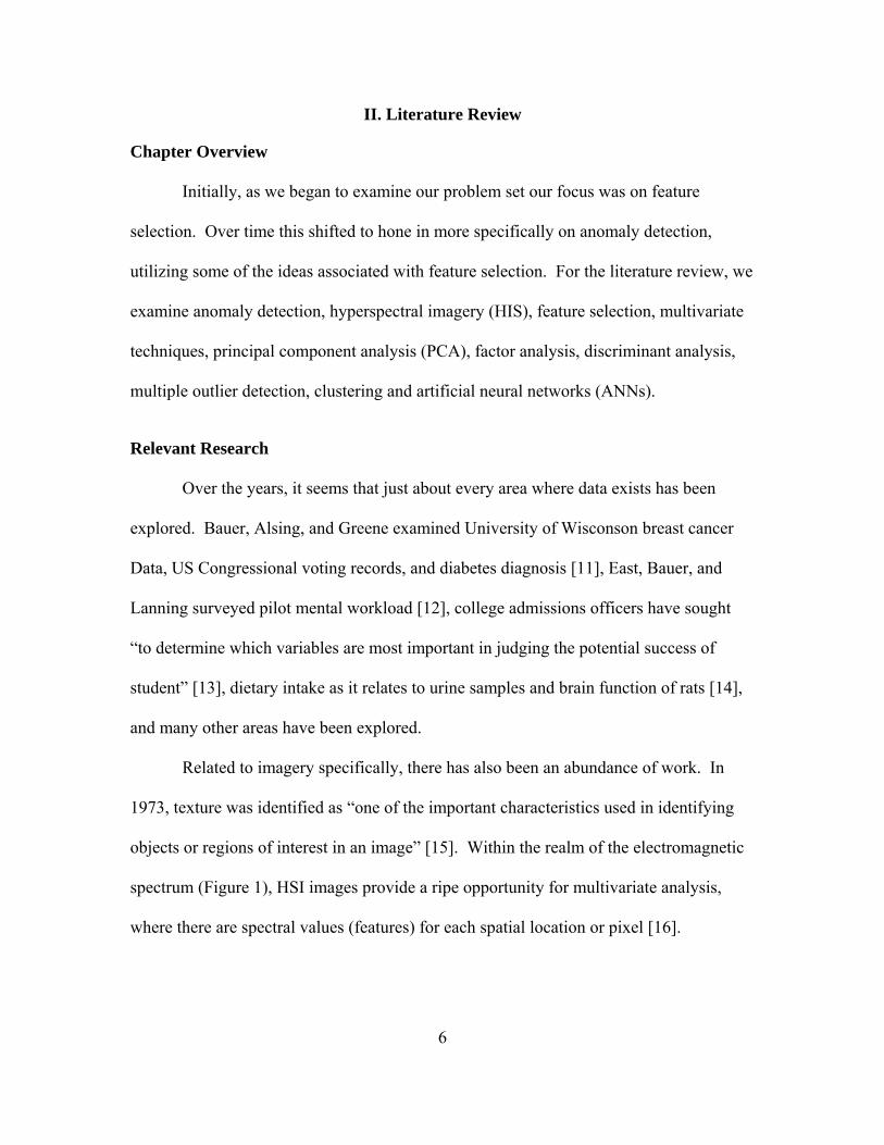
Related to imagery specifically, there has also been an abundance of work. In
1973, texture was identified as “one of the important characteristics used in identifying
objects or regions of interest in an image” [15]. Within the realm of the electromagnetic
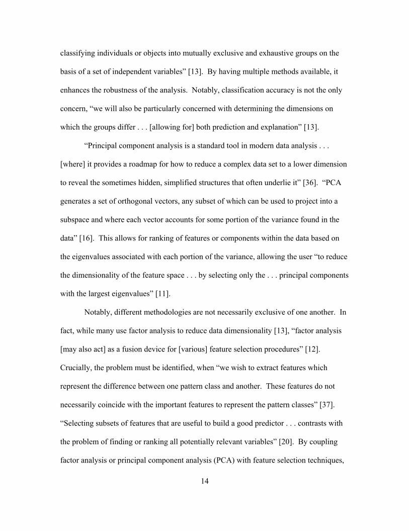
spectrum (Figure 1), HSI images provide a ripe opportunity for multivariate analysis,
where there are spectral values (features) for each spatial location or pixel [16].
7
Figure 1: The Electromagnetic Spectrum [17]
Given that magnitude of possible applications and some of the difficulties
associated research has abounded. Smetek worked at “hyperspectral target detection by
developing autonomous anomaly detection and signature matching methodologies that
reduce false alarms relative to existing benchmark detectors” [18]. Essentially, he
“adapts multivariate outlier detection algorithms for use with hyperspectral datasets
containing tens of thousands of non-homogeneous, high-dimensional spectral signatures”
[18]. Johnson “[employed] independent component analysis (ICA) to unmix HSI images.
Via new techniques to fully automate feature extraction, feature selection, and target
pixel identification” [19]. This was extended “for global anomaly detection on a variety
of HSI, utilizing fusion of spatial and spectral information, factor analysis, clustering, and
screening” [16].
8
Feature Selection
For decades, feature selection has been a critical component of synthesizing,
interacting with, and analyzing vast amounts of data. Truly, “variable and feature
selection have become the focus of much research in areas of application for which
datasets with tens or hundreds of thousands of variables are available” [20]. In fact, “the
remarkable development of computing power and other technology has allowed scientists
to collect data of unprecedented size and complexity” [21]. Moreover, while it is
certainly applied to datasets with tens or hundreds of thousands or even millions of
variables, feature selection has been applied to datasets of much lower dimensionality as
well [16]. “Feature selection may be employed to improve a classification model . . . by
eliminating non-informative features . . . [and it] may also be used to gain further insight
into the rationale underlying class divisions within a particular domain” [14].
Simultaneously, in feature selection the desire is to minimize the computational time to
the greatest degree possible, recognizing that in some cases reduced time is the preferred
objective as long as adequate accuracy is maintained [12]. Feature selection enhances the
probability of ascertaining insight into varying situations, while minimizing the Type I
and Type II errors associated with the predicted results of those situations. It is important
to remember that as selecting the appropriate features will enhance the predictive nature
of the models examined, but it is crucial to ensure that we are making selections based on
the appropriate response. We have to determine the right question or questions; what is
the crucial result or response and why. And we certainly do not want the “right answer
for the wrong question” [22].
9
Anomaly Detection
This leads us to field of anomaly detection. “Anomaly detection refers to the
problem of finding patterns in data that do not conform to expected behavior . . . often
referred to as anomalies, outliers, discordant observations, exceptions, aberrations,
surprises, peculiarities, or contaminants” [23]. The “goal is to discover the true outliers
and avoid mistakenly marking normal points as abnormal. In other words, a good
anomaly detector must have a high detection rate and low false alarm rate” [24]. And
even a low false alarm rate does not necessarily provide all the information of importance
regarding the anomaly detected, leading to anomaly classification. Which is
“implemented in a three-stage process, first by anomaly detection to find potential
targets, followed by target discrimination to cluster the detected anomalies into separate
target classes, and concluded by a classifier to achieve target classification” [5].
Classifying anomalies holds importance, because it is not just important to find the
anomalies, “it is often more important to make sure that those anomalies that are reported
to the user are in fact interesting” [25]. Notably, “experiments show that anomaly
classification performs very differently from anomaly detection” [5]. Consistent with
[26], [27], Chandola et al. reminds us that “anomaly detection is related to, but distinct
from noise removal and noise accommodation . . . [where] noise can be defined as a
phenomenon in data that is not of interest to the analyst, but acts as a hinderance to data
analsyis” [23] .
Dimensionality
Numerous methodologies have been applied to increase the quality of feature
selection. Importantly, feature selection is not limited to one field, but has been a chief
10
concern in numerous industries, fields, and problem sets [11], [13], [16]. In applying
feature selection methodologies, one recognizes that often times the use of all available
data to establish the model can “[result] in poor classification accuracy due to the
distracting effect of numerous redundant and/or unnecessary variables” [12].
Additionally, we know that, from using ANNs, “as the number of features grows, the
number of training vectors required grows exponentially”, obviously having potentially
deleterious effects on computational time [11]. Screening to reduce these redundancies
adds robustness and prediction accuracy to our solution space. However, one of the great
things about feature selection is that it helps provide a framework to determine which
variables should stay in the model. There are even cases where “noise reduction and
consequently better class separation may be obtained by adding variables that are
presumably redundant”, and this seems to be especially true, when utilizing methods
more commonly associated with ranking instead of prediction [20].
In the case of HSI, an understanding of dimensionality is truly critical because
there are specific hyperspectral bands that tend to absorb the incident energy associated
with natural materials [16]. By identifying these atmospheric absorption bands, one
reduces the dimensionality of an image, by removing those bands in which the sensor
detects random noise [18].
Screening Methods and Saliency Measures
Since a primary component to the validity of feature selection within a scenario is
this ability to maintain the features which discriminate between classes, screening
methodologies are a crucial component in the success of feature selection. Various
methods have been proposed utilizing saliency measures. While “a number of feature
11
saliency measures can be used to evaluate and rank the relative importance of candidate
features . . . a saliency measure alone does not indicate how many of the candidate
features should be used,” once again returning to the importance of asking the right
question [28]. The Belue-Bauer screening method utilizes “a confidence interval
constructed around [the average saliency of injected noise allowing] for the identification
of features that contribute little to classification” [29]. Demonstrably, the utilization of
“an appropriate hypothesis test to account for naturally paired observations of feature
saliency measures and the use of a Bonferroni-type test statistic to reflect a conservative
degree of statistical confidence for joint hypothesis testing. . . indicates that the truly
noisy features can be consistently identified” [28]. Still other methods “measure the
relative size of the weight vector emanating from each feature” [30]. Additional evidence
indicates that while various screening methods “typically require between 10 and 30
training runs” the use of signal-to-noise (SNR) saliency measures may only require one
training run potentially resulting in a significant reduction of computational processing
time [11]. Other saliency measures have “[evaluated] each feature with respect to
relative changes in either the neural network’s output or the neural network’s probability
of error” [30].
Techniques
ANNs have long been a technique tied to feature selection, recognizing, as
previously indicated that, “the relevance of a given input feature in a neural network is
important in classification and prediction problems. “ANNs are desirable because they
provide a well-structured framework to discover non-linear relationships within data sets
that are considered ‘noisy’ or complex” [31]. In fact quite often, one is faced with a large
12
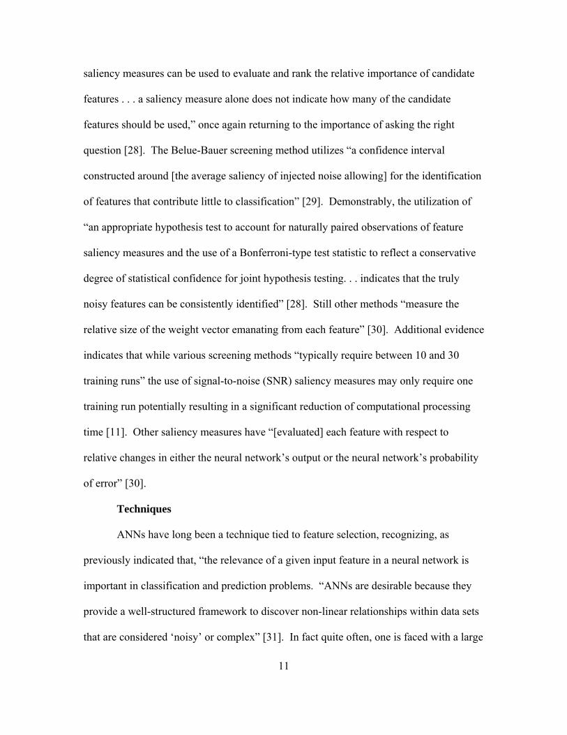
number of candidate features which may or may not be useful for the problem at hand”
[28]. Figure 2 shows the framework of the neural network.
Figure 2: Neural Network Structure (Copied from Belue & Bauer, 1995)
Essentially, ANNs “are networks or systems formed out of many highly
interconnected nonlinear memoryless computing elements or subsystems . . . [that] can be
represented mathematically as a weighted, directed graph” [32]. “There is also an
appealing quality to [their] ‘brain-like’structure” [29]. In fact it has been recognized that:
Computational properties of use to biological organisms or to the construction of
computers can emerge as collective properties of systems having a large number
13
of simple equivalent components (or neurons). . . . The collective properties of
this model produce a content addressable memory which correctly yields an entire
memory from any subpart of sufficient size [33].
“Intuitively an analyst would like to include only those features that make a significant
contribution to the network”, and given the networks structure as features are extracted
and noise is removed and reduced the addressable memory can actually yield greater
predictability [29]. Three processes take place to maximize the predictability of the
ANN, first the network is trained with some sample of data, then it is internally validated
with another, typically smaller sample, before it is finally tested for classification
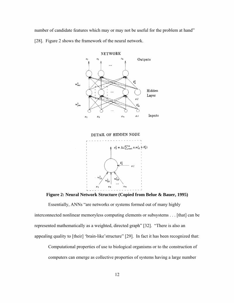
accuracy on the remainder of the data [11]. With autoencoding in particular, the goal is
for the ANN to learn “the underlying feature structure of the data” that makes the data
distinctive, then that ANN can be used for determining the classification of other data
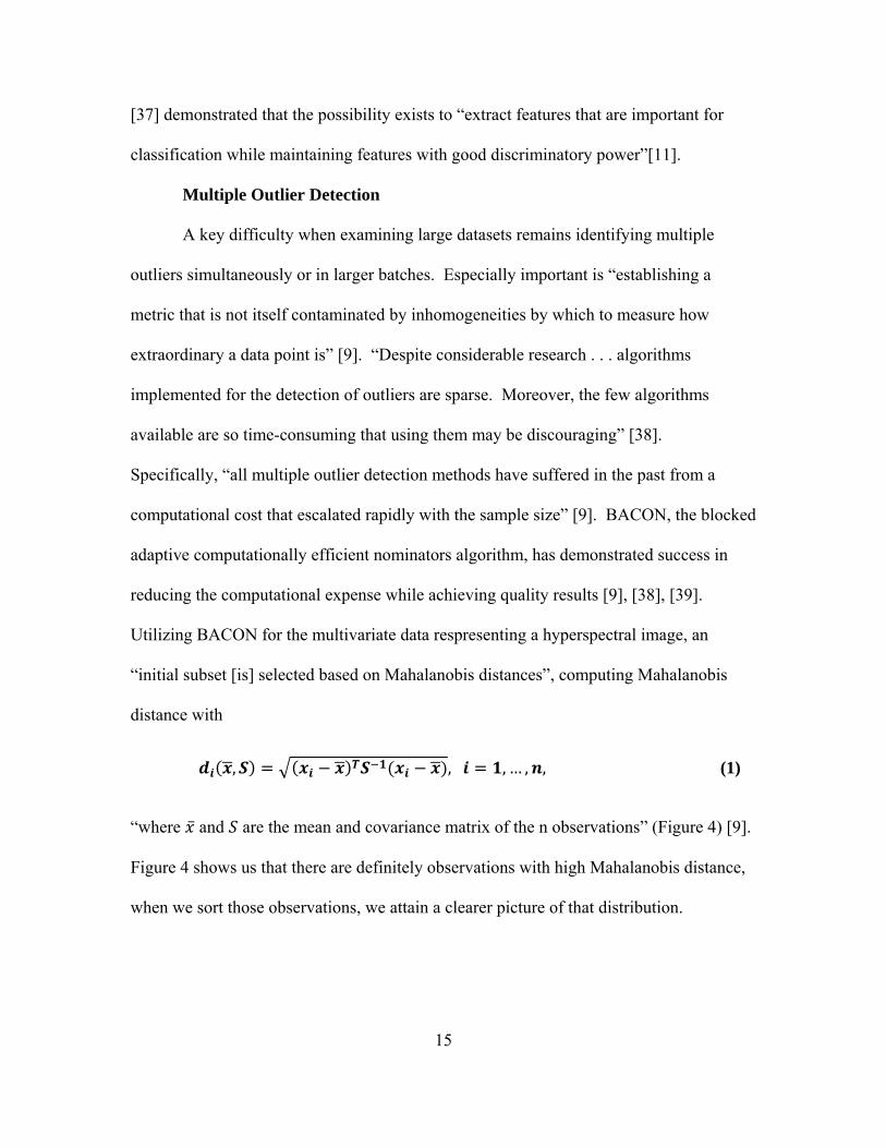
[34]. Figure 3 shows how the input layer and output layer are the same size, with the
goal of finding the weights between nodes that yield the minimum reconstructive error
between the input and the output.
Figure 3: Autoencoder Structure [35]
Similar to ANNs, discriminant analysis trains on one set of data to be predictive
for another sample of data. “Discriminant analysis is a statistical technique for
14
classifying individuals or objects into mutually exclusive and exhaustive groups on the
basis of a set of independent variables” [13]. By having multiple methods available, it
enhances the robustness of the analysis. Notably, classification accuracy is not the only
concern, “we will also be particularly concerned with determining the dimensions on
which the groups differ . . . [allowing for] both prediction and explanation” [13].
“Principal component analysis is a standard tool in modern data analysis . . .
[where] it provides a roadmap for how to reduce a complex data set to a lower dimension
to reveal the sometimes hidden, simplified structures that often underlie it” [36]. “PCA
generates a set of orthogonal vectors, any subset of which can be used to project into a
subspace and where each vector accounts for some portion of the variance found in the
data” [16]. This allows for ranking of features or components within the data based on
the eigenvalues associated with each portion of the variance, allowing the user “to reduce
the dimensionality of the feature space . . . by selecting only the . . . principal components
with the largest eigenvalues” [11].
Notably, different methodologies are not necessarily exclusive of one another. In
fact, while many use factor analysis to reduce data dimensionality [13], “factor analysis
[may also act] as a fusion device for [various] feature selection procedures” [12].
Crucially, the problem must be identified, when “we wish to extract features which
represent the difference between one pattern class and another. These features do not
necessarily coincide with the important features to represent the pattern classes” [37].
“Selecting subsets of features that are useful to build a good predictor . . . contrasts with
the problem of finding or ranking all potentially relevant variables” [20]. By coupling
factor analysis or principal component analysis (PCA) with feature selection techniques,
15
[37] demonstrated that the possibility exists to “extract features that are important for
classification while maintaining features with good discriminatory power”[11].
Multiple Outlier Detection
A key difficulty when examining large datasets remains identifying multiple
outliers simultaneously or in larger batches. Especially important is “establishing a
metric that is not itself contaminated by inhomogeneities by which to measure how
extraordinary a data point is” [9]. “Despite considerable research . . . algorithms
implemented for the detection of outliers are sparse. Moreover, the few algorithms
available are so time-consuming that using them may be discouraging” [38].
Specifically, “all multiple outlier detection methods have suffered in the past from a
computational cost that escalated rapidly with the sample size” [9]. BACON, the blocked
adaptive computationally efficient nominators algorithm, has demonstrated success in
reducing the computational expense while achieving quality results [9], [38], [39].
Utilizing BACON for the multivariate data respresenting a hyperspectral image, an
“initial subset [is] selected based on Mahalanobis distances”, computing Mahalanobis
distance with
, , , … , , (1)
“where ̅ and are the mean and covariance matrix of the n observations” (Figure 4) [9].
Figure 4 shows us that there are definitely observations with high Mahalanobis distance,
when we sort those observations, we attain a clearer picture of that distribution.
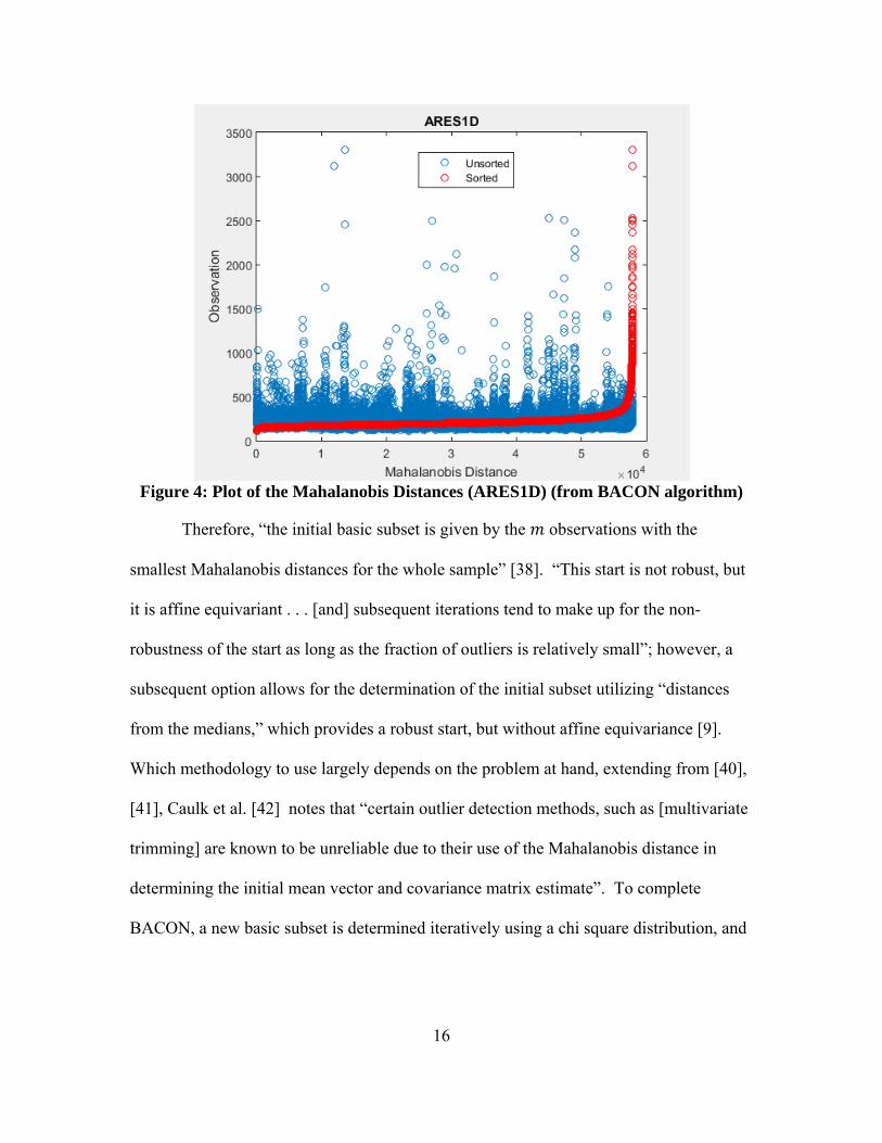
16
Figure 4: Plot of the Mahalanobis Distances (ARES1D) (from BACON algorithm)
Therefore, “the initial basic subset is given by the observations with the
smallest Mahalanobis distances for the whole sample” [38]. “This start is not robust, but
it is affine equivariant . . . [and] subsequent iterations tend to make up for the non-
robustness of the start as long as the fraction of outliers is relatively small”; however, a
subsequent option allows for the determination of the initial subset utilizing “distances
from the medians,” which provides a robust start, but without affine equivariance [9].
Which methodology to use largely depends on the problem at hand, extending from [40],
[41], Caulk et al. [42] notes that “certain outlier detection methods, such as [multivariate
trimming] are known to be unreliable due to their use of the Mahalanobis distance in
determining the initial mean vector and covariance matrix estimate”. To complete
BACON, a new basic subset is determined iteratively using a chi square distribution, and
17
the algorithm continues “until the size of the basic subset no longer changes, [whereby
we] nominate the observations excluded by the final basic subset as outliers” [9].
The Reed-Xiaoli (RX) algorithm is another algorithm that has the potential to
partition data, it “was developed from the generalized likelihood ratio (GLR) test . . .
based on the suggestion that most optical image clutter can be modeled as a Gaussian
random process with possibly a rapidly fluctuating space-varying mean and a more
slowly varying covariance” [43]. As shown by [44], [45], RX “is considered as a
benchmark” detector for comparison due to its simplicity” [46].
Clustering
“Clustering is usually considered to be the problem of partitioning a single set of
unlabeled points . . . [where] one of the most common iterative, [non-hierarchical]
algorithms is the K-means algorithm, broadly used for its simplicity of implementation
and convergence speed” [40]. “The k-means process was originally devised in an attempt
to find a feasible method of computing such an optimal partition” [47], where it
“produces relatively high quality clusters considering the low level of computation
required” [40]. K-means
“requires that the number of clusters used to classify the dataset will be pre-
determined. It is based on determining arbitrary centers for the desired clusters,
associating the samples with the clusters by using a pre-determined distance
measurement, iteratively changing the center of the clusters and then re-
associating the samples” [48].
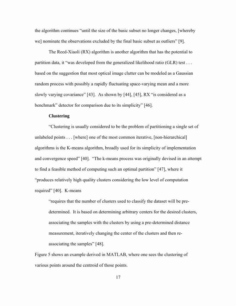
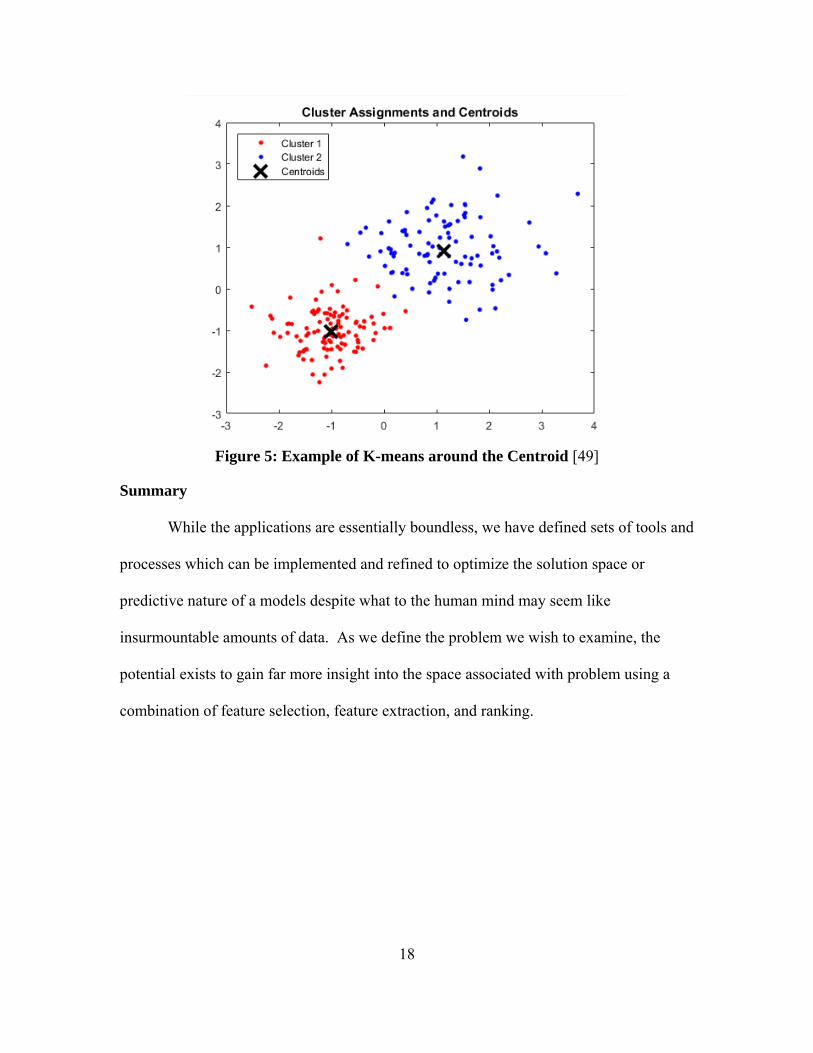
Figure 5 shows an example derived in MATLAB, where one sees the clustering of
various points around the centroid of those points.
18
Figure 5: Example of K-means around the Centroid [49]
Summary
While the applications are essentially boundless, we have defined sets of tools and
processes which can be implemented and refined to optimize the solution space or
predictive nature of a models despite what to the human mind may seem like
insurmountable amounts of data. As we define the problem we wish to examine, the
potential exists to gain far more insight into the space associated with problem using a
combination of feature selection, feature extraction, and ranking.
19
III. Methodology
Chapter Overview
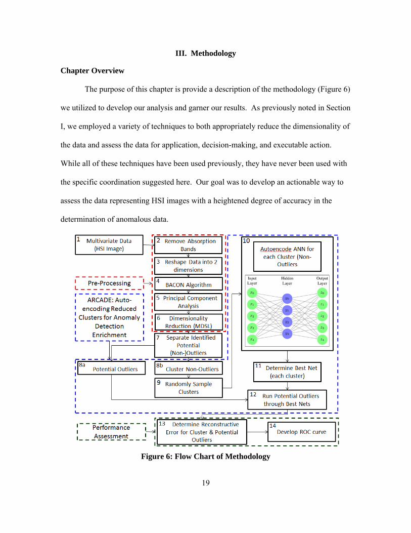
The purpose of this chapter is provide a description of the methodology (Figure 6)
we utilized to develop our analysis and garner our results. As previously noted in Section
I, we employed a variety of techniques to both appropriately reduce the dimensionality of
the data and assess the data for application, decision-making, and executable action.
While all of these techniques have been used previously, they have never been used with
the specific coordination suggested here. Our goal was to develop an actionable way to
assess the data representing HSI images with a heightened degree of accuracy in the
determination of anomalous data.
Figure 6: Flow Chart of Methodology

20
Test Subjects
In order to test and develop our methodology, we utilized a set of test images
maintained by the Air Force Institute of Technology’s (AFIT’s) Sensor Fusion
Laboratory derived from the HYDICE sensor. This provided us the opportunity to test
our methodology against truth data already available for the images tested. Our testing
was initially conducted against the image ARES1F, prior to expanding to ARES1D and
ARES2D.
Summary
As stated previously, we utilized various methods in combination and
coordination to assess and analyze potential anomalies within HSI images. We will
discuss the method in association with the numbered steps indicated in the upper left
hand corners of the Flow Chart of Methodology (Figure 6).
Step 1 – Multivariate Data
We select the image for testing. In this case, HYDICE sensor images as discussed
above beginning with image ARES1F prior to assessing both ARES1D and ARES2D.
Pre-Processing
Step 2 – Remove Absorption Bands
As discussed in Section II, we acknowledge that HSI images contain absorption
bands that generate noise within the images; therefore, we reduced dimensionality using
the pre-determined absorption bands. This reduces the dimensionality of the image from
210 dimensions (Hyperspectral Bands) to 145 [50].
21
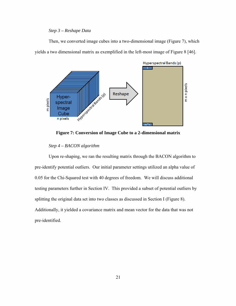
Step 3 – Reshape Data
Then, we converted image cubes into a two-dimensional image (Figure 7), which
yields a two dimensional matrix as exemplified in the left-most image of Figure 8 [46].
Figure 7: Conversion of Image Cube to a 2-dimensional matrix
Step 4 – BACON algorithm
Upon re-shaping, we ran the resulting matrix through the BACON algorithm to
pre-identify potential outliers. Our initial parameter settings utilized an alpha value of
0.05 for the Chi-Squared test with 40 degrees of freedom. We will discuss additional
testing parameters further in Section IV. This provided a subset of potential outliers by
splitting the original data set into two classes as discussed in Section I (Figure 8).
Additionally, it yielded a covariance matrix and mean vector for the data that was not
pre-identified.
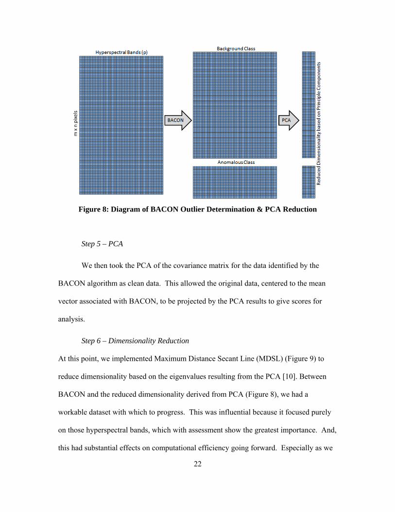
22
Figure 8: Diagram of BACON Outlier Determination & PCA Reduction
Step 5 – PCA
We then took the PCA of the covariance matrix for the data identified by the
BACON algorithm as clean data. This allowed the original data, centered to the mean
vector associated with BACON, to be projected by the PCA results to give scores for
analysis.
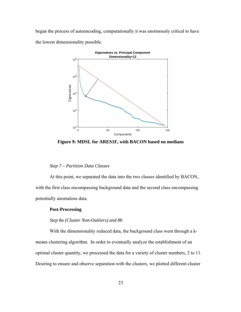
Step 6 – Dimensionality Reduction
At this point, we implemented Maximum Distance Secant Line (MDSL) (Figure 9) to
reduce dimensionality based on the eigenvalues resulting from the PCA [10]. Between
BACON and the reduced dimensionality derived from PCA (Figure 8), we had a
workable dataset with which to progress. This was influential because it focused purely
on those hyperspectral bands, which with assessment show the greatest importance. And,
this had substantial effects on computational efficiency going forward. Especially as we
23
began the process of autoencoding, computationally it was enormously critical to have
the lowest dimensionality possible.
Figure 9: MDSL for ARES1F, with BACON based on medians
Step 7 – Partition Data Classes
At this point, we separated the data into the two classes identified by BACON,
with the first class encompassing background data and the second class encompassing
potentially anomalous data.
Post-Processing
Step 8a (Cluster Non-Outliers) and 8b
With the dimensionality reduced data, the background class went through a k-
means clustering algorithm. In order to eventually analyze the establishment of an
optimal cluster quantity, we processed the data for a variety of cluster numbers, 2 to 11.
Desiring to ensure and observe separation with the clusters, we plotted different cluster
Components0 50 100 150
100
102
104
106
108
Eigenvalues vs. Principal ComponentDimensionality=12
24
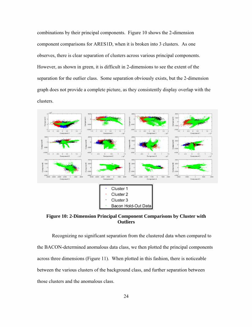
combinations by their principal components. Figure 10 shows the 2-dimension
component comparisons for ARES1D, when it is broken into 3 clusters. As one
observes, there is clear separation of clusters across various principal components.
However, as shown in green, it is difficult in 2-dimensions to see the extent of the
separation for the outlier class. Some separation obviously exists, but the 2-dimension
graph does not provide a complete picture, as they consistently display overlap with the
clusters.
Figure 10: 2-Dimension Principal Component Comparisons by Cluster with
Outliers
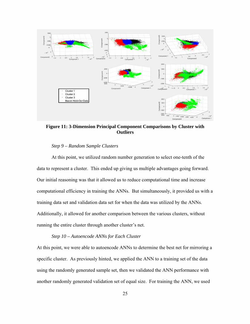
Recognizing no significant separation from the clustered data when compared to
the BACON-determined anomalous data class, we then plotted the principal components
across three dimensions (Figure 11). When plotted in this fashion, there is noticeable
between the various clusters of the background class, and further separation between
those clusters and the anomalous class.
25
Figure 11: 3-Dimension Principal Component Comparisons by Cluster with
Outliers
Step 9 – Random Sample Clusters
At this point, we utilized random number generation to select one-tenth of the
data to represent a cluster. This ended up giving us multiple advantages going forward.
Our initial reasoning was that it allowed us to reduce computational time and increase
computational efficiency in training the ANNs. But simultaneously, it provided us with a
training data set and validation data set for when the data was utilized by the ANNs.
Additionally, it allowed for another comparison between the various clusters, without
running the entire cluster through another cluster’s net.
Step 10 – Autoencode ANNs for Each Cluster
At this point, we were able to autoencode ANNs to determine the best net for mirroring a
specific cluster. As previously hinted, we applied the ANN to a training set of the data
using the randomly generated sample set, then we validated the ANN performance with
another randomly generated validation set of equal size. For training the ANN, we used
26
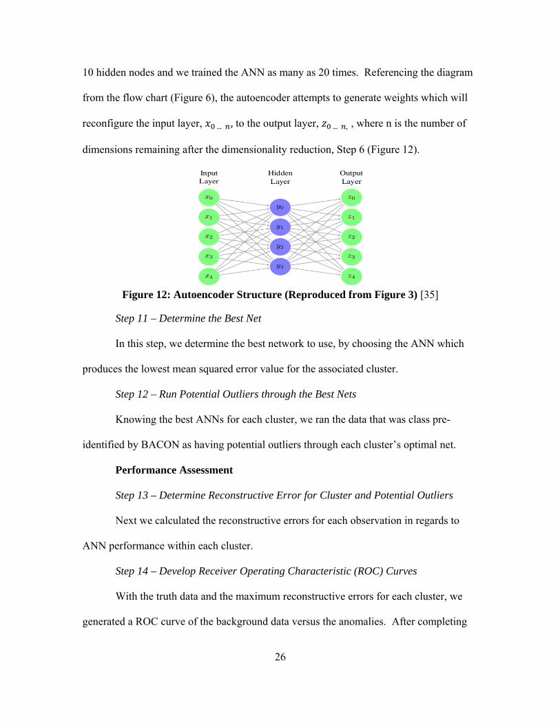
10 hidden nodes and we trained the ANN as many as 20 times. Referencing the diagram
from the flow chart (Figure 6), the autoencoder attempts to generate weights which will
reconfigure the input layer, ... , to the output layer, ... , , where n is the number of
dimensions remaining after the dimensionality reduction, Step 6 (Figure 12).
Figure 12: Autoencoder Structure (Reproduced from Figure 3) [35]
Step 11 – Determine the Best Net
In this step, we determine the best network to use, by choosing the ANN which
produces the lowest mean squared error value for the associated cluster.
Step 12 – Run Potential Outliers through the Best Nets
Knowing the best ANNs for each cluster, we ran the data that was class pre-
identified by BACON as having potential outliers through each cluster’s optimal net.
Performance Assessment
Step 13 – Determine Reconstructive Error for Cluster and Potential Outliers
Next we calculated the reconstructive errors for each observation in regards to
ANN performance within each cluster.
Step 14 – Develop Receiver Operating Characteristic (ROC) Curves
With the truth data and the maximum reconstructive errors for each cluster, we
generated a ROC curve of the background data versus the anomalies. After completing

27
this for various images, we were able to determine a threshold which we were
comfortable and classify the observations within the originally designated anomalous
class as true anomalies or as background.
28
IV. Analysis and Results
Chapter Overview
We specifically examined three hyperspectral imagery (HSI) images in an effort
to validate the algorithmic and methodological results as compared to the known
anomalies within the specified images. Since the Autoencoded Reduced Clustering for
Anomaly Dectection Enrichment (ARCADE) parameters are modifiable, we could
examine the each of the images using our base methodology independently. In
conducting the analysis, we developed receiver operating characteristic (ROC) curves to
measure our method’s anomaly prediction accuracy. Furthermore, we examine various
parameter settings throughout the process to gain insight into how those parameters affect
the overall methodology.
In addition to comparing the results between the images themselves, we also
compared the results of the methodological variations for each image. This provided
some insight into inelasticity of various parameters and the robustness of the ARCADE
method. While our base methodology (Figure 6) was described in Section III, this
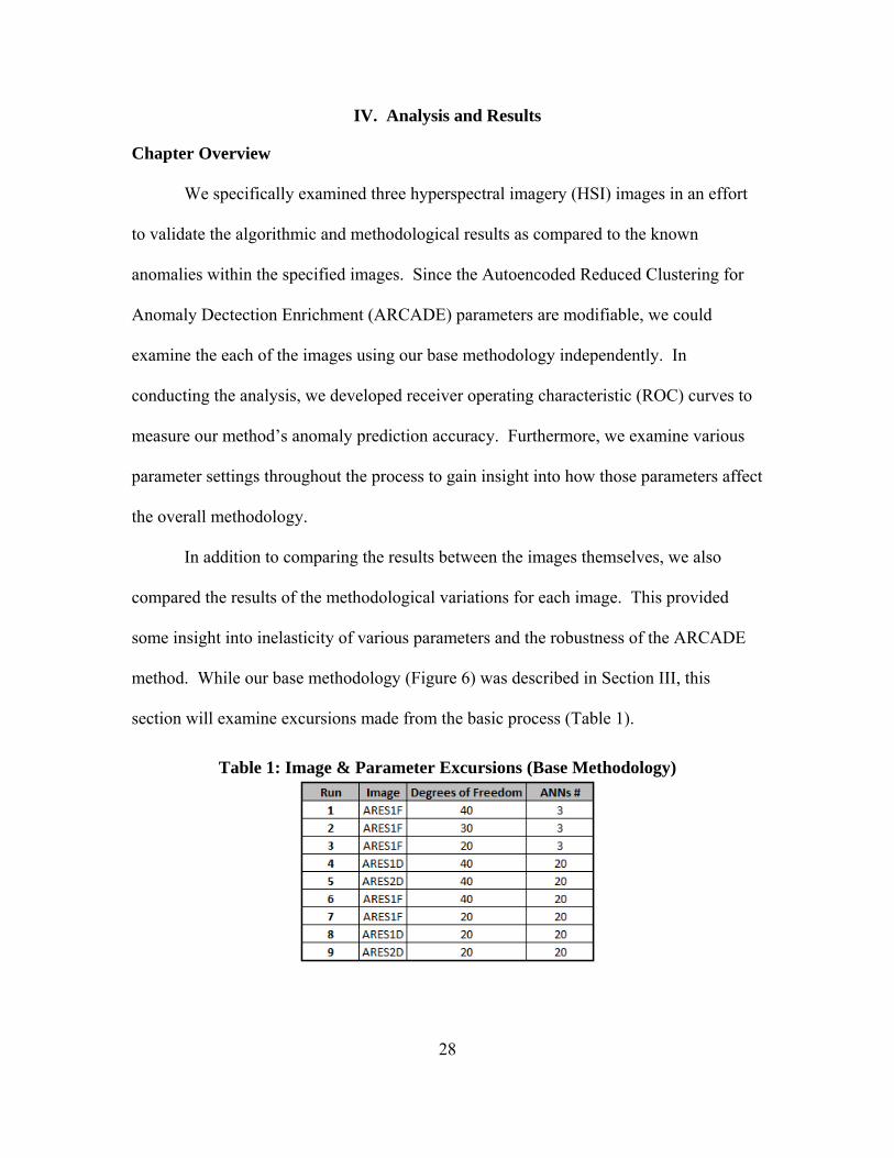
section will examine excursions made from the basic process (Table 1).
Table 1: Image & Parameter Excursions (Base Methodology)
29
We initially examined the basic methodology (Figure 6), considering various
parameter changes, while recognizing the possibility of using different pre-processing
techniques. Table 1 shows the parameter changes that were explored in examining our
basic methodology. Following a description of the results associated with the base
methodology and the parameter excursions associated with the base methodology, we
will describe five variations that were made regarding our pre-processing techniques.
These variations and excursions provide substantial information to inform the quality of
our results and conclusions. In our initial excursions from our base methodology, we
examined the number of degrees of freedom associated with the BACON algorithm and
we examined the number of ANNs. For degrees of freedom, we ranged from 20 to 40,
and for ANNs, we ranged from 3 to 20 to determine if additional processing would
impact the results.
Results of Base Methodology
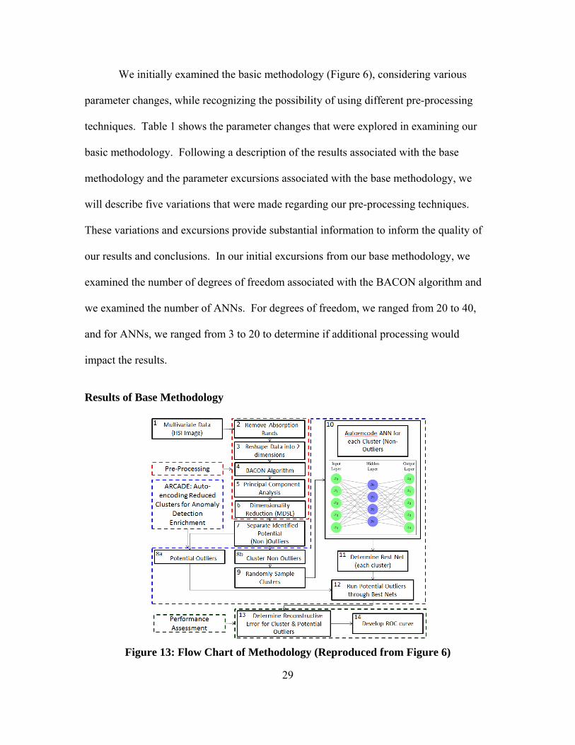
Figure 13: Flow Chart of Methodology (Reproduced from Figure 6)
30
Step 1 to 3 – Image Processing
After importing the images, we removed the absorption bands, and re-
dimensionalized the data into two dimensions as previously described.
Step 4 – BACON algorithm
As discussed in Sections II and III, BACON finds a pre-identified selection of
potential outlier points, which we define as our anomalous class, while considering all
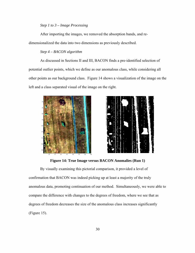
other points as our background class. Figure 14 shows a visualization of the image on the
left and a class separated visual of the image on the right.
Figure 14: True Image versus BACON Anomalies (Run 1)
By visually examining this pictorial comparison, it provided a level of
confirmation that BACON was indeed picking up at least a majority of the truly
anomalous data, promoting continuation of our method. Simultaneously, we were able to
compare the difference with changes to the degrees of freedom, where we see that as
degrees of freedom decreases the size of the anomalous class increases significantly
(Figure 15).
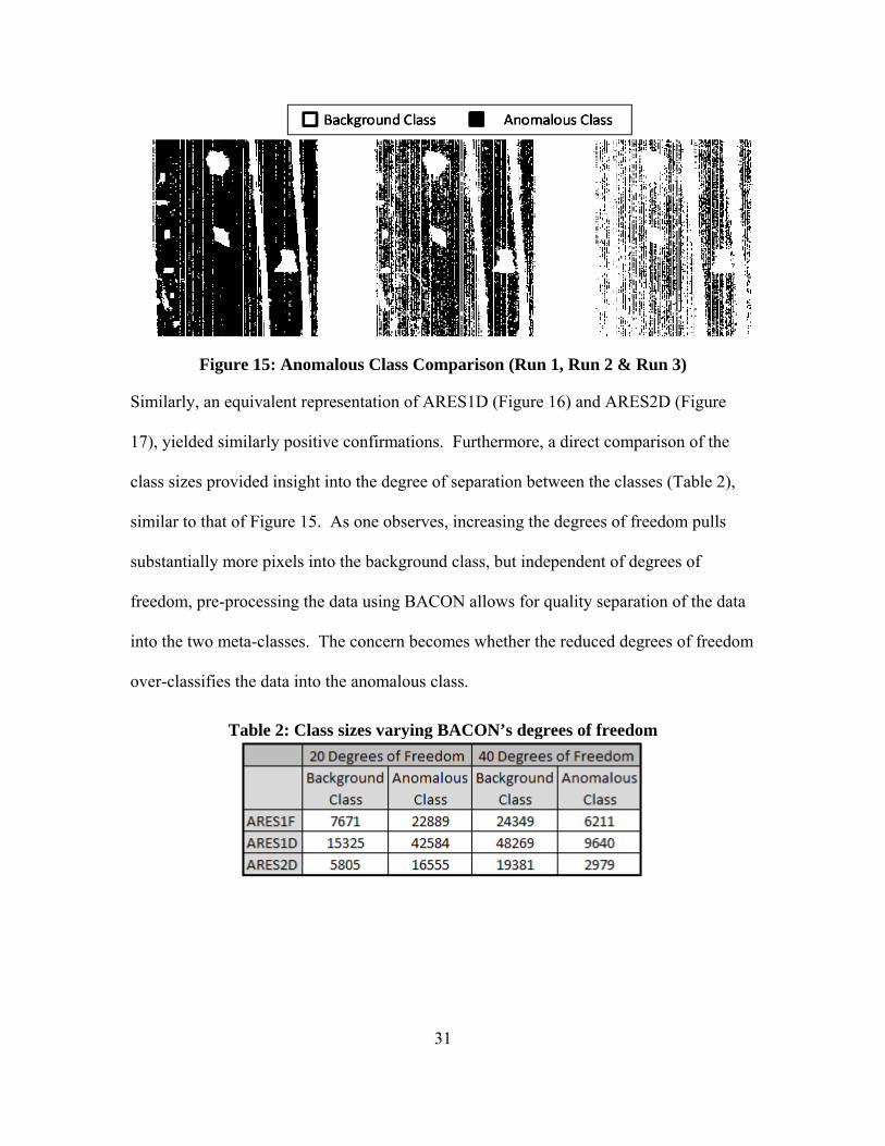
31
Figure 15: Anomalous Class Comparison (Run 1, Run 2 & Run 3)
Similarly, an equivalent representation of ARES1D (Figure 16) and ARES2D (Figure
17), yielded similarly positive confirmations. Furthermore, a direct comparison of the
class sizes provided insight into the degree of separation between the classes (Table 2),
similar to that of Figure 15. As one observes, increasing the degrees of freedom pulls
substantially more pixels into the background class, but independent of degrees of
freedom, pre-processing the data using BACON allows for quality separation of the data
into the two meta-classes. The concern becomes whether the reduced degrees of freedom
over-classifies the data into the anomalous class.
Table 2: Class sizes varying BACON’s degrees of freedom
32
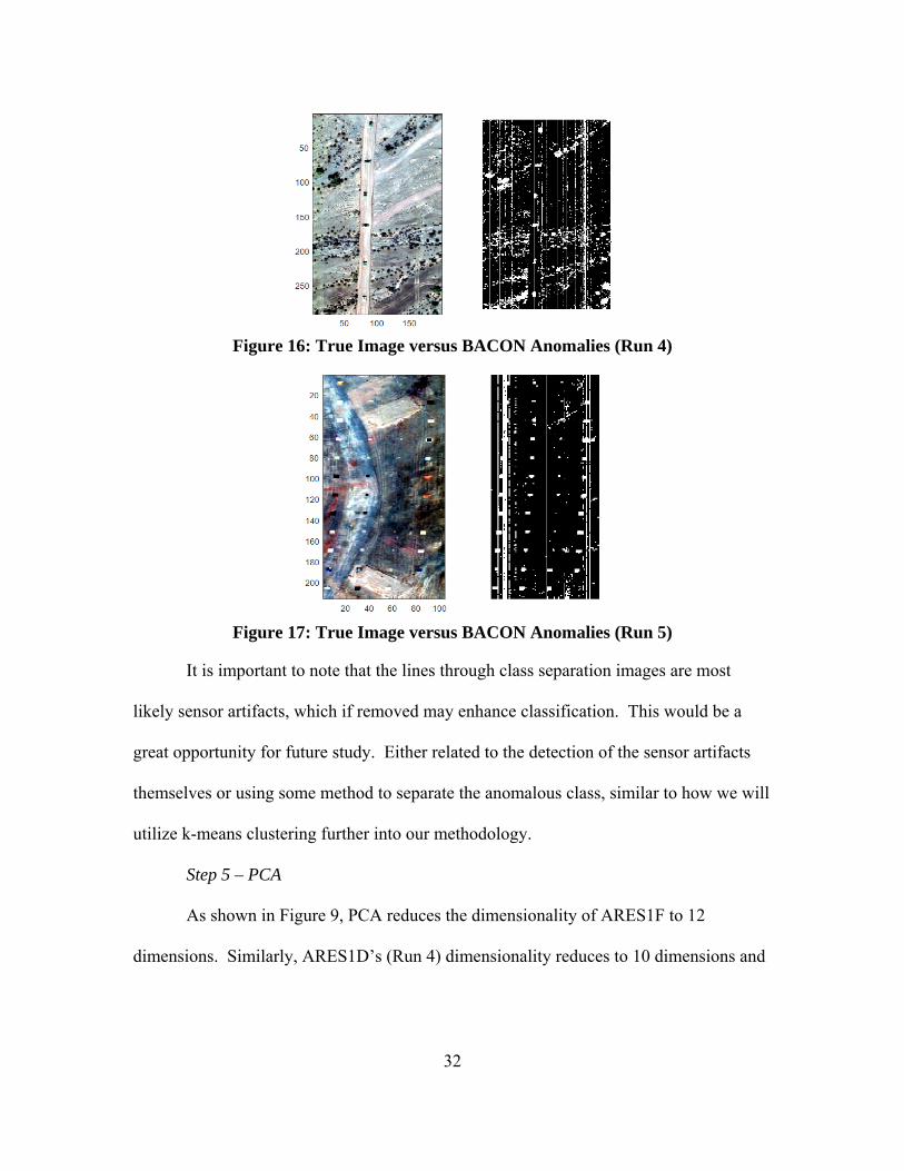
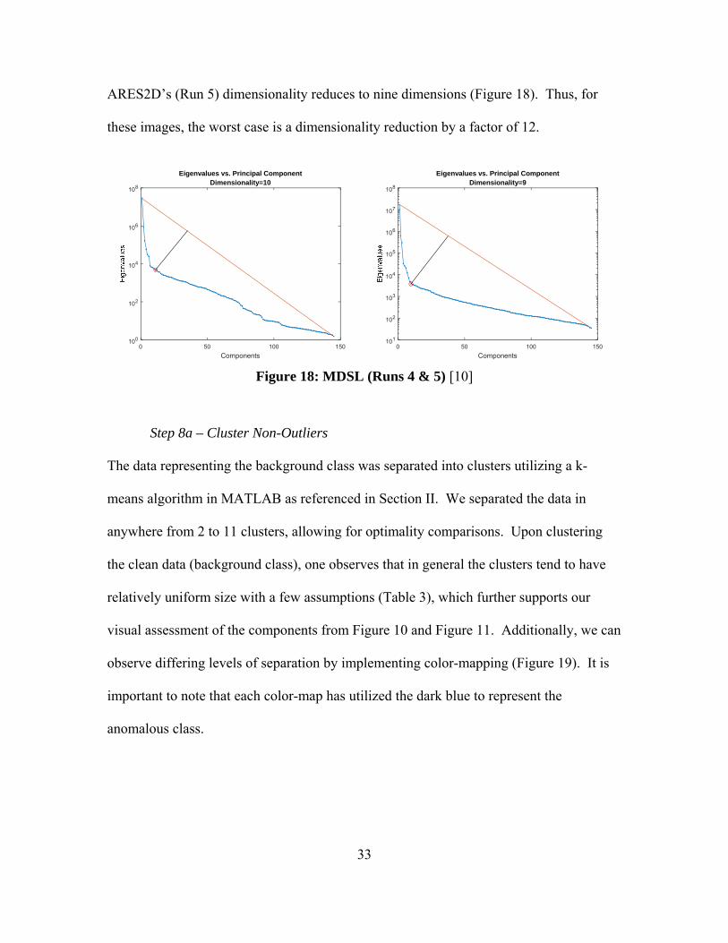
Figure 16: True Image versus BACON Anomalies (Run 4)
Figure 17: True Image versus BACON Anomalies (Run 5)
It is important to note that the lines through class separation images are most
likely sensor artifacts, which if removed may enhance classification. This would be a
great opportunity for future study. Either related to the detection of the sensor artifacts
themselves or using some method to separate the anomalous class, similar to how we will
utilize k-means clustering further into our methodology.
Step 5 – PCA
As shown in Figure 9, PCA reduces the dimensionality of ARES1F to 12
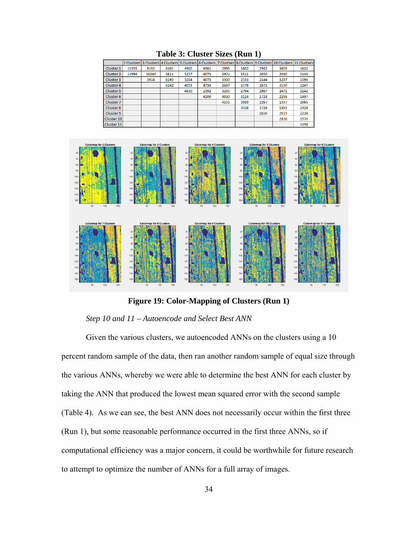
dimensions. Similarly, ARES1D’s (Run 4) dimensionality reduces to 10 dimensions and
33
ARES2D’s (Run 5) dimensionality reduces to nine dimensions (Figure 18). Thus, for
these images, the worst case is a dimensionality reduction by a factor of 12.
Figure 18: MDSL (Runs 4 & 5) [10]
Step 8a – Cluster Non-Outliers
The data representing the background class was separated into clusters utilizing a k-
means algorithm in MATLAB as referenced in Section II. We separated the data in
anywhere from 2 to 11 clusters, allowing for optimality comparisons. Upon clustering
the clean data (background class), one observes that in general the clusters tend to have
relatively uniform size with a few assumptions (Table 3), which further supports our
visual assessment of the components from Figure 10 and Figure 11. Additionally, we can
observe differing levels of separation by implementing color-mapping (Figure 19). It is
important to note that each color-map has utilized the dark blue to represent the
anomalous class.
Components0 50 100 150
100
102
104
106
108
Eigenvalues vs. Principal ComponentDimensionality=10
Components0 50 100 150
101
102
103
104
105
106
107
108
Eigenvalues vs. Principal ComponentDimensionality=9
34
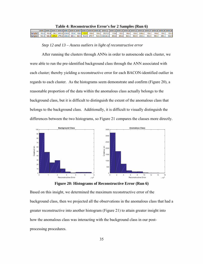
Table 3: Cluster Sizes (Run 1)
Figure 19: Color-Mapping of Clusters (Run 1)
Step 10 and 11 – Autoencode and Select Best ANN
Given the various clusters, we autoencoded ANNs on the clusters using a 10
percent random sample of the data, then ran another random sample of equal size through
the various ANNs, whereby we were able to determine the best ANN for each cluster by
taking the ANN that produced the lowest mean squared error with the second sample
(Table 4). As we can see, the best ANN does not necessarily occur within the first three
(Run 1), but some reasonable performance occurred in the first three ANNs, so if
computational efficiency was a major concern, it could be worthwhile for future research
to attempt to optimize the number of ANNs for a full array of images.
35
Table 4: Reconstructive Error's for 2 Samples (Run 6)
Step 12 and 13 – Assess outliers in light of reconstructive error
After running the clusters through ANNs in order to autoencode each cluster, we
were able to run the pre-identified background class through the ANN associated with
each cluster; thereby yielding a reconstructive error for each BACON-identified outlier in
regards to each cluster. As the histograms seem demonstrate and confirm (Figure 20), a
reasonable proportion of the data within the anomalous class actually belongs to the
background class, but it is difficult to distinguish the extent of the anomalous class that
belongs to the background class. Additionally, it is difficult to visually distinguish the
differences between the two histograms, so Figure 21 compares the classes more directly.
Figure 20: Histograms of Reconstructive Error (Run 6)
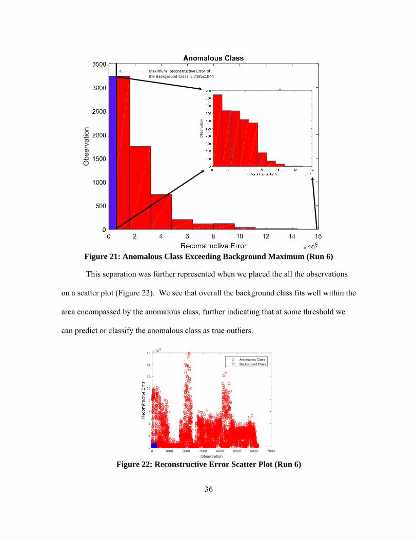
Based on this insight, we determined the maximum reconstructive error of the
background class, then we projected all the observations in the anomalous class that had a
greater reconstructive into another histogram (Figure 21) to attain greater insight into
how the anomalous class was interacting with the background class in our post-
processing procedures.
Reconstructive Error 1040 1 2 3 4 5 6
0
10
20
30
40
50
60
70
80
90
100Background Class
Reconstructive Error 1050 2 4 6 8 10 12 14 16
0
500
1000
1500
2000
2500
3000
3500Anomalous Class
36
Figure 21: Anomalous Class Exceeding Background Maximum (Run 6)
This separation was further represented when we placed the all the observations
on a scatter plot (Figure 22). We see that overall the background class fits well within the
area encompassed by the anomalous class, further indicating that at some threshold we
can predict or classify the anomalous class as true outliers.
Figure 22: Reconstructive Error Scatter Plot (Run 6)
Obs
erva
tion
Maximum Reconstructive Error of the Background Class: 5.7185x10^4
Obs
erva
tion
Observation0 1000 2000 3000 4000 5000 6000 7000
105
0
2
4
6
8
10
12
14
16
Anomalous ClassBackground Class
37
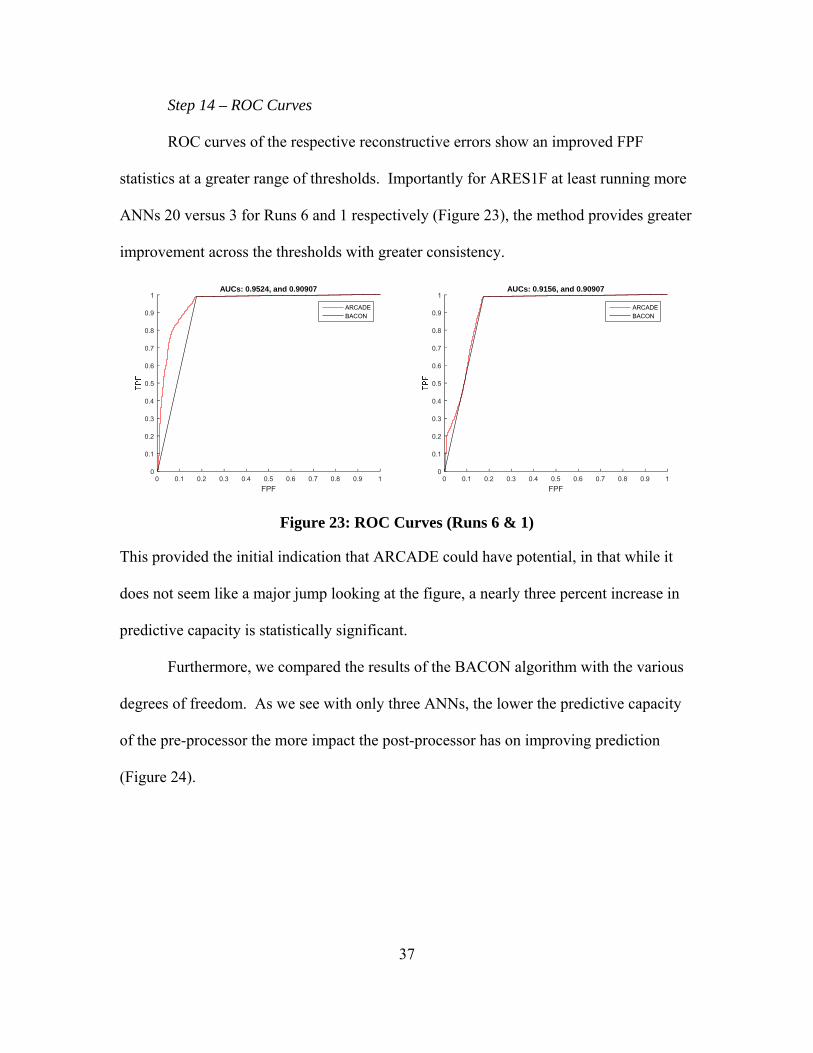
Step 14 – ROC Curves
ROC curves of the respective reconstructive errors show an improved FPF
statistics at a greater range of thresholds. Importantly for ARES1F at least running more
ANNs 20 versus 3 for Runs 6 and 1 respectively (Figure 23), the method provides greater
improvement across the thresholds with greater consistency.
Figure 23: ROC Curves (Runs 6 & 1)
This provided the initial indication that ARCADE could have potential, in that while it
does not seem like a major jump looking at the figure, a nearly three percent increase in
predictive capacity is statistically significant.
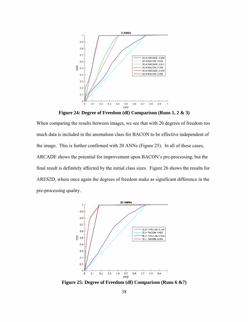
Furthermore, we compared the results of the BACON algorithm with the various
degrees of freedom. As we see with only three ANNs, the lower the predictive capacity
of the pre-processor the more impact the post-processor has on improving prediction
(Figure 24).
FPF0 0.1 0.2 0.3 0.4 0.5 0.6 0.7 0.8 0.9 1
0
0.1
0.2
0.3
0.4
0.5
0.6
0.7
0.8
0.9
1AUCs: 0.9524, and 0.90907
ARCADEBACON
FPF0 0.1 0.2 0.3 0.4 0.5 0.6 0.7 0.8 0.9 1
0
0.1
0.2
0.3
0.4
0.5
0.6
0.7
0.8
0.9
1AUCs: 0.9156, and 0.90907
ARCADEBACON
38
Figure 24: Degree of Freedom (df) Comparison (Runs 1, 2 & 3)
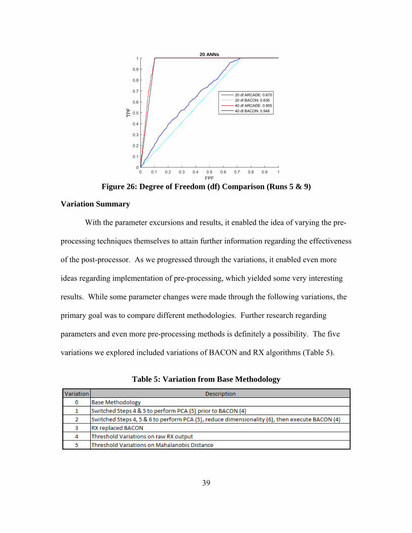
When comparing the results between images, we see that with 20 degrees of freedom too
much data is included in the anomalous class for BACON to be effective independent of
the image. This is further confirmed with 20 ANNs (Figure 25). In all of these cases,
ARCADE shows the potential for improvement upon BACON’s pre-processing, but the
final result is definitely affected by the initial class sizes. Figure 26 shows the results for
ARES2D, where once again the degrees of freedom make as significant difference in the
pre-processing quality.
Figure 25: Degree of Freedom (df) Comparison (Runs 6 &7)
FPF0 0.1 0.2 0.3 0.4 0.5 0.6 0.7 0.8 0.9 1
0
0.1
0.2
0.3
0.4
0.5
0.6
0.7
0.8
0.9
13 ANNs
20 df ARCADE: 0.68620 df BACON: 0.63230 df ARCADE: 0.81130 df BACON: 0.79440 df ARCADE: 0.91640 df BACON: 0.909
TPF
39
Figure 26: Degree of Freedom (df) Comparison (Runs 5 & 9)
Variation Summary
With the parameter excursions and results, it enabled the idea of varying the pre-
processing techniques themselves to attain further information regarding the effectiveness
of the post-processor. As we progressed through the variations, it enabled even more
ideas regarding implementation of pre-processing, which yielded some very interesting
results. While some parameter changes were made through the following variations, the
primary goal was to compare different methodologies. Further research regarding
parameters and even more pre-processing methods is definitely a possibility. The five
variations we explored included variations of BACON and RX algorithms (Table 5).
Table 5: Variation from Base Methodology
FPF0 0.1 0.2 0.3 0.4 0.5 0.6 0.7 0.8 0.9 1
0
0.1
0.2
0.3
0.4
0.5
0.6
0.7
0.8
0.9
120 ANNs
20 df ARCADE: 0.67020 df BACON: 0.63640 df ARCADE: 0.95540 df BACON: 0.948
40
Methodology Variation 1
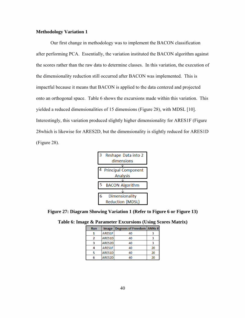
Our first change in methodology was to implement the BACON classification
after performing PCA. Essentially, the variation instituted the BACON algorithm against
the scores rather than the raw data to determine classes. In this variation, the execution of
the dimensionality reduction still occurred after BACON was implemented. This is
impactful because it means that BACON is applied to the data centered and projected
onto an orthogonal space. Table 6 shows the excursions made within this variation. This
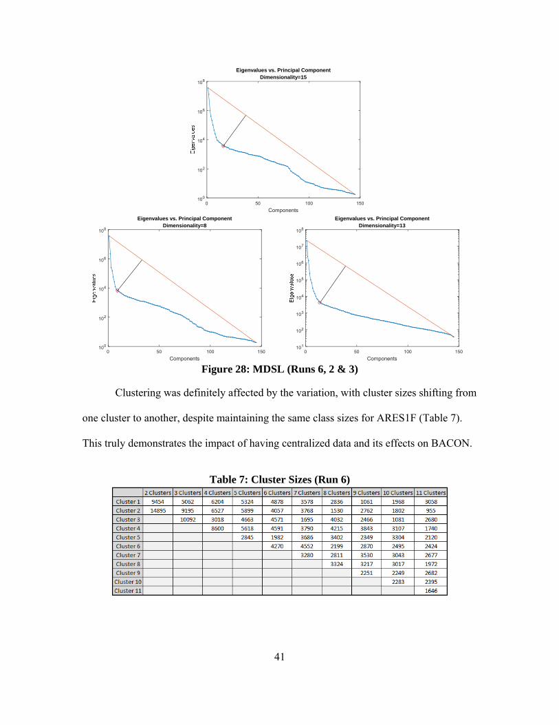
yielded a reduced dimensionalities of 15 dimensions (Figure 28), with MDSL [10].
Interestingly, this variation produced slightly higher dimensionality for ARES1F (Figure
28which is likewise for ARES2D, but the dimensionality is slightly reduced for ARES1D
(Figure 28).
Figure 27: Diagram Showing Variation 1 (Refer to Figure 6 or Figure 13)
Table 6: Image & Parameter Excursions (Using Scores Matrix)
41
Figure 28: MDSL (Runs 6, 2 & 3)
Clustering was definitely affected by the variation, with cluster sizes shifting from
one cluster to another, despite maintaining the same class sizes for ARES1F (Table 7).
This truly demonstrates the impact of having centralized data and its effects on BACON.
Table 7: Cluster Sizes (Run 6)
Components0 50 100 150
100
102
104
106
108
Eigenvalues vs. Principal ComponentDimensionality=15
Components0 50 100 150
100
102
104
106
108
Eigenvalues vs. Principal ComponentDimensionality=8
Components0 50 100 150
101
102
103
104
105
106
107
108
Eigenvalues vs. Principal ComponentDimensionality=13
42
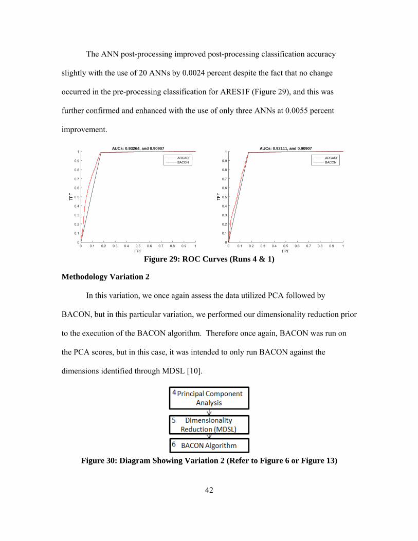
The ANN post-processing improved post-processing classification accuracy
slightly with the use of 20 ANNs by 0.0024 percent despite the fact that no change
occurred in the pre-processing classification for ARES1F (Figure 29), and this was
further confirmed and enhanced with the use of only three ANNs at 0.0055 percent
improvement.
Figure 29: ROC Curves (Runs 4 & 1)
Methodology Variation 2
In this variation, we once again assess the data utilized PCA followed by
BACON, but in this particular variation, we performed our dimensionality reduction prior
to the execution of the BACON algorithm. Therefore once again, BACON was run on
the PCA scores, but in this case, it was intended to only run BACON against the
dimensions identified through MDSL [10].
Figure 30: Diagram Showing Variation 2 (Refer to Figure 6 or Figure 13)
FPF0 0.1 0.2 0.3 0.4 0.5 0.6 0.7 0.8 0.9 1
0
0.1
0.2
0.3
0.4
0.5
0.6
0.7
0.8
0.9
1AUCs: 0.93264, and 0.90907
ARCADEBACON
FPF0 0.1 0.2 0.3 0.4 0.5 0.6 0.7 0.8 0.9 1
0
0.1
0.2
0.3
0.4
0.5
0.6
0.7
0.8
0.9
1AUCs: 0.92111, and 0.90907
ARCADEBACON
43
However, upon attempting this variation with the parameters associated with
BACON for the previous runs, we were not able to execute the subsequent clustering
because the class size of the anomalous class was too small or in some cases non-existent.
Thus, we substantially adjusted three of the parameters. Notably, some adjustments led
to all data observations being sent to the anomalous class, while leaving the background
class empty. First, we made adjustments to the alpha values associated with the Chi-
Squared test utilized in BACON. Previous runs had applied an alpha of 0.05, this was
modified to span between 0.1 and 0.5. Second, we adjusted the degrees of freedom.
Other experimentation had degrees of freedom ranging from 20 to 40; with this variation,
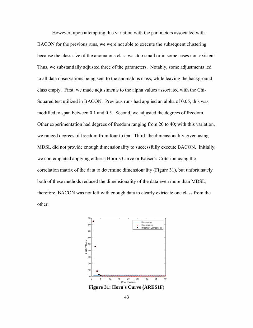
we ranged degrees of freedom from four to ten. Third, the dimensionality given using
MDSL did not provide enough dimensionality to successfully execute BACON. Initially,
we contemplated applying either a Horn’s Curve or Kaiser’s Criterion using the
correlation matrix of the data to determine dimensionality (Figure 31), but unfortunately
both of these methods reduced the dimensionality of the data even more than MDSL;
therefore, BACON was not left with enough data to clearly extricate one class from the
other.
Figure 31: Horn's Curve (ARES1F)
Components0 5 10 15 20 25 30 35 40
0
10
20
30
40
50
60
70
80
90
HornscurveEigenvaluesImportant Components

44
Learning this, we experimented with an added dimensionality ranging from an
additional 20 to an additional 50 dimensions. Again it is critical to note that in some
cases, these parameter varieties did not include all of the known anomalies and in others
they sent so much of the image data into the anomalous class that it did not have a
positive effect. Based on these findings, we tried a variety of parameter combinations to
see what the differences would be as the parameters shifted. Generally speaking, we saw
some improved performance using our post-processing methodology, but we did not see
across the board quality results with any specific set of parameter settings across the
various images.
For ARES1F, we compared four different parameter settings (Table 8), but while our
method showed demonstrable improvement over the BACON class identification
accuracy, BACON’s predictive capacity for this image given the reduced dimensionality
was extremely poor. Therefore even with our improved performance, the performance
regarding this image was poor. One sees that BACON never achieves a classification
rate much better than the flip of a coin (Figure 32). The best result of our method comes
when the parameter settings are at their middle points, but the second best performance
comes when the parameter settings were at their lowest points, leaving a lot to be
discovered.
45
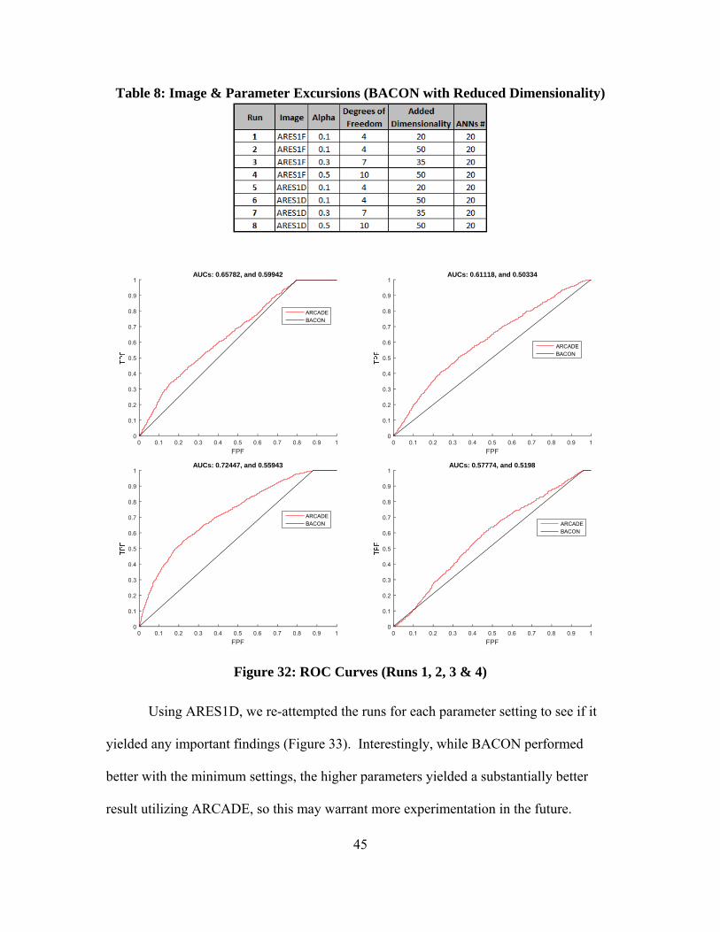
Table 8: Image & Parameter Excursions (BACON with Reduced Dimensionality)
Figure 32: ROC Curves (Runs 1, 2, 3 & 4)
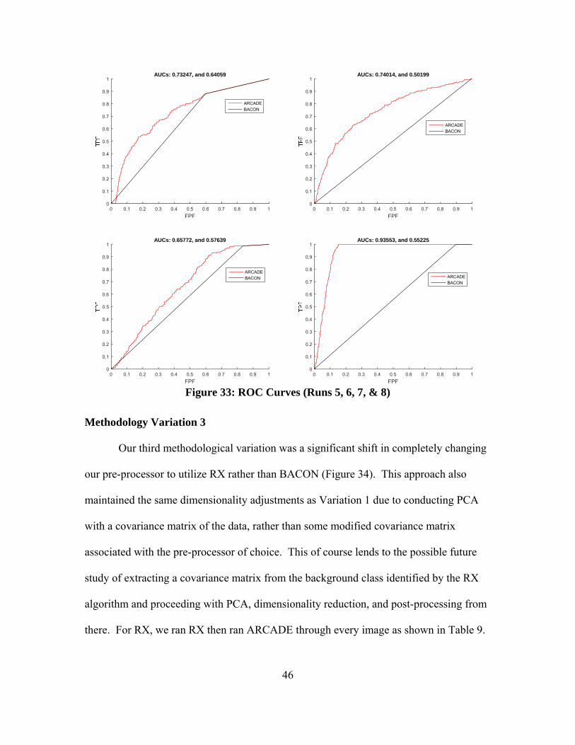
Using ARES1D, we re-attempted the runs for each parameter setting to see if it
yielded any important findings (Figure 33). Interestingly, while BACON performed
better with the minimum settings, the higher parameters yielded a substantially better
result utilizing ARCADE, so this may warrant more experimentation in the future.
FPF0 0.1 0.2 0.3 0.4 0.5 0.6 0.7 0.8 0.9 1
0
0.1
0.2
0.3
0.4
0.5
0.6
0.7
0.8
0.9
1AUCs: 0.65782, and 0.59942
ARCADEBACON
FPF0 0.1 0.2 0.3 0.4 0.5 0.6 0.7 0.8 0.9 1
0
0.1
0.2
0.3
0.4
0.5
0.6
0.7
0.8
0.9
1AUCs: 0.61118, and 0.50334
ARCADEBACON
FPF0 0.1 0.2 0.3 0.4 0.5 0.6 0.7 0.8 0.9 1
0
0.1
0.2
0.3
0.4
0.5
0.6
0.7
0.8
0.9
1AUCs: 0.72447, and 0.55943
ARCADEBACON
FPF0 0.1 0.2 0.3 0.4 0.5 0.6 0.7 0.8 0.9 1
0
0.1
0.2
0.3
0.4
0.5
0.6
0.7
0.8
0.9
1AUCs: 0.57774, and 0.5198
ARCADEBACON
46
Figure 33: ROC Curves (Runs 5, 6, 7, & 8)
Methodology Variation 3
Our third methodological variation was a significant shift in completely changing
our pre-processor to utilize RX rather than BACON (Figure 34). This approach also
maintained the same dimensionality adjustments as Variation 1 due to conducting PCA
with a covariance matrix of the data, rather than some modified covariance matrix
associated with the pre-processor of choice. This of course lends to the possible future
study of extracting a covariance matrix from the background class identified by the RX
algorithm and proceeding with PCA, dimensionality reduction, and post-processing from
there. For RX, we ran RX then ran ARCADE through every image as shown in Table 9.
FPF0 0.1 0.2 0.3 0.4 0.5 0.6 0.7 0.8 0.9 1
0
0.1
0.2
0.3
0.4
0.5
0.6
0.7
0.8
0.9
1AUCs: 0.73247, and 0.64059
ARCADEBACON
FPF0 0.1 0.2 0.3 0.4 0.5 0.6 0.7 0.8 0.9 1
0
0.1
0.2
0.3
0.4
0.5
0.6
0.7
0.8
0.9
1AUCs: 0.74014, and 0.50199
ARCADEBACON
FPF0 0.1 0.2 0.3 0.4 0.5 0.6 0.7 0.8 0.9 1
0
0.1
0.2
0.3
0.4
0.5
0.6
0.7
0.8
0.9
1AUCs: 0.65772, and 0.57639
ARCADEBACON
FPF0 0.1 0.2 0.3 0.4 0.5 0.6 0.7 0.8 0.9 1
0
0.1
0.2
0.3
0.4
0.5
0.6
0.7
0.8
0.9
1AUCs: 0.93553, and 0.55225
ARCADEBACON
47
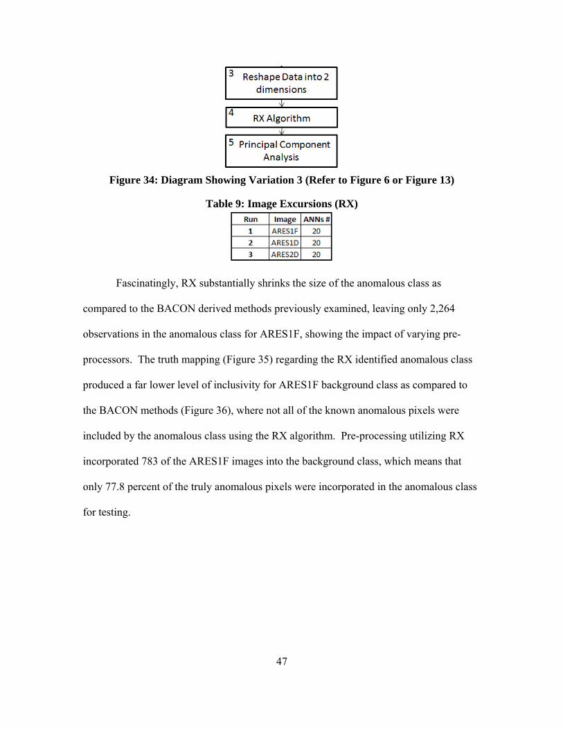
Figure 34: Diagram Showing Variation 3 (Refer to Figure 6 or Figure 13)
Table 9: Image Excursions (RX)
Fascinatingly, RX substantially shrinks the size of the anomalous class as
compared to the BACON derived methods previously examined, leaving only 2,264
observations in the anomalous class for ARES1F, showing the impact of varying pre-
processors. The truth mapping (Figure 35) regarding the RX identified anomalous class
produced a far lower level of inclusivity for ARES1F background class as compared to
the BACON methods (Figure 36), where not all of the known anomalous pixels were
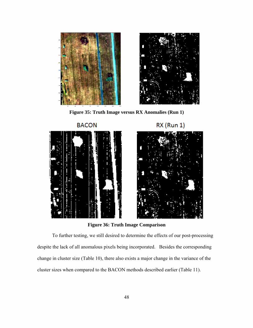
included by the anomalous class using the RX algorithm. Pre-processing utilizing RX
incorporated 783 of the ARES1F images into the background class, which means that
only 77.8 percent of the truly anomalous pixels were incorporated in the anomalous class
for testing.
48
Figure 35: Truth Image versus RX Anomalies (Run 1)
Figure 36: Truth Image Comparison
To further testing, we still desired to determine the effects of our post-processing
despite the lack of all anomalous pixels being incorporated. Besides the corresponding
change in cluster size (Table 10), there also exists a major change in the variance of the
cluster sizes when compared to the BACON methods described earlier (Table 11).
49
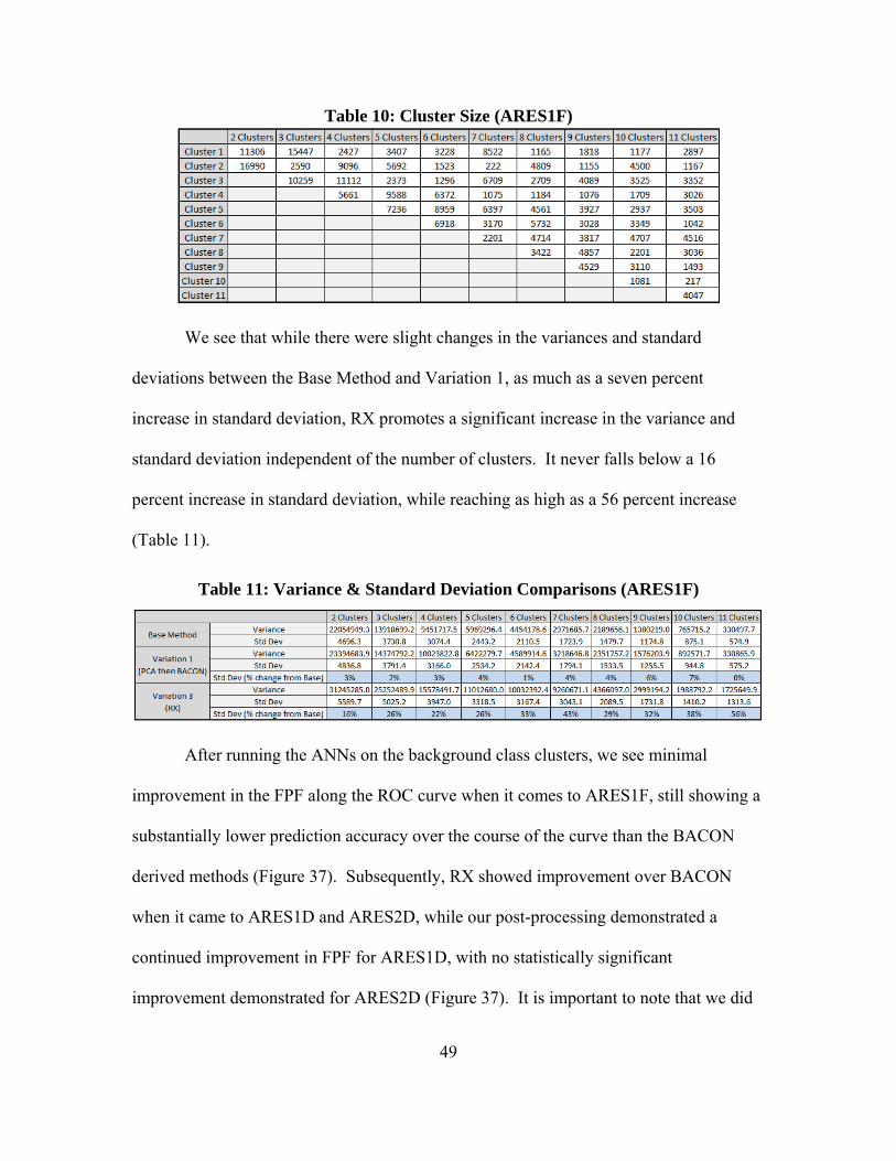
Table 10: Cluster Size (ARES1F)
We see that while there were slight changes in the variances and standard
deviations between the Base Method and Variation 1, as much as a seven percent
increase in standard deviation, RX promotes a significant increase in the variance and
standard deviation independent of the number of clusters. It never falls below a 16
percent increase in standard deviation, while reaching as high as a 56 percent increase
(Table 11).
Table 11: Variance & Standard Deviation Comparisons (ARES1F)
After running the ANNs on the background class clusters, we see minimal
improvement in the FPF along the ROC curve when it comes to ARES1F, still showing a
substantially lower prediction accuracy over the course of the curve than the BACON
derived methods (Figure 37). Subsequently, RX showed improvement over BACON
when it came to ARES1D and ARES2D, while our post-processing demonstrated a
continued improvement in FPF for ARES1D, with no statistically significant
improvement demonstrated for ARES2D (Figure 37). It is important to note that we did
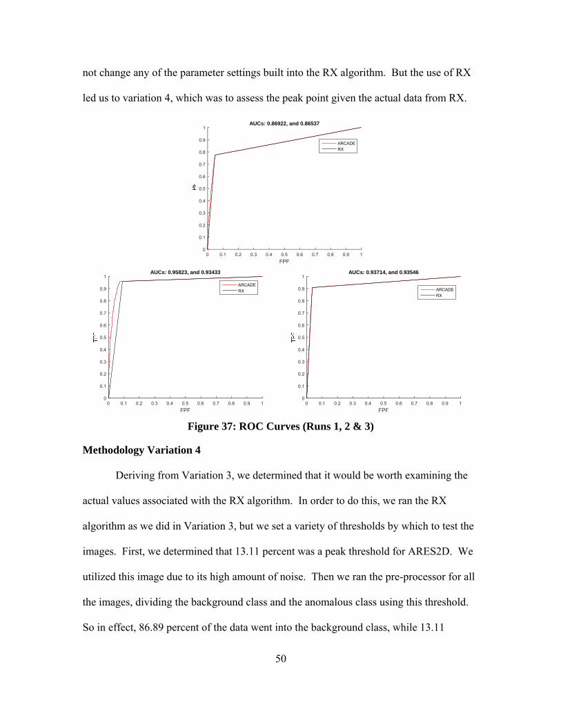
50
not change any of the parameter settings built into the RX algorithm. But the use of RX
led us to variation 4, which was to assess the peak point given the actual data from RX.
Figure 37: ROC Curves (Runs 1, 2 & 3)
Methodology Variation 4
Deriving from Variation 3, we determined that it would be worth examining the
actual values associated with the RX algorithm. In order to do this, we ran the RX
algorithm as we did in Variation 3, but we set a variety of thresholds by which to test the
images. First, we determined that 13.11 percent was a peak threshold for ARES2D. We
utilized this image due to its high amount of noise. Then we ran the pre-processor for all
the images, dividing the background class and the anomalous class using this threshold.
So in effect, 86.89 percent of the data went into the background class, while 13.11
FPF0 0.1 0.2 0.3 0.4 0.5 0.6 0.7 0.8 0.9 1
0
0.1
0.2
0.3
0.4
0.5
0.6
0.7
0.8
0.9
1AUCs: 0.86922, and 0.86537
ARCADERX
FPF0 0.1 0.2 0.3 0.4 0.5 0.6 0.7 0.8 0.9 1
0
0.1
0.2
0.3
0.4
0.5
0.6
0.7
0.8
0.9
1AUCs: 0.95823, and 0.93433
ARCADERX
FPF0 0.1 0.2 0.3 0.4 0.5 0.6 0.7 0.8 0.9 1
0
0.1
0.2
0.3
0.4
0.5
0.6
0.7
0.8
0.9
1AUCs: 0.93714, and 0.93546
ARCADERX
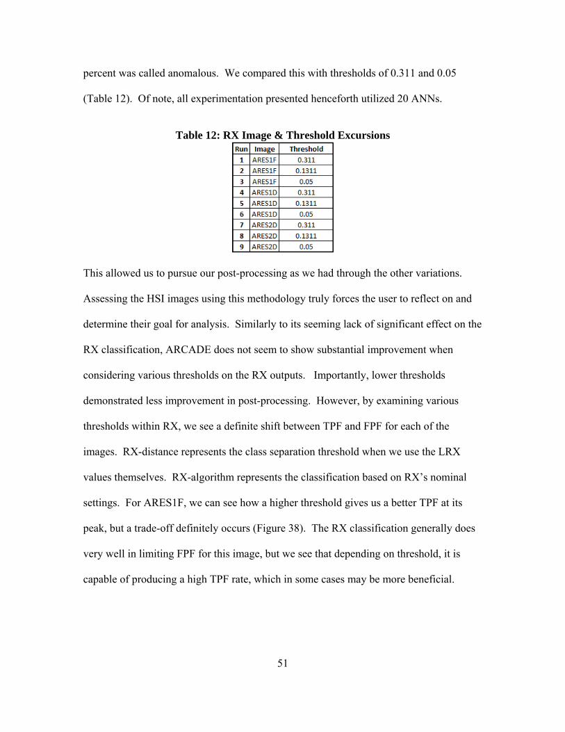
51
percent was called anomalous. We compared this with thresholds of 0.311 and 0.05
(Table 12). Of note, all experimentation presented henceforth utilized 20 ANNs.
Table 12: RX Image & Threshold Excursions
This allowed us to pursue our post-processing as we had through the other variations.
Assessing the HSI images using this methodology truly forces the user to reflect on and
determine their goal for analysis. Similarly to its seeming lack of significant effect on the
RX classification, ARCADE does not seem to show substantial improvement when
considering various thresholds on the RX outputs. Importantly, lower thresholds
demonstrated less improvement in post-processing. However, by examining various
thresholds within RX, we see a definite shift between TPF and FPF for each of the
images. RX-distance represents the class separation threshold when we use the LRX
values themselves. RX-algorithm represents the classification based on RX’s nominal
settings. For ARES1F, we can see how a higher threshold gives us a better TPF at its
peak, but a trade-off definitely occurs (Figure 38). The RX classification generally does
very well in limiting FPF for this image, but we see that depending on threshold, it is
capable of producing a high TPF rate, which in some cases may be more beneficial.
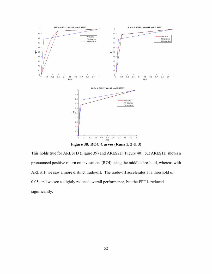
52
Figure 38: ROC Curves (Runs 1, 2 & 3)
This holds true for ARES1D (Figure 39) and ARES2D (Figure 40), but ARES1D shows a
pronounced positive return on investment (ROI) using the middle threshold, whereas with
ARES1F we saw a more distinct trade-off. The trade-off accelerates at a threshold of
0.05, and we see a slightly reduced overall performance, but the FPF is reduced
significantly.
FPF0 0.1 0.2 0.3 0.4 0.5 0.6 0.7 0.8 0.9 1
0
0.1
0.2
0.3
0.4
0.5
0.6
0.7
0.8
0.9
1AUCs: 0.8722, 0.8334, and 0.86537
ARCADERX-distanceRX-algorithm
FPF0 0.1 0.2 0.3 0.4 0.5 0.6 0.7 0.8 0.9 1
0
0.1
0.2
0.3
0.4
0.5
0.6
0.7
0.8
0.9
1AUCs: 0.90395, 0.89055, and 0.86537
ARCADERX-distanceRX-algorithm
FPF0 0.1 0.2 0.3 0.4 0.5 0.6 0.7 0.8 0.9 1
0
0.1
0.2
0.3
0.4
0.5
0.6
0.7
0.8
0.9
1AUCs: 0.81937, 0.8188, and 0.86537
ARCADERX-distanceRX-algorithm
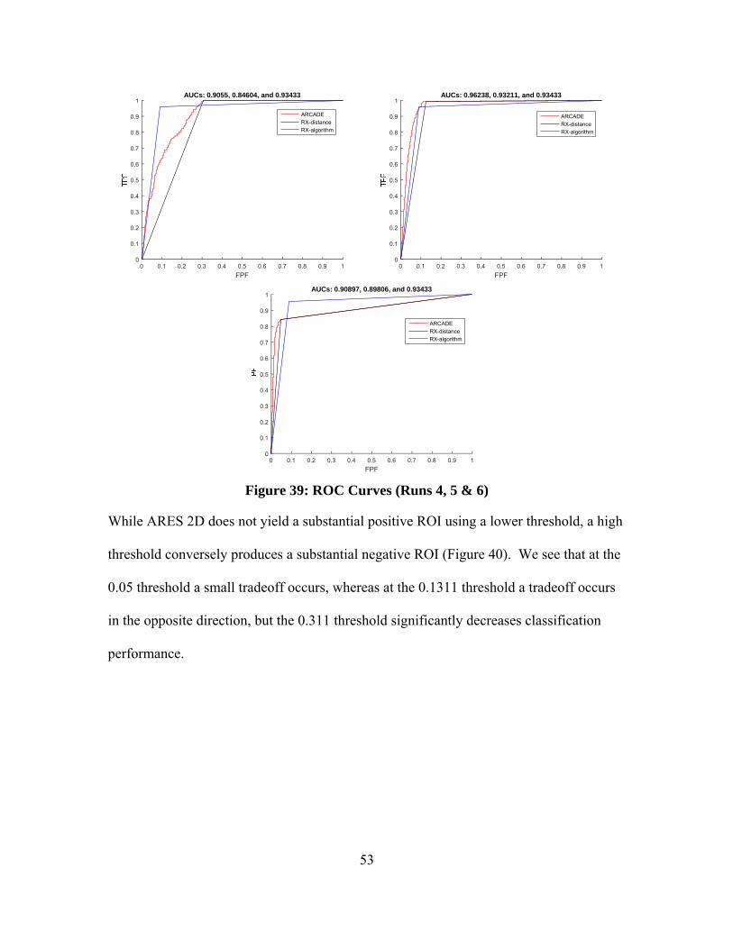
53
Figure 39: ROC Curves (Runs 4, 5 & 6)
While ARES 2D does not yield a substantial positive ROI using a lower threshold, a high
threshold conversely produces a substantial negative ROI (Figure 40). We see that at the
0.05 threshold a small tradeoff occurs, whereas at the 0.1311 threshold a tradeoff occurs
in the opposite direction, but the 0.311 threshold significantly decreases classification
performance.
FPF0 0.1 0.2 0.3 0.4 0.5 0.6 0.7 0.8 0.9 1
0
0.1
0.2
0.3
0.4
0.5
0.6
0.7
0.8
0.9
1AUCs: 0.9055, 0.84604, and 0.93433
ARCADERX-distanceRX-algorithm
FPF0 0.1 0.2 0.3 0.4 0.5 0.6 0.7 0.8 0.9 1
0
0.1
0.2
0.3
0.4
0.5
0.6
0.7
0.8
0.9
1AUCs: 0.96238, 0.93211, and 0.93433
ARCADERX-distanceRX-algorithm
FPF0 0.1 0.2 0.3 0.4 0.5 0.6 0.7 0.8 0.9 1
0
0.1
0.2
0.3
0.4
0.5
0.6
0.7
0.8
0.9
1AUCs: 0.90897, 0.89806, and 0.93433
ARCADERX-distanceRX-algorithm
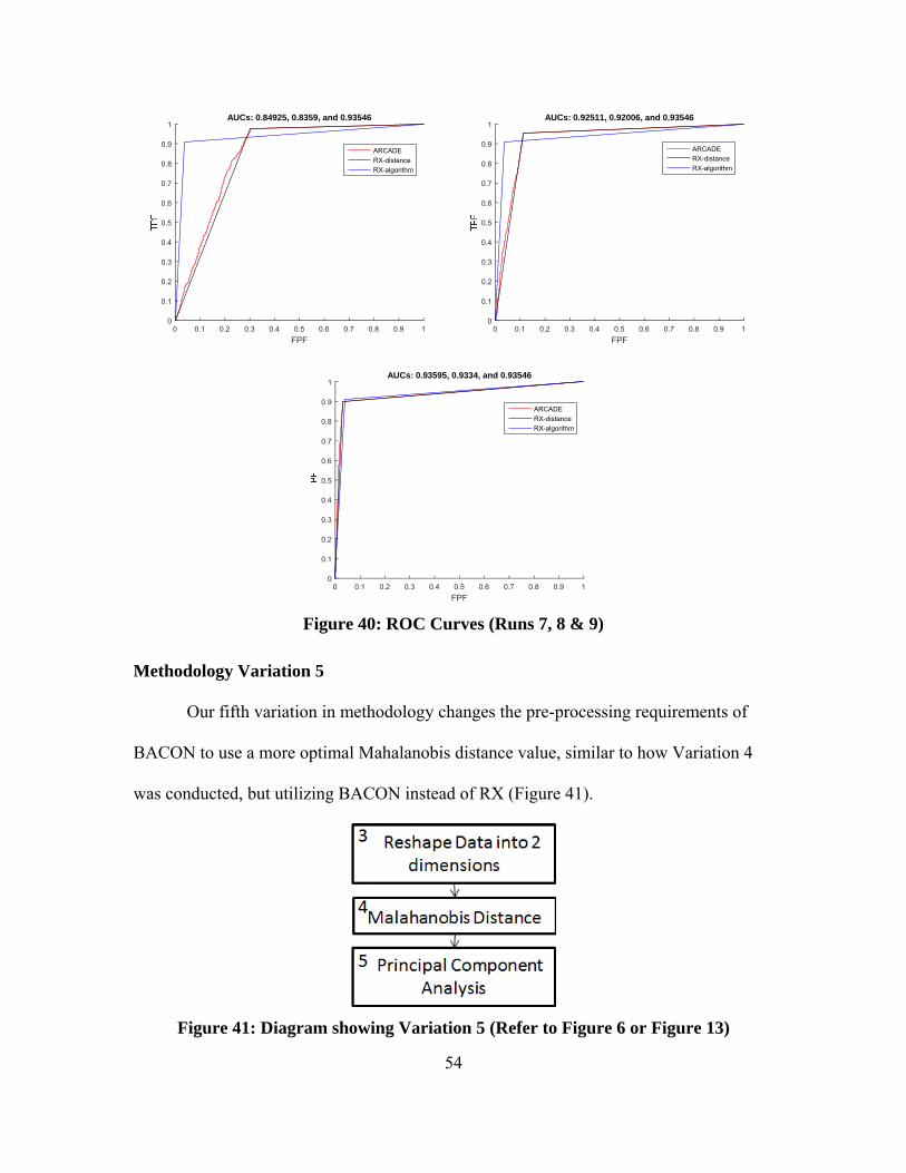
54
Figure 40: ROC Curves (Runs 7, 8 & 9)
Methodology Variation 5
Our fifth variation in methodology changes the pre-processing requirements of
BACON to use a more optimal Mahalanobis distance value, similar to how Variation 4
was conducted, but utilizing BACON instead of RX (Figure 41).
Figure 41: Diagram showing Variation 5 (Refer to Figure 6 or Figure 13)
FPF0 0.1 0.2 0.3 0.4 0.5 0.6 0.7 0.8 0.9 1
0
0.1
0.2
0.3
0.4
0.5
0.6
0.7
0.8
0.9
1AUCs: 0.84925, 0.8359, and 0.93546
ARCADERX-distanceRX-algorithm
FPF0 0.1 0.2 0.3 0.4 0.5 0.6 0.7 0.8 0.9 1
0
0.1
0.2
0.3
0.4
0.5
0.6
0.7
0.8
0.9
1AUCs: 0.92511, 0.92006, and 0.93546
ARCADERX-distanceRX-algorithm
FPF0 0.1 0.2 0.3 0.4 0.5 0.6 0.7 0.8 0.9 1
0
0.1
0.2
0.3
0.4
0.5
0.6
0.7
0.8
0.9
1AUCs: 0.93595, 0.9334, and 0.93546
ARCADERX-distanceRX-algorithm
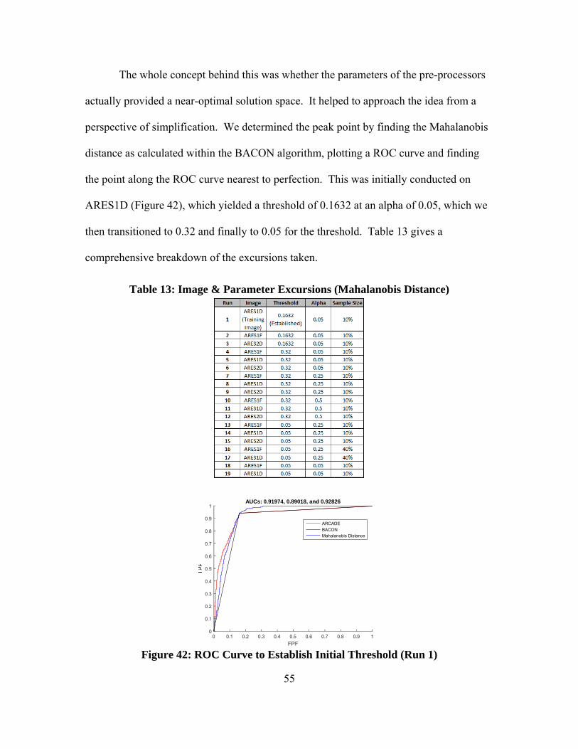
55
The whole concept behind this was whether the parameters of the pre-processors
actually provided a near-optimal solution space. It helped to approach the idea from a
perspective of simplification. We determined the peak point by finding the Mahalanobis
distance as calculated within the BACON algorithm, plotting a ROC curve and finding
the point along the ROC curve nearest to perfection. This was initially conducted on
ARES1D (Figure 42), which yielded a threshold of 0.1632 at an alpha of 0.05, which we
then transitioned to 0.32 and finally to 0.05 for the threshold. Table 13 gives a
comprehensive breakdown of the excursions taken.
Table 13: Image & Parameter Excursions (Mahalanobis Distance)
Figure 42: ROC Curve to Establish Initial Threshold (Run 1)
FPF0 0.1 0.2 0.3 0.4 0.5 0.6 0.7 0.8 0.9 1
0
0.1
0.2
0.3
0.4
0.5
0.6
0.7
0.8
0.9
1AUCs: 0.91974, 0.89018, and 0.92826
ARCADEBACONMahalanobis Distance
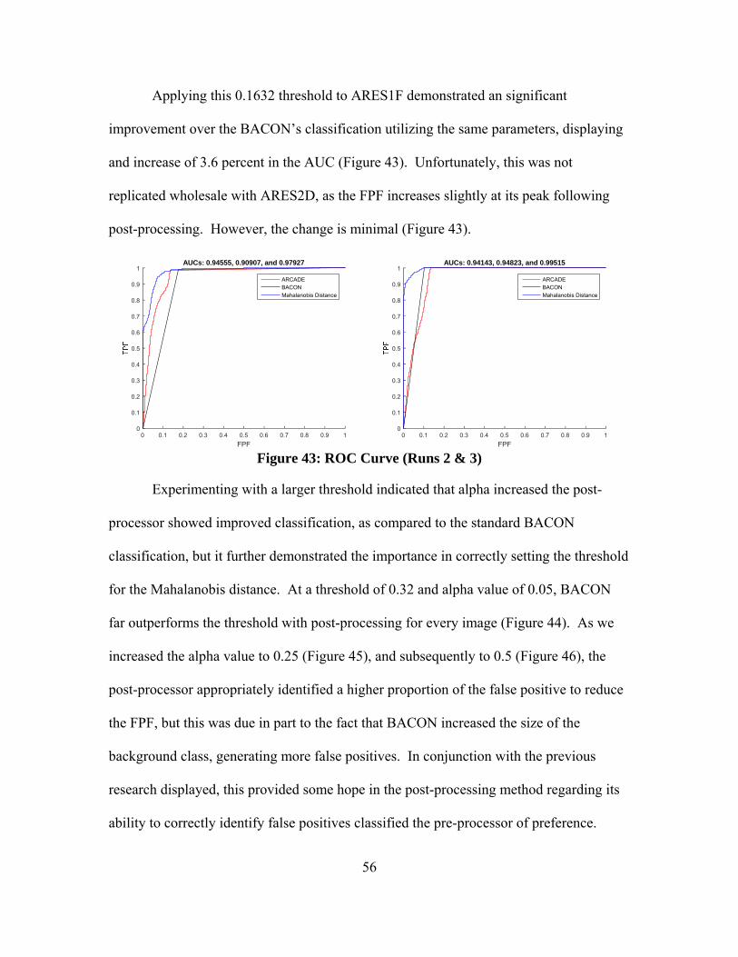
56
Applying this 0.1632 threshold to ARES1F demonstrated an significant
improvement over the BACON’s classification utilizing the same parameters, displaying
and increase of 3.6 percent in the AUC (Figure 43). Unfortunately, this was not
replicated wholesale with ARES2D, as the FPF increases slightly at its peak following
post-processing. However, the change is minimal (Figure 43).
Figure 43: ROC Curve (Runs 2 & 3)
Experimenting with a larger threshold indicated that alpha increased the post-
processor showed improved classification, as compared to the standard BACON
classification, but it further demonstrated the importance in correctly setting the threshold
for the Mahalanobis distance. At a threshold of 0.32 and alpha value of 0.05, BACON
far outperforms the threshold with post-processing for every image (Figure 44). As we
increased the alpha value to 0.25 (Figure 45), and subsequently to 0.5 (Figure 46), the
post-processor appropriately identified a higher proportion of the false positive to reduce
the FPF, but this was due in part to the fact that BACON increased the size of the
background class, generating more false positives. In conjunction with the previous
research displayed, this provided some hope in the post-processing method regarding its
ability to correctly identify false positives classified the pre-processor of preference.
FPF0 0.1 0.2 0.3 0.4 0.5 0.6 0.7 0.8 0.9 1
0
0.1
0.2
0.3
0.4
0.5
0.6
0.7
0.8
0.9
1AUCs: 0.94555, 0.90907, and 0.97927
ARCADEBACONMahalanobis Distance
FPF0 0.1 0.2 0.3 0.4 0.5 0.6 0.7 0.8 0.9 1
0
0.1
0.2
0.3
0.4
0.5
0.6
0.7
0.8
0.9
1AUCs: 0.94143, 0.94823, and 0.99515
ARCADEBACONMahalanobis Distance
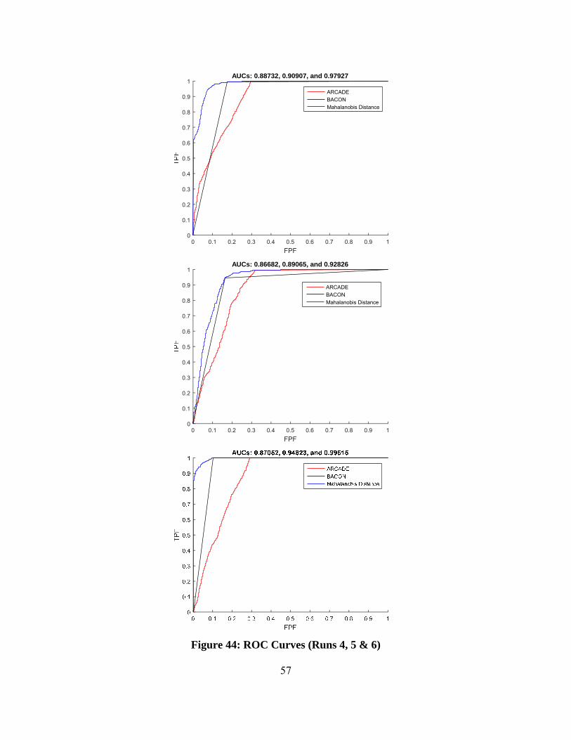
57
Figure 44: ROC Curves (Runs 4, 5 & 6)
FPF0 0.1 0.2 0.3 0.4 0.5 0.6 0.7 0.8 0.9 1
0
0.1
0.2
0.3
0.4
0.5
0.6
0.7
0.8
0.9
1AUCs: 0.88732, 0.90907, and 0.97927
ARCADEBACONMahalanobis Distance
FPF0 0.1 0.2 0.3 0.4 0.5 0.6 0.7 0.8 0.9 1
0
0.1
0.2
0.3
0.4
0.5
0.6
0.7
0.8
0.9
1AUCs: 0.86682, 0.89065, and 0.92826
ARCADEBACONMahalanobis Distance
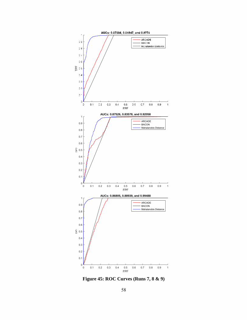
58
Figure 45: ROC Curves (Runs 7, 8 & 9)
TPF
FPF0 0.1 0.2 0.3 0.4 0.5 0.6 0.7 0.8 0.9 1
0
0.1
0.2
0.3
0.4
0.5
0.6
0.7
0.8
0.9
1AUCs: 0.87526, 0.83578, and 0.92058
ARCADEBACONMahalanobis Distance
FPF0 0.1 0.2 0.3 0.4 0.5 0.6 0.7 0.8 0.9 1
0
0.1
0.2
0.3
0.4
0.5
0.6
0.7
0.8
0.9
1AUCs: 0.86805, 0.88939, and 0.99488
ARCADEBACONMahalanobis Distance
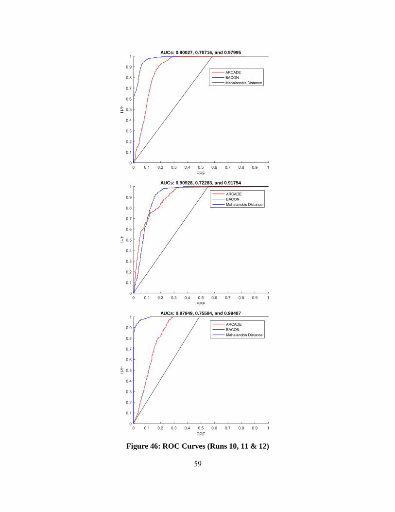
59
Figure 46: ROC Curves (Runs 10, 11 & 12)
FPF0 0.1 0.2 0.3 0.4 0.5 0.6 0.7 0.8 0.9 1
0
0.1
0.2
0.3
0.4
0.5
0.6
0.7
0.8
0.9
1AUCs: 0.90027, 0.70716, and 0.97995
ARCADEBACONMahalanobis Distance
FPF0 0.1 0.2 0.3 0.4 0.5 0.6 0.7 0.8 0.9 1
0
0.1
0.2
0.3
0.4
0.5
0.6
0.7
0.8
0.9
1AUCs: 0.90928, 0.72283, and 0.91754
ARCADEBACONMahalanobis Distance
FPF0 0.1 0.2 0.3 0.4 0.5 0.6 0.7 0.8 0.9 1
0
0.1
0.2
0.3
0.4
0.5
0.6
0.7
0.8
0.9
1AUCs: 0.87949, 0.75584, and 0.99487
ARCADEBACONMahalanobis Distance
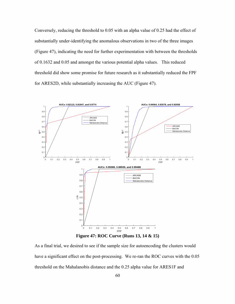
60
Conversely, reducing the threshold to 0.05 with an alpha value of 0.25 had the effect of
substantially under-identifying the anomalous observations in two of the three images
(Figure 47), indicating the need for further experimentation with between the thresholds
of 0.1632 and 0.05 and amongst the various potential alpha values. This reduced
threshold did show some promise for future research as it substantially reduced the FPF
for ARES2D, while substantially increasing the AUC (Figure 47).
Figure 47: ROC Curve (Runs 13, 14 & 15)
As a final trial, we desired to see if the sample size for autoencoding the clusters would
have a significant effect on the post-processing. We re-ran the ROC curves with the 0.05
threshold on the Mahalanobis distance and the 0.25 alpha value for ARES1F and
FPF0 0.1 0.2 0.3 0.4 0.5 0.6 0.7 0.8 0.9 1
0
0.1
0.2
0.3
0.4
0.5
0.6
0.7
0.8
0.9
1AUCs: 0.82115, 0.81947, and 0.9774
ARCADEBACONMahalanobis Distance
FPF0 0.1 0.2 0.3 0.4 0.5 0.6 0.7 0.8 0.9 1
0
0.1
0.2
0.3
0.4
0.5
0.6
0.7
0.8
0.9
1AUCs: 0.66064, 0.83578, and 0.92058
ARCADEBACONMahalanobis Distance
FPF0 0.1 0.2 0.3 0.4 0.5 0.6 0.7 0.8 0.9 1
0
0.1
0.2
0.3
0.4
0.5
0.6
0.7
0.8
0.9
1AUCs: 0.95589, 0.88939, and 0.99488
ARCADEBACONMahalanobis Distance
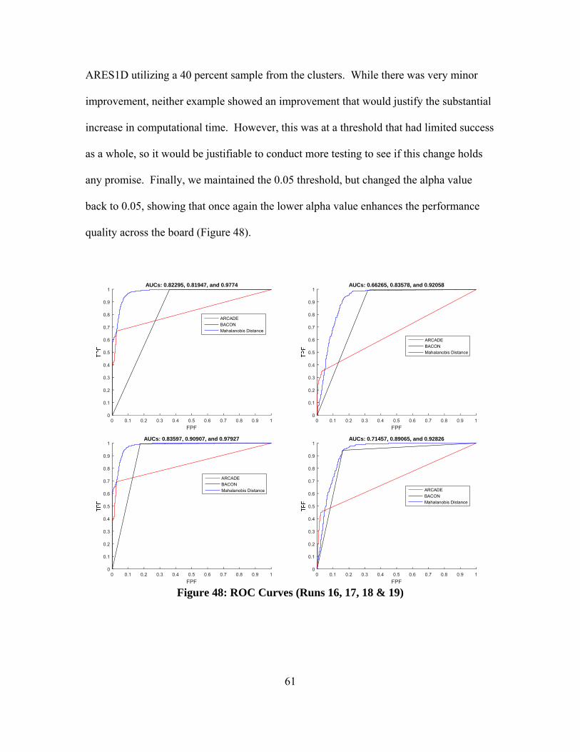
61
ARES1D utilizing a 40 percent sample from the clusters. While there was very minor
improvement, neither example showed an improvement that would justify the substantial
increase in computational time. However, this was at a threshold that had limited success
as a whole, so it would be justifiable to conduct more testing to see if this change holds
any promise. Finally, we maintained the 0.05 threshold, but changed the alpha value
back to 0.05, showing that once again the lower alpha value enhances the performance
quality across the board (Figure 48).
Figure 48: ROC Curves (Runs 16, 17, 18 & 19)
FPF0 0.1 0.2 0.3 0.4 0.5 0.6 0.7 0.8 0.9 1
0
0.1
0.2
0.3
0.4
0.5
0.6
0.7
0.8
0.9
1AUCs: 0.82295, 0.81947, and 0.9774
ARCADEBACONMahalanobis Distance
FPF0 0.1 0.2 0.3 0.4 0.5 0.6 0.7 0.8 0.9 1
0
0.1
0.2
0.3
0.4
0.5
0.6
0.7
0.8
0.9
1AUCs: 0.66265, 0.83578, and 0.92058
ARCADEBACONMahalanobis Distance
FPF0 0.1 0.2 0.3 0.4 0.5 0.6 0.7 0.8 0.9 1
0
0.1
0.2
0.3
0.4
0.5
0.6
0.7
0.8
0.9
1AUCs: 0.83597, 0.90907, and 0.97927
ARCADEBACONMahalanobis Distance
FPF0 0.1 0.2 0.3 0.4 0.5 0.6 0.7 0.8 0.9 1
0
0.1
0.2
0.3
0.4
0.5
0.6
0.7
0.8
0.9
1AUCs: 0.71457, 0.89065, and 0.92826
ARCADEBACONMahalanobis Distance
62
Investigative Questions
We examined six different variations of our method (Figure 13). In these
variations, we compared two different pre-processors, two orders of processing and two
outputs from each of the pre-processors. In addition to the comparisons between the pre-
processors, we compared various parameter settings associated with those processors.
Furthermore in post-processing, we compared a variety of thresholds by which to
comparatively assess HYDICE images. This provided us with extensive scope into the
overall methodology to optimally determine parameter settings and methodology by
which to approach the analysis of HYDICE HSI images for classification and anomaly
detection.
All of this experimentation allowed us to explore the effectiveness of pre-
processing techniques, as well as the robustness of our post-processing method in
enhancing data classification post pre-processing. It is important to note, as verified by
experimentation, that our post-processing method really applies to reducing the FPF
produced by a pre-processor. The ANNs as we have applied them are unable to take data
that was pre-classified as background data and re-classify it as anomalous. This
emphasizes the importance of ensuring a quality problem definition. If the most
important thing is minimizing false positives, it may be reasonable for some of the true
anomalies to be classified as background data, as long as it is not to the extent that it
impinges upon the true classification of the background data. However, if the most
important thing is to find the anomalies, the true positives, then it is critical that any pre-
processing technique utilized pushes all of the true anomalies to the anomalous class,
63
while ensuring that the anomalous class is not so large as to make it nearly
indistinguishable from the background class.
Summary
We tested a variety of pre-processing methods with our post-processing
methodology, allowing for and making some parameter variations along the way. The
different pre-processing methods changed how the post-processor interacted with the data
sets, but this helped to gain insight into the overall validity of the post-processor as
applied to data pre-processed using a variety of techniques. It implied future research
and validity in applying this post-processing method to other pre-processors to further
reduce Type I error associated with the classification of anomalies within data.
Hopefully, in future research, we can enhance the number of true positives; thereby,
reducing false negatives as well. But we seemingly have had the most success thus far in
reducing the false positives associated with the Type I error. As we progress in this
research, there is ample promise for the enhancement of this process, recognizing that in
these images in particular, given the state of the world today, false positives are by far the
most negative outcome. Therefore, by enhancing our thresholds, parameters and
performance, we can amply improve performance in line with our desired outcome.
64
V. Conclusions and Recommendations
Chapter Overview
In assessing our base methodology, we observed some improved classification
accuracy with ARCADE, but this discovery also led us to examine other pre-possessing
possibilities. Originally, we executed BACON on the raw data. Our first and second
excursions were to assess ARCADE’s variance executing BACON on the principal
component scores, with full and reduced dimensionality. This was followed by the use of
the RX algorithm and finally evaluations based on the Mahalanobis distances. This use
of a variety of pre-processing techniques allowed us to experiment with ARCADE
Simultaneously, we experimented with parameter adjustments within the pre-processors
themselves.
In this chapter, we first provide a more in-depth examination of how the BACON
and RX algorithms interacted with the data, assessing their true ability in performing
anomaly detection. We assessed the algorithmic classification, as well as the values
which produced the partitioning of classes for the various algorithms. This allows us to
further examine the variations associated with both algorithms and both algorithms
outputs. Assessments across multiple pre-processing algorithms and parameters,
allowed us to determine robustness of a variety of features within the pre-processors
themselves and ARCADE.
By examining algorithmic components separately and together it provides great
insights into the future potential and the options for future research. While we initially
set out with a focus on post-processing through ARCADE, this research gave us great
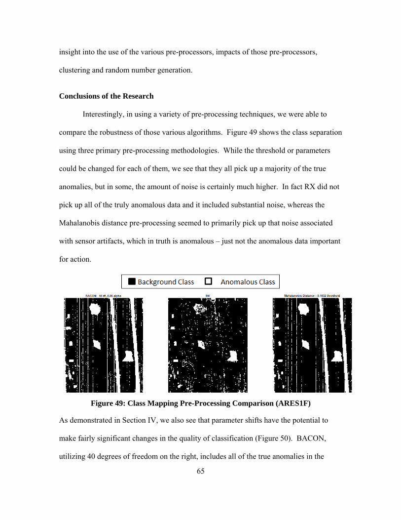
65
insight into the use of the various pre-processors, impacts of those pre-processors,
clustering and random number generation.
Conclusions of the Research
Interestingly, in using a variety of pre-processing techniques, we were able to
compare the robustness of those various algorithms. Figure 49 shows the class separation
using three primary pre-processing methodologies. While the threshold or parameters
could be changed for each of them, we see that they all pick up a majority of the true
anomalies, but in some, the amount of noise is certainly much higher. In fact RX did not
pick up all of the truly anomalous data and it included substantial noise, whereas the
Mahalanobis distance pre-processing seemed to primarily pick up that noise associated
with sensor artifacts, which in truth is anomalous – just not the anomalous data important
for action.
Figure 49: Class Mapping Pre-Processing Comparison (ARES1F)
As demonstrated in Section IV, we also see that parameter shifts have the potential to
make fairly significant changes in the quality of classification (Figure 50). BACON,
utilizing 40 degrees of freedom on the right, includes all of the true anomalies in the
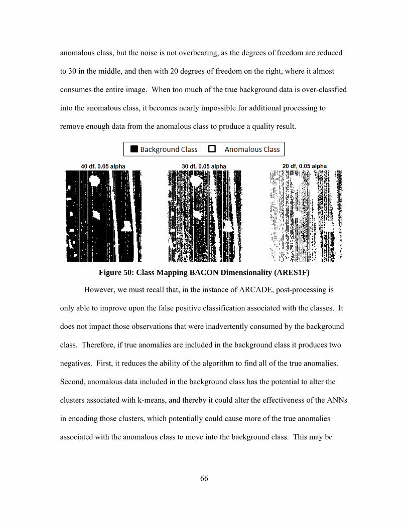
66
anomalous class, but the noise is not overbearing, as the degrees of freedom are reduced
to 30 in the middle, and then with 20 degrees of freedom on the right, where it almost
consumes the entire image. When too much of the true background data is over-classfied
into the anomalous class, it becomes nearly impossible for additional processing to
remove enough data from the anomalous class to produce a quality result.
Figure 50: Class Mapping BACON Dimensionality (ARES1F)
However, we must recall that, in the instance of ARCADE, post-processing is
only able to improve upon the false positive classification associated with the classes. It
does not impact those observations that were inadvertently consumed by the background
class. Therefore, if true anomalies are included in the background class it produces two
negatives. First, it reduces the ability of the algorithm to find all of the true anomalies.
Second, anomalous data included in the background class has the potential to alter the
clusters associated with k-means, and thereby it could alter the effectiveness of the ANNs
in encoding those clusters, which potentially could cause more of the true anomalies
associated with the anomalous class to move into the background class. This may be
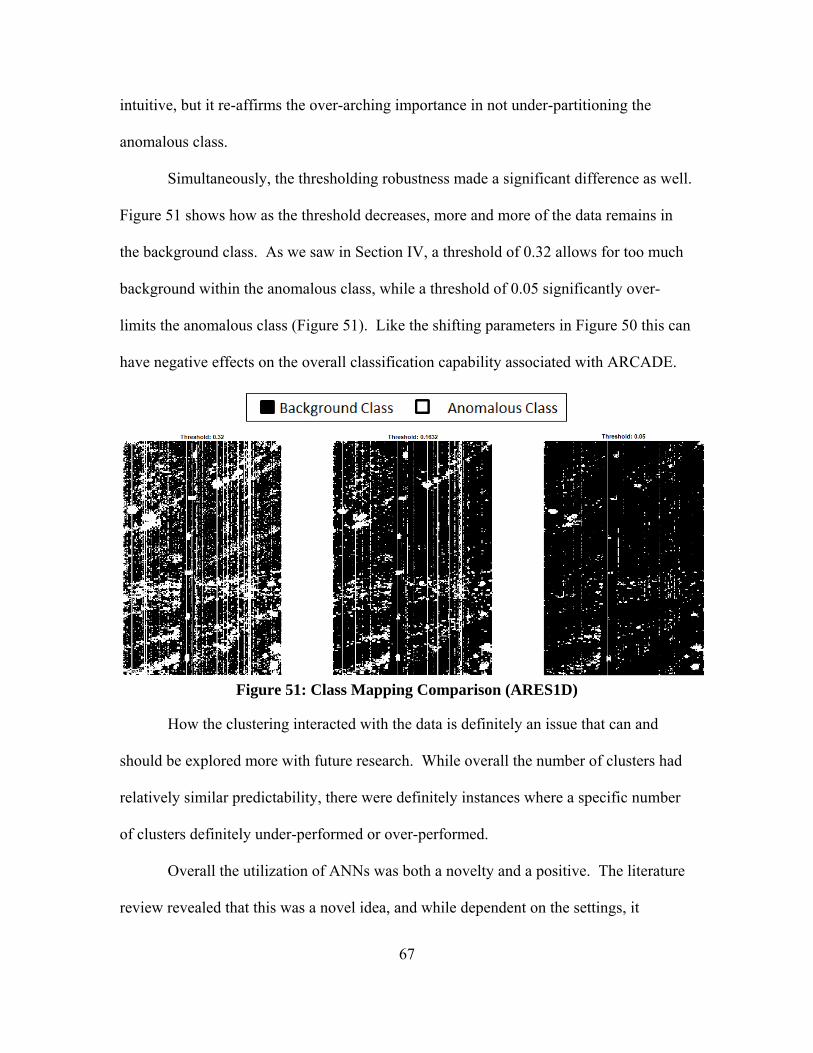
67
intuitive, but it re-affirms the over-arching importance in not under-partitioning the
anomalous class.
Simultaneously, the thresholding robustness made a significant difference as well.
Figure 51 shows how as the threshold decreases, more and more of the data remains in
the background class. As we saw in Section IV, a threshold of 0.32 allows for too much
background within the anomalous class, while a threshold of 0.05 significantly over-
limits the anomalous class (Figure 51). Like the shifting parameters in Figure 50 this can
have negative effects on the overall classification capability associated with ARCADE.
Figure 51: Class Mapping Comparison (ARES1D)
How the clustering interacted with the data is definitely an issue that can and
should be explored more with future research. While overall the number of clusters had
relatively similar predictability, there were definitely instances where a specific number
of clusters definitely under-performed or over-performed.
Overall the utilization of ANNs was both a novelty and a positive. The literature
review revealed that this was a novel idea, and while dependent on the settings, it
68
definitely showed promise in reducing false positives. When examining other research,
we note that other pre-processing algorithms have been shown to hold promise when
compared to both RX and BACON, so additional study in the application of ARCADE in
conjunction with these other algorithms would definitely be worthwhile [16].
Significance of Research
The major additive effects of this research include the noticeable classification
capacity of Mahalanobis distance. With the appropriate thresholding, Mahalanobis
distance is one of the easiest methods for classification, providing high computational
efficiency, while providing a high level of predictability. Using Mahalanobis distance
has been a component of numerous classification techniques [9], but our research
indicates that, at least with the use of HSI images collected with the HYDICE sensor, it
provides a high classification accuracy in and of itself.
Of additional importance, our research shows how the clusters achieve a high
degree of effectiveness with only a relatively small proportion of the associated
observations. When we compared the classification ability utilizing only a 10 percent
sample of each cluster to that of a 40 percent sample, the overall algorithmic performance
was only slightly affected, and not always with an improved result. While computational
efficiency was not the overall goal of this research, this is notable in that the ARCADE
ran fairly quickly despite having literally dozens of moving parts, which could in reality
be scaled down, by slightly tightening the number of clusters or reducing the number of
ANNs run upon each cluster. While current evidence suggests that three ANNs do not
provide enough robustness in performance, 20 ANNs seems to be more than necessary.

69
Of similar importance to the computational efficiency, the 10 percent sample directly
demonstrates the continuity of the clusters, confirming the general quality of k-means
clustering.
Subsequently, this research provided a potentially viable methodology for post-
processing using ARCADE. At minimum, it establishes a starting point into future
research utilizing ANNs in post-processing classification. This combination of
techniques had not been attempted before, but we observed a high level of fidelity when
comparing the potential to other known methods. As ANNs expand in their use and
application, the potential definitely exists to further enhance pattern classification and
anomaly detection.
Lastly, this research firmly asserts that all of these methodologies have potential
in decision-making based upon the goals associated with the analysis. While in a perfect
world, one would classify data and immediately find all of the true positives without
acquiring any false negative observations; this is not typically the case. However, if we
could use these techniques in accordance with our goals, there are many ways which it
could be immediately applicable. In some cases, a few false positives are not very
problematic, but it can have dire consequences not to find all of the anomalies. In other
cases, false positives are absolutely egregious, but if even half of the anomalies could be
resolved, it would create a significant benefit.

70
Recommendations for Action
It would benefit numerous problem sets, especially within the realm of HSI, to
utilize methodological capacities in conjunction with desired intent to either eliminate all
false negatives or enhance the classification of true positives.
Recommendations for Future Research
We would recommend a number of future research options to include:
1) ANN Testing - Testing for the optimal number or range of middle nodes used by the
ANNs - Testing for the optimal number or range of hidden layers in ANNs
2) Signature matching of the anomalous class following completion of ARCADE 3) Testing additional pre-processing methodologies 4) Testing across variations and excursions with Horn’s Curve 5) Further parameter testing for the pre-processing methodologies already tested 6) Optimize sample size 7) Optimize the number of clusters 8) Test various clustering techniques 9) Run replications
Summary
The development of ARCADE provided a first-in-its-class classification
technique utilizing ANNs as a post-processor for data sets that have already been
classified utilizing an already proven pre-processing technique. ARCADE strings
together a variety of mathematical techniques to filter out false positives garnered during
the original classification. While there is still testing to be done, ARCADE shows
promise in this capacity. By developing and testing ARCADE, it provided additional
insight into the robustness of the various classification methods used as a pre-processors,
it gave tremendous insight into the validity and quality of Mahalanobis distance as
classification tool, it demonstrated the robustness of k-means clustering and small sample

71
sizes based on the associated clusters, and it showed promise in the reduction of false
positives. With certainty there is still work to be done, but the information attained will
advance future research possibilities with the possibility of finding ever better anomaly
detection techniques and procedures. Furthermore, this research affirms the necessity in
setting quality goals for anomaly detection. If we can ascertain the intent of our anomaly
detection, we correctly frame problems to have immediate, actionable insights into
varying problem sets.
72
Bibliography
[1] G. R. Hunt, “Spectral Signatures of Particulate Minerals in the Visible and Near Infrared,” Geophysics, vol. 42, no. 3. p. 501, 1977.
[2] F. D. Lee, “The Role of the Terrain Analysis Center (TAC) in Managing the Use of Multispectral Imagery (MSI) for the United States Army.,” Army Engineer Topographic Labs, Fort Belvoir, VA, Tech. Rep. ADA195790, Apr. 21, 1988.
[3] M. B. Satterwhite, “Integrating Multispectral Imagery and Ground Level Hyperspectral Signature Data,” U.S. Army Engineer Topographic Laboratories/Center for Remote Sensing, Research Institute, Fort Belvoir, VA, Tech. Rep. ADA195976, Apr. 8, 1988.
[4] J. N. Rinker, “Hyperspectral Imagery - A New Technique for Targeting and Intelligence,” U.S. Army Topographic Engineering Center, Fort Belvoir, VA, Sci. Paper ADA255406, Jun. 15, 1990.
[5] C.-I. Chang and S.-S. Chiang, “Anomaly detection and classification for hyperspectral imagery,” IEEE Trans. Geosci. Remote Sens., vol. 40, no. 6, pp. 1314–1325, 2002.
[6] D. W. J. Stein, S. G. Beaven, L. E. Hoff, E. M. Winter, A. P. Schaum, and A. D. Stocker, “Anomaly detection from hyperspectral imagery,” IEEE Signal Process. Mag., vol. 19, no. 1, pp. 58–69, 2002.
[7] R. A. Riley, R. K. Newsom, and A. K. Andrews, “Anomaly detection in noisy hyperspectral imagery,” in Proceedings of SPIE, 2004, vol. 5546, pp. 159–170.
[8] J. A. Marin, J. Brockhaus, J. Rolf, J. Shine, J. Schafer, and A. Balthazor, “Assessing band selection and image classification techniques on HYDICE hyperspectral data,” in IEEE International Conference on Systems Man and Cybernetics, 1999, vol. 1, pp. 1067–72 vol.1.
[9] N. Billor, A. S. Hadi, and P. F. Velleman, “BACON: Blocked adaptive computationally efficient outlier nominators,” Comput. Stat. Data Anal., vol. 34, no. 3, pp. 279–298, 2000.
[10] R. J. Johnson, J. P. Williams, and K. W. Bauer, “AutoGAD: An improved ICA-based hyperspectral anomaly detection algorithm,” IEEE Trans. Geosci. Remote Sens., vol. 51, no. 6, pp. 3492–3503, 2013.
[11] K. W. Bauer, S. G. Alsing, and K. A. Greene, “Feature screening using signal-to-noise ratios,” Neurocomputing, vol. 31, no. 1–4, pp. 29–44, 2000.
[12] J. A. East, K. W. Bauer, and J. W. Lanning, “Feature Selection for Predicting Pilot Mental Workload: A Feasibility Study,” International Journal of Smart Engineering System Design, vol. 4, no. 3. pp. 183–193, 2002.
[13] W. R. Dillon and M. Goldstein, Multivariate analysis: methods and applications. Wiley, 1984.
[14] K. Bryan, L. Brennan, and P. Cunningham, “MetaFIND: a feature analysis tool for metabolomics data.,” BMC Bioinformatics, vol. 9, p. 470, 2008.
73
[15] R. M. Haralick, K. Shanmugam, and I. Dinstein, “Textural Features for Image Classification,” IEEE Trans. Syst. Man. Cybern., vol. 3, no. 6, 1973.
[16] T. J. Paciencia, “Improving Non-Linear Approaches to Anomaly Detection, Class Separation, and Visualization,” Ph.D Dissertation, Dept. Operational Sciences, Air Force Institute of Technology, Wright-Patterson AFB, Ohio, 2014.
[17] B. Dean, Thomas (Google Inc.); Wills, Helen (Neuroscience Institute, “Scalable Neuroscience and the Brain Activity Mapping Project,” 2013. [Online]. Available: http://cs.brown.edu/people/tld/note/blog/13/07/26/. [Accessed: 11-Sep-2015].
[18] T. E. Smetek, “Hyperspectral Imagery Target Detection Using Improved Anomaly Detection and Signature Matching Methods,” Ph.D Dissertation, Dept. Operational Sciences, Air Force Institute of Technology, Wright-Patterson AFB, Ohio, 2007.
[19] R. J. Johnson, “Improved Feature Extraction, Feature Selection, and Identification Techniques that Create a Fast Unsupervised Hyperspectral Target Detection Algorithm,” M.S. Thesis, Dept. Operational Sciences, Air Force Institute of Technology, Wright-Patterson AFB, Ohio, 2008.
[20] I. Guyon, I. Guyon, A. Elisseeff, and A. Elisseeff, “An introduction to variable and feature selection,” J. Mach. Learn. Res., vol. 3, pp. 1157–1182, 2003.
[21] J. Fan, R. Samworth, and Y. Wu, “Ultrahigh dimensional feature selection: beyond the linear model.,” J. Mach. Learn. Res., vol. 10, pp. 2013–2038, 2009.
[22] S. Schwartz and K. M. Carpenter, “The right answer for the wrong question: Consequences of type III error for public health research,” Am. J. Public Health, vol. 89, no. 8, pp. 1175–1180, 1999.
[23] V. Chandola, A. Banerjee, and V. Kumar, “Anomaly detection: A survey,” ACM Comput. Surv., vol. 41, no. September, pp. 1–58, 2009.
[24] K. Gao, F. Shao, and R. Sun, “n-INCLOF: A dynamic local outlier detection algorithm for data streams,” Signal Process. Syst., pp. 179–183, 2010.
[25] S. Xiuyao, W. Mingxi, C. Jermaine, S. Ranka, X. Song, M. Wu, C. Jermaine, S. Ranka, S. Xiuyao, W. Mingxi, C. Jermaine, and S. Ranka, “Conditional anomaly detection,” IEEE Trans. Knowl. Data Eng., vol. 19, no. 0325459, pp. 631–644, 2007.
[26] H. Teng, K. Chen, and S. Lu, “Adaptive real-time anomaly detection using inductively generated sequential patterns,” in Research in Security and Privacy, 1990. Proceedings., 1990 IEEE Computer Society Symposium on, 1990, pp. 278–284.
[27] P. J. Rousseeuw and A. M. Leroy, Robust Regression and Outlier Detection, 3rd ed. New York: John Wiley & Sons, Inc., 1987.
[28] J. M. Steppe and K. W. Bauer, “Improved feature screening in feedforward neural networks,” Neurocomputing, vol. 13, no. 1, pp. 47–58, 1996.
[29] L. M. Belue and K. W. Bauer, “Determining input features for multilayer perceptrons,” Neurocomputing, vol. 7, no. 2, pp. 111–121, 1995.
74
[30] J. M. Steppe and K. W. Bauer, “Feature saliency measures,” Computers & Mathematics with Applications, vol. 33, no. 8. pp. 109–126, 1997.
[31] W. A. Young II, T. J. Bihl, and G. R. Weckman, “Artificial Neural Networks for Business Analytics,” in Encyclopedia of Business Analytics and Optimization, 2014, pp. 193–208.
[32] T. L. Fine, Feedforward Neural Network Methodology. Springer Science & Business Media, 2006.
[33] J. J. Hopfield, “Neural networks and physical systems with emergent collective computational abilities.,” Proc. Natl. Acad. Sci. U. S. A., vol. 79, no. 8, pp. 2554–2558, 1982.
[34] J. Deng, Z. Zhang, E. Marchi, and B. Schuller, “Sparse autoencoder-based feature transfer learning for speech emotion recognition,” in Proceedings - 2013 Humaine Association Conference on Affective Computing and Intelligent Interaction, ACII 2013, 2013, pp. 511–516.
[35] A. M. Sarroff and M. Casey, Musical Audio Synthesis Using Autoencoding Neural Nets. Ann Arbor, MI: Michigan Publishing, University of Michigan Library, 2014.
[36] J. Shlens, “A Tutorial on Principal Component Analysis,” Measurement, vol. 51, p. 52, 2005.
[37] K. Fukunaga and W. L. G. Koontz, “Application Of The Karhunen-Loeve Expansion To Feature Selection And Ordering,” Comput. IEEE Trans., vol. C–19, no. 4, pp. 311–318, 1970.
[38] S. Weber, “Bacon: An effective way to detect outliers in multivariate data using Stata (and Mata),” Stata J., vol. 10, no. 3, pp. 331–338, 2010.
[39] B. Du and L. Zhang, “Random-Selection-Based Anomaly Detector for Hyperspectral Imagery,” IEEE Trans. Geosci. Remote Sens., vol. 49, no. 5, pp. 1578–1589, 2011.
[40] L. Dalton, V. Ballarin, and M. Brun, “Clustering algorithms: on learning, validation, performance, and applications to genomics.,” Curr. Genomics, vol. 10, no. 6, pp. 430–445, 2009.
[41] L. H. Chiang, R. J. Pell, and M. B. Seasholtz, “Exploring process data with the use of robust outlier detection algorithms,” J. Process Control, vol. 13, no. 5, pp. 437–449, 2003.
[42] R. F. Caulk, K. B. Reyes, and K. W. Bauer, “Outlier detection in hyperspectral imagery using closest distance to center with ellipsoidal multivariate trimming,” J. Def. Model. Simul. Appl. Methodol. Technol., vol. 9, no. 2, pp. 163–172, 2011.
[43] I. S. Reed and X. Yu, “Adaptive Multiple-Band CFAR Detection of an Optical Pattern with Unknown Spectral Distribution,” IEEE Trans. Acoust., vol. 38, no. 10, pp. 1760–1770, 1990.
[44] M. T. Eismann, “Hyperspectral remote sensing,” 2012. [45] A. Banerjee, P. Burlina, and R. Meth, “Fast hyperspectral anomaly detection via
75
SVDD,” in Proceedings - International Conference on Image Processing, ICIP, 2006, vol. 4.
[46] J. A. Jablonski, T. J. Bihl, and K. W. Bauer, “Principal Component Reconstruction Error for Hyperspectral Anomaly Detection,” IEEE Geosci. Remote Sens. Lett., vol. 12, no. 8, pp. 1725–1729, 2015.
[47] J. Macqueen, “Some methods for classification and analysis of multivariate observations,” Proc. Fifth Berkeley Symp. Math. Stat. Probab., vol. 1, pp. 281–297, 1967.
[48] R. Gelbard, O. Goldman, and I. Spiegler, “Investigating diversity of clustering methods: An empirical comparison,” Data Knowl. Eng., vol. 63, pp. 155–166, 2007.
[49] “k-means clustering - MATLAB kmeans.” [Online]. Available: http://www.mathworks.com/help/stats/kmeans.html?s_tid=gn_loc_drop#buefthh-3. [Accessed: 31-Dec-2015].
[50] J. A. Jablonski, “Reconstruction Error and Principal Compenent Based Anomaly Detection in Hyperspectral Imagery,” M.S. Thesis, Dept. Operational Sciences, Air Force Institute of Technology, 2014.
76
REPORT DOCUMENTATION PAGEForm Approved OMB No. 074-0188
The public reporting burden for this collection of information is estimated to average 1 hour per response, including the time for reviewing instructions, searching existing data sources, gathering and maintaining the data needed, and completing and reviewing the collection of information. Send comments regarding this burden estimate or any other aspect of the collection of information, including suggestions for reducing this burden to Department of Defense, Washington Headquarters Services, Directorate for Information Operations and Reports (0704-0188), 1215 Jefferson Davis Highway, Suite 1204, Arlington, VA 22202-4302. Respondents should be aware that notwithstanding any other provision of law, no person shall be subject to an penalty for failing to comply with a collection of information if it does not display a currently valid OMB control number. PLEASE DO NOT RETURN YOUR FORM TO THE ABOVE ADDRESS. 1. REPORT DATE (DD-MM-YYYY)
24-03-2016 2. REPORT TYPE
Master’s Thesis 3. DATES COVERED (From – To)
Sep 14 – Mar 16
TITLE AND SUBTITLE
Autoencoded Reduced Clusters for Anomaly Detection Enrichment (Arcade) In Hyperspectral Imagery
5a. CONTRACT NUMBER
5b. GRANT NUMBER
5c. PROGRAM ELEMENT NUMBER
6. AUTHOR(S)
McLean, Brenden A., Captain, USAF
5d. PROJECT NUMBER
5e. TASK NUMBER
5f. WORK UNIT NUMBER
7. PERFORMING ORGANIZATION NAMES(S) AND ADDRESS(S) Air Force Institute of Technology Graduate School of Engineering and Management (AFIT/EN) 2950 Hobson Way, Building 640 WPAFB OH 45433-8865
8. PERFORMING ORGANIZATION REPORT NUMBER
AFIT-ENS-MS-16-M-119
9. SPONSORING/MONITORING AGENCY NAME(S) AND ADDRESS(ES) AF/A9FC 1570 Air Force Pentagon, Washington D.C. 20330-1570 PHONE and EMAIL: (571) 256-2147/[email protected] ATTN: Major Todd J. Paciencia
10. SPONSOR/MONITOR’S ACRONYM(S) AF/A9FC
11. SPONSOR/MONITOR’S REPORT NUMBER(S)
12. DISTRIBUTION/AVAILABILITY STATEMENT DISTRUBTION STATEMENT A. APPROVED FOR PUBLIC RELEASE; DISTRIBUTION UNLIMITED.
13. SUPPLEMENTARY NOTES This material is declared a work of the U.S. Government and is not subject to copyright protection in the United States. 14. ABSTRACT Anomaly detection in hyper-spectral imagery is a relatively recent and important research area. The shear amount of data available in a many hyper-spectral images makes the utilization of multivariate statistical methods and artificial neural networks ideal for this analysis. Using HYDICE sensor hyper-spectral images, we examine a variety of pre-processing techniques within a framework that allows for changing parameter settings and varying the methodological order of operations in order to enhance detection of anomalies within image data. By examining a variety of different options, we are able to gain significant insight into what makes anomaly detection viable for these images, as well as what impact parameter and methodology changes can have on the total classification effectiveness, false positive fraction and true positive fraction regarding classification.
15. SUBJECT TERMS Anomaly Detection, Clustering, Reconstructive Error, Mahalanobis Distance
16. SECURITY CLASSIFICATION OF:
17. LIMITATION OF ABSTRACT
UU
18. NUMBER OF PAGES
89
19a. NAME OF RESPONSIBLE PERSON Dr. Kenneth W. Bauer Jr., AFIT/ENS
a. REPORT
U
b. ABSTRACT
U
c. THIS PAGE
U
19b. TELEPHONE NUMBER (Include area code) (937) 255-3636, ext 4328 (NOT DSN) ([email protected])
Standard Form 298 (Rev. 8-98) Prescribed by ANSI Std. Z39-18