aid under fire: development projects and civil con ictneudc2012/docs/paper_268.pdf · aid under...

Aid Under Fire: Development Projects andCivil Conflict∗

Benjamin CrostUniversity of Colorado Denver

Joseph FelterStanford University

Patrick JohnstonRAND Corporation

October 9, 2012

Abstract

We estimate the causal effect of a large development program on conflict in thePhilippines through a regression discontinuity design that exploits an arbitrary povertythreshold used to assign eligibility for the program. We find that barely eligible munic-ipalities experienced a large increase in conflict casualties compared to barely ineligibleones. This increase is caused by insurgent-initiated incidents during the early stagesof program-preparation. Our results are consistent with two mechanisms: that insur-gents attempt to appropriate the program’s resources by violent means or that theytry to sabotage the program because its success would weaken their support in thepopulation.

∗The authors would like to thank Eli Berman, Michael Callen, Alexander B. Downes, Alain de Janvry,Jim Fearon, Julien Labonne, David D. Laitin, Ethan Ligon, Jeremy Magruder, Ted Miguel, Andrew Parker,Bob Powell, Elisabeth Sadoulet, Jacob N. Shapiro, Rob Wrobel, and participants of the NBER SummerInstitute on the Economics of National Security for comments on earlier versions of the manuscript. Crostacknowledges financial support from the Institute of Business and Economic Research and the Center ofEvaluation for Global Action at the University of California, Berkeley. Felter and Johnston acknowledgefinancial support from AFOSR Award #FA9550-09-1-0314. Any opinions, findings, conclusions, and recom-mendations expressed in this publication are the authors’ and do not necessarily reflect those of any otherorganization or entity.

1 Introduction

Governments and international donors target large amounts of development aid to conflict-

affected areas throughout the world. Despite this significant influx of resources, it remains

unclear how aid affects conflict. The evidence is varied. Using fixed-effects approaches,

Berman et al. (2011) and Iyengar et al. (2011) show that increases in spending on (labor-

intensive) reconstruction programs led to reductions in insurgent attacks in Iraq. Beath

et al. (2011) present experimental evidence that aid has increased popular support for the

government in Afghanistan, but no evidence that this has led to a decrease in insurgent

attacks there. Indirect evidence for a possible positive effect of aid comes from Miguel et

al. (2004) and Dube and Vargas (2011), who find that economic shocks - in the form of

good rainfall and favorable world market prices for agricultural goods - caused a decrease

in conflict in Africa and Colombia, respectively. On the other hand, Nunn and Qian (2012)

find that U.S. food aid causes an increase in conflict in recipient countries.

This article enhances our understanding of the effect of development aid on conflict by esti-

mating the causal effect of a large development program - the Philippines’ Kapit-Bisig Laban

sa Kahiripan - Comprehensive Integrated Delivery of Social Services (KALAHI-CIDSS) - on

casualties in armed civil conflict. Financed by the World Bank with a budget of $180 million,

KALAHI-CIDSS was the Philippines’ flagship anti-poverty program from 2003 through 2008.

KALAHI-CIDSS is a community-driven development (CDD) program, a common type of de-

velopment intervention and an increasingly popular tool for delivering aid in conflict-affected

countries (Mansuri and Rao, 2004). Our empirical strategy is a regression discontinuity (RD)

design, that exploits an arbitrary eligibility threshold for the program that restricted eligi-

bility to the poorest 25 percent of municipalities in participating Philippine provinces. This

eligibility threshold created a discontinuity in aid assignment, which allows us to identify its

causal effect by comparing municipalities just above and just below the threshold. Our em-

pirical strategy allows us to overcome the problem of endogenous aid allocation and cleanly

identify the causal effect of aid on conflict casualties. Data on this outcome were com-

piled from comprehensive information on conflict incidents involving the Armed Forces of

the Philippines (AFP) between 2002 and 2009. The data were derived from the text of the

AFP’s original incident reports. It is similar to the US military’s “Significant Activities”

(SIGACTS) data, which has been used to advance the study of conflict based on the US

experiences in Afghanistan and Iraq (Berman et al., 2011; Iyengar et al., 2011; Beath et al.,

2011).

In contrast to much of the previous literature, we find that aid exacerbated violent conflict in

this context. For the duration of this community-driven development program, municipalities

that were barely eligible for the program suffered a large and statistically significant increase

in violence compared to municipalities that were barely ineligible. We find no differences in

pre- and post-program violence or other observable characteristics that could explain this

effect. Further results show that most of the excess casualties occurred in the early stages of

program preparation, in insurgent-initiated incidents, and that the bulk of casualties were

suffered by government forces.

Our results are consistent with at least two possible mechanisms through which aid could

increase conflict. The first is that an influx of aid will increase the amount of resources to

be fought over, which in turn increases the incentive to fight. This mechanism has been de-

scribed in a number of theoretical models (e.g. Hirshleifer, 1989; Grossman, 1991; Skaperdas,

1992; Dal Bo and Dal Bo, 2011). The second is that aid increases short-term conflict be-

cause it has the potential to weaken insurgents in the long-run, perhaps because it increases

peaceful economic opportunities or popular support for the government. If insurgents ex-

pect a succesful aid program to weaken their position, they have an incentive to sabotage its

implementation by violent means.1 We discuss the consistency of our evidence with these

two mechanisms in Section 4.

1See Powell (2012) for a detailed theoretical account of how expected future shifts in power can lead toconflict.

2

1.1 Institutional Background: The KALAHI-CIDSS Program

This paper studies the KALAHI-CIDSS program; a CDD program implemented by the

Philippine government’s Department of Social Welfare and Development and funded through

World Bank loans. The program aims to enhance local infrastructure, governance, partici-

pation, and social cohesion. As of mid-2009, the end of our study period, more than 4000

villages in 184 municipalities across 40 provinces had received aid through KALAHI-CIDSS,

making it the largest development program in the country during this period.2 Plans are

currently being made to expand KALAHI-CIDSS, with the aim of doubling the number

of recipient municipalities during the program’s next phase. Figure 1 shows a map of the

municipalities that received KALAHI-CIDSS aid during our period of observation.

Community-driven development programs are a common type of development intervention

that has become a popular tool for delivering aid in conflict-affected countries. The World

Bank lends more than two billion dollars annually for CDD projects (Mansuri and Rao 2004).

Over the last decade, for example, CDD programs have been implemented in Afghanistan,

Angola, Colombia, Indonesia, Nepal, Rwanda, and Sudan. KALAHI-CIDSS follows a stan-

dard CDD template. In the six months before the program begins, inhabitants of eligible

municipalities are informed of the project and its procedures in a so-called “social prepara-

tion phase.” Once the program officially begins, the participating municipalities receive a

block grant for small-scale infrastructure projects. Each village within participating munici-

palities holds a series of meetings in which village members draft project proposals. Villages

then send democratically elected representatives to participate in municipal-level inter-village

fora, in which proposals are evaluated and funding is allocated. Proposals are funded until

each municipality’s grant has been exhausted. Once municipality funding has been allocated,

community members are encouraged to monitor or participate in project implementation.3

2As of March 2010, there were 80 provinces and 1496 municipalities in the Philippines.3See Parker (2005) for a detailed overview of the KALAHI-CIDSS process.

3

The amount of aid distributed through KALAHI-CIDSS is substantial. Participating mu-

nicipalities receive PhP300,000, or approximately $6000, per village in their municipality.

The average municipality has approximately 25 villages, making the average grant approxi-

mately $150,000, or about 15% of an average municipality’s annual budget. Over the course

of the program, the project cycle is repeated three times–occasionally four–meaning that

on average, participating municipalities receive a total of between $450,000 and $600,000

dollars.

2 Empirical Strategy

To estimate the causal effect of KALAHI-CIDSS on the intensity of violent conflict, we use

a regression discontinuity (RD) design. The RD design is made possible by an arbitrary

eligibility threshold that was used to target the program. Targeting followed a two-staged

approach. First, 42 eligible provinces were selected, among them were the 40 poorest in the

country based on estimates from the Family Income and Expenditure Survey (FIES). The

poverty levels of all municipalities within the eligible provinces were estimated using a poverty

mapping methodology based on a combination of data from FIES and the 2000 Census of

the Philippines (Balisacan et al., 2002; Balisacan and Edillon, 2003). The estimation was

carried out by an independent consulting firm in order to make sure that it was based on

objective criteria. In each eligible province, municipalities were ranked according to their

poverty level and only the poorest quartile was eligible for KALAHI-CIDSS.

Each municipality’s poverty score was calculated as a weighted combination of variables from

the 2000 census and variables from a database on road conditions from the Department of

Transportation. The road database is no longer available, so we are unable to replicate the

raw poverty scores and use them as the running variable of our RD design. Instead, we

directly use the rankings published by Balisacan et al. (2002) and Balisacan and Edillon

4

(2003) to generate the running variable, which is the distance of the municipality’s poverty

rank from the provincial eligibility threshold. Since only municipalities in the poorest quartile

were eligible, the provincial threshold was calculated by dividing the number of municipalities

in each province by four and then rounding to the nearest integer.4 This threshold number

was then subtracted from the municipality’s actual poverty rank to obtain its relative poverty

rank. For each participating province, the richest eligible municipality has a relative poverty

rank of zero and the poorest ineligible municipality has a relative poverty rank of one.

Since the poverty ranking was used exclusively to target KALAHI-CIDSS and no other

program, the only variable that should change discontinuously at this threshold is eligibility

for KALAHI-CIDSS.

Our goal is to estimate the discontinuous change in conflict casualties across the eligibility

threshold. Assuming that the unobserved variables are a smooth function of the running

variable, this change reflects the causal effect of the KALAHI-CIDSS program. To ensure

that our results are robust to different assumptions about the shape of this smooth function,

we follow Ludwig and Miller (2007) and use two different specifications to obtain the RD

estimator of the program’s effect. The first is a regression that flexibly controls for quadratic

trends on both sides of the threshold:

Yit = β0 + τDi + β1Xi + β2X2i + β3DiXi + β4DiX

2i + αt + εit

Yit denotes the number of conflict casualties suffered by municipality i in month t. Xi

denotes the municipality’s relative poverty rank. Di is an indicator that takes the value 1 if

the municipality is eligible for the program and 0 if it is not. The RD estimator is given by

the parameter τ .

4In cases where dividing a province’s number of municipalities by 4 ended on .5, the number of eligiblemunicipalities was rounded down more often than up. We follow this approach and round down at .5, whichimproves the accuracy with which the relative poverty rank predicts participation in the program.

5

The second specification is a nonparametric local linear regression. This approach estimates

the following linear regression, while using kernel weights to give higher weight to observa-

tions that are closer to the threshold:

Yit = β0 + τDi + β1Xi + β2DiXi + αt + εit

Our baseline specification uses a triangular kernel with a bandwidth of 6 poverty ranks. Since

there is currently no universally agreed-upon method for selecting the optimal bandwidth for

local linear regressions, we follow Ludwig and Miller (2007) and also report results for a wide

range of bandwidths between 1 and 6 ranks. The unit of observation is the municipality-

month. Since our outcome of interest is a discrete “count” variable, we estimate both OLS

and Poisson models. To deal with the potential serial and spatial correlation of conflict in

our sample, the standard errors of all specifications are clustered at the province level.

When interpreting the results of this approach, it should be kept in mind that not all eligible

municipalities participated in the program. Some municipalities declined to participate,

and several others were dropped from the program by the implementing agency due to

concerns about the security of its staff. Our results therefore constitute an “intention-to-

treat” effect - the effect of eligibility for the program regardless of later participation status.

One might think that it would be preferable to estimate the local average treatment effect

of program participation by “fuzzy” RD design that uses eligibility as an instrument for

participation. However, we show in section 4 that a large part of the increase in violence

occurred during the program’s social preparation phase, which took place in all eligible

municipalities, before it was clear whether they would actually participate in the program.

Thus it appears that in many cases eligibility alone was sufficient to cause an increase in

6

violence even in municipalities that did not ultimately participate in the program.5 This

violates the exclusion restriction of the IV estimator; as a consequence, we only estimate the

intention-to-treat effect.

2.1 Timing of the Program

Our goal is to estimate the effect of the KALAHI-CIDSS program on conflict during the

period when the program was active as well as the pre-program and post-program periods. As

mentioned in section 1.1, the first program activity was the social preparation phase, which

took place in all eligible municipalities and began 6 months before the program was scheduled

to start in participating municipalities. Overall, the scheduled duration of program activities

was 3 years. We therefore define the program-period (including the social preparation phase)

as lasting from 6 months before until 30 months after the program’s scheduled start date.6

Our analysis is complicated somewhat by the fact that the program’s implementing agency,

DSWD, had a certain amount of leeway when choosing the program’s start date in a mu-

nicipality. This raises the concern that our results may be biased due to endogenous timing

of the program. It is possible, for example, that DSWD scheduled eligible municipalities

to receive the program at times when they were expected to have more (or less) conflict

than usual. As a result, eligible municipalities would have more (or less) conflict during the

program period than ineligible ones, even if the program had no effect on conflict. In order

to ensure that this does not affect our results, our analysis only makes use of decisions about

the start date that were made at the province level, before the municipality-level poverty

rankings were calculated. At that time, DSWD did not yet know which municipalities would

5Anecdotal evidence suggests that some insurgent groups used violence to intimidate the population andkeep the municipality from participating in the program (personal interview with DSWD director and seniorproject managers).

6We also separately estimate the program’s effect during the social preparation phase and during theremaining program period.

7

be eligible, so it could not have manipulated the program’s schedule based on unobserved

characteristics of eligible municipalities.7

To describe our empirical approach, it is necessary to review the program’s timeline in some

detail. KALAHI-CIDSS was rolled out in 5 phases, the start dates of which are shown in

Table 1. The phases did not differ in any way except for their start dates. The assignment

of municipalities to phases was made in two steps. In 2002 - before the poverty ranking was

calculated - the participating provinces were divided into two groups, which we call Batch A

and Batch B. All municipalities in Batch A provinces were covered in Phase 2 of the program,

whose scheduled start date was June 2003.8 Since provinces were assigned to batches before

eligibility was determined, endogenous timing is not an issue for municipalities in Batch A.

Municipalities in Batch B provinces were covered in Phases 3A, 3B and 4. Municipalities

in Batch B were assigned to phases after eligibility was determined. Thus, endogenous

timing is a potential problem, since DSWD might have assigned municipalities to phases

based on unobserved information about how much conflict they would experience at a given

time. To address this concern, we define the program’s start date for all municipalities in

Batch B provinces to be the start date of the largest of the three phases, Phase 4, which

began in August 2006. This approach ensures that the start date used in our analysis only

depends on the assignment of provinces to batches, which was determined before DSWD

knew which municipalities would be eligible. Thus, eligible and ineligible municipalities

should not differ in unobserved characteristics at the start date. By assigning the same start

date to all municipalities in the same province, our estimator is based on comparing eligible

and ineligible municipalities in the same province during the same time period. To make

sure that our results are not driven by the way we deal with endogenous timing, we conduct

two robustness tests, the results of which are reported in the appendix. First, we present

7The poverty ranking was calculated by an independent consulting firm so that DSWD did not know inadvance which municipalities would be eligible for the program.

8Phase 1 was a pilot phase, for which municipalities were chosen independently of the poverty ranking,so that it is not relevant for our analysis.

8

estimates based only on the subsample of municipalities in Batch A provinces, for which

endogenous timing is not an issue. Second, we implement an alternative method for choosing

the start date for Batch B, in which we weight observations by the ex-ante probability with

which municipalities were covered by the program at the time of the observation.9

2.2 Robustness Tests

We conduct several robustness tests to evaluate the validity of the RD estimator. The first

concern is that DSWD manipulated the poverty ranking, to target the program towards

certain municipalities. As a test for this, we estimate whether eligible and ineligible mu-

nicipalities differed in observable characteristics before the start of the program. If the

assumptions of the RD estimator hold, we should not observe a systematic change in observ-

able (and unobservable) pre-program characteristics at the eligibility threshold. In addition,

the appendix reports placebo tests for discontinuities in post-treatment variables that are

unlikely to have been affected by the program. A second concern is that DSWD had advance

knowledge of the outcome of the poverty ranking and used this knowledge to manipulate the

timing of the program. As a robustness test for this, we estimate the program’s “effect” on

conflict in the 12 months leading up to the start of the social preparation phase. If DSWD

had manipulated start dates in order to target the program to municipalities with more (or

less) conflict, we would expect eligible and ineligible municipalities to have systematically

different levels of conflict even before the program began. The results of both of these tests

are reported in Section 4. As a third robustness test, we examine whether there are dis-

continuities in conflict at other “pseudo-thresholds” where eligibility for the program did

9Out of the 117 municipalities that were covered in Batch B, 34 were covered in Phase 3A, 29 in Phase3B and the remaining 54 in Phase 4. We therefore assigned a weight of 34

117 to municipalities during theprogram period of Phase 3A, which started in October 2004, a weight of 29

117 to observations during theperiod of Phase, which started in January 2006, and a weight of 54

117 to observations in the program periodof Phase 4, which started in August 2006. Observations outside of the program period of any phase receive aweight of zero. For observations that fall into the program period of several phases the weights were assignedadditively. For example, observations in March 2006, when Phases 3A and 3B were both active, receive aweight of 34+29

117 . The results of this test are reported in the appendix.

9

not change, which might occur if our results were due to mis-specification of the relation-

ship between running variable and outcome. The results of these tests are reported in the

appendix.10

3 Data

The data on civil conflict and violence used in this paper come from the Armed Forces of the

Philippines’ (AFP) records of civil conflict-related incidents. The data were derived from

the original incident reports of AFP units operating throughout the Philippines from 2002

through 2009. The incident-level data are similar to the US military’s SIGACTS data, which

have been used to study the conflicts in Afghanistan and Iraq (Berman et al., 2011; Iyengar

et al., 2011; Beath et al., 2011). The dataset contains information on the date, location, the

insurgent group involved, the initiating party, and the total number of casualties suffered by

government troops, insurgents, and civilians (see Felter 2005). The data are comprehensive,

covering every conflict-related incident reported to the AFP’s Joint Operations Center (JOC)

by units deployed across the country. In total, the database documents more than 21,000

unique incidents during this period, which led to just under 10,000 casualties. The depth,

breadth, and overall quality of the AFP’s database makes it a unique resource for conflict

researchers.

One concern about the data is that AFP troops may selectively report the number of casu-

alties that they experience. While this should be kept in mind when interpreting the results,

we believe that the extent of misreporting is limited. First, the original field reports our data

is coded from are for internal use by the Armed Forces of the Philippines and the AFP’s

10One disadvantage of our design is that we cannot use the density of the running variable to test forpossible manipulations of the poverty ranking. Since there are as many municipalities that are one rankbelow the eligibility cutoff as there are one rank above it, the density of the running variable is smooth byconstruction. It is therefore impossible to detect manipulations by testing for “bunching” of municipalitiesat the threshold.

10

chain of command has a strong incentive to enforce accurate reporting. The reports sent

to the JOC are collected in part to develop intelligence assessments and plan future AFP

operations. Inaccurate information included in field reports might jeopardize future military

operations and put the lives of AFP troops at risk. Concerns about misreporting should be

further limited by the fact that we focus on casualties as the outcome of interest.11 Casualties

are relatively easy to verify, which limits the likelihood that AFP units misreport casualties,

even if they had an incentive to do so.12 Moreover, tests reported in section 4 indicate that

our results are largely driven by an increase in government casualties, which are the easiest

outcome to verify by the JOC. The information on which party initiated the incident, which

we use to distinguish between government-initiated and insurgent-initiated violence can in

some cases be subjectively interpreted and is more likely to be prone to misreporting. How-

ever, previous studies make similar distinctions based on comparable data reported by US

military units in the SIGACTS data (e.g. Berman et al., 2011; Iyengar et al., 2011; Beath et

al., 2011) and we follow this approach to ensure that our results are comparable with those

of the literature.

The second concern is that eligible municipalities may experience more casualties simply

because more AFP troops are present to engage in conflict with insurgents. It is, for example,

possible that the AFP moved its troops towards eligible municipalities to enhance the security

of the program. If this was the case, the program may not have increased aggregate conflict

in the country as a whole, but merely shifted it from one location to another by acting as

a “conflict magnet.” To address this concern, we estimate the program’s spillover effect on

conflict in nearby municipalities. If the program’s effect was mainly due to troop movements,

11We find the same qualitative results when using raw incident counts as the outcome of interest, thoughthe point estimates are slightly smaller and less precisely estimated.

12Note, however, that using data from newspaper reports, Arcand et al. (2010) find that the KALAHI-CIDSS program caused a decrease in casualties, at least for one of the conflicts in the Philippines. However,their data contains a much smaller number of incidents and likely has more missing data than ours. Forexample, they report an average of only 0.42 incidents per year within a 100km radius around each mu-nicipality (given the dense population of the Philippines, a 100km radius contains on average over 35 othermunicipalities). The precision of our data allows us to more accurately map casualties to municipalities.

11

we would expect conflict to decrease in the municipalities that the troops were moved from,

which are likely to be nearby. The results of this analysis are presented in Section 4.9 and

show no evidence of a spillover effect.

4 Results

4.1 Summary Statistics

Table 2 reports summary statistics of conflict outcomes and control variables in our sample

of municipalities within 6 ranks of the eligibility threshold for the KALAHI-CIDSS program.

The statistics show that the conflict is of relatively low-intensity, with approximately 0.078

casualties per municipality per month, or 0.94 casualties per municipality per year. The

majority of the casualties are suffered by government forces and occur as a result of incidents

initiated by insurgents. Out of the three main insurgent groups, incidents involving the

communist New People’s Army (NPA) account for the vast majority of casualties. The

conflict with the Muslim-separatist Moro-Islamic Liberation Front (MILF) has a smaller

geographic reach (the MILF is only active in parts of the southern island of Mindanao

and the Sulu Sea), and therefore accounts for a smaller fraction of total casualties. The

third group, referred to in the AFP data as “Lawless Elements”, is comprised by organized

criminal groups without clearly defined political goals. These groups also account for only

a small fraction of total casualties. As expected, based on the program’s eligibility criteria,

the summary statistics of the control variables show that municipalities in the sample are

relatively poor. For example, in the average municipality less than 40% of households have

access to electricity and only approximately 50% have access to indoor plumbing.

12

4.2 Eligibility and Participation

Figure 2 plots the observed probability of participating in KALAHI-CIDSS against the rel-

ative poverty rank. As in all of the graphs that follow, the scatter dots represent average

values for bins with a width of 2 poverty ranks. The vertical bars are 95% confidence inter-

vals. The size of the scatter dot represents the number of municipalities within the bin. The

dashed line represents a quadratic fit to the data and the solid line presents a local linear fit

with a triangular kernel and a bandwidth of 6. The graph shows that the probability of par-

ticipation decreases sharply at the eligibility threshold, though some eligible municipalities

did not participate and were replaced by municipalities above the threshold. As discussed

in section 2, participation in the program is potentially endogenous to the conflict, since

several municipalities did not participate due to security concerns. Our empirical analysis

therefore estimates the “intention to treat” effect - the effect of eligibility regardless of later

participation status. Table 3 shows the results of RD regressions of the effect of eligibility on

participation. The results show that the probability of participation increased significantly

at the eligibility threshold, by between 28 and 47 percentage points.

4.3 The Effect of KALAHI-CIDSS on Conflict Casualties

Figure 3 graphically displays the relationship between conflict casualties and the relative

poverty rank. The top left panel shows the relationship for the entire duration of the program.

The graph shows that barely eligible municipalities - the ones whose poverty ranks put them

just below the eligibility threshold - suffered more total casualties than barely ineligible

municipalities, which suggests that the program had a causal effect on casualties. The

graph also shows that for eligible municipalities, casualties decreased with distance to the

threshold. This raises the possibility that the program’s effect may not be the same for

all eligible municipalities. A look at the graphs of control variables in Figure 4 shows that

13

municipalities further away from the threshold have smaller populations, less highway access,

and are less fractionalized ethnically and religiously. Possible explanations for the trend are

therefore that the program’s effect is proportional to population and/or that the program

only increases conflict in fractionalized municipalities, where there is a higher potential for

disagreement (of course it is also possible that municipalities further from the threshold differ

in unobserved variables that explain the trend).

Panel A of Table 4 presents the corresponding regression results from the estimating equa-

tions in Section 2. The table shows that the program has a significant positive (in sign) effect

on total casualties during the 3 years after the program’s start. Depending on the specifica-

tion, the effect size ranges between 0.071 and 0.11 casualties per month, which corresponds

to between 0.95 and 1.32 casualties per year. This effect is large relative to the average level

of conflict casualties in the sample of approximately 0.078 per month or 0.94 per year. If

we assumed the effect was constant across all 184 municipalities that received the program,

the program would have caused between 470 and 720 excess casualties during the 3 years in

which it was active.

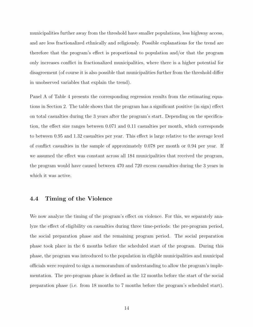
4.4 Timing of the Violence

We now analyze the timing of the program’s effect on violence. For this, we separately ana-

lyze the effect of eligibility on casualties during three time-periods: the pre-program period,

the social preparation phase and the remaining program period. The social preparation

phase took place in the 6 months before the scheduled start of the program. During this

phase, the program was introduced to the population in eligible municipalities and municipal

officials were required to sign a memorandum of understanding to allow the program’s imple-

mentation. The pre-program phase is defined as the 12 months before the start of the social

preparation phase (i.e. from 18 months to 7 months before the program’s scheduled start).

14

The remaining program period is defined as the 30 months after the program’s scheduled

start.

The results in Figure 3 and Table 4 show that the program’s effect is concentrated in the

social preparation phase. During this period, eligible municipalities experienced between 0.25

and 0.39 excess casualties per month. By contrast, the program’s estimated effect during

the remaining program period was between 5 and 10 times smaller and not statistically

significant in most specifications. These findings are consistent with the hypothesis that

insurgents attacked eligible municipalities in order to sabotage the program. This would

have been easiest during the social preparation phase, when municipalities had not yet

decided whether to actually participate in the program (in fact, several municipalities opted

out or were dropped from the program at this stage by DSWD due to concerns about the

security situation). The findings are perhaps less easy to explain with the hypothesis that

insurgents tried to appropriate the program’s resources, since funds were not disbursed until

the beginning of the program. However, it is possible that insurgents tried to extort payments

from municipal officials in return for allowing the program proceed, and launched attacks

during the social preparation phase in order to make their threats credible, so a variant of

this mechanism cannot be ruled out.

The estimates of the program’s “effect” during the pre-program phase serve as a robustness

tests for possible violations of the RD assumptions. Here, the concern is that the poverty

ranking or the timing of the rollout was manipulated in order to give the program to mu-

nicipalities that were more (or less) heavily affected by conflict. If this were the case, we

would expect eligible municipalities to have significantly more (or fewer) casualties even

before the program becomes active. The results in Panel B of Table 4 show no evidence

of this. Barely eligible and barely ineligible municipalities experienced almost exactly the

same number of casualties in the pre-program period and the difference is not statistically

15

significant. This increases our confidence that the poverty ranking was not manipulated and

that the assumptions of the RD estimator hold.

4.5 Balance Tests

Table 5 shows the results of a series of robustness tests for smoothness of pre-treatment

observable variables across the threshold. These tests estimate the same equations used to

estimate the program’s effect on casualties, but use a number of control variables as the de-

pendent variable. The parameter associated with eligibility reflects the discontinuous change

in the control variables across the eligibility threshold. Under the identifying assumption of

the RD estimator - that assignment close to the threshold is as good as random - the control

variables should not change systematically across the threshold. The results in Figure 4 and

Table 5 are consistent with this assumption. The “effect” of eligibility is not statistically

significant for any of the control variables, which suggests that the variables did not differ

systematically across the eligibility threshold.13

4.6 Robustness to Choice of Bandwidth

As mentioned in Section 2, there is currently no widely agreed-upon method for selecting the

optimal bandwidth for local linear regressions. We therefore follow Ludwig and Miller (2007)

and report results for a wide range of bandwidths. Table 6 shows that the estimates of the

program’s effect on total casualties in the entire program period and the social preparation

13We conducted two additional robustness tests and report their results in the appendix. First, we esti-mated the change across the threshold in an outcome that we do not expect to be affected by the program- the 2003 poverty rate - and found no evidence of a discontinuity. Second, we tested for discontinuitiesin casualties at values of the running variable away from the threshold. Finding discontinuities at those“pseudo-thresholds”, where eligibility does not change, would raise the concern that our results are dueto mis-specified non-linearities in the relationship between the running variable and the outcome Imbensand Lemieux (2008). Following Imbens and Lemieux’s recommendation, we tested for discontinuities at themedians of the running variable for eligible and ineligible municipalities, located at -2 and 3 relative povertyranks, respectively. We found no evidence for a statistically significant change in the outcome across thesethresholds. These results are reported in the Appendix.

16

phase is positive and statistically significant (at least at the 10% level) for all bandwidths

between 1 and 6 ranks.14 The estimates for the entire program period range between 0.07

and 0.10, while the estimates for the social preparation phase range between 0.27 and 0.50.

The estimated effect on casualties in the pre-program phase and the remaining program

phase (not including the social preparation phase) are not statistically significant for any of

the bandwidths. Overall, the robustness test increases our confidence that our results are

not dependent on the choice of a particular bandwidth for the RD design.

4.7 Who Suffers the Casualties?

The top two panels in Figure 5 suggest that the discontinuous change across the eligibility

threshold is particularly strong for casualties in insurgent-initiated incidents, and much less

pronounced for casualties in government-initiated incidents. The corresponding results in

Table 7 supports this conclusion. The program’s effect is mainly due to its effect on casual-

ties in insurgent-initiated incidents, which ranges between 0.050 and 0.086 and is statistically

significant in all specifications. The program’s estimated effect on casualties in government-

initiated incidents is between 3 and 5 times smaller and not statistically significant in any

of the specifications. This result is consistent with the hypothesis that the program in-

creased the insurgents’ incentive for violence, but did not substantially affect the incentives

of government forces.

In addition, the bottom three panels in Figure 5 and the corresponding results in Table 7

show that the program’s effect is mostly due to its effect on casualties suffered by government

forces, who suffer between 0.043 and 0.090 excess casualties per month due to the program.

The effect on insurgent casualties is between 5 and 10 times smaller and not statistically

significant in any of the specifications. For civilian casualties, the point estimate of the

program’s effect ranges between 0.008 and 0.012, which is large relative to the mean of civilian

1485% of eligible municipalities are within a bandwidth of 6 ranks from the threshold.

17

casualties of approximately 0.017, though the estimates are not statistically significant in the

quadratic models.15

4.8 Which Conflicts are Affected?

We now separately analyze the program’s effect on the conflict with two of the Philippines’

main insurgent groups: the communist New People’s Army (NPA), the Muslim-separatist

Moro-Islamic Liberation Front (MILF). In addition, we analyze the program’s effect on

conflict with so-called “lawless elements”, a term used to describe organized criminal groups

without a clearly defined political agenda. Since the three groups have different motives, it

is possible that their responses to the program differed.

Figure 6 graphically presents the relationship between poverty rank and casualties in inci-

dents that involve each of these three groups. The corresponding regression results in Table

8 show that the program caused an increase in the intensity of the conflicts with NPA and

MILF. The effect on conflict with the NPA is estimated between 0.047 and 0.094. The

estimated effect on conflict with the MILF is somewhat smaller in absolute value, ranging

between 0.020 and 0.031, and not statistically significant in all specifications. However, the

point estimates are very large compared to the lower sample mean of 0.010. The table also

shows that the program did not increase effect on conflict with lawless elements. If anything

this conflict was less intense in eligible municipalities, though the difference is not statistically

significant in all specifications. This finding suggests that the program only affected conflict

with politically motivated groups. It is consistent with the hypothesis that politically moti-

vated insurgents try to sabotage the program because its success would weaken their support

15The finding that the effect is mostly due to an increase in government casualties alleviates potentialconcerns about misreporting of casualties. Of all types of casualties, government casualties are the easiestto verify by the AFP, which has a strong incentive to maintain accountability of its personnel and to ensurethe data’s accuracy for its internal use. Therefore, government casualties are the least likely type to bemisreported when the AFP units submit field reports. The result is also consistent with the finding thatmost of the casualties occur in insurgent-initiated incidents, since a common pattern in many conflicts isthat the side with the initiative suffers substantially fewer casualties than the side that is being attacked.

18

in the population. The finding is less easy to explain with the hypothesis that the program

increases conflict by increasing the amount of resources to be fought over. If this were the

case, we would expect the more criminally motivated lawless elements to have an equally

large incentive to appropriate resources as the politically motivated insurgencies. It is also

possible, however, that lawless elements had a similar incentive to attack the program but

lacked the capacity to do so. Another explanation is that AFP troops in KALAHI-CIDSS

municipalities perceived attacks as more politically motivated and were therefore less likely

to classify attackers as lawless elements.

4.9 Are There Spillovers to Nearby Municipalities?

As mentioned in Section 3, a potential concern is that troop movements between munici-

palities are driving our results. It is possible, for example, that the AFP moved its troops

towards municipalities that were eligible for KALAHI-CIDSS, perhaps because the military

sought to enhance the security of the program, and that as a result, eligible municipalities

experienced more casualties simply because more AFP troops were present to engage in

conflict. It is therefore possible that the program did not increase aggregate conflict in the

country as a whole, but merely shifted conflict from one location to another by acting as a

“conflict magnet”.

To test for evidence of this, we analyzed the program’s effect on casualties in municipalities

that were close to eligible municipalities but not necessarily eligible themselves.16 To do

this, we estimated regressions whose dependent variable is the average number of casualties

in municipalities within a certain radius of a municipality in our sample (not including

casualties in the sample municipality itself.) If there were spillover effects due to troop

16The Philippine military assigns units by geographic Areas of Responsibility (AOR). Therefore, if addi-tional units were deployed to eligible municipalities, they would have most likely been moved from nearbymunicipalities in the same AOR.

19

movement, we would expect the program to have a negative effect on the number of casualties

in municipalities close to an eligible municipality.

Figure 7 and Table 9 show that we cannot find evidence of such a spillover effect. The

point estimates of the program’s effect on casualties within 10-40 kilometers are negative

but not statistically significant. In addition, Panel B of Table 9 and the bottom panel of

Figure 7 show that there were already fewer casualties close to eligible municipalities in the

pre-program period. The program’s estimated spillover “effect” in the pre-program period is

of a similar size as the estimated effect during the program period. Thus, the program does

not appear to have had any substantial effect on conflict close to, but outside of, eligible

municipalities.

5 Conclusion

Governments and international donors continue to target large amounts of development aid

to areas affected by civil conflict, some of it in the hope that aid will reduce conflict by

weakening popular support for insurgent movements. This paper presents evidence that

development aid can have the unintended effect of increasing conflict, at least in the short

term. Our estimates show that eligibility for a large-scale community-driven development

program - the Philippine’s KALAHI-CIDSS - caused a large and statistically significant

increase in conflict casualties. The program’s effect was strongest in its early stages. The

majority of the casualties were suffered by government troops and civilians and in incidents

initiated by insurgents.

One possible explanation for these findings is that insurgents try to sabotage the program

because they anticipate that its success will strengthen popular support for the government

and thereby weaken their position. This explanation is consistent with the finding of Beath

et al. (2011) that a successful community-driven development increased support for the

20

government in Afghanistan. It might be precisely this positive (from the government’s point

of view) effect of CDD projects that leads insurgents to attack the projects and thereby

exacerbate violence in the short-term. This explanation is consistent with our finding that

the program’s effect is largest during the social preparation phase, when it is still possible to

keep municipalities from participating in the program. Another possible explanation for the

increase in conflict is that insurgents attempt to extort payments from municipal officials

in return for letting the program proceed, and launch attacks during the social preparation

phase in order to make their threats credible.

Our findings differ from the earlier results of Berman et al. (2011), who found that devel-

opment projects funded by the US Army led to a decrease in violence in Iraq under certain

conditions. A possible explanation for this difference in results is that the projects found

to be violence reducing by Berman et al. (2011) were relatively small and implemented by

the US Army as a complement to small unit counterinsurgency operations. Insurgents may

therefore have had little opportunity to anticipate the projects and develop plans to inter-

fere with them, which would explain why they did not cause an increase in violence. The

projects funded by KALAHI-CIDSS, in contrast, were larger in scale and had longer lags

between announcement and actual project implementation. Additionaly, KALAHI-CIDSS

was implemented by a civilian agency and not directly coordinated with increased security

efforts. Insurgents may therefore have had greater opportunities to sabotage the program or

appropriate its resources, which would explain its conflict-increasing effect.

References

Arcand, Jean-Louis, Adama Bah, and Julien Labonne, “Conflict, Ideology and For-

eign Aid,” Mimeo, 2010.

Balisacan, Arsenio M. and Rosemarie G. Edillon, “Second Poverty Mapping and

21

Targeting Study for Phases III and IV of KALAHI-CIDSS,” Technical Report, Asia-Pacific

Policy Center October 2003.

, , and Geoffrey M. Ducanes, “Poverty Mapping and Targeting for KALAHI-

CIDSS,” Technical Report, Asia-Pacific Policy Center December 2002.

Beath, Andrew, Fotini Christia, and Ruben Enikolopov, “Winning Hearts and Minds

through Development Aid: Evidence from a Field Experiment in Afghanistan,” Centre

for Economic and Financial Research at New Economic School Working Paper No 166,

October 2011.

Berman, Eli, Jacob N. Shapiro, and Joseph H. Felter, “Can Hearts and Minds Be

Bought? The Economics of Counterinsurgency in Iraq,” Journal of Political Economy,

August 2011, 119 (4), 766–819.

Bo, Ernesto Dal and Pedro Dal Bo, “Workers, Warriors and Criminals: Social Conflict

in General Equlibrium,” Journal of the European Economic Association, 2011, 9 (4), 646–

677.

Dube, Oeindrila and Juan Vargas, “Commodity Price Shocks and Civil Conflict: Evi-

dence from Colombia,” Unpublished Working Paper, 2011.

Felter, Joseph H., “Bringing Guns to a Knife Fight: A Case for Empirical Study of

Counterinsurgency.” PhD dissertation, Stanford University, Stanford, CA 2005.

Grossman, Herschel I., “A General Equlibrium Model of Insurrections,” American Eco-

nomic Review, 1991, 81 (4), 912–921.

Hirshleifer, Jack, “Conflict and Rent-Seeking Success Functions: Ratio vs. Difference

Models of Relative Success,” Public Choice, 1989, 63 (2), 101–112.

Imbens, Guido W. and Thomas Lemieux, “Regression discontinuity designs: A guide

to practice,” Journal of Econometrics, 2008, 142 (2), 615–635.

22

Iyengar, Radha, Jonathan Monten, and Matthew Hanson, “Building Peace: The

Impact of Aid on the Labor Market for Insurgents,” NBER Working Paper, 2011.

Ludwig, Jens and Douglas I. Miller, “Does head Start Improve Children’s Life Chances?

Evidence from a Regression Discontinuity Design,” Quarterly Journal of Economics, 2007,

122 (1), 159–208.

Mansuri, Ghazala and Vijayendra Rao, “Community-Based and -Driven Development:

A Critical Review,” The World Bank Research Observer, Spring 2004, 19 (1), 1–39.

Miguel, Edward, Shanker Satyanath, and Ernest Sergenti, “Economic Shocks and

Civil Conflict: An Instrumental Variables Approach,” The Journal of Political Economy,

August 2004, 112 (4), 725–753.

Nunn, Nathan and Nancy Qian, “Aiding Conflict: The Impact of U.S. Food Aid on

Civil War,” NBER Working Paper, 2012, 17794.

Parker, Andrew, Empowering the Poor: The KALAHI-CIDSS Community-Driven Devel-

opment Project, Washington, DC: World Bank, 2005.

Powell, Robert, “Persistent Fighting and Shifting Power,” American Journal of Political

Science, 2012, 56 (3), 620–637.

Skaperdas, Stergios, “Cooperation, Conflict, and Power in the Absence of Property

Rights,” American Economic Review, 1992, 82 (4), 720–739.

23

6 Tables and Figures

24

Table 1: Timetable of KALAHI-CIDSS Phases

Province Batch Phase Start date Municipalities Villages

Pilot I January 2003 11 201

A II June 2003 56 1291

B III A October 2004 34 883

B III B January 2006 29 727

B IV August 2006 54 1127

Source: Department of Social Welfare and Development.

25

Table 2: Summary Statistics

Mean Std. DeviationOutcome VariablesTotal casualties (/month) 0.0782 0.689Insurgent casualties 0.0238 0.404Government casualties 0.0403 0.414Civilian casualties 0.0168 0.273Casualties in insurgent-initiated incidents 0.0444 0.526Casualties in government-initiated incidents 0.0334 0.423Casualties in incidents involving the NPA 0.0551 0.514Casualties in incidents involving the MILF 0.0106 0.386Casualties in incidents involving “Lawless Elements” 0.0103 0.203Control VariablesPopulation 29687 19391Fraction of villages with highway access 0.684 0.294Ethnic fractionalization index 0.285 0.278Religious fractionalization index 0.292 0.228Muslim population fraction 0.034 0.131Affected by insurgents 0.419 0.494Frac. of HH with access to electricity 0.387 0.172Frac. of HH with access to indoor plumbing 0.518 0.195Observations 38299 38299Municipalities 399 399

The table reports summary statistics of monthly conflict casualties reported by units of the Armed Forces of the Philippines’

(AFP) in the period 2002-2009. The sample is restricted to municipalities within 6 poverty ranks of the provincial eligibility

threshold for the KALAHI-CIDSS program.

26

Table 3: Effect of Eligibility on Participation

Dependent variable: participation in KALAHI-CIDSSProbit OLS

Local Linear Quadratic Local Linear QuadraticEligible 0.416*** 0.429*** 0.278* 0.293* 0.474*** 0.471*** 0.358*** 0.362***

(0.100) (0.098) (0.162) (0.166) (0.0805) (0.0809) (0.128) (0.131)

Controls No Yes No Yes No Yes No YesObservations 399 399 399 399 399 399 399 399

The table reports results of the Regression Discontinuity design described in Section 2. The running variable is the distance

between the municipality’s poverty rank and the provinical eligibility threshold. Local linear regressions control for flexible

trends of the running variable on each side of the eligibility threshold and use triangular kernel weights with a bandwidth of

6 ranks. Quadratic regressions control for flexible quadratic trends of the running variable on both sides of the threshold. For

probit models, reported values are marginal effects. ∗, ∗∗ ∗∗∗ denote statistical significance of the underlying coefficient at the

10%, 5% and 1% levels. Control variables are shown in Table 2. Standard errors are clustered at the province level.

27

Table 4: The Effect of Eligibility for KALAHI-CIDSS on Conflict Casualties

Poisson QMLE OLSLocal Linear Quadratic Local Linear Quadratic

(1) (2) (3) (4) (5) (6) (7) (8)Panel A: Entire program period (14364 municipality-month observations)Eligible 0.0733*** 0.0712*** 0.0961*** 0.101*** 0.0784** 0.0729** 0.109** 0.110***

(0.0269) (0.0235) (0.0348) (0.0292) (0.0298) (0.0280) (0.0441) (0.0403)

Panel B: Pre-program period (4788 municipality-month observations)Eligible 0.0033 -0.0050 0.0049 -0.0031 0.0027 0.0066 0.0047 0.0094

(0.0404) (0.0340) (0.0439) (0.0398) (0.0544) (0.0467) (0.0685) (0.0660)

Panel C: Social preparation phase (2394 municipality-month observations)Eligible 0.252*** 0.270*** 0.283** 0.304** 0.252** 0.277** 0.365* 0.390**

(0.120) (0.102) (0.135) (0.131) (0.131) (0.121) (0.188) (0.179)

Panel D: Rest of program period (11970 municipality-month observations)Eligible 0.0367 0.0285 0.0375 0.0268 0.0598* 0.0575** 0.0660* 0.0536

(0.0265) (0.0260) (0.0280) (0.0277) (0.0326) (0.0297) (0.0372) (0.0359)

Controls No Yes No Yes No Yes No YesMunicipalities 399 399 399 399 399 399 399 399





poisson models, reported values are marginal effects. ∗, ∗∗ ∗∗∗ denote statistical significance of the underlying coefficient at

the 10%, 5% and 1% levels. Standard errors are clustered at the province level. Control variables are shown in Table 2. All

specifications include year fixed effects.

28

Table 5: Robustness Tests for Continuity of Observables Across the Threshold

Parameter associated with eligibilityLocal Linear Quadratic

(1) (2)Dependent variable:Population 4381.1 6837.4

(3174.8) (5725.1)

Percentage of villages with highway access 0.074 11.68(0.051) (7.899)

Ethnic fractionalization 0.0635 0.0691(0.0489) (0.0824)

Religious fractionalization 0.0363 0.0004(0.0401) (0.0674)

Percent Muslim -0.0157 -0.0207(0.0247) (0.0388)

Affected by insurgents in 2001 -0.0332 -0.121(0.0855) (0.146)

HH access to electricity 0.0096 0.0334(0.027) (0.0472)

HH access to indoor plumbing 0.0077 0.0560(0.0324) (0.0542)

Observations 399 399


between the municipality’s poverty rank and the provinical eligibility threshold. The dependent variable is given in the row (each

row reports the result of a different regression). Reported values are the coefficients associated with eligibility for KALAHI-

CIDSS. Local linear regressions control for flexible trends of the running variable on each side of the eligibility threshold and

use triangular kernel weights with a bandwidth of 6 ranks. Quadratic regressions control for flexible quadratic trends of the

running variable on both sides of the threshold. ∗, ∗∗ ∗∗∗ denote statistical significance of the underlying coefficient at the 10%,

5% and 1% levels. Standard errors are clustered at the province level. All specifications include year fixed effects.

29

Table 6: Robustness to Choice of Bandwidth

Local linear regressions with bandwidth:1 2 3 4 5 6

Panel A: Entire program periodPoisson QMLE 0.0841*** 0.886* 0.950*** 0.0955*** 0.834*** 0.0712***

(0.0339) (0.0531) (0.0378) (0.0299) (0.0262) (0.0235)

OLS 0.0752** 0.102** 0.106** 0.0101*** 0.0851** 0.0729**(0.0338) (0.0553) (0.0433) (0.0363) (0.0313) (0.0280)

Panel B: Pre-program periodPoisson QMLE -0.0177 -0.0453 -0.0221 -0.0071 -0.0034 -0.0050

(0.0405) (0.0670) (0.0478) (0.0429) (0.0388) (0.0340)

OLS -0.0245 -0.0527 -0.0243 -0.0078 -0.0030 -0.0031(0.0479) (0.0803) (0.0614) (0.0533) (0.0466) (0.0398)

Panel C: Social preparation phasePoisson QMLE 0.414** 0.498** 0.377** 0.327*** 0.296*** 0.270***

(0.215) (0.271) (0.195) (0.142) (0.117) (0.102)

OLS 0.339** 0.498** 0.433** 0.381** 0.334** 0.304**(0.156) (0.242) (0.206) (0.172) (0.146) (0.131)

Panel D: Rest of program periodPoisson QMLE 0.0218 0.0133 0.0377 0.0463 0.0379 0.0285

(0.0302) (0.0468) (0.0332) (0.0292) (0.0275) (0.0260)

OLS 0.0224 0.0227 0.0411 0.0453 0.0353 0.0268(0.0303) (0.0359) (0.0320) (0.0295) (0.0277)

Controls Yes Yes Yes Yes Yes YesMunicipalities 82 160 232 293 349 399

The table reports results of the Regression Discontinuity design described in Section 2. The running variable is the distancebetween the municipality’s poverty rank and the provinical eligibility threshold. All reported results are estimates of the effect ofeligibility from local linear regressions that use triangular kernel weights with bandwidths between 2 and 6. All models controlfor flexible trends of the running variable on each side of the eligibility threshold. For poisson models, reported values aremarginal effects. ∗, ∗∗ ∗∗∗ denote statistical significance of the underlying coefficient at the 10%, 5% and 1% levels. Standarderrors are clustered at the province level. All specifications include the control variables shown in Table 2 and year fixed effects.

30

Table 7: Who Suffers the Casualties?

Local Linear QuadraticPoisson OLS Poisson OLS

(1) (2) (3) (4)Dependent variable: Casualties in insurgent-initiated incidentsEligible 0.0570*** 0.0588*** 0.0693*** 0.0753**

(0.0165) (0.0200) (0.0210) (0.0285)

Dependent variable: Casualties in government-initiated incidentsEligible 0.0131 0.0128 0.0291 0.326

(0.0171) (0.0183) (0.0211) (0.0263)

Dependent variable: Casualties suffered by government forcesEligible 0.0536*** 0.0551** 0.0728*** 0.0885***

(0.0187) (0.0215) (0.0221) (0.0299)

Dependent variable: Casualties suffered by insurgentsEligible 0.0098 0.0109 0.0109 0.0127

(0.0097) (0.0113) (0.0109) (0.0160)

Dependent variable: Casualties suffered by civiliansEligible 0.0166*** 0.0129** 0.0268*** 0.0152*

(0.0055) (0.0059) (0.0107) (0.0084)

Controls Yes Yes Yes YesObservations 14364 14364 14364 14364Municipalities 399 399 399 399


between the municipality’s poverty rank and the provinical eligibility threshold. Local linear regressions use triangular kernel

weights with a bandwidth of 6 ranks. For poisson models, reported values are marginal effects. Local linear regressions control

for flexible trends of the running variable on each side of the eligibility threshold and use triangular kernel weights with a

bandwidth of 6 ranks. Quadratic regressions control for flexible quadratic trends of the running variable on both sides of the

threshold. ∗, ∗∗ ∗∗∗ denote statistical significance of the underlying coefficient at the 10%, 5% and 1% levels. Standard errors

are clustered at the province level. All specifications include the control variables shown in Table 2 and year fixed effects.

31

Table 8: Which Conflicts are Affected?

Local Linear QuadraticPoisson OLS Poisson OLS

(1) (2) (3) (4)Dep. var.: Casualties suffered in incidents involving the NPAEligible 0.0577*** 0.0613** 0.0692*** 0.0880**

(0.0216) (0.0251) (0.0252) (0.0353)

Dep. var.: Casualties suffered in incidents involving the MILFEligible 0.0267*** 0.0223 0.0340*** 0.0295

(0.0105) (0.0148) (0.0082) (0.0192)

Dep. var.: Casualties suffered in incidents involving Lawless ElementsEligible -0.0119** -0.0122 -0.0094 -0.0123

(0.0112) (0.0074) (0.0080) (0.0112)

Controls Yes Yes Yes YesObservations 14364 14364 14364 14364Municipalities 399 399 399 399





poisson models, reported values are marginal effects. ∗, ∗∗ ∗∗∗ denote statistical significance of the underlying coefficient at

the 10%, 5% and 1% levels. Standard errors are clustered at the province level. All specifications include the control variables

shown in Table 2 and year fixed effects.

32

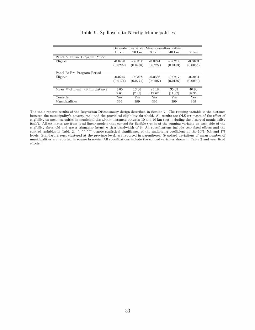
Table 9: Spillovers to Nearby Municipalities

Dependent variable: Mean casualties within:10 km 20 km 30 km 40 km 50 km

Panel A: Entire Program PeriodEligible -0.0280 -0.0317 -0.0274 -0.0214 -0.0103

(0.0222) (0.0256) (0.0227) (0.0153) (0.0085)

Panel B: Pre-Program PeriodEligible -0.0245 -0.0378 -0.0336 -0.0217 -0.0104

(0.0174) (0.0271) (0.0207) (0.0136) (0.0090)

Mean # of muni. within distance: 3.65 13.06 25.16 35.03 40.93[2.61] [7.85] [12.62] [11.87] [8.35]

Controls Yes Yes Yes Yes YesMunicipalities 399 399 399 399 399

The table reports results of the Regression Discontinuity design described in Section 2. The running variable is the distancebetween the municipality’s poverty rank and the provinical eligibility threshold. All results are OLS estimates of the effect ofeligibility on mean casualties in municipalities within distances between 10 and 40 km (not including the observed municipalityitself). All estimates are from local linear models that control for flexible trends of the running variable on each side of theeligibility threshold and use a triangular kernel with a bandwidth of 6. All specifications include year fixed effects and thecontrol variables in Table 2. ∗, ∗∗ ∗∗∗ denote statistical significance of the underlying coefficient at the 10%, 5% and 1%levels. Standard errors, clustered at the province level, are reported in parentheses. Standard deviations of mean number ofmunicipalities are reported in square brackets. All specifications include the control variables shown in Table 2 and year fixedeffects.

33

Figure 1: Map of KALAHI-CIDSS Municipalities

Black dots indicate municipalities that participated in KALAHI-CIDSS in the period 2003-2009.

Figure 2: The Effect of Eligibility on Participation

0.2

.4.6

.81

Pro

b. o

f par

ticip

atio

n in

KC

-6 -5 -4 -3 -2 -1 0 1 2 3 4 5 6Rank relative to cutoff

Mean Nonparametric fitQuadratic fit

The figure presents the relationship between the probability of participating in the KALAHI-CIDSS program and the runningvariable of the RD design, which is the distance between the municipality’s poverty rank and the provincial eligibility threshold.Scatter dots represent mean outcomes of bins with a width of 2 poverty ranks. The vertical bars are 95% confidence intervals.Dashed lines are quadratic fits, separately estimated on both sides of the eligibility threshold. Solid lines are nonparametricfits from a local linear regression that uses triangular kernels with a bandwidth of 6, separately estimated on both sides of theeligibility threshold.

34

Figure 3: The Effect of Eligibility on Casualties

.05

.1.1

5C

asua

lties

/mon

th



Entire Program Period

0.0

5.1

.15

Cas

ualti

es/m

onth



Pre-program

0.1

.2.3

.4C

asua

lties

/mon

th



Social preparation phase

.04

.06

.08

.1.1

2.1

4C

asua

lties

/mon

th



Remaining program period

The figure presents the relationship between the number of casualties experienced during the program period and the runningvariable of the RD design, which is the distance between the municipality’s poverty rank and the provincial eligibility threshold.Scatter dots represent mean outcomes of bins with a width of 2 poverty ranks. The vertical bars are 95% confidence intervals.Dashed lines are quadratic fits, separately estimated on both sides of the eligibility threshold. Solid lines are nonparametricfits from a local linear regression that uses triangular kernels with a bandwidth of 6, separately estimated on both sides of theeligibility threshold.

35

Figure 4: Robustness Tests for Continuity of Observables Across the Threshold

2000

025

000

3000

035

000

4000

0



Population

5060

7080



Fraction of villages with highay access

.1.2

.3.4



Ethnic fractionalization index

.15

.2.2

5.3

.35

.4-6 -5 -4 -3 -2 -1 0 1 2 3 4 5 6

Rank relative to cutoff


Religious fractionalization index

0.0

2.0

4.0

6.0

8.1



Percentage Muslim

.2.3

.4.5

.6.7



Affected by Insurgents

.2.3

.4.5

.6



Household access to electricity

.3.4

.5.6

.7



Household access to indoor plumbing

The figure presents the relationship between the running variable of the RD design, which is the distance between the munici-pality’s poverty rank and the provinical eligibility threshold, and a number of control variables. Scatter dots represent meansof bins with a bandwidth of 1. Dashed lines are quadratic fits, separately estimated on both sides of the eligibility threshold.Solid lines are nonparametric fits from a local linear regression that uses triangular kernels with a bandwidth of 6, separatelyestimated on both sides of the eligibility threshold.

36

Figure 5: Who Initiates the Violence and Who Suffers the Casualties?

.02

.04

.06

.08

.1C

asua

lties

/mon

th



Insurgent-initiated incidents

0.0

2.0

4.0

6.0

8C

asua

lties

/mon

th



Government-initiated incidents

.02

.04

.06

.08

.1C

asua

lties

/mon

th



Government Casualties

0.0

1.0

2.0

3.0

4.0

5C

asua

lties

/mon

th



Insurgent Casualties

0.0

1.0

2.0

3.0

4.0

5C

asua

lties

/mon

th



Civilian Casualties

The figure presents the relationship between the number of casualties experienced by different groups during the program periodand the running variable of the RD design, which is the distance between the municipality’s poverty rank and the provincialeligibility threshold. Scatter dots represent mean outcomes of bins with a width of 2 poverty ranks. The vertical bars are 95%confidence intervals. Dashed lines are quadratic fits, separately estimated on both sides of the eligibility threshold. Solid linesare nonparametric fits from a local linear regression that uses triangular kernels with a bandwidth of 6, separately estimatedon both sides of the eligibility threshold.

37

Figure 6: The Program’s Effect on Different Armed Groups

.02

.04

.06

.08

.1.1

2C

asua

lties

/mon

th



Incidents involving NPA

0.0

1.0

2.0

3.0

4C

asua

lties

/mon

th



Incidents involving MILF

0.0

2.0

4.0

6C

asua

lties

/mon

th



Incidents involving LE

The figure presents the relationship between the number of casualties experienced in incidients involving different armed groupsduring the program period and the running variable of the RD design, which is the distance between the municipality’s povertyrank and the provincial eligibility threshold. Scatter dots represent mean outcomes of bins with a width of 2 poverty ranks. Thevertical bars are 95% confidence intervals. Dashed lines are quadratic fits, separately estimated on both sides of the eligibilitythreshold. Solid lines are nonparametric fits from a local linear regression that uses triangular kernels with a bandwidth of 6,separately estimated on both sides of the eligibility threshold.

38

Figure 7: Spillover Effects

Program period

.04

.06

.08

.1.1

2.1

4M

ean

casu

altie

s/m

onth



Program PeriodCasualties within 10 km outside of muni.

.04

.06

.08

.1.1

2M

ean

casu

altie

s/m

onth




.04

.06

.08

.1.1

2M

ean

casu

altie

s/m

onth




.05

.06

.07

.08

.09

.1M

ean

casu

altie

s/m

onth




Pre-program period

.02

.04

.06

.08

Mea

n ca

sual

ties/

mon

th



Pre-program PhaseCasualties within 10 km outside of muni.

.04

.06

.08

.1.1

2M

ean

casu

altie

s/m

onth




.04

.06

.08

.1M

ean

casu

altie

s/m

onth




.05

.06

.07

.08

.09

Mea

n ca

sual

ties/

mon

th




The figure presents the relationship between the running variable of the RD design, which is the distance between the munici-pality’s poverty rank and the provinical eligibility threshold, and a number of control variables. Scatter dots represent meansof bins with a bandwidth of 1. Dashed lines are quadratic fits, separately estimated on both sides of the eligibility threshold.Solid lines are nonparametric fits from a local linear regression that uses triangular kernels with a bandwidth of 6, separatelyestimated on both sides of the eligibility threshold.

39

7 Appendix - for online publication

This appendix presents the results of a number of robustnes tests of our empirical approach.

7.1 Robustness Tests for Endogenous Timing

7.1.1 Results for Batch A Provinces Only

We first test for a possible effect of endogenous timing by reporting results for the subsample

of Batch A provinces only. As mentioned in Section 2 endogenous timing is not an issue

for municipalities in Batch A provinces, since all of them had the same start date for the

program and since this date was set before municipal eligibility was determined. Table 10

reports estimates of the effect of the KALAHI-CIDSS program on conflict in this subsample.

The results are similar to the ones for the entire sample reported in Table 4. The top panel

shows that the program had a positive and statistically significant effect on casualties in the

entire program period. The lower three panels show that this effect is due to a large and

statistically significant increase in casualties in the social preparation phase. There is no

statistically significant effect in the pre-program period and the later program period, after

the social preparation phase. The point estimates are similar to those for the whole sample,

though they are somewhat larger in the social preparation phase, which suggests that the

implementing agency may have timed the program in Batch B provinces to avoid conflict in

the social preparation phase.

7.1.2 Alternative Specification of the Start Date in Batch B Provinces

We now test for sensitivity to the use of August 2006 as the program’s start date in Batch

B provinces. For this test, we weight all observations in Batch B according to the ex-

ante probability with which municipalities were covered by the program at the time of the

40

observation. Out of the 117 municipalities that were covered in Batch B, 34 were covered in

Phase 3A, 29 in Phase 3B and the remaining 54 in Phase 4. We therefore assigned a weight

of 34117

to municipalities during the program period of Phase 3A, which started in October

2004, a weight of 29117

to observations during the period of Phase, which started in January

2006, and a weight of 54117

to observations in the program period of Phase 4, which started in

August 2006. Observations outside of the program period of any phase receive a weight of

zero. For observations that fall into the program period of several phases the weights were

assigned additively. For example, observations in March 2006, when Phases 3A and 3B were

both active, receive a weight of 34+29117

. As usual, we define the program period as ranging

from the start of the social preparation phase, 6 months before the program’s official start

date, until the end of the third program cycle, 36 months after the official start date. As

before, observations in Batch A provinces are included with a weight of 1 if they are in the

program period of Batch A and given a weight of 0 otherwise.

Table 11 shows that the results of this analysis is not substantially different from the results

of Table 4. The estimates that use probability weighting are slightly smaller, but similar

in magnitude and similarly statistically significant. There is therefore no evidence that our

results are driven by the choice of August 2006 as the program’s start date in Batch B

provinces.

7.2 Smoothness at “Pseudo-Thresholds”

We now test whether there are discontinuities in conflict casualties at other places away from

the threshold. Finding discontinuities at those “pseudo-thresholds”, where eligibility does

not change, would raise the concern that our results are due to mis-specified non-linearities in

the relationship between the running variable and the outcome Imbens and Lemieux (2008).

Following Imbens and Lemieux’s recommendation we look for discontinuities at two pseudo-

thresholds: the medians of the running variable for eligible and ineligible municipalities,

41

located at -2 and 3 relative poverty ranks, respectively. Table 13 shows that we find no

statistically significant evidence of discontinuities at these two thresholds.

7.3 Smoothness of Variables that Should not Have Been Affected

by KALAHI-CIDSS

As an additional robustness test, we test whether barely eligible and barely ineligible munic-

ipalites differed in outcomes during the program period that should not have been affected

by the program. Doing so is difficult in this context, since it is not easy to find data on such

outcomes in the Philippines. The most reliable municipality level data on relevant outcomes

comes from the Philippines National Census, which was only conducted in 2000, before the

program started, and in 2010, after the program had concluded. Given the data limitations,

we only test the program’s effect on household poverty incidence in the year 2003, which

was estimated by a World Bank study using a proxy means test. In 2003, the program

was active in Batch A provinces. Since the actual program implementation only began in

mid-2003, the program should not have affected household poverty yet. Finding an effect

would therefore indicate systematic differences in time-varying unobserved variables across

the eligibility threshold.

The results in Table 12 show no evidence of this. The program’s estimated effect on municipal

poverty incidence and poverty gap in 2003 are small and statistically insignificant. This result

is unchanged if we look only at Batch A provinces, in which the program was already active

in 2003.

42

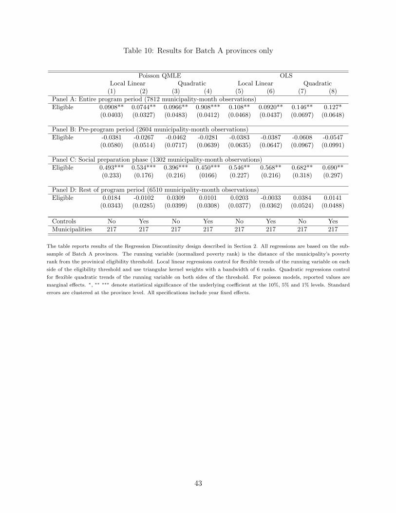
Table 10: Results for Batch A provinces only


(1) (2) (3) (4) (5) (6) (7) (8)Panel A: Entire program period (7812 municipality-month observations)Eligible 0.0908** 0.0744** 0.0966** 0.908*** 0.108** 0.0920** 0.146** 0.127*

(0.0403) (0.0327) (0.0483) (0.0412) (0.0468) (0.0437) (0.0697) (0.0648)

Panel B: Pre-program period (2604 municipality-month observations)Eligible -0.0381 -0.0267 -0.0462 -0.0281 -0.0383 -0.0387 -0.0608 -0.0547

(0.0580) (0.0514) (0.0717) (0.0639) (0.0635) (0.0647) (0.0967) (0.0991)

Panel C: Social preparation phase (1302 municipality-month observations)Eligible 0.493*** 0.534*** 0.396*** 0.450*** 0.546** 0.568** 0.682** 0.690**

(0.233) (0.176) (0.216) (0166) (0.227) (0.216) (0.318) (0.297)

Panel D: Rest of program period (6510 municipality-month observations)Eligible 0.0184 -0.0102 0.0309 0.0101 0.0203 -0.0033 0.0384 0.0141

(0.0343) (0.0285) (0.0399) (0.0308) (0.0377) (0.0362) (0.0524) (0.0488)


The table reports results of the Regression Discontinuity design described in Section 2. All regressions are based on the sub-

sample of Batch A provinces. The running variable (normalized poverty rank) is the distance of the municipality’s poverty

rank from the provinical eligibility threshold. Local linear regressions control for flexible trends of the running variable on each

side of the eligibility threshold and use triangular kernel weights with a bandwidth of 6 ranks. Quadratic regressions control

for flexible quadratic trends of the running variable on both sides of the threshold. For poisson models, reported values are

marginal effects. ∗, ∗∗ ∗∗∗ denote statistical significance of the underlying coefficient at the 10%, 5% and 1% levels. Standard

errors are clustered at the province level. All specifications include year fixed effects.

43

Table 11: Alternative Specification of Start Dates for Batch B Provinces


(1) (2) (3) (4) (5) (6) (7) (8)Panel A: Entire program period (14364 municipality-month observations)Eligible 0.0693*** 0.0673*** 0.0892*** 0.950*** 0.0748** 0.0685** 0.109** 0.103***

(0.0253) (0.0213) (0.0340) (0.0280) (0.0281) (0.0258) (0.0422) (0.0379)

Panel B: Pre-program period (4788 municipality-month observations)Eligible -0.0094 -0.0130 -0.0122 -0.0055 -0.0097 -0.0149 -0.0148 -0.0098

(0.0351) (0.0313) (0.0480) (0.0428) (0.0372) (0.0355) (0.0570) (0.0563)

Panel C: Social preparation phase (2394 municipality-month observations)Eligible 0.247*** 0.262*** 0.223** 0.248*** 0.291** 0.307** 0.369* 0.388**

(0.114) (0.0938) (0.114) (0.103) (0.131) (0.128) (0.183) (0.173)

Panel D: Rest of program period (11970 municipality-month observations)Eligible 0.0337 0.0264 0.0556* 0.0558** 0.0345 0.0235 0.0607* 0.0497

(0.0229) (0.0218) (0.0305) (0.0252) (0.0239) (0.0232) (0.0341) (0.0310)


The table reports results of the Regression Discontinuity design described in Section 2. All regressions use the weighting scheme

for the program’s start date described in Section 7.1.2. The running variable is the distance between the municipality’s poverty

rank and the provinical eligibility threshold. Local linear regressions control for flexible trends of the running variable on each

side of the eligibility threshold and use triangular kernel weights with a bandwidth of 6 ranks. Quadratic regressions control

for flexible quadratic trends of the running variable on both sides of the threshold. For poisson models, reported values are


errors are clustered at the province level. Control variables are shown in Table 2. All specifications include year fixed effects.

44

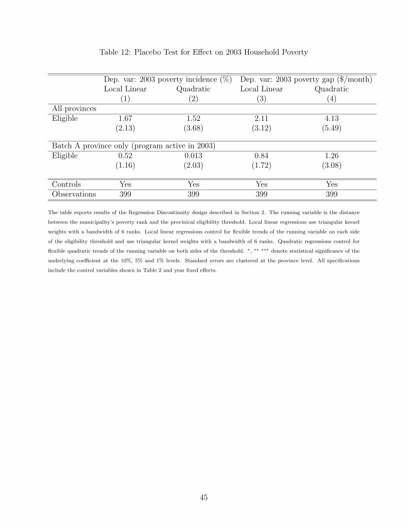
Table 12: Placebo Test for Effect on 2003 Household Poverty

Dep. var: 2003 poverty incidence (%) Dep. var: 2003 poverty gap ($/month)Local Linear Quadratic Local Linear Quadratic

(1) (2) (3) (4)All provincesEligible 1.67 1.52 2.11 4.13

(2.13) (3.68) (3.12) (5.49)

Batch A province only (program active in 2003)Eligible 0.52 0.013 0.84 1.26

(1.16) (2.03) (1.72) (3.08)

Controls Yes Yes Yes YesObservations 399 399 399 399


between the municipality’s poverty rank and the provinical eligibility threshold. Local linear regressions use triangular kernel

weights with a bandwidth of 6 ranks. Local linear regressions control for flexible trends of the running variable on each side

of the eligibility threshold and use triangular kernel weights with a bandwidth of 6 ranks. Quadratic regressions control for

flexible quadratic trends of the running variable on both sides of the threshold. ∗, ∗∗ ∗∗∗ denote statistical significance of the

underlying coefficient at the 10%, 5% and 1% levels. Standard errors are clustered at the province level. All specifications

include the control variables shown in Table 2 and year fixed effects.

45

Table 13: Robustness Test for Discontinuities at Pseudo-Thresholds

Dependent variable: Total casualties (entire program period)Poisson QMLE OLS

Local Linear Quadratic Local Linear Quadratic(1) (2) (3) (4)

Pseudo-threshold at -2 (median of eligible municipalities)Eligible 0.0322 0.0148 0.0416 0.0424

(0.0650) (0.187) (0.0949) (0.226)

Pseudo-threshold at 3 (median of ineligible municipalities)Eligible -0.0888 -0.0460 0.0031 -0.0304

(0.295) (0.0339) (0.0276) (0.0308)

Observations 14364 14364 14364 14364Municipalities 399 399 399 399


between the municipality’s poverty rank and pseudo-thresholds at -2.5 and 2.5 poverty ranks (the respectivemedians for eligible

and ineligible municipalities). Local linear regressions control for flexible trends of the running variable on each side of the

pseudo-threshold and use triangular kernel weights with a bandwidth of 6 ranks. Quadratic regressions control for flexible

quadratic trends of the running variable on both sides of the pseudo-threshold. For poisson models, reported values are


errors are clustered at the province level. All specifications include year fixed effects.

46

aid under fire: development projects and civil con ictneudc2012/docs/paper_268.pdf · aid under...

Documents