aic, cp and estimators of loss for elliptically symmetric ... · pdf filea. boisbunon et...

HAL Id: hal-00851206https://hal.archives-ouvertes.fr/hal-00851206

Submitted on 13 Aug 2013

HAL is a multi-disciplinary open accessarchive for the deposit and dissemination of sci-entific research documents, whether they are pub-lished or not. The documents may come fromteaching and research institutions in France orabroad, or from public or private research centers.

L’archive ouverte pluridisciplinaire HAL, estdestinée au dépôt et à la diffusion de documentsscientifiques de niveau recherche, publiés ou non,émanant des établissements d’enseignement et derecherche français ou étrangers, des laboratoirespublics ou privés.

AIC, Cp and estimators of loss for elliptically symmetricdistributions

Aurélie Boisbunon, Stephane Canu, Dominique Fourdrinier, WilliamStrawderman, Martin T. Wells

To cite this version:Aurélie Boisbunon, Stephane Canu, Dominique Fourdrinier, William Strawderman, Martin T. Wells.AIC, Cp and estimators of loss for elliptically symmetric distributions. 2013. <hal-00851206>

https://hal.archives-ouvertes.fr/hal-00851206

https://hal.archives-ouvertes.fr

AIC and Cp as estimators of loss for

spherically symmetric distributions∗

Aurelie Boisbunon, Stephane Canu, Dominique Fourdrinier,William Strawderman and Martin T. Wells

Abstract: In this article, we develop a modern perspective on Akaike’sInformation Criterion and Mallows’ Cp for model selection. Despite thedifferences in their respective motivation, they are equivalent in the specialcase of Gaussian linear regression. In this case they are also equivalent toa third criterion, an unbiased estimator of the quadratic prediction loss,derived from loss estimation theory. Our first contribution is to provide anexplicit link between loss estimation and model selection through a neworacle inequality. We then show that the form of the unbiased estimator ofthe quadratic prediction loss under a Gaussian assumption still holds undera more general distributional assumption, the family of spherically symmet-ric distributions. One of the features of our results is that our criterion doesnot rely on the specificity of the distribution, but only on its spherical sym-metry. Also this family of laws offers some dependence property betweenthe observations, a case not often studied.

Keywords and phrases: variable selection, Cp, AIC, loss estimator, un-biased estimator, SURE estimator, Stein identity, spherically symmetricdistributions.

1. Introduction

The problem of model selection has generated a lot of interest for many decadesnow and especially recently with the increased size of datasets. In such a context,it is important to model the data observed in a sparse way. The principle of par-simony helps to avoid classical issues such as overfitting or computational error.At the same time, the model should capture sufficient information in order tocomply with some objectives of good prediction, good estimation or good selec-tion and thus it should not be too sparse. This principle has been summarized bymany statisticians as a trade-off between goodness of fit to data and complexityof the model (see for instance Hastie, Tibshirani, and Friedman, 2008, Chapter7). From the practitioner point of view, model selection is often implementedthrough cross-validation (see Arlot and Celisse, 2010, for a review on this topic)or the minimization of criteria whose theoretical justification relies on hypoth-esis made within a given framework. In this paper, we review two of the mostcommonly used criteria, namely Mallows’ Cp and Akaike’s AIC, together withthe associated theory under Gaussian distributional assumptions, and then wepropose a generalization towards spherically symmetric distributions.

∗This research was partially supported by ANR ClasSel grant 08-EMER-002, by the SimonsFoundation grant 209035 and by NSF Grant DMS-12-08488.

1

A. Boisbunon et al./AIC and Cp as estimators of loss for spherical distributions 2

We will focus on the linear regression model

Y = Xβ + σε, (1)

where Y is a random vector in Rn, X is a fixed and known full rank designmatrix containing p observed variables xj in Rn, β is the unknown vector in Rpof regression coefficients to be estimated, σ is the noise level and ε is a randomvector in Rn representing the model noise, with mean zero and covariance matrixproportional to the identity matrix (we assume the proportion coefficient to beequal to one when ε is Gaussian). One subproblem of model selection is theproblem of variable selection: only a subset of the variables in X gives sufficientand non-redundant information on Y and we wish to recover this subset as wellas correctly estimate the corresponding regression coefficients.

Early works treated the model selection problem from the hypothesis testingpoint of view. For instance Forward Selection and Backward Elimination werestopped using Student’s critical values. This practice changed with Mallows’ au-tomated criterion known as Cp (Mallows, 1973). Mallows’ idea was to propose an

unbiased estimator of the scaled expected prediction error Eβ [‖XβI−Xβ‖2/σ2],

where βI is an estimator of β based on the selected variables set I ⊂ {1, . . . , p},Eβ denotes the expectation with respect to the sampling distribution in model(1) and ‖·‖ is the Euclidean norm on Rn. This way, assuming Gaussian i.i.d. er-ror terms, Mallows came to the following criterion

Cp =‖Y −XβI‖2

σ2+ 2df − n, (2)

where σ2 is an estimator of the variance σ2 based on the full linear model fittedwith the least-squares estimator βLS , that is, σ2 = ‖Y −XβLS‖2/(n−p), and dfis an estimator of df , the degrees of freedom, also called the effective dimensionof the model (see Hastie and Tibshirani, 1990; Meyer and Woodroofe, 2000).For the least squares estimator, df is the number k of variables in the selectedsubset I.

Mallows’ Cp relies on the assumption that, if for some subset I of explanatoryvariables the expected prediction error is low, then we can assume those variablesto be relevant for predicting Y. In practice, the rule for selecting the “best”candidate is the minimization of Cp. However, Mallows argues that this ruleshould not be applied in all cases, and that it is better to look at the shapeof the Cp-plot instead, especially when some explanatory variables are highlycorrelated.

In 1974, Akaike followed Mallows’ spirit to propose automatic criteria thatwould not need a subjective calibration of the significance level as in hypothesistesting. His proposal was more general with application to many problems suchas variable selection, factor analysis, analysis of variance, or order selection inauto-regressive models (Akaike, 1974). Akaike’s motivation however was differ-ent from Mallows. He considered the problem of estimating the density f(·|β)

of an outcome variable Y , where f is parametrized by β ∈ Rp, by f(·|β). Hisaim was to generalize the principle of maximum likelihood enabling a selection


between several maximum likelihood estimators βI . Akaike showed that all theinformation for discriminating f(·|βI) from f(·|β) could be summed up by the

Kullback-Leibler divergence DKL(βI , β) = E[log f(Ynew|β)] − E[log f(Ynew|βI)]where the expectation is taken over new observations. This divergence canin turn be approximated by its second-order variation when βI is sufficientlyclose to β, which actually corresponds to the distance ‖βI − β‖2I/2 whereI = −E[(∂2 log f/∂βi∂βj)

pi,j=1] is the Fisher-information matrix and for a vec-

tor z, its weighted norm ‖z‖I is defined by (ztIz)1/2. By means of asymptoticanalysis and by considering the expectation of DKL the author arrived at thefollowing criterion

AIC = −2

n∑i=1

log f(yi|βI) + 2k, (3)

where k is the number of parameters of βI . In the special case of a Gaussiandistribution, AIC and Cp are equivalent up to a constant for model (1) (seeSection 2.2). Hence Akaike described his AIC as a generalization of Cp for otherdistributional assumptions. Unlike Mallows, Akaike explicitly recommends therule of minimization of AIC to identify the best model from data. Note that Ye(1998) proposed to extend AIC to more complex settings by replacing k by the

estimated degrees of freedom df .Both Cp and AIC have been criticized in the literature, especially for the

presence of the constant 2 tuning the adequacy-complexity trade-off and fa-voring complex models in many situations, and many authors have proposedsome correction (see Schwarz (1978); Burnham and Anderson (2002); Fosterand George (1994); Shibata (1980)). Despite these critics, these criteria are stillquite popular among practicioners. Also they can be very useful in deriving bet-ter criteria of the form δ = δ0−γ, where δ0 is equal to Cp, AIC or an equivalentand γ is a correction function based on data. This framework, referred to asloss estimation, has been successfully used by Johnstone (1988) and Fourdrinierand Wells (1995), among others, to propose good criteria for selecting the bestsubmodel.

Another possible criticism of Cp and AIC regards their strong distributionalassumptions. Indeed, Cp’s unbiasedness has been shown under the Gaussiani.i.d. case, while AIC requires the specification of the distribution. However, inmany practical cases, we might not have any prior knowledge or intuition aboutthe form of the distribution, and we want the result to be robust to a widefamily of distributions.

The purpose of the present paper is twofold:

• First, we show in Section 2 that the procedures Cp and AIC are equiv-alent to unbiased estimators of the quadratic prediction loss when Y isassumed to be Gaussian in model (1). This result is an important ini-tial step for deriving improved criteria as is done in Johnstone (1988) andFourdrinier and Wells (2012). Both references consider the case of improv-ing the unbiased estimator of loss based on the data, which is consistentwith other approaches on data-driven penalties based on oracle inequali-


ties (see for instance Birge and Massart, 2007; Arlot and Massart, 2009).The derivation of better criteria will not be covered in the present article,but a relationship between oracle inequality and the statistical risk of theestimators of the prediction loss is provided section 2.2.2.

• Second, we derive the unbiased loss estimator for the wide family of spher-ically symmetric distributions and show that, for any spherical law, thisunbiased estimator is the same as that derived under the Gaussian law.The family of spherically symmetric distribution is a large family whichgeneralizes the multivariate standard normal law and includes multivari-ate versions of the Student, Cauchy, Kotz, and Pearson type II and typeVII distributions among others. Also, the spherical assumption frees usfrom the independence assumption of the error terms in (1), while not re-jecting it since the Gaussian law is spherical. Note however that sphericalsymmetry here means no correlation, the case of correlated observationsbeing handled by elliptical symmetry. Furthermore, some members of thespherical family, like the Student law, have heavier tails than the Gaussiandensity allowing a better handling of potential outliers. Finally, the resultsof the present work do not depend on the specific form of the distribution.The last two points provide some distributional robustness.

2. Expression of AIC and Cp in the loss estimation framework

2.1. Basics of loss estimation

2.1.1. Unbiased loss estimation

The idea underlying the estimation of loss is closely related to Stein’s UnbiasedRisk Estimate (SURE, Stein, 1981). The theory of loss estimation was initiallydeveloped for problems of estimation of the location parameter of a multivariatedistribution (see e.g. Johnstone, 1988; Fourdrinier and Strawderman, 2003). Theprinciple is classical in statistics and goes as follow: we wish to evaluate theaccuracy of a decision rule µ for estimating the unknown location parameter µ(in the linear model (1), we have µ = Xβ). Therefore we define a loss function,which we write L(µ, µ), measuring the discrepancy between µ and µ. A typicalexample is the quadratic loss L(µ, µ) = ‖µ− µ‖2. Since L(µ, µ) depends on theunknown parameter µ, it is unknown as well and can thus be assessed throughan estimation using the observations (see for instance Fourdrinier and Wells(2012) and references therein for more details on loss estimation). The maindifference with classical approaches (such as SURE) is that we are interested inestimating the actual loss, not its expectation, that is the risk

R(µ, µ) := Eµ[L(µ, µ)]. (4)

In this paper we only consider unbiasedness as our notion of optimality. Hence,let us start with the definition of an unbiased estimator of loss in a generalsetting. This definition of unbiasedness is the one used by Johnstone (1988).


Definition 1 (Unbiasedness). Let Y be a random vector in Rn with mean µ ∈Rn, and let µ be any estimator of µ. An estimator δ0(Y ) of the loss L(µ, µ) issaid to be unbiased if, for all µ ∈ Rn,

Eµ[δ0(Y )] = Eµ[L(µ, µ)]

where Eµ denotes the expectation with respect to the distribution of Y .

This definition of unbiasedness of an estimator of the loss is somehow nonstandard. The usual notion of unbiasedness is retrieved when considering δ0(Y )as an estimator of the risk R(µ, µ) since the risk is the expectation of the loss,see (4). However, this terminology of loss estimation, due to Sandved (1968) andLi (1985), has been used by other authors (among others Johnstone (1988); Lele(1993); Fourdrinier and Strawderman (2003); Fourdrinier and Wells (2012)). Dif-ferences between loss estimation and risk estimation are enlightened by resultsfrom Li (1985). Li proves that SURE estimates the loss consistently over thetrue mean µ as n goes to infinity. He also constructs a simple example where µis estimated by a particular form of James-Stein shrinkage estimators for whichSURE tends asymptotically to a random variable, and hence is inconsistent forthe estimation of the risk, which is not random. Another interesting result of Li(1985) is the consistency of the estimator of µ selected using the rule “minimizeSURE” (which is equivalent to the rule “minimize the unbiased estimator δ0”).Although this result has only been proved for the special case of James-Steintype estimators, this is encouraging for choosing such a rule to select the bestmodel from data.

Although in practice SURE and unbiased loss estimators are the same, webelieve this discussion makes it clear that the actual loss is a more relevant quan-tity of interest than the risk. The difference will be important when improvingon unbiased estimators, as we will discuss in the perspectives of Section 4.

Obtaining an unbiased estimator of loss requires Stein’s identity, the key the-orem of loss estimation theory which we recall here for the sake of completenessand whose proof can be found in Stein (1981).

Theorem 1 (Stein’s identity). Let Y ∼ Nn(µ, σ2In). Given g : Rn → Rna weakly differentiable function, we have, assuming the expectations exist, thefollowing equality

Eµ[(Y − µ)tg(Y )

]= σ2 Eµ [divY g(Y )] , (5)

where divY g(Y ) =∑ni=1 ∂gi(Y )/∂Yi is the weak divergence of g(Y ) with respect

to Y .

See e.g. Section 2.3 in Fourdrinier and Wells (1995) for the definition and thejustification of weak differentiability.

2.1.2. Unbiased loss estimation for model (1)

When considering the Gaussian model in (1), we have µ = Xβ, we set µ = Xβ

and L(β, β) is defined as the quadratic loss ‖Xβ −Xβ‖2. Special focus will be


given to the quadratic loss since it is the most commonly used and allows simplecalculations. In practice, it is a reasonable choice if we are interested in bothgood selection and good prediction at the same time. Moreover, the quadraticloss allows us to link loss estimation with Cp and AIC.

In the following theorem, an unbiased estimator of the quadratic loss undera Gaussian assumption is provided.

Theorem 2. Let Y ∼ Nn(Xβ, σ2In). Let β = β(Y ) be a function of the least

squares estimator of β such that Xβ is weakly differentiable with respect to Y .Let σ2 = ‖Y −XβLS‖2/(n− p). Then

δ0(Y ) = ‖Y −Xβ‖2 + (2 divY (Xβ)− n)σ2 (6)

is an unbiased estimator of ‖Xβ −Xβ‖2.

Proof. The risk of Xβ at Xβ is

Eβ [‖Xβ −Xβ‖2] = Eβ [‖Xβ − Y ‖2 + ‖Y −Xβ‖2] (7)

+Eβ [2(Y −Xβ)t(Xβ − Y )].

Since Y ∼ Nn(Xβ, σ2In), we have Eβ [‖Y −Xβ‖2] = nσ2 leading to

Eβ [‖Xβ −Xβ‖2]=Eβ [‖Y −Xβ‖2]− nσ2 + 2 tr(covβ(Xβ, Y −Xβ)).

Moreover, applying Stein’s identity for the right-most part of the expectation in(7) with g(Y ) = Xβ and assuming that Xβ is weakly differentiable with respectto Y , we can rewrite (7) as

Eβ [‖Xβ −Xβ‖2] = Eβ [‖Y −Xβ‖2]− nσ2 + 2σ2 Eβ[divYXβ

].

Since σ2 is an unbiased estimator of σ2 independent of βLS , the right-handside of this last equality is also equal to the expectation of δ0(Y ) given byEquation (6). Hence, according to Definition 1, the statistic δ0(Y ) is an unbiased

estimator of ‖Xβ −Xβ‖2.

Remark 1. It is often of interest to use robust estimators of β and σ2. In such acase, the hypotheses of the theorem need to be modified to insure the independencebetween estimators β and σ2 which were implicit in the statement of the theorem.We will see in Remark 2 of the next section that, by the use of Stein identity forthe general spherical case, the implicit assumption of independence is no longerneeded.

In the following subsections, we discuss our choices for the measure of com-plexity of a model (through the divergence term) and for the estimation of thevariance, and we relate them to other choices from the literature.


2.1.3. Degrees of freedom

It turns out that the divergence term of δ0(Y ) in (6), divYXβ, is related to the

estimator of the degrees of freedom df used in Equation (2) for the definition ofCp, and to the number k of parameters proposed for AIC in (3).

A convenient way to establish this connection is to follow Ye (1998) in definingthe (generalized) degrees of freedom of an estimator as the trace of the scaled

covariance between the prediction Xβ and the observation Y

df =1

σ2tr(

covβ(Xβ, Y )). (8)

This definition has the advantage of encompassing the effective degrees of free-dom proposed for generalized linear models and the standard degrees of freedomused when dealing with the least squares estimator.

When it applies, Stein’s identity yields

df = Eβ [divYXβ].

Settingdf = divYXβ,

the statistic df appears as an unbiased estimator of the (generalized) degrees offreedom. In the case of linear estimators, there exists a hat matrix, that is, amatrix H such that Xβ = HY and we have

divYXβ = divY (HY ) =

n∑i=1

∂∑nj=1Hi,jYj

∂Yi=

n∑i=1

Hi,i = tr(H),

so thatdf = tr(H).

This definition of df is the one used by Mallows for the extension of Cp to ridge

regression. Note that, in this case, df no longer depends on Y and thus equalsits expectation (df = df). When H is a projection matrix (i.e. when H2 = H)as it is for the least squares estimator, then we have

tr(H) = k,

where k is the rank of the projector which is also the number of linearly inde-pendent parameters, and thus df = k.

In this case the definition of degrees of freedom agrees with intuition. It isthe number of parameters of the model that are free to vary. When H is nolonger a projector, rank(H) is no longer a valid measure of complexity sinceit can be equal to n while for admissible estimators tr(H) is the trace normof H (also known as the nuclear norm). The trace norm is also the minimumconvex envelope of rank(H) over the unit ball of the spectral norm, used asa convex proxy for the rank in some optimization problem (see for instance


Recht, Fazel, and Parrilo (2010) and the references therein). As a convex norm,tr(H) is a continuous measure of the complexity of the associated mapping. For

nonlinear estimators, the divergence divYXβ is the trace of the Jacobian matrix(its nuclear norm) of the mapping that produced a set of fitted values for Y .According to Ye (1998), it can be interpreted as “the cost of the estimationprocess” or as “the sum of the sensitivity of each fitted value to perturbations”.

Other measures of the complexity, involving the trace or the determinantof the Fisher information matrix I, have been used for instance by Takeuchi(1976) and Bozdogan (1987). However, such measures depend on the specificform of the distribution considered which does not suit our context. The Vapnik-Chervonenkis dimension (VC-dim, Vapnik and Chervonenkis (1971)), is anotherway to capture the complexity of the model. However, it can be difficult tocompute for nonlinear estimators while it is equivalent to our divergence termfor linear estimators. Hence, Cherkassky and Ma (2003) proposed to estimate

the VC-dim by df .

2.1.4. Estimators of the variance

The issue of estimating the variance was clearly pointed out in Cherkassky andMa (2003). The authors proposed two estimators of the variance, one for the

full model together with βLS the least-squares estimator

σ2full =

‖Y −XβLS‖2

n− p, (9)

and the second one for the model restricted to a subset I ⊂ {1, . . . , p}

σ2restricted =

‖Y −XβI‖2

n− k, (10)

where k is the size of I and βI is linear in Y . Note that other estimators of σ2 canbe found in the literature (see for instance Arlot and Bach, 2009). As mentionedearlier, we are concerned with unbiasedness of the loss, so that the estimator ofσ2 should be unbiased and independent of divYXβ. Hence the choice betweenσ2full and σ2

restricted should be made with respect to what we believe is the truemodel, either the full model in (1) or the restricted model

Y = XIβI + σ ε.

In the general case where βI is not necessarily linear in Y , the variance is usuallyestimated by (10) where k is replaced by df . However, in such a case, it is notclear whether this estimator is independent of Y or not. Also, the use of σ2

restricted

might not lead to an equivalence between the unbiased estimator of loss (24)and AIC. Indeed, in such a case the unbiased estimator of loss would have theform k‖ Y −XβI‖2/(n− k), while AIC would result in log σ2

restricted + 2k. Thisis just model selection based on the minimum standard error. On the contrary,when considering the estimator σ2

full, the equivalence is pretty clear, as we willsee in the next section.


2.2. Links between loss estimation and model selection

2.2.1. Selection criteria

In order to make the following discussion clearer, we recall here the formula ofthe three criteria of interest for the Gaussian assumption, namely the unbiasedestimator of loss δ0(Y ), Mallows’ Cp and the extended version of AIC proposedby Ye (1998):

δ0(Y ) = ‖Y −Xβ‖2 + (2 divY (Xβ)− n)σ2

Cp =‖Y −Xβ‖2

σ2+ 2 divY (Xβ)− n

AIC =‖Y −Xβ‖2

σ2+ 2 divY (Xβ).

Using the estimator σ2full of the variance in (9), we thus obtain the following

link between δ0, Cp and AIC:

δ0(Y ) = σ2full × Cp = σ2

full × (AIC− n). (11)

These links between different criteria function for model selection are dueto the fact that, under our working hypothesis (linear model, quadratic loss,normal distribution Y ∼ Nn(Xβ, σ2In) for a fixed design matrix X), they canbe seen as unbiased estimators of related quantities of interest.

Note that there is also an equivalence with other model selection criteria,investigated for instance in Li (1985), Shao (1997) and Efron (2004).

2.2.2. Quality of model selection procedures

Given a loss estimator L(βI , β) (such as δ0), the corresponding model selectionprocedure consists in finding the best subset of variables, I, that is,

I = arg minI

L(βI , β)

where βI is the chosen estimator associated to the subset I of variables. To assessthe quality of this model selection procedure, from a nonasymptotic point of view(fixed n), Donoho and Johnstone (1994) introduced the notion of an oracle. Anoracle is supposed to determine the ideal subset, I?, that is,

I? = arg minI

L(βI , β).

A good model selection procedure approaches the ideal performance. More for-mally, the associated oracle inequality states that, with high probability,

L(βI , β) ≤ L(βI? , β) + ε. (12)


That is to say for any α, 0 < α < 1, there is a positive ε such that

P(L(βI , β)− L(βI? , β) ≥ ε

)≤ α. (13)

Noticing that L(βI , β) ≤ L(βI? , β) we can write

P(L(βI , β)− L(βI? , β) ≥ ε

)≤ P

(|L(βI? , β)− L(βI? , β)| ≥ ε

2

)+ P

(|L(βI , β)− L(βI , β)| ≥ ε

2

)≤

∑I

P(|L(βI , β)− L(βI , β)| ≥ ε

2

)considering all the subsets I. Then by Chebyshev’s inequality

P(L(βI , β)− L(βI? , β) ≥ ε

)≤

∑I

4

ε2E[|L(βI , β)− L(βI , β)|2

]=

4

ε2

∑I

R(L(βI , β)

),

where R(L(βI , β)

)is the statistical risk of a further quadratic loss function

R(L(βI , β)

):= E

[|L(βI , β)− L(βI , β)|2

]. (14)

Hence, for any α we can find ε, say,

ε = 2

√√√√∑I

R(L(βI , β)

)α

(15)

such that the oracle inequality (12) is satisfied. It is clear that a way of con-trolling the oracle bound of the selector is to choose a loss estimator with smallquadratic risk. In the case where the loss estimator is of the form squared resid-ual plus a penalty function the oracle condition above translates into a sufficientcondition on the behavior of the penalty term. Classical oracle inequality anal-ysis gives an exponential bound on the left-hand side of (13). The developmentof such a result requires a concentration type inequality for the maximum ofGaussian processes (see Massart (2007)) to give an exponential upper bound on(12) that tends to zero. Our goal here is complementary to the standard oracleinequality approach; that is, we developed a novel upper bound that links thequality of the model selection procedure to the risk assessment of a loss estima-tor. This idea is further elucidated in Barron, Birge, and Massart (1999); Birgeand Massart (2007) and related work. Note that, in particular, Cp has beenproven to satisfy an oracle inequality by Baraud (2000).

Bartlett, Boucheron, and Lugosi (2002) studied model selection strategiesbased on penalized empirical loss minimization in the context of bounded loss.


They prove, using concentration inequality techniques, the equivalence betweenloss estimation and data-based complexity penalization. It was shown that goodloss estimates may be converted into a data-based penalty function and theperformance of the estimate is governed by the quality of the loss estimate.Furthermore, it was shown that a selected model that minimizes the empiricalloss achieves an almost optimal trade-off between the approximation error andthe expected complexity. The key point to stress is that the results of Bartlettet al. are concordant with the oracle bound in (15), that is there is a fundamentaldependence on the notions of good complexity regularization and good lossestimation.

2.2.3. Model selection

The final objective is to select the “best” model among those at hand. This canbe performed by minimizing either of the three proposed criteria, that is theunbiased estimator of loss δ0, Cp and AIC. The idea behind this heuristic, asshown in the previous section, is that the best model in terms of prediction isthe one minimizing the estimated loss. Now, from (11), it can be easily seenthat the three criteria differ from each other only up to a multiplicative and/oradditive constant. Hence the models selected by the three criteria will be thesame.

We would like to point out that Theorem 2 does not rely on the linearity ofthe link between X and Y so that this work can easily be extended to nonlinearlinks at no extra cost. Therefore δ0 generalizes Cp to nonlinear models. Moreover,following its definition (3), AIC implementation requires the specification of theunderlying distribution. In this sense it is considered as a generalization of Cp fornon Gaussian distributions. However, in practice, we might only have a vagueintuition of nature of the underlying distribution and we might not be ableto give its specific form. We will see in the following section that δ0, which isequivalent to the Gaussian AIC as we have just seen, can be also derived from amore general distribution context, that of spherically symmetric distributions,with no need to specify the precise form of the distribution.

3. Unbiased loss estimators for spherically symmetric distributions

3.1. Multivariate spherical distributions

In the previous section, results were given under the Gaussian assumption withcovariance matrix σ2In. In this section, we extend this distributional framework.

The characterization of the normal distribution as expressed by Kariya andSinha (1989) allows two directions for generalization. Indeed, the authors assertthat a random vector is Gaussian, with covariance matrix proportional to theidentity matrix, if and only if its components are independent and its law isspherically symmetric. Hence, we can generalize the Gaussian assumption by


either keeping the independence property and consider other laws than theGaussian, or by relaxing the independence assumption to the benefit of sphericalsymmetry. In the same spirit, Fan and Fang (1985) pointed out that thereare two main generalizations of the Gaussian assumption in the literature: onegeneralization comes from the interesting properties of the exponential formand leads to the exponential family of distributions, while the other is basedon the invariance under orthogonal transformation and results in the familyof spherically symmetric distributions (which can be generalized by ellipticallycontoured distributions). These generalizations go in different directions andhave lead to fruitful works. Note that their only common member is the Gaussiandistribution. The main interest of choosing spherical distributions is that theconjunction of invariance under orthogonal transformation together with linearregression with less variables than observations brings robustness. The interestof that property is illustrated by the fact that some statistical tests designedunder a Gaussian assumption, such as Student and Fisher tests, remain valid forspherical distributions Wang and Wells (2002); Fang and Anderson (1990). Thisrobustness property is not shared by independent non-Gaussian distributions,as mentioned in Kariya and Sinha (1989).

Note that, from the model in (1), the distribution of Y is the distribution ofσ ε translated by µ = Xβ: Y has a spherically symmetric distribution about thelocation parameter µ with covariance matrix equal to n−1σ2E[‖ε‖2]In where Inis the identity matrix. We write ε ∼ Sn(0, In) and Y ∼ Sn(µ, σ2In). Examplesof this family besides the Gaussian distribution Nn are the Student distributionTn, the Kotz distribution Kn, or else variance mixtures of Gaussian distributionsGMn whose densities are respectively given by

Nn(y;µ, σ2) =1

(2πσ2)n/2e−‖y−µ‖2

2σ2

Tn(y;µ, σ2, ν) =Γ[(n+ ν)/2]

(πσ2)n/2Γ(ν/2)νn/2

[1 +‖y − µ‖2

νσ2

]− (ν+n)2

Kn(y;µ, σ2, N, r)=Γ(n/2)rN−1+n/2

πn2 σn+2−2NΓ

(N − 1 + n

2

)‖y − µ‖2(N−1)e−r ‖y−µ‖2σ2

GMn(y;µ, σ2, G) =1

(2πσ2)n/2

∫ ∞0

1

vn/2e−‖y−µ‖2

2vσ2 G(dv) ,

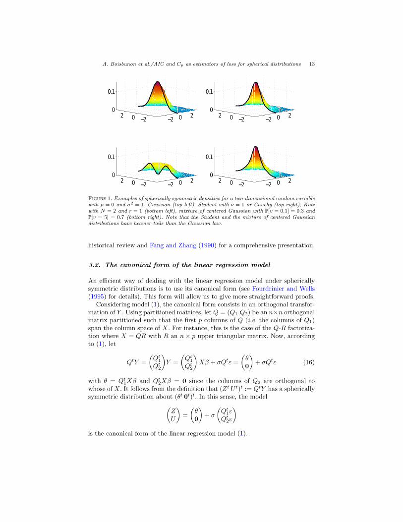
where ν ≥ 1, 2N + n > 2, r > 0, and G(·) is a probability measure on the scaleparameter v. Here, Γ denotes the Gamma function. Note that the Gaussiandistribution is a special case of Kotz distribution with r = 1/2 and N = 1,and of Gaussian mixtures, while it is the limiting distribution of the Studentlaw when ν tends to infinity. Figure 1 shows the shape of these densities in twodimensions (n = 2).

As we will see in the sequel, the unbiased estimator of the quadratic loss δ0(24) remains unbiased for any of these distributions with no need to specify itsform. It thus brings distributional robustness. For more details and examples ofthe spherical family, we refer the interested reader to Chmielewski (1981) for a


−2 0 2−202

0

0.1

−2 0 2−202

0

0.1

−2 0 2−202

0

0.1

−2 0 2−202

0

0.1

Figure 1. Examples of spherically symmetric densities for a two-dimensional random variablewith µ = 0 and σ2 = 1: Gaussian (top left), Student with ν = 1 or Cauchy (top right), Kotzwith N = 2 and r = 1 (bottom left), mixture of centered Gaussian with P[v = 0.1] = 0.3 andP[v = 5] = 0.7 (bottom right). Note that the Student and the mixture of centered Gaussiandistributions have heavier tails than the Gaussian law.

historical review and Fang and Zhang (1990) for a comprehensive presentation.

3.2. The canonical form of the linear regression model

An efficient way of dealing with the linear regression model under sphericallysymmetric distributions is to use its canonical form (see Fourdrinier and Wells(1995) for details). This form will allow us to give more straightforward proofs.

Considering model (1), the canonical form consists in an orthogonal transfor-mation of Y . Using partitioned matrices, let Q = (Q1 Q2) be an n×n orthogonalmatrix partitioned such that the first p columns of Q (i.e. the columns of Q1)span the column space of X. For instance, this is the case of the Q-R factoriza-tion where X = QR with R an n× p upper triangular matrix. Now, accordingto (1), let

QtY =

(Qt1Qt2

)Y =

(Qt1Qt2

)Xβ + σQtε =

(θ0

)+ σQtε (16)

with θ = Qt1Xβ and Qt2Xβ = 0 since the columns of Q2 are orthogonal towhose of X. It follows from the definition that (Zt U t)t := QtY has a sphericallysymmetric distribution about (θt 0t)t. In this sense, the model(

ZU

)=

(θ0

)+ σ

(Qt1εQt2ε

)is the canonical form of the linear regression model (1).


This canonical form has been considered by various authors such as Cel-lier, Fourdrinier, and Robert (1989); Cellier and Fourdrinier (1995); Maruyama(2003); Maruyama and Strawderman (2005, 2009); Fourdrinier and Strawder-man (2010); Kubokawa and Srivastava (1999). Kubokawa and Srivastava (2001)addressed the multivariate case where θ is a mean matrix (in this case Z and Uare matrices as well).

For any estimator β, the orthogonality of Q implies that

‖Y −Xβ‖2 = ‖θ − Z‖2 + ‖U‖2 (17)

where θ = Qt1Xβ is the corresponding estimator of θ. In particular, for the least

squares estimator βLS , we have

‖Y −XβLS‖2 = ‖U‖2. (18)

In that context, we recall the Stein-type identity given by Fourdrinier andWells (1995).

Theorem 3 (Stein-type identity). Given (Z,U) ∈ Rn a random vector followinga spherically symmetric distribution around (θ,0), and g : Rp → Rp a weaklydifferentiable function, we have

Eθ[(Z − θ)tg(Z)] = Eθ[‖U‖2divZg(Z)/(n− p)], (19)

provided both expectations exist.

Note that the divergence in Theorem 2 is taken with respect to Y whilethe Stein type identity (19) requires the divergence with respect to Z (withthe assumption of weak differentiability). Their relationship can be seen in thefollowing lemma.

Lemma 1. We have

divYXβ(Y ) = divZ θ(Z,U) . (20)

Proof. Denoting by tr(A) the trace of any matrix A and by Jf (x) the Jacobianmatrix (when it exists) of a function f at x, we have

divYXβ(Y ) = tr(JXβ(Y )

)= tr

(Qt JXβ(Y )Q

)by definition of the divergence and since Qt is an orthogonal matrix. Now,setting W = Qt Y , i.e. Y = QW , applying the chain rule to the function

T (W ) = QtXβ(QW )

gives rise toJT (W ) = JQtXβ(Y )Q = Qt JXβ(Y )Q, (21)

noticing that Qt is a linear transformation.


Also, as according to (16)

W =

(ZU

)and T =

(θ0

),

the following decomposition holds

JT (W ) =

(Jθ(Z) Jθ(U)

0 0

),

where Jθ(Z) and Jθ(U) are the parts of the Jacobian matrix in which the deriva-tives are taken with respect to the components of Z and U respectively. Thus

tr(JT (W )

)= tr

(Jθ(Z)

)(22)

and, therefore, gathering (21) and (22), we obtain

tr(Jθ(Z)

)= tr

(Qt JXβ(Y )Q

)= tr

(QQt JXβ(Y )

)= tr

(JXβ(Y )

),

which is (20) by definition of the divergence.

3.3. Unbiased estimator of loss for the spherical case

This section is devoted to the generalization of Theorem 2 to the class of spher-ically symmetric distributions Y ∼ Sn(Xβ, σ2), given by Theorem 4. To do sowe need to consider the statistic

σ2(Y ) = 1n−p‖Y −Xβ

LS‖2. (23)

It is an unbiased estimator of σ2Eβ [‖ε‖2/n]. Note that, in the normal case whereY ∼ Nn(Xβ, σ2In), we have Eβ [‖ε‖2/n] = 1 so that σ2(Y ) is an unbiasedestimator of σ2.

Theorem 4 (Unbiased estimator of the quadratic loss under spherical assump-

tion). Let Y ∼ Sn(Xβ, σ2In) and let β = β(Y ) be an estimator of β depending

only on Qt1Y . If β(Y ) is weakly differentiable with respect to Y , then the statistic

δ0(Y ) = ‖Y −Xβ(Y )‖2 + (2 divY (Xβ(Y ))− n) σ2(Y ) , (24)

is an unbiased estimator of ‖Xβ(Y )−Xβ‖2.

Proof. The quadratic loss function of Xβ at Xβ can be decomposed as

‖Xβ −Xβ‖2 = ‖Y −Xβ‖2 + ‖Y −Xβ‖2 + 2 (Xβ − Y )t(Y −Xβ) . (25)

The expectation of the second term in the right hand side of (25) has beenconsidered in (23). As for the third term, by orthogonally invariance of the


inner product,

(Xβ − Y )t(Y −Xβ) = (QtXβ −QtY )t(QtY −QtXβ)

=

(Qt1Xβ −Qt1YQt2Xβ −Qt2Y

)t(Qt1Y −Qt1XβQt2Y −Qt2Xβ

)=

(θ − Z−U

)t(Z − θU

)= (θ − Z)t(Z − θ)− ‖U‖2 . (26)

Now, since θ = θ(Z,U) depends only on Z, by Stein type identity, we have

E[(θ − Z)t(Z − θ)

]= E

[‖U‖2

n− pdivZ(θ − Z)

]= E

[‖U‖2

n− p

(divZ θ − p

)](27)

so that

E[(Xβ − Y )t(Y −Xβ)] = E[‖U‖2

n− p

(divZ θ − p

)− ‖U‖2

]= E

[‖U‖2

n− pdivZ θ −

n

n− p‖U‖2

]= E[σ2(Y ) divYXβ − n σ2(Y )] (28)

by (18) and since divZ θ = divYXβ by Lemma 1. Finally, gathering (25), (23)and (28) gives the desired result.

From the equivalence between δ0, Cp and AIC under a Gaussian assumption,and the unbiasedness of δ0 under the wide class of spherically symmetric distri-butions, we conclude that Cp and AIC derived under the Gaussian distributionstill can be considered as good selection criteria for spherically symmetric dis-tributions, although their original properties may not have been verified in thiscontext.

Remark 2. Note that the extension of Stein’s lemma in Theorem 3 implies thatdf = divYXβ is also an unbiased estimator of df under the spherical assump-tion. Moreover, we would like to point out that the independence of σ2 used inthe proof of Theorem 2 in the Gaussian case is no longer necessary. Also, to re-quire that β depends on Qt1Y only is equivalent to say that β is a function of theleast squares estimator. When this hypothesis is not available, an extended Steintype identity can be derived (Fourdrinier, Strawderman, and Wells (2003)).

4. Discussion

In this work, we studied the well-known model selection criteria Cp and AICthrough a loss estimation approach and related them to an unbiased estimator


of the quadratic prediction loss under a Gaussian assumption. We then derivedthe unbiased estimator of loss under a wider distributional setting, the family ofspherically symmetric distributions. Under this context, the unbiased estimatorof loss is actually equal to the one derived under the Gaussian law. Hence, thisimplies that we do not have to specify the form of the distribution, the onlycondition being its spherical symmetry. We also conclude from the equivalencebetween unbiased estimators of loss, Cp and AIC that their form for the Gaus-sian case is able to handle any spherically symmetric distribution. The sphericalfamily is interesting for many practical cases since it allows a dependence prop-erty between the components of random vectors whenever the distribution is notGaussian. Some members of this family also have heavier tails than the Gaus-sian law, and thus the unbiased estimator derived here can be robust to outliers.A generalization of this work with elliptically symmetric distributions for theerror vector would go even further by taking into account a general covariancematrix Σ. We intend to study this case in future work.

It is well known that unbiased estimators of loss are not the best estimatorsand can be improved. It was not our intention in this work to show betterresults of such estimators, but our result explains why their performances canbe similar when departing from the Gaussian assumption. The improvementof these unbiased estimators requires a way to assess their quality. This canbe done either using oracle inequalities or the theory of admissible estimatorsunder a certain risk. These two points of view are closely related. Based on ourdefinition of the risk (14) a selection rule δ0 is inadmissible if we can find abetter estimator, say δγ , that has a smaller risk function for all possible valuesof the parameter β, that is, with stict inequality for some β. The heuristic ofloss estimation is that the closer an estimator is to the true loss, the morewe expect their respective minima to be close. We are currently working onimproved estimators of loss of the type δγ(Y ) = δ0(Y ) + γ(Y ), where γ − 2kσcan be thought of as a data driven penalty. From another point of view, choosinga γ improvement term, decreases the oracle bound given in (15). The selectionof such a γ term is an important research direction.

References

H. Akaike. A new look at the statistical model identification. IEEE Transactionson Automatic Control, 19(6):716–723, 1974.

S. Arlot and F. Bach. Data-driven calibration of linear estimators with minimalpenalties. In Y. Bengio, D. Schuurmans, J. Lafferty, C. K. I. Williams, andA. Culotta, editors, Advances in Neural Information Processing Systems 22,pages 46–54. NIPS, 2009.

S. Arlot and A. Celisse. A survey of cross-validation procedures for modelselection. Statistics Surveys, 4:40–79, 2010.

S. Arlot and P. Massart. Data-driven calibration of penalties for least-squaresregression. Journal of Machine Learning Research, 10:245–279, 2009.

Y. Baraud. Model selection for regression on a fixed design. Probability Theoryand Related Fields, 117(4):467–493, 2000.


A. Barron, L. Birge, and P. Massart. Risk bounds for model selection viapenalization. Probability theory and related fields, 113(3):301–413, 1999.

P.L. Bartlett, S. Boucheron, and G. Lugosi. Model selection and error estima-tion. Machine Learning, 48(1):85–113, 2002.

L. Birge and P. Massart. Minimal penalties for Gaussian model selection. Prob-ability Theory and Related Fields, 138(1):33–73, 2007.

H. Bozdogan. Model selection and Akaike’s information criterion (AIC): Thegeneral theory and its analytical extensions. Psychometrika, 52(3):345–370,1987.

K.P. Burnham and D.R. Anderson. Model Selection and Multimodel Inference:a Practical Information-Theoretic Approach. Springer Verlag, 2002.

D. Cellier and D. Fourdrinier. Shrinkage estimators under spherically symmetryfor the general linear model. Journal of Multivariate Analysis, 52:338–351,1995.

D. Cellier, D. Fourdrinier, and C. Robert. Robust shrinkage estimators of thelocation parameter for elliptically symmetric distributions. Journal of Multi-variate Analysis, 29:39–52, 1989.

V. Cherkassky and Y. Ma. Comparison of model selection for regression. NeuralComputation, 15(7):1691–1714, 2003.

M.A. Chmielewski. Elliptically symmetric distributions: A review and bibliog-raphy. International Statistical Review/Revue Internationale de Statistique,49:67–74, 1981.

D.L. Donoho and I.M. Johnstone. Ideal spatial adaptation by wavelet shrinkage.Biometrika, 81(3):425, 1994.

B. Efron. The estimation of prediction error. Journal of the American StatisticalAssociation, 99(467):619–632, 2004.

J.Q. Fan and K.T. Fang. Inadmissibility of sample mean and regression co-efficients for elliptically contoured distributions. Northeastern MathematicalJournal, 1:68–81, 1985.

K.T. Fang and T.W. Anderson. Statistical Inference in Elliptically Contouredand Related Distributions. Allerton Pr, 1990.

K.T. Fang and Y.T. Zhang. Generalized Multivariate Analysis. Science PressBeijing, 1990.

D.P. Foster and E.I. George. The risk inflation criterion for multiple regression.Annals of Statistics, 22(4):1947–1975, 1994.

D. Fourdrinier and W.E. Strawderman. On Bayes and unbiased estimators ofloss. Annals of the Institute of Statistical Mathematics, 55(4):803–816, 2003.

D. Fourdrinier and W.E. Strawderman. Robust generalized Bayes minimaxestimators of location vectors for spherically symmetric distribution withunknown scale. IMS Collections, Institute of Mathematical Statistics, AFestschrift for Lawrence D. Brown, 6:249–262, 2010.

D. Fourdrinier and M.T. Wells. Estimation of a loss function for sphericallysymmetric distributions in the general linear model. Annals of Statistics, 23(2):571–592, 1995.

D. Fourdrinier and M.T. Wells. On improved loss estimation for shrinkageestimators. Statistical Science, 27(1):61–81, 2012.


Dominique Fourdrinier, William E. Strawderman, and Martin T. Wells. Robustshrinkage estimation for elliptically symmetric distributions with unknowncovariance matrix. Journal of multivariate analysis, 85(1):24–39, 2003.

T. Hastie, R. Tibshirani, and J. Friedman. The Elements of Statistical Learning:Data Mining, Inference and Prediction (2nd Edition), volume 1. SpringerSeries in Statistics, 2008.

T.J. Hastie and R.J. Tibshirani. Generalized Additive Models. Chapman &Hall/CRC, 1990.

I.M. Johnstone. On inadmissibility of some unbiased estimates of loss. StatisticalDecision Theory and Related Topics, 4(1):361–379, 1988.

T. Kariya and B.K. Sinha. Robustness of Statistical Tests, volume 1. AcademicPress, 1989.

T. Kubokawa and M. S. Srivastava. Robust improvement in estimation of a co-variance matrix in an elliptically contoured distribution. Annals of Statistics,27(2):600–609, 1999.

T. Kubokawa and M. S. Srivastava. Robust improvement in estimation of amean matrix in an elliptically contoured distribution. Journal of MultivariateAnalysis, 76:138–152, 2001.

C. Lele. Admissibility results in loss estimation. Annals of Statistics, 21(1):378–390, 1993.

K.C. Li. From Stein’s unbiased risk estimates to the method of generalized crossvalidation. Annals of Statistics, 13(4):1352–1377, 1985.

C.L. Mallows. Some comments on Cp. Technometrics, 15(4):661–675, 1973.Y. Maruyama. A robust generalized Bayes estimator improving on the James-

Stein estimator for spherically symmetric distributions. Statistics and Deci-sions, 21:69–78, 2003.

Y. Maruyama and W. E. Strawderman. An extended class of minimax gen-eralized Bayes estimators of regression coefficients. Journal of MultivariateAnalysis, 100:2155–2166, 2009.

Yuzo Maruyama and William E. Strawderman. A new class of generalizedBayes minimax ridge regression estimators. Ann. Statist., 33(4):1753–1770,2005. ISSN 0090-5364.

P. Massart. Concentration Inequalities and Model Selection: Ecole d’Ete deProbabilites de Saint-Flour XXXIII-2003. Number 1896. Springer-Verlag,2007.

M. Meyer and M. Woodroofe. On the degrees of freedom in shape-restrictedregression. Annals of Statistics, 28(4):1083–1104, 2000.

B. Recht, M. Fazel, and P.A. Parrilo. Guaranteed minimum-rank solutions oflinear matrix equations via nuclear norm minimization. SIAM Review, 52(3):471–501, 2010.

E. Sandved. Ancillary statistics and estimation of the loss in estimation prob-lems. Annals of Mathematical Statistics, 39(5):1756–1758, 1968.

G. Schwarz. Estimating the dimension of a model. Annals of Statistics, 6(2):461–464, 1978.

J. Shao. An asymptotic theory for linear model selection. Statistica Sinica, 7:221–242, 1997.


R. Shibata. Asymptotically efficient selection of the order of the model forestimating parameters of a linear process. Annals of Statistics, 8(1):147–164,1980.

C.M. Stein. Estimation of the mean of a multivariate normal distribution.Annals of Statistics, 9(6):1135–1151, 1981.

K. Takeuchi. Distribution of informational statistics and a criterion of modelfitting. Suri-Kagaku (Mathematical Sciences), 153:12–18, 1976.

V.N. Vapnik and A.Y. Chervonenkis. On uniform convergence of the frequenciesof events to their probabilities. Teoriya veroyatnostei i ee primeneniya, 16(2):264–279, 1971.

W. Wang and M.T. Wells. Power analysis for linear models with spherical errors.Journal of Statistical Planning and Inference, 108(1-2):155–171, 2002.

J. Ye. On measuring and correcting the effects of data mining and model selec-tion. Journal of the American Statistical Association, 93(441):120–131, 1998.

aic, cp and estimators of loss for elliptically symmetric ... · pdf filea. boisbunon et...

Documents