agulhas ring injection into the south atlantic during glacials and

Ocean Sci., 4, 223–237, 2008www.ocean-sci.net/4/223/2008/© Author(s) 2008. This work is distributed underthe Creative Commons Attribution 3.0 License.

Ocean Science

Agulhas ring injection into the South Atlantic during glacials andinterglacials

V. Zharkov 1 and D. Nof1,2

1Geophysical Fluid Dynamics institute, Florida State University, USA2Department of Oceanography, Florida State University, USA

Received: 22 November 2007 – Published in Ocean Sci. Discuss.: 17 March 2008Revised: 23 July 2008 – Accepted: 27 August 2008 – Published: 30 September 2008

Abstract. Recent proxies suggest that, at the end of thelast glacial, there was a significant increase in the injectionof Agulhas rings into the South Atlantic (SA). This broughtabout a dramatic increase in the salt-influx (from the IndianOcean) into the SA helping re-start the then-collapsed merid-ional overturning cell (MOC), leading to the termination ofthe Younger Dryas (YD). Here, we propose a mechanismthrough which large variations in ring production take place.

Using nonlinear analytical solutions for eddy shedding,we show that there are restricted possibilities for ring de-tachment when the coast is oriented in the north-south di-rection. We define a critical coastline angle below whichthere is rings shedding and above which there is almost noshedding. In the case of the Agulhas region, the particularshape of the African continent implies that rings can be pro-duced only when the retroflection occurs beyond a specificlatitude where the angle is critical. During glaciation, thewind stress curl (WSC) vanished at a latitude lower than thatof the critical angle, which prohibited the retroflection fromproducing rings. When the latitude at which the WSC van-ishes migrated poleward towards its present day position, thecorresponding coastline angle decreased below the criticalangle and allowed for a vigorous production of rings.

Simple process-oriented numerical simulations (using theBleck and Boudra model) are in satisfactory agreement withour results and enable us to affirm that, during the glacials,the behavior of the Agulhas Current (AC) was similar to thatof the modern East Australian Current (EAC), for which thecoastline slant is supercritical.

Correspondence to:D. Nof([email protected])

1 Introduction

In a recent article (Zharkov and Nof, 2007; ZN, hereafter)we examined the development of a nonlinear retroflectionand constructed a solution describing the time-evolution ofthe ring and the mass flux going into it. Here, we shall con-sider the later stages in the eddies’ evolution – their detach-ment and propagation away from their generation area. Wewill focus on the angle of the coastline slant, supposing theincoming current to be parallel to it, and show that, whenthis angle exceeds a critical value, the frequency of eddy de-tachment is severely restricted. We shall see that this mayexplain why very few Agulhas eddies were injected into theAtlantic during the Last Glaciation maximum (LGM) and theYounger Dryas (YD).

1.1 Observational background

Agulhas Current (AC) rings transport water from the In-dian Ocean to the South Atlantic (SA) and, therefore, con-tribute to the near-surface return flow of the North AtlanticDeep Water (NADW) from the Pacific and Indian Oceans tothe North Atlantic. The rings common transport representsa significant part of the meridional overturning circulation(MOC) (Gordon et al., 1987; Weijer et al., 1999; van Aken,2003; Lutjeharms, 2006) but their most important compo-nent comes from their anomalous salt content which bringsin a salt anomaly five times as large as that of the Mediter-ranean outflow. The shedding of Agulhas rings is not a reg-ular event. Some rings immediately split after formation,while others are recaptured by the retroflection. Furthermore,although the typical frequency of shedding is 4-5 times a year(Schouten et al., 2002), intervals of over half-a-year withouta ring-shedding event have been observed (Goni et al., 1997).

Recent paleoceanographic proxies analysis (Rau et al.,2002; Peeters et al., 2004), suggest that the Indian-Atlantic

Published by Copernicus Publications on behalf of the European Geosciences Union.

http://creativecommons.org/licenses/by/3.0/

224 V. Zharkov and D. Nof: Agulhas ring injection into the South Atlantic

water exchange has varied greatly throughout the past550 000 years, having been enhanced during interglacials,and strongly reduced during glacial intervals. One can tenta-tively suggest, on the basis of Howard and Prell (1992), andBerger and Wefer (1996), that the glacial Agulhas leakagewas completely shutoff due to a northward migration of thewind bands. It is important to realize that, strictly speaking,this explanation is incorrect, as the wind field controls theocean interior but not the AC, i.e. rings can still propagatealong the coast and penetrate into the Atlantic even when thewestern boundary current (WSC) vanishes north of the con-tinental southern termination.

We note below that, even a limited reduction in ring influx,could explain why the glacial Atlantic MOC could easily col-lapse. Given a smaller input from Agulhas rings, the saltcontent of the Atlantic reduced and decreased the strength ofthe MOC. Because an increase in ring activity brings moresalt to the Atlantic Ocean (Knorr and Lohmann, 2003), thesuggestion of Peeters et al. (2004) that there was vigorousAgulhas ring activity at the end of each glacial might explainhow a collapsed MOC restarted. The onset of increasing Ag-ulhas leakage during late glacial conditions took place whenglacial ice volume was maximal, and this suggests the cru-cial role of Agulhas leakage in glacial terminations, timing ofinter-hemispheric climate change, and the resulting resump-tion of the Atlantic MOC. The question that we address hereis: Why were there more rings during the end of the glacial?

1.2 Salt balance

The importance of the Agulhas rings salt-flux to the MOCwas already established by Weijer et al. (2001) and Speich etal. (2006) but it is useful to re-capture here the main aspectsof the issue. The annualized volume transport associatedwith a typical Agulhas ring is estimated to be between 0.4and 3.0 Sv (see e.g. de Ruijter et al., 1999). It is not a trivialmatter to estimate the salt anomaly introduced by the rings.Many conventional calculations of the contributed anomalyare based on the salt difference between each ring and itsimmediate environment in the Southeastern Atlantic (SEA).This grossly underestimates the true contributed anomaly be-cause the volume flux of the rings and their associated fila-ments (normally not counted as part of the rings), is so large(QR which is, say, 10 Sv) that the whole SEA is full of rela-tively salty water from old rings.

To correctly do the estimate, one needs to consider thesalinity that the SEA would have had in the absence of therings. If one takes the SEA salinity (S) in the absence ofAgulhas rings to be slightly higher than the AAIW (Antarc-tic Intermediate Water) salinity (say, 34.5 PSU) and the ringssalinity to be one PSU higher, 35.5 PSU, then the salin-ity anomaly (QR1S) contributed by the rings is roughly10 Sv PSU. This is about five times the buoyancy anomalycontributed by the Mediterranean Sea or the Bering Strait.

Taking the MOC transport to be, say, 15 Sv, and apply-ing a simple interpolation, we find that a hypothetical re-moval of the entire Agulhas rings influx today (10 Sv of wa-ter 1 PSU saltier) would lower the MOC salinity by 0.7 PSU.About half of this quantity would be sufficient to collapse theMOC altogether under present day conditions (see Nof andVan Gorder, 2003, their Fig. 2, as well as Sandal and Nof,2008) so a simple linearization suggests that the MOC trans-port would be reduced by 50%.

1.3 The glacial-interglacial hypothesis

Under basic Sverdrup dynamics, when the basin is closed, itsnet meridional Sverdrup flow is compensated for by a WBCflowing in the opposite direction. The meridional componentof the Sverdrup transport vanishes at the latitudes where theWSC vanishes (∂τx/∂y=0). This implies that the flow atthese latitudes is purely zonal, so that, for a closed basin, thevanishing of the WSC also defines the location of the WBCseparation. (Here, we use the term “separation” to describethe position of the detached current several deformation radiiaway from the coast. The term “retroflection” is used to de-scribe a separation from a coastline whose slant is such thatthe current is turning upon itself when it detaches.)

Most ocean basins are not closed. The Indian Ocean iswide open, so significant WBC-induced meridional leakagescan occur across the latitude of the vanishing WSC. We alsonote that, since the vanishing curl is approximately at thesame latitude all around the globe, northward leakages mustbe compensated for by southward flow within boundary cur-rents. In the Agulhas region, the position of zero WSC isroughly at the Subtropical Convergence Zone about 45◦ S(de Ruijter, 1982), which is beyond the termination of thecontinent. In view of these, we shall take the position ofvanishing WSC to be the retroflection latitude but keep inmind that there can be leakages across it near the boundary.Furthermore, we will assume that the shift in the position ofretroflection roughly follows the shift in the WSC (Fig. 1).

The above is easier said than done, because it is diffi-cult to determine the exact latitude of the zero WSC in theWestern Indian Ocean during the LGM and the YD. On onehand, it could be inferred from Peeters et al. (2004) that theSubtropical Convergence Zone was 2–5 degrees farther northduring the YD. On the other hand, Gasse (2000) and Esperet al. (2004) argue that the shift of the westerly wind beltwas much larger, up to at least 25◦ S. This is supported bythe analysis of proxies from the Pacific, where the shiftingprocess was determined via the position of the (somewhatweaker) EAC. Note that, although the EAC is weaker thanthe AC, it is the Pacific analog of the AC. According to Mar-tinez (1994), Kawagata (2001), Martinez et al. (2002), andBostock et al. (2006), there was a large northward shift ofthe Tasman Front (a branch of the EAC) from its present lat-itude of 33◦ S to about 25◦ S during the last glacial. Tilburget al. (2001) suggested that the WSC is not exactly zero at

Ocean Sci., 4, 223–237, 2008 www.ocean-sci.net/4/223/2008/

V. Zharkov and D. Nof: Agulhas ring injection into the South Atlantic 225

the latitude of the EAC separation, implying that the EACdoes not separate completely from the coast. However, theWSC is minimal, and its gradient is maximal at the lati-tude of the formation of the Tasman Front, implying thatthe glacial/interglacial shifts of the EAC separation occurredmainly due to the shifts of the WSC.

In view of these aspects, we shall suppose that the Agulhasretroflection latitude, during both the LGM and the YD, wassomewhere between 25◦ S and 31◦ S (instead of its presentposition of about 38◦ S). We shall show that, with such ashift, the coastline slant in the neighborhood of the retroflec-tion during the glacials (between 50 degrees and 70 degrees)severely restricted the formation of eddies. This is becausethe rings’ long-wall drift speed was so small that they werenot removed quickly enough from their formation region toavoid being re-captured. We shall see that this slower long-wall migration rate (in case of a nearly meridional coastline)is due to the obvious blocking imposed by the wall.

We note here in passing that the slant of the Australiancoastline at the point of the present day EAC separation isabout 65 degrees, roughly the same as that of the glacialAC. This explains why EAC rings are not usually foundaround the southern tip of Tasmania – the coastline slantis just too high to allow rings shedding. As in the Agul-has case, anticyclonic eddies are detached from the EAC bythe pinching-off of poleward meanders. However, in con-trast to the present day Agulhas case, the eddies often coa-lesce with the EAC again (Nilsson et al., 1977; Andrews andScully-Power, 1976; Nilsson and Cresswell, 1981; Sokolovand Rintoul, 2000).

The important aspect here is that none of the EAC rings(which, without the slanting coastline idea, would be theanalogs of present day Agulhas rings in the SEA) is foundwest of Tasmania.

1.4 Present approach

We shall begin our study by examining the condition of ringshedding due toβ. We will look at the theoretical ranges ofdetached eddies radii, their propagation speeds, and their pe-riods of detachment, as well as the average amount of massflux going into the rings. To examine our glacial-interglacialhypothesis regarding the critical slant angle, we shall ana-lyze the dependence of the above-mentioned aspects on theslant angle and other model parameters. We will also presentthe results obtained from numerical simulations (using a “re-duced gravity” model of the Black and Boudra type), whichvisually elucidate two different regimes of eddy generation.

The paper is organized as follows. Section 2 is devoted tothe definitions of the lower and upper boundaries of the ringdimensions, position and drift speed. In Sect. 3, we analyzethe results of our analytical modeling, and examine the criti-cal angles of the slant. In Sect. 4, we give the results of ournumerical simulations for sub-critical and supercritical slantangles, and compare them with our analytical calculations.

32

Fig. 1. Schematic diagram of the Agulhas retroflection and the detached rings. Note that the slant

of the coastline relative to the meridional direction varies dramatically as one moves northward along the coast. The retroflection shift is a consequence of the WSC shift. Box I displays glacial conditions: the retroflection occurred at the lower latitudes where the coastal slant is about 60 0. Ring shedding was rare because the translation velocity of the

Fig. 1. Schematic diagram of the Agulhas retroflection and the de-tached rings. Note that the slant of the coastline relative to themeridional direction varies dramatically as one moves northwardalong the coast. The retroflection shift is a consequence of the WSCshift. Box I displays glacial conditions: the retroflection occurredat the lower latitudes where the coastal slant is about 60◦. Ringshedding was rare because the translation velocity of the detachedrings along the wall was small. Some rings could be dissipated orreabsorbed by the meandering current. Box II displays post-glacialconditions: the retroflection occurs at higher latitudes where thecoastal slant is about 20◦. A chain of rings is regularly shed be-cause the migration speed along the wall is high.

Finally, in Sect. 5, we summarize the results and give theconclusions regarding the glacial-interglacial hypothesis.

2 Shedding

2.1 Governing equations and the long-wall eddy propaga-tion rate

We begin with the nonlinear momentum-flux and mass con-servation equations for the retroflection eddy [also referred toas the “basic eddy” (BE)] growth as given in ZN. The mostrelevant equations are (their) Eqs. (30) and (32), which areuseful but cumbersome and, therefore, are not reproducedhere. All the following formulae and computations are basedon solutions of these equations for,

R = R(t), 8 = 8(t), H = H(t) . (1)

Here,R is the radius of developing eddy,8 the ratio of themass-flux going to the BE and the total incoming mass-fluxQ, andH is the thickness of the upper (moving) layer out-side the retroflection area. All depend onQ (incoming massflux), h0 (thickness of the upstream upper layer along thecoast),g′ (reduced gravity),f0 (mean and absolute value ofCoriolis parameter),α (twice Rossby number),β (meridional

www.ocean-sci.net/4/223/2008/ Ocean Sci., 4, 223–237, 2008


33

detached rings along the wall was small. Some rings could be dissipated or reabsorbed by the meandering current. Box II displays post-glacial conditions: the retroflection occurs at higher latitudes where the coastal slant is about 20 0. A chain of rings is regularly shed because the migration speed along the wall is high.

Fig. 2. Geometries associated with the lower and upper boundaries of the final eddy radius. The upper panel (a) shows two consecutive osculating eddies ( d = 0 ) away from the retroflection. The detachment period t fl is obtained by a division of the doubled-final-

eddy-radius, 2Rfl , by the modulus of the final eddy migration rate. The segment BC

corresponds to the western boundary of the integration area (see ZN). The lower panel (b) shows the already detached eddy (centered in E1) migrating at the rate

−Cξ (t) , and an

Fig. 2. Geometries associated with the lower and upper boundariesof the final eddy radius. The upper panel(a) shows two consecutiveosculating eddies (d=0) away from the retroflection. The detach-ment periodtf l is obtained by a division of the doubled-final-eddy-radius, 2Rf l , by the modulus of the final eddy migration rate. Thesegment BC corresponds to the western boundary of the integrationarea (see ZN). The lower panel(b) shows the already detached eddy(centered inE1) migrating at the rate−Cξ (t),and an incipient basiceddy (BE) centered inE. At the momenttf u, the distance betweenthe two eddies is

(Rf u−Ri

), which is positive because the incipient

BE is less developed. Therefore, our ABCD contour encloses onlythe incipient BE.

gradient of Coriolis parameter) andγ (slant of the coast). Weagain use the tilted coordinate system (ξ ,η) adopted by ZN.(For convenience, all variables are defined both in the textand the Appendix.)

Following Nof (2005), we consider ring shedding due toβ

which, in the open ocean, forces the eddies westward (Nof,1983) according to,

Cx ≈ −β

[αR2

12+

2g′H

(2 − α)f 20

]. (2)

We then suppose that, in the case of a non-zonal wall, thisvelocity component along the wall is simply reduced due tothe geometrical blocking of the wall,

Cξ = Cx cosγ. (3)

The above is not a rigorous derivation of the long-wall driftspeed but it will later be confirmed with our numerical simu-lations. We also note that this assumption is supported by thenumerical calculations of Arruda et al. (2004), which demon-strated that no eddy detachment occurs in the case of a merid-ional wall (γ=90◦). The so-called image-effect is neglectedhere on the ground that there is no image-effect in the limitH→0 (Shi and Nof, 1994) andH is not very large (relativeto the maximum eddy thickness) in most of our analysis. Ournumerical simulation will later support this assumption evenfor H that is not small, probably because the rings are formedoff the wall.

2.2 Lower and upper boundaries for the radii of eddies andperiods of their detachment

On the basis of the downstream eddies position (Fig. 2a), thegeneration period for each individual eddy is taken as,

tf =(2Rf + d

)/∣∣Cξ f

∣∣ , (4)

whered is the distance between two consecutive eddies, andthe subscriptf denotes the final value. The “lower bound-ary” for the final eddy size (Rf l) can be obtained using the“kissing condition” (i.e.d=0, Fig. 2a). In that case, Eqs. (2–4) give,

tf l =24(2 − α)f 2

0 Rf l

β[α(2 − α)f 2

0 R2f l + 24g′Hf l

]cosγ

. (5)

Equation (5) implies thatRf l=R(tf l

)andHf l=H

(tf l

)and

will be solved numerically.Next, we derive the intricate “upper boundary” (Rf u) for

the final BE size (i.e. the detachment size). For this purpose,consider the configuration shown in Fig. 2b. During the gen-eration period, the eddy is moving along the axisξ with thevelocity Cξ , which is a function of time and is defined byEqs. (2–3). The displacement of the BE from its initial posi-

tion during the generation period istf∫0

∣∣Cξ

∣∣dt . We note that,

when this displacement equals the final diameter of the eddy(i.e. 2Rf ), then it must be detached because, at this pointin time, it osculates the already generated eddy downstream(whose radius must also beRf ).

Since the distance between the centers of the two consec-utive eddies may exceed the sum of their radii, we can placethe segment of the integration contour surrounding the areaof the BE between the two eddies (Fig. 2b), indicating thatthe formation of the second eddy is now in progress as thefirst one has already been fully developed and shed. In view



of this, we write the condition of “upper boundary” in theform,

tf u∫0

∣∣Cξ

∣∣dt = 2Rf u, (6)

which is an (integral-algebraic) equation forRf u.Physically, the “upper boundary” corresponds more di-

rectly to the detachment of eddies, whereas the “lowerboundary” corresponds to a condition for the formation of aneddy chain. Consequently, the eddies can detach and propa-gate out of the retroflection area if the condition,

Rf l ≤ Rf u (7)

is satisfied. This condition is certainly valid for the “im-balance paradox” (Nof, 2005), for which it is easy to showthat whenRf l significantly exceedsRi (the initial radius,see ZN), thenRf u=21/5Rf l . For the upper boundary case(Rf =Rf u), one obtainsd=du=2Rf u, implying that the dis-tance between two consecutive eddies centers cannot exceedthe eddy diameter.

3 Analysis

3.1 Lower and upper boundaries and the critical angle

We solved numerically the equations corresponding toEqs. (5) and (6) using Eqs. (30) and (32) of ZN.For this purpose, we used:Q=70 Sv, g′

=2×10−2 ms−2

and f0=8.8×10−5 s−1 (corresponding to 35◦ of latitude).We took zero and 300 m forh0, and 2.3×10−11 and6×10−11 m−1 s−1 for β. Alpha (α) andγ varied between 0.1and 1.0, and between zero degrees and 89◦, respectively. Theresults forRf l andRf u as functions ofγ are shown in Fig. 3.We see that the radii decrease with growingγ ; for α=1, thisdecrease is very week and non-monotonic. The curves de-picting lower and upper boundaries gradually approach eachother and intersect, finally converging. This intersection oc-curs whenγ exceeds 33◦ for α≥0.5, and 24◦ for α≈0.2. Weconsider the angles of intersection as critical values ofγ .

Whenα is small, the curves converge very quickly and arethen cut off where there is no solution. That occurs because,in this case whenγ is not very small, theβ-force overwhelmsthe momentum flux of the currents so the BE is forced intothe wall (instead of growing). For these particular conditions,Rf l , andRf u cannot be easily defined. To clarify this, weplottedRi , Rf l , andRf u versusα (starting fromα=0.1) fordifferent values ofγ (Fig. 3b). We see that the curves ofRf l

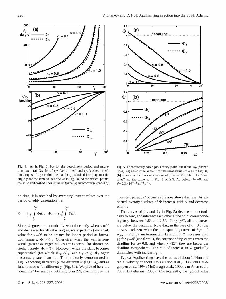
andRf u are defined forα=0.1 only whenγ≤30◦.Figure 4 shows the periods of detachmenttf l and tf u

(Fig. 4a) and the velocitiesCξ l andCξu of the detached ed-dies whose radii areRf l and Rf u (Fig. 4b). Overall, thedetachment period decreases with growingα; however, it in-creases with increasingγ , tending to infinity for the case of

34

incipient basic eddy (BE) centered in E. At the moment t fu , the distance between the two

eddies is

Rfu − Ri( ), which is positive because the incipient BE is less developed.

Therefore, our ABCD contour encloses only the incipient BE.

35

Fig. 3. The theoretical solutions. (a) flR (solid lines) and fuR (dashed lines) plotted against the angle γ. Each pair of intersecting curves is marked by a corresponding value of α. (b)

flR (solid lines), fuR (dashed lines), and iR (dash-and-dotted line) plotted against α. Each pair of divergent curves is marked by a corresponding value of γ. It is seen that the curves corresponding to γ ≥ 450 start from the iR curve. Note that lines depicting flR and

fuR for γ ≥ 300 almost coincide. In both plots: 00 =h , 1111103.2 −−−×= smβ . Intersection of lower and upper boundaries in Fig. 3a defines the critical angle.

Fig. 3. The theoretical solutions.(a) Rf l (solid lines) andRf u

(dashed lines) plotted against the angleγ . Each pair of intersect-ing curves is marked by a corresponding value ofα. (b) Rf l(solidlines),Rf u(dashed lines), andRi (dash-and-dotted line) plottedagainstα. Each pair of divergent curves is marked by a cor-responding value ofγ . It is seen that the curves correspond-ing to γ≥45◦ start from theRi curve. Note that lines depictingRf l and Rf ufor γ≥30◦ almost coincide. In both plots:h0=0,

β=2.3×10−11m−1 s−1. Intersection of lower and upper bound-aries in panel (a) defines the critical angle.

a nearly meridional wall (γ→90◦). This was expected be-cause in this caseCξ→0. Indeed, the curves ofCξ convergemonotonically to zero for each value ofα except 0.1. Inter-section of curves corresponding to lower and upper bound-aries is seen in Fig. 4a; in Fig. 4b, such curves are converg-ing. Therefore, Figs. 3 and 4 suggest that eddy detachmentbecomes restricted whenγ exceeds critical values.

3.2 Mass flux into the eddies

We will now estimate the ratio of the mass flux going intothe rings and the incoming flux (8). Because8 depends



36

37

Fig. 4. As in Fig. 3, but for the detachment period and migration rate. (a) Graphs of flt (solid

lines) and t fu (dashed lines). (b) Graphs of lCξ (solid lines) and uCξ (dashed lines)

against the angle γ for the same values of α as in Fig. 3a. At the critical points, the solid and dashed lines intersect (Fig. 4a) and converge (Fig. 4b).

Fig. 4. As in Fig. 3, but for the detachment period and migra-tion rate. (a) Graphs oftf l (solid lines) andtf u(dashed lines).(b) Graphs ofCξ l (solid lines) andCξ u (dashed lines) against theangleγ for the same values ofα as in Fig. 3a. At the critical points,the solid and dashed lines intersect (panel a) and converge (panel b).

on time, it is obtained by averaging instant values over theperiod of eddy generation, i.e.

8l = t−1f l

tf l∫0

8dt, 8u = t−1f u

tf u∫0

8dt.

Since8 grows monotonically with time only whenγ=0◦

and decreases for all other angles, we expect the (averaged)value for γ=0◦ to be greater for longer period of forma-tion, namely,8u>8l . Otherwise, when the wall is non-zonal, greater averaged values are expected for shorter pe-riods, namely,8u<8l . However, when the slant becomessupercritical (for whichRf u<Rf l and tf u<tf l), 8u againbecomes greater than8l . This is clearly demonstrated inFig. 5 showing8 versusγ for differentα (Fig. 5a), and asfunctions ofα for differentγ (Fig. 5b). We plotted here the“deadline” by analogy with Fig. 5 in ZN, meaning that the

38

39

Fig. 5. Theoretically based plots of lΦ (solid lines) and uΦ (dashed lines): (a) against the angle γ

for the same values of α as in Fig. 3a; (b) against α for the same values of γ as in Fig. 3b. The “dead lines” are the same as in Fig. 5 of ZN. As before, 00 =h , and

1111103.2 −−−×= smβ .

Fig. 5. Theoretically based plots of8l (solid lines) and8u (dashedlines): (a) against the angleγ for the same values ofα as in Fig. 3a;(b) againstα for the same values ofγ as in Fig. 3b. The “deadlines” are the same as in Fig. 5 of ZN. As before,h0=0, andβ=2.3×10−11m−1 s−1.

“vorticity paradox” occurs in the area above this line. As ex-pected, averaged values of8 increase withα and decreasewith γ .

The curves of8u and8l in Fig. 5a decrease monotoni-cally to zero, and intersect each other at the point correspond-ing to γ between 1.5◦ and 2.5◦. For γ≥6◦, all the curvesare below the deadline. Note that, in the case ofα=0.1, thecurves reach zero when the corresponding curves ofRf l andRf u in Fig. 3a are terminated. In Fig. 5b,8 increases withγ ; for γ=0◦(zonal wall), the corresponding curves cross thedeadline forα≈0.8, and whenγ≥15◦, they are below thedeadline everywhere. The rate of increase in8 graduallydiminishes with increasingγ .

Typical Agulhas rings have the radius of about 140 km andradial velocity of about 1 m/s (Olson et al., 1985; van Balle-gooyen et al., 1994; McDonagh et al., 1999; van Aken et al.,2003; Lutjeharms, 2006). Consequently, the typical value



of α for the AC is about 0.08. Accordingly, Fig. 5b sug-gest that8 is roughly 0.16 forγ=0 and 0.035 forγ=20◦,meaning a transport of 11.2 and 2.45 Sv per year. (Equiva-lently, if 5 rings are shed, the transport is 2.24 and 0.49 Svper ring, respectively.) This is consistent with estimates ofvolume fluxes between 0.4 and 3.0 Sv per ring (de Ruijter etal., 1999).

3.3 Varyingh0 andβ

As mentioned, the influence of increasingh0 on the eddyradii is not significant. When we useh0=300 m instead ofzero, the decrease inRf l andRf u with γ becomes slightlymore rapid. In the caseα>0.1, the values (forγ=0◦) areabout 10% less than in Fig. 3a; they are between 170 and175 km, whenγ→90◦. The 300 m thickness values ofRf l

and Rf u at the point of termination forα=0.1 are nearly245 km (instead of 295 km forh0=0). Increasingh0 in-creases the period of eddy generation. The increase intf l

andtf u with increasingγ occurs slower, and forh0=300 m,the periods are reduced by 10% forγ=0◦ and by 60% forγ=60◦ (Fig. 4a). Finally, the influence ofh0 on the averagedvalues of8, as well as on the velocities of detached eddies,is marginal.

Increasingβ leads to quantitative changes. When we useits magnified value (i.e. 6×10−11 m−1 s−1), the final eddy ra-dius is reduced by about 20%. The detachment periods arereduced by approximately 60%. The reduction in8 does notexceed 10%, and the velocity of the detached eddies roughlydouble. Despite the reduction, the final radii are still greaterthan the typical observational values (see ZN, Sect. 1), un-less the potential vorticity (PV) is very small (i.e.α is nearlyone). For example, whenγ=15◦ andα=0.15, thenRf l andRf u are both approximately 256 km, but they change to 144and 146 km, respectively, whenα increases to unity. At thesame time,tf l and tf u change from 82 to 10 and 11 days,respectively. Therefore, when the eddies PV is nearly zero,the magnified value ofβ gives noticeably reduced values forthe detachment period, which naturally is 60–90 days (Byrneet al., 1995; Schouten et al., 2000).

4 Numerical model simulations

4.1 The numerical model

We used the Bleck and Boudra (1986) reduced gravity isopy-cnic model, the description of which was presented in ZN.Here we comment only on the simulation of the detached ed-dies. We initialized the retroflection from a point along thewall that was about 300 km north of the termination of thecontinent. Our modeled time was long (about 210 days) soeven when the eddies’ PV was initially small, it was ulti-mately altered significantly by the cumulative effects of fric-tion during the experiment. Therefore, in our quantitative

comparisons, we always obtained data for nonzero PV andaveraged the values ofα over time.

4.2 Varying the slant

To accelerate the detachment of the rings and make our runsmore economical we chose the magnified value ofβ formost of our experiments. In the experiments with a naturalβ, the period of detachment usually exceeded 200 days butqualitative differences in the evolution of the BE, caused bychangingβ, were not noted.

(i) Zonal coastline: As mentioned, in the case of zonalincoming current, we were obliged to take a high value forthe viscosity coefficient. Although we fixed the parametersso that we can plot the thicknesses every ten days, thestarting value ofα=1 had already approached 0.4 by thetime of fixing the parameters for the first plot. At thatpoint, we identified a chain of four eddies that begun tomove along the wall. During the simulation time, thefirst three eddies quickly weakened, but the fourth kept itsintensity. At the same time, the latter gradually changed thedirection of its movement and shifted away from the wall.Fortunately, we were able to approach the situation when8 was almost unity; in this case, nearly all the incomingmass flux contributed to eddy formation. When we startedwith smaller values ofα, we also obtained weakening andseparation of some eddies, although these effects were notthat pronounced.

(ii) Sub-critical slant: The calculations forγ=15◦ re-quired a relatively large viscosity coefficient of 1000 m2 s−1.(This is typical for numerous published eddy experimentsusing the Bleck and Boudra model.) Forh0=0, we obtainedthe detachment of two eddies, which formed a chain down-stream (Fig. 6). Before the chain formation, however, thefirst detached eddy was absorbed by a second one that camefrom behind and propagated faster. This was followed bythe splitting of the merged eddies into two.

We will see later that the re-absorption of the first eddyoccurs whenγ is large. However, in those cases, the re-absorption ultimately results in a return of the first eddyinto the retroflection area. For smallγ , the occasional re-capturing and splitting of eddies in the model was also foundin the ocean (Goni et al., 1997). Hence, in our simulations,the process may either be real, or an effect of the large viscos-ity coefficient. To check this further, we prolonged the cal-culation so that the modeled time reached 700 days. Interest-ingly, we found that the occasional re-capturing and splittingof eddies continued. Despite the increased viscosity, the firsttwo eddies ultimately left the generation area, and a chain offive eddies was displayed behind.

For h0=300 m, we obtained a somewhat differentsituation. The detached eddies formed a chain with nore-capturing; however, while the first eddy was intense, the



40

Fig. 6. Thickness contours of the numerical simulation for the first 600 days. A chain of eddies is

formed despite intermittent cases of eddies recapturing. Numerical values: 015=γ ,

1=α , 00 =h , and 121000 −= smν . Spacing between contours represents increments of 200 meters, and the maximal thickness of the upper layer is given in meters. The x and y scales are in kilometers. Note that we used 1111106 −−−×= smβ here and in all the following figures.

Fig. 6. Thickness contours of the numerical simulation for the first 600 days. A chain of eddies is formed despite intermittent cases of eddiesrecapturing. Numerical values:γ=15◦, α=1, h0=0, andν=1000 m2 s−1. Spacing between contours represents increments of 200 m, andthe maximal thickness of the upper layer is given in meters. Thex andy scales are in kilometers. Note that we usedβ=6×10−11m−1 s−1

here and in all the following figures.

remaining eddies behind were significantly weaker. Similareffects can be seen for lower starting values ofα, but thetime of eddy development is, as expected, longer.

(iii) Near-critical slant: In contrast to the theoreticalcalculations, simulations usingγ=30◦ andγ=45◦ producededdies that propagated more freely than those in the caseof γ=15◦. One possible explanation lies in our use of thelower viscosity coefficient of 700 m2 s−1in the first case.The radius of the first detached eddy increased only in our

simulation forγ=30◦, α=0.1, andh0=300 m, which couldbe an effect of the long period of detachment. In all othercases, the radii clearly decreased. This could be one of themain factors responsible for maintaining the distances be-tween the rings and protecting them from re-absorption. It isdifficult to say whether this was a consequence of vanishingpossible (theoretical) range of the final radius, frictionalforces, or both. In any case, we conclude that the possibilityof an eddy chain formation for such slants is questionable.For a prolonged numerical simulation, the frequency of ring



41

Fig. 7. The same as Fig. 6, but for 060=γ , 1=α , 00 =h , and 12700 −= smν . The initially

detached eddy is re-captured by the incipient meander. The merged eddies then detach but are recaptured again later; this process repeated itself 3-4 times. The eddy shown in day 600 was later re-captured by day 700 but this recapturing is not displayed in the figure.

Fig. 7. The same as Fig. 6, but forγ=60◦, α=1, h0=0, andν=700 m2 s−1. The initially detached eddy is re-captured by the incipientmeander. The merged eddies then detach but are re-captured again later; this process repeated itself 3–4 times. The eddy shown in day 600was later re-captured by day 700 but this recapturing is not displayed in the figure.

re-capturing increased with time; as a result, after 700 daysof simulation, only two rings propagated around the cape.

(iv) Super-critical slant: Simulations with a slant of60◦, 75◦, and 90◦ clearly confirmed the super-criticality. Insome cases, such as that ofγ=60◦, α=1, andh0=300 m,we did not see a detachment at all. Instead, a meanderof relatively high, but variable, intensity appeared. Othersimulations usingγ=75◦, α=1, andh0=0, showed almost acomplete damping of the first eddy, which remained station-ary after its detachment. The most typical situation is shown

in Fig. 7 (for γ=60◦, α=1, andh0=0). After detachment,the first eddy gradually decayed before being recaptured bythe meandering retroflected current behind. We note thatsuch a scenario is similar to the behavior of rings detachedfrom the retroflection of the EAC, described by Nilsson andCresswell (1981), and Sokolov and Rintoul (2000). We cansay, therefore, that, starting fromγ=60◦, the formation of astable chain of eddies becomes impossible. To confirm this,we further extended our simulations, so that the modeledtime reached 700 days. As a result, the absorbing meanderof the retroflecting current was transformed into an eddy



42

43

44

Fig. 8. Comparison of modeled radii with the numerics. The modeled values of R fl and R fu are plotted against α for h0 = 0 (solid and dashed lines, respectively) and for h0 = 300m (dash-and-dotted and dotted lines, respectively). The numerical values of R correspond to α averaged over the time of the experiments (diamonds for h0 = 0 and circles for

h0 = 300m). Here: (a) 00=γ , and the theoretical curves start from α = 0.1; (b) 030=γ ; (c) 060=γ . The theoretical curves start from the points at which R fl = Ri or R fu = Ri . The curves of R fl and R fu are overlapping in Figs. 8b and 8c because the angle of 300 is

near-critical and 600 is supercritical.

Fig. 8. Comparison of modeled radii with the numerics. The mod-eled values ofRf l andRf u are plotted againstα for h0=0 (solidand dashed lines, respectively) and forh0=300 m (dash-and-dottedand dotted lines, respectively). The numerical values ofR corre-spond toα averaged over the time of the experiments (diamonds forh0=0 and circles forh0=300 m). Here:(a) γ=0◦, and the theo-retical curves start fromα=0.1; (b) γ=30◦; (c) γ=60◦. The theo-retical curves start from the points at whichRf l=Ri or Rf u=Ri .The curves ofRf l andRf u are overlapping in panels (b) and (c)because the angle of 30◦ is near-critical and 60◦ is supercritical.

that was shed. However, later on, it was re-captured by themeander, just as the first detached eddy was. Such a processof shedding and re-capturing was repeating, and no eddiesleft the retroflection area. (The eddy shown in Fig. 7 for

day 600 was later re-captured by day 700.) In view of this,we suggest that, for such values of the slant, re-capturingbecomes systematic and overwhelms the formation of thechain of eddies.

We should comment here about the situation whenα issmall. Our simulations withα=0.1 andγ=60◦ and 75◦ qual-itatively confirmed our theoretical prediction that the eddycannot grow because theβ-induced force initially exceedsthe combined force of the currents (i.e. their long-shore mo-mentum flux). In such cases, the plots showed the formationof a meander that was gradually forced into the wall. Its lon-gitudinal dimension, along the wall, became much greaterthan the transverse one, negating our assumption of a nearlycircular form. Eventually, an eddy of a smaller radius wasformed from this meander. Further, the formed eddy con-tinued decaying and exhibited almost no movement. We ex-pected that it would finally be reabsorbed, but we did notreach that state.

4.3 Simulation-theory comparison

In addition to the qualitative analysis of ring behavior dis-cussed above, we carried out a detailed comparison of thetheoretical modeling and the numerical simulations. (For thispurpose, we used the magnified value ofβ.) We comparedthe eddy radius at the moment of detachment,Rf , the eddypropagation velocity (Cξ ), and the ratio of the mass flux go-ing into the eddies and the incoming flux (8).

Two introductory comments should be made here. First,Nof and Pichevin (2001, NP, hereafter) carried out the quan-titative comparison of the ratioq/Q as a function of time,whereq is outgoing mass flux. In their case, it was veryimportant to take into account the time evolution of the pa-rameterα, which was dramatically altered by the viscosityin the numerics. For us, it was inconvenient to conduct asimilar analysis because8 was also variable in time, and wewere operating mainly with its time-averaged values. There-fore, we simplified our analysis by assuming that the value of8, averaged over the time of the numerical experiment, cor-responded to the value ofα averaged in the same way, andso did with the other parameters that we considered. Sec-ond, we also averaged the value ofCξ . Wherever possible,we used an averaging period between the moment of detach-ment and the last step in our experiment. However, in mostsimulations with supercritical values ofγ , we were obligedto use a period between the detachment and the re-absorptionof the eddy.

According to NP, the coefficientα decreases quickly whenits initial value is unity (zero PV). In the case of finite PVoutflow, α decreases more slowly. However, in most of theexperiments that started withα=0.1, we observed a slightgrowth inα, especially for largeγ . Most likely, this was aconsequence of a decrease in the size of the meander/eddydue toβ. Resulting from the above-mentioned behaviorsof α, its average value accumulated in relatively narrow



intervals: between 0.12 and 0.36 forh0=0, and between 0.08and 0.33 forh0=300 m.

Figure 8 shows a comparison ofRf in the analytics andnumerical simulations. Bearing in mind that the starting val-ues ofα in the numerics were 1, 0.4, and 0.1, we mark thenumerical results for the time-averaged values ofα with cir-cles and diamonds. Analyzing Fig. 8a, b, and c, whereγ

is 0◦, 30◦ and 60◦ (respectively), we see that the numericalsimulations confirm the theoretical tendency for the radius todecrease with growing angle. However, such a decrease isweaker than in the theoretical prediction. In this connection,the scattering inRf weakens withγ . Strictly speaking, ourtheory does not allow us to estimateRf corresponding ex-actly to theα obtained in the numerics whenγ is large, be-cause under such conditions, the BE is forced into the wall.We conclude that, for nonzeroγ , the numerical radii calcula-tions give larger values than our theoretical model (by about20–30%) probably due to friction which caused the eddies toflatten out. In the case of a zonal wall, the agreement is betteroverall, but the scattering of numerical values is significant.

Figure 9 shows a comparison of the theoretical and nu-merical values ofCξ for γ=0◦, 30◦, and 60◦, whereas Fig. 10shows the comparison of8 for the same angles. (We notethat there are two circles instead of three in the lower panelof Fig. 9. This is because, as mentioned, in our simulationwith γ=60◦, α=1 andh0=300 m we did not achieve detach-ment, so we could not compute the eddy drift velocity.) Theagreement ofCξ is poor forγ=0, which could be a result ofvery large viscosity in our numerics, leading to strong decel-eration of eddies. This agreement improves with growingγ

for h0=0; in the case ofh0=300 m it is worse because ofthe noticeable scattering in the numerical values. Neverthe-less, we can suggest that Fig. 9 confirms Eq. (3), which wasintroduced without any rigorous analysis.

The agreement seems to be not very good with regard to8, especially for nonzeroγ . However, it is not easy to com-pute the mass flux numerically because of noise (e.g. in theform of Kelvin waves and secondary meandering of the out-going flow, and frictional effects) leading to ambiguity in theboundaries of this flux. The scattering of the numerical val-ues ranges between slightly negative and about 0.18, which isadmissible when the theoretical values are between zero and0.2 (forγ=30◦), or even between zero and 0.05 (forγ=60◦).In either case, the numerics clearly confirm that8 is consid-erably smaller when the coastline is slanted.

5 Summary and conclusions

The main aim of our theoretical and numerical analyses wasto examine the hypothesis that the glacial AC was similarto the present day EAC where, due to the orientation of thecoastline, no mean rings shedding is usually observed. Ac-cording to our hypothesis, the shedding of eddies is severelyrestricted when the slant angleγ is about 65◦ (the present

45

46

47

Fig. 9. As in Fig. 8 except that this is a comparison of the modeled propagation rates with the numerics.

Fig. 9. As in Fig. 8 except that this is a comparison of the modeledpropagation rates with the numerics.

EAC, and the glacial AC) and greater, but occurs steadilywhenγ is smaller than about 20◦ (present AC).

To examine this hypothesis we developed a non-linearmodel of retroflecting currents that flow along slanted coast-lines. We studied the dependence of ring diameter, speed andfrequency of shedding, on the coastline slant, the PV of theformed eddies, and the thickness of the surrounding upperlayer. The results are shown in Figs. 3–5. We treated the an-gle of visible intersection of the lower and upper boundariesof the theoretical eddy radius (Fig. 3) as the critical angle.Indeed, according to our definition of the lower boundary(osculating rings), the convergence of the lower and upper



48

49

50

Fig. 10. As in Fig. 8 except that we show here a comparison of the mass flux ratio (Φ). Fig. 10. As in Fig. 8 except that we show here a comparison of themass flux ratio (8).

boundaries means that only a chain of “kissing” detachedrings can form downstream. This implies that, in practice, therings are likely to hinder each other owing, for instance, toviscosity. Because for supercritical slants, small long-shoredrift speeds are predicted for detached rings, the slowly mov-ing eddy will be hindered and re-captured by the one behindit or by a meander of the retroflected current. Such a scenarioagrees well with the dynamics of the EAC rings describedby Nilsson and Cresswell (1981), and Sokolov and Rintoul(2000). These rings usually stay at the same place for a longtime and may eventually re-coalesce with the EAC.

We used a modified version of the Bleck and Boudra(1986) reduced gravity isopycnic model and obtained plotssurprisingly similar to the observed EAC dynamics when theslant was taken to be 60◦ or more (Fig. 7). Also, as expected,we obtained chains of detached eddies when the slant was15◦ (Fig. 6) and, a less clear chain whenγ=30◦. The tran-sition range of slant angles was between 25◦ and 50◦, whichagrees with our description of the critical angle that is ap-proximately 18◦, 25◦, 33◦, and 40◦ whenα is 0.1, 0.2, 0.5,and unity (respectively). During most of our simulation,α

was between 0.15 and 0.3 and the variables obtained in thetheoretical modeling were in satisfactory quantitative agree-ment with our numerical simulations (Figs. 8–10). On thisbasis, we suggest that the significant reduction in the ex-change between the Indian and South Atlantic Oceans duringthe glacials and the YD was due to a northward migration ofthe WSC. This led the AC retroflection area to shift to a lati-tude of a supercritical coastal slant (Fig. 1). Other importantresults of our study can be summarized as follows:

– An increase inγ leads to a decrease in the radii of de-tached rings and makes them less sensitive to variationsin α (Fig. 3). Nevertheless, even in the case of supercrit-ical slant, the theoretical values ofRf are 185–220 kmand, therefore, still noticeably greater than the observa-tional values.

– The mass-flux ratio8 decreases monotonically with in-creasing coastal slant (Fig. 5). Whenγ≥6◦, it becomesless than unity (even for eddies with zero PV, i.e. intenseeddies) implying that the “vorticity paradox” discussedby ZN is circumvented.

– Our assumption of a nearly circular BE fails when thePV is large (weak eddies) andγ is not very small. Inthat case, the BE does not grow; rather, it is forced intothe wall and deforms.

Concerning the distance between two consecutive eddies, wenote that the ratioRf u/Rf l is maximal in the case of zonalwall, when it is approximately 1.06 (i.e. less than 21/5).Therefore, we conclude that, theoretically, the separation dis-tance should not exceed the eddy diameter. This conclusionis not far from the observational data, even though the eddydiameter is smaller than our theory yields. Indeed, if the ed-dies are shed on average 5 times per year, and their migrationrate varies between 2 and 10 cm/s, then, during the period ofgeneration, the eddy migrates 380 km on average, and at themost 630 km. Taking into account a typical eddy radius of140 km, we obtain that the ratio(d/2R) is 0.36 in average,with a maximal value of 1.25.

As is frequently the case, our ability to compare our the-oretical results with the numerical simulations was limiteddue to the effect of viscosity in the numerics, which led toa relatively narrow range ofα. In addition, the viscosity inthe numerics makes the outgoing flux blurry, resulting in a



possibility of errors as large as 0.2 in the determination of8. Despite both of these aspects, our comparison is use-ful. Although in our numerical simulations we confirmedthe observation that re-capturing and re-splitting of eddiescan be a possible cause of non-regularity in their shedding(Goni et al., 1997), we find that non-regularity could also beconnected with variability of the retroflection position (Lut-jeharms, 2006). For example, we note that Esper et al. (2004)pointed out seasonality of its position.

Our results also agree with Chassignet and Boudra’s(1988) sensitivity analysis, which showed that decreasingcoastal slant leads to an increase in the production of rings.On the other hand, the numerical experiments by Pichevin etal. (1999) showed that the dependence of the periodicity ofrings shedding on the slant angle could be negligible. Thismight be a result of the specific geometry of coastline in theirmodel. We leave this issue as a subject for future investiga-tions. Finally, we note that taking into account the coastlineslant could also improve understanding of other retroflectingoceanic currents such as the North Brazil Current (NBC).Unfortunately, the question of a priori determination of theeddy PV remains unanswered, and this is significant partic-ularly when the vorticity of the incoming fluid is cyclonicrather than anticyclonic.

Appendix A

List of symbols

AAIW Antarctic Intermediate WaterAC Agulhas CurrentBE basic eddyCx eddy velocity in the open oceanCξ eddy migration rate along the slanted coastCξf eddy migration rate after detachmentCξ l, Cξu values of Cξf for eddies with radii

Rf l, Rf u, respectivelyd distance between consecutive eddiesdu “upper” boundary ofdEAC East Australian Currentg′ reduced gravityh0 upper layer thickness at the wallH upper layer thickness outside the retroflec-

tion areaHf l, Hf u values ofH at the momentstf l, tf u, re-

spectivelyLGM Last Glacial MaximumMOC meridional overturning circulationNADW North Atlantic Deep WaterNP Nof and Pichevin (2001)

PSU practical salinity unitsPV potential vorticityQ mass flux of the incoming currentQR volume flux of the ringsq mass flux of the retroflected currentR radius of the eddy (a function of time)Ri initial radius of the eddyRf radius of detached eddyRf l, Rf u “lower” and “upper” boundaries ofRf

S salinitySA Southern AtlanticSEA Southeastern Atlantict timetf period of the eddies generationtf l, tf u “lower” and “upper” boundaries oftfWSC wind stress curlYD Younger DryasZN Zharkov and Nof (2008)α vorticity (twice the Rossby number)β meridional gradient of the Coriolis param-

eterγ slant of coastlineξ ,η axes of rotated moving coordinate system8 ratio of mass flux going into the eddies and

incoming mass flux8l, 8u values of 8 for eddies with radii

Rf l, Rf u, respectively.

Acknowledgements.The study was supported by the NASAunder the Earth System Science Fellowship Grant NNG05GP65H.V. Zharkov was also funded by the Jim and Shelia O’BrienGraduate Fellowship. Nof acknowledges a detailed and extensiveemail exchange with Arnold Gordon regarding the salt balance cal-culation described in Sect. 1.2. We are grateful to Steve van Gorderfor helping in the numerical simulations, to Donna Samaan forhelping in preparation of manuscript, and to Joanna Beall forhelping in improving the style.

Edited by: A. Sterl

References

Andrews, J. C. and Scully-Power, P.: The structure of an East Aus-tralian Current anticyclonic eddy, J. Phys. Oceanogr., 6, 756–765, 1976.

Arruda, W. Z., Nof, D., and O’Brien, J. J.: Does the Ulleung eddyowe its existence toβ and nonlinearities?, Deep-Sea Res., 51,2073–2090, 2004.

Bard, E.: Climate shock: abrupt changes over millennial timescales, Phys. Today, 55, 32–38, 2002.

Berger, W. H. and Wefer, G.: Expeditions into the past: paleo-ceanographic studies in the South Atlantic, pp. 35–156, Springer-Verlag, Berlin-Heidelberg, 1996.

Bleck, R. and Boudra, D.: Wind-driven spin-up in eddy resolvingocean models formulated in isopycnic and isobaric coordinates,J. Geophys. Res., 91, 7611–7621, 1986.



Bostock, H. C., Opdyke, B. N., Gagan, M. K., Kiss, A. E., andFifield, L. K.: Glacial/interglacial changes in the East Australiancurrent, Clim. Dynam., 26, 645–659, 2006.

Byrne, A. D., Gordon, A. L., and Haxby, W. F.: Agulhas eddies:A synoptic view using geosat ERM data, J. Phys. Oceanogr., 25,902–917, 1995.

Chassignet, E. P. and Boudra, D. B.: Dynamics of the Agulhasretroflection and ring formation in a numerical model. II. En-ergetics and ring formation, J. Phys. Oceanogr., 18, 304–319,1988.

de Ruijter, W. P. M.: Asymptotic analysis of the Agulhas and BrazilCurrent systems, J. Phys. Oceanogr., 12, 361–373, 1982.

de Ruijter, W. P. M., Biastoch, A., Drijfhout, S. S., Lutjeharms, J.R. E., Matano, R. P., Pichevin, T., van Leeuwen, P. J., and Weijer,W.: Indian-Atlantic interocean exchange: Dynamics, estimationand impact, J. Geophys. Res., 104, 20 885–20 910, 1999.

Esper, O., Versteegh, G. J. M., Zonneveld, K. A. F., and Willems,H.: A palynological reconstruction of the Agulhas Retroflec-tion (South Atlantic Ocean) during the Late Quaternary, GlobalPlanet. Change, 41, 31–62, 2004.

Gasse, F.: Hydrological changes in the African tropics since theLast Glacial Maximum, Quat. Sci. Rev., 19, 189–211, 2000.

Goni, G. J., Garzoli, S. L., Roubicek, A. J., Olson, D. B., andBrown, O. B.: Agulhas ring dynamics from TOPEX/POSEIDONsatellite altimeter data, J. Mar. Res., 55, 861–883, 1997.

Gordon, A. L., Lutjeharms, J. R. E., and Grundlingh, M. L.: Strat-ification and circulation at the Agulhas Retroflection, Deep-SeaRes., 34, 565–599, 1987.

Howard, W. R. and Prell, W. L.: Late quaternary surface circula-tion of the southern Indian Ocean and its relationship to orbitalvariation, Paleoceanogr., 7, 79–117, 1992.

Kawagata, S.: Tasman front shifts and associated paleoceano-graphic changes during the last 250,000 years: foraminiferal ev-idence from the Lord Howe Rise, Mar. Micropal., 41, 167–191,2001.

Knorr, G. and Lohmann, G.: Southern Ocean origin for the resump-tion of the Atlantic overturning circulation during deglaciation,Nature, 424, 532–536, 2003.

Lutjeharms, J. R. E.: The exchange of water between the South In-dian and South Atlantic Oceans, in: The South Atlantic: Presentand Past Circulation, edited by: Wefer, G., Berger, W., andSielder, G., pp. 125–162. Springer-Verlag, Berlin-Heidelberg,1996.

Lutjeharms, J. R. E.: The Agulhas Current, Springer-Verlag, Berlin-Heidelberg-New York, XIV, 330 p., 2006.

Martinez, J. I.: Late Pleistocene palaeoceanography of the TasmanSea: implications for the dynamics of the warm pool in the west-ern Pacific, Palaeogreogr. Palaeoclimatol. Palaeoecol., 112, 19–62, 1994.

Martinez, J. I., de Deckker P., and Barrows, T. T.: Palaeoceanog-raphy of the western Pacific warm pool during the last glacialmaximum: long-term climatic monitoring of the maritime conti-nent, in: Bridging Wallace’s line, edited by: Kershaw, P., Bruno,D., Tapper, N., Penny, D., and Brown, J., Adv. Geoecol., 34,147–172, 2002.

McDonagh, E. L., Heywood, K. J., and Meredith, M. P.: On thestructure, paths, and fluxes associated with Agulhas rings, J.Geophys. Res., 104, 21 007–21 020, 1999.

Nilsson, C. S., Andrews, J. C., and Scully-Power, P.: Observation

of eddy formation off East Australia, J. Phys. Oceanogr., 7, 659–669, 1977.

Nilsson, C. S. and Cresswell, G. R.: The formation and evolutionof East Australian Current warm-core eddies, Progr. Oceanogr.,9, 133–183, 1981.

Nof, D.: On the migration of isolated eddies with application toGulf Stream rings, J. Mar. Res., 41, 399–425, 1983.

Nof, D.: The momentum imbalance paradox revisited, J. Phys.Oceanogr., 35, 1928–1939, 2005.

Nof, D. and Pichevin, T.: The ballooning of outflows, J. Phys.Oceanogr., 31, 3045–3058, 2001.

Nof, D. and Van Gorder, S.: Did an open Panama Isthmus Corre-spond to an invasion of Pacific water into the Atlantic?, J. Phys.Oceanogr., 33, 1324–1336, 2003.

Olson, D. B. and Evans, R. H.: Rings of the Agulhas Current, Deep-Sea Res., 33, 27–42, 1986.

Peeters, F. J. C., Acheson, R., Brummer, G.-J. A., de Ruijter, W. P.M., Schneider, R. R., Ganssen, G. M., Ufkes, E., and Kroon, D.:Vigorous exchange between the Indian and Atlantic oceans at theend of the past five glacial periods, Nature, 430, 661–665, 2004.

Pichevin, T., Nof, D., and Lutjeharms, J. R. E.: Why are there Ag-ulhas Rings?, J. Phys. Oceanogr., 29, 693–707, 1999.

Rau, A. J., Rogers, J. Lutjeharms, J. R. E., Giraudeau, J., Lee-Thorp, J. A., Chen, M.-T., and Waelbroeck, C.: A 450-kyr recordof hydrological conditions on the western Agulhas Bank Slope,south of Africa, Mar. Geol., 180, 183–201, 2002.

Sandal, C. and Nof. D.: A new analytical model for Heinrich eventsand climate instability, J. Phys. Oceanogr., 38, 451–466, 2008.

Schouten, M. W., de Ruijter, W. P. M., van Leeuwen, P. J., andLutjeharms, J. R. E.: Translation, decay and splitting of Agulhasrings in the south-eastern Atlantic ocean, J. Geophys. Res., 105,21 913–21 925, 2000.

Schouten, M. W., de Ruijter, W. P. M., and van Leeuwen, P. J.:Upstream control of the Agulhas ring shedding, J. Geophys. Res.,107, doi:10.1029/2001JC000804, 2002.

Shi, C. and Nof, D.: The destruction of lenses and generation ofwodons, J. Phys. Oceanogr., 24, 1120–1136, 1994.

Sokolov, S. and Rintoul, S.: Circulation and water masses of thesouthwest Pacific: WOCE Section P11, Papua New Guinea toTasmania, J. Mar. Res., 58, 223–268, 2000.

Speich, S., Lutjeharms, J. R. E., Penven, P., and Blanke, B.: Roleof bathymetry in Agulhas Current configuration and behavior,Geophys. Res. Lett., 33, L23611, doi:10.1029/2006GL027157,2006.

Tilburg, C. E., Hulburt, H. E., O’Brien, J. J., and Shriver, J. F.:The dynamics of the East Australian current system: the Tasmanfront, the east Auckland current and the East Cape current, J.Phys. Oceanogr., 31, 2917–2943, 2001.

van Aken, H. M., van Veldhoven, A. K., Veth, C., de Ruijter, W.P. M., van Leeuwen, P. J., Drijfhout, S. S., Whittle, C. P., andRouault, M.: Observations of a young Agulhas ring, Astrid, dur-ing MARE in March 2000, Deep-Sea Res., 50, 167–195, 2003.

van Ballegooyen, R. C., Grundlingh, M. L., and Lutjeharms, J. R.E.: Eddy fluxes of heat and salt from the southwest Indian Oceaninto the southeast Atlantic Ocean: A case study, J. Geophys.Res., 99, 14 053–14 070, 1994.

Weijer, W., de Ruijter, W. P. M., Dijkstra, H. A., and van Leeuwen,P. J.: Impact of interbasin exchange on the Atlantic OverturningCirculation., J. Phys. Oceanogr., 29, 2266–2284, 1999.



Weijer, W., De Ruijter, W. P. M., and Dijkstra, H. A.: Stability of theAtlantic overturning circulation: Competition between BeringStrait freshwater flux and Agulhas heat and salt sources, J. Phys.Oceanogr., 31, 2385–2402, 2001.

Zharkov, V. and Nof, D.: Retroflection from slanted coastlines –circumventing the “vorticity paradox”, Ocean Sci. Discuss., 5,1–37, 2008,http://www.ocean-sci-discuss.net/5/1/2008/.


http://www.ocean-sci-discuss.net/5/1/2008/

agulhas ring injection into the south atlantic during glacials and

Documents