Ea

M

a

b

c

a

ARAA

KASOHA

1

atplga

tun2go2dp

0d

Agricultural Water Management 109 (2012) 81– 93

Contents lists available at SciVerse ScienceDirect

Agricultural Water Management

j ourna l ho me page: www.elsev ier .com/ locate /agwat

valuation of subsurface drip irrigation design and management parameters forlfalfa

aziar M. Kandelousa,∗, Tamir Kamaia, Jasper A. Vrugtb, Jirí Simunekc, Blaine Hansona, Jan W. Hopmansa

Department of Land, Air and Water Resources, University of California, Davis, CA 95616, USADepartment of Civil and Environmental Engineering, University of California, Irvine, CA 92697, USADepartment of Environmental Science, University of California Riverside, CA 92521, USA

r t i c l e i n f o

rticle history:eceived 19 September 2011ccepted 26 February 2012vailable online 17 March 2012

eywords:lfalfaubsurface drip irrigation

a b s t r a c t

Alfalfa is one of the most cultivated crops in the US, and is being used as livestock feed for the dairy, beef,and horse industries. About nine percent of that is grown in California, yet there is an increasing concernabout the large amounts of irrigation water required to attain maximum yield. We introduce a conceptualframework to assist in the design and management of subsurface drip irrigation systems for alfalfa thatmaximize yield, while minimizing deep percolation water losses to groundwater. Our approach combinesthe strengths of numerical modeling using HYDRUS-2D with nonlinear optimization using AMALGAMand Pareto front analysis. The HYDRUS-2D model is used to simulate spatial and temporal distributions of

ptimizationYDRUS-2DMALGAM

soil moisture content, root water uptake, and deep drainage in response to drip-line installation depth anddistance, emitter discharge, irrigation duration and frequency. This model is coupled with the AMALGAMoptimization algorithm to explore tradeoffs between water application, irrigation system parameters, andcrop transpiration (Ta), to evaluate best management practices for subsurface drip irrigation systems inalfalfa. Through analysis of various examples, we provide a framework that seeks optimal design andmanagement practices for different root distribution and soil textures.

. Introduction

Alfalfa is one of the most widely cultivated crops in the world,nd is used as livestock feed for the dairy, beef, and horse indus-ries (Breazeale et al., 2000). The United States is the world’s largestroducer of alfalfa, with an annual value of about one billion dol-

ars. About nine percent of all alfalfa produced in the United States isrown in California, with an average acreage of 360,000 ha (900,000cres, Alfalfa’s commodity fact sheet, 2011).

Because of California’s semi-arid climate, irrigation is necessaryo attain high yields. In California, about 1.2 billion m3 of water issed to irrigate alfalfa each year, which is about 20% of Califor-ia’s developed water supply (Natural Resources Defense Council,001; Putnam et al., 2001). These large amounts of required irri-ation water have encouraged the development and applicationf efficient irrigation systems. Hutmacher et al. (2001) reported a

0% increase in water use efficiency for alfalfa by using subsurfacerip irrigation (SDI) rather than furrow irrigation. Another com-arison between SDI and flood irrigation by Godoy et al. (2003)

∗ Corresponding author.E-mail address: mkandelous@ucdavis.edu (M.M. Kandelous).

378-3774/$ – see front matter. Published by Elsevier B.V.oi:10.1016/j.agwat.2012.02.009

Published by Elsevier B.V.

demonstrated that subsurface irrigation significantly improved theyield by about 25%, while using about 40% less water than flood irri-gation. The study by Alam et al. (2002) showed that a well-designedSDI system can potentially decrease the volume of applied waterby about 22%, while increasing the yield by 7%, compared to usinga center pivot sprinkler system.

Alfalfa, a perennial crop, is harvested between 3 and 11 timesthroughout the year, depending on soil, irrigation practice, and cli-matic conditions. One of the biggest challenges in alfalfa productionis the selection of irrigation design and management practices thatmaximize yield (and thus income), while simultaneously minimiz-ing water losses. In addition, at harvesting times the soil surfaceshould be sufficiently dry so that machinery can drive over thefield without creating stressed root zone soil moisture conditions,allowing for quick re-growth of the cut alfalfa. In addition, thenonlinearity of soil–water–plant relationship makes it particularlydifficult to find irrigation systems and strategies that maximizeyield while simultaneously minimizing water losses. For all thesereasons the optimal irrigation system and design practices are not

immediately obvious for most climatic and soil conditions. A sub-surface drip system, however, is ideally suited as it directly supplieswater to the rooting zone at high frequency, allowing control ofsurface soil moisture required, for dry soil surface conditions prior

82 M.M. Kandelous et al. / Agricultural Water Management 109 (2012) 81– 93

Nomenclature

AWmax maximum possible applied water [L3 L−2]D drip-line depth [L]DP deep percolation [L3 L−2]DPmax maximum possible deep percolation [L3 L−2]ETa actual evapotranspiration [LT−1]ETo reference evapotranspiration [LT−1]ETp potential evapotranspiration [LT−1]f irrigation frequency [T−1]FE finite elementsh soil water pressure head [L]h1, h2, h3, and h4 parameters of Feddes uptake reduction

function [L]ID irrigation duration [T]I1 optimization scenario such that

ωD = ωL = ωAW = ωDP = 1I2 optimization scenario such that ωD = 0 and

ωL = ωAW = ωDP = 1I3 optimization scenario such that ωD = ωDP = 0 and

ωL = ωAW = 1ISA irrigation scheduling Alfalfa modelK(h) unsaturated hydraulic conductivity [LT−1]Kc crop coefficientKs saturated hydraulic conductivity [L T−1]L drip-line distance [L]l shape parameter in the van Genuchten soil

hydraulic functions

Lx width of the soil surface associated with transpira-tion [L]

m shape parameter in the van Genuchten soilhydraulic functions, m = 1 − 1/n

N number of irrigation eventsn shape parameter in the van Genuchten soil

hydraulic functionsOFi objective function (i)Q drip-line discharge [L3 L−1 T−1]q drip-line discharge [L3 L−2 T−1]R1 optimization scenario using uniform root distribu-

tionR2 optimization scenario using linear root distributionS(x,z) sink term [L3 L−3 T−1]SDI subsurface drip irrigationSe effective saturationSp potential root water uptake [L3 L−3 T−1]t time [T]T1 optimization scenario using clay-loam soilT2 optimization scenario using loam soilT3 optimization scenario using sandy-loam soil

Ta actual plant transpiration [LT−1]Tp potential plant transpiration [LT−1]x horizontal spatial coordinate [L]z vertical spatial coordinate [L]˛(h) Feddes’ uptake reduction function˛VG shape parameter in the van Genuchten soil

hydraulic functionsˇ(x,z) normalized root density for any coordinate in the

two-dimensional soil domain [L2]� volumetric water content [L3 L−3]�r residual water content [L3 L−3]�s saturated water content [L3 L−3]

root zone area [L2]

ωD, ωL, ωAW, ωDP weighting factors for D, L, AW, and DP inobjective functions

to alfalfa cutting. We use detailed numerical soil water flow mod-eling with HYDRUS-2D (Simunek et al., 2008), combined with amulti-criteria optimization framework to determine optimal irri-gation water management strategies for subsurface drip irrigationof alfalfa.

Past sensitivity analysis (Gärdenäs et al., 2005) has shown thatthe root distribution exerts strong influence on subsurface drip irri-gation design and management practices, as water uptake by plantroots determines spatial and temporal patterns in soil water avail-ability. Whereas various past studies investigated root distributionsof alfalfa (Abdul-Jabbar et al., 1982; Meinzer, 1927), we know of nostudies that evaluate the effects of SDI on alfalfa root distribution.

The ever increasing pace of computational power along withsignificant advances in numerical modeling of soil–plant–waterrelationships enables the application of numerical vadose zonesimulation models for analyses of micro-irrigation systems involv-ing a wide range of crops. The HYDRUS-2D (Simunek et al., 2006,2008) model has been widely used for this purpose, including forSDI (Gärdenäs et al., 2005; Hanson et al., 2006; Skaggs et al., 2006;Hanson et al., 2008). The effect of different irrigation design vari-ables such as drip-line distance and drip-line installation depthcan be readily simulated by such a modeling system for a range ofsoil types. Whereas these design parameters are relevant to wateravailability for crops and soil types, drip-line depth and distancealso have economic consequences as they essentially determineirrigation system costs. Other factors to consider are leachinglosses, rodent damage, and requirement of soil dryness beforeharvesting.

In this study, we present a general purpose multi-criteria opti-mization framework to help in the design of optimal subsurfacedrip irrigation systems for alfalfa. Instead of providing specific irri-gation system and water application recommendations, we presenta flexible optimization tool that allows definition of a range ofobjective functions to be minimized, using multiple criteria andweights. Our approach combines the strengths of numerical vadosezone modeling using HYDRUS-2D with the AMALGAM evolution-ary search (Vrugt and Robinson, 2007) and Pareto front (Wöhlinget al., 2008) algorithms, to provide water application strategiesthat maximize yield and minimize water loss for a range of irri-gation system designs. In particular, we seek to optimize drip-lineinstallation depth and distance, irrigation duration, and irrigationfrequency, while maximizing root water uptake and minimizingirrigation water losses by leaching. In addition, our analysis is espe-cially designed to ensure sufficiently dry soil surfaces at harvestingtimes. These optimal parameters are determined for different rootdistribution (uniform and linear), and soil types (sandy loam, loam,and clay loam). We realize that economics of irrigation system andwater costs should also be considered, however, we do not con-sider these factors in the present analysis, as dollar values can beeasily included in the formulation of the objective functions whenavailable.

2. Materials and methods

A schematic of the followed computational procedures to arriveat the final set of optimal design and decision parameters is shown

in the flow chart of Fig. 1. The main computational loop is defined bythe AMALGAM evolutionary search algorithm (Vrugt and Robinson,2007), selecting specific values of drip-line installation depth (D)and distance (L), irrigation duration (ID) and frequency (f) from

M.M. Kandelous et al. / Agricultural Water Management 109 (2012) 81– 93 83

Start

AMALGAM

Generate

system design and

management

parameters

Irrigation

frequency, f

Drip-line

installation

depth, D

Irrigation

duration, ID Drip-line

distance, L

HYDRUS-2D Calculate OF1

Calculate Ta and DP

Calculate OF2 and OF 3Calculate average soil water

potential in top 30 cm

Less than

threshold?NoPenalize the objective functions

Yes

Convergence? No

Yes

Return Pareto optimal solution

End

F s diago

tnestrftwvUa

Table 1Ranges of system design and water application parameters for HYDRUS model sim-ulations, as defined for AMALGAM search algorithm.

Lower value Upper value Interval

ig. 1. Flow diagram of the presented multi-objective optimization approach. In thibjective function i.

he prior allowed ranges (Table 1). For each of the selected combi-ations, the HYDRUS-2D unsaturated water flow model (Simunekt al., 2008) simulates soil water flow for the specific irrigationystem selected and computes the spatial and temporal distribu-ions of soil water potential and water content, with correspondingoot water uptake, and drainage and actual transpiration ratesor the growing season. In addition, cumulative values of actualranspiration (Ta), deep percolation losses (DP), and average soil

ater pressure head values for the top 30-cm at predefined har-

esting times are computed for each growing season simulation.pon completion of each HYDRUS simulation, AMALGAM evalu-tes the three objective functions (OF’s) of Eqs. (8) or (9) with

ram, Ta denotes actual transpiration, DP is deep percolation, and OFi represents the

Drip-line depth (cm), D 20 70 5Drip-line distance (cm), L 40 300 10Duration of irrigation (h), ID 8 24 1Irrigation frequency (days−1), f 1/7 1 1/7

8 l Wate

cvaIcnpcttowpmctpstamafoatc

2

(aa

2

Ru

wtrtztcttve

S

K

wt[Tdo

4 M.M. Kandelous et al. / Agricultura

orresponding weighting factors (Eq. (8) only), and uses the OF-alues to seek new system design parameters from the priorllowed ranges for a next iteration with HYDRUS-2D calculations.t is here where the AMALGAM search algorithm is novel and effi-ient, in seeking all possible optimal solutions with a minimumumber of HYDRUS-2D simulation iterations required. Upon com-letion of the optimization, as determined by various pre-definedonvergence criteria, AMALGAM derives the Pareto solution sethat consists of a sample of optimal solutions representing differentradeoffs to the multi-criteria optimization problem. For this studyf alfalfa subsurface drip irrigation, the main tradeoffs are betweenater application and transpiration. As an example of these com-lex trade-offs, for large distance between drip-lines more waterust be applied in order to wet the root zone and satisfy non-stress

onditions for high transpiration. However, adding more watero the root zone also increases deep percolation, whereas otherarameters such as drip-line installation depth also influence tran-piration and deep percolation. Thus, we seek a balance betweenhe different processes and parameters. This trade-off balance ischieved by the Pareto front analysis, and provides for develop-ent of optimal subsurface drip irrigation system parameters for

range of soil types (Table 2) and typical root distributions. In theollowing we provide a detailed description of the various elementsf our optimization framework. Although we limit our attention tolfalfa, the methodology presented herein can readily be appliedo develop efficient drip irrigation designs for a wide range ofrops.

.1. Numerical HYDRUS simulations

The two-dimensional module of the HYDRUS-2D/3D packageSimunek et al., 2008) was used to simulate soil water movementnd plant root water uptake for the specific irrigation system designnd water application parameters defined in Table 1.

.1.1. Soil water movementThe HYDRUS-2D model uses the two-dimensional form of

ichards’ equation to describe transient water flow in isotropicnsaturated soils:

∂�

∂t= ∂

∂x

[K(h)

∂h

∂x

]+ ∂

∂z

[K(h)

∂h

∂z+ K(h)

]− S(h) (1)

here � is the soil’s volumetric water content [L3 L−3], h denoteshe soil water pressure head [L], S(h) is a sink term [L3 L−3 T−1]epresenting plant root water uptake, t signifies time [T], K(h) ishe unsaturated hydraulic conductivity function [LT−1], and x and

are the horizontal and vertical spatial coordinates [L], respec-ively, of the simulated soil domain. Solution of Eq. (1) requiresharacterization of the soil hydraulic properties, as defined byhe soil water retention, �(h), and unsaturated hydraulic conduc-ivity function, K(h). We used the constitutive relationships ofan Genuchten-Mualem (van Genuchten, 1980) and represent theffective saturation, Se by:

e = � − �r

�s − �r= 1

(1 + |˛VGh|n)m (2)

and

(h) = KsSle

[1 − (1 − S1/m

e )m]2

, (3)

here �s and �r represent the saturated and residual water con-ent [L3 L−3], respectively, Ks is the saturated hydraulic conductivity

LT−1], ˛VG [L−1], n, and l are shape parameters, and m = 1 − 1/n.hough these four parameters are directly related to pore sizeistribution, pore connectivity and tortuosity, they are generallybtained from fitting of �(h) and K(h) data to functions (2) and

r Management 109 (2012) 81– 93

(3), respectively. Eq. (1) is solved using a Galerkin type linearfinite element method applied to a network of triangular ele-ments. Time integration is achieved using an implicit (backwards)finite difference scheme, with the approximate equations solvediteratively and time steps adjusted depending on convergencerates.

2.1.2. Root distribution and crop water uptakeThe spatial distribution of the plant roots of alfalfa exerts a

strong influence on soil water flow, root water uptake, and deepdrainage, and therefore essentially determines DP and Ta for a givenirrigation strategy. In the absence of detailed information about thespatial distribution of alfalfa roots in the literature, we assumed twodifferent root distributions (linear and uniform), and conductedsimulations for each of these two cases. Specifically, we used thesink term, S(h), in Eq. (1) to quantify root water uptake, using thecommonly used approach of Feddes et al. (1976):

S(h) = ˛(h) × Sp, (4)

where ˛(h) is a dimensionless root water uptake reduction functionwith values between zero and one, to account for soil water stress. Ifthe soil maintains favorable conditions for root water uptake, S(h) isequal to the potential root water uptake rate, Sp [L3 L−3 T−1]. How-ever, if the soil is too dry or too wet at any given location (x,z), then

< 1, and the uptake at position (x,z) is linearly reduced with themagnitude determined by the reduction function parameters foralfalfa as selected from a data-base (Taylor and Ashcroft, 1972). Thepotential root water uptake rate, Sp, is calculated from (Simunekand Hopmans, 2009):

Sp(x, z) = ˇ(x, z)LxTp, (5)

where ˇ(x,z) [L−2] represents the normalized root density for anycoordinate in the two-dimensional soil domain, Lx [L] denotes thewidth of the soil surface associated with the potential plant tran-spiration, Tp [LT−1]. We note that the actual plant transpiration, Ta

[LT−1], is computed in HYDRUS-2D by numerical integration of Eq.(4) across the entire root zone, [L2], or:

Ta = 1Lx

∫˝

S(h, x, z)d = 1Lx

∫˝

˛(h)Sp(x, z)d˝, (6a)

Substituting Eq. (5) into (6a), yields:

Ta = Tp

∫˝

ˇ′(h, x, z)d˝, (6b)

where ˇ’(h, x, z) = ˛(h) × ˇ(x, z).Potential evapotranspiration of alfalfa was calculated using the

irrigation scheduling alfalfa (ISA) model. This management modelwas especially developed to help determine a suitable irrigationstrategy for alfalfa and to predict the effect of water stress on yield(Snyder and Bali, 2008). This model implements a standardizedmethod for estimating reference evapotranspiration, ETo (Allenet al., 1998, ASCE, 2005) and uses the crop coefficient, Kc, to com-pute potential daily evapotranspiration, ETp, (Doorenbos and Pruitt,1977), or

ETp = ETo × Kc. (7)

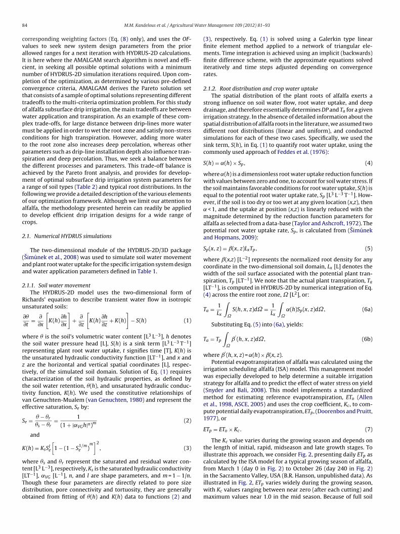
The Kc value varies during the growing season and depends onthe length of initial, rapid, midseason and late growth stages. Toillustrate this approach, we consider Fig. 2, presenting daily ETp ascalculated by the ISA model for a typical growing season of alfalfa,from March 1 (day 0 in Fig. 2) to October 26 (day 240 in Fig. 2)

in the Sacramento Valley, USA (B.R. Hanson, unpublished data). Asillustrated in Fig. 2, ETp varies widely during the growing season,with Kc values ranging between near zero (after each cutting) andmaximum values near 1.0 in the mid season. Because of full soil

M.M. Kandelous et al. / Agricultural Water Management 109 (2012) 81– 93 85

Table 2Soil hydraulic function parameters for soils of scenarios T1 (clay loam), T2, (loam) and T3 (sandy loam), as taken from Carsel and Parrish (1988).

�r (cm3 cm−3) �s (cm3 cm−3) ˛VG (cm−1) n Ks (cm day−1) l

cg(mctaDow

2

hsWzdfaadcatttmTwdogw

betaea

Fa

and model parameter/variable values, as defined in Eqs. (8) and(9). In some way, one can view our study as a sensitivity analy-sis, evaluating the impact of variable irrigation system design and

Clay loam 0.095 0.41

Loam 0.078 0.43

Sandy loam 0.065 0.41

overage by the alfalfa, soil evaporation can be considered negli-ible throughout the simulated growing season, so that Tp in Eqs.5) and (6) is equal to ETp. Typically, the alfalfa is cut about once a

onth, starting in late April, through late October, for a total of 6uttings. In HYDRUS-2D, this time series of ETp defines the poten-ial root water uptake rate, Sp. We assumed a growing season with

total of six growing cycles, corresponding with the six cuttings.espite the expected variations in alfalfa yield for the wide rangef irrigation system parameters analyzed, the alfalfa cutting datesere held fixed to these same dates (Fig. 2) for all simulations.

.1.3. Domain properties and boundary conditionsIn all HYDRUS-2D simulations we assumed that the soil is

omogeneous and that a drip-line behaves as an infinite lineource with a constant water discharge rate along the drip line.

ater flow in a homogenous soil is symmetrical in the hori-ontal direction between drip lines, so that only one-half of theomain space between drip-lines needs to be simulated. There-ore, the two-dimensional transport domain (Fig. 3) is rectangular,nd L/2 cm wide (a half-length between drip-lines). We simulated

soil domain with a depth of 200 cm, and placed the subsurfacerip line at depth D (right side of the domain). In each numeri-al simulation we assumed that the maximum rooting depth oflfalfa was similar to 200 cm, the bottom boundary of our hypo-hetical soils (Table 2). The spatial domain was discretized usingriangular finite elements (FE). Depending on drip-line distance, L,he number of elements varied between 1954 and 4897, with ele-

ent size gradually increasing with distance from the drip-line.he smallest FE size of 0.1 cm was selected around the drip-line,hereas the large FE’s were about 5 cm, furthest away from therip line. A high nodal density is required in the immediate vicinityf the drip-lines to be able to accurately model the large spatialradients in soil water pressure head caused by the infiltratingater.

A time-variable flux boundary condition was used along theoundary elements representing the emitter, so that the total dripmitter discharge when integrated around the emitter was equal

o the defined emitter discharge, q (volume per unit emitter areand time) (Gärdenäs et al., 2005). A free drainage (unit gradi-nt) boundary condition was applied along the bottom boundary,llowing for downward drainage and leaching. All other remaining

ig. 2. Assumed alfalfa ETp using ISA model during simulated growing season. Therrows indicate the different cutting times.

0.019 1.31 6.24 0.50.036 1.56 24.96 0.50.075 1.89 106.1 0.5

boundaries were assigned a zero water flux condition. Irrigationsystem design parameters were optimized using HYDRUS-2D sim-ulations for a sandy loam, loam and clay loam soil type, with vanGenuchten–Mualem soil hydraulic parameters of Eqs. (2) and (3)listed in Table 2.

2.2. Parameter optimization

Optimal irrigation system design and water application mustmaximize root water uptake and Ta, while minimizing total irriga-tion system installation costs, applied irrigation water and drainagewater losses. For that purpose we optimized drip line depth (D) anddistance (L), irrigation frequency (f), and irrigation duration (ID),with the latter two parameters enabling minimization of appliedirrigation water (AW) using a fixed emitter discharge rate. TheHYDRUS-2D model computes Ta, DP losses, and the near surface soilwater content at the alfalfa cutting times for each of the selectedparameter sets for each of the AMALGAM iterations, until it con-verges. In the final step, the search algorithm derives the Paretosolution set, consisting of a number of optimal solutions that eachrepresents a different trade-off between various optimal irrigationsystem design parameters. The trade-offs are the result of min-imizing three objective functions in Eqs. (8) or (9), and allows forselecting the optimal combination of parameters depending on rel-evance or cost differences between them. Hence, there is no singleoptimum parameter set, but the Pareto analysis provides for manycombinations of parameter values that in combination result insimilar residual values for the three combined objective functions.

Typically, parameter optimization methods such as AMALGAMare used to determine optimal parameter values by minimizingresiduals between measured and model-simulated variables. How-ever, in the present study, the objective functions are defined byminimizing residuals consisting of differences between optimum

Fig. 3. Schematic overview of the two-dimensional numerical grid used byHYDRUS-2D for the presented simulations.

8 l Wate

wt

2

pTdtddfwatSaaoiuediuIos

noliifbcaiortiHialp

fiaideplWqito

2

ft

6 M.M. Kandelous et al. / Agricultura

ater application parameters on water use efficiency, defined byhe ratio of AW to Ta.

.2.1. Irrigation system parametersThe optimized irrigation system design and water application

arameters with their upper and lower bound values are listed inable 1. These parameters define the width of the prior uniformistribution functions from which selected parameter values areaken in the AMALGAM optimization procedure. They include therip-line installation depth, D (L), drip-line distance, L (L), irrigationuration, ID (T), and irrigation frequency, f (T−1). As each of theseour parameters are expected to largely affect soil water flow, rootater uptake, and drainage, we assumed physically realistic ranges,

nd used AMALGAM to find Pareto optimal solutions that simul-aneously minimize the three different objectives considered inection 2.2.2. In essence, we seek optimum combinations of D, L, IDnd f, that maximize irrigation efficiency (as defined by minimizingpplied water (AW) and deep percolation (DP) losses) and Ta. With-ut a preference to any of the individual objective functions (OF’s)n the applied multi-criteria optimization analysis, the minimumncertainty that can be achieved for the optimized parameters isssentially determined by the trade-off in minimizing the threeifferent objectives. Specifically, if two objectives are conflicting,

t is not possible to find a single combination of parameter val-es that optimizes both of these two objectives simultaneously.

nstead, a trade-off will be determined in the fitting of both multiplebjectives, resulting in parameter variations. The Pareto solutionet defines the trade-offs with minimum OF values.

With regard to finding the optimum drip line depth (D), theear-surface soil must become sufficiently dry for each cuttingperation, without reducing crop yield. On the other hand, a tooarge installation depth may cause deep percolation losses andncrease installation costs. Whereas increasing drip-line distances cost-effective, a too large spacing may require higher irrigationrequency to maintain optimum root zone soil moisture conditionsetween the drip lines, and increase drainage losses by deep per-olation as a result. Similarly, large irrigation duration values willffect deep drainage and may cause plant water stress by introduc-ng anaerobic soil conditions, thereby reducing Ta and yield. On thether hand, applying irrigation water at values less than Tp mayeduce plant transpiration and yield even more. Therefore, irriga-ion frequency and/or water application duration must be highern summer months compared to the early and late growing season.owever, rather by varying irrigation frequency during the grow-

ng season, we chose to vary irrigation water application time, usingverage Tp rates for each of the six cutting cycles. In all our calcu-ations reported herein, we assume a constant drip-line dischargeer unit length, Q = 2.3 × 10−3 m3 m−1 h−1 (Alam et al., 2002).

Initial AMALGAM optimizations demonstrated the need for thenite element (FE) size of HYDRUS-2D domain to be flexible, toccommodate different irrigation designs and to minimize numer-cal model errors. For example, each combination of drip-lineistance (L) and drip-line installation depth (D) required a differ-nt two-dimensional nodal discretization in HYDRUS-2D. For thaturpose, we defined discrete drip installation depth (D) and drip

ine distance (L) increments of 5 and 10 cm, respectively (Table 1).e followed a similar approach for irrigation duration (ID) and fre-

uency (f) parameters, and used 1-hour and 1-day time incrementsnterval, respectively. While this approach significantly increasedhe efficiency of the multi-criteria analysis, it did not affect the finalutcome.

.2.2. Objective functionsFor general application, we define the following three objective

unctions to be minimized, OFi (i = 1, 2, 3), which in combina-ion optimize irrigation system cost and benefit by minimizing

r Management 109 (2012) 81– 93

drip-line depth (D), applied irrigation water (AW), and deep per-colation (DP), while maximizing root water uptake and croptranspiration (Ta) and distance between irrigation drip-lines (L):

OF1 = 1ωL + ωD

×[

ωD(D − Dmin)

(Dmax − Dmin)+ ωL

(1 − (L − Lmin)

(Lmax − Lmin)

)]

OF2 = 1ωAW + ωDP

×[

ωAWAW − AWmin

AWmax − AWmin+ ωDP

DP − DPmin

DPmax − DPmin

]OF3 = 1 − Ta

Tp

, (8)

The weighting factors ωD, ωL, ωAW, and ωDP allow to differen-tiate between cost of the decision variables within each objectivefunction. In particular, ωD denotes the cost of installation per unitdepth, ωL signifies the cost of unit length of drip-line, ωAW is thecost of unit volume of water, and ωDP represents either the cost ofunit volume of water or the cost needed for disposing the unit vol-ume of drained water. Realizing that minimum values of both DPand AW are zero and that DPmax = AWmax, each of the three objec-tive functions are scaled functions with values ranging betweenzero and one.

The first objective function to be minimized, OF1, minimizes theinstallation cost and equipment (i.e., drip-line) expense by mini-mizing the drip-line depth (D), while simultaneously maximizingthe distance between drip-lines (L). This performance measure issolely dependent on the actual values of L and D and does notrequire a HYDRUS-2D run to calculate soil moisture dynamics. Thesecond objective function, OF2, minimizes the cost of water byminimizing the applied irrigation water (AW) and drainage waterlosses by deep percolation (DP). The third objective function, OF3,maximizes the yield profit by minimizing soil water stress to maxi-mize plant transpiration. These latter two criteria can be computedonly using HYDRUS-2D. Differential weighting allows flexibilityin applying the objective functions to different costing scenar-ios, if applicable. For example, in OF1 one can assign the cost ofinstallation and equipment for the known specified region or evenselect either D or L as the main decision parameter by assigning azero weight to the specific parameter, if appropriate. We note thatassigning a zero weight to a parameter excludes it as an objectivefunction parameter, however, it will remain a variable parame-ter with an identified range (Table 1), thereby contributing to thePareto distribution of optimized parameters.

For most of the analysis in this study, we simplified the threeobjective functions of Eq. (8) by eliminating the cost factor, andinstead defined the combined objectives such as to optimize irri-gation system parameters by minimizing applied irrigation water(AW), while maximizing root water uptake and crop transpiration(Ta) and distance between irrigation drip-lines (L):

OF1 = 1 − (L − Lmin)(Lmax − Lmin)

OF2 = AW − AWmin

AWmax − AWmin

OF3 = 1 − Ta

Tp

, (9)

where AW = q × ID × N with N representing the number of irriga-tions of duration ID and drip-line discharge q (L T−1). Conveniently,each of the three objective functions are scaled functions with val-ues ranging between zero and one. The first objective function to beminimized, OF1, now maximizes the distance between drip-lines(L). The second objective function, OF2, minimizes applied irriga-tion water (AW) and the third objective function, OF3, seeks tomaximize plant transpiration by minimizing soil water stress. The

first two performance measures can be calculated directly from theparameters considered herein and hence do not require HYDRUS-2D simulations. Only for the third criteria, simulated soil moisturedynamics are required.

l Wate

pcwatowwoptltcfiba

2

usop(tRaebareeAfuecobisfie

2

pceds

mctfmomo(

M.M. Kandelous et al. / Agricultura

Minimization of objective functions in (Eq. (9)) might lead tohysically unrealistic results. We therefore introduce two mainonstraints. First, only those solutions were accepted for which Ta

as equal or higher than 85% of Tp. Available data indicated thatlfalfa yields were only slightly affected for such a reduction, buthat significant yield losses may occur for lower Ta values. Becausef uncertainties in crop water production function (Grismer, 2001),hich is depended on irrigation management and climatic region,e set the minimum acceptable value for Ta at 85% of Tp. Sec-

nd, cutting of the alfalfa crop requires that the average soil waterressure potential in the top 30 cm is lower (more negative) thanhe prescribed threshold value of −500 cm, (B.R. Hanson, unpub-ished data) to allow cutting and baling machinery to drive onhe field without destroying soil structure and crop. If one of theonstraints was violated we penalized the corresponding objectiveunctions so that these solutions were not further considered dur-ng the Pareto search. In general, values for both constraints cane changed for specific crops and irrigation water managementpplications.

.2.3. AMALGAM methodIn the presence of multiple conflicting objectives, it is highly

nlikely that a single optimal parameter combination exists thatatisfies all objectives. Instead, it is expected that a multi-criteriaptimization will result in considerable trade-offs, as with multi-le optimal parameter combinations, as defined by Pareto frontsin case of two objectives) or Pareto surfaces (three or more objec-ives). The AMALGAM evolutionary search method of Vrugt andobinson (2007) was used to explore the multiple parameter spacend to provide the Pareto solutions using a very computational-fficient algorithm. A detailed explanation of this approach cane found in Vrugt and Robinson (2007) and Vrugt et al. (2009),nd is beyond the scope of the current work. In brief, AMALGAMuns multiple different optimization methods simultaneously thatach learns from each other using a common population of param-ter values. The combination of optimization methods included inMALGAM are Genetic Algorithm, Particle Swarm Optimizer, Dif-

erential Evolution, and Random Walk Metropolis with adaptivepdating of the parameter covariance matrix. Improved param-ter sets are generated in an iterative way, with each algorithmontributing in proportion to its convergence rate towards a finalptimal parameter set. This approach has proven to be a credi-le and computationally efficient optimization model, especially

f many parameters are optimized simultaneously. It has shown toignificantly improve the efficiency of Pareto optimization, and isnding increasing use in many different study fields (e.g., Huismant al., 2010).

.3. Example scenarios

To illustrate the generality of the irrigation design approach, weresent three different sensitivity analyses with identical climaticonditions and design constraints (Section 2.2.2.) to evaluate theffect of (1) selected irrigation parameters (I1, I2, and I3), (2) rootistribution (R1 and R2), and (3) soil texture (T1, T2, and T3) onystem design and management (Table 3).

The effect of irrigation system parameter type on the opti-ization results was investigated using three different scenarios

onsidering simulations for the loam soil with uniform root dis-ribution. For scenario I1, we evaluated the optimization resultsor the case that minimizes drip-line depth (D), AW and DP, while

aximizing drip-line distance (L) and plant transpiration (Ta). In

ther words, scenario I1 minimizes the cost of installation, equip-ent, and water, while maximizing profit. We note that the main

bjective functions used in this study are those presented in Eq.8), but here we show the generality of the presented method by

r Management 109 (2012) 81– 93 87

assigning the arbitrary cost of unity for all decision parameters. Sce-nario I2 is the same as I1, except that we excluded the parameter Dfrom the analysis (ωD = 0), as drip installation costs for the foundedrange in this study are almost independent of installation depth(Toro, Inc., personal communication). Scenario I3 is the same as I2,except we excluded DP as an optimization parameter (ωDP = 0), inaddition, thus optimizing solely on maximum drip-line distance, L(OF1) (minimizing installation costs), and minimizing plant waterstress (OF3) (maximizing plant transpiration, Ta, and crop yield),while applying a minimum amount of applied irrigation water, AW(OF2).

It has been shown before that depth distribution of roots andassociated root water uptake has a major influence of the soil waterregime in micro irrigation (Gärdenäs et al., 2005; Hanson et al.,2008). However, since information on alfalfa root distribution insubsurface drip irrigation is absent, for the purpose of this opti-mization study we assumed two likely distribution functions thatdescribe a (1) uniform and constant root distribution across the rootzone (R1), and (2) linear decreasing rooting pattern with soil depth(R2). For the linear model, the maximum root density is at the soilsurface and decreases linearly to a zero value at the bottom of theroot zone. To minimize the number of optimizations for the rootdistribution analysis, we limited the optimizations to those for aloam soil only, setting ωD in Eq. (8) equal to zero. Moreover, we setωDP in Eq. (8) to zero, to focus the analysis on minimizing appliedwater (AW) and maximizing drip-line separation distance (L) andplant transpiration (Ta).

The soil textural and hydraulic properties affect irrigationdesign and management due to their effect on horizontal, down-ward and upward vertical water movement. Therefore, three soiltextures—clay loam (T1), loam (T2), and sandy loam (T3)–wereconsidered in this study, evaluating the effect of soil hydraulicproperties (Table 2) on irrigation design and management, for soildomains with a uniform root distribution only.

3. Results and discussion

To better understand the results of a multi-criteria parame-ter optimization with AMALGAM, we present the Pareto contourplot of Eq. (9) for a loam soil and uniform root distribution inFig. 4a, with corresponding two-dimensional bi-criterion plots forthe three-objective optimization in Figs. 4b–d. As described in Sec-tion 2.2.2, the multi-objective optimization approach used hereinmaximizes drip-line distance (L, OF1) and crop transpiration (Ta,OF3), minimizing applied irrigation water (AW, OF2). In this specificapplication, the drip line installation depth, D, was excluded fromOF1, but their values are represented among the Pareto data points.Both the contour plot and 2-dimensional Pareto graphs presentvalues for optimum parameters, with both AW and Ta normalizedwith respect to Tp. This final optimum parameter space is relativelysmall, because only limited water stress is allowed (Ta/Tp > 0.85),while simultaneously requiring dry soil conditions at all six cuttingtimes, as achieved by penalizing the objective functions if eitherconstraint is not satisfied.

We clarify that all data points of Fig. 4b–d combined, makeupthe Pareto contour plot of Fig. 4a, with each data point represent-ing a different Pareto optimal solution for any of the four designparameters combinations used in HYDRUS for which the two designconstraints were satisfied. Specifically, the contour plot of Fig. 4aprojects the Pareto surface (representing the optimal solutions forthe three OF’s) on the two-dimensional surface, with the isolines of

drip-line distance (L) representing the optimal solutions for eachspecific L. Hence, Fig. 4a and b presents identical data, with the iso-line of L = 40 cm (smallest drip-line spacing) of Fig. 4a correspondingwith the Pareto front of Fig. 4b. The solid lines of Fig. 4b–d define

88 M.M. Kandelous et al. / Agricultural Water Management 109 (2012) 81– 93

Table 3Example scenarios of sensitivity analysis.

Analysis Root distribution Soil texture Parameter included in the objective functions

Type Scenario OF1 OF2 OF3

Irrigation systemI1 Uniform Loam L, D AW, DP Ta

I2 Uniform Loam L AW, DP Ta

I3 Uniform Loam L AW Ta

Root distributionR1 Uniform Loam L AW Ta

R2 Linear Loam L AW Ta

tr

TllwAstAwsbrdar

Anbwbov

Fd(

Soil textureT1 Uniform

T2 Uniform

T3 Uniform

he so-called Pareto fronts that represent the trade-offs betweenespective objective functions.

In Fig. 4a the Pareto contour plot shows the trade-off betweena and AW, with the contour lines representing isolines of drip-ine distance, L. For example, Fig. 4a shows that for a given L value,arger Ta values will require supplying more AW to minimize soil

ater stress. Moreover, to maintain identical Ta values, values ofW must increase as L is larger. Specifically, the trade-off in Fig. 4bhows that increasing the AW/Tp ratio from 95% to 110% increaseshe value of Ta/Tp from 85% to 94%. However, a further increase ofW is much less sensitive to Ta, as optimum soil moisture conditionsill remain. The results of Fig. 4b are consistent with Fig. 4c, pre-

enting the tradeoffs between root water uptake, as representedy Ta/Tp and drip-line distance, indicating that Ta is increasinglyeduced as drip-line distance is increased. By changing drip-lineistance from 40 to 140 cm, the Ta value reduces very little, butn additional increase of drip-line distance to 240 cm reduces theelative Ta by about 10%.

When considering Fig. 4d, comparing tradeoffs between L andW/Tp, we note that increased irrigation water applications areeeded with increasing distance between drip-lines. This is toe expected as more irrigation water is required to refill soil

ater storage between irrigation events with increasing distance

etween irrigation drip-lines. The Pareto front signifies the trade-ff between L and AW. For example, large values for L result in lowalues for OF1 and high values of OF2 (Eq. (9)), as more AW must be

ig. 4. (a) Pareto contour plot of objective functions in Eq. (9), showing the trade-off betwrip-line distance. The other three graphs are corresponding two-dimensional bi-criterioTa/Tp) and drip-line distance (L), and (d) drip-line distance (L) and (AW/Tp).

Sandy loam L AW Ta

Loam L AW Ta

Clay loam L AW Ta

supplied to minimize soil water stress and to maximize Ta. In con-trast, by the same reasoning, low L-values result in larger values forOF1 and low values of OF2. Consequently, the two extreme choicesof L produce about identical values for the total OF value, therebydefining the Pareto front.

3.1. Example scenarios

As before, the Pareto points that exceeded the wetness and tran-spiration constraints were excluded from further analysis. Thus,for each different scenario the trade-off of applied water (AW) anddrip-line distance (L) are presented, whereby each point of the pre-sented bi-criterion plots corresponds to different Pareto solutions.To better illustrate the effect of drip-line depth (D), we used dif-ferent symbols for the various drip-line installation depth classesfor all bi-criterion plots of Fig. 5 (I-scenarios), 6 (R scenarios), and9 (T scenarios). We also presented the Pareto contour plot of eachscenario showing the trade-offs between drip-line installation dis-tance, L (OF1), and applied irrigation water, AW (OF2) with thecontour lines representing isolines of alfalfa transpiration, Ta (OF3).

3.1.1. Irrigation systems – I1–I3

A comparison of scenarios I1 with I2 and I3 is presented in Fig. 5,

for the case of a uniform alfalfa root distribution in a loamy soil.The plots 5a–c summarize the effect of different drip-line instal-lation depths, D, on the Pareto distributions for AW and drip-line

een relative transpiration and AW, with the contour lines representing isolines ofn plots for (b) relative transpiration (Ta/Tp) and (AW/Tp), (c) relative transpiration

M.M. Kandelous et al. / Agricultural Water Management 109 (2012) 81– 93 89

F izing Ap nd (c

i esent

dfatwTl6Totp6

eoseiad

Ftsocato

ff

ig. 5. Bi-criterion (top) and Pareto contour (bottom) plots for I-scenarios, optimarameters, (b and e) I2, excluding D and including DP as optimization parameters, a

n plots a–c are indicated with different symbols. The contour lines in plots d–f repr

istance, L. We note that for the I2 scenario, ωD is set to zero, andor I3 both ωD and ωDP values in Eq. (8) are set to zero. Similarly,s in Fig. 4, each symbol represents a high-ranked optimum solu-ion from the Pareto set of optimal solutions. Across all 3 scenarios,e find that AW must increase as drip-line distance (L) increases.

he optimization also showed that the shallowest possible instal-ation depth in this study to satisfy the soil wetness constraint was0 cm for the case of a uniform root distribution and a loamy soil.hat is, even for the I1 scenario (with drip-line depth, D, among theptimized design parameters), no optimal installation depth solu-ion was found for values of D close to the soil surface, hence, weresented only results for drip-line installation depths larger than0 cm.

A comparison of Fig. 5a–c indicates that the Pareto solutionsxhibit a tendency towards deeper drip-line installation depths asne compares I1 with I2 and I3, with the number of AMALGAMolutions for the shallow drip-line depth (D = 60 cm) decreasing. Asxpected, the minimum number of optimal solutions for D = 70 cms the largest for the I3 scenario, as deep percolation was excludeds a decision parameter for this scenario, thereby allowing for largerrip installation depths.

The corresponding Pareto contour plots are presented inig. 5d–f; with the contour lines representing isolines of relativeranspiration, Ta/Tp. When comparing Fig. 5a–c with their corre-ponding contour plots of Fig. 5d–f, we note that the Pareto frontf each scenario is represented by the isoline of Ta/Tp = 0.85 in theorresponding Pareto contour plot, as this ratio was the minimumllowable transpiration ratio. All Pareto contour plots show clearlyhat higher transpiration rates are achieved by either increasing AW

r decreasing L, or both.

Overall though, when comparing Fig. 5a–f, relative small dif-erences between the three different scenarios for D and Ta wereound. This indicates that the selected design parameters L and

W and drip-line distance, L, for (a and d) I1, including D and DP as optimizationand f) I3, excluding both D and DP as optimization parameters. The drip-line depths

isolines of relative transpiration (Ta/Tp).

AW are sufficient when optimizing SDI for alfalfa for optimumTa, but with the assumption that DP losses are relatively unim-portant. Indeed, the selected soil is a homogenous non-layeredloam, for which DP is relatively small and the installation costis not significantly affected by varying the installation depth. Forcoarse-textured or layered soils with dense layers at deeper depths,we expect the results to be different for the I2 and I3 scenarios.For these types of soils it is rather difficult to maintain favorablesoil moisture conditions required to maximize alfalfa yield andsimultaneously minimize deep water percolation. Therefore, DPis likely to vary considerably between parameter combinations,and for other than fine textured soils, this variable will becomemuch more important relative to rooting and drip-line installa-tion depths. Alternatively, it is possible to assign an appropriatecost value for deep percolated water and installation depth in Eq.(8), thereby signifying their importance in managing drip irrigationsystems.

3.1.2. Root distribution – R1 and R2The depth distribution of alfalfa roots, in relation to drip-line

depth and drip-line distance will largely affect the soil water dis-tribution in the root zone, as it will determine spatial distributionof root water uptake, soil water stress, and DP out of the root zone,and thus affecting irrigation system design and management. Wetherefore analyze the effect of two root distribution types (R1, uni-form; and R2, linearly decreasing) on irrigation system design andmanagement parameters (Fig. 6). In addition, we address the effectof root distribution on soil water and root water uptake dynamicsfor a given irrigation system (Fig. 7).

3.1.2.1. Analysis of irrigation system parameters. The effect of thetwo root distribution models (uniform and linear) on the design andmanagement of SDI system is presented in Figs. 6a and b for (R1)

90 M.M. Kandelous et al. / Agricultural Water Management 109 (2012) 81– 93

F ng AWR ndicar

ugt(poA

Fwt

ig. 6. Bi-criterion (top) and Pareto contour (bottom) plots for R1 and R2, optimizi2, linearly decreasing root distribution. The drip-line depths in plots a and b are ielative transpiration (Ta/Tp).

niform and (R2) linearly decreasing root system. The bi-criterionraphs illustrate the properties of the Pareto front for drip-line dis-ance (L) and applied water (AW) for drip-line installation depth

D) values ranging between 50 and 70 cm. Moreover, the contourlot of alfalfa relative transpiration, Ta/Tp, representing the trade-ffs between drip-line distance, L, and irrigation applied water,W, for both R1 and R2 scenario are presented in Fig. 6c and d.

ig. 7. Spatial distribution of (a) actual root water uptake distribution (ˇ′ , [L−2]) and correith columns representing the times in the middle of each of the six different cutting cy

he 60 cm depth.

and drip-line distance, L, for (a and c) R1, uniform root distribution, and (b and d)ted with different symbols. The contour lines in plots c and d represent isolines of

These plots convincingly show that larger values of L (cheaper irri-gation system) can be compensated for by larger values of AW,thereby minimizing soil water stress. For the uniform root distribu-

tion results (Fig. 6a, R1), none of the Pareto solutions derived withAMALGAM with a drip line installation depth (D) of less than 60 cmsatisfy the soil dryness constraint at harvesting times. This alsoexplains why the optimal AW values generally increase as drip-line

sponding volumetric water content (b) for R1 scenario (uniform root distribution),cles (cutting cycle is indicated in the top-right corner). The drip-line is installed at

M.M. Kandelous et al. / Agricultural Water Management 109 (2012) 81– 93 91

Fig. 8. Spatial distribution of (a) actual root water uptake distribution (ˇ′ , [L−2]) and corresponding volumetric water content (b) for R2 scenario (linear decreasing rootd uttinga

iSad(riaws

alroawnerf(ftelrsts

3ati

istribution), with columns representing the times in the middle of each of the six ct the 60 cm depth.

nstallation depth increases, simply to minimize soil water stress.imilarly, as in Fig. 5, increasing the drip-line distance will lead ton increase in AW. This highlights a general finding of our paper, andemonstrates that by increasing the distance between the drip linesless costly irrigation system) additional applied irrigation water isequired to maintain adequate soil moisture conditions in the root-ng zone to maximize yield. This trade-off is intuitively clear, anddvocates the use of the joint AMALGAM and HYDRUS-2D frame-ork considered herein to find optimal irrigation practices and

imultaneously satisfy specific constraints imposed by the farmer.In contrast to the optimization results of R1, the scenario with

linearly decreasing rooting system (R2, Fig. 6b), allows for a shal-ower drip-line installation depth (D) of 50 cm, as the maximumoot activity at the near soil surface provides for intermittent peri-ds of soil surface dryness. Moreover, the increasing soil watervailability with the shallower installation depths minimizes soilater stress as most roots are located near the soil surface. Alter-atively, increasing the drip-line installation depth for scenario R2nhances irrigation water losses by DP. Therefore, the optimizationesults in Fig. 6b show that there are no optimal irrigation systemsor D-values larger than 60 cm. Comparing the alfalfa transpirationTa) ranges for R1 (Fig. 6c) and R2 (Fig. 6d), the results show that araction of AW is likely available for the higher density of roots inhe upper part of the soil profile by capillary rise for D < 65 cm. How-ver, this upwards-directed water supply was insufficient for theoamy soil to obtain the Ta as high as that achieved for the uniformoot distribution scenario, R1. The AMALGAM optimization resultshow that this upwards-directed water supply was not sufficiento satisfy the prior defined constraints on Ta and thus no optimalolution was found for D > 65 cm.

.1.2.2. Analysis of soil water distribution and root water uptake. Asn example, we evaluate the effect of irrigation system parame-ers for fixed values of drip-line distance (L = 170 cm) and drip-linenstallation depth (D = 60 cm). This is the most economic irrigation

cycles (cutting cycle is indicated in the top-right corner). The drip-line is installed

system design, with maximum spacing of the drip-lines, and near-est drip installation to the soil surface. The optimized irrigationscheduling for this scenario resulted in a single Pareto irrigationinterval of two days only, with irrigation duration (ID) of 10 and20 h for root systems R1 and R2, respectively. To maintain favor-able soil moisture conditions and avoid water stress conditions,scenario R2 with a linearly decreasing root distribution requiresa doubling of irrigation water amounts, AW, to maintain similar Ta

values. Figs. 7 and 8 present the corresponding spatial distributionsof root water uptake (top), as represented by ˇ′(h,x,z) of Eq. (6b) andthe sink term S computed using daily values (day−1), and volumet-ric soil water content (bottom) for R1 (Fig. 7) and R2 (Fig. 8). Thesix different panels represent snapshots at the middle of each ofthe six different cutting cycles. The spatial patterns or root wateruptake are largely determined by the spatial distribution of roots,as defined by ˇ(x,z) in Eq. (5), with reductions in uptake caused bythe soil water stress function, ˛(h), in Eq. (4).

For the uniform root distribution (Fig. 7), the roots initially takeup water uniformly from the entire soil profile. In later cuttingcycles, the uptake rate varies spatially depending on available soilwater. For the first three cutting cycles, the soil wetting patternsremain in the center of the soil profile (Fig. 7b), and is symmet-ric around the drip line (D = 60 cm), causing reduced root wateruptake at the soil surface and bottom of the soil profile, and possiblysome cumulative soil water stress. However, for the latter 3 cuttingcycles, soil water redistributes downward by gravity, increasing thewetted soil root zone towards 200 cm, causing water losses by DP.

The final optimized results for the R2 root system in Fig. 8 showthat root water uptake is concentrated in the top of the soil profile(Fig. 8a), as expected, with significant water losses by DP (Fig. 8b) forthe cutting cycles in mid season (cycles 3, 4, and 5). However, most

of the AW moves upward by capillary rise as a result of large nega-tive gradients of soil water pressure head close to the surface causedby root water uptake. Maximum root water uptake occurs near thesoil surface, since there are relatively fewer roots at and below the

92 M.M. Kandelous et al. / Agricultural Water Management 109 (2012) 81– 93

F (loami iffere(

dwc

rtcalsmHh

3

aspau6fiosfmtstsmss

ig. 9. Bi-criterion (top) and Pareto contour (bottom) plots for T1 (clay loam), T2nstallation depths of 55–70 cm. The drip-line depths in plots a–c are indicated with dTa/Tp).

rip-line. Since the near-soil surface between the two drip-linesas insufficiently wetted, root water uptake there is rather low,

ausing soil water stress.In summary, for the linear root distribution case (R2) water is

equired at shallower depths and in higher amounts as comparedo the uniform root distribution (R1), thereby leading to signifi-ant water losses by DP. In contrast, root water uptake is constantnd independent of soil depth for R1, allowing AW to be muchower to maintain adequate root water uptake with no soil watertress. We note that these results may be different if the root waterodel allows for compensated uptake, as presented in Simunek andopmans (2009). These results indicate that the root distributionas a major effect on system design and irrigation management.

.1.3. Analysis of soil texture – T1–T3The bi-criterion Pareto plots for the clay loam (T1), loam (T2),

nd sandy loam (T3) soil with uniform root distribution are pre-ented in Fig. 9a–c, respectively. Additionally, the Pareto contourlots of Ta/Tp for each soil type representing trade-off between Lnd AW are shown in Fig. 9d–f. No optimal Pareto parameter val-es were determined for drip-line installation depths of 55 and0 cm for T1 (clay loam) and 55 cm depth for T2 (loam), as thener-textured soils allow for deeper optimum D-values becausef sufficient water holding capacity and low DP losses, while thehallower installations cause too wet soil conditions near the sur-ace at harvesting. Because of its higher water holding capacity,

uch lower AW is required for the clay loam than the loam soilo achieve high transpiration rates (Fig. 9d–e). However, for theandy loam soil, all of the Pareto solutions were determined fromhe shallow drip-line installation at D = 55 cm, as it is a well-drained

oil that satisfies the soil dryness constraint, while simultaneouslyinimizing DP. Although, drip-line installation at D = 55 cm was

ufficient for AMALGAM to find Pareto solutions for the sandy loamoil, it is shown in Fig. 9f that the soil water holding capacity was

), and T3 (sandy loam), optimizing AW/Tp and drip-line distance, L, for drip-linent symbols. The contour lines in plots d–f represent isolines of relative transpiration

not enough to avoid soil water stress and thus lower transpirationobtained compared to those achieved for the loam and clay loamsoils, especially at the larger drip-line distances. As Fig. 9 shows,the finer-textured soils of T1 and T2 allow for drip-line installationdepths of 70 cm, as DP losses are relatively small, while main-taining dry soil surface conditions. When comparing the Paretocontour plot of scenarios T1–T3 it is shown that larger amountsof AW are required to maintain a specified transpiration rate as thesoil texture is coarser, as corresponding soil water holding capacitydecrease and DP losses increase.

When comparing optimal drip-line distance (L) between thevarious soil types, the results show that larger L-values are pos-sible for finer-textured soils (compare T3 with T1) for any giveninstallation depth, D. This is so because the lateral soil water move-ment in clay loam (T1) is larger as compared to the sandy loam soil(T3). However, the increasing capillary rise for the clay loam soilmaintains a wet soil near the soil surface, thereby eliminating thepossibility of shallow drip line installation depths for soil types T1and T2.

4. Conclusions

An irrigation design-management modeling tool was devel-oped to simultaneously optimize subsurface drip irrigation systemdesign and management, using the optimization model AMALGAM.With this multi-criteria optimization approach, in combinationwith HYDRUS-2D modeling to simulate unsaturated soil waterflow and root water uptake, the presented sensitivity analysisprovides for optimal irrigation system and management param-eters for a wide range of conditions, including drip-line installation

depth and distance, applied irrigation water, degree of crop waterstress, and drainage losses. The so-called optimal Pareto solutionssuggest multiple trade-offs, depending on the specific parameterof most interest. Though not explicitly presented, the proposed

l Wate

oiaw

adettAieg

baoflicr

ttcoci

A

lTu

R

A

A

A

A

A

B

M.M. Kandelous et al. / Agricultura

ptimization scheme with multiple objective functions allows fornclusion of costs for the different irrigation systems and man-gement practices, thereby allowing for an economic analysis asell.

The importance of root distribution in irrigation system designnd water management has been acknowledged for severalecades, and has been evaluated by consideration of two differ-nt depth distribution functions of root architecture. We concludedhat root distribution has a large effect on optimal applied irriga-ion water, irrigation water scheduling, and deep percolation losses.lso, we recognize the general lack of information on the effects of

rrigation type on alfalfa root distribution, necessitating dedicatedxperiments to determine the influence of subsurface drip on rootrowth and spatial distribution.

Analysis of the soil texture effects showed major differencesecause of variations in water holding capacity, capillary forcesnd drainage rates between soil types. Consequently, the numberf combinations of optimal Pareto parameter values was limitedor the coarse-textured soils because of increasing deep drainageosses, whereas optimal solutions were limited to deeper drip-linenstallation depths for the finer-textured soils because of upwardapillary gradients thereby preventing dry soil surface conditionsequired for alfalfa harvesting.

The study presents examples of the capabilities of flexible irriga-ion design-management tool for alfalfa, but can be equally appliedo other crops and climates. Moreover, the presented frameworkan be utilized to include cost estimates to the multi-criteriabjective functions, thereby allowing for an extensive economicost-benefit analysis for a range of irrigation system designs andrrigation water management practices.

cknowledgements

This project was partly possible through a graduate student fel-owship by the Hydrologic Sciences Graduate Group at UC Davis.he AMALGAM source code can be obtained from the third authorpon request.

eferences

bdul-Jabbar, A.S., Sammis, T.W., Lugg, D.G., 1982. Effect of moisture level on theroot pattern of alfalfa. Irrig. Sci. 3 (3), 197–207.

lam, M., Trooien, T.P., Dumler, T.J., Rogers, T.H., 2002. Using subsurface drip irriga-tion for alfalfa. J. Am. Water Resour. Assoc. 38 (6), 1715–1721.

lfalfa fact sheet composed by the California Foundation forAgriculture in the Classroom, 2011. Available online at(http://www.cfaitc.org/factsheets/pdf/Alfalfa.pdf). Checked on 12.01.2012.

llen, R.G., Pereira, L.S., Raes, D. and Smith, M., 1998. Crop evapotranspiration guide-lines for computing crop water requirements. FAO Irrigation and Drainage PaperNo. 56, United Nations – Food and Agricultural Organization, Rome, Italy, p. 300.

SCE EWRI, 2005. The ASCE Standardized Reference Evapotranspiration Equation.Environmental and Water Resources Institute (EWRI) of the American Societyof Civil Engineers Task Committee on Standardization of Reference Evapo-

transpiration Calculation, ASCE, Washington, DC, p. 70. Available online at(http://www.kimberly.uidaho.edu/water/asceewri/ascestzdetmain2005.pdf).Checked on 12.01.2012.

reazeale, D., Neufeld, J., Myer, G., Davison, J., 2000. Feasibility of subsurface dripirrigation for alfalfa. J. ASFMRA, 58–63.

r Management 109 (2012) 81– 93 93

Carsel, R.F., Parrish, R.S., 1988. Developing joint probability distributions of soil waterretention characteristics. Water Resour. Res. 24, 755–769.

Doorenbos, J. Pruitt, W.O., 1977. Crop water requirements. Revised 1977. FAO Irri-gation and Drainage Paper No. 24, United Nations – Food and AgriculturalOrganization, Rome, Italy, p. 144.

Feddes, R.A., Kowalik, P., Kolinska-Malinka, K., Zaradny, H., 1976. Simulation of fieldwater uptake by plants using a soil water dependent root extraction function. J.Hydrol. 31, 13–26.

Gärdenäs, A.I., Hopmans, J.W., Hanson, B.R., Simunek, J., 2005. Two-dimensionalmodeling of nitrate leaching for various fertigation scenarios under micro-irrigation. Agric. Water Manage. 74 (3), 219–242.

Godoy, A.C., Pérez, G.A., Torres, E.C.A., Hermosillo, L.J., Reyes, J.e.I., 2003. Water use,forage production and water relations in alfalfa with subsurface drip irrigation.Agrociencia 37, 107–115.

Grismer, M.E., 2001. Regional alfalfa yield, ETc , and water value in western states.ASCE 127 (3), 131–139.

Hanson, B.R., Simunek, J., Hopmans, J.W., 2006. Evaluation ofurea–ammonium–nitrate fertigation with drip irrigation using numericalmodeling. Agric. Water Manage. 86 (1–2), 102–113.

Hanson, B.R., Simunek, J., Hopmans, J.W., 2008. Leaching with subsurface dripirrigation under saline, shallow ground water conditions. Vadose ZoneJ., doi:10.2136/VZJ2007.0053, Special issue “Vadose Zone Modeling” 7(2),810–818.

Huisman, J.A., Rings, J., Vrugt, J.A., Sorg, J., Vereecken, H., 2010. Hydraulic propertiesof a model dike from coupled Bayesian and multi-criteria hydrologeophysicalinversion. J. Hydrol. 380, 62–73.

Hutmacher, R.B., Phene, C.J., Mead, R.M., Shouse, P., Clark, D., Vail, S.S., Swain, R.,Peters, M.S., Hawk, C.A., Kershaw, D., Donovan, T., Jobes, J., Fargerlund, J., 2001.Subsurface drip and furrow irrigation comparison with alfalfa in the ImperialValley. In: Proc. 2001 California Alfalfa & Forage Symposium, Modesto, CA, 11–13December, p. 2001.

Meinzer, O.E., 1927. Plants as indicator of ground water. United States GeologicalSurvey Water-Supply Paper 577.

Natural Resources Defense Council, 2001. Alfalfa-the thirstiest crop. California’santiquated water policy allows large corporate farms to grow too muchwater-hogging alfalfa. Available online at http://web.archive.org/web/20010702041017/http://www.nrdc.org/water/conservation/fcawater.asp).Checked on 12.01.2012.

Putnam, D.H., Russelle, M., Orloff, S., Kuhn, J., Fitzhugh, L., Godfrey, L., Kiess, A., Long,R., 2001. Alfalfa, Wildlife and the Environment—The importance and Benefits ofAlfalfa in the 21st Century. California Alfalfa and Forage Association, Novato, CA,24 pages.

Simunek, J., Sejna, M., van Genuchten, M.Th., 2006. The HYDRUS software package forsimulating two- and three-dimensional movement of water, heat, and multiplesolutes in variably-saturated media. Technical Manual, Version 1.0, PC Progress,Prague, Czech Republic.

Simunek, J., van Genuchten, M., Sejna, M.Th., 2008. Development and applications ofthe HYDRUS and STANMOD software packages, and related codes. Vadose ZoneJournal 7 (2), 587–600.

Simunek, J., Hopmans, J.W., 2009. Modeling compensated root water and nutrientuptake. Ecol. Model. 22 (4), 505–521.

Skaggs, T.H., van Genuchten, M.Th., Shouse, P.J., Poss, J.A., 2006. Macroscopicapproaches to root water uptake as a function of water and salinity stress. Agric.Water Manage. 86, 140–149.

Snyder, R.L., Bali, K.M., 2008. Irrigation scheduling of alfalfa using evapotranspira-tion. In: Proc. 2008 California Alfalfa & Forage Symposium and Western SeedConference, San Diego, CA, 2–4 December, p. 2008.

Taylor, S.A., Ashcroft, G.M., 1972. Physical Edaphology. Freeman and Co., San Fran-cisco, California, pp. 434–435.

van Genuchten, M.Th., 1980. A closed-form equation for predicting hydraulic con-ductivity of unsaturated soils. Soil Sci. Soc. Am. J. 44, 892–898.

Vrugt, J.A., Robinson, B.A., 2007. Improvement evolutionary optimization fromgenetically adaptive multimethod search. Proc. Natl. Acad. Sci U.S.A. 104 (3),708–711.

Vrugt, J.A., Robinson, B.A., Hyman, J.M., 2009. Self-adaptive multimethod search for

global optimization in real-parameter spaces. IEEE Trans. Evol. Comput. 13 (2),243–259.

Wöhling, T., Vrugt, J.A., Barkle, G.F., 2008. Comparison of three multi-objective opti-mization algorithms for inverse modeling of vadose zone hydraulic properties.Soil Sci. Soc. Am. J. 72 (2), 305–319.