agricultural decisions relaxing credit risk constraints
TRANSCRIPT
1
Agricultural Decisions after Relaxing Credit and Risk Constraints*
Dean Karlan, Yale University, IPA, J‐PAL and NBER
Robert Osei, University of Ghana – Legon
Isaac Osei‐Akoto, University of Ghana – Legon
Christopher Udry, Yale University, IPA, and J‐PAL
DRAFT
Abstract
The investment decisions of small‐scale farmers in developing countries are conditioned by their
financial environment. Binding credit market constraints and incomplete insurance can reduce
investment in activities with high expected profits. We conducted several experiments in northern
Ghana in which farmers were randomly assigned to receive cash grants, grants of rainfall index
insurance, or a combination of the two. We find very strong responses of investment in agriculture from
the insurance. In two subsequent years, rainfall index insurance (sometimes coupled with cash grants)
was sold to farmers at randomized prices. Demand for index insurance is strong, farmers with insurance
invest significantly more on their farms, and increased insurance is associated with riskier production
choices in agriculture. Both investment patterns and the demand for index insurance are consistent with
the presence of important basis risk associated with the index insurance, and with imperfect trust that
promised payouts will be delivered. Demand for insurance in subsequent years is strongly increasing in a
farmer’s own receipt of insurance payouts, and with the receipt of payouts by others in the farmer’s
social network.
* Contact information: [email protected], [email protected], [email protected] and [email protected]. The authors thank the International Growth Centre, the Bill and Melinda Gates Foundation via the University of Chicago Consortium on Financial Systems and Poverty, the National Science Foundation, and the ILO for funding. Any opinions contained herein are those of the authors and not the funders. The authors thank Ceren Baysan, Will Coggins, Ruth Damten, Emanuel Feld, Rob Fuller, Elana Safran, Lindsey Shaughnessy and Rachel Strohm, for incredible research support throughout this project, and Kelly Bidwell and Jessica Kiessel for their leadership on this project as IPA‐Ghana Country Directors.
2
1.Introduction Economic theory tells us that in long run equilibrium, all firms should operate with the same
marginal product of labor and capital. Yet this is not what we observe in many markets. In
manufacturing, misallocations of input intensity have been shown to be a major source of low total
factor productivity (Hsieh and Klenow, 2009).
In agriculture, the predominant source of income for most individuals in developing countries
(e.g., 60% of Ghanaians are farmers (Ghana Statistical Service, 2008)), we also observe tremendous
heterogeneity in input intensity and output per acre. Capital and risk constraints may be key
impediments to investment for smallholder farmers in Ghana. Broad comparisons across countries
suggest a pattern of underinvestment for Ghana as a whole. For instance, cereal yields in Ghana
increased from about 0.82 tons per hectare in 1961 to about 1.46 tons per hectare in 2005, as compared
to increases in South Asia from 1.02 tons per hectare to 2.48 tons per hectare over the same period
(WDI 2007). These trends mimic similar trends in investment: fertilizer use in Ghana increased from
about 0.42kg/ha to 7.42kg/ha between 1961 and 2002, whereas South Asia fertilizer use increased from
about 2.55kg/ha to about 104.17kg/ha. This is just one input but still a reflection of both the low level
and growth of input use in Ghana.
To address this gap, there have been many agriculture related interventions in Ghana over the
last half century. Many of such programs have tried to encourage the intensified use of inputs such as
hybrid seeds and fertilizers, for which there is evidence of high expected returns. Experiments on
farmers’ plots across 12 districts of northern Ghana in 2010 with inorganic fertilizer in northern Ghana
showed for an additional expenditure of $60 per acre (inclusive of the additional cost of labor), fertilizer
use generates $215 of additional output per acre (Fosu and Dittoh, 2011). Yet the median farmer in
northern Ghana uses no chemical inputs.1 In focus group interviews regarding decisions on intensified
input use, farmers commonly report “lack of money” or concerns regarding the high risk from weather
and disease as key obstacles deterring investment.
The welfare gains from solving the risk problem could be huge, for three reasons. First, if risk is
discouraging investment (e.g., see Carter and Barrett, 2006; Christiansen and Dercon 2010, JDE
forthcoming; Rosenzweig and Binswanger, 1993), and marginal return on investments are high, the
returns to removing risk could be high. Existing evidence from fertilizer in northern Ghana suggests that
these returns are indeed high.2 Second, agriculture in northern Ghana is almost exclusively rain‐fed.
Thus weather risk is significant and index insurance on rainfall has promise (and also avoids adverse
selection and moral hazard problems with crop insurance). Third, we have strong evidence that rainfall
shocks translate directly to consumption fluctuations (Kazianga and Udry, 2006). Thus mitigating the
risks from rainfall should lead to not just higher yields but also smoother consumption.
To understand how capital and risk interact, and under what circumstances lead to
underinvestment, we experimentally manipulate the financial environment in which farmers in northern
1 This fact is derived from the control group of farmers in the first year of our survey, described in section 3 below. 2 See also Fafchamps et al. (2011), Udry and Anagol (2006).
3
Ghana make investment decisions. We do so by providing farmers with cash grants, grants or access to
purchase rainfall index insurance or both. The experiments are motivated by a simple model which
starts with perfect capital and perfect insurance markets, and then shuts down each. Farm investment is
lower than in the fully efficient allocation if either market is missing (and land markets are also shut
down, given the restrictions of the land tenure system in northern Ghana). If credit constraints are
binding, then provision of cash grants increases investment, but the provision of grants of insurance
reduces investment. In contrast, when insurance markets are incomplete, provision of cash grants has a
minimal impact on investment, but investment responds positively to the receipt of an insurance grant.
To test these predictions, we turn to a three‐year multi‐stage randomized trial. In year one, we
conducted two experiments. The first is a 2x2 experiment: maize farmers either received (a) a cash grant
or no cash grant, and (b) a rainfall insurance grant or no rainfall insurance grant. In the second
experiment, to a separate group of farmers, we sold rainfall insurance at prices ranging from one eighth
of actuarially fair to market price (i.e., actuarially far plus a market premium to cover servicing costs). In
year two, we conducted another cash grant experiment, but only offered rainfall insurance for sale
(again, at randomly different prices) rather than giving some out for free as in year one. In year three,
we did not conduct another cash grant experiment, but the insurance pricing experiment continued.
Four elements distinguish our data and experiments: (1) the cash grant experiment to measure
the effect of capital constraints on investment and agricultural income (most of the existing
complementary research is on the insurance component), (2) the provision of free insurance, in order to
observe investment effects on a full population rather than just those willing to buy (a notable
complementary study is Cole, Gine and Vickrey, 2011, who provide grants of free insurance to farmers in
India), (3) multi‐year setup, and (4) a complete demand curve, from nominally positive (8% of actuarially
fair) all the way to approximate market prices (i.e., actuarially fair plus a 50% premium to cover servicing
costs). In the Discussion section of this paper we relate our results to the complementary literature on
risk and capital capitals for agriculture.
We find strong responses of agricultural investment to the rainfall insurance grant, but relatively
small effects of the cash grants. The salient constraint to farmer investment is uninsured risk: when
provided with insurance against the primary catastrophic risk they face, farmers are able to find
resources to increase expenditure on their farms. At the actuarially fair price, 40 to 50 percent of
farmers demand index insurance, and they purchase coverage for more than 60 percent of their
cultivated acreage. Patterns of insurance demand are consistent with farmers being conscious of the
important degree of basis risk associated with the index insurance product. Farmers do not seem to
have complete trust that payouts will be made when rainfall trigger events occur, so the demand for
index insurance is very sensitive to the experience of the farmer and others in his social network with
the insurance product. Demand increases after either the farmer or others in his network receive an
insurance payout, and demand is lower if a farmer was previously insured and the rainfall was good,
thus no payout was made.
In the next section, we provide a simple model of investment in a set of different financial
environments. Section 3 describes the empirical setting, the experimental interventions, and the data
4
collection process. Section 4 provides the key results on the effects of cash and insurance grants on farm
investment. Given these results, section 5 provides a model of the demand for insurance and
agricultural investment when farmers do not face binding credit constraints. Section 6 provides results
on the demand for index insurance, characterizes patterns of investment given the availability of index
insurance at randomized prices, and explores the effects of social interactions on insurance demand.
Section 7 discusses the implications of our results in the context of the literature, and Section 8
concludes.
2.InvestmentandtheFinancialEnvironment In an environment with well‐functioning markets, including markets for insurance and capital,
the standard neoclassical separation between production and consumption would hold and farmers’
input choices on a particular plot would be independent of their wealth and their preferences.
Investment in inputs would maximize the present discounted value of the (state‐contingent) profits
generated by those investments. Where insurance markets are imperfect or absent, or credit constraints
bind, separation no longer holds, and the randomized provision of capital grants or insurance that pays
off in certain states may influence farmers’ investment choices. The purpose of this section is to provide
a simple model that permits us to use the investment response to capital grants and/or the provision of
insurance to draw conclusions about the financial environment farmers face.
A minimal model sufficient for this purpose includes 2 periods, production, risk, and the
appropriate financial markets. Preferences over consumption in the first period (c) and in the various
states of the second period ( )sc are
(1) ( ) ( )s ss S
u c u cb p+ å
Start, naturally enough, with a complete markets environment in which the household (with exogenous
cash on hand Y) has access to a market on which it can buy (or sell) a risk free asset (a) which earns (or
pays) interest R 1
( ,
to simplify notation later), and also access to an informal insurance market, in
which securities ( si ) pay off in state s and are available at price sp . A farmer of type has a production
technology that provides second period output equal to ( ; )sf x in state s after inputs x are committed
in the first period. In anticipation of our two‐pronged intervention, let k denote a cash grant provided to
the farmer in the first period, and sk be a state‐contingent payout promised if s occurs in the second
period. The household maximizes (1) subject to
(2) ( ; )
0.
s ss S
s s s s
c Y x a p i k
c f x Ra i k
x
q
= - - - +
= + + +³
å
5
The household chooses si such that
(3) '( ) '( )s sp u c u c
for all s, and farm investment satisfies
(4) ( ; )
1 ss
s
f xp
x
.
With complete markets, farm investment is independent of resources (Y) and preferences, as we
expect.3 Neither a capital grant nor an insurance policy has any influence on farm investment:
(5) 0.s
dx dx
dk dk
We now introduce, in turn, capital constraints and imperfect insurance markets. To simplify
some of the notation which follows, we let { , }S L H with ( ; ) ( ; ).L Hf x f x We also assume that
the marginal product of inputs (x) is lower in L than in H; this of course need not be the case and is a
substantive assumption. It corresponds to farmer accounts of their practices and understanding in
northern Ghana.4 To simplify some of the expressions below, we’ll make the extreme assumptions that
both the marginal return on inputs and the absolute return is zero in the low state (i.e.,
( ; )( ; ) 0,L
L
f xf x
x
) but these are not essential for any of our results.
2.1CapitalConstraints
Suppose that borrowing is not possible, so to (2) we add the constraint that 0.a We will
consider situations in which this constraint binds. Obviously we cannot permit trading a full set of
actuarially fairly priced contingent securities, because that would permit unlimited borrowing.
Therefore, we shut down the insurance market entirely and set 0si . But we are interested in
examining the consequences of capital constraints when risk is not salient, so we eliminate risk by
presuming the existence of informal risk pooling such that
(6) ( ) .s s s ss
c c f x ra kp é ù= = + +ë ûå
3 If the insurance is actuarially fair, then s sRp , in which case a is redundant (it is replicated by purchasing
1
#( )S units of each contingent security).
4 There is agronomic evidence as well. See Amujoyegbe et al. (2007).
6
There is informal consumption pooling and every household consumes the expected value of its
consumption in any state.5 With 0a binding the first order conditions become
(7) ( ) ( )u c ru cb¢ ¢>
and
(8) ( ; )
( ) ( ) .HH
f xu c u c
x
qb p
¶¢ ¢=
The implicit function theorem immediately implies
(9) 0 .L
dx dx
dk dk> >
The capital grant reduces the shadow price of the binding borrowing constraint, raising the relative
value of consumption in the future and therefore inducing higher investment in x. In contrast, the
promise of future resources, even in the bad state L, increases that shadow price and lowers the relative
value of consumption in the future. Hence investment in x falls with promised contingent payments.
2.2ImperfectInsurance
In the extreme, there is no informal insurance: 0si . The household chooses x such that
(10) ( ) ( ; )
1 .( )
L L H
H H
u c f xR
u c x
p qp
é ù¢ ¶ê ú+ =ê ú¢ ¶ë û
Let 0 0{ , }a x solve (10). If u(.) is CARA, then0x solves (10) for any level of k, because
0( ; ) .H L H Lc c f x kq- = -
In contrast, increases in promised payouts in the bad state reduce the LHS of (10). Therefore, with CARA preferences, the absence of informal insurance implies
(11) 0 .L
dx dx
dk dk= <
The extreme conclusion that 0dx
dk relies on the CARA assumption. For many other preferences – e.g.,
CRRA, the risky investment in x will increase with the capital grant because the absolute degree of risk aversion will fall as wealth increases.
2.3CapitalConstraintsandImperfectInsurance
5 We have implicitly assumed that the risk pooling group is sufficiently diverse that there is no aggregate risk. This extreme assumption serves to focus on the implications of binding credit constraints in the absence of any risk‐based motivation for moving resources across periods.
7
With 0a binding, (8) remains a first order condition, and since a=0, c Y x k and
( ; ) .s s sc f x k The implicit function theorem implies
(12) 0 .s
dx dx
dk dk>
To summarize, if farmers have access to complete insurance and capital markets, investment is invariant to both capital grants and the provision of free insurance. With binding credit constraints (either with or without complete insurance markets), investment rises with a capital grant and falls when insurance is provided. When credit constraints are not binding but insurance is imperfect, investment rises with the provision of insurance, and may rise with a capital grant.
3.TheSetting,theInterventionsandDataCollection
3.1 Year One: Sample Frame and Randomization for Grant Experiment
In order to have a rich set of background data on individuals and a representative sample frame, we
used the Ghana Living Standards Survey 5 Plus (GLSS5+) survey data to form the initial sample frame.
The GLSS5+ was conducted from April to September 2008 by the Institute of Statistical, Social and
Economic Research (ISSER) at the University of Ghana – Legon in collaboration with the Ghana Statistical
Service. The GLSS5+ was a clustered random sample, with households randomly chosen based on a
census of selected enumeration areas in the 23 Millenium Development Authority (MiDA) districts6.
From the GLSS5+ sample frame, we then selected communities in northern Ghana in which maize
farming was dominant, and then within each community, selected the households with some maize
farming, but no more than 15 acres of land. Within each household, we identified the key decisionmaker
for farming decisions on the main household plot, which was typically the male head of household
(except in the case of widows). Our sample frame is over 95% male as a result. This yielded a sample
frame of 502 households. We refer to this as Sample Frame 1, or the Grant Experiment sample frame.
We then randomly assigned the 502 households to one of four cells: 117 to cash grant, 135 to
insurance grant, 95 to both cash grant and insurance grant, or 155 to control (neither cash grant nor
6 Ghana has 170 districts in total, twenty of which are located in the Northern Region. MiDA is the Ghanaian government entity created to lead the programs under the compact between the US Government Millennium Challenge Corporation (MCC) and the Ghanaian government. Although the sample frame for this study was generated from the GLSS5+, the interventions described here were independent of MiDA and MCC.
8
insurance grant).7 The unit of randomization was the household, and the randomization was conducted
privately, stratified by community. We did not have the GLSS5+ data prior to the randomization, and
thus were not able to verify orthogonality between assignment to treatment and other observables.
When cash and rainfall insurance grants were announced to farmers, they were presented not as part of
a randomized trial but rather as a service from a research partnership between IPA and the local
nongovernmental organization Presbyterian Agricultural Services (PAS).8
Table 1 shows summary statistics, mean comparisons of each treatment cell to the control, an F‐test
from individual regressions of each covariate on a set of three indicator variables for each treatment
cell, and an F‐test from a regression of assignment to each treatment cell on the full set of covariates.
3.2 Year One: Insurance Grant Design
We designed the insurance grant in collaboration with the Ghanian Ministry of Food and Agriculture
(MoFA), Savannah Agricultural Research Institute (SARI) and PAS, and secured exclusive permission from
the Ghana National Insurance Commission to research takeup and effects of a non‐commercial rainfall
index insurance product designed to make farmers feel insured. We held focus groups with farmers to
learn about their perception of key risks and about the types of rainfall outcomes likely to lead to
catastrophically low yields. Whilst rainfall data for Ghana was available from 1960 onwards from the
Ghana Meteorological Service (GMet), equivalent data was not available for crop yields, leading to our
decision to use ICRISAT yield data from Burkina Faso instead. Given the limitations of this historical
data, our decision about the trigger rainfall amounts for insurance payouts was made largely on the
basis of our qualitative discussions with our Ghanaian partners and farmers. The value of insurance
payouts in case of catastrophically low yields was set to be equal to mean yields in the GLSS5+. We also
were concerned with product complexity and farmer understanding, and acknowledge that simplicity
came at the expense of increased basis risk (see Hill and Robles (2010) for an analysis and innovative
approach using laboratory experiments to assess farmer perception of basis risk and insurance fit). The
7 Since the budget for this research included the cost of the intervention and since the size of the sample frame
was not fixed, we optimized statistical power by increasing the size of the control group relative to the treatment
groups. However, since the exact formula for optimal power depended not just on the relative cost but also on any
change in variance, we did not solve this analytically but rather approximated.
8 The script for the field officers for the insurance grant, for example, was as follows: “I am working for NGOs called Innovations for Poverty Action and Presbyterian Agriculture Services. We are trying to learn about maize farmers in the Northern Region, and in (Tamale Metropolitan / Savelugu‐Nanton / West Mamprusi) district. As part of this research, you are invited to participate in a free rainfall protection plan called TAKAYUA Rainfall Insurance, which I would like to tell you about.” Control group households were informed that others in their community had received grants but that limited resources did not allow everyone to receive one, and that the selection was random and thus fair to everyone.
9
trigger for payouts was determined based on the number of dry or wet days in a month (where either
too much or too little rainfall triggered a payout). The payout amount was chosen in order to
approximately cover 100% of a full loss, or roughly GHS 100 per acre of maize grown.
We used five rainfall gauges in 2009. The mean distance from plots to the rain gauge ranged from
9.7km to 37.6km. Appendix Table 1 provides summary statistics on distance to farmer homesteads in
our sample and rainfall for each gauge, and Figure 7 provides a map of the area and location of
communities and rain gauges in the study.
Around March of 2009, we sent insurance marketers to those villages selected to receive the
insurance offer, where a Ministry of Food and Agriculture‐appointed farmer and PAS‐employed field
officer assisted us in identifying those farmers selected to receive the insurance offer. During these
individual visits with selected farmers, marketers described the insurance policy in a clear and simple
way, left a copy of the policy document with each farmer, and informed the farmer he would have
approximately two weeks to decide whether to take up the offer. Marketers returned to each farmer
two weeks after this visit and issued a certficate to those farmers agreeing to take up the product. In this
case, where the product was offered at no cost, 100 percent of farmers took it up.
A total of 230 policies were issued to farmers free of cost in year one, covering a total of 1,159.5
acres, for an average of about five acres per farmer. We granted each farmer insurance coverage for the
number of acres they reported farming maize in the GLSS5+. One payout was made to 171 farmers in
July of 2009 at GHS 60 per acre, or roughly 60 percent of estimated loss. The average payout was GHS
243 per farmer, conditional on receiving a payout.9 Payouts were made within two weeks of the rainfall
shock that had triggered the payout, with the intention that the cashcould have been applied to
investment in labor during harvest. For this reason, the analysis will focus on investments made before
the rainfall shock, such as number of hectares of land cultivated, fertilizer used, etc.
3.3 Year One: Cash Grant Design
For those in the cash grant treatment, we first announced the grant and explained it the same way as
the insurance grant: as a collaboration between IPA and PAS to help smallholder farmers and learn more
about farming in northern Ghana. We made three key design decisions concerning the cash grant
treatment: the timing, the amount, and whether to transfer in‐kind goods or cash. For the timing, we
decided to individualize delivery of the grant based on the farmers’ stated preferences and intentions
9 In order to test an involuntary soft commitment to spend the insurance payouts on large indivisible investments, we also randomized the size of the bills in which the cash was delivered. The options were small bills (i.e., usable in their local community) or large bills (realistically not usable unless they travel to Tamale, the closest major city, and also where they typically would buy farm inputs in the following season). We do not report on the results from that sub‐experiment in this paper.
10
about use of the grant. Thus if they reported it would all go to seed, they would receive the cash at time
of planting, whereas if they reported half would go to seed and half to labor for harvest, half would be
delivered during the planting period and half at the harvest. With regard to the amount of the grant, we
decided to make it a fixed total amount per acre of land, despite the distributional consequence of this
from a policy perspective, because our interest here is in studying returns to capital. We delivered GHC
60 per acre (up to 15 acres) to 212 farmers selected to receive cash grants. We determined the amount
by working with MoFA to determine the total cost of inputs and labor costs as per the MoFA
recommended maize farming practices. Finally, we decided to give cash rather than in‐kind. This was
done in order to allow the farmers to use the resources as they thought best. Due to budget constraints,
we were unable to randomize the implementation of the grant in order to test out the various options
on amount, timing and cash vs. in‐kind delivery.
3.4 Year Two: Expanded Sample Frame for Insurance Product Pricing Experiment
For year two, we then expanded the sample frame in order to conduct an Insurance Product Pricing
Experiment. The second year insurance coverage also was redesigned and renamed to Takayua (which
means “umbrella” in the local Dagbani language), and calibrated to trigger per‐acre payouts after seven
or more consecutive “wet” days (over 1mm of rainfall) or after twelve or more consecutive “dry” days
(1mm or less rainfall). Payouts under Takayua were promised to be delivered two weeks after the dry or
wet spell had been broken.
The Insurance Product Pricing Experiment included the Grant Experiment sample frame from Year 1,
as well as two new sample frames: new households in Grant Experiment communities (Sample Frame 2),
and entirely new communities (Sample Frame 3). Randomization was at the community level in order to
facilitate communication and avoid confusion that would result from offering insurance at different
price levels within a single community.
For the expansion in communities already part of the Grant Experiment (Sample Frame 1), we first
conducted a census in order to select additional households for the sample. Using our census, we
applied the same filter as in the Grant Experiment (maize farmers with fewer than 15 acres). This yielded
644 additional households, which combined with the original 502 from the Grant Experiment yielded a
sample frame of 1,146. We then randomly assigned each community to be sold the insurance product at
a price of either GHC 1 or GHC 4, and then randomly drew 1,101 of the 1,146 to be sold the insurance,
with the remainder being in a control group of individuals not offered the insurance. Both prices
represent considerable subsidies, as the actuarially fair price was about eight cedis per acre. Offers were
made in November 2009, and we sold 407 out of 480 offered at 1 GHC, and 261 out of 393 offered at 4
GHC.
We then added a new community sample frame (Sample Frame 3) in order to test actuarially fair
and market‐based prices for the same insurance product. First we randomly selected 12 new
11
communities from maps of the areas that delineated all communities within 30 kilometers of one of the
rain gauges. We then completed a census in each community [with what data collected? A quick list
here would be good] and filtered the sample using the same criteria as the Grant Experiment (maize
farmers with fewer than 15 acres). We drew 228 households (19 per community) into the sample frame.
We then randomly assigned each community to receive insurance marketing at either the estimated
actuarially fair price (GHC 8 or 9.5, depending on the rain gauge), or the estimated price in a competitive
market (GHC 12 or 14, depending on the rain gauge). and then offered all 228 newly selected farmers
an opportunity to purchase the insurance product. Offering the insurance product at several prices,
including at the estimated actuarially fair and competitive market prices, allowed us to measure demand
for the product at different prices and to further refine a demand curve for rainfall index insurance in
the region. Offers were made in March 2010, and we sold 17 out of 38 policies offered at 8GHC, 31 out
of 76 policies offered at 9.5 GHC, 7 out of 38 policies offered at 12 GHC and 6 out of 76 policies offered
at 14 GHC.
For both sample frames, each farmer who purchased insurance was visited four times as part of the
marketing. During the first visit, a marketer educated individual respondents about the Takayua product
and its price. During the second visit, a marketer returned to sign contracts with and collect premiums
from respondents. During the third visit, a marketer issued a physical policyholder certificate, including
details on the policyholder and acreage covered, to each policyholder. During the fourth visit, an auditor
from IPA verified understanding of the terms and conditions of Takayua with roughly 10 percent of
farmers who had chosen to take up the product.
To better understand farmers’ comprehension of the policies and learn about their perceptions of
basis risk, we conducted a post‐harvest survey with 672 of 729 Takayua policyholders following the year
two harvest in December 2010. The survey revealed that 41.3 percent of farmers who received one
payout found it sufficient to cover damages sustained, but that 97.9 percent of the treatment group
indicated willingness to purchase the product again for the 2011 farming season.
3.5 Year One FollowupSurvey \ Year Two Baseline Survey
In January through March 2010, we attempted to survey 1,132 farmers, the union of the 488 households
in Sample Frame 1 (the Grant Experiment) and 644 households in Sample Frame 2 (the year two
Insurance Product Pricing Experiment farmers that were from existing communities).10 We completed
1,087 of 1,132 surveys, for an overall response rate of 96 percent.
10 The product pricing experiment in new communities took place immediately after this survey was completed, thus Sample Frame 3 is included in the 2011 followup survey but not this one. Four farmers were dropped between years due to [XX].
12
This comprehensive survey included many components: household socioeconomic indicators
(including education, health, waged labor, and formal employment), plot‐level farming questions
(including land tenure, seeds, chemical inputs, agricultural labor, harvest, crop sales and storage),
livestock, fishing, agricultural processing, household assets, expenditures, consumption, social
networks, insurance knowledge, risk perceptions and finance (including borrowing, lending, savings,
other income, and transfers).
3.6 Year Two: Cash Grant Experiment
In the year two Cash Grant Experiment conducted between May and June 2010, we repeated the cash
grant to a newly randomized subset of 363 farmers from Sample Frame 2 (i.e., thus there was no
overlap with those in the year one capital grant experiment). The cash grant was GHC 350 per
household, regardless of acreage, and the entire amount was given to the farmers at a single time
(rather than spread out over the season as we did in the first year).
3.7 Year Two: Insurance Payouts
Two of five rainfall stations triggered payouts totaling 78,400 GHC in 2010. The Tamale (Pong) station
measured eight consecutive wet days in late August triggering a payout of 20 GHC per acre to 125
individual farmers with 785 acres. The total payout was GHC 15,700. The second payout was made when
the Walewale station recorded 11 consecutive wet days in late September triggering a payout of 50 GHC
per acre to 225 individual farmers with 1,254 acres. The total payout in Walewale was GHC 62,700.
These payouts were made within two weeks of the trigger event, in fulfillment of the contract terms
established between IPA and Takayua policyholders.
[xx LS checking on the protocols/audits herexx]
3.8 Year Two: Follow‐up Survey
In February and March 2011, we conducted a second follow‐up survey targeting 1,362 households, the
union of Sample Frame 1 (the year one Grant Experiment), Sample Frame 2 and Sample Frame 3 (the
year one Insurance Product Pricing experiment). We reached 1,284 of the 1,358 households, for an
overall response rate of 94.3 percent.
The comprehensive survey was conducted using electronic netbooks. In order to ensure data
quality, the instrument was programmed to ask for confirmation of and updates on last year’s data,
through “preloading” reported data about household members, plots, employment, assets, livestock
and loans. The survey also asked for new data on areas including harvests, crop storage and sales,
chemical use, seed sources, ploughing, livestock, income, expenditures, assets, loans, agricultural
processing, education, health, household enterprise and formal employment.
13
3.9 Year Three: Commercial Product and Pricing Experiment
In May 2011, we then negotiated a partnership with the Ghana Agricultural Insurance Programme
(GAIP) to market GAIP’s commercial drought‐indexed insurance product, a product reinsured by Swiss
Re and endorsed officially by the National Insurance Commission. Due to the increased complexity of
the commercial product (compared to the original non‐commercial product from years one and two),
individual marketing scripts and protocols emphasized transparency about the product, named Sanzali,
the Dagbani word for “drought”. Sanzali was divided into three stages based on the maize plant’s
growth stage, and each stage included one or two types of drought triggers (cumulative rainfall levels
over dekads [ten day periods], or consecutive dry days). Because the Sanzali product was significantly
more conservative than the Takayua product, the marketing session this year included an in‐depth
comparison of terms and historical payouts. The Sanzali product was offered at an actuarially fair price
of GHC 6 per acre, as well as a subsidized price of GHC 3 per acre and a market price of GHC 9 per acre.
The pricing assignments were randomized by community each week to control for demand, with 23
communities (31.9 percent) in the market price cell, 23 communities (31.9 percent) in the actuarially fair
and 26 communities (36.2 percent) in the subsdized price cell.
The same farmers from the year two pricing experiment were included in this year three pricing
experiment. We made contact with 982 of 1,101 farmers (89.1 percent) and sold a total of 572
premiums (58.2%), covering a total of 3,187 acres. As with year two, each farmer was visited up to four
times. Demand was 78.1% at the subsidized GHC 3 per acre price, 67.4% at the actuarially fair GHC 6 per
acre price, and 54.5% at the market price GHC 9 per acre.
As with the second year, three to seven days after the marketing visit, IPA staff conducted audit
visits with ten percent of the insurance group to test their comprehension of the product. Audit reports
confirm that farmers had a clear understanding of the product, including complex ideas such as
cumulative rainfall per dekad. IPA also conducted informal interviews to gain insight into how
smallholders financed their insurance purchase, finding that smallholders made their purchases through
informal loans, produce sales, gifts, or small ruminant sales.
3.10 Year Three: Insurance Payout
The insurance product in year three (2011) did not trigger any payouts.11
11 Although not reported in this paper, we conducted a notification experiment after the realization that there
would be no payout. We were concerned that silence may lead to longer term mistrust. Thus in December 2011,
we conducted a notification experiment and harvest survey with the 572 Sanzali policyholders. In the notification
experiment, [xx] policyholders were notified individually and [xx] policyholders were notified as part of a group
about rainfall measurements recorded at their nearest rain gauge and about insurance outcomes. The notification
experiment served two purposes: (1) to respond to requests made by policyholders during the 2010 harvest survey
14
4.CapitalGrants,InsuranceandInvestment Figures 1‐4 summarize the consequences for farm investment of the randomized provision of
either capital grants, rainfall index insurance, or both. The first panel of Figure 1 shows that the CDF of
total expenditures on the farms of households who received free insurance is strongly shifted to the
right of that of control group farmers. The strongest effects are in the left tail of the distribution of farm
expenditures: the 25th percentile increases by about US$300, from a base of a little more than US$375.12
In contrast, the second panel shows that there is no strong difference between the control group and
the capital grant group: the 25th percentile of the grant group is about US$100 higher than that of the
control group, but the difference is eliminated from the median onward. The final panel shows that the
CDF of total expenditures for the group that received both the capital grant and insurance is also shifted
to the right of that of the control group; but there is little substantive difference between the CDFs of
the group that received only insurance (panel 1) and the group that received both insurance and capital
(panel 3).
The effects of capital grants and insurance on total expenditure are not those that one would
expect to see for farmers facing binding credit constraints. Farmers in the insurance group were
promised future resources in certain states of the world, and given nothing up front. With binding credit
constraints, this would have induced farmers to reduce investment on farming activities; instead, we see
a dramatic increase.
Figure 2 Panel 1 documents a similar increase by the insurance group in expenditures on farm
chemicals, largely fertilizer. Figure 2 Panel 2 shows that the capital grant group also strongly increased
their expenditure on chemicals, as did the group that received both capital grants and insurance.
In Figure 3, we see that insurance also has a positive effect on the acres cultivated by farmers
(the step pattern is driven by clustering at unit values of reported cultivated acres), but that there is no
difference between the CDFs of area cultivated by the control and capital grant groups. Harvests may be
higher for the group that received insurance than for the control group (Figure 4), but the difference is
relatively small. However, the group that received both insurance and capital does have a CDF of harvest
values that is distinctly shifted to the right of that of the control group. We will discuss this pattern
further below, where we argue that it and other evidence may reflect the salience of both basis risk and
the impact of the capital grants on the expectations of policyholders that insurance payouts will be
made when trigger events occur.
and 2011 insurance marketing to provide information about insurance outcomes at the end of each coverage
period, and therefore to build upon established trust between marketers and communities, and (2) to test group
education rather than individual education to ensure the same treatment effect could be generated at lower cost,
and therefore to inform planning for community‐level marketing activities in 2012.
12 We use an exchange rate of 1.33 Ghana Cedi to US$1 for this paper, although over the two years of the study the exchange rate fluctuated between [] and [].
15
The index insurance product we designed had the feature that payouts would be made quickly –
within a week – of the realization of a trigger. Thus some payouts happened mid‐season, not post‐
harvest. This leads to the natural question as to whether the observed investment responses could
simply reflect the insurance payouts, and not a behavioral response upon receiving the insurance
contract? Figure 3 is key to examine this issue, because cultivated area is determined during the plot
preparation stage of the farming season, before any insurance payouts could be made. Thus although
we cannot rule out any later investments happening with the insurance proceeds from negative shocks,
we do clearly observe some behavioral response prior to any cash infusion.
In Table 2 we show further evidence that the realization of payouts is not the source of the
investment effect of insurance. “Prospective Payout” is the amount that a farmer would have received
had he had the rainfall insurance; of course, only the “insurance” and “both” group farmers actually
received this payout. The total costs of cultivation, expenditures on chemicals, and cultivated area is
higher for the insurance and both treatment groups than for the control group (although the difference
is not always statistically significant), but there is no evidence that the actual payouts of insurance
contribute to this increase.
5.ModelingtheDemandforInsuranceandInvestment
We focus on an environment in which farmers are not confronted with binding credit
constraints, but in which they do not have access to robust informal insurance mechanisms. We
continue to consider a world with two states and examine the demand for rainfall index insurance at
price p that pays off in state L. The household’s budget constraints are now
(13) c Y a x pI
(14) ( ; )H Hc f x Ra
(15) ( ; )L Lc f x Ra I
The first order conditions for I, a, and x are
(16) '( )
'( )L
L
u c
u c p
(17) '( ) '( ) '( )H H L Lu c u c u c
(18) ( ; )
'( ) '( ) HH H
f xu c u c
x
16
If LpR
then the insurance is actuarially fair, and we have the familiar results that L Hc c c . In
such a case, consumers demand full insurance and investment in the risky agricultural activity is optimal.
Index insurance, however, unless subsidized, is rarely actuarially fair but rather sells at a premium to
cover the transaction and operations costs for the company if a competitive market, and also economic
profits if non‐competitive. When ,LpR
i.e., above actuarially fair, households demand less than full
insurance and .L Hc c c Therefore,
( ; )H
H
f xR
x
.
Farm investment is lower than it would be in the case of actuarially fair insurance, because the
investment pays off more in the state in which resources are less valuable.
The presence of an insurance market, even at prices above actuarially fair, is associated with a
separation result. Combining (16)‐(18) we have
(19) ( ; )
.1
HR f x
Rp x
Despite the fact that there is not full insurance and households are risk averse, production decisions are
separable from preferences and from the riskiness of the farmer’s land.
We suppose that increasing corresponds to a mean preserving spread of f:
( ; ) ( ; ) ( ; ) ( ; )r r s sH H L L H H L Lf x f x f x f x for all ( , )r s , and
( ; ) ( ; ) for all .r s r sH Hf x f x In order to focus on the effect of the risk properties of the plot
on insurance demand and investment, rather than on the direct production interactions between and
x, we make the counterfactual assumption that( ; ) ( ; )
.r s
H Hf x f x
x x
With this assumption, (19)
implies that .s rx x This is a consequence of the insurance market itself; it holds regardless of the
preferences of the two farmers. There is inefficiently low investment when insurance is priced at higher
than the actuarially fair rate, but there is no variation across farmers.
Insurance demand varies with the riskiness of the plot. Suppose farmers s and r have identical
CARA preferences again. (16) and (17) imply
(20) 0s r s r s rL L H Hc c c c c c
If Y is the same for s and r, then 0 when the insurance price is actuarially fair, and grows
monotonically as the price of insurance increases: it represents the additional cost of insurance to the
farmer with riskier land. Therefore,
17
(21) ( ( ); ) ( ( ); ) ( ( ); ) ( ( ); )r s r s r sH H L Lf x p f x p f x p f x p I I
and the farmer with riskier plots demands more insurance at every price. However, there is no
additional ‘selection’ into higher (or lower) risk farmers as the price rises.
This conclusion depends on two assumptions that are unlikely to be correct. First, it depends on
the CARA assumption. With other preferences, for example CRRA, increases in p can be associated with
relative selection of riskier plots into the insured pool. Second, it depends on the lack of a direct
technological relationship between the riskiness of the plot and the marginal product of investment. We
cannot speculate on the sign or magnitude of any such technological relationship; this is an empirical
question that to our knowledge has never been examined.
5.1BasisRisk
An essential aspect of any actual index insurance product is basis risk. Insurance payouts are not
identical with the realization of bad states. We introduce basis risk by adding a state N in which there is
no payout. We suppose that ( ; ) ( ; )N Lf x f x ; this is not necessary for the analysis but is convenient
for reasons that will become apparent in the next subsection. Consumption in that state is
(22) ( ; ) .N Nc f x Ra
Given our assumption on ,Nf we have 0L Nc c I . If the insurance is actuarially fair,
Lc c . The choice of the safe asset is governed by
(23) '( ) '( ) '( ) (1 ) '( ).H H L L H L Nu c u c u c u c
If the insurance is actuarially fair, then, we have
H L Nc c c c .
Farm investment satisfies
(24) ( ; ) '( )
'( )H
HH
f x Ru cR
x u c
and x is lower than when there is no basis risk.
With CARA preferences, investment remains invariant to capital grants even in the presence of
basis risk. The FOC for x, I and a are (16), (23) and (18). Consider farmers 0 and 1 with1 0k k . Then if
0 0 0, ,x I a satisfy the budget constraints ((13), (14), (15), (22)) and the FOC for farmer 0, then 1 0x x ,
1 0I I and 1 0
1
1
k ka
R
are optimal for farmer 1.
18
5.2Trust
The introduction of a new insurance product is associated with a problem of trust. Why should a
farmer believe a financial institution that promises a contingent payout if state L occurs in the future?
To consider this question, suppose state N is a state identical to state L, but in which the promised
insurance payout is not made. (1 )H L is now a measure of distrust in the insurance. Since
'( )'( )
0,L
L
u cd
u c
d
(23) implies
'( )'( )
0.H
L
u cd
u c
d
Hence, from (18),
0.L
dx
d
At any price of insurance, and for any conventional risk averse preferences, increases in the
trustworthiness of the insurance increases investment (and, a fortiori, purchases of insurance). In
section 6.4, we examine two sources of information that might induce a change in L : one’s own
experience with the index insurance, and the experience of individuals in one’s social network with the
insurance.
6.TheDemandforIndexInsurance,InvestmentandSocialInteractions
6.1TheDemandforRainfallIndexInsuranceinGhana
The random variation in the price at which farmers were eligible to purchase rainfall index
insurance permits us to examine in a straightforward way the demand for this product. Figure 5 shows
the fraction of farmers purchasing insurance as a function of the price of the insurance. The actuarially
fair price of the insurance product was between 8 and 9.5 cedis per acre (depending upon the specific
rainfall station). In contrast to Cole et al. (2010), demand did not drop off radically when a token price of
1 cedi per acre was charged; even at the actuarially fair price 40 percent to 50 percent of farmers
purchased insurance. Demand falls to 10% to 20% of farmers at higher rates of 12 to 14 cedis per acre.
Again in contrast to Cole et al. (2010), farmers are purchasing more than token amounts of insurance.
On average, farmers who purchased insurance (at a price greater than zero) purchased coverage for
19
more than 60 percent of their acreage. Figure 6 shows the fraction of acreage for which insurance was
purchased at every price (including 0 for those who did not purchase insurance).
The first column of Table 3 is the regression analogue of Figure 5. The dependent variable is an
indicator variable for obtaining insurance coverage. The regression includes all three years of data, and
in addition to indicator variables for treatment status (the various prices and prices/capital grant
combinations) includes indicator variables for year effects and year‐sample stratification categories. The
general pattern observed in Figure 5 is replicated.
There are two insurance prices (p=1 and p =4) at which some farmers received capital grants
and others did not. The demand for insurance is higher among those who received the capital grant (the
test is reported in the final row of the table). This contradicts the conclusion of equation (21) above:
with CARA preferences, insurance demand at a specific price should be independent of the capital grant.
If farmers have decreasing absolute risk aversion (say, because they have CRRA preferences) then the
demand for insurance at a fixed price should be smaller for those farmers who received the capital
grants. If the receipt of a capital grant is increases recipient farmers’ trust that payouts will be made on
the index insurance when a trigger event occurs, then insurance demand will be higher at any price for
those who receive a grant.
An alternative explanation of the finding that insurance demand increases with the capital grant
is that contrary to our model in section 5, there are unobserved informal insurance mechanisms that
guarantee a minimum consumption level. If this is true, an increase in wealth due to the capital grant
can reduce the likelihood that this limited liability feature of the consumption allocation comes into
play, thus increasing the effective risk aversion of farmers who are recipients of the capital grants.
However, in column 2 ofTable 3, we show that the demand for insurance, conditional on the insurance
price, is uncorrelated with baseline household non‐land wealth. We divide our measure of wealth by
250 cedis so that wealth is measured in “capital grant units” to ease comparison across columns 1 and 2.
We return to this combination of results – that insurance demand increases with the receipt of a capital
grant, but is not correlated with household wealth ‐‐ in section 6.4.
In columns 3 and 4 ofTable 3 we limit the sample to the first two years of the data because
those are the years for which we currently have information on farmer investment. In column 2, the
dependent variable is equal to 1 if farmer i has insurance in year t and 0 otherwise. In column 3, the
dependent variable is an indicator variable that the farmer has both insurance and a capital grant in year
t. These columns, therefore, report the first stage estimates for the instrumental variables regressions
we implement below.
6.2InvestmentandInsurance
Table 4 presents estimates of the regression analogues of Figures 1‐4, using the two years of
data for which we have information on farmer investments. The regressions are
(25) 0it I it B it K it it itY I B K X
20
where itI is an indicator variable that farmer i has rainfall index insurance in year t, itB is an indicator
that farmer i has both rainfall index insurance and a capital grant in year t, and itK is an indicator that
the farmer has a capital grant only in year t. itX is a vector which includes indicator variables for the
second year, the sampling strata, and interactions of these. itI and itB , of course, are endogenous
because they depend on farmer demand for insurance. These are instrumented using the randomized
prices of insurance, interacted with an indicator of receiving a capital grant, as shown in Table 3.
Farmers with insurance invest more in cultivation. Total cultivation expenditure, inclusive of the
value of household and exchange labor (valued at community‐gender‐season specific wages) is more
than 250 cedis higher for farmers with insurance than for farmers in the control group. Median
expenditure in the control group is 750 cedis, so the magnitude of the increase associated with
insurance is quite large. The point estimate of the additional investment associated with receiving a
capital grant along with the insurance is positive but not statistically significantly different from zero.
Similarly, there is no statistically significant increase in total farm expenditures associated with receipt of
a capital grant, although the sign is again positive. These results are consistent with those shown in
Figure 1 and are inconsistent with the presence of binding credit constraints. Farmers with insurance are
able to find the resources to increase investment in their farms.
Columns 2‐4 of Table 4 show that the primary cash expenditures on cultivation are higher for
insured farmers. Expenditure on chemicals (mostly fertilizer), land preparation (largely tractor rental)
and hired labor are all higher for farmers who are insured. These are all large and statistically significant
increases, relative to the median expenditure on these items for control group farmers.
Insured farmers who receive a capital grant have expenditures on chemicals and land
preparation that are even higher than farmers who receive insurance alone. Similarly, farmers who
receive a capital grant alone have higher expenditures on chemicals and land preparation than do
control group farmers. These increases in expenditure associated with the capital grant are consistent
with the model in section 2.2 for farmers with decreasing absolute risk aversion, although the
magnitudes are strikingly large. We return to these results in section 6.4.
In column 5, we show that the value of family labor is significantly higher among farmers with
insurance. There is no additional effect for insured farmers who also receive a capital grant, nor is there
any effect on family labor of the capital grant alone.
The total value of production is higher for households with insurance, and still higher for those
insured households with a capital grant. Both of these effects are large relative to median output for
control group farmers, but the increase in the value of output is not sufficiently large to generate
additional profits: total expenditure increases by more than the value of output. The capital grant alone
is also associated with additional output. We cannot reject the hypothesis that the higher value of
output is equal to the increase in total expenditure for farmers who obtain insurance (similarly for
farmers who obtain insurance and a capital grant, or for farmers who obtain the capital grant alone).
21
There is an important issue to keep in mind when interpreting results on farm profits (e.g.,
subtracting the effects in column 1 from those in column 7). The most important component of total
costs is the value of household labor, which we price at gender‐community‐season specific wages. But
the market for hired labor is thin and it is not clear that this observed wage is the appropriate
opportunity cost of labor. This may be the most important reason for the observation that profits are
typically negative in this and similar data from rural west Africa (profits turn positive only at the 85th
percentile of realized profits in the control group).
Insured farmers invest more in cultivation; Table 5 shows that they do so in a way that increases
the riskiness of their farm activities. Column 1 shows that output increases with rainfall (the range in the
data is 6 to 9 hundred millimeters). For farmers with insurance, the responsiveness of output to rainfall
is higher. This increase in responsiveness of output to rainfall is not observed with the capital grant, in
contrast to what would be expected if the increase in cash investments associated with the capital grant
that are shown in Table 4 were a consequence of decreasing absolute risk aversion.
Columns 2‐4 indicate that insured households invest more in their farms when rainfall is better.
The models of sections 2 and 5, in which x is determined before the realization of the state, therefore,
miss an important dimension of agricultural activity in this region. As Fafchamps (1993) showed,
agricultural production is a process that unfolds gradually as the seasonal weather realization is
revealed. A fundamental characteristic of rainfall index insurance is that payouts are independent of
farmer actions. This does not imply, however, that farmer actions in response to the realization of
rainfall shocks are unaffected by insurance. These effects are particularly strong for purchased inputs –
chemicals and hired labor; the estimates are too noisy to see any effect on the amount of family labor.13
Table 6 shows the heterogeneous effects of insurance and the capital grants across four salient
household characteristics. First consider wealth. The interquartile range of wealth is approximately 400
cedis. The effect of being insured on investment is approximately 80 cedis larger for a household at the
25th percentile of the wealth distribution than it is for a household at the 75th percentile. With
decreasing absolute risk aversion, the introduction of insurance is associated with a larger increase in
investment for households with a lower level of wealth. Similarly, we find that the impact of a capital
grant is significantly less for a wealthier than for a less wealthy household.
Three more speculative interactions are explored in columns 2‐4. For the quarter of households
headed by someone who can read, insurance is associated with a much larger increase in investment
than for the other three quarters of households in the sample. Interpretation of this interaction is
speculative, of course, but it may have something to do with the household’s ability to understand the
insurance product, or with the level of communication and trust established between the insurance
sales agents and the household head. Farm investments by older household heads are less responsive to
insurance than those of younger heads; this also may reflect the trust established with the young sales
13 The differential sensitivity of input application to early season rainfall by insurance status raises interesting questions about dynamic production decisions over the farming season that are beyond the scope of the current paper, but that are accessible given the data we have collected.
22
agents or greater confidence in financial innovations among younger household heads. There is no
evidence of differential impacts of insurance according to the size of the household.
6.3TheInsuranceMarket, SeparationandBasisRisk
In Table 7, we examine the separation implications of the availability of insurance, as derived in
equation (19). In one of the years of our intervention, capital grants were randomly allocated to some
households who also had access to (randomly priced) insurance. Where there is no basis risk,
investment choices are independent of preferences and wealth. Hence we estimate the reduced form of
(25), with special attention to the randomized provision of capital grants:
(26) 0 ,it it P k it it it B it itY P K K P X
where itP is a vector of indicator variables of the randomized prices at which insurance was offered. (19)
implies that 0B : given the price at which insurance is available, investment should be invariant to
the provision of capital. Conditional on itP and the physical characteristics of the farm, investment
should also be orthogonal to household wealth, household demographics, lagged shocks to profits, off‐
farm employment, or any other household characteristic. The concern is that such variables might be
correlated with unobserved dimensions of land quality, which might affect the responsiveness of
investment to itP . The randomization of itK ensures that in expectation there is no such correlation
here.
Conditional on the price at which they are offered insurance, total farm investment is much
larger for those who also received a capital grant than for those who did not. The final two rows of the
table report the F‐test of the joint test of the two interaction coefficients. There are similar results for
expenditure on chemicals, for land preparation costs and for the amount of land cultivated. Output is
also significantly higher for those who receive a capital grant, conditional on the price of insurance. For
labor inputs, the coefficients of the interactions are positive, but not jointly significantly different from
zero.
We showed in section 5 that if households have CARA preferences, investment will be invariant
to the capital grant even if there is basis risk. However, for more general preferences we can expect
investment to be increasing in the capital grant when the farmer has access to insurance but there is
basis risk. For example, with CRRA preferences '( )
'( )H
u c
u c will decline with the receipt of a capital grant
and thus investment will increase. The magnitude of the impact we observe in Table 7, however, is
surprising.
6.4Learning,SocialInteractionsandtheDemand forInsurance
Two findings motivate us to explore an alternative hypothesis associated with the
trustworthiness of insurance. First, we saw in 6.1 that insurance purchases at a fixed price are higher for
those farmers who received a cash grant (but not higher for wealthier households). Second, the large
23
magnitude of the additional investments associated with the receipt of a capital grant by those who
have access to insurance seen in section 6.3. Both results are consistent with the hypothesis that
farmers are not entirely confident that the promised insurance payouts will be made when trigger
events occur (in the notation of 5.2, 0N ). If this concern is mitigated by the provision of the capital
grant, then insurance demand and investment would respond as well.
There are alternative mechanisms that could increase the confidence of purchasers of insurance
that N is small or zero. The two most obvious are one’s own (good) experience with the insurance
product, or one’s friends and neighbor’s experience with the product. Therefore, we estimate
(27) . 1 , 1 , 1 , 1 , 1 , 1
, 1 , 1
(1 ) ( ) ( )
( )
j jit IP i t i t NP i t i t SP i t SNP i t
j jSK i t SN i t P it it it
I I Pay I Pay S Pay S NoPay
S Capital Num P X
1itI is an indicator variable that farmer i had insurance in t‐1. 1itPay is an indicator variable that farmer
i received an insurance payout in t‐1. , 1j
i tNum is the number of individuals in farmer i’s social network of
type j in t‐1. , 1( ) ji tS Pay is the fraction of members of that network who were insured and received a
payout in t‐1. , 1( ) ji tS NoPay is the fraction of members of that network who were insured and did not
receive an insurance payout in t‐1. , 1( ) ji tS Capital is the fraction of members of that network who
received a capital grant in t‐1. itP is the price at which i is offered insurance. itX is a vector which
includes indicator variables for the second year, the sampling strata, and interactions of these.
The interactions of , 1i tI and , 1i tPay are instrumented with interactions of the randomized
prices at which i was offered insurance in period t‐1 and whether a payout trigger event occurred for i.
, 1 , 1( ) and ( )j ji t i tS Pay S NoPay depend on the insurance demands of individuals within i’s network; they
are instrumented with the share of individuals within i’s network (of type j) who were offered insurance
at each of the randomized prices, times the occurrence of a payout trigger event.
Estimates of (27) are presented in Table 8. Each pair of columns in the Table presents estimates
using a different definition of the social network: in the first, links are defined by pairs who have ever
lent to or borrowed from each other; in the second links are based on family relationships; and in the
third, links are based on sharing advice regarding farming. For each network type, results are presented
using first the number of acres worth of insurance purchased and second using a binary indicator of
insurance take up.
The first notable pattern is that current demand for insurance is strongly associated with an
individual’s lagged experience with payouts. A farmer who had insurance in the previous year and
received a payout purchases 1.5 to 2 acres more insurance than a farmer who did not have insurance in
the past year (the mean amount of insurance purchased, conditional on purchasing some insurance, is
24
5.5 acres). Similarly, insurance take up increases by 13 to 16 percentage points among farmers who
received an insurance payout last year (mean take up is 62 percent). A consistent pattern is found
among that set of farmers who had insurance last year but who did not receive a payout. These farmers
purchased between .8 and .9 acres less of insurance than did farmers who did not have insurance in the
previous year, and their take up of insurance was about 15 percentage points lower.
Our interpretation of this result is that farmers who receive a payout in t‐1 revise downward
their estimate of N , the probability that a state will occur in which they should be paid but in which the
insurer reneges, and that farmers who were insured but who do not receive a payout revise N upward.
The second notable pattern is that insurance demand is influenced by the payout experience of
others within an individual’s social network. For each of the three network definitions, an increase in the
share of an individual’s network members who had insurance and a payout last year is associated with
an increase in the amount of insurance demanded, and an increase in the take up of insurance. These
effects are statistically and substantively significant. The standard deviation of the share of one’s
network who are insured and receive a payout ranges from .16 (the credit network) to .25 (the related
and farming advice networks). The increase in demand for insurance associated with a one standard
deviation increase in the share of the network that is insured and receives a payout, then, ranges from
.2 acres (credit) to .5 acres (related). The increase in take up ranges from 2 percentage points (credit) to
5 percentage points (related). We do not find a decrease in demand associated with the share of one’s
networks that was insured and did not receive a payout, except in the case of acreage insured for the
farm information network. It is possible that there is less discussion about the absence of payouts in
these social networks than there is about the receipt of payouts.
There is also an increase in the demand for insurance associated with the share of one’s family
relationship and farming information networks that received a capital grant in the previous year. This
finding is in accord with our earlier result (Table 3) that one’s own receipt of a capital grant increases
demand for insurance.
We interpret this pattern, as with that we find for one’s own experience with the insurance, as
providing evidence that there is not complete trust that payouts will be made, and that the extent of
this mistrust is influenced by the experience a farmer and his social network have had with the product.
A plausible alternative interpretation is a simple income effect. With incomplete insurance, farmers who
received a payout last year could have a lower income than farmers who did not have insurance, and
farmers who did not receive a payout could have a higher income than uninsured farmers. With
increasing absolute risk aversion, that pattern could translate into changes in insurance demand with
the signs we observe in Table 8: Experience, Social Interactions and the Demand for InsuranceTable 8.
This logic carries over to realizations within social networks, provided that there is (unobserved to us)
risk sharing within these networks.14 The income effect interpretation, however, is not consistent with
14 We have data on informal transfers, and there is no evidence of transfers associated with the realization of insurance payouts. However, it is possible that there are transfers that are not recorded in our data. There is qualitative evidence from focus group discussions and informal conversations with respondents of the importance
25
the finding that capital grants in one’s social network increase insurance demand: if there are
unobserved transfers this should be associated with a decline in insurance demand.
A second possible alternative interpretation of these results is behavioral. Rainfall patterns in
the semi‐arid tropics of West Africa exhibit no serial correlation (Nicholson 1993). However, our results
so far are consistent with farmers who act otherwise. The results are consistent with “salience”, or
“recency bias”, in which farmers who experienced a trigger event last year overestimate the probability
of its reoccurrence this year and similarly farmers who did not experience a trigger event underestimate
the probability of a payout this year. Table 9 provides evidence that recency bias is playing a role in
insurance demand. The specification is identical to that of Table 8, with the addition of the community
level variable “Prospective Payouts Last Year.” This variable is an indicator that a rainfall event occurred
last year that would have triggered an insurance payout to anyone with insurance in the respondent’s
community. We see that demand for insurance is significantly higher for individuals in communities that
would have received a payout in the previous year, regardless of their own insurance status. The
available historical rainfall data for the region provide no support for the hypothesis that trigger events
are serially correlated, so this appears to be an instance of recency bias. However, even conditional on
trigger events occurring last year, both one’s own actual experience with the insurance product, and the
experience of members of one’s social network remain important determinants of insurance demand.
Both recency bias and the evolving degree of trust that payouts will be made when trigger events occur
are important for the demand for index insurance.
7.Discussion Several of these results resonate well with existing and ongoing research on agricultural risk
markets and capital markets in other settings. Combining our results with lessons from complementary
research provides us with some clear guidance on the mechanisms driving agricultural markets (and
their failures). Such an understanding is helpful for companies, governments and other stakeholders
who seek prescriptions for improved policies, and for researchers who seek a deeper and more robust
understanding of capital and risk markets for agriculture in developing countries, including lessons on
behavioral responses by farmers to policy changes from firms and government.
We start first by discussing the demand component of rainfall insurance. We then discuss the
behavioral response to receiving insurance and capital on investment decisions by farmers. And last we
discuss the implications here, as they relate to other literature, on the returns to capital for smallholder
farmers.
The elephant in the room from prior studies is lack of demand for rainfall insurance, despite the
evidence that risk impedes investment, and that investment likely has large marginal returns. In one of
the first studies on demand for rainfall insurance, Giné and Yang (2009) shows that when rainfall
insurance is bundled with credit (and priced at actuarially fair plus costs, hence likely market prices),
of informal transfers: narratives on the intervention say that some farmers finance insurance with loans from informal networks.
26
demand for the credit actually falls. Their hypothesis was that the rainfall insurance should have made
farmers more likely to be willing to take out the loan to invest in a new technology. To explain their
finding, the authors conjecture that borrowers already had implicit insurance, in that they could default
on their loan with bad rainfall shocks, thus the bundled insurance was actually overinsuring them, and
thus likewise depressed demand for the credit.
From existing literature we are learning that many factors drive demand, such as trust (Cole et
al, 2011), social networks (Cai, 2012), provision of financial literacy on insurance (big effect found in Cai,
2012; small or no effect found in Giné, Karlan and Ngatia, 2012), and also just simple framing and
marketing of the insurance (Cole et al, 2011).
Price is a consistent driver, and not simply due to liquidity. The closest study to ours in terms of
completeness of the range of prices tested is Mobarak and Rosenzweig (2012), and they find strikingly
similar demand curves: 15% purchase rate at market prices (versus 10% to 20% in our study); about 22%
purchase rate when priced at a 10% discount off of market price (no comparable price point in our
study); about a 38% purchase rate when priced at a 50% discount off of market price, thus about
actuarially fair (versus 40‐45% in our study at actuarially fair prices); and about a 60% purchase rate
when priced at a 75% discount off of market price (versus [65%] in our study when priced at about a
75% discount). Our additional price points are consistent, almost linear extrapolations, from the above.
We are aware of one other study which randomized the price of rainfall insurance, Cole et al (2011).
Although Cole et al tested a smaller range of prices, they found similarly steep elasticities.15
This highly elastic demand suggests several areas for further research, and policy exploration.
First, we need to examine whether liquidity could explain the steep demand curve. In our setup the cash
drop (and its announcement) came after the insurance sales, hence this, combined with the fact that
wealthier individuals do not exhibit flatter demand curves, suggests liquidity is not the driving factor.
The exogenous variation in the Cole et al (2011) study does find important evidence that liquidity
matters (at least in combination with a mental accounting story in which transfers by an NGO “stick” to
that context and such proceeds are more likely to be used when if the NGO then offers to sell an item).
The survey‐payment drives up the demand for the insurance: when cash paid for survey completion
equals the premium price, the take‐up rate increased by 40 percentage points, a 150% increase in
likelihood of take‐up.
Given the strong evidence that price matters and that experience and trust matter as well, there
are some clear paths forward for policy and research. First, insurance products may consider payout
schemes that include high‐probability events, not just extreme outcomes, or even insurance products
that effectively have a savings component to it so that individuals get what they perceive as a payout in
15 An external validity issue regarding researcher selection is worth nothing. Mobarak and Rosenzweig are Yale economists, as are Karlan and Udry, two of the authors of this paper. Thus the Cole et al, i.e. non‐Yale, results strengthen the external validity concern that the precise matching of demand curves is merely a Yale economist effect for some unobservable reason. However, two of the Cole et al authors (Topalova and Giné) completed post‐docs at Yale, thus further tests are likely needed to establish stronger external validity with respect to researcher selection.
27
almost all states of the world. Such approaches are not uncommon in developing countries either, for
example with car insurance policies that reduce future premiums when no claims are made (this also is a
likely mechanism of dealing with adverse selection, not merely trust).
Regarding liquidity, two immediate paths seem promising. First, for researchers, we need to
determine whether mental accounting is a key factor or not. Further tests could help illuminate this, for
example by separating the liquidity shock entirely both in name (i.e., have it come from a separate
entity) and in timing. Second, financing schemes to help to solve the premium issue. One obvious idea is
to link to harvest proceeds, however this may have issues regarding incentives to side‐sell at harvest in
order to avoid loan repayment (see Giné and Karlan, 2012). Thus contracting issues would need to be
worked out with respect to avoiding moral hazard on the loan to finance the premiums. Furthermore,
given the small size of the premiums, transaction costs may prove costly. Further ideas could involve
bundling the insurance premium with input costs, or selling through mobile operators in ways similar to
existing sales of life insurance (Tigo, 2012).
Given typically low take‐up rates of the rainfall insurance, the complementary literature is light
on investment response (statistical power issues make it difficult to detect, particularly given the
difficulty in measuring many farm inputs precisely). Two exceptions to our knowledge in the recent
literature are able to focus on investment response, and both find similar results as we do, that risk‐
taking and investment increase even absent any capital infusion. Cole et al (2012) employ the same
approach we do in the first year of our study, providing insurance at zero price. Thus, as long as
individuals trust the insurance provider, and basis risk is not a major issue (two nontrivial conditions, see
Mobarak and Rosenzweig (2012) for clear evidence that basis risk matters), such “insurance drops”
provide an estimate of the impact on behavior from merely removing risk with respect to rainfall on a
general population, not just those who understand and take‐up at a positive price. Similar results from
Cai et al (2010) find in China that insurance for sows leads to higher investment in sows for those who
are willing to buy the insurance.
Although finding an investment response is important, we also lack clear evidence on the capital
constraints being a key impediment to investment. Note that we are not able to use our experiment to
precisely test returns to capital, since labor inputs shift along with the provided capital. In a similar
experiment, de Mel et al (2008; 2009) provide cash grants to microentrepreneurs and find returns for
men around 80% but near zero returns for women. In their setting they find little shift in labor inputs,
thus conclude that their measure is a measure of the returns to capital. In our setting, we find significant
shifts in labor, and have no instrument for labor apart from the provision of capital, thus we are not able
to separately identify labor and capital. We also note that even if quantity of labor remained the same,
the quality may shift. Measuring returns to capital is not easy with simply one instrument. Instead our
capital drops should be thought of as testing how investment behavior changes when capital constraints
are relaxed.
In the agriculture space, returns to capital no doubt are not homogeneous across farmers, and
naturally effective policy on risk and capital markets must take into consideration not just the potential
returns to farmers from relaxing capital or credit constraints, but also the heterogeneity in returns
28
across farmers. Suri (2011) demonstrates this clearly: in Kenya, Suri finds that low adoption of hybrid
maize is driven by heterogeneity in returns. Other research has sought as well to estimate returns to
capital, but stated more conservatively has found considerable heterogeneity Further research to tackle
the returns to capital question would be quite fruitful.
7.ConclusionRisk matters. Of course, we are not the first to discuss this in theory, or to show evidence of this.
This project advances our knowledge by its comprehensive approach to dealing with both capital
constraints and risk constraints for smallholder farmers, and tying the lessons to a model to help
understand more about the underlying market failures that wreak havoc with the ability and willingness
of the poor to invest more in their farms and increase their expected farm profits.
This paper also has an important lesson for the microcredit community, both researchers and
practitioners. Although microcredit has traditionally focused on entrepreneurs, any lending in rural
areas undoubtedly targets, whether directly or indirectly, smallholder farmers. We learn here however
that capital constraints alone are not the problem, that risk is a key hindrance to investment and thus
improved income and growth. Microcredit networks and infrastructure could be used to build in better
risk management tools. Although there has been some attempt at this, it has traditionally been life
insurance, not rainfall or agricultural insurance of some sort. We do learn here that mitigating risk alone,
without an infusion of capital, does lead to higher investment. Thus the lesson should not be to simply
bundle rainfall insurance with loans (as we learn from Gine and Yang (2009), this depressed demand for
the loans), but rather to use the delivery infrastructure, and perhaps the trust that microfinance
institutions or banks may have in the community, in order to market and distribute rainfall insurance.
We (and others) focus on rainfall insurance because it does not have adverse selection and
moral hazard issues that are potentially problematic for crop or pest insurance. Further research is
needed to understand whether such problems are solvable. Forty years ago many conjectured that
adverse selection and moral hazard made credit markets impossible to succeed for the poor, yet
decades of innovation in microcredit has shown these to be mostly solvable problems. Similar
innovation on business processes, monitoring systems, and delivery vehicles to reduce information
asymmetries and transaction costs could generate dramatic welfare improvements for the poor.
Lastly, for rainfall or other index insurance, we note several key lessons and areas for further
research. First of all, although not addressed here, basis risk we consider a critical and practical issue,
and research indicates is a genuine and economically important impediment (and farmers understand
the risk, at least qualitatively Mobarak and Rosenzweig (2011)). Furthermore, trust is a key issue, and
this can be tackled through product design (increasing states of the world with payouts), proper linkage
with trusted institutions, as well as proper regulation. Ultimately we see large investment responses to
relaxing both credit and capital constraints, thus we conjecture that the rewards are larger than
obstacles from a societal perspective. To make that link complete, however, we also need further work
on returns, to understand whether impact on farm profits are low due to measurement issues,
heterogeneity, or suboptimal investment decisions.

29
30
References Cited
Amujoyegbe, B.J., J.T. Opabode, and A. Olayinka. 2007. Effect of Organic and Inorganic Fertilizer
on Yield and Cholorophyll Content of Maize and Sorghum. African Journal of Biotechnology 6/16, pp.
1869‐1873.
Aryeetey, Ernest, Ramadu Al‐Hassan and Samuel Asuming‐Brempong. 2007. “The Organization
of Land Markets and Production in Ghana.” Manuscript: ISSER, University of Ghana.
Cai, Hongbin, Yuyu Chen, Hanming Fang and Li‐An Zhou. 2010. “The Effect of Microinsurance on
Economics Activities: Evidence from a Randomized Natural Field Experiment”, University of Pennsylvania
working paper.
Cai, Jing.2012. “Social Networks and the Decision to Insure: Evidence from Randomized
Experiments in China”, University of California‐Berkeley working paper.
Cole, Shawn and Xavier Giné, Jeremy Tobacman, Petia Topalova, Robert Townsend, and James Vickrey. 2012. “Barriers to Household Management: Evidence from India”, working paper.
de Mel, Suresh, David McKenzie and Chris Woodruff. 2008. “Returns to Capital: Results from a
Randomized Experiment.” Quarterly Journal of Economics, 123(4): 1329‐72.
‐‐‐. 2009. “Are Women More Credit Constrained? Experimental Evidence on Gender and
Microenterprise Returns.” American Economic Journal: Applied Economics, 1(3):1‐32.
Fafchamps, Marcel. 1993. “Sequential Labor Decisions under Uncertainty: An Estimable
Household Model of West African Farmers.” Econometrica. 61/5, pp. 1173‐98.
Fosu, Matthias and Saa Dittoh. 2011. “Crop Response to Fertilizer in Northern Ghana.”
Manuscript: Savannah Agricultural Research Institute.
Ghana Statistical Service, 2008. Ghana Living Standards Survey: Report of the Fifth Round. Ghana
Statistical Service, Accra, Ghana.
Giné, Xavier and Dean Karlan. 2012. “Bundling Gone Bad: Incentives to Side‐Sell and Long Term
Impact of a Horticultural Export Promotion Program”. Working set of excel spreadsheets.
Giné, Xavier, Dean Karlan and Muthoni Ngatia. 2012. “Cartoons to Teach about Rainfall
Insurance” (tentative title), working paper.
Giné, Xavier and Dean Yang, 2009, “Insurance, Credit, and Technology Adoption: Field Experimental Evidence from Malawi,” Journal of Development Economics, Vol. 89, p. 1-11.
Hill, Ruth Vargas and Miguel Robles. 2010. “Flexible Insurance and heterogeneous farmers:
Results from a small scale pilot in Ethiopia. IFPRI working paper.
31
Nicholson, S.E. 1993. “A Re‐Evaluation of Rainfall Variability in the Sahel. Part I. Characteristics
of Rainfall Fluctuations.” International Journal of Climatology. 13/37, pp. 371‐89.
Suri, Tavneet. 2011. “Selection and Comparative Advantage in Technology Adoption”,
Econometrica, 79 (1), 159–209.
Tigo. 2012. http://www.tigo.com.gh/Innovations/Tigo‐Family‐Care‐Insurance.aspx. Accessed
April 9th, 2012.
Udry, Christopher. 1999. “Efficiency and Market Structure: Testing for Profit Maximization in
African Agriculture,” in Ranis and Raut, eds. Trade, Growth and Development: Essays in Honor of T.N.
Srinivasan, Amsterdam: Elsevier Science.

32
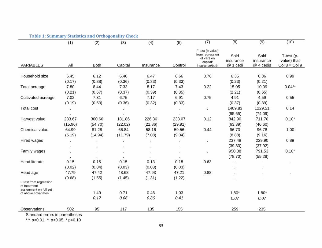
33
Table1:SummaryStatisticsandOrthogonalityCheck (1) (2) (3) (4) (5) (7) (8) (9) (10)
VARIABLES All Both Capital Insurance Control
F-test (p-value) from regression
of var1 on capital/
insurance/both
Sold
insurance @ 1 cedi
Sold insurance @ 4 cedis
T-test (p-value) that
Col 8 = Col 9 Household size 6.45 6.12 6.40 6.47 6.66 0.76 6.35 6.36 0.99
(0.17) (0.38) (0.36) (0.33) (0.33) (0.23) (0.21) Total acreage 7.80 8.44 7.33 8.17 7.43 0.22 15.05 10.09 0.04** (0.21) (0.67) (0.37) (0.39) (0.35) (2.21) (0.65) Cultivated acreage 7.02 7.31 6.75 7.17 6.91 0.75 4.91 4.59 0.55 (0.19) (0.53) (0.36) (0.32) (0.33) (0.37) (0.39) Total cost . . . . . . 1409.83 1229.51 0.14 . . . . . (95.65) (74.09) Harvest value 233.67 300.66 181.86 226.36 238.07 0.12 842.90 711.70 0.10* (15.96) (54.70) (22.02) (21.86) (29.91) (63.39) (46.60) Chemical value 64.99 81.28 66.84 58.16 59.56 0.44 96.73 96.78 1.00 (5.19) (14.94) (11.79) (7.08) (9.04) (8.88) (9.16) Hired wages . . . . . . 237.48 229.90 0.89 . . . . . (39.33) (37.92) Family wages . . . . . . 950.88 791.53 0.10* . . . . . (78.70) (55.28) Head literate 0.15 0.15 0.15 0.13 0.18 0.63 . . . (0.02) (0.04) (0.03) (0.03) (0.03) . . Head age 47.79 47.42 48.68 47.93 47.21 0.88 . . . (0.68) (1.55) (1.45) (1.31) (1.22) . . F-test from regression of treatment assignment on full set of above covariates 1.49 0.71 0.46 1.03 1.80* 1.80* 0.17 0.66 0.86 0.41 0.07 0.07 Observations 502 95 117 135 155 259 235
Standard errors in parentheses *** p<0.01, ** p<0.05, * p<0.10

34
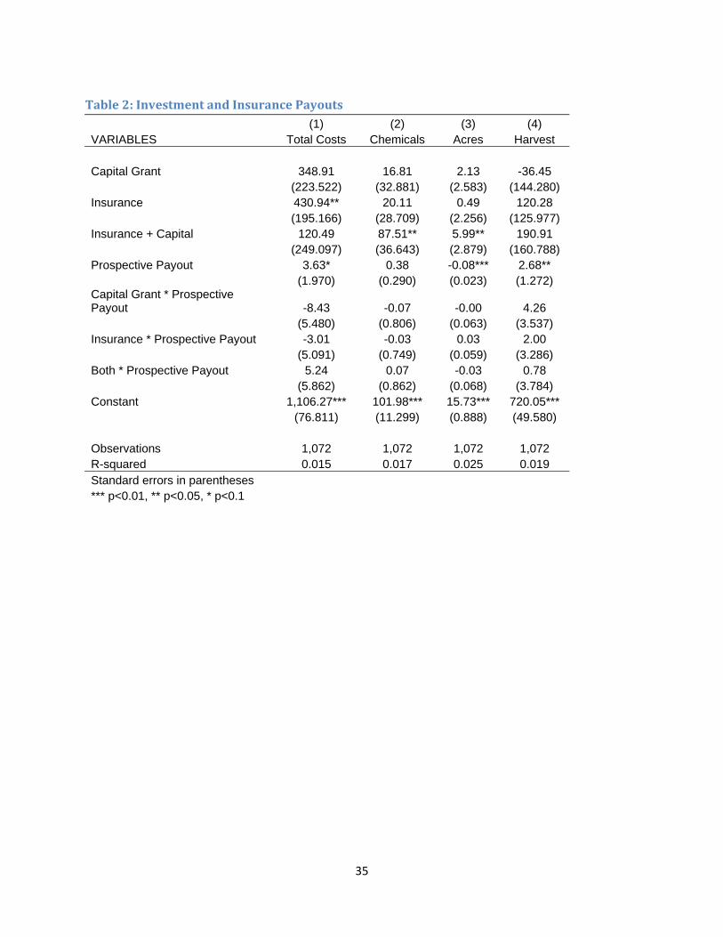
35
Table2:InvestmentandInsurancePayouts (1) (2) (3) (4) VARIABLES Total Costs Chemicals Acres Harvest Capital Grant 348.91 16.81 2.13 -36.45
(223.522) (32.881) (2.583) (144.280) Insurance 430.94** 20.11 0.49 120.28
(195.166) (28.709) (2.256) (125.977) Insurance + Capital 120.49 87.51** 5.99** 190.91
(249.097) (36.643) (2.879) (160.788) Prospective Payout 3.63* 0.38 -0.08*** 2.68**
(1.970) (0.290) (0.023) (1.272) Capital Grant * Prospective Payout -8.43 -0.07 -0.00 4.26
(5.480) (0.806) (0.063) (3.537) Insurance * Prospective Payout -3.01 -0.03 0.03 2.00
(5.091) (0.749) (0.059) (3.286) Both * Prospective Payout 5.24 0.07 -0.03 0.78
(5.862) (0.862) (0.068) (3.784) Constant 1,106.27*** 101.98*** 15.73*** 720.05***
(76.811) (11.299) (0.888) (49.580)
Observations 1,072 1,072 1,072 1,072 R-squared 0.015 0.017 0.025 0.019 Standard errors in parentheses *** p<0.01, ** p<0.05, * p<0.1
36
Table3:TheDemandforInsurance (1) (2) (3) (4)
VARIABLES Insurance Takeup
Insurance Takeup
Insurance Takeup
Insurance Takeup + Capital
Insurance Price (GHC) 0 0.98*** 1.00*** 1.00*** 0.00
(0.003) (0.001) (0.001) (0.000) 1 0.78*** 0.89*** 0.87*** 0.00
(0.021) (0.018) (0.018) (0.001) 3 0.65***
(0.026) 4 0.58*** 0.69*** 0.69*** 0.00
(0.028) (0.030) (0.029) (0.002) 6 0.56***
(0.028) 8 0.68*** 1.20*** 0.00
(0.086) (0.085) (0.002) 9 0.43***
(0.024) 9.5 0.64*** -0.05 1.16*** 0.00
(0.064) (0.102) (0.062) (0.002) 12 0.42*** -0.30*** 0.94*** 0.00
(0.070) (0.109) (0.068) (0.002) 14 0.31*** -0.39*** 0.83*** 0.00
(0.043) (0.090) (0.040) (0.002) Capital + Insurance at Price
0 0.98*** 1.00*** 1.00*** 1.00*** (0.003) (0.001) (0.001) (0.000)
1 0.81*** 0.89*** 0.88*** 0.88*** (0.029) (0.027) (0.028) (0.028)
3 0.71*** 0.78*** 0.78*** 0.78*** (0.039) (0.038) (0.038) (0.038)
Wealth at Baseline (/250 Cedis) 0.00
(0.001)
Observations 4,327 2,644 2,794 2,794 R-squared 0.564 0.746 0.737 0.869 Test additional demand with capital grant 4.451 Prob > F 0.0118 Notes: Year and year*sample stratification indicators included in all regressions. Samples: Column 1, years 1-3; columns 2-3 years 1-2. Linear probability model regressions, robust standard errors. F statistic in column 1 tests the hypothesis that the demand for insurance at prices 1 and 3 are equal with and without capital.
*** p<0.01, ** p<0.05, * p<0.1
37
Table4:IVEstimatesofEffectofInsuranceandCapitalGrantonInvestment
(1) (2) (3) (4) (5) (6) (7)
VARIABLES Total Costs Value of
Chemicals
Land Preparation
Cost Value of
Hired Labor Value of
Family Labor Cultivated
Acres Total Harvest Value Insured 254.14*** 31.87*** 22.37** 69.25* 116.69* 1.30*** 120.98**
(93.275) (10.383) (8.763) (38.827) (60.332) (0.423) (58.014) Insured+Grant 108.27 49.77*** 17.74* 33.86 -6.84 0.61 114.24**
(97.088) (11.032) (9.471) (42.969) (61.949) (0.446) (58.133) Grant 102.19 47.34*** 18.98** 65.32 -22.44 0.60 107.78*
(102.247) (12.114) (9.663) (45.537) (66.070) (0.475) (63.846) Constant 1,372.33*** 103.31*** 131.47*** 192.80*** 903.48*** 4.63*** 770.80***
(74.234) (8.685) (6.812) (32.325) (48.346) (0.319) (46.527)
Observations 2,794 2,794 2,794 2,794 2,794 2,794 2,794 R-squared 0.138 0.126 0.142 0.028 0.118 0.223 0.122 Median for Control 756 26 75 0 474.5 3 410 Notes: IV regressions with Insured & Insured + Grant treated as endogenous, with randomized prices as instruments. See Error! Reference source not found. columns 2 & 3 for first stage regressions. Year indicator and interactions with sample stratification indicators included but not reported. *** p<0.01, ** p<0.05, * p<0.1
38
Table5:InsuranceandtheRiskinessofProduction (1) (2) (3) (4) (5)
VARIABLES Total Harvest
Value Total Costs Value of
Chemicals Value of Hired
Labor Value of Hired
Labor Insured -660.58* -811.95 -146.75** -541.12** -94.92
(389.203) (627.824) (69.969) (263.636) (410.610) Insured + Grant 942.24* -616.54 74.62 194.67 -895.76
(554.089) (893.803) (99.612) (375.326) (584.565) Insured*Rainfall 105.25** 145.91* 23.49*** 81.96** 31.35
(49.640) (80.074) (8.924) (33.625) (52.370) (Insured+Grant)*Rain -107.81 91.97 -3.38 -21.72 114.28
(70.971) (114.483) (12.759) (48.074) (74.874) Grant -484.69 -661.93 -97.09 162.92 -811.02
(479.539) (773.546) (86.210) (324.828) (505.915) Grant*Rainfall 78.84 103.37 18.87* -11.13 104.47
(61.677) (99.492) (11.088) (41.779) (65.069) Rainfall (mm) 1,291.02*** 2,863.93*** 308.80*** 612.55** 1,907.14***
(407.276) (656.978) (73.218) (275.878) (429.677) Rainfall squared -83.68*** -188.77*** -20.04*** -37.73** -128.86***
(26.795) (43.223) (4.817) (18.150) (28.269) Constant -4,132.85*** -9,317.68*** -1,066.13*** -2,258.33** -6,019.01***
(1,523.430) (2,457.451) (273.876) (1,031.934) (1,607.222)
Observations 2,794 2,794 2,794 2,794 2,794 R-squared 0.130 0.148 0.140 0.042 0.128 Notes: IV regressions with Insured & Insured + Grant and their interactions with rainfall treated as endogenous, with randomized prices and prices interacted with rainfall as instruments. Year indicator and interactions with sample stratification indicators included but not reported. *** p<0.01, ** p<0.05, * p<0.1
39
Table6:HeterogeneityintheResponseofTotalCoststoTreatment (1) (2) (3) (4)
Interaction Variable: Non-land Wealth
Head Literate Head Age
Household Size
Insured 304.87*** 136.43 590.82*** 216.30
(94.885) (97.627) (221.821) (169.105) Insured + Grant 33.84 76.14 -32.54 22.99
(97.377) (104.276) (281.375) (211.756) Grant 153.33 -37.72 500.33* -30.34
(113.307) (120.518) (289.294) (225.747) Insured* interaction -0.17** 264.49* -7.92* 0.42
(0.070) (149.967) (4.519) (19.946) Both * interaction 0.09 -82.04 2.78 12.69
(0.079) (195.864) (5.901) (27.666) Grant * interaction -0.18** 204.87 -9.43 15.81
(0.085) (191.543) (6.046) (28.440) Interaction 0.26*** -7.66 5.71** 88.48***
(0.043) (73.620) (2.593) (11.147) Constant 1,290.39*** 1,458.72*** 1,169.02*** 777.87***
(78.329) (80.081) (139.237) (110.814)
Observations 2,644 2,570 2,164 2,176 R-squared 0.139 0.134 0.016 0.077 Notes: Dependent variable is total costs. IV regressions with Insured & Insured + Grant and their interactions with the interaction variable treated as endogenous, with randomized prices and prices interacted with the variable as instruments. Year indicator and interactions with sample stratification indicators included but not reported. *** p<0.01, ** p<0.05, * p<0.1
40
Table7:InvestmentandtheInsuranceMarket,TestingforSeparation
(1) (2) (3) (4) (5) (6) (7)
VARIABLES Total Costs Value of
Chemicals Value of Hired
Labor Value of
Family Labor
Land Preparation
Cost Cultivated
Area Harvest Value Insurance at Price
1 96.78 18.79 38.37 30.92 0.18 0.33 49.36 (118.582) (12.972) (48.088) (77.010) (11.040) (0.558) (71.685)
3 -196.11 -11.94 -25.59 -93.56 -33.21*** -1.43** -157.11** (123.593) (13.520) (50.121) (80.265) (11.506) (0.582) (74.715)
Insurance at Price and Grant
1 317.68** 67.51*** 63.44 131.96 29.32** 1.42** 280.76*** (144.665) (15.825) (58.666) (93.950) (13.468) (0.681) (87.454)
3 126.29 31.97* 34.46 54.66 -10.84 -0.07 -17.38 (152.739) (16.708) (61.940) (99.193) (14.220) (0.719) (92.335)
Constant 1,500.96*** 127.70*** 230.84*** 916.30*** 150.02*** 8.88*** 861.41*** (93.922) (10.274) (38.088) (60.996) (8.744) (0.442) (56.778)
Observations 1,397 1,397 1,397 1,397 1,397 1,397 1,397 R-squared 0.023 0.042 0.011 0.018 0.042 0.025 0.036 Test additional investment with capital grant 3.886 9.559 0.633 1.940 4.201 3.545 5.497 Prob > F 0.0208 7.53e-05 0.531 0.144 0.0152 0.0291 0.00419 Notes: Prices higher than 3 cedis, year indicator, and interactions of year with sample stratification indicators included but not reported. . F statistic in bottom row tests the hypothesis that the investment at prices 1 and 3 are equal with and without capital *** p<0.01, ** p<0.05, * p<0.1
41
Table8:Experience,SocialInteractionsandtheDemandforInsurance (1) (2) (3) (4) (5) (6) Network: Credit Family Relationship Farm Information Insurance variable: Acres Insured Takeup Acres Insured Takeup Acres Insured Takeup Insured, with payout last year 2.20*** 0.16*** 1.82*** 0.13*** 1.84*** 0.14***
(0.238) (0.029) (0.253) (0.031) (0.254) (0.032) Insured, w/o payout last year -0.59** -0.16*** -0.52** -0.15*** -0.53** -0.16***
(0.240) (0.030) (0.236) (0.030) (0.236) (0.030) SN Share insured, w/payout last year 1.61*** 0.13** 1.80*** 0.18*** 1.16*** 0.15***
(0.445) (0.054) (0.393) (0.049) (0.382) (0.048) SN Share insured, w/o payout last year -0.23 -0.04 -0.27 0.02 -0.77** 0.02
(0.367) (0.045) (0.331) (0.041) (0.311) (0.039) SN Share Capital last year 1.30* 0.09 2.03*** 0.21*** 0.82 0.18**
(0.667) (0.081) (0.633) (0.078) (0.635) (0.079) Number in SN 0.02 0.00 0.04*** 0.00 0.04** -0.00
(0.017) (0.002) (0.014) (0.002) (0.017) (0.002) Insurance Price -0.31*** -0.04*** -0.31*** -0.04*** -0.31*** -0.04***
(0.027) (0.003) (0.027) (0.003) (0.027) (0.004) Observations 2,202 2,122 2,202 2,122 2,202 2,122 R-squared 0.340 0.283 0.366 0.288 0.367 0.276 Notes: IV regressions with own insurance with and without payout instrumented by prices last year, interacted with rainfall triggers for insurance. SN Share insured with and without payouts instrumented by the shares of the SN offered different prices last year, interacted with rainfall triggers. Year indicators, interactions with sample stratification indicators, number of respondents in community included but not reported. Mean acres insured is 5.5, mean takeup is 62%. *** p<0.01, ** p<0.05, * p<0.1
42
Table9:RecencyBias,TrustandtheDemandforInsurance (1) (2) (3) (4) (5) (6) Network: Credit Family Relationship Farm Information Insurance variable: Acres Insured Takeup Acres Insured Takeup Acres Insured Takeup Insured, with payout last year 1.79*** 0.12*** 1.61*** 0.11*** 1.62*** 0.12***
(0.245) (0.030) (0.254) (0.032) (0.255) (0.032) Insured, w/o payout last year -0.51** -0.15*** -0.49** -0.15*** -0.50** -0.15***
(0.239) (0.029) (0.235) (0.030) (0.234) (0.030) Prospective Payout last year 1.07*** 0.10*** 1.01*** 0.10*** 1.03*** 0.10***
(0.179) (0.022) (0.179) (0.023) (0.177) (0.023) SN Share insured, w/payout last year 1.45*** 0.11** 1.46*** 0.15*** 0.74* 0.11**
(0.443) (0.054) (0.396) (0.049) (0.385) (0.048) SN Share insured, w/o payout last year -0.04 -0.02 0.14 0.05 -0.42 0.05
(0.369) (0.045) (0.336) (0.042) (0.315) (0.039) SN Share Capital last year 1.31** 0.09 2.03*** 0.21*** 0.77 0.18**
(0.662) (0.081) (0.628) (0.078) (0.630) (0.079) Number in SN 0.01 -0.00 0.03** 0.00 0.03* -0.00
(0.017) (0.002) (0.014) (0.002) (0.017) (0.002) Insurance Price -0.30*** -0.04*** -0.29*** -0.04*** -0.29*** -0.04***
(0.027) (0.003) (0.027) (0.003) (0.027) (0.004) Observations 2,202 2,122 2,202 2,122 2,202 2,122 R-squared 0.340 0.283 0.366 0.288 0.367 0.276 Notes: IV regressions with own insurance with and without payout instrumented by prices last year, interacted with rainfall triggers for insurance. SN Share insured with and without payouts instrumented by the shares of the SN offered different prices last year, interacted with rainfall triggers. Year indicators, interactions with sample stratification indicators, number of respondents in community included but not reported. Mean acres insured is 5.5, mean takeup is 62%. *** p<0.01, ** p<0.05, * p<0.1
43
AppendixTable1:HomesteadtoRainfallGaugeDistanceSummaryStatisticsin2009&2010
(1) (2) (3) (4) (5)
GAUGE Mean Standard Deviation
Number of Farmers
2009 Mean Rainfall Amount
2010 Mean Rainfall Amount
Savelugu 8.364 7.146 264 6.740 ‐ Tamale Old Airport 6.689 3.559
171 7.020 ‐
Pong Tamale 11.979 6.417
392 6.115 6.050
Tamale Airport 13.365 7.639
469 7.439 5.966
Walewale 32.765 8.382
389 5.175 5.598
44
Figure1:EffectofInsuranceandCashGrantsonTotalInvestment
0.2
.4.6
.81
0 1000 2000 3000 4000 5000Total Costs (Cedis)
Control Insurance
CDF of Total Costs
0.2
.4.6
.81
0 1000 2000 3000 4000Total Costs (Cedis)
Control Capital
CDF of Total Costs0
.2.4
.6.8
1
0 1000 2000 3000 4000Total Costs (Cedis)
Control Both
CDF of Total Costs
45
Figure2:EffectofInsuranceandCashGrantsonChemicalExpenditure
.2.4
.6.8
1
0 100 200 300 400Value of Agricultural Chemicals (Cedis)
Control Insurance
CDF of Chemicals Applied
.2.4
.6.8
1
0 100 200 300 400Value of Agricultural Chemicals (Cedis)
Control Capital
CDF of Chemicals Applied0
.2.4
.6.8
1
0 200 400 600 800Value of Agricultural Chemicals (Cedis)
Control Both
CDF of Chemicals Applied
46
Figure3:EffectofInsuranceandCashGrantsonAreaCultivated
.2.4
.6.8
1
0 5 10 15Total Acres Cultivated
Control Insurance
CDF of Cultivated Acres
.2.4
.6.8
1
0 5 10 15Total Acres Cultivated
Control Capital
CDF of Cultivated Acres.2
.4.6
.81
0 5 10 15 20Total Acres Cultivated
Control Both
CDF of Cultivated Acres
47
Figure4:EffectofInsuranceandCashGrantsonValueofHarvest
0.2
.4.6
.81
0 1000 2000 3000Value of Harvest (Cedis)
Control Insurance
CDF of Harvest
0.2
.4.6
.81
0 500 1000 1500 2000 2500Value of Harvest (Cedis)
Control Capital
CDF of Harvest0
.2.4
.6.8
1
0 500 1000 1500 2000 2500Value of Harvest (Cedis)
Control Both
CDF of Harvest
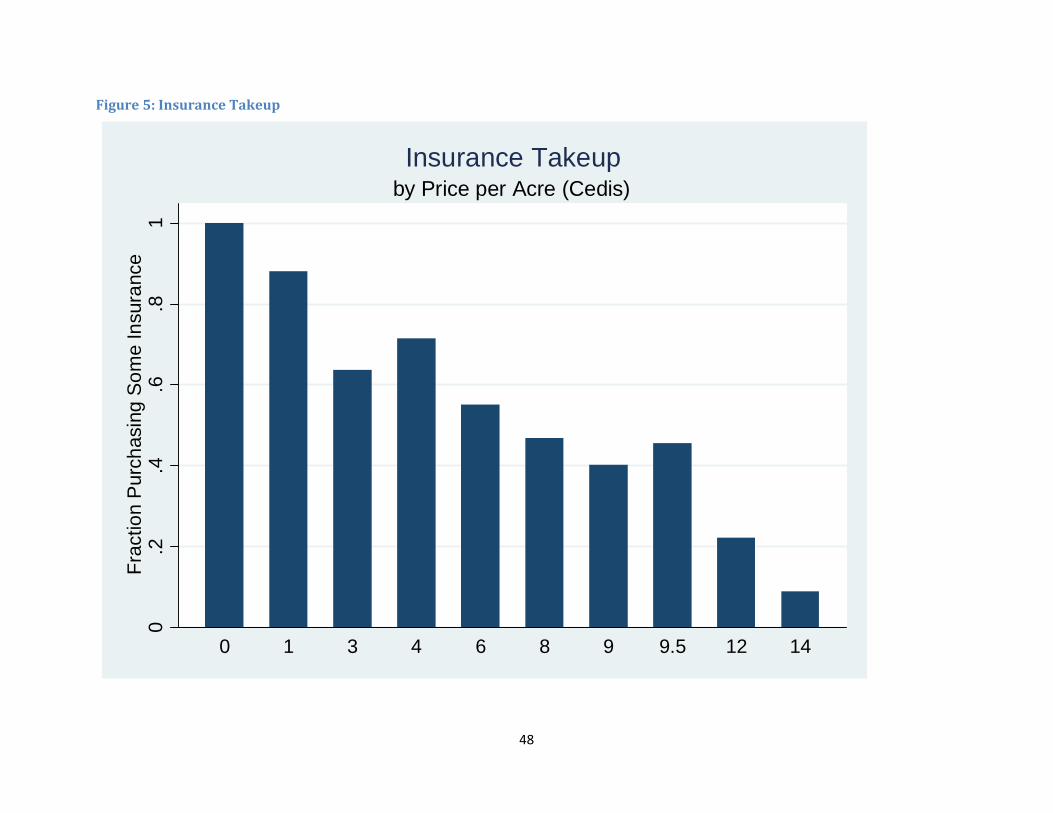
48
Figure5:InsuranceTakeup
0.2
.4.6
.81
Frac
tion
Pur
chas
ing
Som
e In
sura
nce
0 1 3 4 6 8 9 9.5 12 14
by Price per Acre (Cedis)Insurance Takeup
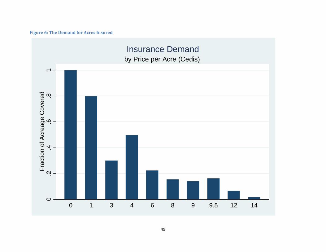
49
Figure6:TheDemandforAcresInsured
0.2
.4.6
.81
Frac
tion
of A
crea
ge C
over
ed
0 1 3 4 6 8 9 9.5 12 14
by Price per Acre (Cedis)Insurance Demand
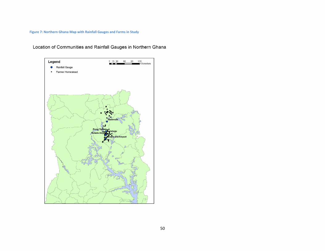
50
Figure 7: Northern Ghana Map with Rainfall Gauges and Farms in Study