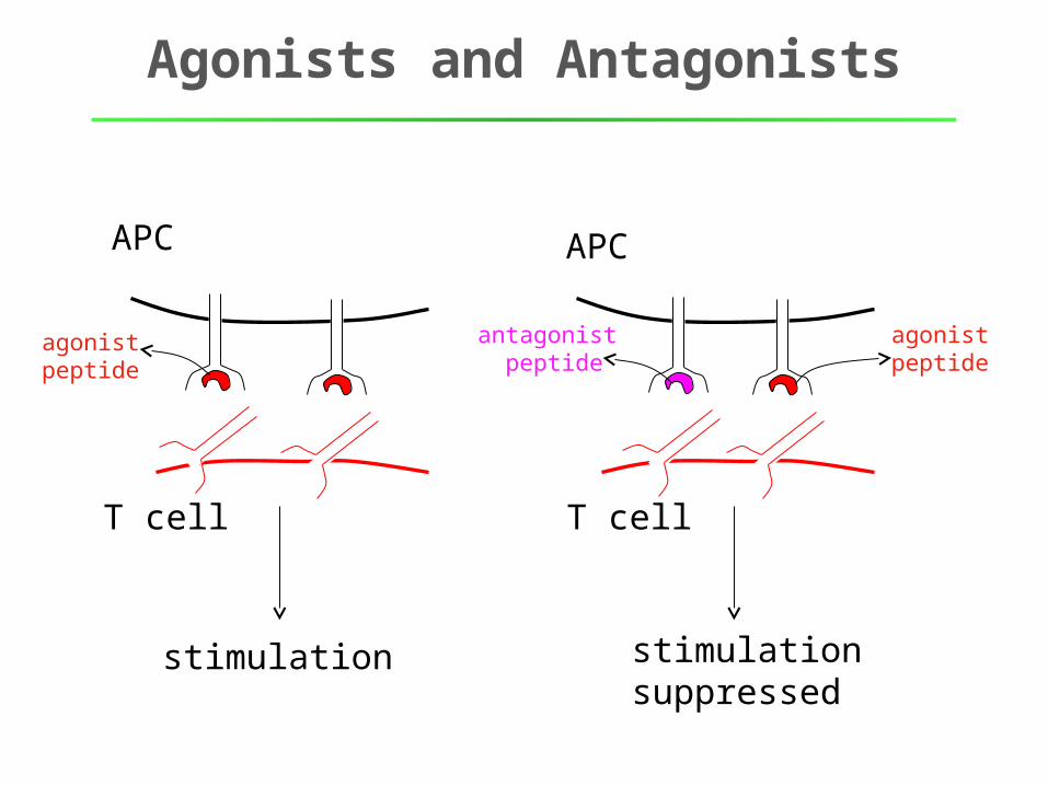
Agonists and Antagonists

APC

T cell

agonistpeptide

APC

T cell

antagonist peptide

agonistpeptide

stimulation stimulationsuppressed

Agonists and Antagonists

APC

T cell

agonistpeptide

agonistpeptide

stimulation stimulationsuppressed

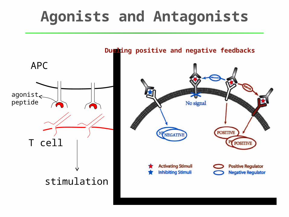
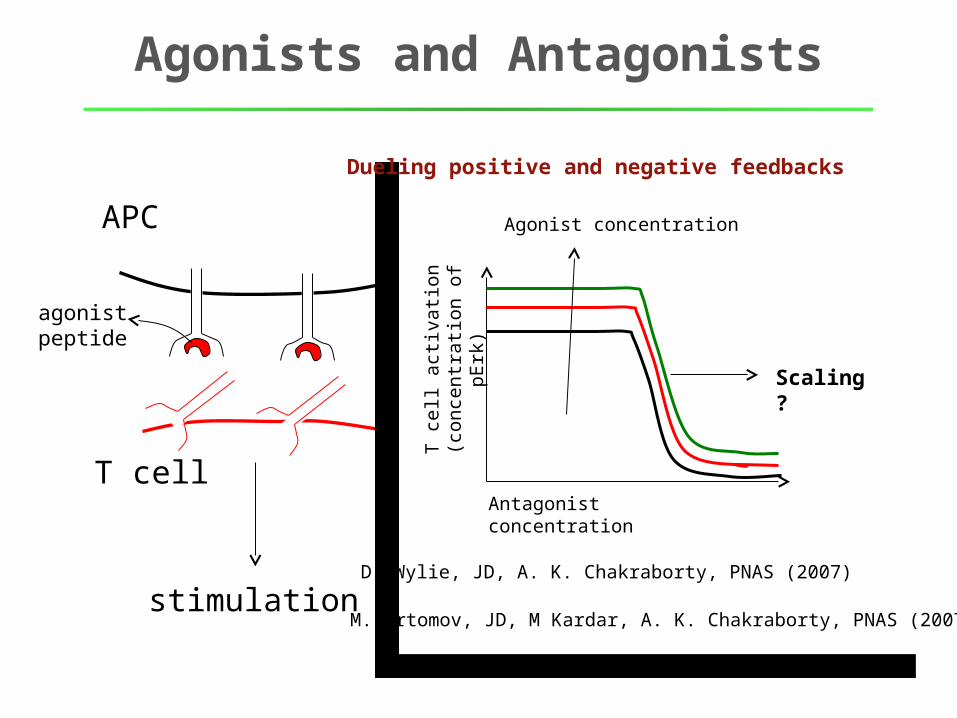
Dueling positive and negative feedbacks

Agonists and Antagonists

APC

T cell

APC

agonistpeptide

stimulation stimulationsuppressed

Dueling positive and negative feedbacks

T c

ell a

ctiv

atio

n(c

once

ntra

tion

of p

Erk

)

Antagonist concentration

Scaling ?

Agonist concentration

D. Wylie, JD, A. K. Chakraborty, PNAS (2007)

M. Artomov, JD, M Kardar, A. K. Chakraborty, PNAS (2007)

+ve

-ve

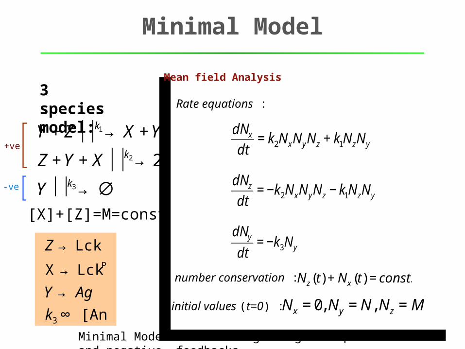
Minimal Model

€

Y + Z k1 ⏐ → ⏐ X + Y

Z + Y + X k2 ⏐ → ⏐ 2X + Y

Y k3 ⏐ → ⏐ ∅

• Irreversibility• Branching• Feedback with distinct time scale

3 species model:

€

Z → Lck

X → LckP

Y → Ag

k3 ∞ [Ant]

Minimal Model for cell signaling with positive and negative feedbacks

[X]+[Z]=M=const

+ve

-ve

Minimal Model

€

Y + Z k1 ⏐ → ⏐ X + Y

Z + Y + X k2 ⏐ → ⏐ 2X + Y

Y k3 ⏐ → ⏐ ∅

• Irreversibility• Branching• Feedback with distinct time scale

3 species model:

€

Z → Lck

X → LckP

Y → Ag

k3 ∞ [Ant]

Minimal Model for cell signaling with positive and negative feedbacks

[X]+[Z]=M=const €

dNx

dt= k2NxNyNz + k1NzNy

€

dNz

dt= −k2NxNyNz − k1NzNy

€

dNy

dt= −k3Ny

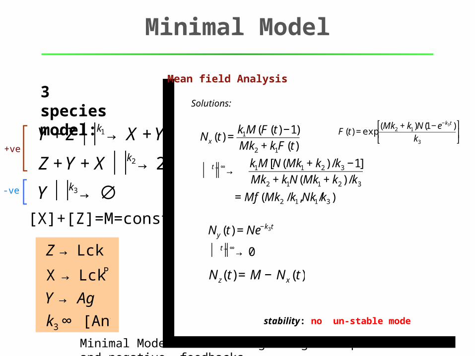
Mean field Analysis

€

Nx = 0, Ny = N, Nz = Minitial values (t=0) :

Rate equations :

€

Nz(t) + Nx (t) = const.number conservation :

+ve

-ve

Minimal Model

€

Y + Z k1 ⏐ → ⏐ X + Y

Z + Y + X k2 ⏐ → ⏐ 2X + Y

Y k3 ⏐ → ⏐ ∅

• Irreversibility• Branching• Feedback with distinct time scale

3 species model:

€

Z → Lck

X → LckP

Y → Ag

k3 ∞ [Ant]

Minimal Model for cell signaling with positive and negative feedbacks

[X]+[Z]=M=const

€

Nx (t) =k1M(F(t) −1)

Mk2 + k1F(t)

t →∞ ⏐ → ⏐ ⏐ k1M[N(Mk1 + k2) /k3 −1]

Mk2 + k1N(Mk1 + k2) /k3

= Mf (Mk2 /k1,Nk1/k3)

€

Ny (t) = Ne−k3t

t →∞ ⏐ → ⏐ ⏐ 0

€

N z( t) = M − N x(t)

€

F(t) = exp(Mk2 + k1)N(1− e−k3t )

k3

⎡

⎣ ⎢

⎤

⎦ ⎥

stability: no un-stable mode

Mean field Analysis

Solutions:

+ve

-ve

Minimal Model

€

Y + Z k1 ⏐ → ⏐ X + Y

Z + Y + X k2 ⏐ → ⏐ 2X + Y

Y k3 ⏐ → ⏐ ∅

• Irreversibility• Branching• Feedback with distinct time scale

3 species model:

€

Z → Lck

X → LckP

Y → Ag

k3 ∞ [Ant]

Minimal Model for cell signaling with positive and negative feedbacks

[X]+[Z]=M=const

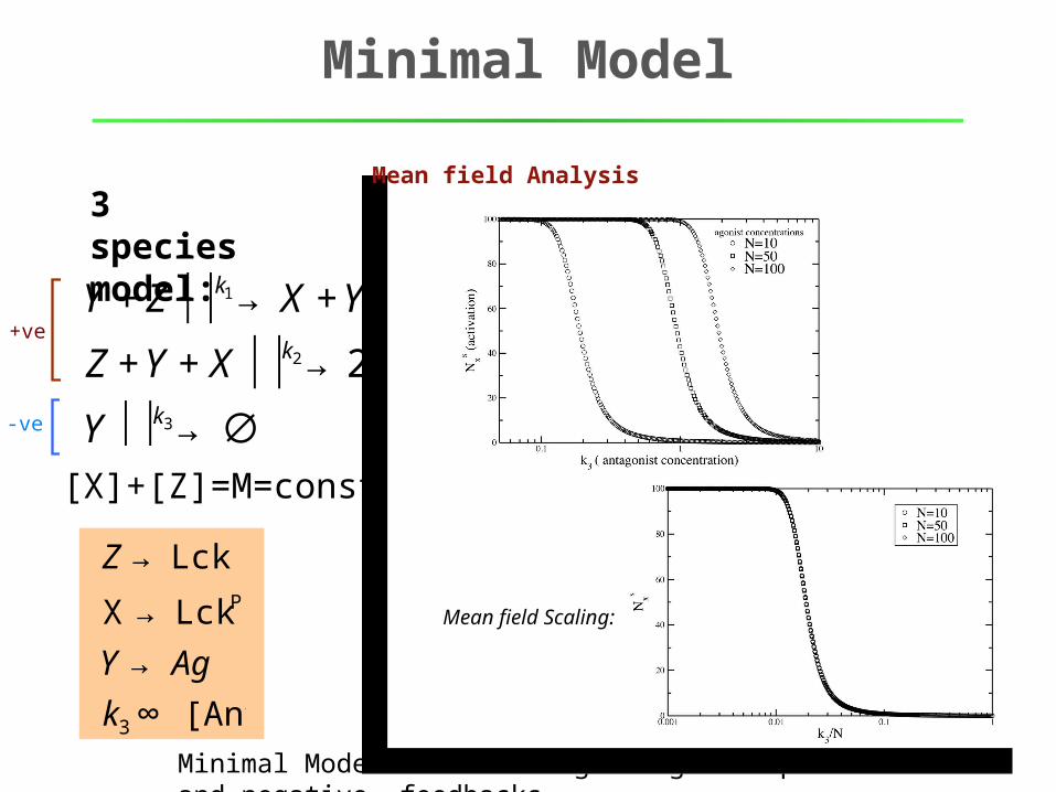
Mean field Analysis

Mean field Scaling:

+ve

-ve

Minimal Model

€

Y + Z k1 ⏐ → ⏐ X + Y

Z + Y + X k2 ⏐ → ⏐ 2X + Y

Y k3 ⏐ → ⏐ ∅

• Irreversibility• Branching• Feedback with distinct time scale

3 species model:

€

Z → Lck

X → LckP

Y → Ag

k3 ∞ [Ant]

Minimal Model for cell signaling with positive and negative feedbacks

[X]+[Z]=M=const

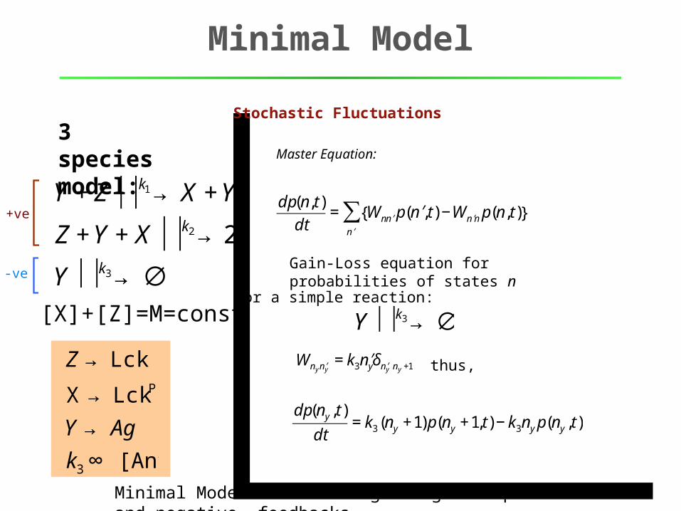
Stochastic Fluctuations

€

dp(n, t)

dt= Wn ′ n p( ′ n , t) −W ′ n n p(n, t){ }

′ n

∑

Master Equation:

Gain-Loss equation for probabilities of states n

€

Y k3 ⏐ → ⏐ ∅For a simple reaction:

€

dp(ny, t)

dt= k3(ny +1)p(ny +1, t) − k3ny p(ny, t)€

Wny ′ n y= k3 ′ n yδ ′ n y ny +1 thus,

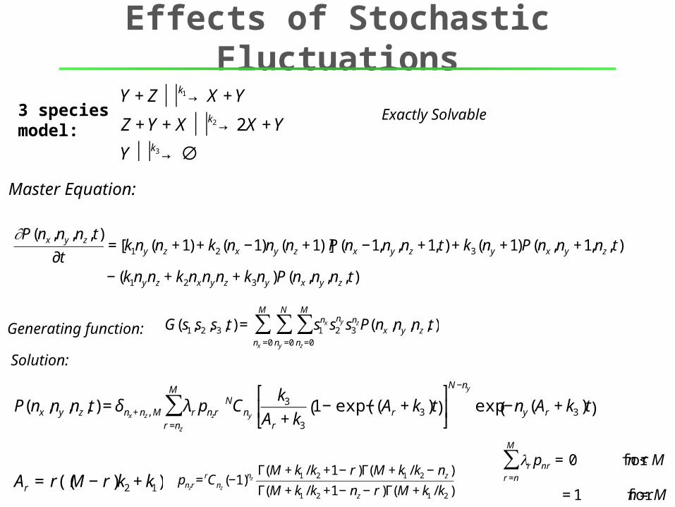
Effects of Stochastic Fluctuations

€

∂P(nx,ny,nz, t)

∂t= [k1ny (nz +1) + k2(nx −1)ny (nz +1)]P(nx −1,ny,nz +1, t) + k3(ny +1)P(nx,ny +1,nz, t)

− (k1nynz + k2nxnynz + k3ny )P(nx,ny,nz, t)

Master Equation:

Exactly Solvable

€

Y + Z k1 ⏐ → ⏐ X + Y

Z + Y + X k2 ⏐ → ⏐ 2X + Y

Y k3 ⏐ → ⏐ ∅

3 species model:

€

G(s1,s2 ,s3 ,t) = s1nx s2

ny s3nz

nz =0

M

∑ny =0

N

∑nx =0

M

∑ P(nx ,ny ,nz ,t)Generating function:

€

P(nx ,ny ,nz ,t) = δnx + nz, M λrr =nz

M

∑ pnzrNCny

k3

Ar + k3

1− exp(−(Ar + k3 )t( ) ⎡

⎣ ⎢

⎤

⎦ ⎥

N −ny

exp −ny(Ar + k3 )t( )

€

Ar = r((M − r )k2 + k1)

€

pnzr= rCnz

(−1)nzΓ(M + k1 / k2 +1− r )Γ(M + k1 / k2 − nz )

Γ(M + k1 / k2 +1− nz − r )Γ(M + k1 / k2 )

€

λr pnrr =n

M

∑ = 0 for n < M

= 1 for n = M

Solution:

Effects of Stochastic Fluctuations

€

∂P(nx,ny,nz, t)

∂t= [k1ny (nz +1) + k2(nx −1)ny (nz +1)]P(nx −1,ny,nz +1, t) + k3(ny +1)P(nx,ny +1,nz, t)

− (k1nynz + k2nxnynz + k3ny )P(nx,ny,nz, t)

Master Equation:

Exactly Solvable

€

Y + Z k1 ⏐ → ⏐ X + Y

Z + Y + X k2 ⏐ → ⏐ 2X + Y

Y k3 ⏐ → ⏐ ∅

3 species model:

€

G(s1,s2 ,s3 ,t) = s1nx s2

ny s3nz

nz =0

M

∑ny =0

N

∑nx =0

M

∑ P(nx ,ny ,nz ,t)

€

P(nx ,ny ,nz ,t) = δnx + nz, M λrr =nz

M

∑ pnzrNCny

k3

Ar + k3

1− exp(−(Ar + k3 )t( ) ⎡

⎣ ⎢

⎤

⎦ ⎥

N −ny

exp −ny(Ar + k3 )t( )

€

Ar = r((M − r )k2 + k1)

€

pnzr= rCnz

(−1)nzΓ(M + k1 / k2 +1− r )Γ(M + k1 / k2 − nz )

Γ(M + k1 / k2 +1− nz − r )Γ(M + k1 / k2 )

€

λr pnrr =n

M

∑ = 0 for n < M

= 1 for n = M

Generating function:

Solution:

[X]+[Z]=M=const

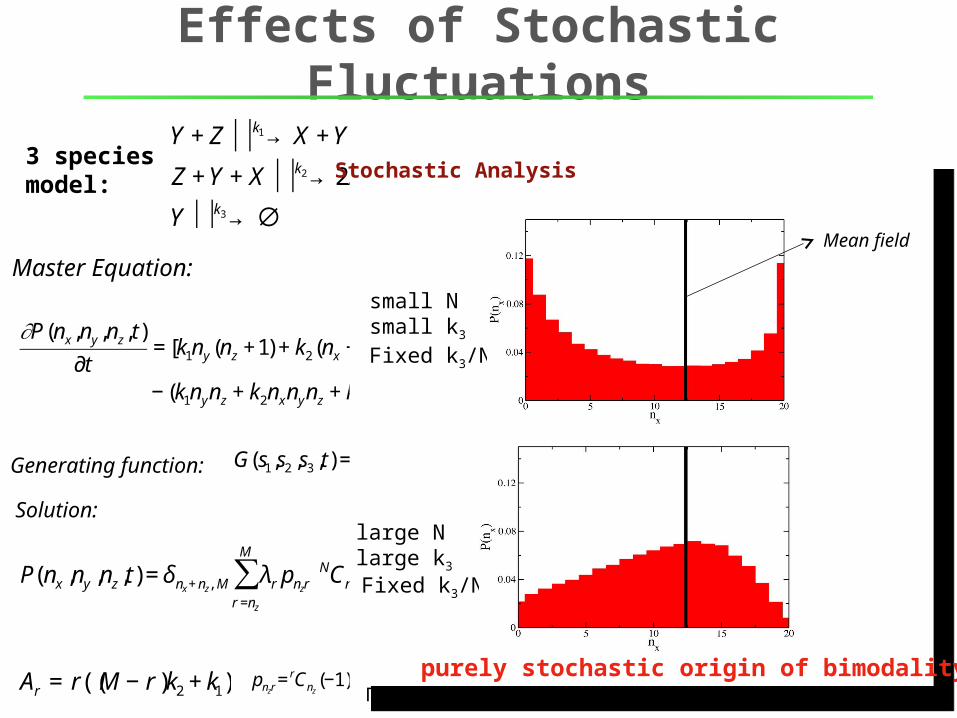
small Nsmall k3

Fixed k3/N

Stochastic Analysis

Mean field

large Nlarge k3

Fixed k3/N

purely stochastic origin of bimodality

Effects of Stochastic Fluctuations

€

∂P(nx,ny,nz, t)

∂t= [k1ny (nz +1) + k2(nx −1)ny (nz +1)]P(nx −1,ny,nz +1, t) + k3(ny +1)P(nx,ny +1,nz, t)

− (k1nynz + k2nxnynz + k3ny )P(nx,ny,nz, t)

Master Equation:

Exactly Solvable

€

Y + Z k1 ⏐ → ⏐ X + Y

Z + Y + X k2 ⏐ → ⏐ 2X + Y

Y k3 ⏐ → ⏐ ∅

3 species model:

€

G(s1,s2 ,s3 ,t) = s1nx s2

ny s3nz

nz =0

M

∑ny =0

N

∑nx =0

M

∑ P(nx ,ny ,nz ,t)

€

P(nx ,ny ,nz ,t) = δnx + nz, M λrr =nz

M

∑ pnzrNCny

k3

Ar + k3

1− exp(−(Ar + k3 )t( ) ⎡

⎣ ⎢

⎤

⎦ ⎥

N −ny

exp −ny(Ar + k3 )t( )

€

Ar = r((M − r )k2 + k1)

€

pnzr= rCnz

(−1)nzΓ(M + k1 / k2 +1− r )Γ(M + k1 / k2 − nz )

Γ(M + k1 / k2 +1− nz − r )Γ(M + k1 / k2 )

€

λr pnrr =n

M

∑ = 0 for n < M

= 1 for n = M

Generating function:

Solution:

[X]+[Z]=M=const

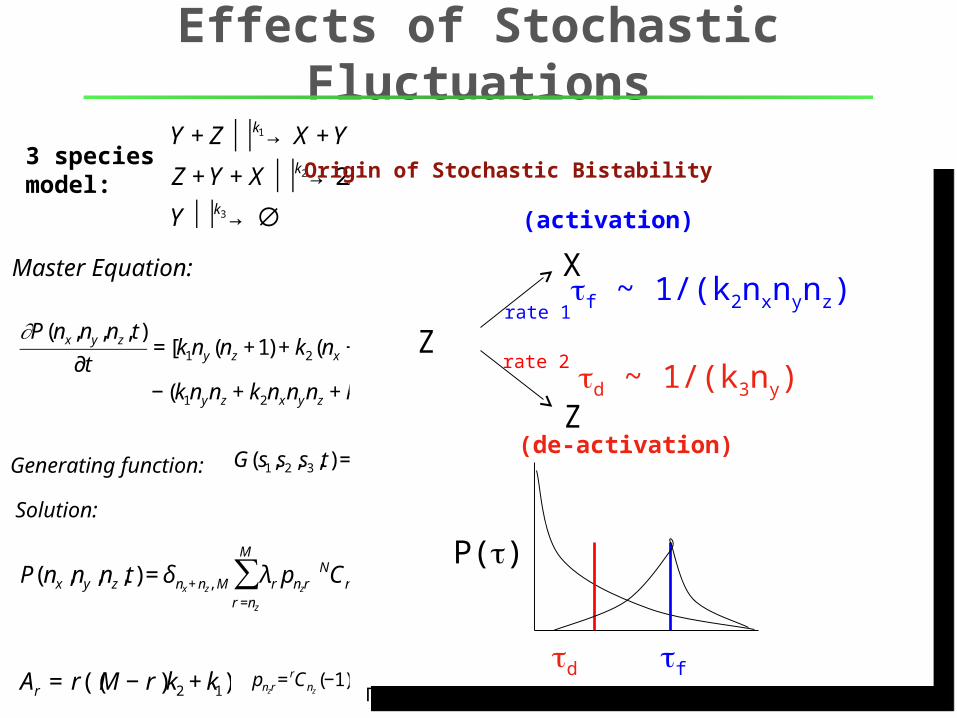
Origin of Stochastic Bistability

Z

X

rate 2

rate 1

Zd ~ 1/(k3ny)

f ~ 1/(k2nxnynz)

fd

P()

(activation)

(de-activation)

Effects of Stochastic Fluctuations

€

∂P(nx,ny,nz, t)

∂t= [k1ny (nz +1) + k2(nx −1)ny (nz +1)]P(nx −1,ny,nz +1, t) + k3(ny +1)P(nx,ny +1,nz, t)

− (k1nynz + k2nxnynz + k3ny )P(nx,ny,nz, t)

Master Equation:

€

Y + Z k1 ⏐ → ⏐ X + Y

Z + Y + X k2 ⏐ → ⏐ 2X + Y

Y k3 ⏐ → ⏐ ∅

3 species model:

€

P(nx ,ny ,nz ,t) = δnx + nz, M λrr =nz

M

∑ pnzrNCny

k3

Ar + k3

1− exp(−(Ar + k3 )t( ) ⎡

⎣ ⎢

⎤

⎦ ⎥

N −ny

exp −ny(Ar + k3 )t( )

€

Ar = r((M − r )k2 + k1)

€

pnzr= rCnz

(−1)nzΓ(M + k1 / k2 +1− r )Γ(M + k1 / k2 − nz )

Γ(M + k1 / k2 +1− nz − r )Γ(M + k1 / k2 )

€

λr pnrr =n

M

∑ = 0 for n < M

= 1 for n = M

Generating function:

Solution:

fd

P()

fd

P()

reduction of

ny and k3

fd

P()

fd

P()

reduction of

ny and k3

time, arbitrary units

reac

tion

rate

s

2 4 6 8 10

0.25

0.5

0.75

1

1.25

1.5

1.75

2

discrete partic

le numberstochasticfluctuations

[X]+[Z]=M=const

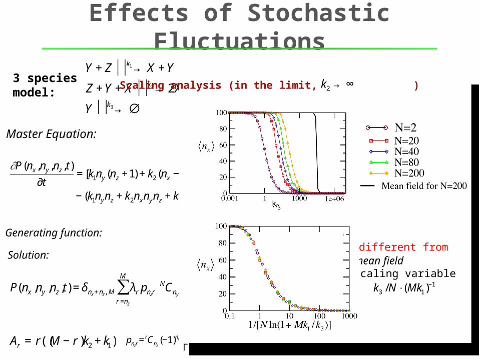
Scaling analysis (in the limit, )

k3

mean field scaling variable

€

k3 /N ⋅(Mk1)−1

different from

€

k2 → ∞

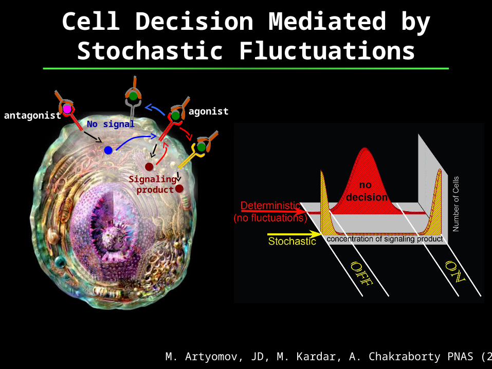
Cell Decision Mediated by Stochastic Fluctuations

agonistantagonist

Signaling product

No signal

M. Artyomov, JD, M. Kardar, A. Chakraborty PNAS (2007)