AGN at 1-­‐100 MeV

Jus0n Finke Naval Research Laboratory

13 November 2015

1

•  Thanks to: – Roopesh Ojha – Greg Madejeski – Abe Falcone – Teddy Cheung

•  Opinions and mistakes are mine alone

17"

AdEPT,

Fermi,LAT,COMPAIR,

Alex"Moiseev""""Future"Space4based"Gamma4ray"observa:ons"""Feb"6,"2015"

GSFC"

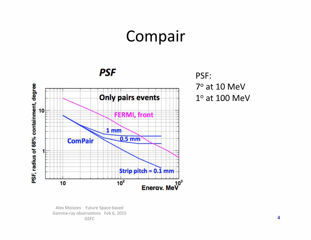
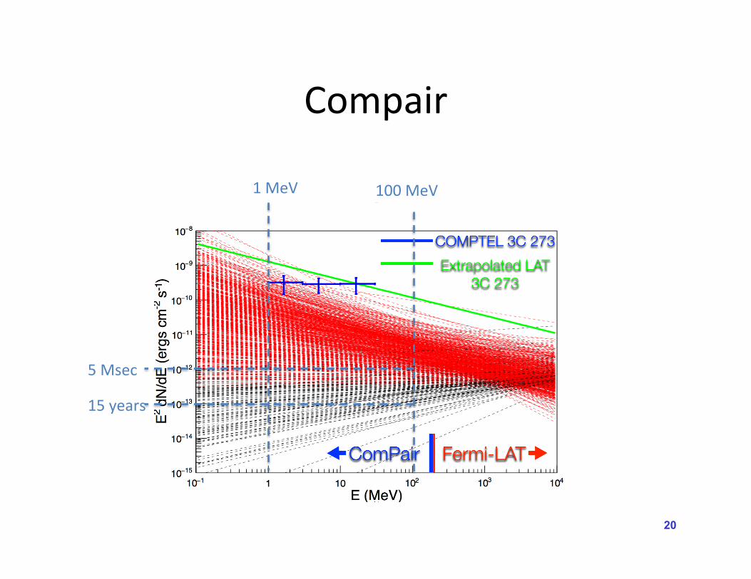
Compair

3

15"

Instrument,Response,Func0ons,

Alex"Moiseev""""Future"Space4based"Gamma4ray"observa:ons"""Feb"6,"2015"

GSFC"

15"

Instrument,Response,Func0ons,

Alex"Moiseev""""Future"Space4based"Gamma4ray"observa:ons"""Feb"6,"2015"

GSFC" 4

PSF: 7o at 10 MeV 1o at 100 MeV

Compair

1-­‐100 MeV Telescope •  Assume 10-­‐12 erg cm-­‐2 s-­‐1 in ~1 Msec (11.5 days) and flux sensi0vity goes as sqrt(0me)

•  It will reach 10-­‐13 erg cm-­‐2 s-­‐1 in ~3 years. •  Will it be wide field of view instrument like Fermi? Mul0ply 0mescales by 5

17"

AdEPT,

Fermi,LAT,COMPAIR,

Alex"Moiseev""""Future"Space4based"Gamma4ray"observa:ons"""Feb"6,"2015"

GSFC" 5

Compare with COMPTEL which reached ~ 10-­‐10 erg cm-­‐2 s-­‐1

COMPTEL New Blazar Detections at MeV Energies by COMPTEL 123

Table 1. Updated list of COMPTEL AGN detections. Apart from the fournew sources and Mkn 421 (Collmar et al. 1999), all others are listed in thefirst COMPTEL source catalog. The table lists the source name, the redshift,the AGN type, and a qualitative statement on the COMPTEL detection sig-nificance.

Source Redshift AGN Type SignificanceCen A 0.0007 radio galaxy highMkn 421 0.031 BL Lac object low3C 273 0.158 quasar highPKS 1222+216 0.435 quasar medium3C 279 0.538 quasar highPKS 1622-297 0.815 quasar high3C 454.3 0.859 quasar highPKS 0208-512 1.003 quasar highCTA 102 1.037 quasar lowGRO J0516-609 1.09 quasar mediumPKS 1127-145 1.187 quasar mediumPKS 0528+134 2.06 quasar highPKS 0716+714 ? BL Lac object low0836+710 2.17 quasar mediumPKS 1830-210 2.06 quasar medium

EGRET-detected blazars on the basis of positional and spectral coincidence:PKS 1830-210, PKS 1127-145, 0836+710, and PKS 0716+714. These objectsare added to the list of AGN detected by COMPTEL, incrementing this list to15 objects (Table 1). Three of the four new sources are quasar-type blazars withsteep γ-ray spectra in the EGRET band. We found that these spectra continueinto the COMPTEL band, where they seem to change their slope towards aharder spectrum. This indicates that for these sources the peak of the inverse-Compton emission is at MeV energies, similar to several other such objects likePKS 0528+134 for example (Collmar et al. 1997). Due to the low detection sig-nificance, the case for PKS 0716+714 is less clear. PKS 0716+714 is the secondBL Lac object for which evidence is found in the COMPTEL data, although inboth cases on a weak significance level (Table 1).

References

B!lazejowski, M., Siemiginowska, A., Sikora, M., et al. 2004, ApJ 600, L27Collmar, W., Bennett, K., Bloemen, H., et al. 1997, A&A 328, 33Collmar, W., Bennett, K., Bloemen, H., et al. 1999, Proc. of the 36th ICRC, Salt Lake

City, USA; eds. D.Kieda, M. Salamon, B. Dingus, Vol. 3, 374Hartman, R.C., Bertsch, D.L., Bloom, S.D., et al. 1999, ApJS 123, 79Lidman, C., Courbin F., Meylan, G., et al. 1999, ApJ 514, L57Schonfelder, V., Bennett, K., Blom, J.J., et al. 2000, A&AS 143, 145

6

COMPTEL saw 15 AGN radio loud AGN and 0 radio quiet AGN (Collmar 2006)

Collmar (2006)

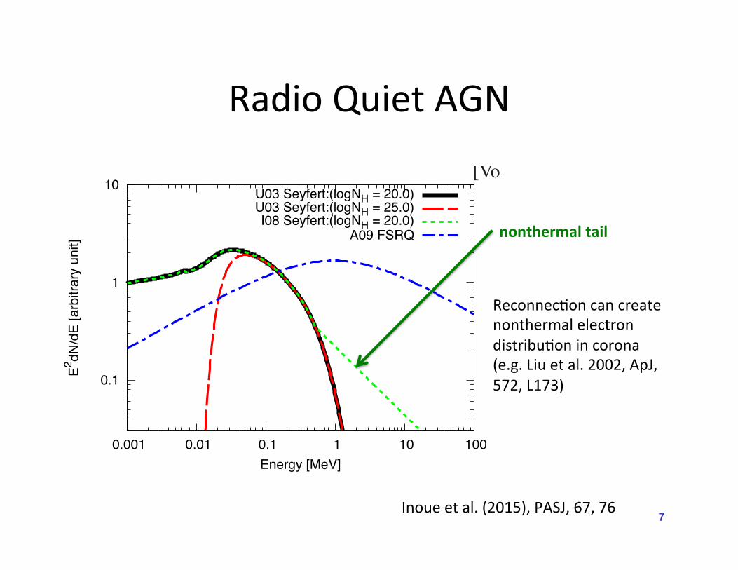
Radio Quiet AGN

7

2 [Vol. ,

ground spectrum is smoothly connected to the CXB spectrumand shows softer (photon index of Γ∼ 2.8 Fukada et al., 1975;Watanabe et al., 1997; Weidenspointner et al., 2000) than theGeV component (photon index of Γ ∼ 2.4 Ackermann et al.,2015a), indicating their different origins.Several candidates have been considered as the origin of the

MeV background. One was the nuclear-decay gamma raysfrom Type Ia supernovae (Clayton & Ward, 1975; Zdziarski,1996; Watanabe et al., 1999). However, the measurementsof the cosmic Type Ia supernovae rates show that the ratesare not enough to explain the observed flux (e.g. Ahn et al.,2005; Strigari et al., 2005; Horiuchi & Beacom, 2010; Ruiz-Lapuente et al., 2015). Seyferts may naturally explain theMeV background up to a few tens of MeV and the smoothconnection to the CXB (Schoenfelder, 1978; Field & Rogers,1993; Stecker et al., 1999; Inoue et al., 2008, hereinafter I08).Non-thermal electrons in coronae can generate the power-lawspectrum in the MeV band after the thermal cut-off via theCompton scattering of disk photons (I08). Flat-spectrum ra-dio quasars (FSRQs) whose peak in the spectrum locates atMeV energies (Blom et al., 1995; Sambruna et al., 2006) arealso expected to significantly dominate the MeV background(Ajello et al., 2009, hereinafter A09). Radio galaxies have beenalso discussed as one of the origins of the MeV background(Strong et al., 1976). Recent studies have revealed that both oflobe (Massaro & Ajello, 2011) and core (Inoue, 2011) emis-sions from radio galaxies could contribute only ∼ 10% of theMeV gamma-ray background flux. Dark matters has also beendiscussed as the origin of the MeV background (e.g. Ahn &Komatsu, 2005a,b). Those MeV mass dark matter particle can-didates are less natural than GeV-TeV dark matter candidates.Therefore, Seyferts and FSRQs can be regarded as potentialastrophysical origins of the MeV background.The purpose of this paper is to investigate prospects of ex-

tragalactic observations by future MeV instruments, especiallyof statistical aspects of AGNs. We focus only on Seyferts andFSRQs in this paper. For this purpose, we use recent luminos-ity functions (LFs) and spectral models of Seyferts and FSRQsin literature. Since a quantitative estimate based only on theCOMPTEL results is not easy due to the small number of de-tected sources, we adopt recent X-ray or gamma-ray luminosityfunctions and spectral models of Seyferts and FSRQs.This paper is organized as follows. MeV gamma-ray emis-

sion models of Seyferts and FSRQs are described In Section2. LFs of Seyferts and FSRQs are presented in Section 3. InSection 4, results of the expected source counts and redshiftdistributions are presented. Discussions and conclusions aregiven in Section 5. Throughout this paper, we adopt the stan-dard cosmological parameters of (h,ΩM ,ΩΛ) = (0.7,0.3,0.7).

2. Spectra of Active Galactic Nuclei in the MeV gamma-ray band

2.1. Seyferts

The X-ray spectra of Seyfert are phenomenologically ex-plained by a combination of following components: a primarypower-law continuum with a cutoff at ∼0.3 MeV in the formofE−Γexp(−E/Ec), absorption by surrounding gas, emissionlines, a reflection component, and a soft excess of emission at

0.1

1

10

0.001 0.01 0.1 1 10 100

E2 dN/d

E [a

rbitr

ary

unit]

Energy [MeV]

U03 Seyfert:(logNH = 20.0)U03 Seyfert:(logNH = 25.0)I08 Seyfert:(logNH = 20.0)

A09 FSRQ

Fig. 1. Spectral templates for Seyferts and FSRQs. Solid, dashed, dot-ted, and dot-dashed curve corresponds Ueda et al. (2003, U03) Seyfertspectral model with a thermal cutoff at 0.3MeV withNH =1020 cm2,U03 Seyfert spectral model with a thermal cutoff at 0.3 MeV withNH = 1025 cm2, Inoue et al. (2008, I08) Seyfert spectral model witha non-thermal tail in the MeV band with NH = 1020 cm2, and Ajelloet al. (2009, A09) FSRQ spectral model having a peak at 1 MeV. Theshape is assumed to be independent of luminosities for these models.

<∼ 2 keV (e.g. Dadina, 2008). Relative fractions of these com-ponents vary with sources. Physically Comptonization of diskphotons in a corona above the accretion disk generate the pri-mary power-law continuum (see e.g. Katz, 1976; Pozdniakovet al., 1977; Sunyaev & Titarchuk, 1980). The temperature ofthe corona roughly determines the position of the spectral cut-off and the photon index of the intrinsic continuum togetherwith the optical depth (see e.g. Zdziarski et al., 1994). TheCompton reprocessed emission and bound-free absorption ofthe primary continuum by surrounding cold matter generate thereflection component (Lightman & White, 1988; Magdziarz &Zdziarski, 1995).Although coronae with temperature of ∼ 0.1 MeV do not

produce significant MeV gamma-ray emission, some spectralmodels predict a power-law tail after the thermal cutoffs (e.g.I08). If the corona is composed of thermal and non-thermalpopulations, a MeV tail will appear after the cut-off. Such non-thermal electrons may exist if magnetic reconnection heats thecorona (Liu et al., 2002) as in the Solar flares (e.g. Shibataet al., 1995) and Earth’s magnetotail (Lin et al., 2005). TheMeV background can be explained by the Seyferts explainingthe CXB which have non-thermal electrons in the coronae hav-ing ∼ 4% of the total electron energy (I08).Observationally, the cutoff energy of Seyferts are con-

strained at >∼ 0.2 MeV (Ricci et al., 2011). The OrientedScintillation Spectroscopy Experiment (OSSE) clearly detectedemission up to 0.5 MeV in the spectrum of the brightest SeyfertNGC 4151 (Johnson et al., 1997). This measurement con-strained non-thermal fraction to be <

∼15% (Johnson et al.,1997). Interestingly, future radio observations are able to probethose non-thermal tail through synchrotron emission (Laor &Behar, 2008; Inoue & Doi, 2014).In this paper, as shown in Figure 1, two primary spectral

models are applied for Seyferts as in Inoue et al. (2013). Oneis thermal spectral model having a power-law continuum witha cutoff (see e.g. Ueda et al., 2003, hereinafter U03). We adopt

nonthermal tail

Inoue et al. (2015), PASJ, 67, 76

Reconnec0on can create nonthermal electron distribu0on in corona (e.g. Liu et al. 2002, ApJ, 572, L173)

AGN popula0on No. ] 7

10-1

100

101

102

103

1040.3-1 MeV

N(>

z) [4π

str]

1-3 MeV

Flim = 10-12 erg/cm2/s

U03 SeyfertI08 SeyfertA09 FSRQA12 FSRQ

0.01 0.1 1 10

3-10 MeV

Redshift z

10-1

100

101

102

103

104

0.01 0.1 1 10

10-30 MeV

N(>

z) [4π

str]

Redshift z0.01 0.1 1 10

30-100 MeV

Redshift z

Fig. 5. The same as Figure. 4, but for the limiting sensitivity of 10−12 [erg cm−2 s−1].

For the Seyfert models, the detectable Seyferts willbe only local Seyferts. Even if the sensitivity limit of10−12 erg cm−2 s−1 is achieved, the most distant Seyfertwill be at z ∼ 1. On the other hand, for the FSRQ mod-els, we can expect z ∼ 3–4 FSRQs with the sensitivitylimit of 10−11 erg cm−2 s−1. Once the sensitivity limit of10−12 erg cm−2 s−1 is achieved, z ∼ 6 FSRQs would be de-tectable even at the MeV band.

5. Discussions and Conclusions

In this paper, we studied the expected number counts andredshift distributions of AGNs (Seyferts and FSRQs) for futureMeV missions based on recent AGN LFs and spectral modelsas Seyferts (I08) and FSRQs (A09) are discussed as the plau-sible origins of the cosmic MeV gamma-ray background. ForSeyferts, we assume two primary spectral models. We consid-ered a thermal spectral model with a cutoff at 0.3 MeV (U03)and a thermal plus non-thermal spectral model (I08). We adoptthe (U03) LDDE XLF for both Seyfert models. For the ther-mal plus non-thermal spectral model (I08), a non-thermal com-ponent appears after the thermal cutoff at 0.3 MeV with thephoton index of 2.8 to explain the MeV background up to afew tens of MeV. For FSRQs, we adopt two models. One isbased on the Swift–BAT detected FSRQs (A09) and the otheris based on the Fermi–LAT detected FSRQs (A12). The A09FSRQ model can explain the entire MeV background solely byFSRQs, while the A12 FSRQ model makes up up to ∼ 30% ofthe MeV background by FSRQs.Since a thermal cutoff exists in spectra in the U03 Seyfert

model, we can not expect any detections at>∼ 1MeV even withthe sensitivity limit of 10−12 erg cm−2 s−1. In contrast, if theorigin of theMeV background is non-thermal tail from Seyferts(I08), we can expect several hundred Seyferts at the MeV bandwith the sensitivity limit of 10−12 erg cm−2 s−1. Since each

Seyfert is faint, we can detect only nearby (z<∼ 1) Seyferts evenwith the sensitivity limit of 10−12 erg cm−2 s−1.If FSRQs make up the whole MeV background (A09), the

sensitivity of ∼ 4 × 10−12 erg cm−2 s−1 is needed to de-tect several hundreds of FSRQs at the MeV gamma-ray band.However, based on the latest FSRQ GLF (A12), the sensitiv-ity limit of 10−11 erg cm−2 s−1, which is almost the same asthe expected sensitivity of the next generationMeV telescopes,would be enough to detect several hundreds of FSRQs. Thedifference between the two FSRQ models comes from the dif-ferent evolutionary history.Future MeV observational windows will range about three

orders of magnitude in energy. With that wide energy range,the dominant population of the cosmic MeV gamma-ray back-ground radiation would change with the energy. Furthermore,as there are uncertainties of luminosity functions and spectralmodels, the sensitivity of several times of 10−12 erg cm−2 s−1

would be desirable to detect several hundred AGNs.It is important to know the origin of the MeV background

because the expected source counts depends on it. To observa-tionally unveil the origin of the MeV background, we need toresolve the sky into point sources as in soft X-ray. Here, the ex-pected sensitivity of the next generationMeV instruments suchas ASTROGAM is ∼ 10−11 erg cm−2 s−1. With this sensi-tivity, the expected resolved fraction will be a few percent ofthe total background in the I08 Seyfert scenario, while it willbe ∼5% in the A09 FSRQ scenario. Thus, the large fractionof the MeV sky will not be resolved even with the next gener-ation instruments. However, as about one hundred to severalhundred FSRQs are expected, we will be able to obtain typicalMeV spectra and cosmological evolution of FSRQs and the-oretically estimate their contribution to the MeV backgroundmore robustly. On the other hand, it would be hard for Seyfertssince we can expect only about ten sources.The angular power spectrum of the MeV sky will provide a

8 Inoue et al. (2015), PASJ, 67, 76

is known to have a steep g-ray spectrum (6).For further details pertaining to the analysis ofthe lobe emission, see the SOM.

It is well-established that radio galaxy lobesare filled with magnetized plasma containingultra-relativistic electrons emitting synchrotronradiation in the radio band (observed frequencies:n ~ 107 to 1011 Hz). These electrons also up-scatter ambient photons to higher energies via theinverse Compton (IC) process. At the observeddistances far from the parent galaxy (>100-kpcscale), the dominant soft-photon field surround-ing the extended lobes is the pervading radiationfrom the cosmic microwave background (CMB)(11). Because IC/CMB scattered emission in thelobes of more distant radio galaxies is generallywell observed in the x-ray band (12–14), the ICspectrum can be expected to extend to even higherenergies (9, 15), as demonstrated by the LATdetection of the Cen A giant lobes.

Fig. 1. (A and B) Fermi-LAT g-ray (>200 MeV)counts maps centeredon Cen A, displayed withsquare-root scaling. Inboth (A) and (B), modelsof the galactic and iso-tropic emission compo-nents were subtractedfrom the data (in con-trast to the observedcounts profile presentedin Fig. 2). The imagesare shown before (A)and after (B) addition-al subtraction of fieldpoint sources (SOM) andare shown adaptivelysmoothed with a mini-mum signal-to-noise ratioof 10. In (B), the whitecircle with a diameter of1° is approximately thescale of the LAT point-spread function width. (C) For comparison, the 22-GHz radio mapfrom the 5-year WMAP data set (8) with a resolution of 0°.83 is shown. J2000, equinox; h,hour; m, minutes.

Fig. 2. Observed intensi-ty profiles of Cen A alongthe north-south axis ing-rays (top) and in theradio band (bottom). Inthe bottom panel, the loberegions 1 and 2 (northernlobe) and regions 4 and5 (southern lobe) are in-dicated as in (9), whereregion 3 (not displayedhere) is the core. The redcurve overlaid onto theLAT data indicates theemission model for allfitted points sources, plusthe isotropic and Galacticdiffuse (brighter to thesouth) emission. The point sources include the Cen A core (offset = 0°) and a LAT source (offset =−4.5°) (see SOM) that is clearly outside (1° from the southern edge) of the southern lobe. The excesscounts are coincident with the northern and southern giant lobes. arb, arbitrary units.

7 MAY 2010 VOL 328 SCIENCE www.sciencemag.org726

REPORTSCen A Lobes

8 deg

moon

Abdo et al. (2010), Science, 328, 725

9

To model the observed lobe g-rays as IC emis-sion, detailed radio measurements of the lobes’synchrotron continuum spectra are necessary toinfer the underlying electron energy distribution(EED), ne(g), where the electron energy is Ee =gmec

2 (g, electronLorentz factor;me, electronmass;c, speed of light;ne, number density of electrons). Inanticipation of these Fermi observations, ground-based (16, 17) and WMAP satellite (8) maps ofCen A were previously analyzed (9). Here, weseparately fit the 0.4- to 60-GHz measurementsfor each region defined therein for the north (1 and2) and south (4 and 5) lobes (Fig. 2) with EEDs inthe form of a broken power law (with normaliza-tion ke and slopes s1 and s2) plus an exponentialcutoff at high energies neðgÞ ¼ keg−s1 for gmin ≤g < gbr and neðgÞ ¼ keg

s2−s1br g−s2 exp½−g=gmax% for

g ≥ gbr, such that the electron energy density isUe ¼∫EeneðgÞdg. To a certain extent, our modeling re-sults depend on the shape of the electron spectrum

at energies higher than those probed by the WMAPmeasurements (n ≳ 60 GHz) (Fig. 3); we haveassumed the spectrum to decline exponentially.

We calculated the IC spectra resulting fromthe fitted EED (parameters listed in table S1of the SOM) by employing precise synchro-tron (18) and IC (19) kernels (including Klein-Nishina effects) by adjusting the magneticfield B. In addition to the CMB photons, weincluded IC emission off the isotropic infrared-to-optical extragalactic background light (EBL)radiation field (9, 20, 21), using the data com-pilation from (22). Anisotropic radiation fromthe host galaxy starlight and the well-knowndust lane was also included, but was found tohave a negligible contribution in comparison tothe EBL (Fig. 4 and SOM). The resultant totalIC spectra of the northern and southern lobes(Fig. 3) with B = 0.89 mG (north) and 0.85 mG(south) provide satisfactory representations of

the observed g-ray data. These B-field valuesimply that the high-energy g-ray emission de-tected by the LAT is dominated by the scatteredCMB emission, with the EBL contributing athigher energies (≳1 GeV) (Fig. 4).

Considering only contributions from ultra-relativistic electrons and magnetic field, the lobeplasma is found to be close to the minimum-energy condition with the ratio of the energy den-sities Ue=UB ≃ 4:3 (north) and ≃ 1:8 (south),where UB = B2/8p. The EED was assumed toextend down to gmin = 1; adopting larger valuescan reduce this ratio by a fractional amountfor the southern lobe and by up to ~two timesfor the northern lobe (SOM). For comparison,IC/CMB x-ray measurements of extended lobesof more powerful [Fanaroff-Riley type-II (23)]radio sources have been used to infer higher Bfields and equipartition ratios with a rangeUe=UB ≃ 1−10 (12–14).

Fig. 3. Broad-band SEDs of the northern (A) and southern (B) giant lobes ofCen A. The radio measurements (up to 60 GHz) of each lobe are separatedinto two regions, with dark blue data points indicating regions that are closerto the nucleus (regions 2 and 4; see Fig. 2), and light blue points denotingthe farther regions (1 and 5). Synchrotron continuum models for eachregion are overlaid. The component at higher energies is the total IC

emission of each lobe modeled to match the LAT measurements (red pointswith error bars; error bars indicate 1 s errors). The x-ray limit for the lobeemission derived from SAS-3 observations (24) is indicated with a redarrow [see (9)]. The break and maximum frequencies in the synchrotronspectra are nbr = 4.8 GHz and nmax = 400 GHz, respectively. nSn, frequencymultiplied by flux density.

Fig. 4. Detail of the IC portion of the northern (A) and southern (B) giantlobes’ SEDs (Fig. 3). The separate contributions from the different photonseed sources are indicated with dashed lines, and the total emission is

represented by the solid black line. Red data points and error bars are thesame as in Fig. 3. Vertical bars indicate errors; horizontal bars indicatefrequency range.

www.sciencemag.org SCIENCE VOL 328 7 MAY 2010 727

REPORTS

Could Compair resolve the Cen A lobes? PSF: 7o at 10 MeV 1o at 100 MeV

Cen A Lobes

Abdo et al. (2010), Science, 328, 725 10

Could be used to constrain the EBL! Georganopoulos et al. (2008), ApJ, 686, L5 Previous γ-­‐ray constraints on EBL rely on opacity, but there are ways around it (UHECRs, axions, etc.). Compton scadering constraints would avoid that problem.

1 MeV 100 MeV

5 ksec 1.4 hr

Radio galaxy lobes No. 1, 2008 NOVEL METHOD FOR MEASURING EBL L7

Fig. 3.—Radio, WMAP, and X-ray flux from both radio lobes, as well asthe EGRET upper limit. The solid line is the model SED, resulting from amagnetic field of mG, and a power-law EED with slope andB p 1.7 p p 2.3maximum Lorentz factor . As discussed in § 2, these param-5g p 1.6 # 10max

eters are strongly constrained by the data and have a very small range in whichthey can vary. We also plot the IC due to the CMB (dot-dashed line), the CIBand COB (red and blue dashed lines), as well as the maximum expected levelof the IC emission due to the optical photons of the host galaxy (dotted blueline). The black dotted line marks the 2 yr, 5 j Fermi sensitivity limit. Thelower (upper) panel corresponds to the low (high) level EBL.

TABLE 1Photon Intensity in the Lobes (in units of nW m!2 sr!1)

Intensity COB CIB 1 CIB 2 CIB 3 CIB 4 CIB Total

Initial . . . . . . . . . . . 142.7 11.0 11.0 27.6 23.0 72.6Recovered . . . . . . !159.9 6.4 17.5 26.7 23.0 73.6

black solid line is the total SED. The dotted blue line is the ICemission due to the host galaxy optical photons. The IC emissiondue to the host galaxy IR photons is too weak to appear in theplots. To identify the contribution of the COB and CIB seedphotons, we plot with dashed blue and red lines the IC emissiondue to seed photons with mm (five short-l EBL bins inl ! 10Fig. 2) and with mm (five long-l EBL bins in Fig. 2),l 1 10respectively. We also plot the 2 yr Fermi 5 j sensitivity limit(dotted black line). We see that the IC of the EBL plus galaxyseed photons is detectable in both cases, although in the lowerEBL case it is only somewhat above the 5 j limit.

We note that, while the IC emission due to mm seedl 1 10photons is CIB-dominated, the COB and galaxy IC contributionsfrom the mm seed photons are comparable for both low-l ! 10and high-EBL cases. The IC emission from these seed photonsdominates the flux at Hz (corresponding to ∼5 GeV),24n ! 10with no contribution from lower energy seed photons. Given thatthe mm seed photons are an unspecified mixture of photonsl ! 10from the COB and the host galaxy, a measurement of the ICemission at !5 GeV energies will provide us only with an upperlimit for the COB level. The total emission at energies ∼1 to afew GeV is due to comparable contributions of mm andl ! 10

mm seed photons. The key in disentangling the contributionl 1 10of seed photons of different energies is to consider that as the seedphoton energy increases, their IC radiation reaches higher energies:at a Fermi energy , only seed photons with energy ! 2e e /gg g max

contribute. This can be used to reconstruct the seed photon SEDstarting from the optical, needed to model the high-energy part of

Fermi observations, and gradually incorporating lower energy IRseed photons at appropriately chosen levels, to model the emissionat gradually lower Fermi energies.

We demonstrate now how to recover the EBL from its g-rayimprint, by breaking the seed photon SED into components ofdifferent energy. We anticipate that Fermi will detect a steep low-energy tail due to IC-scattered CMB photons, followed by a high-energy hard component due to IC-scattered EBL photons. Let usassume that the EBL is at its maximum level (the procedure wedescribe also applies to lower EBL levels). This will produce anIC emission at the level shown in the upper panel of Figure 3,and Fermi modeling will produce a broken power law (Fig. 4,dashed line), soft at low and hard at high energies. As we discussedin § 3, the ∼few GeV emission is due to an unspecified mixtureof host galaxy optical seed photons and the COB, and modelingit can only provide us with an upper limit for the COB totalintensity. We assume for simplicity that the sum of these has ablackbody shape peaking at mm, and we adjust its amplitudel p 1to match the ∼5–10 GeV (∼1024–1024.5 Hz) Fermi level. Thisblackbody intensity is plotted as a solid line at Figure 4f and hasa total intensity of 159.9 nW m!2 sr!1. The resulting IC GeVemission is plotted in Figure 4a. Note that our initial COB seedphoton intensity in Figure 2 (by summing up the five mml ! 10bins) is 142.7 nW m!2 sr!1, below our derived upper limit.

Note that the optical blackbody underproduces the lower energyFermi flux. This cannot be remedied by increasing its normali-zation, because it would overproduce the ∼5–10 GeV flux. Lowerenergy seed photons are needed. In Figure 4b, we include at alow level seed photons at the four bins with mm. The fourl 1 10thin color lines correspond to the contributions of the same colorCIB bins in Figure 4f. The dashed red line is the total emissionof these four bins, the dashed blue line is the contribution of the1 mm blackbody, and the black line is the total that has to matchthe observations. The intensity of the highest frequency seed pho-ton bin (green) is adjusted so that the total emission at !1024 Hz,the peak energy of this component, matches the observed flux(this produces the small difference between the dashed blue andthe black line at !1024 Hz). We continue this process in Fig-ures 4c–4e by increasing the intensity of the other three energybins, going from higher to lower seed photon energies. The finalSED of Figure 4e is produced by the photon intensity shown inFigure 4f. This is the CIB photon intensity we recovered, and itshould be compared to the initial CIB (long-dashed line inFig. 2) that provided us with the hypothetical Fermi observations.The initial seed photon intensities of the COB and CIB, as wellas those derived through the above procedure, are given in Ta-ble 1. The recovered CIB intensity is close to the initial one,although individual bins can have substantial differences.

This toy-fitting procedure is presented to demonstrate that theCIB (and a COB upper limit) can be recovered from Fermiobservations and to outline the principles that the actual fittingprocedure should incorporate. A more realistic scheme wouldstart with two EBL components (an optical and an IR) and adjustits amplitudes by fitting the Fermi SED. One then would splitthe CIB bin to a subsequently higher number of bins, as longas increasing the number of CIB bins improves substantially the

11

Fornax A Georganopoulos et al. (2008), ApJL, 686, L5

1 MeV 100 MeV

5 Msec 58 days

Cutoff: LAT has problem seeing radio lobes!

Radio galaxy lobes

calibration and mapping using standard techniques in AIPS.Table 5 lists the radio maps used to determine the ratio of lobeflux densities and to define the X-ray spectral extraction regions.

1.4 GHz flux densities were measured using tvstat in AIPS.The entire extent of low-frequency radio emission was measuredfor each lobe, as the X-ray extraction regions were chosen usingthe same maps. The flux from any hot spots or jets was excluded.Then 178 MHz flux densities for each lobe were estimated byscaling the 3C or 3CRR flux densities based on the ratio betweenthe 1.4 GHz flux densities for that lobe and the total 1.4 GHz fluxdensities from the lobes. Here we assume that the 178 MHz fluxdensity is dominated by emission from the radio lobes, so that jetand hot-spot emission is not important at that frequency. Thisprocedure also implicitly assumes that the low-frequency spec-tral indices are the same for both lobes of a given source. In gen-eral, this assumption has not been tested, but since we know thehigh-frequency spectral indices of the lobes in a given source arerarely very different (Liu & Pooley 1991), it seems unlikely thatit is seriously wrong. We have verified that low-frequency lobe

spectral indices are similar where suitable data (e.g., 330 MHzradio maps) are available to us: the results of this investigationsuggest that the inferred 178MHz lobe flux densities are likely tobe wrong by at most 20%, which would correspond to a sys-tematic error in the predicted IC emission of around 10%.

3. SYNCHROTRON AND INVERSECOMPTON MODELING

We used the X-ray flux densities or upper limits given inTables 2, 3, and 4, and radio flux densities at 178 MHz and1.4 GHz obtained as described in x 2.3, to carry out synchrotronand IC modeling using SYNCH (Hardcastle et al. 1998a) for thesources not previously analyzed using this method. The radiolobes were modeled either as spheres, cylinders, or prolate ellip-soids, depending on the morphology of the low-frequency radioemission. As the angle to the line of sight is not well constrainedfor most of the sources, the source dimensions are the projected

TABLE 2

Spectral Fits for X-Ray Lobe Detections with Sufficient Counts

Source Net CountsaNH

b

(cm!2) !cS1 keV

c

(nJy) !2/dof

3C 47N.................................. 197 5.87 ; 1020 1.4 " 0.4 3.6 " 0.7 4.9/6

3C 47S .................................. 434 5.87 ; 1020 1.9 " 0.2 10 " 1 21/15

3C 215N................................ 109 3.75 ; 1020 1.4 " 0.3 2.9 " 0.4 1/3

3C 215S ................................ 119 3.75 ; 1020 1.5 " 0.5 2.9 " 0.5 2.9/3

3C 219N................................ 188 1.51 ; 1020 2.0 " 0.3 9 " 1 3.6/6

3C 219S ................................ 147 1.51 ; 1020 1.7 " 0.5 7 " 1 7/4

3C 265E ................................ 142 1.90 ; 1020 1.9 " 0.2 3.1 " 0.3 1/5

3C 452 (model I).................d 2746 1.19 ; 1021 1.75 " 0.09 37 " 2 96/89

3C 452 (model II) ...............d 2746 1.19 ; 1021 1.5 (frozen) 23 " 4 87/88

Note.—Spectra were fitted in the energy range 0.5–5.0 keV.a Chandra background-subtracted 0.5–5.0 keV counts in the lobe.b Assumed Galactic hydrogen column density, frozen for the purposes of the fit.c Errors in are the statistical errors, 1 " for one interesting parameter.d Two models were fitted to the 3C 452 data, as described in the text. Model II includes a thermal component

with kT ¼ 0:6 " 0:3 keV, consistent with the results of Isobe et al. (2002).

TABLE 3

X-Ray Flux Measurements for Detected Lobes with InsufficientCounts for Spectral Fitting

Source Net CountsaNH

(cm!2)

S1 keV

(nJy)

3C 9W.......................... 13 4.11 ; 1020 0.6 " 0.3

3C 109N....................... 70 1.57 ; 1021 1.5 " 0.3

3C 109S ....................... 69 1.57 ; 1021 1.5 " 0.4

3C 173.1N.................... 17 5.25 ; 1020 0.6 " 0.2

3C 179E ....................... 17 4.31 ; 1020 1.3 " 0.4

3C 179W...................... 9 4.31 ; 1020 0.7 " 0.3

3C 200 ......................... 35 3.69 ; 1020 1.6 " 0.4

3C 207W...................... 23 5.40 ; 1020 0.6 " 0.2

3C 265W...................... 46 1.90 ; 1020 0.7 " 0.2

3C 275.1S .................... 20 1.89 ; 1020 0.5 " 0.1

3C 280W...................... 18 1.25 ; 1020 0.2 " 0.1

3C 281N....................... 25 2.21 ; 1020 1.0 " 0.3

3C 334N....................... 36 4.24 ; 1020 0.9 " 0.3

3C 334S ....................... 36 4.24 ; 1020 0.9 " 0.2

3C 427.1S .................... 14 1.09 ; 1021 0.3 " 0.1

a Chandra background-subtracted 0.5–5.0 keV counts in the lobe. The 1 keVflux densities were determined by assuming a power law with ! ¼ 1:5, as de-scribed in the text.

TABLE 4

Upper Limits on the Unabsorbed 1 keV Flux Densityfor the Nondetected Lobes

Source Net CountsaNH

(cm!2)

S1 keV

(nJy)

3C 6.1N............................ <14 1.75 ; 1021 <0.4

3C 6.1S ............................ <15 1.75 ; 1021 <0.5

3C 173.1S ........................ <17 5.25 ; 1020 <0.6

3C 212S ........................... <42 4.09 ; 1020 <1.7

3C 220.1N........................ <40 1.93 ; 1020 <1.2

3C 220.1S ........................ <35 1.93 ; 1020 <1.1

3C 228N........................... <12 3.18 ; 1020 <0.8

3C 228S ........................... <11 3.18 ; 1020 <0.7

3C 254W.......................... <16 1.75 ; 1020 <0.4

3C 275.1N........................ <11 1.89 ; 1020 <0.3

3C 281S ........................... <20 2.21 ; 1020 <0.8

3C 303E ........................... <23 1.60 ; 1020 <1.0

3C 321W.......................... <43 4.10 ; 1020 <0.7

3C 390.3N........................ <86 3.74 ; 1020 <1.8

3C 390.3S ........................ <124 3.74 ; 1020 <2.7

3C 427.1N........................ <16 1.09 ; 1021 <0.4

a The 3 " upper limit of Chandra background-subtracted 0.5–5.0 keVcounts. The upper limit 1 keV flux densities were determined by assuming apower-law model with ! ¼ 1:5, as described in the text.

CROSTON ET AL.736 Vol. 626

Croston et al. (2005), ApJ, 626, 733

12

10-­‐11 3x10-­‐13 10-­‐11 4x10-­‐12 10-­‐13 10-­‐12 9x10-­‐14 4x10-­‐12 3x10-­‐11

Extrapolated 1-­‐100 MeV

Flux [erg cm-­‐2 s-­‐1]

Red: detectable in < 5 Msec

z=0.425

z=0.411

z=0.174

z=0.081 z=0.811

Tidal Disrup0on Events

13

Swift J164449.31573451 is unlike any previously discovered extra-galactic X-ray transient. c-ray bursts reach similar peak fluxes andluminosities, but fade much more rapidly and smoothly than SwiftJ164449.31573451. The broad class of active galactic nuclei cover therange of luminosities that we measured for Swift J164449.31573451(3 3 1045 to 3 3 1048 erg s21), but no individual active galactic nucleushas been observed to vary by more than about two orders of mag-nitude. Supernovae have much lower luminosities (X-ray luminosityLX , 3 3 1041 erg s21). Some Galactic transients (such as supergiantfast X-ray transients) vary by similar amounts22, but their luminositiesare 10 orders of magnitude lower than that of SwiftJ164449.31573451. This source appears to be without precedent inits high energy properties.

Our X-ray and NIR observations provide limits on the mass of theaccreting black hole. The most rapid observed variability is a 3s doub-ling in X-ray brightness over a timescale of dtobs < 100 s. This con-strains the size of the black hole under the assumption that the centralengine dominates the variability. For a Schwarzschild black hole withmass Mbh and radius rs, the minimum variability timescale in its restframe is dtmin < rs/c < 10.0(M6) s, where M6: Mbh=106M8ð Þ andM[ is the solar mass. At z 5 0.354, this gives:

Mbh<7:4|106 dtobs

100

! "M8 ð1Þ

where dtobs is in seconds. Much smaller masses are unlikely, as theywould lead to shorter timescale variability. However, short timescale

variability can also be produced in a jet with substructure, in whichcase this constraint may underestimate the black hole mass. We obtainan independent constraint on the black hole mass from the relationbetween the mass of the central black hole, Mbh, and the luminosity ofthe galactic bulge, Lbulge. This gives an upper limit of , 2 3 107M8

(see Supplementary Information section 2.1 for details). We concludethat the dimensionless black hole mass, M6, is likely to be between 1and 20.

For a black hole of this size, the peak isotropic X-ray luminosityexceeds the Eddington luminosity, LEdd 5 1.3 3 1044 M6 erg s21, byseveral orders of magnitude. If the radiation were truly isotropic, radi-ation pressure would halt accretion and the source would turn off. Thiscontradiction provides strong evidence that the radiation pattern mustbe highly anisotropic, with a relativistic jet pointed towards us.

In addition to the X-ray observations discussed above, we obtainedphotometry in the uvw2, uvm2, uvw1, u, b, v, R, J, H and Ks bands withthe Swift UVOT, LOAO, BOAO, TNG, UKIRT, CFHT and MaidanakObservatory telescopes (Supplementary Fig. 5). We used our broad-band data set to construct spectral energy distributions at several keytime periods in order to constrain models of the emission mechanism(Fig. 3). The spectral energy distributions show that the broad-bandenergy spectrum is dominated by the X-ray band, which accounts for50% of the total bolometric energy output in the high/flaring X-raystate. The optical counterpart of the transient X-ray source is notdetected in optical or ultraviolet bands, but is detected strongly in

a b

Time (days since trigger)

Lum

inos

ity (e

rg s

–1)

Flux

(erg

cm

–2 s

–1)

Time (yr)–20 0 0 10 20 30 40 50

1049

10–8

10–9

ROSAT

XMM

BAT

MAXI

10–10

10–11

10–12

10–13

1048

1047

1046

1045

1044

Figure 2 | Swift XRT light curve of Swift J164449.31573451 for the first7 weeks of observations. a, Historical 3s X-ray flux upper limits from thedirection of Swift J164449.31573451, obtained by sky monitors andserendipitous observations over the past 20 years. The time axis for this panel isin years before the BAT on-board trigger on 28 March 2011. The horizontalbars on each upper limit indicate the time interval over which they werecalculated, and are placed at the value of the 3s upper limit. All flux limits arecalculated for the 1–10 keV band. (The BAT upper limit measured in its nativeenergy band is about three orders of magnitude lower than the peak fluxmeasured by the BAT during the early flares). b, XRT light curve in the1–10 keV band. The X-ray events were summed into time bins containing 200counts per bin and count rates were calculated for each time bin. Time-dependent spectral fits were used to convert count rates to absorption-corrected fluxes in the 1–10 keV band. The right-hand axis gives the conversionto luminosity of the source, assuming isotropic radiation and usingH0 5 71 km s21, Vm 5 0.27 and VL 5 0.73. Following nearly 3 days of intenseflaring with peak fluxes over 1029 erg cm22 s21 and isotropic luminosities of,1048 erg s21, Swift J164449.31573451 decayed over several days to a flux ofabout 5 3 10211 erg cm22 s21, then rose rapidly to ,2 3 10210 erg cm22 s21

for about a week. It has been gradually fading since. Details of the upper limitsand XRT light curve are given in Supplementary Information section 1. Verticalerror bars, 1s. Time bin widths are smaller than the line width of the verticalerror bars.

log[QFQ (

erg

cm–2

s–1

)]

log[QLQ (

erg

s–1 )

]

log[Q (Hz)]

Corona

No pairs

Dis

k

–8

48

46

44

42

252015

–10

–12

–14

Figure 3 | The spectral energy distribution of Swift J164449.31573451. Thegreen data points (and upper limits) are from the early bright flaring phase;cyan data points are from the low state at 4.5 days; black data points (and upperlimit) are from roughly 8 days after the first BAT trigger. Error bars, 1s. TheNIR fluxes were dereddened with AV 5 4.5, and the X-ray data were correctedfor absorption by NH 5 2 3 1022 cm22. Upper limits from the Fermi LAT(2 3 1023 Hz) and from VERITAS29 (1026 Hz) are also shown. The solid redcurve is a blazar jet model30 dominated by synchrotron emission, fitted to thespectral energy distribution of the brightest flares. On the low frequency side,the steep slope between the NIR and X-ray bands requires suppression of low-energy electrons, which would otherwise overproduce the NIR flux. Thisrequires a particle-starved, magnetically dominated jet. On the high frequencyside, the LAT (95%) and VERITAS (99%) upper limits require that the self-Compton component (red dashed line labelled ‘no pairs’) is suppressed by c–cpair production, which limits the bulk Lorentz factor in the X-ray emittingregion to be C=20. The model includes a disk/corona component from theaccretion disk (black dotted curve), but the flux is dominated at all frequenciesby the synchrotron component from the jet. The blue curve shows thecorresponding model in the low X-ray flux state. The kink in the X-rayspectrum in the low and intermediate flux states suggests that a possibleadditional component may be required; it would have to be very narrow, and itsorigin is unclear. Further details, including model parameters and twoalternative models, are presented in Supplementary Information section 2.

RESEARCH LETTER

4 2 2 | N A T U R E | V O L 4 7 6 | 2 5 A U G U S T 2 0 1 1

Macmillan Publishers Limited. All rights reserved©2011

Burrows et al. (2011), Nature, 476, 421

0.5 ksec 8 min

Energe0cs: constrained by stellar mass Magne0c field needed to generate a jet (e.g. Kelley et al. 2014)? Compair would easily have easily have seen Swim J164449.3+1573451 .

392 G. Ghisellini et al.

Figure 5. SED of SDSS 074625+2549, PKS 0805−6144, PKS 0836+710and B2 1210+330. Symbols and lines are as in Fig. 4.

θ v and the Doppler factor is δ = 1/[#(1 − β cos θ v)]. The magneticfield B is tangled and uniform throughout the emitting region. Wetake into account several sources of radiation externally to the jet:(i) the broad-line photons, assumed to re-emit 10 per cent of theaccretion luminosity from a shell-like distribution of clouds located

Figure 6. SED of PKS 2126−158, PKS 2149−306 and MG3J225155+2217. Symbols and lines are as in Fig. 4.

at a distance RBLR = 1017L1/2d,45 cm; (ii) the infrared (IR) emission

from a dusty torus, located at a distance RIR = 2.5 × 1018L1/2d,45 cm;

(iii) the direct emission from the accretion disc, including its X-ray corona; (iv) the starlight contribution from the inner region ofthe host galaxy and (v) the cosmic background radiation. All thesecontributions are evaluated in the blob comoving frame, where wecalculate the corresponding inverse Compton radiation from allthese contributions, and then transform into the observer frame.

We calculate the energy distribution N (γ ) (cm−3) of the emittingparticles at the particular time R/c, when the injection process ends.Our numerical code solves the continuity equation which includesinjection, radiative cooling and e± pair production and reprocessing.Ours is not a time-dependent code: we give a ‘snapshot’ of thepredicted SED at the time R/c, when the particle distribution N (γ )and consequently the produced flux are at their maximum.

Since we are dealing with very powerful sources, the radiativecooling time of the particles is short, shorter than R/c even for the

C⃝ 2010 The Authors. Journal compilation C⃝ 2010 RAS, MNRAS 405, 387–400

at Naval R

esearch Lab on Novem

ber 4, 2015http://m

nras.oxfordjournals.org/D

ownloaded from

High-­‐z AGN

Ghisellini et al. (2010), MNRAS, 405, 387

1 MeV

100 MeV

5 Msec 58 days

Detec0on of high-­‐z radio-­‐loud quasars by Swim-­‐BAT and Fermi-­‐LAT indicates supermassive black hole is high at z > 4. Since this emission is beamed, this implies a large number of mis-­‐aligned sources at high z. It does not seem that there would be enough 0me to make these high-­‐mass BHs in the early universe (Ghisellini et al. 2013, MNRAS, 432, 2818 Exploring high-­‐z blazars with an MeV mission may clarify this.

14

The Astrophysical Journal, 736:131 (22pp), 2011 August 1 Abdo et al.

108

1011

1014

1017

1020

1023

1026 10

29

ν [Hz]

10-14

10-13

10-12

10-11

10-10

10-9

10-8

νFν [e

rg s

-1 c

m-2

]

Figure 11. SED of Mrk 421 with two one-zone SSC model fits obtained withdifferent minimum variability timescales: tvar = 1 day (red curve) and tvar = 1hr (green curve). The parameter values are reported in Table 4. See the text forfurther details.

Table 4Parameter Values from the One-zone SSC Model Fits to the SED from

Mrk 421 Shown in Figure 11

Parameter Symbol Red Curve Green Curve

Variability timescale (s)a tv,min 8.64 × 104 3.6 × 103

Doppler factor δ 21 50Magnetic field (G) B 3.8 × 10−2 8.2 × 10−2

Comoving blob radius (cm) R 5.2 × 1016 5.3 × 1015

Low-energy electron spectral index p1 2.2 2.2Medium-energy electron spectral index p2 2.7 2.7High-energy electron spectral index p3 4.7 4.7Minimum electron Lorentz factor γmin 8.0 × 102 4 × 102

Break1 electron Lorentz factor γbrk1 5.0 × 104 2.2 × 104

Break2 electron Lorentz factor γbrk2 3.9 × 105 1.7 × 105

Maximum electron Lorentz factor γmax 1.0 × 108 1.0 × 108

Jet power in magnetic field (erg s−1)bx Pj,B 1.3 × 1043 3.6 × 1042

Jet power in electrons (erg s−1) Pj,e 1.3 × 1044 1.0 × 1044

Jet power in photons (erg s−1)b Pj,ph 6.3 × 1042 1.1 × 1042

Notes.a The variability timescale was not derived from the model fit, but rather usedas an input (constrain) to the model. See the text for further details.b The quantities Pj,B and Pj,ph are derived quantities; only Pj,e is a freeparameter in the model.

so thatR = δctv,min

1 + z! δctv

1 + z. (1)

During the observing campaign, Mrk 421 was in a ratherlow activity state, with multifrequency flux variations occurringon timescales larger than one day (Paneque 2009), so we usedtv,min = 1 day in our modeling. In addition, given that thisonly gives an upper limit on the size scale, and the history offast variability detected for this object (e.g., Gaidos et al. 1996;Giebels et al. 2007), we also performed the SED model usingtv,min = 1 hr. The resulting SED models obtained with thesetwo variability timescales are shown in Figure 11, with theparameter values reported in Table 4. The blob radii are largeenough in these models that synchrotron self-absorption (SSA)is not important; for the tv,min = 1 hr model, νSSA = 3×1010 Hz,at which frequency a break is barely visible in Figure 11. It isworth stressing the good agreement between the model and the

data: the model describes very satisfactorily the entire measuredbroadband SED. The model goes through the SMA (225 GHz)data point, as well as through the VLBA (43 GHz) data pointfor the partially resolved radio core. The size of the VLBAcore of the 2009 data from Mrk 421 at 15 GHz and 43 GHzis ≃0.06–0.12 mas (as reported in Section 5.1.1) or using theconversion scale 0.61 pc mas−1 ≃ 1–2 ×1017 cm. The VLBAsize estimation is the FWHM of a Gaussian representing thebrightness distribution of the blob, which could be approximatedas 0.9 times the radius of a corresponding spherical blob(Marscher 1983). That implies that the size of the VLBA core iscomparable (a factor of about two to four times larger) than thatof the model blob for tvar = 1 day (∼5 × 1016 cm). Therefore,it is reasonable to consider that the radio flux density from theVLBA core is indeed dominated by the radio flux density of theblazar emission. The other radio observations are single dishmeasurements and hence integrate over a region that is ordersof magnitude larger than the blazar emission. Consequently, wetreat them as upper limits for the model.

The powers of the different jet components derived fromthe model fits (assuming Γ = δ) are also reported in Table 4.Estimates for the mass of the supermassive black hole inMrk 421 range from 2×108 M⊙ to 9×108 M⊙ (Barth et al. 2003;Wu et al. 2002), and hence the Eddington luminosity should bebetween 2.6 × 1046 and 1.2 × 1047 erg s−1, that is, well abovethe jet luminosity.

It is important to note that the parameters resulting fromthe modeling of our broadband SED differ somewhat fromthe parameters obtained for this source of previous works(Krawczynski et al. 2001; Błazejowski et al. 2005; Revillotet al. 2006; Albert et al. 2007b; Giebels et al. 2007; Fossatiet al. 2008; Finke et al. 2008; Horan et al. 2009; Acciari et al.2009). One difference, as already noted, is that an extra break isrequired. This could be a feature of Mrk 421 in all states, but weonly now have the simultaneous high quality spectral coverageto identify it. For the model with tvar = 1 day (which is thetime variability observed during the multifrequency campaign),additional differences with previous models are in R, which is anorder of magnitude larger, and B, which is an order of magnitudesmaller. This mostly results from the longer variability time inthis low state. Note that using a shorter variability (tvar = 1 hr;green curve) gives a smaller R and bigger B than most modelsof this source.

Another difference in our one-zone SSC model with respectto previous works relates to the parameter γmin. This parameterhas typically not been well constrained because the single-dishradio data can only be used as upper limits for the radio fluxfrom the blazar emission. This means that the obtained value forγmin (for a given set of other parameters R, B, and δ) can only betaken as a lower limit: a higher value of γmin is usually possible.In our modeling we use simultaneous Fermi-LAT data as well asSMA and VLBA radio data, which we assume are dominated bythe blazar emission. We note that the size of the emission fromour SED model fit (when using tvar ∼1 day) is comparable tothe partially resolved VLBA radio core and hence we think thisassumption is reasonable. The requirement that the model SEDfit goes through those radio points further constrains the model,and in particular the parameter γmin: a decrease in the value ofγmin would overpredict the radio data, while an increase of γminwould underpredict the SMA and VLBA core radio data, aswell as the Fermi-LAT spectrum below 1 GeV if the increase inγmin would be large. We explored model fits with different γminand p1, and found that, for the SSC model fit with tvar = 1 day

16

The Astrophysical Journal, 736:131 (22pp), 2011 August 1 Abdo et al.

[Hz]ν1010 1210 1410 1610 1810 2010 2210 2410 2610 2810

]-1

s-2

[er

g c

mν

Fν-1410

-1310

-1210

-1110

-1010

-910

MAGIC

Fermi

Swift/BAT

RXTE/PCA

Swift/XRT

Swift/UVOT

ROVOR

NewMexicoSkies

MITSuME

GRT

GASP

WIRO

OAGH

SMA

VLBA_core(BP143)

VLBA(BP143)

VLBA(BK150)

Metsahovi

Noto

VLBA_core(MOJAVE)

VLBA(MOJAVE)

OVRO

RATAN

Medicina

Effelsberg

Figure 8. Spectral energy distribution of Mrk 421 averaged over all the observations taken during the multifrequency campaign from 2009 January 19 (MJD 54850)to 2009 June 1 (MJD 54983). The legend reports the correspondence between the instruments and the measured fluxes. The host galaxy has been subtracted, and theoptical/X-ray data were corrected for the Galactic extinction. The TeV data from MAGIC were corrected for the absorption in the EBL using the prescription givenin Franceschini et al. (2008).

with previous works. The one-zone homogeneous models arethe most widely used models to describe the SED of high-peakedBL Lac objects. Furthermore, although the modeled SED is av-eraged over 4.5 months of observations, the very low observedmultifrequency variability during this campaign, and in particu-lar the lack of strong keV and GeV variability (see Figures 1 and2) in these timescales, suggests that the presented data are a goodrepresentation of the average broadband emission of Mrk 421on timescales of a few days. We therefore feel confident that thephysical parameters required by our modeling to reproduce theaverage 4.5 month SED are a good representation of the physicalconditions at the emission region down to timescales of a fewdays, which is comparable to the dynamical timescale derivedfrom the models we discuss. The implications (and caveats) ofthe modeling results are discussed in Section 7.

Mrk 421 is at a relatively low redshift (z = 0.031), yet theattenuation of its VHE MAGIC spectrum by the extragalacticbackground light (EBL) is non-negligible for all models andhence needs to be accounted for using a parameterization forthe EBL density. The EBL absorption at 4 TeV, the highestenergy bin of the MAGIC data (absorption will be less at lowerenergies), varies according to the model used from e−τγ γ = 0.29for the “Fast Evolution” model of Stecker et al. (2006) toe−τγ γ = 0.58 for the models of Franceschini et al. (2008) andGilmore et al. (2009), with most models giving e−τγ γ ∼ 0.5–0.6,including the model of Finke et al. (2010) and the “best fit”model of Kneiske et al. (2004). We have de-absorbed the TeVdata from MAGIC with the Franceschini et al. (2008) model,although most other models give comparable results.

6.1. Hadronic Model

If relativistic protons are present in the jet of Mrk 421,hadronic interactions, if above the interaction threshold, must

Figure 9. Hadronic model fit components: π0-cascade (black dotted line), π±

cascade (green dash-dotted line), µ-synchrotron and cascade (blue triple-dot-dashed line), and proton synchrotron and cascade (red dashed line). The blackthick solid line is the sum of all emission components (which also includes thesynchrotron emission of the primary electrons at optical/X-ray frequencies).The resulting model parameters are reported in Table 3.

be considered for modeling the source emission. For the presentmodeling, we use the hadronic Synchrotron-Proton Blazar(SPB) model of Mucke et al. (2001, 2003). Here, the relativisticelectrons (e) injected in the strongly magnetized (with homoge-neous magnetic field with strength B) blob lose energy predomi-nantly through synchrotron emission. The resulting synchrotronradiation of the primary e component dominates the low energybump of the blazar SED, and serves as target photon field forinteractions with the instantaneously injected relativistic pro-tons (with index αp = αe) and pair (synchrotron-supported)cascading.

Figures 9 and 10 show a satisfactory (single zone) SPB modelrepresentation of the data from Mrk 421 collected during the

14

Hadronic models for γ-­‐ray emission

15

50 ksec 14 hr

Mrk 421 Abdo et al. (2011), ApJ, 736, 131

Leptonic model Hadronic model

50 ksec 14 hr

COMPTEL COMPTEL (Collmar 1999) (Collmar 1999)

Hadronic models for FSRQs have mostly been ruled out for FSRQs based on energe0cs (Sikora et al. 2009; Zdziarski & Boedcher 2015). What about HSP BL Lacs?

Polariza0on

ADEPT: polariza0on at 5-­‐200 MeV Will be able to detect 10% polariza0on for 10 mCrab (3 x 10-­‐11 erg cm-­‐2 s-­‐1) in 106 sec Angular resolu0on ~0.6 deg at 70 MeV (Hunter et al. 2014, APh, 59, 18)

16

Polariza0on

Zhang & Boedcher (2013), ApJ, 774, 18

MeV energy polariza0on could dis0nguish leptonic and hadronic models (Zhang & Boedcher 2013).

17

The Astrophysical Journal, 774:18 (7pp), 2013 September 1 Zhang & Bottcher

0.2

0.4

0.6

0.8

1.0

max

imal

Π

Lept. totalLept. SSCHad. totalHad. p-syHad. pair-syHad. e-SSC

OJ 287

1016

1018

1020

1022

1024

1026

ν [Hz]

109

1010

1011

1012

1013

1014

νFν [J

y H

z]

0.2

0.4

0.6

0.8

1.0

max

imal

Π

Lept. totalLept. SSCLept. syHad. totalHad. p-syHad. pair-syHad. e-SSCHad. e-sy

BL Lacertae

1016

1018

1020

1022

1024

1026

ν [Hz]

1011

1012

1013

νFν [J

y H

z]

Figure 3. UV through γ -ray SEDs (lower panels) and maximum degree of polarization (upper panels) for the two LBLs OJ 287 (left) and BL Lacertae (right). Thesymbol and color coding are the same as in Figure 2.(A color version of this figure is available in the online journal.)

1016

1018

1020

1022

1024

1026

ν [Hz]

1010

1011

1012

1013

νFν [J

y H

z]

0.2

0.4

0.6

0.8

1.0

max

imal

Π

Lept. totalLept. SSCLept. syHad. totalHad. p-syHad. pair-syHad. e-SSCHad. e-sy

3C66A

0.2

0.4

0.6

0.8

1.0

max

imal

Π

Lept. totalLept. SSCLept. syHad. totalHad. p-syHad. pair-syHad. e-SSCHad. e-sy

W Comae

1016

1018

1020

1022

1024

1026

ν [Hz]

1010

1011

1012

1013

νFν [J

y H

z]

Figure 4. UV through γ -ray SEDs (lower panels) and maximum degree of polarization (upper panels) for the two IBLs 3C66A (left) and W Comae (right). Thesymbol and color coding are the same as in Figure 2.(A color version of this figure is available in the online journal.)

3.2. Intermediate-synchrotron-peaked Blazars

Figure 4 shows the results of SED fitting (also from Bottcheret al. 2013) and frequency-dependent high-energy polarizationfor two representative IBLs. In the case of IBLs, the X-rayregime often covers the transition region from synchrotron (i.e.,primary electron-synchrotron in hadronic models) emission toCompton emission in leptonic models and proton-induced emis-sion in hadronic models. Therefore, at soft X-ray energies, bothleptonic and hadronic models can exhibit very high degreesof polarization dominated by the steep high-energy tail of thelow-frequency synchrotron component. Leptonic models repro-duce the hard X-ray through γ -ray emissions typically withSSC-dominated emission, although in the high-energy γ -rayregime (E ! 100 MeV) an additional EC component is often re-quired (e.g., Acciari et al. 2009; Abdo et al. 2011). Consequently,the degree of polarization is expected to decrease rapidly withenergy to maximum values of typically ∼30% throughout thehard X-ray to soft γ -ray band and may decrease even furtherif the high-energy γ -ray emission is EC dominated. Hadronic

models often require contributions from proton-synchrotron,pair-synchrotron, and primary-electron SSC emission. This SSCcontribution slightly lowers the hard X-ray through soft γ -raypolarization compared to purely synchrotron-dominated emis-sion (as in most LSPs), but still predicts substantially higherdegrees of hard X-ray and γ -ray polarization compared toleptonic models.

3.3. High-synchrotron-peaked Blazars

Two examples of SED fits and corresponding maximum po-larization in the case of HBLs are shown in Figure 5. Thedata and SED fits for RBS 0413 are from Aliu et al. (2012);those for RX J0648.7+1516 are from Aliu et al. (2011). InHBLs, the X-ray emission (at least below a few tens of keV) istypically strongly dominated by electron-synchrotron radiationin both leptonic and hadronic models. Therefore, both mod-els make essentially identical predictions of high maximumpolarization throughout the X-ray regime. In leptonic mod-els, the γ -ray emission of HBLs is often well represented by

5

1 MeV 100 MeV

1 Msec 11.5 days

Conclusions •  An Compair type MeV instrument will see:

–  At least 1000 blazars –  Up to 100 radio quiet AGN –  Some radio galaxy lobes (probably more than Fermi) –  Possibly 0dal disrup0on events

•  What do you want from an MeV instrument for AGN? –  Good angular resolu0on (< 2-­‐3 deg):

•  Avoid source confusion •  Resolve Cen A

–  Wide field to monitor the whole sky like the LAT –  Polariza0on: probably not worth it (opinion may change amer Astro-­‐H launch)

18

Extras

Compair

20

1 MeV 100 MeV

5 Msec

15 years

Radio Quiet AGN

Fabian et al. (2015), MNRAS, 451, 4375

Nonthermal tail can also be created by γγ pair produc0on in hot corona. It has been proposed that pairs can regulate temperature in corona (Fabian et al. 2015). Poten0ally testable with MeV observa0ons of nonthermal tail.

21

Hadronic models for γ-­‐ray emission

Hadronic models for FSRQs have mostly been ruled out for FSRQs based on energe0cs (Sikora et al. 2009; Zdziarski & Boedcher 2015). What about HSP BL Lacs?

Testing the BL Lac–IceCube neutrino connection 2417

Table 1. List of the most probable counterparts of selected high-energy IceCube neutrinos used in our modelling.

IceCube ID RA () Dec. () Median angular error () Time (MJD) Counterpart RA () Dec. () Angular offset ()

9 151.25 33.6 16.5 55685.6629638 Mrk 421 166.08 38.2 12.81ES 1011+496 155.77 49.4 15.9

10 5.00 − 29.4 8.1 55695.2730442 H2356−309 359.78 − 30.6 4.717 247.40 14.5 11.6 55800.3755444 PG 1553+113 238.93 11.2 8.919 76.90 − 59.7 9.7 55925.7958570 1RXS J054357.3−553206 85.98 − 55.5 6.422 293.70 − 22.1 12.1 55941.9757760 1H 1914−194 289.44 − 19.4 4.8

Figure 2. Sky map in equatorial coordinates of the five IceCube neutrinoevents (crosses) that have as probable astrophysical counterparts the sixBL Lac sources (stars) mentioned in text. The red circles correspond to themedian angular error (in degrees) for each neutrino event (see Table 1).

4.1 SED modelling

4.1.1 Mrk 421

As already pointed out in the Introduction, the most intriguing re-sult of the leptohadronic modelling of Mrk 421 was the predictedmuon neutrino flux, which was close to the IC-40 sensitivity limitcalculated for the particular source by Tchernin et al. (2013). Thisis shown in Fig. 3 (left-hand panel). We note that in the origi-nal paper DPM14, whose results we quote here, the Fermi/LATdata (Abdo et al. 2011) shown as grey open symbols in Fig. 3were not included in the fit, since they were not simultaneous withthe rest of the observations. The total and muon neutrino spectraare plotted with dotted and solid red lines, respectively. We use thesame convention in all figures that follow, unless stated otherwise.The bump that appears two orders of magnitude below the peak ofthe neutrino spectrum in energy originates from neutron decay; werefer the reader to DPM14 for more details.

According to PR14, Mrk 421 is the most probable counterpartof the corresponding IceCube event (ID 9). This is now includedin the right-hand panel of Fig. 3, where the time-averaged SEDduring the MW campaign of 2009 January–2009 June (Abdo et al.2011) is also shown.6 As we have already pointed out in Section 3,in order to avoid repetition, we did not attempt to fit the new dataset of Abdo et al. (2011). Thus, the model photon (black line) andneutrino (red line) spectra depicted in the right-hand panel of Fig. 3were obtained for the same parameters used in DPM14 (see alsoTable 2), except for the Doppler factor which was here chosen to beδ = 20. The fit to the 2009 SED is surprisingly good, if we consider

6 All data points are taken from fig. 4 in Abdo et al. (2011).

the fact that we used the same parameter set as in DPM14 with onlya small modification in the value of the Doppler factor.

We note that the MW photon spectra shown in both panels havenot been corrected for EBL absorption in order to demonstrate therelative peak energy and flux of the neutrino and π0 components.The γ -ray emission from the π0 decay is shown in both panels asa bump in the photon spectrum, peaking at ∼1030 Hz. Althoughthe model prediction for the ratio of the π0 γ -ray luminosity tothe total neutrino luminosity is roughly 2 (see e.g. DMPR12), theπ0 component shown in Fig. 3 is suppressed because of inter-nal photon–photon absorption. To demonstrate better the effect ofthe latter, we overplotted the π0 component that is obtained whenphoton–photon absorption is omitted (dash–dotted grey lines). Inthe figures that follow, we will display, for clarity reasons, the π0

component only before its attenuation by the internal synchrotronand EBL photons.

Abdo et al. (2011), whose data we use here, have also presented ahadronic fit to the SED. Thus, a qualitative comparison between thetwo models is worthwhile. Both models are similar in that they re-quire a compact emitting region and hard injection energy spectra ofprotons and primary electrons. Moreover, the γ -ray emission fromMeV to TeV energies, in both models, has a significant contributionfrom the hadronic component. However, the models differ in severalaspects because of (i) the differences in the adopted values for themagnetic field strength and maximum proton energy; (ii) the Bethe–Heitler process, which acts as an injection mechanism of relativisticpairs. Because of the strong magnetic field and large γ p,max usedin Abdo et al. (2011), the γ -ray emission from Mrk 421 is mainlyexplained as proton and muon synchrotron radiation. In our model,however, these contributions are not important, and the γ -rays inthe Fermi/LAT and MAGIC energy ranges are explained mainly bysynchrotron emission from pπ pairs (see DPM14). Moreover, theemission from hard X-rays up to sub-MeV energies is attributedto different processes. In our model, it is the result of synchrotronemission from Bethe–Heitler pairs, whereas in the hadronic modelof Abdo et al. (2011), this is explained as synchrotron emis-sion from pion-induced cascades. It is important to note that theBethe–Heitler process was not included in the hadronic model ofAbdo et al. (2011).

As far as the neutrino emission is concerned, we find that themodel-predicted neutrino flux is below but close to the 1σ error barof the derived value for the associated neutrino 9 (PR14). This prox-imity is noteworthy and suggests that the proposed leptohadronicmodel for Mrk 421 can be confirmed or disputed in the near future,as IceCube collects more data. Even in the case of a future rejectionof the proposed model for Mrk 421, there will still be room for lepto-hadronic models that operate in a different regime of the parameterspace. For example, in the LHs model, the neutrino spectrum isexpected to peak at higher energies and to be less luminous thanthe one derived here, because of the higher values of γ p,max and B

MNRAS 448, 2412–2429 (2015)

at Naval Research Laboratory Library on O

ctober 26, 2015http://m

nras.oxfordjournals.org/D

ownloaded from

2418 M. Petropoulou et al.

Table 2. Parameter values for the SED modelling of blazars shown in table 4 in PR14. The ordering of presentation is the same as inSection 4. The parenthesis below the name of each source encloses the ID of the associated neutrino event. The double horizontal lineseparates parameters used as an input to the numerical code (upper table) from those that are derived from it (lower table).

Parameter Mrk 421 PG 1553+113 1ES 1011+496 H2356−309 1H 1914−194 1RXS J054357.3−553206(ID 9) (ID 17) (ID 9) (ID 10) (ID 22) (ID 19)

z 0.031 0.4 0.212 0.165 0.137 0.374B (G) 5 0.05 0.1 5 5 0.1R (cm) 3 × 1015 2 × 1017 3 × 1016 3 × 1015 3 × 1015 3 × 1016

δ 26.5 30 33 30 18 31

γe,min 1 1 1 1.2 × 103 1.2 × 10 1γe,max 8 × 104 2 × 106 105a 105 105 1.2 × 105a

γ e, br – 2.5 × 105 – 2 × 104 103 –se, l 1.2 1.7 2.0 1.7 2.0 1.7se,h – 3.7 – 2.0 3.0 –ℓe,inj 3.2 × 10−5 2.5 × 10−5 4 × 10−5 8 × 10−6 6 × 10−5 2.5 × 10−5

γp,min 1 103 1 1 1 1γp,max 3.2 × 106 6 × 106 1.2 × 107 107 2 × 106 1.2 × 107

sp 1.3 2.0 2.0 2.0 1.7 2.0ℓp,inj 2 × 10−3 3 × 10−4 4 × 10−3 2.5 × 10−3 10−2 8 × 10−4

L′e,inj (erg s−1)b 4.4 × 1040 2.3 × 1042 5.6 × 1041 1.1 × 1040 8.3 × 1040 3.5 × 1041

L′p,inj (erg s−1)b 5.1 × 1045 5.1 × 1046 1047 6.4 × 1045 2.5 × 1046 2 × 1046

Lγ ,TeV (erg s−1)c 1.7 × 1045 7.9 × 1046 5 × 1045 5 × 1044 1045 6.3 × 1045

Lν (erg s−1)d 2.5 × 1045 8.1 × 1045 2.5 × 1045 4 × 1044 2 × 1045 6.3 × 1044

Yνγe 1.5 0.1 0.5f 0.8 2.0 0.1

fpπg 2 × 10−5 6 × 10−6 1.3 × 10−6 3.1 × 10−6 1.2 × 10−5 1.1 × 10−5

Notes. aAn exponential cut-off of the form e−γ /γe,max was used.bProton and electron injection luminosities are given in the comoving frame.cIntegrated 0.01–1 TeV γ -ray luminosity of the model SED. Basically, this coincides with the observed value.dObserved total neutrino luminosity, i.e. (νµ + νµ) + (νe + νe).eYνγ is defined in equation (13).fThis is the value derived without including in our modelling the upper limit in hard X-rays (see Section 4.1.3). For this reason, it shouldbe considered only as an upper limit.gEstimate of the pπoptical depth (or efficiency). We define it as fpπ ≃ 8L′

γ ,TeV/L′p,inj, where L′

γ ,TeV is the integrated 0.01–1 TeV γ -rayluminosity as measured in the comoving frame. The values are only an upper limit because of the assumption that the observed γ -rayluminosity is totally explained by pπ interactions.

Figure 3. Left-hand panel: SED of blazar Mrk 421 as modelled in DPM14. The Fermi/LAT points are shown only for illustrative reasons, as they were notincluded in the fit of the original paper DPM14. Right-hand panel: SED of Mrk 421 averaged over the period 2009 January 19–2009 June 1 (Abdo et al. 2011);all data points are from fig. 4 in Abdo et al. (2011). The model SED (black line) and neutrino spectra (red lines) are obtained for the same parameters as inDPM14, except for the Doppler factor, i.e. δ = 20. The neutrino event ID 9 is also shown. In both panels, the model spectra are not corrected for absorption onthe EBL. For comparison reasons, the unattenuated γ -ray emission from the π0 decay is overplotted with dash–dotted grey lines.

MNRAS 448, 2412–2429 (2015)

at Naval Research Laboratory Library on O

ctober 26, 2015http://m

nras.oxfordjournals.org/D

ownloaded from

Petropoulou et al. (2015), MNRAS, 448, 2412

22

50 ksec

COMPTEL (Collmar 1999)

Polariza0on

3C 279; Zhang et al. (2015), ApJ, 804, 58

MeV polariza0on on day 0mescales could probe jet magne0c field structures (Zhang & Boedcher 2014; Zhang et al. 2015) but this seems unlikely to be possible.

23

to a direction that is indistinguishable from its initial positiondue to the 180° ambiguity of the PA.

5. DISCUSSIONS

Polarization signatures are known to be highly variable, andn⩾180 polarization angle swings are frequently observed (e.g.,

Larionov et al. 2013; Morozova et al. 2014). Generally, theobserved n⩾180 PA swings are accompanied by one or severalsequential apparently symmetric PD patterns which drop froman initial value to zero then revert back. In addition, both thePD and PA patterns appear to be smooth. Several mechanismshave been proposed to interpret the PA rotations, such as anemission region moving along a curved trajectory or a bending

Figure 8. Data and model fits to multi-wavelength SEDs, light curves and polarization signatures during the second flare of 3C279 in 2009. Data are from Abdo et al.(2010a) and Hayashida et al. (2012). Hollow (filled) data points refer to the first (second) flare. (a) SED, black squares are from Period E in Hayashida et al. (2012;MJD 54897-54900), corresponding to the end of the second flare. The black curve is the model SED from the simulation at the same period; the red curve is thesimulated SED at the peak of the flare. Hollow magenta circles are from Period D (MJD 54880-54885), corresponding to the end of the first flare. (b) and (c) J- and R-band flux: black squares are from the period of the second flare, hollow magenta circles are from the first flare; the black curves are the simulated light curves. (d)Gamma-ray photon flux light curve: black squares and hollow magenta circles are three day averaged data from the second and first flares, respectively, while greensquares and hollow blue circles are the seven day averaged data, respectively. (e) and (f) PD and PA vs. time: black squares and hollow magenta circles are from thesecond and first flares, respectively; curves are the simulated polarization signatures.

9

The Astrophysical Journal, 804:58 (11pp), 2015 May 1 Zhang et al.

Mul0-­‐Wavelength

KM3NeT

IceCube/PINGUEinstein Telescope

Advanced LIGO/VirgoCTA

Fermi

AGILE

INTEGRAL

ATHENA

LOFT

SVOM

NICER

Spectrum-X-GammaHMXT

Astro-H

ASTROSAT

NuSTAR

MAXI

Suzaku

Swift

Chandra

XMM-Newton

ELT

LSSTEUCLID

PanSTARRS

HSTJWST

ALMA

SKAMEERKAT

ASKAP/MWALOFAR

20302028202620242022202020182016201420122010

Year

24

MeV telescope

Radio: ok

opEcal: ok

X-­‐ray: ??

High energy γ-­‐ray: ??

MeV background

Ajello et al. (2012), ApJ, 751, 108

The Astrophysical Journal, 751:108 (20pp), 2012 June 1 Ajello et al.

Energy [MeV]

-210 -110 1 10 210 310 410 510

]-1

sr

-1 s

-2dN

/dE

[MeV

cm

2E

-510

-410

-310

-210

-110Nagoya balloon - Fukada et al. 1975SMM - Watanabe et al. 1997COMPTEL - Weidenspointner et al. 2000EGRET - Strong et al. 2004Swift/BAT - Ajello et al. 2008IGRB (Abdo et al. 2010d)Contribution of FSRQs

Energy [MeV]

-210 -110 1 10 210 310 410 510

]-1

sr

-1 s

-2dN

/dE

[MeV

cm

2E

-510

-410

-310

-210

-110 Nagoya balloon - Fukada et al. 1975SMM - Watanabe et al. 1997COMPTEL - Weidenspointner et al. 2000EGRET - Strong et al. 2004Swift/BAT - Ajello et al. 2008IGRB (Abdo et al. 2010b)IGRB + Sources (Abdo et al. 2010b)Contribution of FSRQs

Figure 11. Contribution of unresolved (top) and total (resolved plus unresolved, bottom) FSRQs to the diffuse extragalactic background (blue line) as determinedby integrating the luminosity function coupled to the SED model derived in Section 5.3. The hatched band around the best-fit prediction shows the 1σ statisticaluncertainty while the gray band represents the systematic uncertainty.(A color version of this figure is available in the online journal.)

e.g., BL Lac objects and starburst galaxies make significantcontributions to the IGRB intensity.

7. BEAMING: THE INTRINSIC LUMINOSITY FUNCTIONAND THE PARENT POPULATION

The luminosities L defined in this work are apparent isotropicluminosities. Since the jet material is moving at relativistic speed(γ >1), the observed, Doppler boosted, luminosities are relatedto the intrinsic values by

L = δpL, (21)

where L is the intrinsic (unbeamed) luminosity and δ is thekinematic Doppler factor

δ = (γ −!

γ 2 − 1 cos θ )−1, (22)

where γ = (1−β2)−1/2 is the Lorentz factor and β = v/c is thevelocity of the emitting plasma. Assuming that the sources havea Lorentz factor γ in the γ1 ! γ ! γ2 range then the minimumDoppler factor is δmin = γ −1

2 (when θ = 90) and the maximumis δmax = γ2 +

√γ 2

2 −1 (when θ = 0). We adopt a value of p = 4that applies to the case of jet emission from a relativistic blob

13

COMPTEL. Is break real? Type Ia supernovae? About 10% (e.g., Strigari et al., 2005; Horiuchi & Beacom, 2010; Ruiz-­‐Lapuente et al., 2015) Radio galaxies? About 10% (Massaro & Ajello 2011, Inoue 2011) Star-­‐forming galaxies? <~ 10% (Lacki et al. 2014) Dark mader?

25

MeV background

Ajello et al. (2012), ApJ, 751, 108

The Astrophysical Journal, 751:108 (20pp), 2012 June 1 Ajello et al.

Energy [MeV]

-210 -110 1 10 210 310 410 510

]-1

sr

-1 s

-2dN

/dE

[MeV

cm

2E

-510

-410

-310

-210

-110Nagoya balloon - Fukada et al. 1975SMM - Watanabe et al. 1997COMPTEL - Weidenspointner et al. 2000EGRET - Strong et al. 2004Swift/BAT - Ajello et al. 2008IGRB (Abdo et al. 2010d)Contribution of FSRQs

Energy [MeV]

-210 -110 1 10 210 310 410 510

]-1

sr

-1 s

-2dN

/dE

[MeV

cm

2E

-510

-410

-310

-210

-110 Nagoya balloon - Fukada et al. 1975SMM - Watanabe et al. 1997COMPTEL - Weidenspointner et al. 2000EGRET - Strong et al. 2004Swift/BAT - Ajello et al. 2008IGRB (Abdo et al. 2010b)IGRB + Sources (Abdo et al. 2010b)Contribution of FSRQs

Figure 11. Contribution of unresolved (top) and total (resolved plus unresolved, bottom) FSRQs to the diffuse extragalactic background (blue line) as determinedby integrating the luminosity function coupled to the SED model derived in Section 5.3. The hatched band around the best-fit prediction shows the 1σ statisticaluncertainty while the gray band represents the systematic uncertainty.(A color version of this figure is available in the online journal.)

e.g., BL Lac objects and starburst galaxies make significantcontributions to the IGRB intensity.

7. BEAMING: THE INTRINSIC LUMINOSITY FUNCTIONAND THE PARENT POPULATION

The luminosities L defined in this work are apparent isotropicluminosities. Since the jet material is moving at relativistic speed(γ >1), the observed, Doppler boosted, luminosities are relatedto the intrinsic values by

L = δpL, (21)

where L is the intrinsic (unbeamed) luminosity and δ is thekinematic Doppler factor

δ = (γ −!

γ 2 − 1 cos θ )−1, (22)

where γ = (1−β2)−1/2 is the Lorentz factor and β = v/c is thevelocity of the emitting plasma. Assuming that the sources havea Lorentz factor γ in the γ1 ! γ ! γ2 range then the minimumDoppler factor is δmin = γ −1

2 (when θ = 90) and the maximumis δmax = γ2 +

√γ 2

2 −1 (when θ = 0). We adopt a value of p = 4that applies to the case of jet emission from a relativistic blob

13

COMPTEL. Is break real? Extrapola0ng from BAT: FSRQs make up en0re MeV background. Extrapola0ng from LAT: FSRQs make up 30% of MeV background. Only a small frac0on of the MeV background will be resolved. Inoue et al. (2015), PASJ, 67, 76

26