Aggregate Implications

of Micro Asset Market Segmentation∗

Chris Edmond

NYU Stern

Pierre-Olivier Weill

UCLA and NBER

First draft: March 2009

Abstract

This paper develops a consumption-based asset pricing model to explain and

quantify the aggregate implications of a frictional financial system, a system com-

prised of many financial markets partially integrated with one-another. Each of

our micro financial markets is inhabited by traders who are specialized in that

market’s type of asset. We specify exogenously the level of segmentation that

ultimately determines how much idiosyncratic risk traders bear in their micro

market and derive aggregate asset pricing implications. We pick segmentation

parameters to match facts about systematic and idiosyncratic return volatility.

We find that if the same level of segmentation prevails in every market, traders

bear 20% of their idiosyncratic risk. With otherwise standard parameters, this

benchmark model delivers an unconditional equity premium of 3.7% annual. We

further disaggregate the model by allowing the level of segmentation to differ

across markets. This version of the model delivers the same aggregate asset

pricing implications but with only half the amount of segmentation: on average

traders bear 10% of their idiosyncratic risk.

∗We thank Andrew Atkeson, David Backus, Xavier Gabaix, Stijn Van Nieuwerburgh, GianlucaViolante and seminar participants at an NYU macro lunch and at the 2007 and 2008 SED annualmeetings for helpful comments and conversations. We particularly thank Amit Goyal and Turan Balifor sharing their data with us.

1 Introduction

Asset trade occurs in a wide range of security markets and is inhibited by a diverse

array of frictions. Upfront transaction costs, asymmetric information between final

asset holders and financial intermediaries, and trade in over-the-counter or other de-

centralized markets that make locating counterparties difficult, all create “limits to

arbitrage” (Shleifer and Vishny, 1997). A considerable empirical and theoretical liter-

ature on market microstructure has studied these frictions and conclusively finds that

“local” factors, specific to the market under consideration, matter for asset prices in that

market.1 But these market-specific analyses do not give a clear sense of whether micro

frictions and local factors matter in the aggregate. Indeed, by focusing exclusively on

market-specific determinants of asset prices, these analyses are somewhat disconnected

from traditional frictionless consumption-based asset pricing models of Lucas (1978),

Breeden (1979) and Mehra and Prescott (1985). Research in that tradition, of course,

takes the opposite view that micro asset market frictions and local factors do not matter

in the aggregate and that asset prices are determined by broad macroeconomic factors.

The truth presumably lies somewhere between these two extremes: asset prices reflect

both macro and micro-market specific factors (Cochrane, 2005).

This paper constructs a simple consumption-based asset pricing model in order

to explain and quantify the macro impacts of micro market-specific factors. At the

heart of our paper is a stylized model of a financial system comprised of a collection

of many small micro financial markets that are partially integrated with one another.

We strip this model of a fragmented financial system down to a few essential features

and borrow some modeling tricks from Lucas (1990) and others to build a tractable

aggregate model. In short, we take a deliberately macro approach: we do not address

any particular features of any specific asset class but we are able to spell out precisely

the aggregate implications of fragmentation and limits-to-arbitrage frictions.

In our benchmark model, there are many micro asset markets. Each market is

inhabited by traders specialized in trading a single type of durable risky asset with

supply normalized to one. Of course, if the risky assets could be frictionlessly traded

across markets all idiosyncratic market-specific risk would be diversified away and each

asset trader would be exposed only to aggregate risk. We prevent this full risk sharing

by imposing, exogenously, the following pattern of market-specific frictions: we assume

that for each market m an exogenous fraction λm of the cost of trading in that market

must be borne by traders specialized in that market. In return, these traders receive λm

1See Collin-Dufresne, Goldstein, and Martin (2001) and Gabaix, Krishnamurthy, and Vigneron(2007), for example.

1

of the benefit of trading in that market. We show that, in equilibrium, the parameter λm

measures the amount of non-tradeable idiosyncratic risk: when λm = 0 all idiosyncratic

risk can be traded and traders are fully diversified. When λm = 1 traders cannot trade

away their idiosyncratic risk and simply consume the dividends thrown off by the asset

in their specific market.

Our theoretical market setup is made tractable by following Lucas (1990) in assum-

ing that investors can pool the tradeable idiosyncratic risk within a large family. In

equilibrium, the “state price” of a unit of consumption in each market m is a weighted

average of the marginal utility of consumption in that market (with weight λm) and

a term that reflects the cross-sectional average marginal utility of consumption (with

weight 1 − λm). Generally, both the average level of λm and its cross-sectional varia-

tion across markets play crucial roles in determining the equilibrium mapping from the

state of the economy, as represented by the realized exogenous distribution of dividends

across markets, to the endogenous distribution of asset prices across markets. In the

special case where λm = 0 for all markets m, then the state price of consumption is

equal across markets and equal to the marginal utility of the aggregate endowment

so that this economy collapses to the standard Lucas (1978) consumption-based asset

pricing model. The specification of λm, representing the array of micro frictions which

impede trade in claims to assets across markers, constitutes our one new degree of

freedom relative to a standard consumption-based asset pricing model.

We then calibrate a special case of the general model where λm = λ for all mar-

kets. We choose standard parameters for aggregates and preferences: independently

and identically distributed (IID) lognormal aggregate endowment growth, time- and

state-separable expected utility preferences with constant relative risk aversion γ = 4.

We then use the parameters governing the distribution of individual endowments and

the single λ to simultaneously match the systematic return volatility of a well-diversified

market portfolio and key time-series properties of an individual stock total return

volatility (see Goyal and Santa-Clara, 2003; Bali, Cakici, Yan, and Zhang, 2005). This

procedure yields segmentation of approximately λ = 0.20. We find that this model

generates a sizable unconditional equity premium, some 3.7% annual. However, as is

familiar from many asset pricing models with expected utility preferences and trend

growth, the model has a risk free rate that is too high and too volatile. Next, we

extend this benchmark model by allowing for multiple types of market segmentation

λm, which generates cross-sectional differences in stock return volatilities. This moti-

vates us to pick values for λm in order to match the volatilities of portfolios sorted on

measures of idiosyncratic volatility, as documented by Ang, Hodrick, Xing, and Zhang

2

(2006). Our main finding is that aggregation matters: with cross-sectional variation in

λm, we need an average amount of segmentation of approximately λ = 0.10 to hit our

targets, only half that of the single λ model. Moreover, this version of the model deliv-

ers essentially the same aggregate asset pricing implications as the single λ benchmark

despite having only about half the average amount of segmentation. The characteristics

of the micro markets in this disaggregate economy are quite distinct: some 50% of the

aggregate market by value has a λm of zero, with the amount of segmentation rising to

a maximum of about λm = 0.33 for about 2% of the aggregate market by value.

Market frictions in the asset pricing literature. Traditionally, macroeconomists

have taken the view that frictions in financial intermediation or other asset trades are

small enough to be neglected in the analysis: asset prices are set “as if” there were no

intermediaries but instead a grand Walrasian auction directly between consumers. In

particular, early contributions to the literature, such as Rubenstein (1976), Lucas (1978)

and Breeden (1979), characterize equilibrium asset prices using frictionless models. The

quantitative limitations of plausibly calibrated traditional asset pricing models were

highlighted by the “equity premium” and “risk-free rate” puzzles of Mehra and Prescott

(1985), Weil (1989) and others.

Since then an extensive literature has attempted to explicitly incorporate one or

other market frictions into an asset pricing model in an attempt to rationalize these

and related asset pricing puzzles.2 Models introducing market frictions have tended

to follow one of two approaches. On the one hand, the financial economics litera-

ture followed deliberately micro-market approaches, focusing on the impact of specific

frictions in specific financial markets. This microfoundations approach is transparent

and leads to precise implications does not lead to any clear sense of whether or why

micro asset market frictions matter in the aggregate. Moreover, with the exception

of He and Krishnamurthy (2008), these models are typically not well integrated with

the standard Lucas (1978) consumption-based asset pricing framework. On the other

hand, the macroeconomics literature focused on frictions faced by households (perhaps

a transaction cost or borrowing constraint), with unabashedly aggregate approaches.

Intermediaries generally play no explicit role and the friction “stands in” for a diverse

array of real-world micro frictions on the households’ side. Since there are large dis-

crepancies between the predictions of frictionless asset pricing models and the data, in

the calibration of such a macro model the friction also tends to have to be large. This

2Other attempts to rationalize asset pricing puzzles retain frictionless markets but depart fromtraditional models by using novel preference specifications (e.g., Epstein and Zin (1989), Weil (1989,1990), Campbell and Cochrane (1999)) and/or novel shock processes (e.g., Bansal and Yaron (2004)).

3

approach has the advantage that the friction has macro implications, by construction,

but has the disadvantage that the friction has no transparent interpretation. In par-

ticular, it is difficult to evaluate the plausibility of the calibrated friction in terms of

the constraints facing real-world households and firms. Our approach takes a middle

course — we embed a stylized model of a collection of micro-markets that together form

a financial system into an otherwise standard asset pricing model.

The remainder of the paper is organized as follows. In Section 2 we present our

model and show how to compute equilibrium asset prices. In Section 3 we calibrate a

special case of the model with a single type of market segmentation and in Section 4 we

show that this model can generate a sizable equity premium. Section 5 then extends

this benchmark model by allowing for multiply types of market segmentation and a

non-degenerate cross-section of volatilities. Technical details and several extensions are

given in the Appendix.

2 Model

The model is a variant on the pure endowment asset pricing models of Lucas (1978),

Breeden (1979) and Mehra and Prescott (1985).

2.1 Setup

Market structure and endowments. Time is discrete and denoted t ∈ {0, 1, 2, ...}.There are many distinct micro asset markets indexed by m ∈ [0, 1]. Each market

m is specialized in trading a single type of durable asset with supply normalized to

Sm = 1. Each period the asset produces a stochastic realization of a non-storable

dividend ym > 0. The aggregate endowment available to the entire economy is:

y :=

∫

1

0

ymSm dm =

∫

1

0

ym dm.

The aggregate endowment y > 0 follows an exogenous stochastic process. Conditional

on the aggregate state, the endowments ym are independently and identically distributed

(IID) across markets.

Preferences. We follow Lucas (1990) and use a representative family construct to

provide consumption insurance beyond our market-segmentation frictions. The single

representative family consists of many, identical, traders who are specialized in partic-

ular asset markets. The period utility for the family views the utility of each type of

4

trader as perfectly substitutable:

U(c) :=

∫

1

0

u(cm) dm,

where u : R+ → R is a standard increasing concave utility function. Only in the special

case of risk neutrality does the family view the consumption of each type of trader

as being perfect substitutes. In general risk aversion will lead the family to smooth

consumption across traders in different markets. Intertemporal utility for the family

has the standard time- and state-separable form, E0 [∑∞

t=0βtU(ct)], with constant time

discount factor 0 < β < 1. The crucial role of the representative family is to eliminate

the wealth distribution across markets as an additional endogenous state variable (see,

e.g., Alvarez, Atkeson, and Kehoe, 2002).

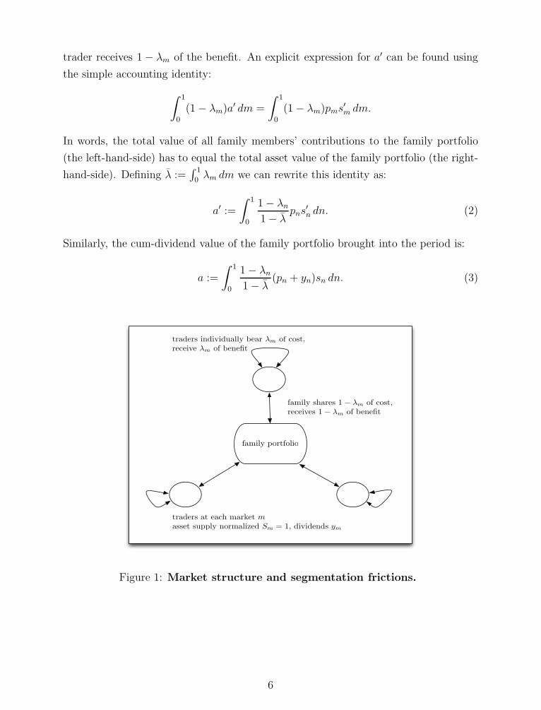
Segmentation frictions. We interpret the representative family as a partially inte-

grated financial system. Each trader in market m works at a specialized trading desk

that deals in the asset specific to that market (Figure 1 illustrates). Traders in market

m are assumed to bear an exogenous fraction 0 ≤ λm ≤ 1 of the cost of trading in that

market and in return receive λm of the benefit. The remaining 1 − λm of the cost and

return of trading in that market is shared between family members.

More precisely, given segmentation parameter λm, the period budget constraint

facing a representative trader in market m is:

cm + λmpms′m + (1 − λm)a′ ≤ λm(pm + ym)sm + (1 − λm)a, (1)

where pm is the ex-dividend price of a share in the asset in market m, and sm, s′m

represent share holdings in that asset. The two terms a and a′ are the cum-dividend

value of the family portfolio brought into the period and the ex-dividend value of the

family portfolio acquired this period, respectively.

As can be seen from the budget constraint, a trader in market m holds directly a

number λms′m of shares of asset m. The cost of acquiring all the remaining shares in

the economy,∫

1

0

(1 − λm)pms′m dm,

is divided among all the family members. More specifically, the term (1− λm)a′ on the

left-hand side of the budget constraint (1) means that the trader in market m is asked

to contributes 1 − λm of the cost of acquiring all the remaining shares. Symmetrically,

the term (1 − λm)a on the right-hand side of the budget constraint means that the

5

trader receives 1 − λm of the benefit. An explicit expression for a′ can be found using

the simple accounting identity:

∫

1

0

(1 − λm)a′ dm =

∫

1

0

(1 − λm)pms′m dm.

In words, the total value of all family members’ contributions to the family portfolio

(the left-hand-side) has to equal the total asset value of the family portfolio (the right-

hand-side). Defining λ :=∫

1

0λm dm we can rewrite this identity as:

a′ :=

∫

1

0

1 − λn

1 − λpns

′n dn. (2)

Similarly, the cum-dividend value of the family portfolio brought into the period is:

a :=

∫

1

0

1 − λn

1 − λ(pn + yn)sn dn. (3)

family portfolio

traders individually bear λm of cost,

receive λm of benefit

family shares 1 − λm of cost,

receives 1 − λm of benefit

traders at each market m

asset supply normalized Sm = 1, dividends ym

Figure 1: Market structure and segmentation frictions.

6

2.2 Equilibrium asset pricing

The Bellman equation for the family’s value function is

v(s, y) = maxc,s′

{∫

1

0

u(cm) dm+ βE[v(s′, y′)|y]}

. (4)

The maximization is over choices of consumption allocations c : [0, 1] → R+ and asset

holdings s′ : [0, 1] → R, specifying cm and s′m for each m ∈ [0, 1]. The maximization

is taken subject to the collection of budget constraints (1), one for each m, and the

accounting identities for the family portfolio in (2) and (3). The expectation on the

right-hand-side of the Bellman equation is formed using the conditional distribution for

y′ given the current aggregate endowment y.

An equilibrium of this economy is a collection of functions {c, p, s′} such that (i)

taking p : [0, 1] → R+ as given, c : [0, 1] → R

+ and s′ : [0, 1] → R solve the family’s

optimization problem (4), and (ii) asset markets clear: s′m = 1 for all m.

Equilibrium allocation. Before solving for asset prices, we provide the equilibrium

allocation of consumption across market. Substituting the accounting identities (2) and

(3) into the budget constraint (1) and imposing the equilibrium condition s′m = 1, we

obtain:

cm = λmym + (1 − λm)

∫

1

0

1 − λn

1 − λyn dn.

And since the realized idiosyncratic yn are independent of λn, an application of the Law

of Large Numbers gives:

cm = λmym + (1 − λm)y. (5)

This formula is intuitive: equilibrium consumption in market m is a weighted average

of the idiosyncratic and aggregate endowments with weights reflecting the degree of

market segmentation. The λm represent the extent to which traders are not fully

diversified and hence the segmentation parameters determine the degree of risk sharing

in the economy. If λm = 0, traders are fully diversified and will have consumption equal

to the aggregate endowment cm = y (i.e., full consumption insurance). But if λm = 1,

traders are not at all diversified and will simply consume the dividends realized in their

specific market cm = ym (i.e., autarky).

Asset prices. To obtain asset prices, we use the first-order condition of the family’s

optimization problem. Let µm ≥ 0 denote the Lagrange multiplier on the family’s

budget constraint for market m. We show in Appendix A that the family’s Lagrangian

7

can be written:

L =

∫

1

0

[

u(cm) + qm(pm + ym)sm − qmpms′m − µmcm

]

dm+ βE[v(s′, y′)|y],

where

qm := λmµm + (1 − λm)

∫

1

0

1 − λn

1 − λµn dn, (6)

is a weighted average of the Lagrange multipliers in market m and the multipliers for

other markets with weights reflecting the various degrees of market segmentation. More

specifically, qm is the marginal value to the family of earning one (real) dollar in market

m. The first term in (6) arises because a fraction λm goes to the local trader, with

marginal utility µm. The second term arises because the remaining fraction is shared

among other family members, with marginal utility µn, according to their relative

contributions (1 − λn)/(1 − λ) to the family portfolio. We will refer to qm as the state

price of earning one real dollar in market m.

Just as equilibrium consumption in market m is a weighted average of the idiosyn-

cratic or “local” endowment and aggregate endowment with weights λm and 1−λm, so

too the state price for market m is a weighted average of the idiosyncratic multiplier

and an aggregate multiplier with the same weights. To highlight this, define

q :=

∫

1

0

1 − λn

1 − λµndn (7)

so that we can write qm = λmµm + (1 − λm)q. If any particular market m has λm = 0

then the state price in that market is equal to the aggregate state price qm = q and

is independent of the local endowment realization. If the segmentation parameter is

common across markets, λm = λ all m, then q is the cross-sectional average marginal

utility and q =∫

1

0qmdm. More generally, q is not a simple average over µm since

different markets have different relative contribution (1 − λm)/(1 − λ) to the family

portfolio.

The first order conditions of the family’s problem are straightforward. For each cm

we have:

u′(cm) = µm. (8)

And for each s′m we have:

qmpm = βE

[

∂v

∂s′m(s′, y′)

∣

∣

∣

∣

y

]

. (9)

8

The Envelope Theorem then gives:

∂v

∂sm(s, y) = qm(pm + ym). (10)

Combining equations (9) and (10) gives the Euler equation characterizing asset prices

in each market:

pm = E

[

βq′mqm

(p′m + y′m)

∣

∣

∣

∣

y

]

. (11)

The Euler equation for asset prices takes a standard form, familiar from Lucas (1978),

with the crucial distinction that the stochastic discount factor (SDF), βq′m/qm, is market

specific.

Note that, combining the formulas for equilibrium consumption, (5), market-specific

state prices, (6), and the pricing equation (11), we obtain a mapping from the primitives

of the economy (the λm, ym etc) into equilibrium asset prices. In particular, one easily

verify that the Lucas (1978) asset prices are obtained in the further special case λm = 0

all m, so that cm = y all m and µm = u′(y) all m and q =∫

1

0u′(y) dn = u′(y).

Shadow prices of risk-free bonds. To simplify the presentation of the model, we

have not explicitly introduced risk-free assets. But we can still compute “shadow” bond

prices. Let πk denote the price of a zero-coupon bond pays one unit of the consumption

good for sure in k ≥ 1 period’s time and that is held in the family portfolio. As shown

in Appendix A these bonds would have price:

πk = E

[

βq′

qπ′

k+1

∣

∣

∣

∣

y

]

, (12)

with π0 := 1. Bonds are priced using the aggregate state price q. In particular,

the one-period shadow gross risk-free rate is given by 1/π1 = 1/E [βq′/q]. Although

the one-period SDF for bonds βq′/q does not depend on any particular idiosyncratic

endowment realization, it does depend on the distribution of idiosyncratic endowments

and in general is not simply the Lucas (1978)-Breeden (1979) SDF.

3 Calibration

To evaluate the significance of these segmentation frictions, we calibrate the model.

9

3.1 Parameterization of the model

Preferences and endowments. Let period utility u(c) be CRRA with coefficient

γ > 0 so that u′(c) = c−γ . The log aggregate endowment is a random walk with drift

and IID normal innovations:

log gt+1 := log(yt+1/yt) = log g + ǫg,t+1, ǫg,t+1 ∼ IID and N(0, σ2

ǫg), g > 0. (13)

Log market-specific endowments are the log aggregate endowment plus an idiosyncratic

term:

log ym,t := log yt + log ym,t, (14)

so that market-specific endowments inherits the trend in the aggregate endowment. The

log idiosyncratic endowment log ym,t is conditionally IID normal in the cross-section:

log ym,t ∼ IID and N(−σ2

t /2, σ2

t ), (15)

where the mean of −σ2t /2 is chosen to normalize Et[ym,t] = 1 and Et[ym,t] = yt.

Idiosyncratic endowment volatility. Volatility of the idiosyncratic endowment in

a given market is time-varying and given by an AR(1) process in logs:

log σt+1 = (1 − φ) log σ + φ log σt + ǫv,t+1, ǫv,t+1 ∼ IID and N(0, σ2

ǫv), σ > 0. (16)

In a frictionless model (λm = 0 all m), all idiosyncratic risk would be diversified away

so that asset prices would be independent of σt. With segmentation frictions (λm > 0),

by contrast, both the level and dynamics of σt will affect asset prices.

Solving the quantitative model. Since ym,t = ym,t/yt we can use equation (5) to

write equilibrium consumption in market m as the product of the aggregate endow-

ment yt and an idiosyncratic component that depends only on the local idiosyncratic

endowment realization ym,t and the amount of segmentation:

cm,t = [1 + λm(ym,t − 1)]yt. (17)

Similarly, we can then use this expression for consumption and the fact that utility is

CRRA to write the local state price as:

qm,t = θm,ty−γt , (18)

10

where:

θm,t := λm[1 + λm(ym,t − 1)]−γ + (1 − λm)

∫

1

0

1 − λn

1 − λ[1 + λn(yn,t − 1)]−γ dn. (19)

The SDF for market m is then:

Mm,t+1 := βg−γt+1

θm,t+1

θm,t

. (20)

This is the usual Lucas (1978)-Breeden (1979) aggregate SDF Mt+1 := βg−γt+1 with a

market-specific multiplicative “twisting” factor Mm,t+1 := θm,t+1/θm,t that adjusts the

SDF to account for idiosyncratic endowment risk.

To solve the model in stationary variables, let pm,t := pm,t/yt denote the price-to-

aggregate-dividend ratio for market m. Dividing both sides of equation (11) by yt > 0

and using gt+1 := yt+1/yt this ratio solves the Euler equation:

pm,t = Et

[

βg1−γt+1

θm,t+1

θm,t(pm,t+1 + ym,t+1)

]

, (21)

which is the standard CRRA-formula except for the multiplicative adjustment θm,t+1/θm,t.

This is a linear integral equation to be solved for the unknown function mapping the

state into the price/dividend ratio. In general this integral equation cannot be solved

in closed form, but numerical solutions can be obtained in a straightforward manner

along the lines of Tauchen and Hussey (1991). We discuss these methods in greater

detail in Appendix B below.

3.2 Calibration strategy and results

We calibrate the model using monthly postwar data (1959:1-2007:12, unless otherwise

noted). Following a long tradition in the consumption-based asset pricing literature, we

interpret the aggregate endowment as per capita real personal consumption expenditure

on nondurables and services. We set log g = (1.02)1/12 to match an annual 2% growth

rate and σǫg = 0.01/√

12 to match an annual 1% standard deviation over the postwar

sample. We set β = (0.99)1/12 to reflect an annual pure rate of time preference of 1%

and we set the coefficient of relative risk aversion to γ = 4.

For our benchmark calibration we assume that all markets in the economy share the

same segmentation parameter, λ. Given the values for preference parameters β, γ and

the aggregate endowment growth process g, σǫg above, we still need to assign values to

this single λ and the three parameters of the cross-sectional dispersion process σ, φ, σǫv.

11

Calibrating the idiosyncratic volatility process. The crucial consequence of

market segmentation is that local traders are forced to bear some idiosyncratic risk.

Thus, to explain the impact of market segmentation on risk premia, it is important

that our model generates realistic levels of idiosyncratic risk. This leads us to choose

the parameters of the stochastic process for idiosyncratic endowment volatility in order

to match key features of the volatility of a typical stock return. To see why there is a

natural mapping between the two volatilities, write the gross returns on stock m as:

Rm,t = gtym,t + pm,t

pm,t−1

. (22)

Thus, the volatility of ym,t directly affects stock returns through the dividend term of

the numerator. It also indirectly affects stock returns through the asset price, pm,t.

We obtain key statistics about stock return volatility from Goyal and Santa-Clara

(2003). Their measure of monthly stock volatility is obtained by adding up the ob-

tained by adding up the cross-sectional stock return dispersion over each day of the

previous month. In Figure 2 we show the monthly time series (1963:1-2001:12) of

their measure of the cross-sectional standard deviation of stock returns, as updated by

Bali, Cakici, Yan, and Zhang (2005).

1960 1970 1980 1990 20005

10

15

20

25

30

35

40

1960 1970 1980 1990 2000

−30

−20

−10

0

10

20

30

40

50

60

70

stock returns dispersion

HP trend

deviation from HP trend

per

cent

stan

dar

ddev

iati

on

per

cent

dev

iati

onfr

omtr

end

monthmonth

Figure 2: Cross-sectional standard deviation of stock returns (1963:1-2001:12) fromGoyal and Santa-Clara (2003), as updated by Bali et al. (2005).

12

We choose the idiosyncratic endowment volatility process so that, when we calculate

the same stock return volatility measure in our model, we replicate key features of this

data. We replicate three features of the data: the unconditional average return volatility

of 16.4%, the unconditional standard deviation of return volatility 4.2% monthly, and

AR(1) coefficient of return volatility 0.84 monthly. We replicate these three features

by simultaneously choosing the three parameters governing the stochastic process for

endowment volatility: the unconditional average σ, the innovation standard deviation

σǫv, and the AR(1) coefficient φ.

Calibrating the segmentation parameter: basics. The segmentation parameter

λ governs the extent to which local traders can diversify away the return volatility of

their local asset. Thus, λ determines the extent to which the idiosyncratic volatility

factor, σt, has an impact on asset prices and creates systematic variation in asset returns.

This leads us to identify λ using a measure of systematic volatility, the return volatility

of a well diversified portfolio.

To understand precisely how the identification works, recall first what would hap-

pen in the absence of market segmentation, λ = 0. Then, we would be back in the

Lucas (1978)-Mehra and Prescott (1985) model with IID lognormal aggregate endow-

ment growth. As is well known (see, e.g., LeRoy, 2006), this model can’t generate

realistic amounts of systematic volatility. Specifically, with λ = 0 the return from a di-

versified market portfolio is gt(1+p)/p where p = βE[g1−γ]/(1−βE[g1−γ]) is the constant

price/dividend ratio for the aggregate market. With our standard parameterization of

the preference parameters and aggregate endowment growth, (1+ p)/p ≈ 1.0058 so that

the monthly standard deviation of the diversified market portfolio return is approxi-

mately the same as the monthly standard deviation of aggregate endowment growth,

about 0.29% monthly as opposed to about 4.28% monthly in the data.

In contrast with the λ = 0 case, when λ > 0 idiosyncratic endowment volatility

creates systematic volatility. Indeed, because of persistence, a high idiosyncratic en-

dowment volatility this month predicts a high idiosyncratic endowment volatility next

month. Thus in every market m local traders expect to bear more idiosyncratic risk,

and because of risk aversion the price dividend ratio pm,t has to go down everywhere.

Because this effect impacts all stocks at the same time, it endogenously creates system-

atic return volatility. Clearly, the effect is larger if markets are more segmented and

traders are forced to bear more idiosyncratic risk: thus, a larger λ will result in a larger

increase in systematic volatility.

13

Calibrating the segmentation parameter: specifics. We consider two calibra-

tion schemes. In our benchmark calibration, we identify λ by matching the return

volatility of a well-diversified portfolio, specifically the 4.3% monthly standard devia-

tion of the real value-weighted return of NYSE stocks from CRSP. In a second, more

conservative, calibration, we identify λ by matching only the fraction of the aggregate

volatility of stock returns that is systematically explained by idiosyncratic stock return

volatility (i.e., the Goyal and Santa-Clara, 2003, factor). Goyal and Santa-Clara find

that the correlation between the systematic volatility of value-weighted stock returns

and idiosyncratic stock return volatility is about 0.4 at a monthly frequency. There-

fore, if idiosyncratic stock return volatility was the only source of systematic return

volatility, systematic volatility should only be about 0.4× 4.3% = 1.72% monthly. Im-

plicitly, this procedure leaves other factors outside the model to explain the remaining

0.6 × 4.3% = 2.58% monthly of the systematic volatility observed in the CRSP data.

Since our second calibration selects λ to reproduce this counterfactually lower level of

systematic volatility, it naturally leads to a lower calibrated value for λ.

Calibration results. The calibrated parameters from these two schemes are listed

in Table 1. In our benchmark calibration, the level of λ is 0.21. That is, 21% of

idiosyncratic endowment risk is non-tradeable. In terms of portfolio weights, we also

find that λ = 0.21 implies that, in a typical market m, a trader invests approximately

21% of his wealth in the local asset, and the rest in the family portfolio.3

Our more conservative calibration necessarily selects a lower level of λ, but in prac-

tice the difference is small: the conservative calibration of λ is 0.19. Thus there is a

relatively small difference in λ despite the fact that the conservative calibration targets

systematic stock return volatility that is only 40% of actual systematic stock volatility.

The differences between the calibrations are more significant for the cross-sectional en-

dowment volatility process. In the benchmark, the volatility process is more persistent

and has bigger innovations but fluctuates around a lower unconditional mean.

Table 2 shows that with these parameters, the benchmark model matches the target

moments closely but not exactly. Notice that in the benchmark calibration the per-

sistence of the cross-sectional endowment distribution φ is close to one.4 That is, to

match the persistence in the data, the calibration procedure tries to select a very high

φ. As explained above, persistence is necessary for idiosyncratic volatility to matter

3The derivation of portfolio weights for the family is given in Appendix A below.4The discrete-state approximation of the process for σt (equation 16) used to solve the model is

stationary by construction, even when φ = 1 exactly. See Appendix B for more details on our solutionmethod.

14

for systematic stock return volatility. Thus, the value of φ is high largely because the

model is matching a high level of systematic volatility. This intuition is confirmed by

the conservative calibration: when we target a lower level of systematic volatility, the

calibration procedure gives a lower value, φ = 0.89, and the model remains able to hit

the persistence of the cross-sectional standard deviation of returns exactly.

4 Quantitative examples

Aggregate statistics. In comparing our model to data, we adopt the perspective of

an econometrician who observes a collection of asset returns but who ignores the pos-

sibility of market segmentation. In particular, to make our results comparable to those

typically reported in the empirical asset pricing literature, we focus on the properties

of the aggregate market portfolio. We define the gross market return RM := (p′ + y′)/p

where p :=∫

1

0pm dm is the ex-dividend value of the market portfolio and y is the

aggregate endowment. We define the gross (shadow) risk free rate for market m by

Rf,m := E[βq′m/qm]−1 and the average risk free rate by Rf :=∫

1

0Rf,m dm. We then

calculate the unconditional equity risk premium E[RM −Rf ] by and similarly for other

statistics. We call p/y the price dividend ratio of the market.

4.1 Results

Equity premium. With these definitions in mind, Table 3 shows our model’s impli-

cations for aggregate returns and price/dividend ratios. We report annualized monthly

statistics from the model and compare these to annualized monthly returns and to

annual price/dividend ratios (we use annual data for price/dividends because of the

pronounced seasonality in dividends at the monthly frequency). The benchmark model

produces an annual equity risk premium of 3.69% annual as opposed to about 5.27%

annual in the postwar NYSE CRSP data. Clearly this is a much larger equity premium

than is produced by a standard Lucas (1978)-Mehra and Prescott (1985) model. For

comparison, that model with risk aversion γ = 4 and IID consumption growth with

annual standard deviation of 1% produces an annual equity premium of about 0.04%.

The segmented markets model with λ = 0.21 is able to generate an equity premium

some two orders of magnitude larger.

Why is there a large equity premium? Relative to standard consumption-based

asset pricing models with time-separable expected utility preferences, our model delivers

a large equity premium. We use our parameter λ to generate realistically high levels

15

of systematic market volatility. Is matching systematic return volatility what helps

us generate a large equity premium? No. Recall from the GMM estimates of risk

aversion in Hansen and Singleton (1982) (and others) that the standard consumption-

based model fails to match the equity premium in the data even when — by construction

— it matches the systematic return volatility in the data. But of course model risk

premia are generated by covariances so no matter how much systematic return volatility

you feed into a model, the equity risk premia will be zero if the model’s SDF is not

correlated with that systematic return volatility (see Cochrane and Hansen, 1992, for

a forceful argument).

What, then, is the equity premium from the point of view of aggregate consumption?

One can show that, in our model, if one computes the unconditional average equity

premium using the model generated market return and the Lucas (1978)-Breeden (1979)

SDF βg−γt+1 instead of the true model SDF, then the equity premium is on the order of

0.04% (4 basis points) annual rather than the 3.69% annual in the benchmark model.

While aggregate consumption does not command a big risk premium, the volatility

factor does. To see this, consider the premium implied by the SDF βqt+1/qt where q is

aggregate state price that determines the (shadow) price of risk free bonds. In general

this is given by equation (7) but with a single common λ it reduces to q =∫

1

0µm dm =

∫

1

0c−γm dm, the cross-section average marginal utility. In our benchmark model, this

SDF implies an equity premium of 2.17% annual. This comes from the convexity of

the marginal utility function: a high realization of σt makes equilibrium consumption

highly dispersed across markets so that average marginal utilities are high. At the same

time, a high σt depresses asset prices in every market, so that the return on the market

portfolio is high.

Level of the risk-free rate. Although the benchmark model delivers reasonable im-

plications for the level of the equity premium, it is not so successful on other dimensions

of the data. The level of the risk free rate is very high as compared to the data. In the

model the risk free rate is about 8 or 9% annual, while in the data it is more like 2%. As

emphasized by Weil (1989), this is a common problem for models with expected-utility

preferences. In short, attempts to address the equity premium puzzle by increasing risk

aversion also tend to raise the risk free rate so that even if it’s possible to match the

equity premium, the model may well do so at absolute levels of returns that are too

high. This effect comes from the relationship between real interest rates and growth in

a deterministic setting with expected utility, high risk aversion means low intertemporal

elasticity of substitution so that it takes high real interest rates to compensate for high

16

aggregate growth. With risk, there is an offsetting precautionary savings effect that

could, in principle, pull the risk free rate back down to more realistic levels. But in our

calibration this precautionary savings effect is quantitatively small: raising λ from zero

(the Mehra and Prescott case) to λ = 0.21 (our benchmark) lowers the risk free rate

by about 1% annual.

Volatility of the risk-free rate. In the data, the risk free rate is smooth and the

volatility of the equity premium reflects the volatility of equity returns. In the bench-

mark model, the risk free rate is too volatile, about 11% annual as opposed to 1%

annual in the data.

Price/dividend ratio. The benchmark model produces an annual price/dividend

ratio of about 12 as opposed to an unconditional average of more like 31 in the NYSE

CRSP data. Given the large, persistent, swings in the price/dividend ratio in the data,

what constitutes success on this dimension is not entirely clear. The model generates

if anything slightly too much unconditional volatility in the log price/dividend ratio,

some 43% annual as opposed to 39% in the data. This is another reflection of the fact

that the model by construction matches the aggregate volatility of the market. While

the unconditional volatility of the price/dividend ratio is similar in the model and in the

data, the temporal composition of this volatility is somewhat different. In particular,

the persistence of the log price/dividend ratio is about 0.50 annual in the benchmark

model, lower than the 0.88 in the data. That is, the unconditional volatility of the

price/dividend ratio in the data comes from large, low-frequency movements whereas

the unconditional volatility in the model comes from higher-frequency movements.

4.2 Discussion

Constant endowment volatility. Our benchmark model has two departures from

a standard consumption-based asset pricing model: segmentation and a time-varying

endowment volatility. To show that both these departures are essential for our results,

we solved our model with constant endowment volatility, i.e., σt = σ all t. For this

exercise, we fix the volatility at the same level as the unconditional average from the

benchmark model σ = 1.71 and keep the level of segmentation at the benchmark

λ = 0.21. In Table 2 we show that this “constant σ” version of the model produces

essentially the same amount of unconditional cross-sectional stock return volatility as

in the data (suggesting that this moment is principally determined by σ alone) but

17

produces only as much systematic stock volatility as would a benchmark Lucas (1978)-

Mehra and Prescott (1985) model, about 0.29% monthly as opposed to 4.28% in the

data. Thus λ > 0 is necessary but not sufficient for our model to create systematic

stock volatility from idiosyncratic endowment volatility. In Table 3 we see that despite

producing negligible systematic stock volatility, the model with constant σ is capable

of generating a modest equity premium, some 1.29% annual. The benchmark model

with time variation in endowment volatility generates another 2.4% on top of this for

a total of 3.69% annual.

Countercyclical endowment volatility. Many measures of cross-sectional idiosyn-

cratic risk increase in recessions.5 This counter-cyclicality is also a feature of the

cross-sectional standard deviation of returns data from Goyal and Santa-Clara (2003).

However, the stochastic process we use for the cross-sectional volatility evolves inde-

pendently of aggregate growth. To see if our results are sensitive to this, we modify the

stochastic process in (16) to:

log σt+1 = (1 − φ) log σ + φ log σt − η(log gt − log g) + ǫv,t+1. (23)

with ǫv,t+1 IID normal, as before. If η > 0, then aggregate growth below trend in period

t increases the likelihood that volatility is above trend in period t+ 1 so that volatility

is counter-cyclical. We identify the new parameter η by requiring that, in a regression

of the cross-section standard deviation of stock returns on lagged aggregate growth, the

regression coefficient is −0.50 as it is in the data. The calibrated parameters for this

“feedback” version of the model are also shown in Table 1. The calibrated η elasticity

is 1.88 so aggregate growth 1% below trend tends to increase endowment volatility by

nearly 2%. The other calibrated parameters are indistinguishable from the benchmark

parameters. Moreover, the model’s implications for asset prices as shown in Table 3

are also very close to the results for the benchmark model. This suggests that while

the model can be reconciled with the countercyclical behavior of cross-sectional stock

volatility, this feature is not necessary for our main results.

Relationship to incomplete markets models. There is a large literature in macroe-

conomics that analyzes the asset pricing implications of market incompleteness when

households receive uninsurable idiosyncratic income shocks.6 One might have the im-

pression that all our model does is shift the focus of incomplete markets models from

5See for example Campbell, Lettau, Malkiel, and Xu (2001) and Storesletten et al. (2004).6See for example Telmer (1993) and Heaton and Lucas (1996).

18

the idiosyncratic labor income risk facing households to the idiosyncratic income risk

faced by the financial sector. We argue that, while our segmented markets model in-

deed results in uninsurable shocks, it is conceptually different from standard incomplete

markets models.

To see why, note that in standard incomplete markets models the intertemporal

marginal rate of substitution (IMRS) of every household i prices the excess return of

the market portfolio:

E [MiRe] = 0. (24)

As forcefully emphasized by Mankiw (1986), Constantinides and Duffie (1996) and

Kruger and Lustig (2008), with CRRA utility when idiosyncratic consumption growth

is statistically independent from aggregate consumption growth, idiosyncratic risk has

no impact on the equity premium. Indeed, in that case the IMRS can be factored

into MiM , where M = βg−γ is the standard Lucas (1978)-Breeden (1979) stochastic

discount factor, and Mi is an idiosyncratic component that is independent from M .

Expanding the expectation in (24) we have:

E[MiMRe] = E[Mi]E[MRe] + Cov[Mi,MRe] = 0.

From independence Cov[Mi,MRe] = 0. Using this and dividing both sides by E[Mi] > 0

we obtain:

E [MRe] = 0. (25)

As shown by Kocherlakota (1996), this asset pricing equation cannot rationalize the

observed equity premium.

In our benchmark model, we maintain the assumption that the idiosyncratic compo-

nent of dividends, ym, is statistically independent from aggregate consumption growth.

Yet, we obtain a much larger equity premium than Mehra and Prescott. The reason for

this is that in our asset pricing model the local stochastic discount factor does not have

to price the excess return on the aggregate market portfolio, as in equation (24), but

instead price the excess return on the local asset market. The local discount factor is

correlated with the local excess return (through the local endowment realization) and

this makes it impossible to strip-out the influence of market-specific factor.

Specifically, instead of equation (24) we have a pricing equation of the form:

E [MmRem] = 0, (26)

where Mm is the local stochastic discount factor and Rem is the local excess return. From

19

equation (20) we can factor the local discount factor into MmM where M is again the

Lucas (1978)-Breeden (1979) discount factor and Mm is a market-specific factor. Now

proceeding as above and expanding the expectation in (26) we have:

E[MmMRem] = E[Mm]E[MRe

m] + Cov[Mm,MRem] = 0.

But Mm and Rem depend on the same local risk factor so Cov[Mm,MRe

m] 6= 0 and we

cannot factor out E[Mm]. Because this makes it impossible to aggregate the collection

of equations (26) into (24), in our model the standard incomplete markets logic does

not apply.

5 Cross-sectional volatilities

In our first set of quantitative examples we used a common amount of segmentation,

λ, for all asset markets. This implies that conditional on the aggregate state of the

economy, each market m is characterized by a common amount of volatility (essentially

determined by the economy-wide σt and λ) so that there is no cross-sectional variation

in volatility. We now pursue the implications of the general model with market-specific

λm and hence a non-degenerate cross-section of volatility.

Specifically, we allow for a finite number of market types. In a slight abuse of

notation we continue to index these market types by m. We assume that each market

contains the same number of assets, but that there is a total measure ωm of traders

in market m, with a supply per trader normalized to 1. With this notation, then, the

aggregate endowment is y =∑

m ymωm, etc.

Calibration of market-specific λm: strategy. In the case of a single common λ

above, the value of λ was identified by matching a measure of systematic volatility,

the return volatility of a well-diversified portfolio of stocks. We now need to identify a

vector of segmentation parameters and we do this using a closely-related strategy. In

particular, we identify market types with quintile portfolios of stocks sorted on measures

of idiosyncratic volatility from Ang, Hodrick, Xing, and Zhang (2006). They compute

value-weighted quintile portfolios by sorting stocks based on idiosyncratic volatility

relative to the Fama and French (1993) three-factor pricing model in postwar CRSP

data. To give a sense of this data, Ang, Hodrick, Xing, and Zhang report an average

standard deviation of (diversified) portfolio returns for the first quintile of stocks of

about 3.83% monthly (as opposed to about 4.28% for the market as a whole). By

20

construction this portfolio is 20% of a simple count of stocks but it constitutes about

53.5% of the market by value. At the other end of the volatility spectrum, the average

monthly standard deviation of a well-diversified portfolio of the fifth quintile of stocks

is about 8.16% and these constitute only about 1.9% of the market by value.

We choose the value of λm for m = 1, ..., 5 to match the unconditional average id-

iosyncratic volatility of the m’th quintile portfolio in Ang, Hodrick, Xing, and Zhang.

Since our model has no counterpart of Fama and French’s size and book/market fac-

tors, we construct a measure of idiosyncratic volatility relative to a single-factor CAPM

model. For each market m in the model we obtain the residuals from a CAPM re-

gression of individual market returns on the aggregate market return and use these

residuals to compute idiosyncratic volatility for each market. Similarly, we choose

values of ωm so that the unconditional average portfolio weight7 of the family in as-

sets of market m matches the average market share for the m’th quintile portfolio

from Ang, Hodrick, Xing, and Zhang (2006). Our calibration procedure chooses these

parameters simultaneously with the parameters σ, φ, σǫv of the stochastic process for

cross-sectional endowment volatility. We keep the values of the preference parameters

β, γ and the aggregate growth parameters g, σǫg at their benchmark values.

Calibration of market-specific λm: results. The calibrated parameters from this

procedure are listed in Table 4. We find that the m = 1 market, with the lowest

idiosyncratic volatility, has a segmentation parameter λ1 = 0.00 (to two decimal places).

These assets are essentially frictionless. This m = 1 market consists of 20% of assets by

number, by construction, but it accounts for 50% of total market by value. By contrast,

the m = 5 market has segmentation parameter λ5 = 0.33 but accounts for only 2% of

total market value. Across markets the segmentation parameters λm are monotonically

increasing inm while the weights ωm are monotonically decreasing inm. Averaging over

the five markets λ =∑

m λmωm = 0.11. Thus this economy, which matches the same

aggregate moments as the benchmark model, hits its targets with an average amount of

segmentation λ = 0.11 roughly half that of the single parameter benchmark λ = 0.21.

This suggests that there may be a significant bias when aggregating a collection of

heterogeneously segmented markets into a “representative” segmented market.

Relative to the benchmark, the model’s endowment volatility process now has a

lower unconditional average, more time-series variation, and slightly less persistence.

Table 5 shows that with these parameters the model matches the target moments closely

but not exactly. In particular, while the average idiosyncratic volatility across the m

7The derivation of portfolio weights for the family is given in Appendix A below.

21

markets is about 4.6% monthly as opposed to 4.7% in the data, this is achieved with

slight discrepancies at the level of each market, e.g., the 1st market has volatility of

3.8% against 4.2% in the data.

Market-specific asset pricing implications. In Panel A of Table 6 we show the

risk premia and CAPM parameters for each market type in the model and their empir-

ical counterparts. In the data, the equity premia for the low volatility m = 1 market is

0.53% monthly (roughly 6.5% annual) whereas in the model it is 0.18% monthly. This

market accounts for half of total market value and has an alpha of about 0.14 in the

data and 0.11 in the model. As we go to markets with higher volatility, the model

predicts that risk premia monotonically increase, reaching 0.85% monthly (or 10.6%

annual) for the m = 5 market. However, the data predicts a hump-shaped pattern for

the cross-section of equity premia, with the premia reaching a maximum at about 0.69%

monthly for the m = 3 market before falling to −0.53% for the 5th and most volatile

market. Thus the model fails to account even qualitatively for the equity premia of the

highest idiosyncratic volatility markets.

Aggregate asset pricing implications. In Panel B of Table 6 we show the aggre-

gate asset pricing implications of the model with market-specific λm. The aggregate

equity premium is essentially the same as in the benchmark single λ model, 3.6% an-

nual, despite the fact that the average segmentation here is only λ = 0.11, half the

single λ benchmark. For comparison, the table shows the asset pricing implications for

an otherwise identical single λ economy with λ = λ = 0.11. The aggregation of the

micro segmentation frictions across the different markets adds some 1.6% annual to the

equity premium, taking it from 2% to 3.6%. This model generates about twice as much

time-series volatility in the equity premium as the benchmark, some 1.8% as opposed

to 0.9% annual, but still an order of magnitude lower than the 14% annual in postwar

NYSE CRSP data. Compared to the benchmark model, the risk free rate has about

the same level and if anything is even more volatile.

6 Conclusion

We propose a tractable consumption-based model in order to explain and quantify

the macro impact of financial market frictions. We envision an economy comprised of

many micro financial markets that are partially segmented from one another. Because

of segmentation, traders in each micro market have to bear some local idiosyncratic risk.

22

Assets in every markets are priced by a convex combination of the local trader marginal

utility (who has to bear some of the idiosyncratic risk), and of the average marginal

utility in the rest of the economy (who can diversify the remaining idiosyncratic risk

in a large portfolio). We calibrate the model when all markets share the same level

of segmentation and show that it can generate a sizeable equity premium. We also

allow segmentation to differ across markets and show that aggregation matters: we can

obtain essentially the same aggregate asset pricing implication with a much smaller

average level of segmentation.

23

Tables

Panel A: Preferences and aggregate endowment growth.

Parameter Monthly value Notes

β 0.9992 annual discount rate 1%γ 4 coefficient relative risk aversiong 1.0017 annual aggregate growth 2%σǫg 0.0029 annual std dev aggregate growth 1%

Panel B: Segmentation and idiosyncratic endowment volatility.

ModelParameter Benchmark Conservative Feedback Data moment

λ 0.21 0.19 0.21 std dev diversified market portfolio return 4.28σ 1.71 2.30 1.71 average cross-section std dev returns 16.40σǫv 0.10 0.04 0.10 time-series std dev cross-section std dev returns 4.17φ 0.99 0.89 0.99 AR(1) cross-section std dev returns 0.84η 1.88 regression cross-section std dev returns on lagged growth −0.50

Table 1: Parameter choices.

24

ModelMoment Data Benchmark Conservative Constant Feedback

std dev diversified market portfolio return 4.28 4.21 1.81 0.29 4.21average cross-section std dev returns 16.40 16.37 16.40 14.46 16.36time-series std dev cross-section std dev returns 4.17 4.18 4.17 0.00 4.18AR(1) cross-section std dev returns 0.84 0.78 0.84 0.78regression cross-section std dev returns on lagged growth −0.50 −0.50

Table 2: Fit of calibrated models.

ModelMoment Data Benchmark Conservative Constant Feedback

equity premium E[RM − Rf ] 5.27 3.69 1.87 1.29 3.68market return E[RM ] 7.04 12.29 11.08 10.54 12.33risk free rate E[Rf ] 1.78 8.59 9.21 9.25 8.64

Std[RM − Rf ] 14.25 0.88 0.28 0.00 0.89Std[RM ] 14.44 14.60 6.27 1.01 14.60Std[Rf ] 1.06 11.29 5.92 0.00 11.71

sharpe ratio E[RM − Rf ]/Std[RM − Rf ] 0.37 4.20 6.80 4.12

price/dividend ratio E[p/y] 30.81 12.58 12.18 12.40 12.59Std[log(p/y)] 38.63 43.21 12.29 0.00 43.15Auto[log(p/y)] 0.88 0.50 0.20 0.50

Table 3: Aggregate asset pricing implications of single λ model.

25

Panel A: Segmentation parameters.

Model Data momentMarket m λm ωm Portfolio std dev Market share

1 0.00 0.50 3.8 0.542 0.17 0.28 4.7 0.273 0.25 0.13 5.9 0.124 0.30 0.06 7.1 0.055 0.33 0.02 8.2 0.02

average 0.11 4.6

Panel B: Idiosyncratic endowment volatility.

Parameter Data moment

σ 1.12 average cross-section std dev returns 16.40σǫv 0.18 time-series std dev cross-section std dev returns 4.17φ 0.97 AR(1) cross-section std dev returns 0.84

Table 4: Market-specific segmentation.

26

Panel A: Segmentation parameters.

Data moment Model momentMarket m Portfolio std dev Market share Portfolio std dev Market share

1 3.8 0.54 4.2 0.542 4.7 0.27 4.6 0.273 5.9 0.12 5.7 0.124 7.1 0.05 7.0 0.055 8.2 0.02 8.1 0.02

average 4.6 4.7

Panel B: Idiosyncratic endowment volatility.

Moment Data Model

average cross-section std dev returns 16.40 16.50time-series std dev cross-section std dev returns 4.17 4.20AR(1) cross-section std dev returns 0.84 0.85

Table 5: Fit of market-specific segmentation model.

27

Panel A: Market-specific asset pricing implications.

Risk premia CAPM alpha CAPM betaMarket m Data Model Data Model Model

1 0.53 0.18 0.14 0.11 0.892 0.65 0.27 0.13 0.02 0.983 0.69 0.44 0.07 −0.24 1.274 0.36 0.65 −0.28 −0.56 1.625 −0.53 0.85 −1.21 −0.86 1.95

Panel B: Aggregate asset pricing implications.

ModelMoment Data λm λ

equity premium E[RM − Rf ] 5.27 3.63 2.04market return E[RM ] 7.04 12.14 10.97risk free rate E[Rf ] 1.78 8.51 8.94

Std[RM − Rf ] 14.25 1.78 1.30Std[RM ] 14.44 16.13 12.08Std[Rf ] 1.06 14.82 11.38

sharpe ratio E[RM − Rf ]/Std[RM − Rf ] 0.37 2.02 1.56

price/dividend ratio E[p/y] 30.81 13.70 13.90Std[log(p/y)] 38.63 42.81 31.39Auto[log(p/y)] 0.88 0.42 0.40

Table 6: Asset pricing implications of market-specific segmentation.

28

Technical Appendix

A General model with detailed derivations

We add three features relative to the model presented in the main text: (i) for each

market m there is a density ωm ≥ 0 of traders, (ii) the asset supply is Sm ≥ 0, notnormalized to 1, and (iii) there are bonds in positive net supply held in the family

portfolio. The ωm and Sm must satisfy the following two restrictions. First, the totalmeasure of traders is one, i.e.,

∫

1

0

ωm dm = 1. (27)

Each period one share of the asset produces a stochastic realization of a non-storable

dividend ym > 0. The aggregate endowment available to the entire economy is:

y =

∫

1

0

ymSmωm dm. (28)

As in the text, traders in market m are assumed to bear an exogenous fraction 0 ≤λm ≤ 1 of the cost of trading in that market and in return receive λm of the benefit.

The remaining 1 − λm of the cost of trading in that market is borne by the family. Asshow in the text, this results in a sequential budget constraint of the form:

cm + λmpms′m + (1 − λm)a′ ≤ λm(pm + ym)sm + (1 − λm)a− tm, (29)

where the new term tm are lump-sum taxes levied on market m by the government.

As in the main text a and a′ represent the cum-dividend value of the family portfolio

brought into the period and the ex-dividend value of the family portfolio acquired thisperiod, respectively. Proceeding as in the text, we find that a and a′ satisfy:

(1 − λ)a =

∫

1

0

(1 − λn)(pn + yn)snωn dn+ b1 +∑

k≥1

πkb′k+1

(1 − λ)a′ =

∫

1

0

(1 − λn)pns′nωn dn+

∑

k≥1

πkb′k,

where πk and bk denote the price and quantity of purchases of zero-coupon bonds that

pay the family one (real) dollar for sure in k period’s time.

29

Government. The government collects lump-sum taxes from each market and issues

zero-coupon bonds of various maturities subject to the period budget constraint:

B1 +∑

k≥1

πkBk+1 ≤∑

k≥1

πkB′k +

∫

1

0

tmωm dm, (30)

where Bk denotes the government’s issue of k-period bonds. The lump-sum taxes aredesigned to not redistribute resources across markets. This is achieved by setting

tm =1 − λm

1 − λ

(

B1 +∑

k≥1

πkBk+1 −∑

k≥1

πkB′k

)

. (31)

Optimization. The Bellman equation for the family is now

v(s, b, y) = maxc,s′,b′

{∫

1

0

u(cm)ωm dm+ βE[v(s′, b′, y′)|y]}

. (32)

where the maximization is taken subject to the collection of budget constraints and theaccounting identities for the family portfolio.

Equilibrium allocations. Market clearing requires s′m = Sm for each m and b′k = B′k

for each k. We plug these conditions in the market-specific budget constraints and thenuse the government budget constraint combined with the expressions for lump-sum

taxes that do not redistribute resources across markets, as in (31). After canceling

common terms we get:

cm = λmymSm + (1 − λm)

∫

1

0

1 − λn

1 − λynSnωn dn.

First-order condition and asset pricing. Let µm ≥ 0 denote the multiplier onthe budget constraint for market m and use the market-specific budget constraints and

accounting identities for the family portfolio to write the Lagrangian:

L =

∫

1

0

u(cm)ωm dm+ βE[v(s′, b′, y′)|y]

+

∫

1

0

µm

[

λm(pm + ym)sm +1 − λm

1 − λ

(

∫

1

0

(1 − λn)(pn + yn)snωn dn+ b1 +∑

k≥1

πkbk+1

)]

ωm dm

−∫

1

0

µm

[

cm + λmpms′m +

1 − λm

1 − λ

(

∫

1

0

(1 − λn)pns′nωn dn+

∑

k≥1

πkb′k

)

+ tm

]

ωm dm.

30

Now collecting terms and rearranging:

L =

∫

1

0

u(cm)ωm dm+ βE[v(s′, b′, y′)|y]

+

∫

1

0

µm

[

λm(pm + ym)sm +1 − λm

1 − λ

(

b1 +∑

k≥1

πk(bk+1 − b′k)

)

− tm − cm − λmpms′m

]

ωm dm

+

∫

1

0

µm1 − λm

1 − λ

∫

1

0

(1 − λn)[(pn + yn)sn − pns′n]ωnωm dn dm.

Now, in the last term, we permute the roles of the symbolsm and n and then interchange

the order of integration:

∫

1

0

µm1 − λm

1 − λ

∫

1

0

(1 − λn)[(pn + yn)sn − pns′n]ωnωm dn dm

=

[∫

1

0

µn1 − λn

1 − λωn dn

]∫

1

0

(1 − λm)[(pm + ym)sm − pms′m]ωm dm.

We now define the weighted average of Lagrange multipliers:

qm = λmµm + (1 − λm)q, q :=

∫

1

0

1 − λn

1 − λµnωn dn,

as used in the main text. Substituting for qm and q we get:

L =

∫

1

0

[

u(cm) + qm(pm + ym)sm − qmpms′m − µm(cm + tm)

]

ωm dm

+ q

(

b1 +∑

k≥1

πk(bk+1 − b′k)

)

+βE[v(s′, b′, y′)|y],

Apart from the term reflecting the presence of bonds, this is the same Langranigan as

in the main text. We take derivatives (point-wise) to obtain the first order necessaryconditions reported in the main text.

Portfolio weights and returns. To streamline the exposition we return to the model

used in the main text. The total value of the family portfolio is:

∫

1

0

1 − λm

1 − λpms

′m dm.

31

Thus, in the family portfolio, asset m is represented with a weight:

ψm :=1−λm

1−λpms

′m

∫

1

0

1−λm

1−λpns′n dn

.

Letting r′m = (p′m +y′m)/pm be the return on asset m, the return on the family portfolio

can be written:

R′ =

∫

1

0

r′mψm dm.

Now recall that trader m holds λmpms′m real dollars of asset m, and the rest of his

investment:

(1 − λm)

∫

1

0

1 − λn

1 − λpns

′n dn,

is in the family portfolio. Thus, the return of trader’s m portfolio can be written:

R′m = Ψmr

′m + (1 − Ψm)R′,

where:

Ψm :=λmpms

′m

λmpms′m + (1 − λm)∫

1

0

1−λn

1−λpns′n dn

,

is the portfolio weight in the local asset.

B Computational details

Setup. Let utility be CRRA with coefficient γ > 0 so u′(c) = c−γ. Assume marketscome in M different types m ∈ {1, . . . ,M}. Note that this is an abuse of notation given

that we previously used m to index a single market within the [0, 1] continuum. There

is an equal measure of assets, 1/M , in each market type: think of the unit intervalbeing divided in M equally sized intervals. The total measure of traders in a market of

type m is denoted by ωm. Thus, we have the restriction:

M∑

m=1

ωm = 1.

The supply of asset per trader in a market of type m is Sm, so the total supply in that

market is Smωm. The dividend is ym = yym where E [ym | g, σ] = 1. Since the aggregateendowment is y, we have the restriction:

M∑

m=1

Smωm = 1.

32

The segmentation parameter in a market of type m is λm and the supply per trader is

Sm. In equilibrium, consumption in a market of type m is given by:

cm = y (Am +Bmym) ,

where

Am := (1 − λm)M∑

n=1

1 − λn

1 − λSnωn,

and

Bm := λmSm.

We then have qm = θmy−γ where:

θm = λm (Am +Bmym)−γ + (1 − λm)M∑

n=1

1 − λn

1 − λEn

[

(An +Bnyn)−γ]ωn,

where En [x] is the expectation of x, conditional on past and current realizations of theaggregate state. By the LLN this expectation calculates the cross-sectional average of

x within type n markets. We explain below how to compute this expectation. Now letpm := pm/y be the price/dividend ratio in a type m market. This solves:

pm = E

[

βg′1−γ θ

′m

θm(p′m + y′m)

]

. (33)

Specification. The aggregate state is a VAR for log consumption growth and log

idiosyncratic volatility:

log gt+1 = (1 − ρ) log g + ρ log gt + εg,t+1

log σt+1 = (1 − φ) log σ + φ log σt − η (gt − log g) + εv,t+1,

where 0 ≤ ρ, φ < 1 and where the two component of innovation ǫg,t+1 and ǫv,t+1, are

assumed to be contemporaneously uncorrelated. The dividend in market m is:

log ym,t = log yt + log ym,t, (34)

where the log idiosyncratic component is conditionally IID normal in the cross section:

log ym,t ∼ IID across m and N(−σ2

mt/2, σ2

mt)

σmt = σtσm,

for some time-invariant market specific volatility level σm.

33

Approximation. Each market is characterized by 3 states: two aggregate states

(g, σ) and one idiosyncratic state ym (to simplify notation, we omit the ‘log’). Giventhe specification above, the transition density is of the form:

f(g′, σ′, y′ | g, σ, y) = f(g′, σ′ | g, σ)f(y′ | σ′)

Our approximation follows Tauchen and Hussey (1991). First, we pick quadraturenodes and weights for the aggregate state: consumption growth, Qg and Wg (column

vectors of size Ng) and volatility, Qσ and Wσ (column vectors of size Nσ). Followingthe recommendation of Tauchen and Hussey, these nodes and weights are generated

according to the transition density evaluated at the mean, i.e., a bivariate Gaussiandensity f(g′, σ′ | g, σ) which is the product of two independent normal densities with

means log g, log σ, respectively, and variances σ2g and σ2

v .Then, for every value of σ, we generate quadrature nodes and weights in each market,

Qmy |σ and Wm

y |σ for the log idiosyncratic state log y, according to a Gaussian density

with mean −σ2mt/2 and variance σ2

mt. The resulting nodes and weights column vectors

have length Nσ ×Ny. We adopt the convention that “idiosyncratic endowment comesfirst:” that is, in the quadrature node vector, idiosyncratic endowment i under volatility

j is found in entry i+Ny(j − 1).Combining these together, we have for each market a state space of size Ng×Nσ×Ny.

We Kroneckerize the weight and nodes vectors into vectors of length N ≡ Ng×Nσ×Ny,

the size of the state space:

Vg = Qg ⊗ eNσ⊗ eNy

Vσ = eNg⊗Qσ ⊗ eNy

V my = eNg

⊗Qmy |σ,

where eN denotes a N × 1 vector of ones. The order of the Kronecker products followsour convention that the state of idiosyncratic endowment i ∈ {1 . . . , Ny}, volatility

j ∈ {1, . . . , Nσ}, and aggregate consumption growth k ∈ {1, . . . , Ng} is found in entry

n = i+Ny(j − 1) +NyNσ(k − 1).

For instance, entry n of vector Vσ contains consumption growth if the state of mar-

ket m is n. In other words, idiosyncratic endowment comes first, volatility second,and consumption growth third. To get the quadrature weights, we use the following

calculation:

A = Wg ⊗ eNσ⊗ eNy

B = eNg⊗Wσ ⊗ eNy

Cm = eNg⊗Wm

y |σ,

34

so that the quadrature weight for the state are:

Wm = A. ∗B. ∗ Cm

where .∗ denotes Matlab coordinate-per-coordinate product.

Transition Probability Matrix. To implement the method of Tauchen and Hussey

(1991), we define a Matlab function:

fm(s′ | s) = fm(y′ | σ′) × f(σ′ | σ, g) × f(g′ | g),

as well as the quadrature weighting function:

ωm(s) = ωm(y | σ) × ω(σ) × ω(g).

Letting N ≡ Ny ×Nσ ×Ng, the matrix formula for the transition matrix is:

G = fm(eN V′y | eN V

′σ). ∗ f(eN V

′σ | Vσ e

′N , Vg e

′N ). ∗ f(eN V

′g | Vg e

′N)

. ∗ (eN ∗W ′)./[

eN . ∗ ω(V ′y | V ′

σ). ∗ ω(V ′σ). ∗ ω(V ′

g)]

,

which we then normalize so that the rows sum to 1.

Calculating cross-sectional moments. In many instance in the program we need

to calculate

E [xm | g, σ] ,

for some random variable xm. To do this, we consider:

Kσ = (INg×Nσ⊗ e′Ny

) [xm. ∗Wm] ,

whereWm = eNg

⊗Wmy | σ.

The coordinate-wise product multiplies each realization of xm by its probability condi-tional on (g, σ), and the pre-multiplication adds up. We then re-Kroneckerize this in

order to obtain a N × 1 vector:Kσ ⊗ eNy

.

35

References

Fernando Alvarez, Andrew Atkeson, and Patrick J. Kehoe. Money, interest rates, and

exchange rates with endogenously segmented markets. Journal of Political Economy,110:73–112, 2002. 5

Andrew Ang, Robert J. Hodrick, Yuhang Xing, and Xiaoyan Zhang. The cross-section

of volatility and expected returns. Journal of Finance, 61:259–299, 2006. 2, 20, 21

Turan Bali, Nusret Cakici, Xuemin (Sterling) Yan, and Zhe Zhang. Does idiosyncratic

risk really matter? Journal of Finance, 60(2):905–929, 2005. 2, 12

Ravi Bansal and Amir Yaron. Risks for the long run: A potential resolution of asset

pricing puzzles. Journal of Finance, 59(4):1481–1509, 2004. 3

Douglas Breeden. An intertemporal asset pricing model with stochastic consumption

and investment opportunities. Journal of Financial Economics, 7:265–296, 1979. 1,3, 4, 9, 11, 16, 19, 20

John Y. Campbell and John H. Cochrane. By force of habit: A consumption-basedexplanation of aggregate stock market behavior. Journal of Political Economy, 107

(2):205–251, 1999. 3

John Y. Campbell, Martin Lettau, Burton G. Malkiel, and Yexiao Xu. Have individual

stocks become more volatile? an empirical exploration of idiosyncratic risk. Journal

of Finance, 56(1):1–43, 2001. 18

John H. Cochrane. Asset pricing: Liquidity, trading and asset prices. NBER Reporter,

pages 1–12, 2005. 1

John H. Cochrane and Lars Peter Hansen. Asset pricing explorations for macroeco-

nomics. In Olivier Jean Blanchard and Stanley Fisher, editors, NBER Macroeco-

nomics Annual, pages 115–165. MIT Press, 1992. 16

Pierre Collin-Dufresne, Robert S. Goldstein, and J. Spencer Martin. The determinantsof credit spread changes. Journal of Finance, 56(6):2177–2207, 2001. 1

George Constantinides and Darrell Duffie. Asset pricing with heterogenous consumers.Journal of Political Economy, 104:219–240, 1996. 19

Larry G. Epstein and Stanley E. Zin. Substitution, risk aversion, and the temporal

behavior of consumption and asset returns: An empirical analysis. Journal of Political

Economy, 99(2):263–286, 1989. 3

Eugene F. Fama and Kenneth R. French. Common risk factors in the returns on stockand bonds. Journal of Financial Economics, 33:131–156, 1993. 20, 21

36

Xavier Gabaix, Arvind Krishnamurthy, and Olivier Vigneron. Limits of arbitrage: The-

ory and evidence from the mortgage-backed securities market. Journal of Finance,62(2):557–595, 2007. 1

Amit Goyal and Pedro Santa-Clara. Idiosyncratic risk matters! Journal of Finance, 58(3):975–1007, 2003. 2, 12, 14, 18

Lars Peter Hansen and Kenneth J. Singleton. Generalized instrumental variables es-timation of nonlinear rational expectations models. Econometrica, 50(5):1269–1286,

1982. 16

Zhiguo He and Arvind Krishnamurthy. A model of capital and crises. Working Paper,2008. 3

John Heaton and Deborah J. Lucas. Evaluating the effects of incomplete markets onrisk sharing and asset pricing. Journal of Political Economy, 104:443–487, 1996. 18

Narayana R. Kocherlakota. The equity premium: It’s still a puzzle. Journal of Economic

Literature, 34:42–71, 1996. 19

Dirk Kruger and Hanno Lustig. When is market incompleteness irrelevant for the priceof aggregate risk? Working Paper, UPenn and UCLA, 2008. 19

Stephen F. LeRoy. Excess volatility. In Steven N. Durlauf and Lawrence E. Blume, ed-itors, The New Palgrave Dictionary of Economics, 2nd Edition. Palgrave Macmillan,

2006. 13

Robert E. Lucas, Jr. Asset prices in an exchange economy. Econometrica, 46(6):1429–

1445, 1978. 1, 2, 3, 4, 9, 11, 13, 15, 16, 18, 19, 20

Robert E. Lucas, Jr. Liquidity and interest rates. Journal of Economic Theory, 50:237–264, 1990. 1, 2, 4

N. Gregory Mankiw. The equity premium and the concentration of aggregate shocks.Journal of Financial Economics, 17:211–219, 1986. 19

Rajnish Mehra and Edward C. Prescott. The equity premium: A puzzle. Journal

Monetary Economics, 15:145–161, 1985. 1, 3, 4, 13, 15, 17, 18, 19

Mark Rubenstein. The valuation of uncertain income streams and the pricing of options.Bell Journal of Economics, 7(2):407–425, 1976. 3

Andrei Shleifer and Robert W. Vishny. The limits of arbitrage. Journal of Finance, 52(1):35–55, 1997. 1

Kjetil Storesletten, Chris I. Telmer, and Amir Yaron. Cyclical dynamics in idiosyncratic

labor market risk. Journal of Political Economy, 112(3):695–717, 2004. 18

37

George Tauchen and Robert Hussey. Quadrature based methods for obtaining approxi-

mate solutions to nonlinear asset pricing models. Econometrica, 59(2):371–396, 1991.11, 34, 35

Chris I. Telmer. Asset-pricing puzzles and incomplete markets. Journal of Finance, 48(5):1803–1832, 1993. 18

Philippe Weil. The equity premium puzzle and the risk-free rate puzzle. Journal

Monetary Economics, 24(401-421), 1989. 3, 16

Philippe Weil. Nonexpected utility in macroeconomics. Quarterly Journal of Eco-

nomics, 105(1):29–42, 1990. 3

38