agent-based material transportation scheduling of agv ...chapter 6 multi objective design procedure...
TRANSCRIPT

Agent-Based Material Transportation Scheduling of
AGV Systems and Its Manufacturing
Applications
Muhammad Hafidz Fazli MD FAUADI
September 2012

Waseda University Doctoral Dissertation
Agent-Based Material Transportation Scheduling of
AGV Systems and Its Manufacturing
Applications
Muhammad Hafidz Fazli MD FAUADI
Graduate School of Information, Production and Systems
Waseda University
September 2012

i
Table of Contents
Table of Contents i
List of Figures v
List of Tables vii
List of Abbreviations viii
Abstract ix
Acknowledgement x
Chapter 1 Introduction 1
1.1 Background and Motivation 1
1.2 General Research Aims 3
1.3 Research Goals 4
1.4 Dissertation Organization 5
Chapter 2 Literature Review and Problems Description 8
2.1 Realizing Distributed Control Paradigm using Holonic
Manufacturing System
2.1.1 Introduction of Holonic Manufacturing System
2.1.2 Holonic Manufacturing System Architecture
9
9
9
2.2 Deployment of Automated Guided Vehicle (AGV) as
MTS in Manufacturing Industry
2.2.1 MTS for Manufacturing Industry
2.2.2 Overview on AGV Technologies
11
11
14

ii
2.2.3 Scheduling and Routing of Autonomous
AGVs using Vehicle Routing Problem
2.2.4 Performance Measurements of MTS in a
Manufacturing Industry
16
17
2.3 Developing Autonomous Control System based on Multi
Agent Architecture
2.3.1 Principle of Intelligent Agent
2.3.2 Types of Multi Agent Architecture
2.3.3 Fundamental of Contract Net Protocol (CNP)
2.3.4 Agent Standards and Interoperability
18
18
20
21
22
2.4 Scheduling of Distributed Resources using Combinatorial
Auction
23
2.5 Key Research Problems 24
2.6 Summary 25
Chapter 3 MAS Based MTS Architecture using Predictive-
Reactive Approach
26
3.1 Introduction
3.1.1. Overview
3.1.2. Philosophy of Deploying Distributed and
Autonomous MTS System
3.1.3. Realizing Dynamic Task Assignment
based on Predictive-Reactive Approach
26
26
26
27
3.2 Functional Attributes of an Advanced MTS System 27
3.3 Development of Autonomous MTS Architecture based on
MAS
3.3.1. Fundamental of MAS
3.3.2. Proposed MAS Architecture for Autonomous
MTS System
29
29
31

iii
3.3.3. Agents Configuration and Functionality 31
3.4 Key Research Objectives and Approaches 37
3.5 Summary 37
Chapter 4 Enhancement of Contract Net Protocol (CNP) with
Location-Aware and Event-based Multi Round Bidding
Features
38
4.1 Introduction 38
4.2 MAS Architecture for Autonomous AGV 39
4.2.1 Overview
4.2.2 Agents Functionality
39
43
4.3 Addressing Dynamic Operation Environment using an
ICNP
44
4.3.1 Requirements of CNP for Autonomous AGV
Control
4.3.2 Location-Aware Broadcasting of
Transportation Request Availability
4.3.3 Enabling CNP with Multi-Round Bidding
44
45
49
4.4 Worked example 53
4.4.1 Problem Description
4.4.2 Experimental Design
4.4.3 Performance Measurement
53
55
56
4.5 Computational experiments and analysis
4.5.1 System Development
4.5.2 Performance analysis
4.5.3 Analysis of Variance (ANOVA)
4.5.4 Computational Requirement
57
57
57
61
62
4.6 Summary 63

iv
Chapter 5 Distributed Transportation Scheduling for AGV
with Multiple-Loading Capacity
64
5.1 Introduction
5.1.1. Overview
5.1.2. Problem Statements
64
64
65
5.2 Highlights of the Chapter 67
5.3 Formalizing AGV Capacity Utilization using Knapsack
Problem Model
68
5.4 Enabling multiple tasks assignment per auction using
Combinatorial Auction method
5.4.1. Bid Generation Problem
5.4.2. Winner Determination Problem
5.4.3. Design of Auction Coordination
69
69
72
73
5.5 Worked example
5.5.1 Problem Description
5.5.2 Experimental Work
75
75
78
5.6 Performance measurement 83
5.7 Result and analysis 84
5.7.1 Performance Analysis
5.7.2 Sensitivity Analysis for Single Variable
5.7.3 Benchmark Study against Conventional
Methods
85
87
88
5.8 Summary 90
Chapter 6 Multi Objective Design Procedure for AGV System
and Its Case Study
91
6.1 Introduction 91
6.2 Design Procedure of MAS-based AGV System 92

v
6.3 Configuration of the Proposed Design Tool 93
6.4 Case Study: Tire Manufacturing Factory
6.4.1. Material Transportation System
6.4.2. Tires Manufacturing Process
6.4.3. Simulation Model
94
94
95
96
6.5 Proposed Method to Estimate Vehicle Requirement
6.5.1. Discrete-Event Simulation as a Decision
Support Tool
6.5.2. Response Surface Methodology
98
98
99
6.6 Experimental Design 100
6.7 Simulation Analysis and Optimization
6.7.1. Simulation Analysis
6.7.2. Optimization of Design Variables
102
102
105
6.8 Summary 108
Chapter 7 Conclusions and Future Works 109
7.1 Conclusion 109
7.2 Further Research 112
List of References 113
List of Publications 119
vi
List of Figures
Fig. 2.1. Basic components of Holonic Manufacturing System [1] ................11
Fig. 2.2. Category of Material Transportation Equipment ..............................11
Fig. 2.3. Enabling Technologies for AGV Operation ......................................16
Fig. 2.4. Structure for Purely Reactive Agent [24]. .........................................18
Fig. 2.5. Structure for Agent with Perception [24] ..........................................19
Fig. 2.6. Structure for Agent with Internal State [24] ......................................19
Fig. 2.7. Sequence of Contract Net Interaction Protocol .................................22
Fig. 3.1. Proposed Task Assignment Method within Material Transportation
Planning ...........................................................................................................30
Fig. 3.2. Agent configuration for Transporter Agent ......................................33
Fig. 3.3. Agent configuration for Transportation Tasks Owner Agent ..........34
Fig. 3.4. Agent configuration for Monitor and Coordinate Agent ...................36
Fig. 4.1 (a) AGVA structure ............................................................................40
(b) MA structure ..............................................................................................40
(c) TA structure ................................................................................................40
Fig. 4.2. Sequence diagram to identify potential CFP recipients. ..................47
Fig. 4.3. Agents’ communication range. .........................................................48
Fig. 4.4. ICNP protocol with multi-round bidding. ........................................51
Fig. 4.5. Conceptual time-window for auction period. ...................................53
Fig. 4.6. Job shop layout configuration. .........................................................54
Fig. 4.7. Comparison of STH. .........................................................................57
Fig. 4.8. Comparison of percentage of AGV travel time................................58
Fig. 4.9. Comparison of PLT. .........................................................................59

vii
Fig. 4.10. Comparison of AWT. ......................................................................60
Fig. 4.11. Comparison of STH (different demand rates). ...............................60
Fig. 4.12. Comparison of PLT (different demand rates). ................................61
Fig. 5.1. Proposed system architecture. ..........................................................68
Fig. 5.2. Sequence diagram for assignments conflict resolution. ...................75
Fig. 5.3. Layout of an FMS.............................................................................76
Fig. 5.4. Vehicle routing based on the awarded tasks. ...................................81
Fig. 5.5. Travel timeline of both vehicle. .......................................................81
Fig. 5.6. Vehicle routing (Example 2) ............................................................82
Fig. 5.7. Travel timeline (Example 2) .............................................................83
Fig. 5.8. Comparison of STH ..........................................................................85
Fig. 5.9. Comparison of PWT .........................................................................86
Fig. 5.10. Comparison of FLT ........................................................................86
Fig. 5.11. Comparison of STH (design variable analysis) ..............................88
Fig. 5.12. Optimality Analysis (Comparison of STH)....................................89
Fig. 5.13. Optimality Analysis (Comparison of computational time) ............90
Fig. 6.1.� Stages of AGV system design. ......................................................92
Fig. 6.2.� Tool configuration for AGV system design. .................................93
Fig. 6.3.� Tire making processes [75]. ...........................................................95
Fig. 6.4.� Factory layout. ................................................................................97
Fig. 6.5.� Proposed flow for tuning of design variables. .............................100
Fig. 6.6.� Comparison of STH. .....................................................................103
Fig. 6.7.� Comparison of ETDT. ..................................................................103
Fig. 6.8.� Comparison of MFT. ....................................................................104
Fig. 6.9.� Result for each of the objective. ..................................................107
Fig. 6.10.� Response surface chart for AGV system design. ......................107

viii
List of Tables
Table 2.1. Types of MTS equipment associated with factory layout [11]. .....12
Table 3.1. Notation (MTS) .............................................................................32
Table 3.2. Key research objectives and approaches .......................................37
Table 4.1. Notation ..........................................................................................41
Table 4.2. Job sets specification. ....................................................................55
Table 4.3. Traveling distance chart. ................................................................55
Table 4.4. Experimental factors ......................................................................56
Table 4.5. Main effects of design variables on PI. .........................................62
Table 5.1. Machine-to-machine distance chart. ..............................................77
Table 5.2. Job set details (Example 1). ...........................................................78
Table 5.3. Job set details (Example 2). ............................................................78
Table 5.4. List of transportation requests. ......................................................79
Table 5.5. Partial generated bid specification. ................................................80
Table 5.6. Awarded tasks for each AGV. .......................................................81
Table 5.7. List of transportation requests (Example 2) ..................................82
Table 5.8. Awarded tasks for each AGV. .......................................................82
Table 5.9. Experimental factors. .....................................................................84
Table 5.10. STH resulted from variation of design variable. ..........................88
Table 6.1.� Job data set. ..................................................................................97
Table 6.2.� Input factors data. ......................................................................102
Table 6.3.� ANOVA Result. .........................................................................104
Table 6.4.� Response surface design summary. ..........................................105
Table 6.5.� Response surface predicted result. ............................................108

ix
List of Abbreviations
AGV Automated Guided Vehicle
FMS Flexible Manufacturing System
MAS Multi Agent System
HMS Holonic Manufacturing System
MTS Material Transportation System
FIPA Foundation of Intelligent Physical Agents
DAI Distributed Artificial Intelligence
AGVA AGV Agent
MA Machine Agent
TA Monitor and Coordinate Agent
CNP Contract Net Protocol
CFP Call for Proposals
VRP Vehicle Routing Problem
CA Combinatorial Auctions
BGP Bid Generation Problem
WDP Winner Determination Problem
MIP Mixed Integer Programming
DES Discrete Event Simulation
RSM Response Surface Methodology
ANOVA Analysis of Variance
NOV Number of Vehicle
CAP Vehicle loading capacity
STH System Throughput
MFT Mean Flow Time
FLT Percentage of Fully Loaded Travel
PWT Pickup Waiting Time
ETDT Effective Total Distance Travel

x
Abstract
The impacts of market and supply-chain globalizations have led not
only to the increasingly demanding customers but also stiffer competition and
fluctuating market. In order to adapt into such scenarios, an advanced
manufacturing system needs to incorporate Agile Manufacturing paradigm
that will enable the system to exploit dynamic factors in a timely manner. In
addressing those requirements, there is a trend of employing distributed
architecture to control manufacturing operation. One of the best concepts to
explain distributed architecture is Holonic Manufacturing System (HMS) that
can be realized by using Multi Agent System (MAS) technology.
The central focus of this research is to propose an efficient scheduling
method for dynamic and autonomous Material Transportation System (MTS)
based on MAS architecture. Automated Guided Vehicle System (AGVS) is
used as a working example for MTS. Several substantial research problems
have been studied in the thesis. (i) Existing task assignment protocol does not
consider dynamism of AGV operation. This prevents the entity from making
optimal assignment thus resulting in underperformance of the entire system.
This is addressed in Chapter 4; (ii) Existing researches on distributed task
assignment don’t contemplate the deployment of vehicle with multiple-
loading capacity. This is discussed in Chapter 5; (iii) Most of the research
models for AGV system design used simplified cases for evaluation. In order
to design a realistic distributed AGV operation, it is necessary to consider a
realistic production environment with multiple performance objectives. This is
addressed in Chapter 6.
The effectiveness of the proposed method is evaluated using worked
example and realistic case study. The results show that the proposed method
can yield better performance compared to the conventional method.

xi
Acknowledgement
First of all, I would like to dedicate my gratitude to my research
advisor, Professor Tomohiro Murata, for his priceless supervision and
guidance during my Doctoral program. In addition to his knowledgeable
advices, Professor Murata has also been very kind, supportive, open-minded
and patience in supervising the research work. It is an honor to have spent 3½
years studying in his Laboratory.
I also wish to dedicate special appreciation to the thesis committee
members, Professor Harutoshi Ogai and Professor Shigeru Fujimura in
providing their time to review the research work. Their valuable advices and
comments have contributed towards the betterment of the dissertation.
I want to thank Dr. Hao Wen Lin, currently an Associate Prof. with
Harbin Institute of Technology Shenzhen Graduate School for his contribution
in formulating the research problems during his time in IPS, Waseda
University. I also thank all members of Murata Lab for providing constructive
research environment and for the companionship we shared.
I wish to express my heartfelt appreciation to my parent, Md Fauadi
Abdul Latif and Norshidah Hassim and sisters, Fatimah Zahrah and Farah
Aisyah for their loves, thoughts, continuous support and understanding.
I greatly thank my wife, Mrs. Noorazean binti Kama for all her loves
and sacrifices especially throughout our entire stay in Japan. Without her
support, completion of the Doctoral study might not be possible. I am grateful
to be blessed with wonderful sons: Muhammad Yusuf Irfan and Muhammad
Ibrahim Ilman that bring the happiness and courage for me to get through
many difficult times.
Last but not least, I greatly thank Universiti Teknikal Malaysia Melaka
(UTeM) and Public Service Department of Malaysia (JPA) for financially
supported this study. Many thanks to all of you and May God bless us.

1
Chapter 1
Introduction
1.1 Background and Motivation The changing natures of market demand and supply chain due to
globalization factor have driven the economics and industrial organizations
worldwide to enhance their competitiveness. Nowadays, manufacturing
industries face stiff competition from around the globe. This forces the
industrial enterprises to increase production efficiency as well as to have
flexibility in coping with dynamic demand changes and fluctuations which
can be attributed as an agile manufacturing system. Moreover, with the
increasing needs for an organization to operate worldwide, each of the
manufacturing subsidiaries must be given certain degree of autonomy for
decision making particularly to deal with local issues. Common
manufacturing sectors that need to deal with the scenarios include automotive
and semiconductor sectors.
For years, organizations are utilizing centralized architecture to control
their manufacturing systems. One of the main advantages of centralized
architecture is that it could provide global optimization capability as decisions
are made based on system-wide information. However, there are several
notable drawbacks of centralized control system particularly when dealing
with dynamic and stochastic manufacturing environments. As it needs system-
wide information, this architecture typically requires long computational time
that may not be feasible for real-time system especially in dealing with
unexpected events such as express jobs order or resource failures.

2
Furthermore, centralized controller occasionally reacts sensitively to
information updates. Thus, minor information changes of system variables
could have impact on schedules of other entities resulting in high system
nervousness.
In order to overcome the limitations of a monolithic system, there is an
increasing trend that researchers and practitioners to employ decentralized
architecture to control manufacturing operation. This is due to the fact that
decentralized control architecture possesses certain advantages over
centralized approach. Decentralized control architecture typically requires
lower computational effort, contains multiple decision-making entities that
eliminate single-node system failure weakness and provide parallel
information processing capability. In realizing the concept, there are many
implementation methodologies proposed to realize decentralized industrial
control system.
There are some concepts that can be referred to implement decentralized
manufacturing control architecture. One of the widely-used concepts is
Holonic Manufacturing System (HMS) [1]. In employing HMS, specific
manufacturing system could be decomposed into independent functional
components. Motivations in adopting holonic paradigm to control
manufacturing system come from the benefits attained by holonic
characteristics within living organization which include stability in facing
disturbance and adaptability in managing changes [1], [2]. Among recent
researches related to HMS could be found in several papers [3], [4], [5].
Material transportation is one of the most critical functional components
in manufacturing system. It is due to the reasons that customers are
demanding for shorter delivery time, lower transportation charge and higher
service reliability. This put the organizations under continuous pressure to
implement various operational approaches and policies to achieve both aims.
Among the recent approaches taken are having smaller transportation batch
size and higher delivery frequencies. Furthermore, there is also an increasing
demand for company to be adaptive in accommodating dynamic factors such
as express transportation request for high-priority order and arrangement

3
rescheduling in a real-time manner. This drives the company to have high
system reliability so as to smoothly realize scheduled transportation plan.
Considering broader perspectives of Material Transportation System
(MTS), there is also a trend of recent researches employing distributed control
architecture in addressing those transportation requirements [6], [7], [8]. In
employing distributed-controlled MTS, each transportation entity could have
the autonomy in making decision to accomplish its job. To a certain degree,
this successfully provides flexibility attribute for the system. Nevertheless, the
main drawback of distributed control MTS is that it can’t provide competitive
system performance compared to the centralized approach. It is due to the fact
that decision-making in a distributed system normally is being made based on
local information. This restricts the decision-maker from searching the global
optimum solution.
As such, it is necessary to establish efficient cooperative distributed
problem solving mechanism in order to improve the entire performance.
Contract Net Protocol (CNP) is a prominent task-sharing protocol for
distributed control architecture due to its capability in supporting high-level
communication and does not require complex computational requirement.
Nevertheless, the protocol does not fully accommodate dynamic factors
within MTS operation planning and scheduling thus leading to un-optimized
performance. This brings the need to customize the conventional protocol so
as to increase the MTS performance.
1.2 General Research Aims In order to establish an effective material transportation system, it is
necessary to identify important aims need to be achieved. General research
aims intended to be addressed are:
• To determine generic functional attributes required to establish
advanced vehicle-based MTS. These are critical in designing
appropriate system architecture and functionality in order to fulfill the
requirements.
• To establish decentralized Material Transportation System consists of
autonomous transportation entities based on Multi-Agent System

4
(MAS) architecture. By employing MAS, each of the transportation
entities could be represented by an intelligent agent so as to provide
them with decision-making capability.
• To model the operation of autonomous Automated Guided Vehicles
(AGVs) in manufacturing workplace as working examples. Specific
focus is given on the establishment of working architecture and the
problem solving and optimization mechanism.
• To investigate and identify current technical limitations of distributed-
controlled AGVs operation in achieving competitive performance and
to propose appropriate methodologies to solve existing limitations.
• To analyze the efficiency of proposed methods in comparison to the
conventional methods. As the main concern of distributed control
architecture is regarding its performance, comparison will take into
account the resulting performance of the proposed methodologies.
The following chapters will provide discussion on how the stated goals are
going to be accomplished.
1.3 Research Goals
The central goal of this research is to develop an efficient material
transportation scheduling method for autonomous AGVs based on Multi
Agent System architecture taking into account generic requirements and
general research aims of an advanced AGV system.
The proposed system takes inspiration from the HMS concept that
highlights the advantages of a distributed control system. In order to realize
the proposal, manufacturing environments are selected as the case
applications. The goal has been decomposed into three main objectives as the
following:
G1) To propose an efficient multi agents architecture and fundamental
communication protocol that are capable to accommodate dynamic
transportation factors. This could be realized by enabling each of the
decision makers (DM) to allow multiple-round bidding process and
distinguish potential vehicle candidates based on their respective

5
locations. In order to testify that the established MAS architecture
could provide competitive performance, analysis was conducted to
measure the resulting performance when the proposed method is
implemented. Detail discussion is included in Chapter 4.
G2) One of the critical and difficult aspects in managing decentralized-
controlled MTS is regarding the transportation scheduling procedure.
The scheduling problem increases when each of the vehicles is
equipped with multiple-loading capacity i.e. the ability to carry
aboard multiple transportation loads. Optimizing such problem can
be categorized under combinatorial optimization problem. In
distributed control architecture, one of the highly potential
techniques is the market-based auction algorithm. The proposal to
achieve the objective is provided in Chapter 5.
G3) Simulation approach is a suitable way to demonstrate the
effectiveness of a proposed idea in a realistic manufacturing
workplace. The main goal of the study is to determine the best
combination of number of vehicle, vehicle loading capacity and job
arrival rate for a manufacturing system to achieve critical objective
function. This could be realized by utilizing both Discrete Event
Simulation (DES) and Response Surface Methodologies (RSM)
methods. While DES could be used to obtain the resultants of
specific combination of design parameters, RSM could be used to
analyse the relationships between the parameters and related
response variables. This shortcoming is elaborated in Chapter 6.
1.4 Dissertation Organization
This dissertation is organized into seven chapters.
Chapter 1 presents an overview for the study. This includes research
background and motivation. Moreover, key research aims were explained and
consequently general research goals were constituted. Besides, dissertation
organization is also clarified in this chapter.
Chapter 2 provides a literature review on the theoretical components
required to accomplish research objectives. These include overview on i)

6
MTS for manufacturing industry; ii) AGV technology; iii) MAS technology;
iv) Contract Net Protocol (CNP); and v) Combinatorial Auctions (CA)
method.
Chapter 3 states the functionality requirements for advanced AGV that
this thesis intends to address. Key technical problems were then identified.
Accordingly, AGV control architecture based on MAS architecture was
proposed.
Chapter 4 addresses the protocol to manage two important dynamic
factors in AGVs operation. The factors are dynamic status of vehicle
availability and the positioning advantage of certain vehicles in handling a
particular transportation request. In addressing both factors, an Improved
Contract Net Protocol (ICNP) mechanism has been proposed. Experiments
have been carried out to demonstrate the effectiveness of the proposed
protocol where three important transportation–related performance indicators
were measured. Variations of number of AGV are used and the result proves
that the ICNP outperformed Standard CNP (SCNP) method significantly.
Chapter 5 proposes a market-based method to schedule a group of
autonomous AGVs with multiple-loading capacity. The main goal is to
overcome the weakness of conventional auction where only one job could be
allocated in a single auction. Main problem inherits combinatory attributes
and were decomposed into several sub-problems. Knapsack problem model
was utilized to formalize AGV’s capacity utilization. Meanwhile,
combinatorial auctions mechanism was used in order to realize the task
assignment protocol for the multi-load AGV scheduling. The functions have
been divided into three components: bid generation, winner determination and
auction coordination. Mixed Integer Programming (MIP) is used to obtain the
solution.
Performance analyses of AGV with 3-, 5- and 7-loading capacities have
been carried out with variation of number of AGV. The result depicts that the
proposed method could enable multi-load AGV to yield competitive system
performance. Deployment of vehicle with bigger loading capacity directly
contributes to improve throughput and waiting time.

7
Chapter 6 presents the simulation of the proposed AGV system for a
realistic manufacturing operation. The main goal is to provide an effective
tool to design AGV operational system. The problem is defined as to
determine the best combination of AGV design variables (number of vehicle
and vehicle loading capacity) in delivering transportation requests to achieve
desired target performance. The experiment case is based on data of a tire
manufacturing factory involving multiple transportation objectives:
i) Mean flow time.
ii) Average pickup waiting time.
iii) Total distance travelled.
In optimizing the performance, combination of Discrete Event
Simulation and Response Surface Methodology (RSM) were employed. The
result obtained shows that determining proper variables combination is critical
to acquire desired level of performance particularly when plural conflicting
objectives were involved. Deliverable of this chapter includes the fleet-sizing
decision support mechanism to design an AGV system.
Chapter 7 summarizes the thesis by discussing the novelty and
contribution of the study particularly on the implementation of autonomous
multi-load AGVs. Additionally, this chapter also includes possible future
research directions.

8
Chapter 2
Literature Review and
Problems Description
There are continuous debates on the implementation of centralized and
distributed MTS within production systems. Centralized control possesses
major disadvantage in terms of the required computational effort as the central
controller is the bottleneck of the system’s information processing, which
occasionally is inefficient in terms of amount of computation and
communication. Nevertheless, distributed control does not bound to this
disadvantage as decision-making could be carried out in distributed and
parallel manner. However, it typically results in suboptimal performance as
decision is made only based on local information.
In addressing the issue, there is an increasing trend that researchers in
Distributed Artificial Intelligence (DAI) discipline were recently investigating
the potential of non-engineering methods to solve distributed resource
allocation problem. Subsequently, the methods could be combined with more
established engineering method.
This chapter focuses on the technologies need to be studied in order to
establish an autonomous AGV system. This chapter provides the research
background and discusses on the theoretical aspects needed to develop an
efficient material transportation schedule. These include the overviews on
MTS for manufacturing industry, AGV technology, MAS technology,
Contract Net Protocol (CNP) and Combinatorial Auctions methods.

9
2.1 Realizing Distributed Control Paradigm using
Holonic Manufacturing System
2.1.1 Introduction of Holonic Manufacturing System
Holon is basically derived from Greek words defined as something that
is simultaneously a whole and a part. The term was coined as a mean to
explain the hybrid nature of sub-wholes in a realistic system. Aspired by the
proposed concept, Holonic Manufacturing System was originated under the
framework of the Intelligent Manufacturing System (IMS) programme [9].
Almost inseparable, Product-Resource-Order-Staff Architecture
(PROSA) [1] is typically used as the reference architecture for HMS. When it
was first designed, the main goal is to provide manufacturing industry the
benefits that holonic organization gives to living organisms such as
adaptability, stability in confronting disturbance and efficient use of available
resources. Aside from PROSA, another well-known reference architecture for
HMS is known as ADACOR [2].
2.1.2 Holonic Manufacturing System Architecture
Inspired by the concept of having autonomous agents representing
functional entities in a manufacturing system, HMS was established mainly to
provide high autonomy, flexibility, reliability and modularity for a
manufacturing system.
The uniqueness of HMS is that it is capable to combine the features of
both hierarchical and heterarchical organizational structures. Furthermore, in
parallel with the definition, holonic system provides a concept of an evolving
system where HMS can facilitates the understanding and development of
complex systems from simple components.
With regards to the PROSA architecture, a manufacturing system can be
divided into three main holons as also shown in Fig. 2.1:
i) resource holon – consists of production resources (e.g.: machines,
material handling, tools, equipments, personnel, floor space etc.)
and the information processing needed to control the resources.

10
Resource holon comprises of both manufacturing system and the
manufacturing control system.
ii) product holon – contains the information on products and
respective processes needed in producing the goods. This includes
product engineering design, product lifecycle, bill of materials etc.
iii) order holon – comprises of production jobs in the system. The
holon manages the physical products being produced and the
corresponding logistical information. Order holon may represents
customer orders, maintenance orders, repair orders etc.
Meanwhile ADACOR architecture divided manufacturing system into: i)
product holon; ii) task holon; iii) supervisor holon; and iv) operational holons
[2]. As the ADACOR's product, task and operational holons share similarities
to the PROSA's product, order and resource holons, its supervisor holon is
responsible for holon coordination and conflict resolution. Since introduced,
both PROSA and ADACOR reference architectures have been picked by
numerous researches in proposing autonomous manufacturing system [3], [4].
It is commonly accepted that material transportation is one of the
important components of a manufacturing system. Due to their importance,
PROSA architecture included AGV-fleet and Conveyor holons as examples to
carry out material transportation jobs [1]. Meanwhile, ADACOR stated more
generalized Transporter Resources holon as part of the Operational Holon [2].
Some of the recent researches related to material transportation based on
HMS architecture could be found in several papers [3], [5], [10]. This research
focuses on developing Material Transportation Holon that operates within the
HMS framework.

11
Fig. 2.1. Basic components of Holonic Manufacturing System [1]
2.2 Deployment of Automated Guided Vehicle (AGV)
as MTS in Manufacturing Industry
2.2.1 MTS for Manufacturing Industry
MTS refers to any system developed specifically to satisfy transport
requests in moving materials from one location to another location. MTS may
consist of a set of transportation equipment. There are several categories of
transportation equipment typically employed in a manufacturing facility based
on their attributes as illustrated in Fig. 2.2.
Fig. 2.2. Category of Material Transportation Equipment
Order holon
Order holon
Product holon
Product holon
Resource holon
Resource holon
Process execution knowledge
Process knowledge
Production knowledge
Holonic Manufacturing System
Order holon
Order holon
Product holon
Product holon
Resource holon
Resource holon
Process execution knowledge
Process knowledge
Production knowledge
Holonic Manufacturing System
Material Transportation Equipment for Manufacturing Industry
Vehicle basedequipment
Automated control Manual control
Fixed equipment
Conveyor Hoist and Crane
Automated Guided Vehicle
Forklift trucksTowing Trucks
Hand trucksDolly and cart
Non-powered trucks
Powered trucks
Exam
ples
Mechanics
Operation
Mode

12
Due to their different characteristics, each of the equipment could
provide best performance under several different conditions. As such, it is
critical to determine the best equipment to suit specific set of transportation
requirements. Table 2.1 provides the suitability examples of the transportation
equipment with regard to different type of shop floor layouts.
Table 2.1. Types of MTS equipment associated with factory layout [11].
Layout type Characteristics Typical Material Handling
Equipment
Process Variation in products & processing,
low to medium production
Manual hand truck, forklift truck
Variation in products & processing,
medium to high production
Forklift truck, AGV
Product Limited product variety, high
production rate
Product flow: conveyors
Incoming/ outgoing: AGV
Cellular Variation in products & processing,
low to medium production
Hand truck, forklift truck
Variation in products & processing,
medium to high production
Forklift truck, AGV
Fixed
Position
Large product size, low production rate Crane, hoist, industrial truck
Moreover, with regards to the research scope, there are several
conditions of which AGV may become the best transportation equipment in a
specific environment. Among the conditions are:
• Production with low to medium amount of transportation
requirements.
Fixed path conveyor typically used to cater the needs of high
transport requirements. As such, in cases where the requirements
are in the low to medium range, an AGV system will suit well.
Meanwhile, manually operated equipment is suitable for very low
throughput.

13
• Shop floor with flexible layout requirement.
Whenever a factory required a flexible shop floor particularly is
the layout is subject to expansion or constant change, an AGV
system might be the best solution. This is due to the fact that AGV
system is more adaptable to change compared to the other fixed
equipment.
• Shop floor with process-based layout.
Factory with a process-based layout group the machineries based
on their processing functionalities. Process-based layout is
typically utilized to produce high variation products in low or
medium quantities. Due to both the high product variation and
their respective quantities, AGV is a preferred material
transportation option.
• Relatively long transportation distance.
Another factor affecting the selection of transportation equipment
is the transportation distance. AGV is suitable for long distance
transportation. In cases where distances between pickup and
delivery nodes are more than 60 meters, AGV could operate
efficiently [12].
AGV is a general term of transport equipment that refers to the
utilization of driverless vehicle use to move materials from a station to
another without human intervention. There are several general types of AGV
typically used in a manufacturing and warehouse facilities which include:
• Tow AGV – also known as Tugger AGV that pulls non-driven
wheeled carts containing transport loads. Often regarded as the
most productive form of AGV.
• Unitload AGV – is the form of traditional AGV where loads are
put on top of the vehicle. Roller conveyor is frequently installed on
the vehicle to facilitate handling process.
• Forklift AGV – is a vehicle with forklift equipment. It is regarded
as the most versatile AGV.

14
• Customized AGV – that is built to suit specific conditions such as
Clamp AGV and the low-cost Automated Guided Cart.
Recently, numerous AGVs have been developed to transport products
with various weight and size ranges. These include small-sized product such
as mails [13] as well as heavy and large cargo container [14]. Thus, product
size is not a major constraint in opting for AGV over the other equipment as
the main transportation equipment.
2.2.2 Overview on AGV Technologies
Upon having the background idea and understand the AGV utilization,
there is a need to identify the technologies needed to establish an AGV
operation. There are several technologies need to be considered. The
technological aspects involve are:
i) Physical design aspect.
ii) Operational design aspect.
Among the important components for physical design are vehicle design,
navigational technology, communication facilities and control architecture.
Vehicle design concerns with how the AGV should be physically built
particularly from mechanical and electrical/ electronic point of views. In
designing the vehicle, there are many aspects need to be taken into account
such as expected payload, vehicle control system, safety mechanism,
utilization rate, automation integration and so on.
Control and communication facilities design is the manifestation of the
control architecture for the transportation system. Analyzing the needs to have
appropriate control architecture (e.g.: centralized, distributed control etc.) will
result in requiring of different technology for communication and information
exchange.
Navigational technology is another aspect need to be carefully designed.
Among the matters need to be addressed include traffic control, navigation
track/ guide and safety requirement.
15
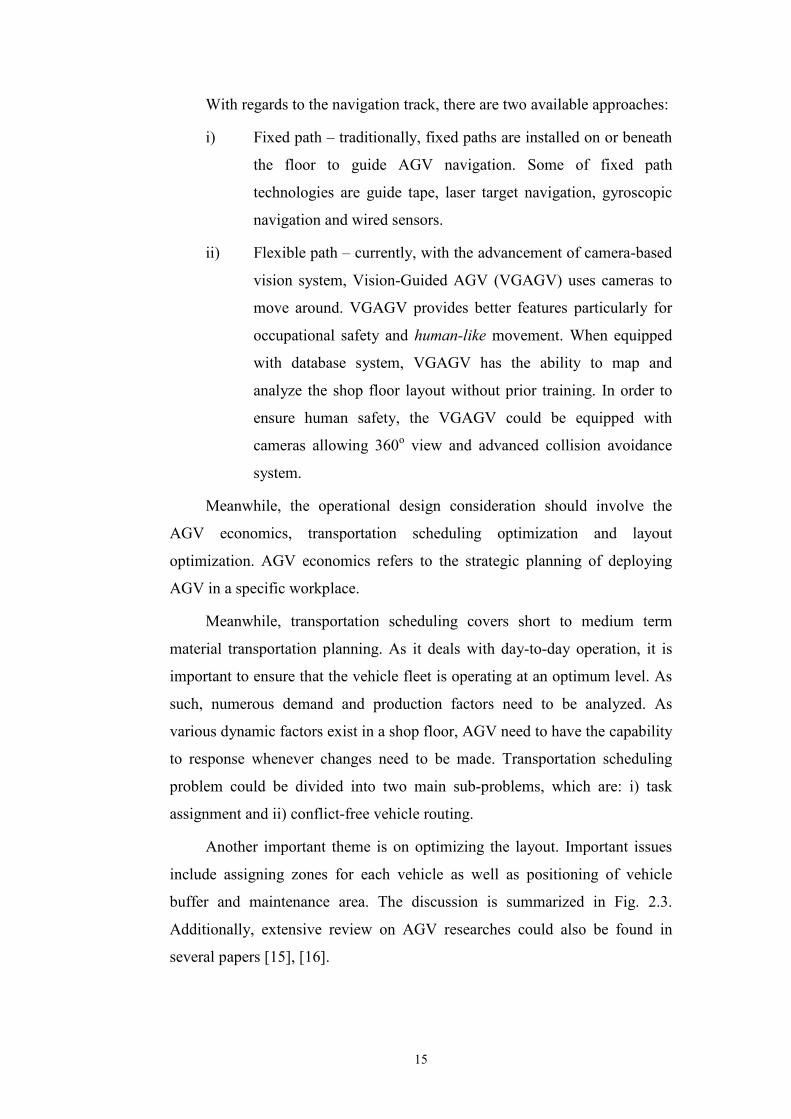
With regards to the navigation track, there are two available approaches:
i) Fixed path – traditionally, fixed paths are installed on or beneath
the floor to guide AGV navigation. Some of fixed path
technologies are guide tape, laser target navigation, gyroscopic
navigation and wired sensors.
ii) Flexible path – currently, with the advancement of camera-based
vision system, Vision-Guided AGV (VGAGV) uses cameras to
move around. VGAGV provides better features particularly for
occupational safety and human-like movement. When equipped
with database system, VGAGV has the ability to map and
analyze the shop floor layout without prior training. In order to
ensure human safety, the VGAGV could be equipped with
cameras allowing 360o view and advanced collision avoidance
system.
Meanwhile, the operational design consideration should involve the
AGV economics, transportation scheduling optimization and layout
optimization. AGV economics refers to the strategic planning of deploying
AGV in a specific workplace.
Meanwhile, transportation scheduling covers short to medium term
material transportation planning. As it deals with day-to-day operation, it is
important to ensure that the vehicle fleet is operating at an optimum level. As
such, numerous demand and production factors need to be analyzed. As
various dynamic factors exist in a shop floor, AGV need to have the capability
to response whenever changes need to be made. Transportation scheduling
problem could be divided into two main sub-problems, which are: i) task
assignment and ii) conflict-free vehicle routing.
Another important theme is on optimizing the layout. Important issues
include assigning zones for each vehicle as well as positioning of vehicle
buffer and maintenance area. The discussion is summarized in Fig. 2.3.
Additionally, extensive review on AGV researches could also be found in
several papers [15], [16].

16
Fig. 2.3. Enabling Technologies for AGV Operation
2.2.3 Scheduling and Routing of Autonomous AGVs using Vehicle
Routing Problem
Generally, AGV scheduling inherits the characteristics of the more
established theory of Vehicle Routing Problem (VRP). VRP is categorized as
a combinatorial optimization problem. Its objective is to delegate
transportation jobs to a fleet of vehicles in an appropriate order so that the
jobs could be completed in time [16]. Typically, transportation cost and time
are also considered in the minimization functions. There are several methods
could be utilized to solve VRP model. Mixed Integer Programming [17], [18],
[19] and heuristic methods [17], [20], [21] are among the most commonly
used to solve VRP and its variants.
Nevertheless, in dealing with autonomous AGVs, there is also a need to
focus on how vehicles could navigate safely. Autonomous AGVs possesses
unique characteristics where their routes may not be controlled by single
centralized controller. Therefore, there is another need to build a conflict-free
routing mechanism. Singh and Tiwari [22] proposed a conflict-free vehicle
routing mechanism based on multi agent architecture.
In this research, a generalized variant of VRP, specifically Vehicle
Routing Problem with Time Windows (VRPTW) has been adopted to
Enabling Technologies for AGV Operation
Operational DesignPhysical Design
Vehicle Design
Navigational Technology
Communication Facilities
AGV Economics Transportation scheduling
Layout optimization
• Mechanical structure • Electrical design • Jigs & fixtures design • Payload capacity
• Architecture design • Information exchange • Data storage
• Navigation track• Traffic control system • Safety requirements
• Communication medium• Communication protocol
• Capacity planning • vehicles requirement
• AGV zone design • AGV coordination
Control Architecture
• Task assignment algorithm
• Vehicle routing

17
implement AGV scheduling. Mathematical approach was used to obtain the
solution.
2.2.4 Performance Measurements of MTS in a Manufacturing Industry
Performance indicators (PIs) are typically utilized to measure the
successfulness of a particular proposed method to achieve stated objectives. It
is important to select appropriate PIs so as to measure critical aspects resulted
from the implemented proposal. Some of the PIs used in this research are
categorized as the following:
i) Related to production performance
• System throughput (STH) refers to the total output produced in a
specific time period. Throughput is defined as the summation of
the jobs completed by the system.
• Average pickup waiting time (AWT) that measures the time
difference between actual vehicle arrival times and the earliest
pickup time.
ii) Related to vehicle performance
• Percentage of fully loaded travel (FLT) that is useful to measure
how AGV’s capacity is used in the experiment.
• Standard deviation of FLT is necessary to analyse the variation of
FLT between vehicles.
• AGV traveling distance that may be used to measure the efficiency
of vehicle utilization.
iii) Related to computational effort required
• Computational time is effective in comparing the required
computational effort in order for the proposed method to obtain
final solutions.

18
2.3 Developing Autonomous Control System based
on Multi Agent Architecture
2.3.1 Principle of Intelligent Agent
Agent is defined as autonomous problem-solving entity, which by nature
continuously senses, communicates and reacts in order to satisfy specified goal
within an operation environment [23], [24]. While the concept of agent has
been viewed from various perspectives, this thesis used the definition by [24]
where essentially, agent could be categorized as the following:
• Purely Reactive Agent should be equipped with sensor to detect
changes in the environment and response accordingly through
actuator as illustrated in Fig. 2.4. Agent’s function is based on
condition-action rule: if-then action where action: E → Ac where E
is the set of environment states and Ac is the set of agent’s actions.
One of an example for the Purely Reactive Agent is thermostat of
which the main purpose is to maintain room temperature by turning
on the heating or cooling system accordingly.
Fig. 2.4. Structure for Purely Reactive Agent [24].
• Agent with Perception – the agent consists of a fairly high level internal
architecture of a reactive agent. Agent’s decision function is separated
into perception and action subsystems. ‘See’ module represents the
agent’s ability to monitor changes in its environment, whereas the
‘action’ module represents the decision making process of the agent
where objective functions could be stored. The output of see function is
based on the mapped environment states where see: E → Per and
Agent
Environment
ActuatorSensor
Input Output

19
action: Per* → A which defines the percepts, Per to actions, A
accordingly. The concept agent is graphically depicted in Fig. 2.5.
Fig. 2.5. Structure for Agent with Perception [24]
• Agent with State – the agent is equipped with internal data structure
that is used to store information. This allows the agent to have better
decision-making capability by changing the agent’s action function. As
the perception function remains see: E → Per, the action-selection
complies to action: I → Ac where I may represents the set of all
internal states. Next function is used to map the internal state and
percept to an internal state as next: I * Per → I. Fig. 2.6 illustrates the
concept.
Fig. 2.6. Structure for Agent with Internal State [24]
Agent
Environment
ActuatorSensor
Input Output
See Action
Next State
Agent
Environment
ActuatorSensor
Input Output
See Action

20
2.3.2 Types of Multi Agent Architecture
The concept of Multi Agent System (MAS) is established when multiple
intelligent agents are systematically planned to cooperate in the same working
environment to achieve specific goal. Essentially, the architecture for multi
agent system (MAS) can be categorized into three main types as the following
[25]:
i) a contract-net system
In a contract-net system, delegation of a composite job among
agents is conducted by establishing contract among themselves.
Typically, multiple jobs are shared among agents within the same
environment leading to the creation of a network of contracts,
hence the name ‘contract-net’. Agent that has job availability
initiates the task-sharing protocol by broadcasting Call for
Proposals (CFP). Agents that received CFP will then bid to offer
the service to the initiating agent. Best bid will be selected and the
winning agent will serve the initiating agent. Details of the
protocol are provided in Section 2.2.3.
ii) specification-sharing system
Specification-sharing system is based on the idea where agents
supply the information regarding their capabilities and needs to the
others. Based on the acquired information, activities are carried out
with mutual understanding. Survey shows limited numbers of
engineering applications are based on specification-sharing system.
Nevertheless, system proposed by [26] could be regarded as
having the attributes of specification-sharing system [27].
iii) federated system
The differences between federated MAS and the other two types
are federated system has hierarchical agent structures where
coordinators are deployed to supervise groups of local agents.
Therefore, local agents only communicate within their federation
while inter-federation communications are carried out by
coordinators.

21
In this research, contract-net architecture is utilized particularly because
i) it is suitable for engineering application with dynamic environment
requiring real-time decision-making capability compared to specification-
sharing system and ii) considering the size of the application, federated
system might not be necessary. As such, communication could be less
complicated and more straightforward.
2.3.3 Fundamental of Contract Net Protocol (CNP)
CNP is one of the communication protocols that are used for tasks
delegation in Distributed Artificial Intelligence (DAI) systems. It was first
introduced by Smith [28]. Due to its efficiency, Foundation of Intelligent
Physical Agents (FIPA) of IEEE [29] has taken it as a standard to formalize
communication protocol particularly between a group of nodes or agents
within a system. Negotiation protocol that is based on Standard CNP (SCNP)
consists of a sequence of four main steps as depicted in Fig. 2.7 [30]. Related
agents must go through the following steps to negotiate each contract:
i. The initiator sends a CFP.
ii. Each participant reviews the CFP and responds accordingly.
iii. The initiator selects participant with the best bid and informs rejection of
other bids.
iv. Selected participant notifies the initiator on task execution.
CNP is a systematic protocol where negotiation could be executed.
Auction mechanism is suitable for allocating resource particularly when the
information of the entire environment is not totally explored. Furthermore,
auction algorithm has excellent computational efficiency and is regarded to be
among the best in optimizing single commodity network problems [31].
However, existing researches focused on the application of CNP to suit
static AGV operational environment making it less suitable to meet the
requirements of dynamic AGV operations. Furthermore current approach does
not fully utilize the latest information within a dynamic system. This leaves
unaddressed technical shortcomings that will restrict realization of an
effective distributed AGV system.

22
Fig. 2.7. Sequence of Contract Net Interaction Protocol
2.3.4 Agent Standards and Interoperability
There are several governing bodies that provide standards for intelligent
agent and MAS. Two of the prominent bodies are the Foundation for
Intelligent Physical Agent (FIPA), a standards organization of IEEE
Computer Society [29] and the Agent Platform Special Interest Group (PSIG),
a subgroup of Object Management Group [32].
FIPA has established 25 specifications as standards for agents system.
The specifications can be categorized under five main themes: agent
communication; agent transport; agent management; abstract architecture; and
applications. FIPA regards agent communication as the core category at the
heart of the FIPA multi-agent system model. Meanwhile, PSIG has more than
10 specifications particularly related to agent-based system modelling.
Initiator Participant
CFP
refuse
propose
reject-proposal
accept-proposal
failure
inform-done
inform-ref
FIPA-Contract Net-Protocol
m
ndeadline
i≤n
j=n-i
k≤j
l=j-k

23
Other standardization bodies include AgentLink III, the European
Coordination Action for Agent Based Computing [33] and US Defense
Advanced Research Projects Agency (DARPA) that came with DARPA Agent
Markup Language (DAML).
2.4 Scheduling of Distributed Resources using
Combinatorial Auction
Combinatorial auctions (CA) refer to a systemic auction procedure that
allows bidders to place a single bid on combinations of discrete items [34]. It
could be employed when auctioneer has more than one item to be offered
simultaneously. Originally utilized in economics and game-theory
applications, there is now a growing number of researches applying the
method to solve engineering problems such as airport slot allocation,
scheduling in multi-rate wireless network, grip computing design and
operating system memory allocation [35], [36], [37].
Compared to the traditional auction approach, CA has advantages on
certain aspects particularly in enabling bidders to evaluate both
complementary and substitutability attributes of the items put on auction. This
could minimize the risks of only obtaining a subset of items that are not worth
as much as the complete set. Based on the evaluation, bidders will then be
able to submit a package of bid for the intended items.
When a bidder participates in auctions consist of multiple auctioneers
with multiple items, the bidder needs the ability to assess the value for each
item. Furthermore, if the bidder intends to bid for more than an item, there is a
need to evaluate the consequences of acquiring an item to the others. Two
important attributes are:
• Complementarity
For a bidder, the value of an item can vary depending on other items
that could be acquired. Thus, there exists complementarity attribute
between items i1 and i2 where bidder a may put a value, v(I) as of the
following:
{ }( ) { }( ) { }( )2121 , iviviiv aaa +>

24
• Substitutability
Another important attribute need to be assessed is on the readiness of
a bidder to accept alternative item should the best item couldn’t be
won. Substitutability can be expressed as the following:
{ }( ) { }( ) { }( )2121, iviviiv aaa +<
Looking from a material transportation viewpoint, both complementarity
and substitutability attributes are critical particularly as tasks assignment will
have consequent route establishment. Optimizing one assignment without
considering others will still result in under optimized vehicle route. This could
be overcome by evaluating multiple jobs simultaneously. As such, CA could
be a suitable method to schedule the operation of autonomous AGVs.
2.5 Key Research Problems
Identification of critical research problems is necessary to ensure the
system will be able to operate efficiently. It is necessary so that specific
research objectives could be determined. The key research problems that have
been studied in the thesis are as the following:
P1) Existing architecture and task assignment protocol does not
consider dynamism of MTS operation. This prevents the entity
from making optimal assignment thus resulting in
underperformance of the entire system. In order to achieve
competitive performance, there is a need for an assignment
protocol that could exploit latest information within the system.
Since transporters are moving entities, it is appropriate for the
protocol to consider the location of transporters in evaluating task
assignment as well as providing mechanism to re-evaluate
assignments made.
P2) Existing researches on distributed-controlled MTS in particular
AGV system don’t contemplate the deployment of vehicle with
multiple-loading capacity. Due to the fact that existing scheduling
mechanism of distributed-controlled AGV is still depending on
single-task allocation per auction, it is less suitable to be utilized

25
when dealing with multi-capacity transporters as it hinders the
entire assignments from being fully optimized where bidders could
not evaluate the complementary or substitutability attributes
among tasks.
P3) Most of the research models for AGV system design used
simplified cases which may be useful to test the implementation of
new idea. However, this might underestimate the effect of some
decisive operation factors. In order to design a realistic AGV
system, it is necessary to consider a realistic production
environment. Furthermore, in a typical industrial environment,
there are multiple operational criteria that need to be handled. As
such, there is a need to determine the best combination of design
variables taking into account related critical operational criteria.
2.6 Summary
The fundamental of important technologies required to develop an
autonomous-controlled AGV system have been reviewed. The details on how
the technologies were employed are explained in the respective chapters.

26
Chapter 3 MAS-Based MTS Architecture using Predictive-Reactive Approach 3.1 Introduction
3.1.1 Overview
Upon finishing the literature review, the trend for state-of-the-art
researches and the corresponding important transportation attributes for
advanced MTS could be extracted. Based on the attributes, key research
problem could then be determined. Taking into account both aspects, an
appropriate MTS control architecture based on MAS architecture could be
proposed. The discussion in this chapter is divided into two main components:
i) Identification of generic attributes required by an advanced MTS
system and existing problems need to be solved to realize it.
ii) Consequently, an autonomous MTS control architecture based on
MAS that is capable to address both perspectives is proposed. The
architecture is focused on enabling the MTS to conduct dynamic
task assignment procedure.
3.1.2 Philosophy of Deploying Distributed and Autonomous MTS
Key philosophy of deploying MAS is to enable each entity the
autonomy in planning and executing their responsibilities. This could be
realized by providing them the intelligence to make decision independently
based on their goal and current environment status. Besides, MAS enable the

27
development of modular design application particularly for information
processing and decision making functions. Compared to conventional MTS
with centralized scheduler, the MAS-based MTS could provide new
perspective as the following:
• Change management is localized – In dealing with dynamic
environment, it is important for the system to continuously monitor the
established schedule and dictate changes upon necessary. The
drawback of conventional method is that minor changes may affect the
transportation schedule of the whole fleet. Agent-based MTS minimize
the impact chain by localizing the change only to the related machines
and vehicles thus minimizing system nervousness.
• Information traffic load and processing is localized – Compared to the
traditional system with centralized decision maker (CDM) that
requires system-wide information, the proposed MAS approach
consists of multiple decision makers (DM). This enables the
information traffic to be localized within a specific DM thus eliminates
the need for a decision maker to process unneeded information.
• Eliminate single-point failure – This will increase the entire system
fault-tolerant capability. As the entities have the autonomy in making
decision, any failure could be isolated.
3.1.3 Realizing Dynamic Task Assignment based on Predictive-Reactive
Approach
In a realistic world, scheduling or task assignment is a continuous and
ongoing process. This is due to the fact that more often than not, established
initial plan need to be revised due to the changing circumstances cause by
various dynamic factors. While initial plan could be derived using predictive
scheduling, the process of revising an earlier schedule triggered by dynamic
events is termed as reactive scheduling.
Predictive-reactive scheduling is regarded as the most widely used
approach to manage dynamic factors within a manufacturing system [38]. It
refers to scheduling and re-scheduling processes where initial schedule could
be amended as a response to real-time event. This chapter aims to provide a
28
task assignment protocol inheriting predictive-reactive characteristics that also
has the function to react to dynamic events related to AGV operation.
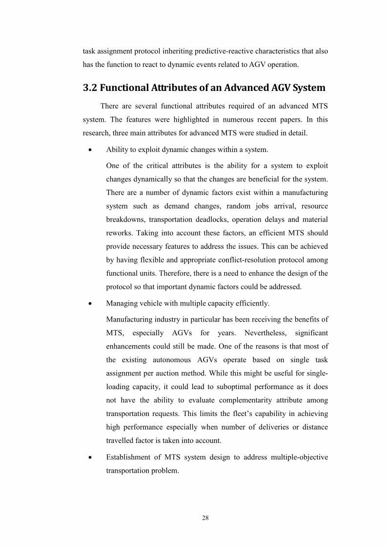
3.2 Functional Attributes of an Advanced AGV System
There are several functional attributes required of an advanced MTS
system. The features were highlighted in numerous recent papers. In this
research, three main attributes for advanced MTS were studied in detail.
• Ability to exploit dynamic changes within a system.
One of the critical attributes is the ability for a system to exploit
changes dynamically so that the changes are beneficial for the system.
There are a number of dynamic factors exist within a manufacturing
system such as demand changes, random jobs arrival, resource
breakdowns, transportation deadlocks, operation delays and material
reworks. Taking into account these factors, an efficient MTS should
provide necessary features to address the issues. This can be achieved
by having flexible and appropriate conflict-resolution protocol among
functional units. Therefore, there is a need to enhance the design of the
protocol so that important dynamic factors could be addressed.
• Managing vehicle with multiple capacity efficiently.
Manufacturing industry in particular has been receiving the benefits of
MTS, especially AGVs for years. Nevertheless, significant
enhancements could still be made. One of the reasons is that most of
the existing autonomous AGVs operate based on single task
assignment per auction method. While this might be useful for single-
loading capacity, it could lead to suboptimal performance as it does
not have the ability to evaluate complementarity attribute among
transportation requests. This limits the fleet’s capability in achieving
high performance especially when number of deliveries or distance
travelled factor is taken into account.
• Establishment of MTS system design to address multiple-objective
transportation problem.

29
MTS system design is a crucial issue particularly as it requires huge
capital investment. In order to provide a realistic MTS system design,
it is necessary to consider a realistic industrial environment.
Furthermore, in a typical industrial environment, there are multiple
operational criteria that need to be handled. As such, there is a need to
determine the best combination of design variables.
3.3 Development of Autonomous MTS
Architecture based on MAS
Based on the discussion on the required attributes and related problems
in realizing an advanced MTS, this section proposes an MTS control
architecture based on MAS.
3.3.1 Fundamental of MAS
In this thesis, intelligent agent is defined as a goal-oriented autonomous
computational entity, which continuously senses, communicates and reacts
accordingly within an operation environment [39]. As such, each entity is
equipped with a certain degree of learning ability and is responsible in making
decisions on behalf of a respective physical entity in a manufacturing system.
Meanwhile, the concept of MAS arises when multiple agents are
systematically planned to cooperate in the same working environment to
achieve specific goals. In establishing appropriate MAS, there are four main
agent elements that need to be planned:
i. Multi-agent system architecture.
ii. Definition of agent’s functionality.
iii. Communication protocol for executing jobs.
iv. Agent’s reward system consisting bidding functions.
Fundamental MTS operational control of task assignment and routing
are mapped into the MAS framework. Task assignment is executed using
auction-based negotiation protocol between agents. In order to provide a
certain degree of freedom for the transporters to plan and decide its own
operation, the agent-based control system is embodied into each vehicle.

30
In order to establish a distributed architecture for MTS operation, it is
necessary to identify the task assignment requirements. Fig. 3.1 summarizes
the stages of material transportation planning and the proposed task
assignment method. This research uses job shop machine schedule as the
system input.
Fig. 3.1. Proposed Task Assignment Method within Material
Transportation Planning
The central idea to establish transportation assignment is by utilizing
auction-based protocol to handle task assignment procedure. Based on
standard Contract Net Protocol (CNP), an Improved CNP (ICNP) is proposed
Transportation Tasks Owner Agents
Transporter Agents
Monitor and Coordinate Agents
• Responsible to transport material
• Minimize atvi
• Conduct auction for tasks need to be transported
• Monitor system • Collect data• Coordinate data
sharing (e.g.: AGV position)
Improved CNP with:•Location-aware•Event-driven multi round bidding•1-to-n communication constraint
Auction protocol
Ideal Transportation Requirement
Assigned tasks
Material Transportation Plan
Vehicle Routing & Conflict Resolution
Conflict-free vehicle route
Task Assignment
• Minimize waitp
31
in order to enhance communication protocol between Transporter Agent and
Transportation Tasks Owner Agent to accommodate the procedure.
ICNP is equipped with event-driven multi-round proposal capability and
the communication is conducted in a bounded communication range. Apart
from Transporter Agent and Transportation Tasks Owner Agent, Monitor and
Coordinate Agent is deployed to monitor and to ensure the system operates
efficiently. In realizing the entire mechanism, multi-agent architecture is
proposed.
3.3.2 Proposed MAS Architecture for Autonomous MTS
There are variations of agent-based control architecture applied for task
assignment purpose [23], [40], [41], [42]. However, most of the architectures
were not based on auction mechanism and are developed to suit static
environment. Thus, a unique multi-agent architecture is needed to satisfy the
complete set of requirements for distributed MTS operation.
Basically there are three types of agent deployed within the system
namely as Transporter Agent, Transportation Tasks Owner Agent and Monitor
and Coordinate Agent. All of the agents are equipped with specific set of
functions. Related notations are shown in Table 3.1.
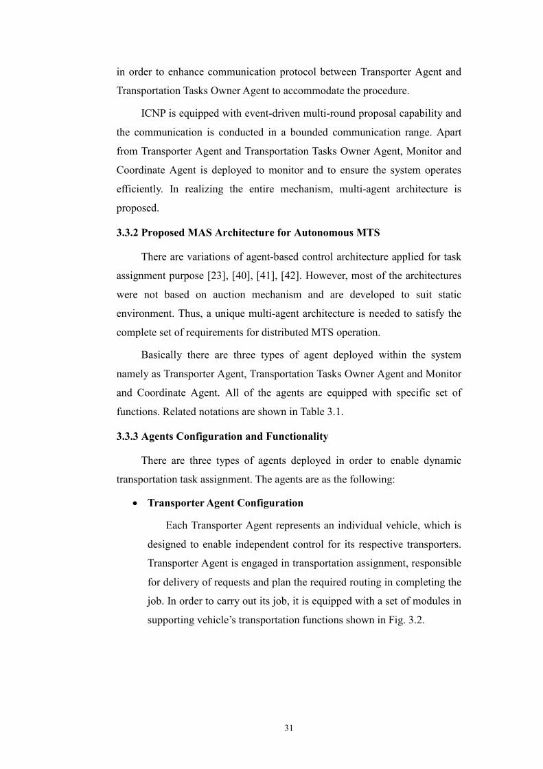
3.3.3 Agents Configuration and Functionality
There are three types of agents deployed in order to enable dynamic
transportation task assignment. The agents are as the following:
• Transporter Agent Configuration
Each Transporter Agent represents an individual vehicle, which is
designed to enable independent control for its respective transporters.
Transporter Agent is engaged in transportation assignment, responsible
for delivery of requests and plan the required routing in completing the
job. In order to carry out its job, it is equipped with a set of modules in
supporting vehicle’s transportation functions shown in Fig. 3.2.
32
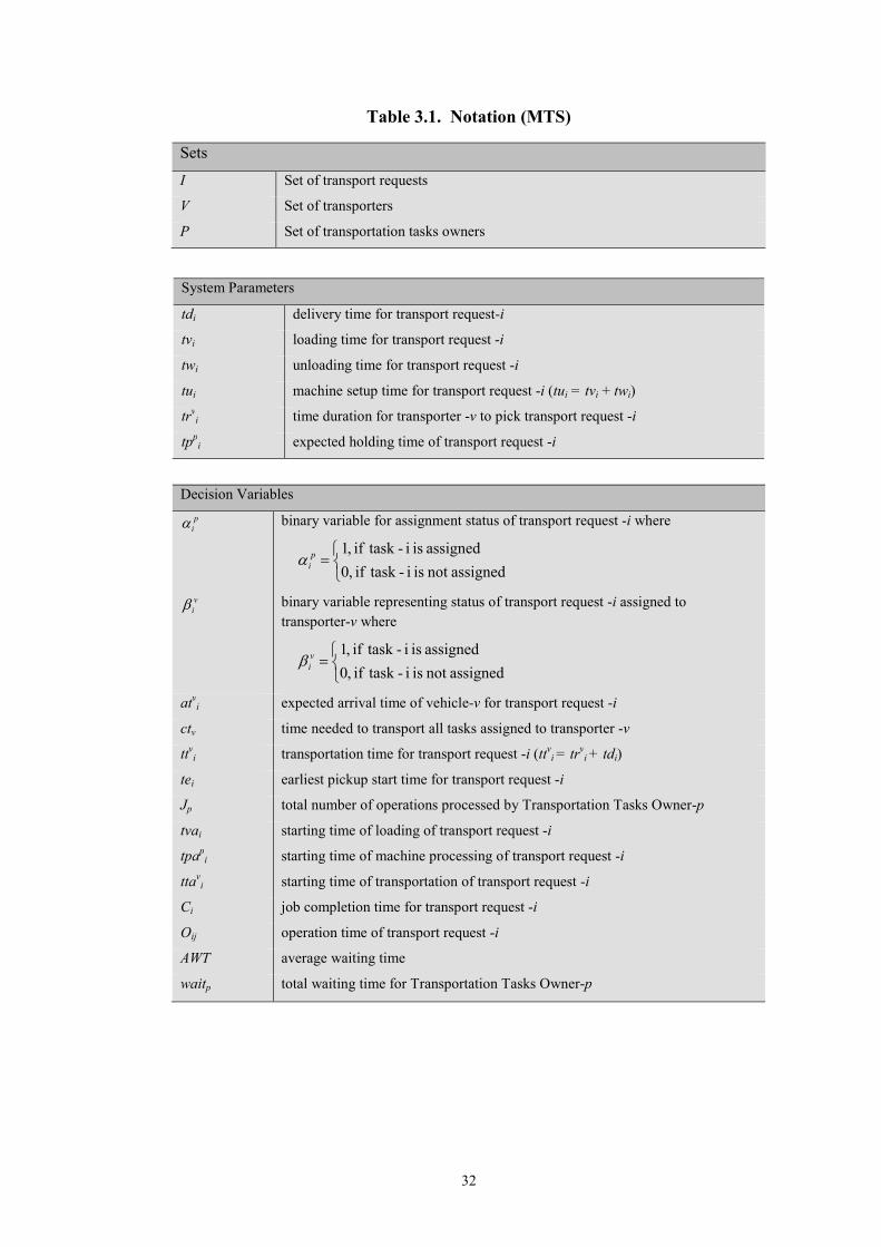
Table 3.1. Notation (MTS)
Sets
I Set of transport requests
V Set of transporters
P Set of transportation tasks owners
System Parameters
tdi delivery time for transport request-i
tvi loading time for transport request -i
twi unloading time for transport request -i
tui machine setup time for transport request -i (tui = tvi + twi)
trvi time duration for transporter -v to pick transport request -i
tppi expected holding time of transport request -i
Decision Variables
piα binary variable for assignment status of transport request -i where
= assignednot is i- taskif ,0
assigned is i- taskif ,1 p
iα
viβ binary variable representing status of transport request -i assigned to
transporter-v where
= assignednot is i- taskif ,0
assigned is i- taskif ,1 v
iβ
atvi expected arrival time of vehicle-v for transport request -i
ctv time needed to transport all tasks assigned to transporter -v
ttvi transportation time for transport request -i (ttv
i = trvi + tdi)
tei earliest pickup start time for transport request -i
Jp total number of operations processed by Transportation Tasks Owner-p
tvai starting time of loading of transport request -i
tpapi starting time of machine processing of transport request -i
ttavi starting time of transportation of transport request -i
Ci job completion time for transport request -i
Oij operation time of transport request -i
AWT average waiting time
waitp total waiting time for Transportation Tasks Owner-p

33
Fig. 3.2. Agent configuration for Transporter Agent
Task assignment and vehicle routing are the two main functions
that need to be established in order to have an efficient MTS.
Conventionally, both aspects can be planned sequentially with task
assignment function precedes the vehicle routing function where the
output of task assignment is used as the input for vehicle routing.
Based on our survey, vehicle routing has been well studied by other
researchers. Thus, this research opted to focus the improvement on job
assignment problem and adopted vehicle routing method proposed by
Singh and Tiwari [22].
In order to support autonomous vehicle operation, dedicated
agent configuration equipped with required sub-modules has been
designed. Transporter Agent has the capability to decide on which
operation should be selected for delivery based on some specific
criteria. In serving transportation request, the agent will attempt to
achieve its main objective that is to minimize its arrival time for task it
is bidding for. Upon receiving Calls for Proposal (CFP), each agent
determines its atvij to pick-up the announced task as defined in (Eq. 3.1)
to (Eq. 3.5) where trvij represents time duration needed for the vehicle
to retrieve the offered task; ctv is the time needed to complete the
transportation of all tasks assigned to transporter-v. Furthermore, i
refers to a transportation request need to be moved.
Sensed data
Updated information
Focus Data
Transporter Agent
Communication Interface
MessageExchange
Main Functions
Bid Generation
RoutingSensing Interface Output
Input
Transporter Database
Layout
Tasks Info Vehicle Info
Bid Info
Info input & retrieval
Sensed data
Updated information
Focus Data
Transporter Agent
Communication Interface
MessageExchange
Main Functions
Bid Generation
RoutingSensing Interface Output
Input
Transporter Database
Layout
Tasks Info Vehicle Info
Bid Info
Transporter Database
Layout
Tasks Info Vehicle Info
Bid Info
Info input & retrieval
Enviro
nment

34
Min viat .................................................... (3.1)
s.t. vv
ivi cttrat += ................................ (3.2)
( )[ ]∑=
++++=I
i
viiii
vi
viv twtvtdtrttact
1
)()( β (3.3)
,1=viβ i∀ ........................................... (3.4)
vv
i cttr > .............................................. (3.5)
• Transportation Tasks Owner Agent Configuration
Transportation Tasks Owner Agent represents the interest of task
owners and equip them with decision making capability. The agents
with configuration as in Fig. 3.3 are responsible to initiate CFP,
evaluate bids and assign delivery task to the most suitable vehicle.
Essentially its main objective is to maximize the overall throughput.
Therefore, Transportation Tasks Owner Agent have the ability to
decide which participant should be awarded with the contract. In
achieving the objective, the agents are equipped with a set of decision-
making modules to evaluate the decision criteria.
Fig. 3.3. Agent configuration for Transportation Tasks Owner Agent
This research proposes an Improved CNP (ICNP) to manage
two important dynamic factors in AGVs operation. The factors are:
i) dynamic status of vehicle’s capacity availability
Sensed data
Updated information
Focus Data
Transportation Tasks Owner
Agent
Communication Interface
MessageExchange
Main Functions
Initiate Auction
Winner Determination
Sensing Interface Output
Input
Task Owner Database
Tasks Info
Auction Info
Info input & retrieval
Sensed data
Updated information
Focus Data
Transportation Tasks Owner
Agent
Communication Interface
MessageExchange
Main Functions
Initiate Auction
Winner Determination
Sensing Interface Output
Input
Task Owner Database
Tasks Info
Auction Info
Info input & retrieval
Environment

35
ii) the positioning advantage of certain vehicles in
handling a particular transportation request.
As such, Transportation Tasks Owner Agent is equipped with the
modules to support both requirements. The details are discussed in
Chapter 4. Transportation Tasks Owner Agents are also responsible for
interacting with TA to update job completion status and to receive
production orders from production management system.
Transportation Tasks Owner Agent is responsible to minimize
waitp for all of the tasks as defined in (Eqs. 3.6 and 3.7) and average
load-pickup waiting time for each operation (AWT) as in (Eq. 3.8) are
used as the performance indicators where tvai is the loading start time
of transport request-i which is also the actual starting time of loading
operation.
Min pwait ............................................... (3.6)
s.t. ∑=
−=I
i
pii
vip tetvawait
1
)( α ................ (3.7)
=∑
= p
pP
p J
waitAWT
1
............................... (3.8)
• Monitor and Coordinate Agent Configuration
Since agents store information, plan and react based on local
knowledge, it lacks an entire view on the system. Hence, there is a
need to establish an approach on how to trace system operation and
performance. An agent needs to be assigned to take charge on these
functions. Monitor and Coordinate Agent as illustrated in Fig. 3.4,
resides at a monitoring base i.e. a dedicated computer located in shop
floor.
Fundamentally, the agent is responsible to monitor the entire
Transportation Tasks Owner Agents and Transporter Agents. This
could further facilitate any fault-tolerant mechanism to solve machine
or vehicle failure. Additionally, Monitor and Coordinate Agent
responsibles to provide Transportation Tasks Owner Agent the

36
information of transporters that are eligible to bid for a specific
transport request. The detail is discussed in Chapter 4.
Moreover, Monitor and Coordinate Agent also stores system
data such as job input and output data. Monitor and Coordinate Agent
may interacts with Transportation Tasks Owner Agent and Transporter
Agent during task assignment process. In addition, Monitor and
Coordinate Agent holds job completion time, Ci which can be
expressed as in (Eq. 3.9) and (Eq. 3.10) where Oi refers to the
operation time for ith job.
∑=
=I
iii OC
1
................................................. (3.9)
vi
vi
pi
pi
piii tttptuO βαα ++= ................... (3.10)
Practical-wise, in order to avoid single-point failure, mirror agent
of Monitor and Coordinate Agent need to be established in a replicated
monitoring base as a backup. Both agents possess the same functions,
are connected and synchronized with each other at a specified time
interval.
Fig. 3.4. Agent configuration for Monitor and Coordinate Agent
Sensed data
Updated information
Focus Data
Monitor and Coordinate Agent
Communication Interface
MessageExchange
Environment
Main Functions
Transporter Monitoring
Task MonitoringSensing Interface
Output
Input
TA Database
Task Owner Info
Tasks Info
Info input & retrieval
Task Owner Monitoring
Transporter Info

37
3.4 Key Research Objectives and Approaches
In developing efficient MAS for MTS, key research objectives have been
determined. Consequently, necessary approaches to fulfill the objectives have
been identified. The discussion is summarized in Table 3.2.
Table 3.2. Key research objectives and approaches
Section 3
Dynamic Protocol Section 4
Multi Loading Capacity Section 5
System Design
Key
Obj
ectiv
es
To enhance Contract Net Protocol (CNP) to: 1.Exploit dynamism of AGV position 2.Enable revisable bidding
To enhance task assignment protocol to: 1. Optimize the performance of multi-load AGV 2. Assign multiple tasks per auction through multi-initiator to multi-participant communication
To provide an effective tool to decide design parameter of MAS-based AGV system for dominance-based multi-objective problem.
Mai
n A
ppro
ache
s
Enhance CNP with: 1. Location-aware 2. Utilize Monitor and Coordinate Agent to facilitate location-aware protocol 3. Event-based multi-round bidding features 4. Modify time constraint to realize event-based bidding
1. Formalize Knapsack Problem model to optimize utilization of AGV loading capacity 2. Extend Vehicle Routing Problem with Time Window for Multi-Load AGV 3. Utilize Combinatorial auction with Exclusive OR (XOR) bidding rule 4. Introduce Auction Agent to resolve task assignment conflicts
Establish simulation approach of MAS-based AGV system design: 1. Provide simulation procedure & tool of the MAS-based AGV system 2. Utilize RSM method for optimizing design parameters’ values
3.5 Summary
This chapter has laid the foundation of an advanced Vehicle-based
Material Transportation System. MAS-based MTS control architecture is used
to realize the system. The architecture will be used in the following discussion.

38
Chapter 4
Enhancement of CNP with
Location-Aware and Event-
based Multi Round Bidding
Features
4.1 Introduction
For years, majority of the researches in AGV scheduling has been based
on centralized planning method. In a centralized approach, schedule for the
entire fleet is planned by a single decision-maker that has all of the system
information. While the approach typically possesses the advantages of global
optimization capability, the method comes with major shortcomings as well.
Occasionally, centralized method becomes very difficult to cope with
unforeseen circumstances such as unexpected express requests and machine
breakdown as it takes long computation time to obtain the route planning of
large scale systems [43], [44], [45].
Looking from MTS point of view, AGV system is made up of several
functional units that are operating independently, thus each may have their
own preferences in achieving the objective function. This emulates the
concept of independent units that should be given certain degree of freedom to
decide whether to cooperate with other units or not. Therefore, it is not

39
necessary for one individual vehicle to share all their information (such as
tasks currently assigned, battery level etc.) in case cooperation is not needed.
This contradicts the characteristics of centralized control that requires
information of the entire system prior to the computation.
In addressing dynamic and real-time operation criteria, this chapter
introduces a distributed task assignment method for autonomous AGV based
on auction method. Multi agent system (MAS) as proposed in Chapter 3 is
employed to realize the distributed environment and Contract Net Protocol
(CNP) is used to facilitate auction-based task assignment method.
The discussion in this chapter is focus on the development of an
improved protocol to exploit dynamic transportation factors within the system
and to overcome existing limitation.
4.2 MAS Architecture for Autonomous AGV
4.2.1 Overview
As there are several approaches of developing MAS architecture for task
assignment and scheduling, there is a need to clarify the architecture that is
needed to fulfill the requirements of a dynamic AGV system that operates
within a manufacturing environment. A unique system architecture has been
established in this research in order to map AGV control requirements into the
agent-based framework. As discussed in Chapter 3, there are three agent types
needed for MTS. In order to adapt the idea for AGV system, basically there
are three types of agent deployed within the system namely as:
• AGV Agent (AGVA) that responsible as Transporter Agent.
• Machine Agent (MA) that responsible as Transportation Tasks
Owner Agent.
• Monitor and Coordinate Agent (TA).
The respective agent strcutures are shown in Fig. 4.1 The related
functions stated in Chapter 3 have been modified accordingly to suit specific
problem case requirement. As such, the notations shown in Table 4.1 will act
as the guide for the entire dissertation.

40
Fig. 4.1 (a) AGVA structure
(b) MA structure
(c) TA structure
Sensed data
Updated information
Focus Data
AGV Agent
Communication Interface
MessageExchange
Environment
Main Functions
Bid Generation
Routing Sensing Interface Output
Input
AGVA Database
Layout
Tasks Info AGV Info
Bid Info
Info input & retrieval
Sensed data
Updated information
Focus Data
AGV Agent
Communication Interface
MessageExchange
Environment
Main Functions
Bid Generation
Routing Sensing Interface Output
Input
AGVA Database
Layout
Tasks Info AGV Info
Bid Info
AGVA Database
Layout
Tasks Info AGV Info
Bid Info
Info input & retrieval
(a)
Sensed data
Updated information
Focus Data
Machine Agent
Communication Interface
MessageExchange
Environment
Main Functions
Initiate Auction
Winner Evaluation
Sensing Interface Output
Input
MA Database
Machine Info
Tasks Info
Auction Info
Info input & retrieval
Sensed data
Updated information
Focus Data
Machine Agent
Communication Interface
MessageExchange
Environment
Main Functions
Initiate Auction
Winner Evaluation
Sensing Interface Output
Input
MA Database
Machine Info
Tasks Info
Auction Info
Info input & retrieval
(b)
Sensed data
Updated information
Focus Data
Monitor and Coordinate Agent
Communication Interface
MessageExchange
Environment
Main Functions
AGV Monitoring
Task MonitoringSensing Interface
Output
Input
TA Database
AGV InfoTasks Info
Info input & retrieval
Machine Monitoring
Ideal Machine Schedule
Sensed data
Updated information
Focus Data
Monitor and Coordinate Agent
Communication Interface
MessageExchange
Environment
Main Functions
AGV Monitoring
Task MonitoringSensing Interface
Output
Input
TA Database
AGV InfoTasks Info
Info input & retrieval
Machine Monitoring
Ideal Machine Schedule

41
Table 4.1. Notation
Sets
IJ Set of operations
A Set of agents
B Set of bids
X Set of AGVs
M Set of machines
L Set of lanes/ arcs/ ordered pair of vertices
T Set of time periods
System Parameters
tdij delivery time for operation-ij
tvij loading time for operation-ij
twij unloading time for operation-ij
tuij machine setup time for operation -ij (tuij = tvij + twij)
trxij time duration for AGV to pick operation-ij
tpmij machine processing time of operation-ij
dxij shortest node-to-node distance to transport load-ij
sd cost for AGV to travel for a unit length
cpx Total loading capacity of AGV-x
pij Pickup station for operation-ij
eij Destination station for operation-ij
Binary Variables
mijα binary variable for assignment status of operation-ij where
= assignednot is ij-operation if ,0
assigned is ij-operation if ,1 m
ijα
xijβ binary variable representing status of operation-ij assigned to AGV-x where
= assignednot is ij-operation if ,0
assigned is ij-operation if ,1 x
ijβ
xmce binary variable representing either AGV-x is capable to carry new load
when it is at machine-m where

42
<
==
if ,1
if ,0
xaxa
xaxaax cpcc
cpccce
xmnδ
binary variable assigned to AGV-x where
= otherwise if ,0
n- tom-node from x travels-AGV if ,1 x
mnδ
xbξ binary variable representing status of bid-b
= otherwise if ,0
bid optimal theis bid active theif ,1xbξ
Decision variables
atxij expected arrival time of vehicle-x for operation-ij
ctx time needed to transport all tasks assigned to AGV-x
ttxij transportation time for operation-ij (ttx
ij = trxij + tdij)
teij earliest pickup start time for operation-ij
tlij latest delivery start time without delaying the entire job sequence
rtj released time of job-j
mtj remaining time of the respective job-j
dtj due time of job-j
Jm total number of operations processed by machine-m
tvaij starting time of loading of operation-ij
tpamij starting time of machine processing of operation-ij
ttaxij starting time of transportation of operation-ij
Ci job completion time
Oij operation time of operation-ij
ccxm current occupied capacity of AGV-x at machine-m
clxm quantity of pickup / delivery for AGV-x at machine-m
adxij difference between teij and AGV’s atx
ij.
qm quantity of transportation request (loading or unloading) at machine m.
ctx time needed by AGV to complete the transportation of all loaded tasks.
tbij end of bidding time for operation-ij
tnij end of bid evaluation time for operation-ij
taij end of auctioning time for operation-ij

43
tpbm,ij end time of processing of operation –ij
Performance Variables
PLT percentage of average loaded travel
loadedx percentage of loaded travel for AGV-x
AWT average waiting time
waitm total waiting time for machine-m
STH system throughput
TOT total production time
fs vehicle fleet size
4.2.2 Agents Functionality
Functionalities for the agents stated are as follows:
i) AGV Agent (AGVA)
AGVA will attempt to minimize its arrival time in serving the
transportation request it is bidding for. As the agent received Calls for
Proposal (CFP) from MA, each AGVA determines its atxij to pick-up
the announced task as defined in (Eq. 4.1) that consists of trxij that
represents time duration needed for the AGV to retrieve the offered
task and ctx that refers to the time needed to complete the
transportation of all tasks assigned to AGV-x. Furthermore, i refers to
a job and j refers to a machine operation belong to the job. The
function and related constraints are stated in (Eq. 4.1) to (Eq. 4.5).
Min xijat .................................................... (4.1)
s.t. xx
ijxij cttrat += ................................ (4.2)
( )[ ]∑∑= =
++++=I
i
J
j
xijijijij
xij
xijx twtvtdtrttact
1 1
)()( β (4.3)
,1=xijβ ji,∀ ....................................... (4.4)
xx
ij cttr > .............................................. (4.5)

44
ii) Machine Agent (MA)
MAs are deployed on all machines to equip the machines with
decision making capability. The agent is responsible to minimize waitm
for each tasks auction as defined in (Eqs. 4.6 and 4.8).
Min mwait .............................................. (4.6)
s.t. ∑∑= =
−=I
i
J
j
mijij
xijm tetvawait
1 1
)( α ......... (4.7)
=∑
= m
mM
m Jwait
AWT1
.............................. (4.8)
iii) Monitor and Coordinate Agent (TA).
TA is equipped with the function set defined in (Eqs. 4.9 and 4.10).
∑∑= =
=I
i
J
jiji OC
1 1
............................................ (4.9)
xij
xij
mij
mij
mijijij tttptuO βαα ++= ............... (4.10)
4.3 Addressing Dynamic Operation Environment
using an ICNP
4.3.1 Requirements of CNP for Autonomous AGV Control
In order to realize an efficient distributed AGV control that is capable to
suit high-performance production environment, it is necessary to define the
characteristic of its communication requirement. The requirements include:
R1. SCNP is based on open-auction concept where all participants receive
CFP and can bid for the task. While AGVs are moving entities, it is
appropriate that task auction should only be made to the vehicles in
acceptable position to bid for the task. SCNP does not fully address
dynamism of AGV operation especially dealing with moving entities.
The fact that the protocol does not take into account AGV location
parameter makes it less capable to exploit possible advantage situations.
R2. The protocol only allows single-round bidding. Bids evaluation will be
made and contract will be awarded at the end of a single bidding period.

45
No revision could be made even if other participants are able to place
better bid thereafter. This handicaps the protocol to exploit system’s
dynamism and make use of the latest information.
Therefore, this chapter proposes an integrated approach to fulfill the
requirements discussed to enable distributed AGV’s dynamic task assignment
mechanism. Specific approach has been laid out to solve each of the
requirements categorically.
4.3.2 Location-Aware Broadcasting of Transportation Request
Availability
i) Location-Aware Task Announcement Broadcasting
One of the important dynamic factors need to be taken into account is
regarding the vehicles’ positions. Therefore, prior to have multi-pass bidding
function, it is necessary that the proposed enhanced protocol has the feature to
distinguish bidders within strategic location from the entire fleet. There are
three main notable merits justifying the establishment of communication
boundary in solving AGV task assignment problem:
• AGV operations occasionally deal with various uncertainty issues
especially from timing perspective. One of the factors is due to the range
of distance involves. There are possibilities that a vehicle may be
blocked, delayed at a control point due to other’s failure or totally
breakdown. Limiting announcement coverage indirectly ‘filters’
potential recipients of the CFP. Therefore, only AGVs within strategic
distance will be involved in the auction. This is important especially
when dealing with large vehicles group.
• There are possibilities that more than one delivery operations are offered
at the same time. Having an unlimited communication range would
burden any single agent with unnecessary information processing tasks
particularly from initiators that are not located within strategic distance
to the vehicle.
• In terms of operational efficiency, it is good to localize AGV movement
within a certain range of distance. Limiting the communication area
could contribute towards localizing AGV to a specific area for most of

46
its time without totally restricting the vehicle to retrieve loads from
different area if necessary.
However, there are also few demerits of employing bounded
communication range as the condition may exposes MAs to several
possibilities that may lead to lower performance. Among the possibilities
include that:
• Since the CFP is only broadcasted within a specified communication
range, most probably not all will receive the CFP. There is a possibility
that any of the missed AGV could provide better solution compared to
the vehicles that received CFP. This is particularly true if wide variation
of performance measures such as AGV- CFP response time is taken into
consideration.
• At any time, there could be no AGV is located within the
communication range to response to the CFP announcement. In this case,
MA has to wait until an AGV travels into its announcement range. This
situation might delay the assignment as well as the actual pickup time.
Nevertheless, in our opinion, the merits possess more significant impact
on the system compared to the demerits. As such, bounded communication
range is applied by introducing location-aware algorithm to identify strategic
vehicles before CFP is made.
In order to conduct a task assignment that is sensitive to the positions of
the respective vehicles, the Initiator (MA) needs to enquire TA on the eligible
candidates (AGVA) to receive the CFP. TA executes an algorithm to
distinguish potential bidders based on their respective locations. The detail
will then be send to the related MA. This is carried out before CFP is initiated.
The communication sequence is depicted in Fig. 4.2 while the Determine
Eligible AGV algorithm is as the following:
Step 1. Obtain current coordinate of AGV-x (lxx, lyx).

47
Step 2. Calculate the distance, dcx between the pick-up station, pij and
each AGV-x based on the Euclidean distance formulation as
the following: ( ) ( )xpijxpijx lylylxlxdc −+−=
Step 3. Determine the AGVs within specified broadcast range, brm:
dcx ≤ brm.
Step 4. End
Fig. 4.2. Sequence diagram to identify potential CFP recipients.
ii) Communication Setup for Practical Application
Practical-wise, there are some points of discussion in employing the
communication system in a production floor. Both wired and wireless
networks could be utilized simultaneously. Wired network could be used to
establish connection between Production Management System (PMS) to MA
and MA-MA connections.
Wireless local area network (WLAN) is used as part of the agent
communication platform particularly to accommodate AGVA-AGVA and
AGVA-MA communications. In having WLAN platform, the message
distance could be bounded to the coverage of IEEE 802.11 standard. Fig. 4.3
illustrates an example of agents’ communication range.
MA TA
Request Eligible AGV
Determine Eligible AGV
Inform Eligible AGV
AGVA
Request AGV Position
Inform AGV Position
<MA_ID, lxpij, lypij>
<AGV_ID, lxx, lyx>
<AGVA_ID, lxx, lyx>
<TA_ID, RequestPosition>

48
Communication range of AGVA Communication range of MA
M1
M3 M4
M1
M3 M4
M2
V1
V2
Fig. 4.3. Agents’ communication range.
There is a concerning issue whenever bounded communication range is
used particularly regarding the possibility to have an overlapped
communication ranges. Since MA represents a machine, the entire system
consists of multiple MAs which in turn could be multi initiators thus
establishing a multi-initiators and multi-participants scenario. In order to
avoid conflict, the system is designed so that AGV could only involve in one
auction at a time. Once an AGV received broadcasted CFP, it will commit to
the auction until the receiving of tentative reject message from MA or until it
completes the delivery assigned.
iii) Locating and Updating the Positions of AGVs
Determination of an AGV position is closely related to the technology
utilized for vehicle navigation system. As such, in order to explain the
possible approaches to determine AGV positions, there may be necessary to
include the discussion on the navigation system as well. Generally, the
mechanisms can be categorized into three approaches as the following:
a. Vehicle-independent positioning system based on Inertial navigation
system.
An inertial navigation system (INS) is a navigation system that uses
a combination of computer (installed on-board of AGV), motion

49
sensors (accelerometers) and rotation sensors (gyroscopes) to
continuously calculate the position, orientation, and velocity of the
AGV via dead reckoning without the need for external references.
b. Wireless Approach
o Local Positioning System (LPS)
Local Positioning System (LPS) is a navigation system that
provides location information within a specific area. Specific
LPS that can be used for locating the AGV position is the Real-
time Locating System that allows real-time tracking of an
object. For the implementation within a factory, LPS may uses
a set of beacons as the communication medium that include
Wi-Fi access points or cellular base stations for communication
purposes.
o Laser Target Navigation
Retro-reflective tapes usually mounted on walls are used as the
guide path. The AGV carries a laser transmitter and receiver on
a rotating turret. The laser is sent off then received again the
angle and distance could be calculated automatically and stored
into the AGV’s memory. The AGV has reflector map stored in
memory and can correct its position based on errors between
the expected and received measurements. It can then navigate
to a destination target using the constantly updating position.
c. Fixed Path-Equipped Vehicle Positioning System
Sensors-Equipped Path: Wire-based navigation guidance is one of
the oldest forms of AGV guidance. Usually, various types of sensor
such as proximity and magnetic sensors could be used to track the
position of an AGV.
4.3.3 Enabling CNP with Multi-Round Bidding
In realizing the protocol, there are two conditions in which task auction
function would be invoked. The first condition is upon availability of any
delivery task. In the context of this research, it would be triggered at the start
of a machine process. MA is responsible to identify and broadcast messages to

50
vehicles currently located within a specific distance to the machine. Then, the
task auction will be conducted based on the proposed protocol.
The second condition is upon the availability of a vehicle. AGV that has
just become available would announce its availability to machine agents.
Should there be any available task waiting to be delivered, MA will send CFP
of the task to the respective vehicle. AGV agent (AGVA) could then bid for
the task.
Consider a situation where AGV v1 (represented by AGVA_1) is
transporting task t1 to machine m1 (represented by MA_1). In addition to that,
t2 at m2 (represented by MA_2) has been tentatively assigned to v1. While v1 is
still moving towards m1, v2 becomes available as it travels into m2
communication range. It may provide better service by having earlier atx,ij. In
this case, modified CNP allows v2 to bid for t2 provided that it is still within
auction period. If the latter bid is better than the earlier bid offered by
AGVA_1, then MA_2 may change the decision and award the contract to
AGVA_2. This facilitates the interacting agents to look for the best solution
available for each task. Fig. 4.4 shows the improved protocol (ICNP).
In order to call for proposals, Initiator (MA) will send delivery task
specification. The analogy of the specification is SEND [OperationID] FROM
[pij] TO [eij] WITHIN TIME [teij, tlij]. Bidders (AGVAs) will reply the CFP by
providing earliest expected arrival time (to start pickup the task), atxij and its
next destination, DestinationID as the bid value which comply with (Eq. 4.1)
to (Eq. 4.5). Structure for the bidding data submitted comply to the following
tuple: < atxij, DestinationID >.

51
CFP
Deadline
No respond
Decline
Propose
Tentative acceptance
Tentative rejection
CFP
Propose
Re-propose
Start task
Tentative acceptance
Tentative rejection
Finalized acceptance
Finalized rejection
Task completion message
Execute task
MA_2 AGVA_1 AGVA_2
Evaluate proposal
Revise proposal
Determine atxij
Determine atxij
Determine atxij
CFP
Deadline
No respond
Decline
Propose
Tentative acceptanceTentative acceptance
Tentative rejectionTentative rejection
CFP
Propose
Re-propose
Start task
Tentative acceptance
Tentative rejection
Finalized acceptance
Finalized rejection
Task completion message
Execute task
MA_2 AGVA_1 AGVA_2
Evaluate proposalEvaluate proposal
Revise proposalRevise
proposal
Determine atxij
Determine atxij
Determine atxij
Fig. 4.4. ICNP protocol with multi-round bidding.
Upon receiving the CFP, AGVA will start to determine its earliest expected
arrival time based on the following algorithm:
Step 1. Determine pickup time, trij and delivery time, tdij Step 2. Calculate earliest AGV arrival time, atx
ij Step 3. Send bid Step 4. End
Upon receiving bids from the AGVs, MA will evaluate them and select the
best proposal. Steps of the bids processing algorithm for the first round
bidding are as follows:
Step 1. Select AGVs with arrival time satisfying earliest and latest start
time constraints, teij ≤ atxij ≤ tlij.
Step 2. Calculate waitm based on each atxij.
Step 3. Select AGV that provide Min (waitm). If selected number of
AGV, Gsx > 1, then go to Step 4. Otherwise go to Step 5.
Step 4. Select one AGV randomly.

52
Step 5. Assign expected loading start time, tvaij = atxij and selected
AGV, SVID = AGV-x.
Step 6. Send TentativeAcceptance to AGV-x and TentativeReject to
others.
Step 7. End.
It will then send a Tentative Acceptance message to the winner while
providing others with Tentative Rejection messages. However, the initiator
could still receive bids and revise the acceptance accordingly as long as it is
still within the auction period. Slack time concept has been applied in
establishing termination criterion for auction period. Two slack time
components i) teij and ii) tlij for each delivery were calculated in order to
determine the amount of time that a delivery can be delayed past its earliest
start time without delaying the entire sequence operation.
As teij also marks the end of machine operation-ij, this research uses it as
the termination criterion for auction period as defined in (Eq. 4.11) to (Eq.
4.14) where tpamij is the starting time of machine processing of task-ij. In this
case, tvij need to be taken into account because the vehicle is nevertheless
occupied during the process. Consequently, re-bidding for a task could be
made by any vehicle until teij.
mijij
mij
mij
mij
mijij tvtpatpte ααα −+= ..................... (4.11)
mij
mij
mij
mij tpbtpa αα < .......................................... (4.12)
mij
mij
I
Ii
J
Jj
I
Ii
J
Jj
mij
mij
mij
mij tpatptpa 11 ++
∈ ∈∈ ∈∑∑∑∑ ≤+ ααα .... (4.13)
mijij
mij
mij twtpa αα < ........................................... (4.14)
Meanwhile, tlij value could be determined as in (Eq. 4.15) where rtj
refers to released time of job-j, mtj refers to remaining time of the respective
job and dtj refers to due time of the job. Fig. 4.5 shows the conceptual time-
window for auction period and the time-window constraints comply with (Eq.
4.15).
jjjij mtdtrttl −+= .................................. (4.15)

53
time, t
t1 teij0 Bidding period
Evaluation period
tlijAGV arrival time slack
Delivery period
tpij+1
Auction period
ICNP
SCNPtbij
New tasks @ time = t1 time, t
t1 teij0 Bidding period
Evaluation period
tlijAGV arrival time slack
Delivery period
tpij+1
Auction period
ICNP
SCNPtbij
time, t
t1 teij0 Bidding period
Evaluation period
tlijAGV arrival time slack
Delivery period
tpij+1
Auction period
ICNPICNP
SCNPtbij
New tasks @ time = t1
Fig. 4.5. Conceptual time-window for auction period.
The algorithm for the MA to decide the revision of the task assignment
(selecting the earliest serving AGV) is as follows:
Step 1. Determine if AGV’s atx value satisfying earliest and latest start
time constraints, teij ≤ atxij ≥ tlij.
Step 2. Calculate waitm based on each atxij.
Step 3. Compare atxij with tvaij. If tvaij > atx
ij, then go to Step 4.
Otherwise go to Step 6.
Step 4. Assign tvaij = atxij and selected AGV, SVID = AGVx+1.
Step 5. Assign TentativeAcceptance to the AGVx+1 and TentativeReject
to AGVx. End
Step 6. Send TentativeAcceptance to the AGVx and TentativeReject to
AGVx+1. End
The selected participant will send StartTransport message upon finishing
earlier task or just before starting to transport the task. The message will
trigger CloseAuction function where the initiator will close the respective CFP.
4.4 Worked example
4.4.1 Problem Description
This research adapted problem set from Reddy and Rao [46] as the
proof of concept for the proposed protocol. In the case, AGVs are deployed as
a material handling mechanism for Flexible Manufacturing System (FMS).
The FMS is based on a job shop layout configuration and is depicted in Fig.
4.6.

54
Fig. 4.6. Job shop layout configuration.
There are six non-identical computer numerical control (CNC)
machines and two identical AGVs for material delivery purpose. Furthermore,
this research defines:
• job as the product need to be produced by a manufacturing system
• operation as (sequence of) machine processes needed to complete a
job
• transportation task (or task) as the material transfer need to be made
by an AGV
The FMS system is based on certain set of assumptions. Each machine
processes one operation at a time. Likewise, each AGV transports one load at
a time. The speed of each vehicle is constant at 40 m/minute. Loading and
unloading works consume 0.5 minute each. Transportation policy applied
does not require vehicles to return to Loading/Unloading (L/U) station
between operations and each station has its own parking node.
Machines processing times are normally distributed with standard
deviation, σ = 0.5 minutes while jobs arrival rate comply with exponential
distribution pattern. Machines are assumed to have infinite input and output
buffer capacity. No part is rejected due to quality problem.
There are six job types with a sequence of six operations in every job
type. Average ratio of transportation time to machine processing time = 1.38.
Related data on dedicated machine (M) and processing time (PT) are shown in

55
Table 4.2 and the travelling distance chart (in meter unit) is shown in Table
4.3.
Table 4.2. Job sets specification.
Job
Type
Operation sequence
1 2 3 4 5 6
M (PT) M (PT) M (PT) M (PT) M (PT) M (PT)
1 M2 (1) M6 (3) M1 (6) M3 (7) M5 (3) M4 (6)
2 M1 (8) M2 (5) M4(10) M5(10) M6(10) M3 (4)
3 M2 (5) M3 (4) M5 (8) M6 (9) M1 (1) M4 (7)
4 M1 (5) M6 (5) M2 (5) M3 (3) M4 (8) M5 (9)
5 M2 (9) M1 (3) M4 (5) M5 (4) M6 (3) M3 (1)
6 M1 (3) M3 (3) M5 (9) M6(10) M4 (4) M2 (1)
*M=Machine, PT= Processing Time (in minutes)
Table 4.3. Traveling distance chart.
Machine L/U M1 M2 M3 M4 M5 M6
L/U 0 160 240 320 560 480 400
M1 400 0 120 200 440 360 280
M2 480 600 0 120 360 280 360
M3 560 680 600 0 280 360 440
M4 320 440 360 280 0 120 200
M5 240 360 280 360 600 0 120
M6 160 280 360 440 680 600 0
4.4.2 Experimental Design
This section explicitly discusses the factors of which the values were
varied in the experiments. A set of experiment is designed to determine the
effectiveness of the proposed vehicle control approaches. Factors that have
been considered are task auction protocol and the number of vehicles utilized.
The details of experimental factors are summarized in Table 4.4. Two
distributed protocol have been evaluated:

56
• Standard CNP (SCNP)
• Improved CNP (ICNP)
Table 4.4. Experimental factors
Factor Range (Value)
1 Demand variation Low to high jobs arrival rate per hour (j/h), λ
(5, 10, 15, 20)
2 Fleet sizing Low to high number of vehicles, fs
(2, 3, 4, 5, 6, 7, 8, 9, 10, 11, 12, 13)
In order to enable SCNP to use system’s latest information when
bidding for task, the bidding is postponed till the bid closing time. Analysis
was carried out to determine the performance of agent-based AGV control
system. Simulation has been carried out testing all of the combination of
experimental factors over 24-hour production time based on a full factorial
design. Hence, a total of 112 numbers of simulations were conducted.
4.4.3 Performance Measurement
For analysis purpose, two performance indicators (PI) - system
throughput (STH) and percentage of loaded travel (PLT) have been used to
measure the impact of the proposed control approaches.
STH is defined as the summation of the jobs completed by the system.
It is selected as the indicator to measure the performance of the target system
as a consequence of implementing the proposed protocol. Meanwhile, PLT is
utilized to indicate the efficiency of vehicle utilization as in (Eq. 4.16).
fsTOT
tdPLT
xij
xij
J
j
I
i
X
x
*
100*)(111
β∑∑∑==== ............... (4.16)
Apart from both indicators, resulted AWT for both categories are also
analyzed to give better understanding on the objective functions stated. From
MAS perspective, throughput could represent the benefit gained by the
auctioneer while percentage of loaded travel reflects the profit that bidders
obtained through the contract awarded.

57
4.5 Computational experiments and analysis
4.5.1 System Development
The system application has been developed by using Eclipse 3.5.2 [47],
an open-source integrated development environment (IDE) as the main tool.
Meanwhile, multi agents system has been developed based on Java Agent
Development Framework (JADE) control platform [48]. JADE was developed
using JAVA language of Sun Microsystems. It complies with FIPA standard
and is commonly used to establish multi-agent application. JADE platform
provides a distributed system where it can be employed over several hosts
with anyone of the host acts as a system front end.
The functions were computed using ILOG CPLEX solver [49]. OptimJ
was used to integrate CPLEX solver into Eclipse IDE. OptimJ is an extension
of the Java with language support for writing optimization models [50].
4.5.2 Performance analysis
In order to compare the effect of both control approaches, demand rate
is fixed at 15 jobs per hour. Fig. 4.7 shows the comparison of STH produced
by both systems under study. In general, significant improvements could be
achieved when employing ICNP compared to SCNP.
Fig. 4.7. Comparison of STH.
Comparison of System Throughput
0
20
40
60
80
100
120
140
2 3 4 5 6 7 8 9 10 11 12 13
Number Of Vehicle
Throughput
SCNP ICNP

58
In terms of throughput improvement, an average of 33% increment
could be achieved by the proposed technique. Generally, the result proved that
for the specified experimental environment, the impact of transportation
resource on the STH became saturated after the deployment of 11 vehicles.
This can be associated to the machine bottleneck problem as the number of
machines in the system is not added.
The result also shows that implementation of ICNP has bigger effect
on larger number of vehicle when compared to the SCNP. This is shown by
the throughput gap produced that there is a moderate increment of gap upon
deployment of new vehicle. However, the increment of throughput gap stops
after 10 vehicles were utilized in the MTS.
In addition, we extended the analysis by looking into the total AGV
travel time for the proposed method. Generally, there is a decreasing trend of
percentage of AGV travel time when NOV is increased. For instance,
increasing the NOV from 2-AGV to 4-AGV resulted in reduction of travel
time percentage from 93% to 79%. Furthermore, large NOV (12-AGV)
resulted in under-utilized AGV of only 28%. Theoretically, it is advisable that
a factory to have AGV utilization of 60% to 80% so that it could
accommodate any dynamic demands (e.g.: express jobs order) or equipment
failures. The result is illustrated in Fig. 4.8.
Fig. 4.8. Comparison of percentage of AGV travel time.
Percentage of AGV Travel Time
0%
20%
40%
60%
80%
100%
2 4 8 12Number of Vehicle
Percentage
Idle time
Travel time

59
Additionally, there are significant differences in PLT between the two
distributed techniques as illustrated in Fig. 4.9. This means that the improved
protocol provides better vehicle utilization by minimizing empty travels. It is
also found that number of vehicle factor has an impact on the percentage of
loaded travel where the increment of number of vehicle leads to the decrement
of loaded travel percentage. This may due to the fact that the transportation
responsibilities have been fairly shared and executed by other AGV.
Fig. 4.9. Comparison of PLT.
However, the difference of loaded travel percentage between a small
fleet and a bigger fleet is not critical as for the proposed technique. The
difference of PLT between 2-AGVs and 13-AGVs is less than 5%. On the
other hand, SCNP yielded about 12% difference between the same groups.
Thus, the proposed agent control proved to be more capable in providing
better performance regardless of the number of vehicle.
For analysis purpose, the AWT only consider the arrival within the
earliest and latest pickup start time. It is due to the reason that this time-
window represents the allowable AGVs’ start time. Fig. 4.10 depicts AWT
comparison between SCNP and ICNP (time unit: second). We found that
applying the proposed technique directly reduced the pickup waiting time.
Comparison of Percentage of Loaded Travel
40
50
60
70
80
90
2 3 4 5 6 7 8 9 10 11 12 13
Number of Vehicle
Percentage
SCNP ICNP

60
Fig. 4.10. Comparison of AWT.
Additionally, experiment was also conducted to determine the effect of
the protocol under different environment. Number of vehicle deployed has
been varied and four different job arrival rates have been used. The result is
depicted in Fig. 4.11. Generally, all categories possess the same trend where
there are throughput increments until reaching specific saturated points. A
maximum of 12 vehicles would fully satisfy jobs demand at 20 jobs per hour
rate while 11 vehicles are needed for the other demand categories. In addition,
both 15 j/h and 20 j/h categories yielded small difference in term of
throughput outcomes.
Fig. 4.11. Comparison of STH (different demand rates).
System Throughput (Different Demand Rates)
20
40
60
80
100
120
140
2 3 4 5 6 7 8 9 10 11 12 13
Number of Vehicle
Throughput
5j/h 10j/h 15j/h 20j/h
Comparison of Average Waiting Time
0
40
80
120
160
2 3 4 5 6 7 8 9 10 11 12 13
Number of Vehicle
Waiting Time (second)
SCNP ICNP

61
Meanwhile, PLT resulted from different job arrival rates were
increased when more jobs were inputted into the system. Another observable
trend is increasing the vehicle number of AGV has resulted in the decreasing
of PLT. One of the possible causes is that when bigger fleet is employed, the
chance of any specific vehicle to be assigned is get smaller.
This leads to a situation where after completed a delivery, an empty
travel is needed to pick a new transportation request. Consequently, the PLT is
reduced. This is shown in Fig. 4.12.
Fig. 4.12. Comparison of PLT (different demand rates).
4.5.3 Analysis of Variance (ANOVA)
Analysis of Variance (ANOVA) has been carried out by using Minitab
software to further investigate the performance of proposed approach.
Statistical tests were executed for α = 0.05 significance level. Table 4.5
presents the effect of experimental factors on performance indicators.
Based on the result obtained, it can be indicated that number of vehicle
has an important influence on both PI as the P-values are below the
significance level for both factors.
Percentage of Loaded Travel (Different Demand Rates)
75
77
79
81
83
85
87
2 3 4 5 6 7 8 9 10 11 12 13
Number of Vehicle
Percentage
5j/h 10j/h 15j/h 20j/h

62
Table 4.5. Main effects of design variables on PI.
Design variables
PI
Sum of
Square
df
Mean
square
F-value
P-value
Number of
vehicle
STH 52941.888 1 52941.888 99.641 0.0000
PLT 145.170 1 145.170 38.247 0.0001
AWT 93.0477 1 93.0477 2873.676 0.0000
Job arrival rate STH 8.715 1 8.715 0.046 0.8347
PLT 0.796 1 0.796 0.416 0.5333
AWT 0.356436 1 0.356 8.879 0.0138
4.5.4 Computational Requirement
Another worthy point of discussion is regarding the computational
time requirement of the proposed method. Combinatorial complexity rises
dramatically when number of resources and tasks pool size increase.
Considering the requirement of a large scale system, we can theoretically
compare the computational complexity of a centralized and distributed
method. Consider a manufacturing facility where 50 AGVs are used to
transport materials for 100 machines. Given total transportation tasks for 24
hours-operation is 12000 tasks (5 tasks/ machine*hour), and assume each
AGV put a single bid on each task, total assignment combination are:
• Centralized control method: nm = 5012000
• Proposed method: n*m*k = 50*12000*50
where n = number of AGV, m = number of tasks and k = average
number of bidding rounds per task. As the complexity for centralized control
method would be very large, it is reasonable to say that it is not feasible for it
to be computed on real-time basis. Meanwhile, the complexity for the
proposed method is still within acceptable range. This proves that distributed
control approach greatly reduce the computational requirement.

63
4.6 Summary
The chapter has successfully resolved AGVs task assignment
shortcomings by extending the contract net protocol based on multi-agent
architecture. Dedicated MAS configuration has been proposed as well.
Dedicated functions for multi-pass proposal acceptance under limited
communication range have been discussed in detail. Consequently,
performance of material handling system was improved considerably.
Experiment variables were varied in order to demonstrate the
flexibility of the proposed method to suit different scenarios. Based on the
result, it is found that the proposed approach is able to provide better
outcomes compared to the SCNP approach. Quantitatively, performance
comparison between ICNP and SCNP (case: 10-AGV) are:
• STH: Improved by 34%
• PLT: Improved by 56%
• STH: Reduction of almost 100%
The result also shows that further enhancement of agent-based system
could potentially be a better alternative over a centralized system.
64
Chapter 5
Distributed Transportation
Scheduling for AGV with
Multiple-Loading Capacity
5.1 Introduction
5.1.1 Overview
Recently, distributed system concept has been implemented in
numerous industrial and research applications. One of the research applications
that have attracted worldwide attention is the distributed manufacturing
system. There are many factors that need to be considered in establishing a
distributed manufacturing system. Among others are the system architecture,
entities specification and conflict resolution procedure. Specific functions and
decision making capability has to be equipped into each of the system
components. In realizing AGV system for material transportation purpose,
appropriate task assignment method need to be devised in order to enhance
vehicle utilization to increase system performance. One of the increasingly
prominent key research topics in distributed manufacturing system domain is
regarding task assignment/ sharing problem [51], [52], [53].
Although significant improvement has been achieved as a result of
numerous researches conducted on distributed AGV task assignment problem,

65
it is obvious that the problem is still far from convincing in order to completely
replace centralized AGV system in controlling industrial system, particularly
from performance point of view. Therefore, there is an important need to
address this issue.
Most of the researches on auction-based multi-load AGV assignment
still employed conventional approach of assigning single-task per auction. In
addition, [54] and [55] established task-pickup, delivery-dispatching and load
selection rules to utilize multi-load vehicles. Meanwhile, [56] utilized fuzzy
dispatching rules to decide between retrieve/ delivery action execution.
Moreover, [34] also utilized conventional method in distributing tasks for
multi-load AGV system.
The following research aims are addressed in this chapter: i) to
establish a decentralized task assignment procedure for multi capacity AGV, ii)
to concurrently conduct multi-tasks assignment per single auction to increase
system performance and efficiency and iii) to investigate system performance
when different vehicle’s loading capacity is varied. We employed
combinatorial auction method to solve task assignment problem for multi-load
AGV. Several recent studies justify that combinatorial auction could provide
good outcomes particularly to solve task assignment problem [57], [35].
5.1.2 Problem Statements
As discussed earlier, the problem of assigning transportation tasks to a
fleet of vehicles inherits the Vehicle Routing Problem (VRP) set of attributes.
However, in a condition where pickup and delivery requests are made in real-
time mode, the requirements of the problem vary. Some of the researchers
regard it as on-demand transportation [58], [59], [60] or dial-a-ride [61], [62]
problems.
One of the industrial applications that inherit the problem’s set of
attributes is Automated Guided Vehicle (AGV). Recently, AGV is utilized to
serve wide variety of industries ranging from manufacturing plant,
warehouses, container terminals and even hospitals. From material handling
perspective, AGV system has several advantages over other transportation
system in that it is flexible and highly scalable. This is important particularly

66
to address highly fluctuating market needs that the industry is facing. It makes
the demand for AGV system to increase significantly.
Currently, there are growing interests to apply distributed control
system in manufacturing industry. This is due to some advantages that could
be gained when applying distributed control architecture. Among them
include higher system reliability by eliminating single-node system failure,
better system flexibility and scalability as well as speedier information
processing where multiple entities share computational burden [63], [64].
AGV system also received worldwide attention in which various research
papers [65], [66], [44] discussed on employing distributed control architecture
for AGV system. In addition, task-pickup and delivery-dispatching rules to
utilize multi-load vehicles has been established [67]. Besides, fuzzy
dispatching rules were also tested to decide between retrieve/ delivery action
execution [56]. Besides, integrated scheduling of machines and multiple-load
AGV have also been devised using single scheduler approach [17].
However, despite all of the advancement achieved, there are still
certain task assignment aspects that are yet to be improved. Based on our
survey, there is still no paper that specifically addresses the task assignment
method for multiple-load AGV based on decentralized architecture. Moreover,
most of the researches on auction-based multi-load AGV assignment still
employed conventional approach of assigning single-task per auction.
Therefore, this chapter aims to bridge this gap.
There are some difficulties in addressing the problem. The main
challenge is due to the reason that multiple-capacity vehicle possesses
combinatorial resource allocation problem especially when dealing with load
selection issue. Another problem is regarding the information sharing
approach in a distributed environment where conflict-resolution approach
needs to be established. In addressing both challenges, each entity within the
operational environment needs to be equipped with specific intelligence to
plan their own resource allocation aspect.

67
5.2 Highlights of the Chapter
This chapter proposes a contemporary approach to solve decentralized
transportation assignment problem by utilizing both engineering and non-
engineering approaches. In establishing a decentralized multiple tasks
assignment mechanism, this chapter aims to bridge the shortcoming of the
following technical requirements for a distributed AGV system to be
efficiently implemented:
R1. As far as the survey is concern, all of the researches on distributed
AGV task allocation depended on single-task per auction even when
dealing with multi-capacity AGV. This hinders the entire
assignments from being fully optimized where bidders could not
evaluate the complementary or substitutability attributes among
transportation requests.
R2. In order to realize a distributed transportation control architecture,
there is a need to accommodate multiple-auctioneer multiple-bidder
communication protocol. Conventional auction only permits single-
auctioneer to multiple-bidders protocol. Thus, there is a need to
improve the basic combinatorial auctions (CA).
Two strategies have been devised to overcome the identified shortcomings:
S1. Introduce task assignment procedure based on CA method. This
enables the bidders to concurrently determine appropriate
combination of tasks that they should transport by evaluating the
interdependent of those tasks. This could reduce the risks of
obtaining only a subset of tasks that are not as profitable as the entire
set. Furthermore, it would also be possible for a bidder to submit
multiple packages each consisting of one or more distinct tasks.
S2. A conventional CA method corresponds to trading situations of
single auctioneer and multiple bidders, whereas extended framework
is needed to accommodate operational requirements of a distributed
automated manufacturing system. Therefore, we propose multi-
lateral CA to enable multiple-auctioneers and multiple-bidders
communication take place.

68
The proposed method to address S1 and S2 is discussed in Section III.
Equally important, it is significant to clarify that the main focus of this chapter
is to establish an agent-based CA method to solve AGV task assignment
problem.
In order to establish an auction-based task assignment method for
multiple loading AGV operation, it is essential to clarify the scope and system
components. Fig. 5.1 summarizes the proposed system architecture to realize
combinatorial auction mechanism. This research uses intelligent agent
architecture to realize the auction mechanism. In addressing the conflict-free
AGV navigation, algorithm specification from Singh and Tiwari [22] has been
adopted.
Fig. 5.1. Proposed system architecture.
5.3 Formalizing AGV Capacity Utilization using
Knapsack Problem Model
Allocating transportation tasks to an AGV with multi loading capacity
could be categorized as resource allocation problem. In dealing with the
problem, this research used knapsack problem (KP) to model the load selection
Production Plan
Combinatorial Auction
Machine Agent (Auctioneers)
• Bid Generation • Task Bidding • Transportation
• Task Auction • Winner Determination
Auction Agent
• Implement auction rules• Validate auction spec
AGV Agent(Bidders)
Transportation Assignment
Output
M1
M2
1-1 2-2
2-1 3-1
3-2
1-2
Time slot
Ideal Job Shop Schedule
Input
Machine Agent
AGV Agent
Transportation tasks
Auction Agent
Production Plan Production Plan
Combinatorial Auction
Machine Agent (Auctioneers)
• Bid Generation • Task Bidding • Transportation
• Task Auction • Winner Determination
Auction Agent
• Implement auction rules• Validate auction spec
Auction Agent
• Implement auction rules• Validate auction spec
AGV Agent(Bidders)
Transportation AssignmentTransportation Assignment
OutputOutput
M1
M2
1-1 2-2
2-1 3-1
3-2
1-2
Time slot
Ideal Job Shop Schedule
Input
Machine Agent
AGV Agent
Transportation tasks
Auction Agent
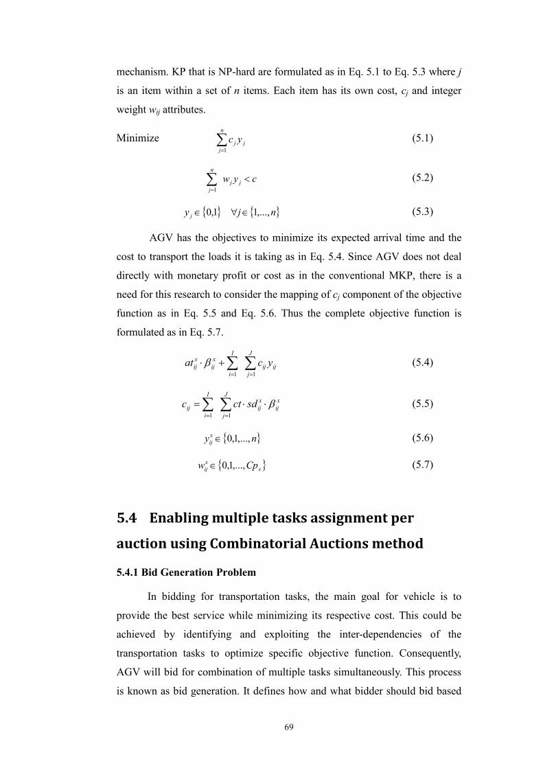
69
mechanism. KP that is NP-hard are formulated as in Eq. 5.1 to Eq. 5.3 where j
is an item within a set of n items. Each item has its own cost, cj and integer
weight wij attributes.
Minimize ∑=
n
jjj yc
1
(5.1)
cyw jj
n
j
<∑=1
(5.2)
{ }1,0∈jy { }nj ,...,1∈∀ (5.3)
AGV has the objectives to minimize its expected arrival time and the
cost to transport the loads it is taking as in Eq. 5.4. Since AGV does not deal
directly with monetary profit or cost as in the conventional MKP, there is a
need for this research to consider the mapping of cj component of the objective
function as in Eq. 5.5 and Eq. 5.6. Thus the complete objective function is
formulated as in Eq. 5.7.
∑∑==
+⋅J
jijij
I
i
xij
xij ycat
11
β (5.4)
∑∑==
⋅⋅=J
j
xij
xij
I
iij sdctc
11
β (5.5)
{ }ny xij ,...,1,0∈ (5.6)
{ }xxij Cpw ,...,1,0∈ (5.7)
5.4 Enabling multiple tasks assignment per
auction using Combinatorial Auctions method
5.4.1 Bid Generation Problem
In bidding for transportation tasks, the main goal for vehicle is to
provide the best service while minimizing its respective cost. This could be
achieved by identifying and exploiting the inter-dependencies of the
transportation tasks to optimize specific objective function. Consequently,
AGV will bid for combination of multiple tasks simultaneously. This process
is known as bid generation. It defines how and what bidder should bid based

70
on its objectives and constraints.
Each AGVA is equipped with this function and thus enables each of
them to plan their schedule and route. The function possesses components
from vehicle routing model and knapsack optimization model thus making it
as NP-hard problem. Discussion on how the model adapted knapsack problem
has been explained earlier [69]. Moreover, yxij refers to the quantity of a
homogenous transportation request in an indivisible package. This research
considers divisible package condition where each tasks does not necessarily
be transported in a prespecified package. As such, yxij = 1. BGP that is adopted
to determine the optimal task assignment is based on the integer programming
formulation as in the following:
Minimize ∑∑= =
⋅⋅+⋅I
i
J
j
xij
xij
xij
xij sdctat
1 1
ββ (5.8)
Subject to
xx
ijxij cttrat += (5.9)
( )[ ]∑∑= =
++++=I
i
J
j
xijijijij
xij
xijx twtvtdtrttact
1 1
)()( β (5.10)
1=xijβ (5.11)
xxm cpcc < (5.12)
0≥xmcc (5.13)
∑∈
⋅≤+S
Smx
xm
xm
xm cpclcc δ (5.14)
xn
xm
xm
xm ccclccce =+⇒= 1 (5.15)
0=−∑∑∈∈
L
Lno
xno
L
Lmn
xmn δδ (5.16)
0=− ∑∑∈∈
L
Lne
xne
L
Lmp
xmp
ij
ij
ij
ijδδ (5.17)
1=∑∈
L
Lmp
xmp
ij
ijδ (5.18)
1=∑∈
L
Lne
xne
ij
ijδ (5.19)

71
∑∈
=L
Lmn
xmn 1δ (5.20)
∑ ∑∈ ∈
≤+Lmn Lmn
xnm
xmn 1δδ (5.21)
x
ijxij
L
Lmn
J
Jj
I
Ii
x dsd δ∑∑∑∈∈∈
= (5.22)
1≥∑∈
xb
B
Bb
x
x
ξ (5.23)
AGVA has the objective to minimize both expected arrival time and its
respective transportation cost that complies to (5.8). Equation (5.9) calculates
the earliest predicted arrival time for the AGV could start the pickup. Eq.
(5.10) defines the expected completion time for assigned tasks. Eq. (5.11)
ensures only assigned tasks are taken into consideration when estimating
vehicle expected arrival time. Eq. (5.12) ensures that the number of tasks on-
board is less than the full capacity the vehicle can carry. Eq. (5.13) reflects
that loading capacity only takes non-negative values. Eq. (5.14) ensures
loading and unloading activities are conducted within the capacity limitation.
Eq. (5.15) is the binary decision variable represents the vehicle capacity.
AGV routing (Eq. 5.16 to Eq. 5.21) are based on conflict-free vehicle
routing with pickup and delivery principle [17], [70]. Eq. (5.16) represents
AGV routing continuity when visiting a particular machine. Any time when an
AGV travels to a station through its incoming lane, the constraint ensures that
the vehicle leaves through the outgoing lane. Eq. (5.17) obligates a vehicle to
deliver each picked up load to the final destination. Eqs. (5.18) and (5.19)
define the starting and destination nodes that an AGV needs to obligate. In
addition, Eq. (5.20) ensures that at any time, each AGV is located at a unique
position and Eq. (5.21) represents collision avoidance constraint. The AGV’s
bid generation model consist of a non-linear integer programming, which
demands long computation time. Eq. (5.22) calculates the resulted traveling
distance for the AGV. Eq. (5.23) necessitates the agent to involve in the
auction.

72
5.4.2 Winner Determination Problem
In an auction procedure, an auctioneer determines the winners—that is,
decides which bid is winning and which are losing based on the auctioneer’s
profitable gain. For single-task auction, such decision making is relatively
easy as it could be carried out by selecting the highest bid for each item
independently. However, WDP in combinatorial auctions is hard particularly it
deals with large instances with combinatorial behavior. Thus, there is an
important need to have an efficient computational system to address the
problem.
Let IJ represents the set of transportation tasks to be auctioned where
any AGVA can place a bid, bx (ij) > 0, for any combination IJij∈ . Number of
tasks in the bid define the upper limit of a bid length itself. Bid with the best
offer will be selected while others will be discarded. In this research bids
attributes are define as the following:
• the best bid for a package is define as bx(ij) = min bx(ij), Xx∈ ,
IJij∈ .
• if an agent does not bid for a task, bx(ij) = 0 is assigned for the
bidder.
Specific WDP function has been constructed as a mixed integer
programming model. Auctioneer utilizes the function to evaluate bids received
in an auction. The function should be able to single-out buyer with the best
bid hence awarding the contract/ good to the buyer. In this research, MA takes
the role as the auctioneer thus is equipped with the WDP module. The
function is designed to find the vehicle that could provide closest atx
compared to the teij.
Minimize ∑ ∑∈ ∈
⋅I
Ii
J
Jj
xb
xij ijad )(ξ (5.24)
Subject to
xijij
xij attead −= (5.25)
ijxijij tlatte ≤≤ (5.26)

73
jjjij mtdtrttl −+= (5.27)
mijij
mijijij tpatpte αα += (5.28)
( ) mijij
mijij
mij
mij
mij twtvtptpatpa αα ⋅+++≥ −−−− 1111 (5.29)
The MA’s objective function is to minimize the difference between
vehicle expected arrival time and earliest task pickup time as in (5.24). Eq.
(5.25) calculates the difference of earliest pickup start time and AGV expected
arrival time. Eq. (5.26) ensures that expected arrival time neither start before
the earliest task pickup time nor exceed the latest start time. Eq. (5.27) defines
the latest start time for operation-ij and Eq. (5.28) suggests the definition of
earliest start time. Eq. (5.29) ensures that machine operations should comply
with the precedence sequence for operations belong to the same job.
5.4.3 Design of Auction Coordination
Equipping the bidding agent with ability to analyze the tasks
interdependence means that it could judge the complementary attributes.
However, the mechanism still does not explicitly allow the agent to express
bidding substitutability. To do so, this research uses Exclusive OR (XOR) as
the bidding language so that bidders could indicate their interest in two
mutually exclusive bundles. The XOR auction rule used in this research is
based on these assumptions:
• Each and all of the tasks can be transported by any vehicle
within the system. Task is not required to be carried by a
specific AGV.
• Each and all of the tasks are divisible for transportation
purpose. No tasks need to be transported in specific group.
• The auction rule allows a bidder to express bidding
substitutability as long as the bidder fulfills all of the bidding
constraints
• A bidder may submit more than one bid package.
• At the end of an auction, a bidder can win at most one of its
bids.

74
The research introduces Auction Agent (AA) that is responsible to
implement the auction rules and coordinate the procedure. There is no specific
objective function need to be computed but in implementing the rules, the
agent is bound to:
• authenticates all bids submitted comply with XOR bidding rules
where:
Bx = {(b1) xor (b2) xor (b3)} and b1 = (<IJ, xijat >) (5.30)
• validates each task is awarded at most once (Eq. 5.31).
( ) mijij
mijij
mij
mij
mij twtvtptpatpa αα ⋅+++≥ −−−− 1111 (5.31)
• validates that the number of awards made do not exceed the
number of available tasks as in Eq. (5.32). This constraint is
important for conducting auction of multiple tasks.
m
xijm
J
Jj
I
Ii
IJIJ ≤⋅∑∑∈∈
β (5.32)
• Validate each AGV can only win at most one of its bids. The
constraint for a specific AGV complies with Eq. (5.33). This
constraint is a mandatory to fulfill the XOR constraint
implementation.
11 ≤⇒= ∑∈
xb
B
Bb
xb
x
x
ξξ (5.33)
While the first three rules are necessary to determine either stopping
criteria for the task assignment have been met, the forth rule: validation of
AGV winning requires specific protocol to be achieved.
In order to carry out the assignment validation, AA is equipped with
Validate Assignment function. The logic for the function is summarized as the
following while the conflict resolution protocol involved is illustrated in Fig
5.2:
If [ 1bξ ] <= 1
Then Propagate Message to AGVA1
Else If MA1_adxij < MA2_adx
ij
Then Request Revise Assignment to MA2

75
Propagate MA1_Assignment to AGVA1
Else If MA2_adxij < MA1_adx
ij
Then Request Revise Assignment to MA1
Propagate MA2_Assignment to AGVA1
Finish
Fig. 5.2. Sequence diagram for assignments conflict resolution.
5.5 Worked example
5.5.1 Problem Description
This section tests the effectiveness of the proposed auction-based task
assignment approach and compares them with other control methods.
Environment setting typically employed in a manufacturing plant is studied.
Eclipse IDE [47] has been used as the main tool for system
development. Simulation of the combinatorial auctions has been developed
based on Recursive Porous Agent Simulation Toolkit (Repast) platform [71].
Repast is an open-source agent-based simulation package that enables
MA_2 AA
MA_1 Assignment
MA_1
MA_2 Assignment
AGVA_1
Revise MA_2 AssignmentMA_1 Assignment
Validate Assignment
Revise MA_1 Assignment
Request M1_yxijRequest M2_yxij
Send M1_yxijSend M2_yxij

76
systemic study of complex system behaviors through controlled and replicable
computational experiments. Meanwhile, agent communication complies to
Agent Communication Language (ACL) standard provided by JADE. ILOG
CPLEX solver [49] was used to compute the functions for both the BGP and
WDP. Meanwhile, OptimJ [50] was used to integrate CPLEX solver into
Eclipse IDE. It is an extension of the Java with language support for writing
optimization models.
The shop floor configuration consists of a Flexible Manufacturing
System (FMS) as illustrated in Fig. 5.3. The path layout has been divided into
several path segments for route analysis purpose (numbers start with prefix
“A’, e.g: A1).
Fig. 5.3. Layout of an FMS.
The machine-to-machine distance for the shop floor is shown in Table
5.1 (in meter unit). Additionally, two job shop data set have been used
independently to evaluate the effectiveness of the proposed approach as the
following:
• Example 1.
• Example 2.

77
Table 5.1. Machine-to-machine distance chart.
Machine L/U M1 M2 M3 M4 M5 M6
L/U 0 160 240 320 560 480 400
M1 400 0 120 200 440 360 280
M2 480 600 0 120 360 280 360
M3 560 680 600 0 280 360 440
M4 320 440 360 280 0 120 200
M5 240 360 280 360 600 0 120
M6 160 280 360 440 680 600 0
System specification is as the following:
• The FMS consists of six CNC machines and two AGVs.
• Due time, dtj for each job is 35 minutes which also serves as the
maximum flow time for each job.
• Loading and unloading times are fixed at 0.5 min each.
• There are 6 job sets with each possessing six different operations
sequence, dedicated machine, M and processing time, PT. The
machine operations are given in M(PT) format, e.g.: M3(4)
means the operation by machine M3 takes 4 minutes to complete.
Details are given in Table 5.2 (Example 1) and Table 5.3
(Example 2).
• Vehicles constantly travel at 40 m/min.
• AGV does not need to return to Loading/ Unloading (L/U)
station in between transportation job.
• All resources are assumed to have 100% efficiency.
• Machines processing times are normally distributed with
standard deviation, σ = 0.5 minutes.
• Jobs arrival rate with mean, E = 20 minutes according to an
exponential distribution.
• First Come First Serve (FCFS) dispatching rule is employed in
managing L/U outgoing queue.

78
Table 5.2. Job set details (Example 1).
Job Set Operation sequence
1 2 3 4 5 6
1 M2 (1) M6 (3) M1 (6) M3 (7) M5 (3) M4 (6)
2 M1 (8) M2 (5) M4(10) M5(10) M6(10) M3 (4)
3 M2 (5) M3 (4) M5 (8) M6 (9) M1 (1) M4 (7)
4 M1 (5) M6 (5) M2 (5) M3 (3) M4 (8) M5 (9)
5 M2 (9) M1 (3) M4 (5) M5 (4) M6 (3) M3 (1)
6 M1 (3) M3 (3) M5 (9) M6(10) M4 (4) M2 (1)
Table 5.3. Job set details (Example 2).
Job Set Operation sequence
1 2 3 4 5 6
1 M3(1) M1(3) M2(6) M4(7) M6(3) M5(6)
2 M2(8) M3(5) M5(10) M6(10) M1(10) M4(4)
3 M3(5) M4(4) M6(8) M1(9) M2(1) M5(7)
4 M2(5) M1(5) M3(5) M4(3) M5(8) M6(9)
5 M3(9) M2(3) M5(5) M6(4) M1(3) M4(1)
6 M2(3) M4(3) M6(9) M1(10) M5(4) M3(1)
5.5.2 Experimental Work
To exemplify the solution methodology, this section implements the
combinatorial auction model into the specified FMS problem configuration.
Data communication involves during the auction are as the following:
• Data structure of the tasks announcement made by MA:
<IJ, pij, eij, tei, tlij>.
• Upon determining its suitability to transport the auctioned tasks,
AGVA will send set of bids attempting to acquire the tasks.
Bidding data submitted are:

79
Bx = {(b1) xor (b2) xor (bt)} where b1 = (<IJ, atxij >).
• Auctioneer will find the best offer and award the task to the
winner. The award data structure is <IJ, AGVx >.
Example 1
The first instance takes tasks assignment condition for 2 vehicles with
3-loading capacity each. Table 5.4 shows an example of six independent tasks
that need to be transported. The information in the table refers to the
information of the transportation request made by MA.
Table 5.4. List of transportation requests.
Operation ID Request ID pij eij teij tlij
ON6.2 L11 M3 M5 10:33 10:45
ON5.2 L12 M1 M4 10:32 10:40
ON0.1 L15 L/U M2 10:28 10:36
ON2.3 L16 M4 M5 10:43 10:54
ON5.1 L19 M2 M1 10:30 10:40
ON6.1 L20 M1 M3 10:35 10:45
ON3.4 L21 M6 M1 10:52 10:57
ON0.2 L24 L/U M1 10:55 11:02
ON4.3 L26 M2 M3 10:42 10:50
Upon starting the machine processing of operation-ij, MA computes
the expected finish time for the machine operation. The expected finish time
also serves as the earliest task pickup time, teij. Both teij and latest task pickup
time, tlij were computed based on Eq. 18 and Eq. 19. Both teij and tlij are the
timestamps and format of ‘hour:minute’ are used. Data on the pickup station,
pij and delivery station, eij could be extracted based on operation sequence
information in Table 5.2.
A standard naming convention is used as an identifier for all of the
operations. Operation is named based on its respective “job.operation
sequence” information format with “ON” prefix, e.g. the third operation of
Job 6 will be identified as ON6.3. Furthermore, in identifying transportation
requests, all of the requests are also labeled based on the chronological order.

80
Request names start with prefix “L”, e.g. L10.
Each bidder calculates the best transport combination it could offer
and submits the bid to the auctioneer. In this case each AGV would attempt to
minimize its traveling distance subject to a set of constraints. Shortest path for
AGV-x, dxij to transport load-ij from pickup node, pij to destination node, eij is
derived from the distance matrix.
Participant will then submit arbitrary number of bids as XOR bidding
rule is employed. Table 5.5 depicts partial bid specification generated and
subsequently submitted to auctioneers based on the auctioned tasks as in Table
5.4.
Table 5.5. Partial generated bid specification.
AGV Bid ID Bid Details (Request ID, atx)
AGV1 B1-1 (<L12,10.32>)
B1-2 (<L12,10.32>, <L16, 10.43>)
B1-3 (<L15, 10.28>, <L12,10.32>, <L20, 10.35>)
B1-4 (<L15, 10.28>, <L12,10.32>, <L20, 10.35>, <L26, 10.42>)
AGV2 B2-1 (<L19, 10.30>, <L11,10.34>)
B2-2 (<L19, 10.30>, <L11,10.34>, <L16, 10.42>)
B2-3
(<L19, 10.30>, <L11,10.34>, <L16, 10.42>, <L21, 10.51>,
<L24, 10.56>)
Transportation assignments are made based on the AGV that is capable
to provide the best pickup time compared to the earliest pickup start time. In
term of the AGV movement, a reasonably good vehicle routing could be
obtained based on the routing decision made. The awarded tasks are listed
Table 5.6.
Meanwhile, Fig. 5.4 depicts the traveling route for both vehicles and
their respective total traveling distances based on the awarded tasks (B1-4 and
B2-3 respectively). Supplementary to the route, Fig. 5.5 exhibits the travel
time window of both vehicles as well as the stops made for pickup and
delivery.

81
Table 5.6. Awarded tasks for each AGV.
AGV Awarded Tasks (respective atx sequence)
AGV1 L15, L12, L20, L26
(10.28, 10.32, 10.35, 10.42)
AGV2 L19, L11, L16, L21, L24
(10.30, 10.33, 10.43, 10.52, 10.56)
L/U
M2 M3 M4 M5 M6 L/U M1
M1 M2 M3 M4
2
2
21 1 1 1
1 1 1 1 31TD AGV2= 880 m
TD AGV1= 920 m L/U
M2 M3 M4 M5 M6 L/U M1
M1 M2 M3 M4
2
2
21 1 1 1
1 1 1 1 31TD AGV2= 880 m
TD AGV1= 920 m
Fig. 5.4. Vehicle routing based on the awarded tasks.
A1A2A3
A4A5
A6A7A8A9A10A11
10.30 10.35 10.40 10.45 10.50 10.55 11.0010.25
M3
M2
M4 M4
M5
M6L/U
L/U M1
M2
M3
Timeline
Arcs
AGV1 AGV2
M1
Legend
A1A2A3
A4A5
A6A7A8A9A10A11
10.30 10.35 10.40 10.45 10.50 10.55 11.0010.25
M3
M2
M4 M4
M5
M6L/U
L/U M1
M2
M3
Timeline
Arcs
AGV1 AGV2
M1
Legend
Fig. 5.5. Travel timeline of both vehicle.
Example 2
In addition to the first example, another case was also used to evaluate
the proposed method (the job set detail is given in Table 5.3). The instance for
list of the transportation requests for is provided in Table 5.7. AGV fleet of 4-
vehicle with 2-loading capacity were deployed for material transportation
purpose.

82
Table 5.7. List of transportation requests (Example 2)
Operation ID Request ID mpij mdij teij tlij
ON2.2 L112 M3 M5 4:10 4:15
ON3.5 L114 M2 M5 4:15 4:21
ON6.3 L115 M6 M1 4:15 4:26
ON5.5 L116 M1 M4 4:18 4:22
ON1.4 L117 M4 M6 4:18 4:26
ON0.5 L118 L/U M3 4:20 4:45
ON4.3 L120 M5 M3 4:25 4:38
Consequently, the tasks assignment for each of the vehicle is
summarized in Table 5.8.
Table 5.8. Awarded tasks for each AGV.
AGV Awarded Tasks (respective atx sequence)
AGV1 L112, L117 (4:10, 4:17)
AGV2 L115, L118 (4:15, 4:19)
AGV3 L116 (4:15)
AGV4 L114, L120 (4:15, 4:22)
The corresponding vehicle routing and the traveling timeline are
shown in Fig. 5.6 and Fig. 5.7. Based on Fig. 5.7, it is visible that there are
sufficient time gap among all of the AGVs when traveling along a path
segment.
M6
M3 M4 M5 M6
L/U M1 M3
1
TD AGV1= 480 m
11 1
1 1 1
M1 M4
11
M5M2
1
M3
11
TD AGV2= 480 m
TD AGV3= 440 m
TD AGV4= 640 m
1
1
M6
M3 M4 M5 M6
L/U M1 M3
1
TD AGV1= 480 m
11 1
1 1 1
M1 M4
11
M5M2
1
M3
1
M3
11
TD AGV2= 480 m
TD AGV3= 440 m
TD AGV4= 640 m
1
1
Fig. 5.6. Vehicle routing (Example 2)

83
AGV1
AGV2
AGV3
AGV4
4.15 4.20 4.25 4.30 4.35 4.404.10Timeline
A1
A2
A3
A4
A5
A6
A7
A8
A9
A10
A11
Arc
s
M3 M4
M5
M5
M6 L/UM1
M3
M2
A12
A13
M5
M3
M1
M4
Legend
Fig. 5.7. Travel timeline (Example 2)
5.6 Performance Measurement
This research decided to use the performance measurement of three
different aspects of the auction mechanism by using three performance
indicators (PI). The CA aspects and their respective PIs are as the following:
• System performance.
Throughput (STH) is selected as an indicator to measure the
performance of the system because it could reflects the system
efficiency as a consequence of implementing the proposed
method. Throughput is defined as the summation of the jobs
completed by the system.
• Bidders performance.
Percentage of fully loaded travel (FLT) is an important measure
to indicate the direct impact of the proposed method on the
bidders’ own operation. Percentage of fully loaded travel is
defined as the percentage of time duration the vehicles are fully
loaded in comparison to the entire operation time. Fully loaded
travel distance is computed by using Eq. (5.34) while the average
fully loaded travel is measured by Eq. (5.35).

84
∑∑∑∈ ∈ ∈
−=I
Ii
J
Jj
L
Lmnij
xijaxx tdCeloaded ))((1 β (5.34)
⋅=∑
∈ XtotalTimeloaded
FLT xX
Xx (5.35)
• Auctioneers performance.
In this case, auctioneers also act as the customers as winning
bidders will serve respective auctioneers. In order to measure the
impact of proposed method on the customer, average waiting
time is used as the indicator. In this case waiting time is defined
as the actual arrival time with regards to the earliest start time.
Total waiting time (in seconds) for each machine is defined as in
Eq. (5.36) and the average waiting time (PWT) is calculated as in
Eq. (5.37).
∑∑= =
−=I
i
J
j
mijijijm tetvawait
1 1
)( α (5.36)
=∑
= m
mM
m Jwait
PWT1 (5.37)
5.7 Result and analysis
Analysis has been conducted with the intention to demonstrate the
performance of auction-based task assignment technique for multi-load AGV.
Using Example 1, experiments have been carried out to investigate system
performance over a 24-hour production time. Experimental factors have been
varied as listed in Table 5.9 while the Design of Experiment (DOE) was based
on a full factorial design. Hence a total of 24 sets of simulation were
conducted.
Table 5.9. Experimental factors.
Factor Range (Value)
1 Loading capacity Low to high loading capacity (1, 3, 5, 7)
2 Fleet sizing Low to high number of vehicles (2, 4, 6, 8, 10, 12)

85
5.7.1 Performance Analysis
The resulted performances are as the following:
• STH analysis – Deployment of different number of vehicle
evoked different STH outcomes. The result shown in Fig. 5.8
ascertains that single-loading AGV is not capable to achieve the
throughput obtained by fleet of multi-load AGV. Additionally, the
deployment of vehicle with bigger loading capacity would directly
contribute to increase system throughput when compared to the
same number of vehicle with lower capacity. Vehicle with 5- and 7-
capacity reached maximum throughput with 6-AGV. Meanwhile 3-
capacity AGV only managed to reach the saturation points with 8-
AGV.
System Throughput (STH)
30
60
90
120
150
180
210
240
2 4 6 8 10 12No of Vehicle
Throughput
Cap-1 Cap-3Cap-5 Cap-7
Fig. 5.8. Comparison of STH
• PWT analysis – Fig. 5.9 depicts PWT comparison for all of the
capacity groups. We find that increasing the capacity would
result in lowering the pickup waiting time. The differences are
bigger when the NOV are smaller (2- and 4- AGV groups). It is
worth to mention that optimization function should not feature
maximizing the load quantity as an objective as it may directly
increase PWT.

86
Average Pickup Waiting Time (PWT)
0
50
100
150
200
250
2 4 6 8 10 12No of Vehicle
Time (second)
Cap-1 Cap-3
Cap-5 Cap-7
Fig. 5.9. Comparison of PWT
• FLT analysis – Fig. 5.10 illustrates the resulted capacity
utilization for the selected loading capacity. There are different
characteristics between single-load and multi-load categories.
Single-load AGV didn’t have huge impact on the characteristic
of FLT when number of vehicle is increased. On the contrary, the
FLT were reduced significantly when the NOV of multi-load
AGV were increased. In solving the specified FMS problem, 3-
capacity AGV proved to have the best performance in term of
capacity utilization particularly for NOV: 2-AGV and 4-AGV.
Percentage of Fully Loaded Travel (FLT)
0
20
40
60
80
2 4 6 8 10 12No of Vehicle
Percentage
Cap-1 Cap-3
Cap-5 Cap-7
Fig. 5.10. Comparison of FLT

87
Additionally, understanding the resultant of FLT would
provide fundamental knowledge on how vehicle capacities can
be utilized. For instance, if a warehouse or production plant
intents to expand their material handling capacity, they will be
able to take into account the utilization aspect.
Based on the analyzed results (in Fig. 5.8 to Fig. 5.10), it can be
summarized that utilizing multi-load AGV could reduce the NOV required in
achieving specific performance targets. Comparison on the achievement of
system performance between single-load (case: 8-AGV with 1-CAP) and
multi-load AGV (case: 2-AGV with 5-CAP) are as the following:
• Efficient energy utilization.
Analyzing the FLT achievement, single-load AGV resulted in FLT of
45% while multi-load AGV resulted in FLT of 52%. This shows that
utilization of multi-load AGV could result in better energy utilization by
obtaining higher percentage of fully loaded travel.
• Reduced NOV is required in achieving specific level of production
performance.
Single-load AGV is able to produce STH of 117 jobs. Alternatively,
utilizing multi-load AGV shows that multi-load AGV could produce
STH of 114 jobs; that is approximately the same level of STH. Looking
into performance of PWT, single-load AGV resulted in PWT of 112
seconds while multi-load AGV resulted in PWT of 116 seconds.
5.7.2 Sensitivity Analysis for Single Variable
In order to get the insight of how STH performance is affected by the
increment of CAP compared to the increment of NOV independently, the
analysis was extended by comparing the achievement of STH level for both
categories. Values for vehicle capacity and number of vehicle have been
varied. The corresponding STH are shown in Table 5.10.

88
Table 5.10. STH resulted from variation of design variable.
CAP Variation
2-Cap 4-Cap 6-Cap
NO
V
Var
iatio
n 2-AGV 51 94 129
4-AGV 108 - -
6-AGV 148 - -
Comparison between 2-AGV with 2- and 6-capacities demonstrates
that STH could be improved by 153%. Meanwhile, comparison between 2-
and 6-AGV with 2-capacity each resulted in throughput improvement of
190%. This proves that NOV has greater effect on STH compared to CAP.
The comparison is depicted in Fig. 5.11.
Fig. 5.11. Comparison of STH (design variable analysis)
5.7.3 Benchmark Study against Centralized Optimization Method
In order to determine the performance of the proposed method relative
to the conventional centralized optimization methods, we have conducted
benchmark study to compare the STH performance for case: 4-AGV with 3-
capacity. Fixed input has been used in order to provide equal requirement for
24
6 2
4
6
150
100
50
System Throughput (STH)
Number of Vehicle (NOV)
Vehicle Loading Capacity (CAP)
6-AGV 2-CAP
4-AGV2-CAP
2-AGV6-CAP
2-AGV4-CAP
2-AGV 2-CAP
3D Plot of STH vs CAP vs NOV
24
6 2
4
6
150
100
50
System Throughput (STH)
Number of Vehicle (NOV)
Vehicle Loading Capacity (CAP)
6-AGV 2-CAP
4-AGV2-CAP
2-AGV6-CAP
2-AGV4-CAP
2-AGV 2-CAP
3D Plot of STH vs CAP vs NOV

89
job arrival. Analysis for computational requirement considers the monitoring
period of 20 minutes involving the assignment of 12 transportation tasks.
In a conventional transportation task assignment approach, AGV
doesn’t need to bid for any transportation task. A centralized scheduler is
equipped with the necessary functions to allocate all of the tasks to the entire
fleet. For the Centralized Method, i) the optimization equations (Eq. 5.8 and
Eq 5.24) have been aggregated and ii) respective constraints (Eq. 5.9 to Eq.
5.23 and Eq. 5.25 to Eq. 5.29) been directly coded based on centralized
scheduler architecture. Mathematical model for Centralized Method is directly
coded and solved by using ILOG CPLEX software.
Yielded STH values and the computational requirements have been
analyzed as the following:
• STH comparison – Fig. 5.12 shows the STH achievement by both
Proposed and Centralized methods for different NOV. On average
the proposed method could achieved 82% of the STH produced by
the centralized system.
Fig. 5.12. Optimality Analysis (Comparison of STH)
• In term of the computational requirement, there are large gaps for the
time needed between both of the approaches as shown in Fig. 5.13.
The reason on why distributed approach needed far less time are due
STH: Proposed vs Centralized
0
20
40
60
80
100
120
140
160
4 6 8 10
Number of Vehicle
Throughput
Centralized_STH Proposed_STH

90
to the fact the optimization model has been decomposed into sub-
models where each agent solves the model that suits its own interest.
This enables parallel computing to be conducted within the system as
well as adheres to the principle of divide-and-conquer algorithm in
solving complex problem.
Computational Time
0100200300400500600700800
4 6 8 10No of Vehicle
Time (sec)
Centralized
Proposed
Fig. 5.13. Optimality Analysis (Comparison of computational time)
5.8 Summary
This study has proposed a combinatorial auction with XOR auction
rule approach to solve distributed task assignment problem for multiple
loading capacity AGV. Analysis has been carried out and performance
indicators shown that multi-load AGV could outperform single-load AGV
significantly. The chapter summarizes that:
• Even though centralized-approach may provide better solution, it
can’t provide it in a timely manner especially when the problem
size increases. This raises the feasibility issue particularly in
responding to various dynamic factors.
• There is a need to further investigate the interaction effects of both
design variables on multiple objective functions. This is important
particularly when large scale AGV system need to be designed. As
such, the chapter follows will discuss on the matter.

91
Chapter 6
Multi Objective Design
Procedure for AGV System
and Its Case Study
6.1 Introduction
This dissertation has presented the improved methods to establish an
efficient scheduling for autonomous AGV with multiple-loading capacity in
both Chapters 4 and 5. Another important perspective need to be studied when
considering the implementation of AGV system is the system design.
With regards to the operational design domain, among the important
aspect of AGV system design is vehicle requirement analysis. This research
refers vehicle requirement analysis as the process of defining the best
combination of design variables, which include the number of vehicle to
deliver specific amount of transportation requests and to obtain desired level
of performances.
Looking at the recent trend where AGVs have been deployed in
various other industrial sectors which include container terminals, hospital
and warehouses [72], [73], [74], providing an efficient system design method
is critical to ensure the actual implementations and investments will be
profitable.

92
This chapter focuses on addressing the issue by providing an effective
design tool to decide design parameter of MAS-based AGV system for multi-
objective problem. Two main approaches have been taken to establish the
simulation-approach of MAS-based AGV system design: i) development of
integrated simulation tool for MAS-based AGV system; ii) utilize RSM
method for optimizing design parameters’ values using dominance-based
multi-objective optimization approach.
6.2 Design Procedure of MAS-based AGV System
There are some stages needed in order to carry out the system design.
The stages utilized in this research include:
i) Model specification – acquisition of production system
specification.
ii) Model simulation – development of simulation model
based on the acquired specification.
iii) RSM analysis – analysis of simulation result to determine
best combination of design parameters.
RSM Analysis
Model Simulation
Model Specification
Production requirement
and specification
SIMUL8 Agent class
Step 1 Low-Order Polynomial Model
P-values
Significant curvature
No significant curvature
Step 2 Establish second-order polynomial model
εββββ ++++= ∑∑∑===
jiij
q
jjjj
q
jjj
q
jr xxxxy
1
2
110
Draw conclusion
Step 4 Optimize model
(Derringer and Suichdesirability method)
Step 3 Measure output responses
Desirability Function
Minimization
Maximization w
rr
rrr TU
yUd
−−
=w
rr
rrr TU
yUd
−−
=
w
rr
rr LT
Ld
−−
= ryw
rr
rr LT
Ld
−−
= ry
niniir xxxy ββββ ++++= ...21 210
Fig. 6.1.� Stages of AGV system design.

93
6.3 Configuration of the Proposed Design Tool
There are some components needed in order to carry out the system
design. The components are:
• Agent class is the collection of classes containing agents’ functions. It
is necessary to conduct agent-based AGV system design. Three types
of agent developed are AGV Agent, Machine Agent and Monitor and
Coordinate Agent.
• RSM Tool is necessary to carry out result analysis based on Response
Surface Method. RSM Tool uses input data from Simul8.
• Data Visualization Tool is necessary to provide graphical interactivity
of the RSM result. System designer will be able to use it in making
decision on the combination of design variables.
• Component Object Model (COM) is necessary to integrate agent object
into SIMUL8 program.
• Simul8 is necessary as the simulation tool.
• Windows as the computer Operating System used.
The proposed tool configuration is depicted in Fig. 6.2.
Fig. 6.2.� Tool configuration for AGV system design.
SIMUL8
Agent class (AGVA, MA, TA, AA)
RSM ToolData
Visualization Tool
Windows
COM
Simulation Data
RSM-Analyzed Data ICNP
SIMUL8
Agent class (AGVA, MA, TA, AA)
RSM ToolData
Visualization Tool
Windows
COM
Simulation Data
RSM-Analyzed Data ICNP

94
6.4 Case Study: Tire Manufacturing Factory
6.4.1 Material Transportation System
There are several factors need to be decided in implementing an AGV
system for tire manufacturing factory. Among the important perspectives is to
optimize the number of vehicle needed for material transportation purpose.
This is critical due to several reasons. Under-estimated number of vehicle
simply means insufficient medium of transportation that might affect the
schedule of the entire shop floor. Meanwhile, over-estimated number of
vehicle requires bigger capital investment will result to under-utilized vehicles
while increasing operational-related cost. This highlights the importance to
determine minimum number of vehicles required.
Basically, vehicle requirement can be determined by two main
approaches – analytical and simulation methods. Analytical methods employ
mathematical models and heuristic algorithms. Nevertheless, realistic material
transportation planning is a very complicated process and typically involves
various combinatorial problems. For instance, the decision on the best design
variables combination should consider various design parameters as well as
dynamic operation parameters which include randomness in job arrivals,
traffic congestion, alternate vehicle routing and failure. This makes the system
to have high nonlinearity where the impact of each factor and their
interactions are difficult to be analyzed and verified using analytical method
especially when large scale transportation system is considered. This justifies
the importance of applying simulation method to analyze vehicle requirements.
In this chapter, simulation approach is utilized to model a multi-load
AGV operation. Based on the result, the interactions of design parameters and
the resulted system performance were investigated. Based on the outcomes,
required minimum number of AGVs could be forecasted with respect to
specific performance targets. The study used tire manufacturing factory as a
target example.
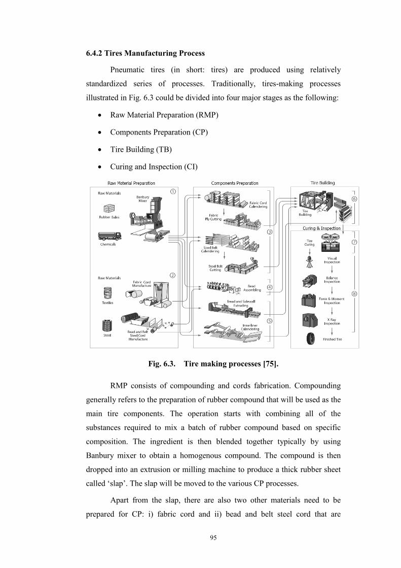
95
6.4.2 Tires Manufacturing Process
Pneumatic tires (in short: tires) are produced using relatively
standardized series of processes. Traditionally, tires-making processes
illustrated in Fig. 6.3 could be divided into four major stages as the following:
• Raw Material Preparation (RMP)
• Components Preparation (CP)
• Tire Building (TB)
• Curing and Inspection (CI)
Fig. 6.3.� Tire making processes [75].
RMP consists of compounding and cords fabrication. Compounding
generally refers to the preparation of rubber compound that will be used as the
main tire components. The operation starts with combining all of the
substances required to mix a batch of rubber compound based on specific
composition. The ingredient is then blended together typically by using
Banbury mixer to obtain a homogenous compound. The compound is then
dropped into an extrusion or milling machine to produce a thick rubber sheet
called ‘slap’. The slap will be moved to the various CP processes.
Apart from the slap, there are also two other materials need to be
prepared for CP: i) fabric cord and ii) bead and belt steel cord that are

96
prepared independently. CP provides the components required to build a tire.
Generally, the components could be classified based on their respective
needed production processes: calendaring, extrusion and bead building.
Components fall into three classes based on manufacturing process:
calendaring, extrusion, and bead building. Extrusions are used to produce tire
thread, sidewall profiles and inner liners. Calendaring process consists of
fabric calendar; steel belt calendar; and innerliner calendar that are needed to
produce body plies and belts (fabric and steel). Additionally, tire bead are also
assembled using Bead Building Machine.
All of the components produced are then transferred to a Tire Building
Machine (TBM). Conventional TB comprises of two-stage operation where
firstly- inner liner, body plies and sidewalls are wrapped around a drum. Then,
beads are attached to the assembly before sidewalls are pressed onto both
sides of the tire. In the second stage, the belt package, nylon cap and thread
are applied to complete the building of a ‘green tire’. It is then inflated and
ready to be cured.
Curing is an operation of applying high-temperature and high-pressure
to a green tire in a curing mold. By doing so, a series of chemical reactions
take place and these change the properties of the tire. The exterior shape of the
tire corresponds to the respective shape of the mold cavity used. A series of
tests and inspections are carried out to ensure the quality of the tire produced.
6.4.3 Simulation Model
The simulation model is based on tire manufacturing factory. Part of the
entire shop floor with process-based layout has been modeled with the
intention of studying the vehicle-based material transportation process. The
model possesses certain technical specifications and assumptions as the
following:
i) System specification
Plant layout used in the manufacturing system is based on
process layout. There are 19 process centers in the system where
each process has a set of machines as shown in Fig. 6.4. ‘IN’

97
refers to the station for incoming raw material while ‘OUT’
refers to the station for outgoing finished goods.
There are 5 job sets with each possessing specific number of
operation sequences. The detail of the job sets are described in
Table 6.1. In order to acquire stable data on the production flow,
the warm up period are fixed for 2 hours. Thus, data for analysis
purpose are only collected after the warm up period. Jobs arrival
rates of 80 jobs/ hour with mean, E follows a Poisson distribution.
Fig. 6.4.� Factory layout.
Table 6.1.� Job data set.
Job No
Volume Mix (%)
Machine sequence
(processing time in minutes)
1 25 P 1 (4) - P 2 (8) - P 3 (3) - P 14 (4) - P 17 (1) - P19 (12) - P 20 (1)
2 25 P 1 (4) - P 2 (8) - P 3 (3) - P 6 (3) - P 7 (1) - P 14 (4) - P 17 (1)- P 19 (12)- P 20 (1)
3 20 P 5 (2) - P 6 (3) - P 7 (1) - P 15 (5) - P 17 (1) - P 19 (15) - P 20 (1)
4 15 P 1 (4) - P 2 (8) - P 3 (3) - P 4 (4) – P 13 (3) - P 14 (4) - P 17 (1) - P 19 (15) - P 20 (1)
5 15 P 8 (3) - P 9 (5) - P 10 (1) - P 11 (8) - P 12 (4) - P 16 (6) - P 17 (1) - P 19 (22)- P 20 (1)

98
ii) Machine specification
Number of machines, m in the system is fixed. Machine’s
processing times are normally distributed with standard deviation,
σ = 0.5 minutes. In allocating specific operation to a machine
within a process group, rounded uniform distribution function
were used. Task loading and unloading times are fixed at 0.5
minute each. Finite numbers of input and output machine buffers
are used. First In First Out (FIFO) dispatching rule is employed
for the input and output buffers in prioritizing tasks in queue
waiting for a) processing on a machine and b) transportation.
iii) AGV specification
Multiple loading capacity AGVs are deployed for material
handling purpose. For standardization purpose, loading capacity
is based on the number of pallets regardless of the actual unit size
of a material. The number of AGVs, v in the system is known.
Vehicle’s velocity, velx are constant at 130 ft/min. The travel
paths connecting the processing machines are bidirectional. There
is no other material handling medium used. All machines and
AGVs are assumed to operate at 100% efficiency.
6.5 Proposed Method to Estimate Vehicle
Requirement
6.5.1 Discrete-Event Simulation as a Decision Support Tool
Discrete event simulation (DES) refers to simulation that employs
mathematical and logical models of a physical system to represent state
changes at precise points in simulated time [76]. Taking advantages of the
computing advancement, DES has been intensively developed for modeling,
simulating, and analyzing dynamic and complex systems. This is meant to
enable research on advanced industrial system to be conducted.
In this research, Simul8 simulation software [77] is used to model
material transportation operation within a manufacturing workplace. There are
several advantages of Simul8 software particularly in its ability to

99
accommodate mathematical and logical procedure with relative ease through
Visual Logic. Furthermore, it is also possible to integrate codes developed
using Visual Basic into Simul8 simulation framework. Based on the features,
we chose Simul8 as the tool to model proposed vehicle-based transportation
system in a tire manufacturing plant.
6.5.2 Response Surface Methodology
Response Surface Methodologies (RSM) is a combination of statistical
methods that are used to study the relationships between several explanatory
factors and the resulted response variables. RSM is a simple yet effective
method to optimize the responses when input factors are fixed, hence the
name response surface optimization. As such, it could be used to determine
optimal input factors when desired response variables are provided [79], [80].
RSM analysis starts with the approximation of a functional
relationship between explanatory variables and response variables. This is
carried out by a low-order polynomial modeling of the independent variables.
Simple linear regression model is assumed to sufficiently model the
relationship as in Eq. (6.1):
niniir xxxy ββββ ++++= ...
21 210 (6.1)
where yr are the output variables, βj are the unknown coefficients and xi are
coded units of the independent variables. The values for βs are determined
using the least square analysis method based on the simulation results.
Based on the results of variance analysis, if the developed models
show that obtained P-values are less than their respective significant levels,
then significant curvature of the relationship exists. This requires a second-
order polynomial model with two-factor interaction to be established
according to Eq. (6.2):
εββββ ++++= ∑∑∑===
jiij
q
jjjj
q
jjj
q
jr xxxxy
1
2
110 (6.2)
The output responses are measured for all of the simulation
experiments. Subsequently, the problem will be optimized based on Derringer
and Suich desirability method [81] where each response will be modeled
based on Eq. (6.3) for maximization and Eq. (6.4) for minimization functions.

100
Parameters needed to determine desirability function, dr are lower limit, Lr;
target value, Tr and upper limit, Ur.
w
rr
rr LT
Ld
−−
= ry
, rrr TyL ≤≤ (6.3)
w
rr
rrr TU
yUd
−−
=, rrr UyT ≤≤ (6.4)
The proposed flow for tuning of design variables is illustrated in Fig. 6.5.
Fig. 6.5.� Proposed flow for tuning of design variables.
6.6 Experimental Design
The experiments conducted were designed to achieve several
perspectives of the AGV operation. The experiment plans are classified based
on the following aspects:
• Design Variable (DV)
DV refers to the controllable input factors that are contemplated
during the development of an AGV system. The study starts with
experimenting two critical factors: i) number of vehicle (NOV) and
ii) AGV loading capacity (CAP).
Step 1 Low-Order Polynomial Model
P-values
Significant curvature
No significant curvature
Step 2 Establish second-order polynomial model
εββββ ++++= ∑∑∑===
jiij
q
jjjj
q
jjj
q
jr xxxxy
1
2
110
Draw conclusion
Step 4 Optimize model
(Derringer and Suichdesirability method)
Step 3 Measure output responses
Desirability Function
Minimization
Maximization w
rr
rrr TU
yUd
−−
=w
rr
rrr TU
yUd
−−
=
w
rr
rr LT
Ld
−−
= ryw
rr
rr LT
Ld
−−
= ry
niniir xxxy ββββ ++++= ...21 210

101
• Performance Variable (PV)
PV are uncontrollable factors resulted when a set of input factors
are utilized. Some of the important output factors used in this
research includes:
o System Throughput (STH) – STH is the amount of finished
goods produced by a system over a period of time. It is used to
measure the system-wide performance.
∑=
=I
iiFSTH
1
(6.5)
∑∑= =
=I
i
J
jiji foF
1 1
(6.6)
ijxijxijmijmijmijij ftfpfufo ,,,,, ** βθθ= (6.7)
o Mean Flow Time (MFT) – flow time, Fi refers to the time
duration required for a job to be completed. Parameters needed
to compute Fi include operation time, Oij; machine processing
time, tpij; transport time, ttij; loading/unloading time, tuij;
queuing time, tqij; job release time, Ri and total number of job
processed, n. MFT complies with Eqs. (6.8) to (6.11).
ijijijijij tqtutttpO +++= (6.8)
∑=
=n
iiji OC
1 (6.9)
iii RCF −= (6.10)
∑=
=n
iiF
nMFT
1
1 (6.11)
o Effective Total Distance Traveled (ETDT) - this research used
ETDT as an indicator to measure effectiveness of material
transportation. ETDT is defined as the ratio of total distance
traveled to STH produced. ETDT computation is defined in Eq.
(6.12). ETDT was selected because it could represent the
vehicle traveling efficiency with regards to the system
throughput.

102
STH
velpttaETDT
v
xxxx∑
== 1
)**(
(6.12)
Initial experiments are conducted based on a two-level full factorial
design. Details of the design variables are summarized in Table 6.2.
Table 6.2.� Input factors data.
Design
variable
Low level
(coded value: -1)
High level
(coded value: +1)
1 NOV 10 30
2 CAP 5 15
6.7 Simulation Analysis and Optimization
6.7.1 Simulation Analysis
Simulation has been carried out testing all of the combination of
experimental factors over 8-hour production time. Analysis had been carried
out with the intention to determine the performance of multi-load AGV. The
outcomes of the performance indicators are analyzed.
Deployment of different vehicle loading capacity resulted in different
STH outcomes. The result in Fig. 6.6 shows that deployment of vehicle with
different loading capacity resulted in significant throughput outcomes
particularly for smaller NOV category. On the other hand, the differences are
less when 20-AGVs are deployed. There is also a decreasing trend of
throughput specifically when the number of vehicles deployed is too high.

103
Comparison of STH
200
250
300
350
400
450
10 20 30No of Vehicle
Throughput
5-Cap10-Cap15-Cap
Fig. 6.6.� Comparison of STH.
In addition, we also analyze the ETDT data for each vehicle. Generally,
ETDT values drop when the numbers of AGVs are increased. Besides, there is
also significant improvement of ETDT particularly when AGVs with higher
loading capacity are utilized. The result depicts that AGV categories with 10-
and 15-capacities consistently have better ETDT compared to AGV with 5-
capacity. The result is depicted in Fig. 6.7.
Comparison of ETDT
700
900
1100
1300
1500
1700
1900
10 20 30No of Vehicle
Effective Total D
istance
Traveled (ratio)
5-Cap 10-Cap 15-Cap
Fig. 6.7.� Comparison of ETDT.
Moreover, MFT of the work-in-process materials has also been studied.
The result illustrated in Fig. 6.8 shows that generally, the MFT decreases
when the NOV increases up to a certain number of vehicles. Then, MFT starts
to increase back. This simply highlights the need to identify optimal design

104
variables when MTS is to be established. The result also shown that utilizing
vehicle with higher loading capacity could improve MFT outcome compared
to AGV with lower loading capacity.
Comparison of MFT
100
120
140
160
180
200
220
240
10 20 30No of Vehicle
Mean Flow Time
(minutes)
5-Cap 10-Cap 15-Cap
Fig. 6.8.� Comparison of MFT.
To support the discussion, we also carried out variance analysis
(ANOVA) on the simulation data obtained. The result is depicted in Table 6.3.
Based on the ANOVA conducted with a significance level of 5%, the main
effects and corresponding curvature were proved to be significant on various
PVs. This implies that the operational behavior cannot be explained by the
low-order model. Therefore, in order to optimize the problem’s solution,
second-order polynomial model is determined. Furthermore, the analysis
provided only consider single factor at a time.
Table 6.3.� ANOVA Result.
DP PV DF SS MS F P
NOV STH 2 31358 15679 16.03 0.004
NOV MFT 2 4529 2265 11.66 0.009
NOV ETDT 2 166117 83059 1.23 0.356
CAP STH 2 3692 1846 0.33 0.531
CAP MFT 2 1020 510 0.65 0.553
CAP ETDT 2 376349 188175 5.82 0.039
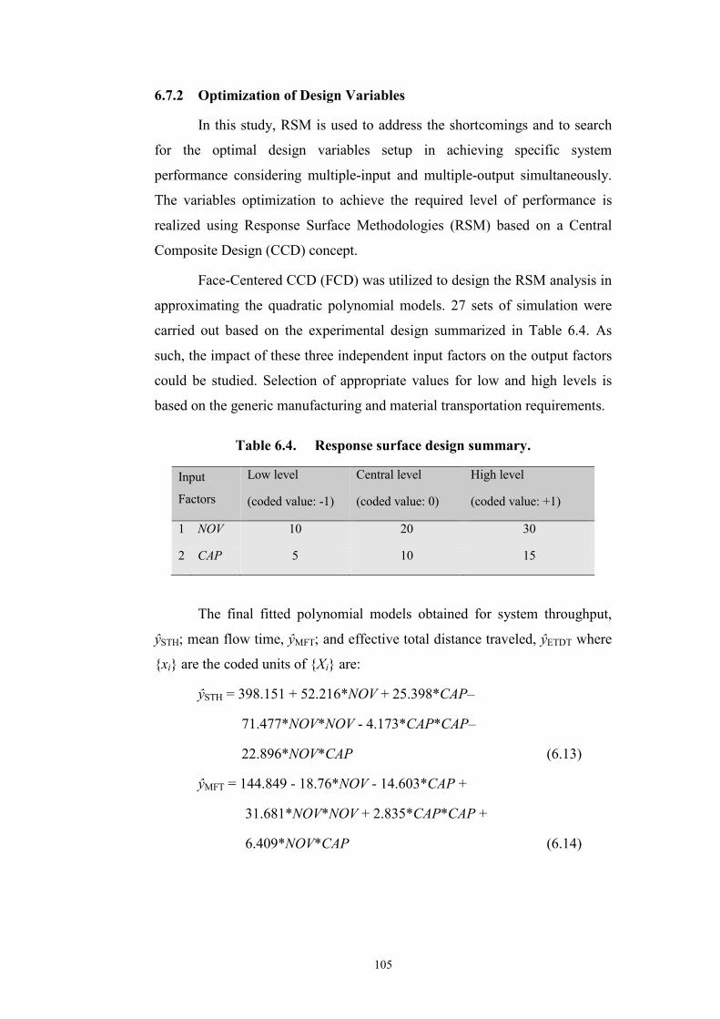
105
6.7.2 Optimization of Design Variables
In this study, RSM is used to address the shortcomings and to search
for the optimal design variables setup in achieving specific system
performance considering multiple-input and multiple-output simultaneously.
The variables optimization to achieve the required level of performance is
realized using Response Surface Methodologies (RSM) based on a Central
Composite Design (CCD) concept.
Face-Centered CCD (FCD) was utilized to design the RSM analysis in
approximating the quadratic polynomial models. 27 sets of simulation were
carried out based on the experimental design summarized in Table 6.4. As
such, the impact of these three independent input factors on the output factors
could be studied. Selection of appropriate values for low and high levels is
based on the generic manufacturing and material transportation requirements.
Table 6.4.� Response surface design summary.
Input
Factors
Low level
(coded value: -1)
Central level
(coded value: 0)
High level
(coded value: +1)
1 NOV 10 20 30
2 CAP 5 10 15
The final fitted polynomial models obtained for system throughput,
ŷSTH; mean flow time, ŷMFT; and effective total distance traveled, ŷETDT where
{xi} are the coded units of {Xi} are:
ŷSTH = 398.151 + 52.216*NOV + 25.398*CAP–
71.477*NOV*NOV - 4.173*CAP*CAP–
22.896*NOV*CAP (6.13)
ŷMFT = 144.849 - 18.76*NOV - 14.603*CAP +
31.681*NOV*NOV + 2.835*CAP*CAP +
6.409*NOV*CAP (6.14)

106
ŷETDT = 945.113 - 136.884*NOV - 149.564*CAP +
219.802*NOV*NOV + 104.390*CAP*CAP +
71.453*NOV*CAP (6.15)
Analysis was extended in order to determine optimal combination of
DPs for the case problem. Derringer - Suich desirability approach was utilized
to explore input variable settings with a higher composite desirability.
Basically, each response is given an individual desirability function, di from
which are used to identify each response independently.
The respective values are based on the simulation results obtained.
Based on Eq. (6.3) and Eq. (6.4), the desirability functions for the output
responses are governed by Eq. (6.16) to Eq. (6.18) respectively:
STHw
STHd
−=
506217ySTH
, 506217 ≤≤ STHy (6.16)
MFTwMFT
MFT
yd
−=
115218
, 218115 ≤≤ MFTy (6.17)
ETDTwETDT
ETDTy
d
−=
7161634
, 1634918 ≤≤ ETDTy (6.18)
This research utilizes equal weightage of desirability functions, i.e.:
wSTH = wMFT = wETDT. The RSM analysis has been conducted using Minitab 15
Statistical Software [82]. Independent results for each of the performance
objective are shown in Fig. 6.9.
Resulted achievements of the objective functions are summarized
using 3-dimensional response surface chart illustrated in Fig. 6.10. This will
enable system designer to evaluate all of the candidate solutions in providing
the best combination of DPs for the system.
Additionally, the information on optimum DP values and the
corresponding predicted responses are listed in Table 6.5.

107
Fig. 6.9.� Result for each of the objective.
Fig. 6.10.� Response surface chart for AGV system design.
ETDT (ratio)
MFT (mins)

108
Table 6.5.� Response surface predicted result.
Proposed Inputs Predicted Responses
NOV 22 STH 508
CAP 14 MFT 110
ETDT 807
6.8 Summary
The chapter has successfully achieved its aims to optimize design
variables for vehicle-based material transportation problem in a tire-
manufacturing factory. Optimization has been conducted using combined
DES and RSM methods. Based on specified objectives and performance
levels, optimal values for design parameters could be obtained thus enabling
management to make informed decision.

109
Chapter 7
Conclusions and Future
Works
7.1 Conclusions The dissertation focuses on the development of an efficient scheduling
method for dynamic and autonomous AGV system based on MAS
architecture. Three critical problems as the following have been addressed:
i) Existing task sharing protocol does not envisage dynamism of
AGV operation thus leads to system underperformance.
ii) Existing scheduling methods on distributed-controlled AGV does
not provide appropriate solution for AGV with multiple-loading
capacity.
iii) The research models for AGV system design either do not
contemplate multiple-loading capacity factor or were based on
simplified working example for evaluation purpose. In order to
design a realistic AGV system, it is necessary to analyse a realistic
production environment.
Therefore, this dissertation proposed appropriate methods to solve
abovementioned problems categorically. The work outcomes can be
summarized as the following:

110
i) Specific protocol has been developed to manage two important
dynamic factors in AGVs operation which are dynamic status of
vehicle availability and the positioning advantage of certain
vehicles in handling a particular transportation request have been
exploited. ICNP mechanism has been proposed that enable task to
be re-assigned to a later bidder (AGVA) with better solution.
Furthermore, a location-aware algorithm was introduced to
distinguish vehicles within strategic distance to the pickup station.
In order to demonstrate the effectiveness of the proposed
protocol, experiments have been carried out where three important
transportation–related performance indicators were measured.
Different values for NOV are used and the result proves that the
ICNP outperformed SCNP method significantly where STH is
improved by 25%, PLT of 80% is achievable and AWT is
consistently reduced (81% decrease for 4-AGV case) could be
achieved by applying ICNP method compared to SCNP.
ii) A market-based method is adapted to schedule autonomous AGV
fleet consisting of vehicle with multiple-loading capacity. This
successfully overcomes the weakness of conventional auction
where only one job is allocated in a single auction. Meanwhile,
combinatorial auctions (CA) mechanism was used in order to
realize the task assignment protocol for the multi-load AGV
scheduling. The functions have been divided into three
components: bid generation, winner determination and auction
coordination. Mixed Integer Programming (MIP) is used to obtain
the solution. Meanwhile, Knapsack problem model was utilized to
formalize AGV’s capacity utilization.
Comparison on the achievement of system performance
between single-load (case: 8-AGV with 1-CAP) and multi-load
AGV (case: 2-AGV with 5-CAP) are as the following:
o Efficient energy utilization.
Analyzing the FLT achievement, single-load AGV resulted
in FLT of 45% while multi-load AGV resulted in FLT of

111
52%. This shows that utilization of multi-load AGV could
result in better energy utilization by obtaining higher
percentage of fully loaded travel.
o Reduced NOV required in achieving specific level of
production performance.
Single-load AGV is able to produce STH of 117 jobs.
Alternatively, utilizing multi-load AGV shows that multi-
load AGV could produce STH of 114 jobs; that is
approximately the same level of STH. Looking into
performance of PWT, single-load AGV resulted in PWT of
112 seconds while multi-load AGV resulted in PWT of 116
seconds.
Furthermore, the proposed method could reduce
computational effort by 90% relative to the centralized-approach
optimization.
iii) Combination of DES and RSM has been utilized to estimate the
appropriate number of vehicle needed to achieve specific
performance objectives. Vehicle requirement estimation is needed
to design an AGV system. The problem is defined as to determine
the best combination of AGV design variables (number of vehicle
and its loading capacity) in delivering transportation requests to
achieve desired target performance. The experiment case is based
on data of a tire manufacturing factory involving multiple
transportation objectives: i) mean flow time; ii) average pickup
waiting time; and iii) total distance travelled.
Discrete Event Simulation and Response Surface
Methodology (RSM) were employed to obtain the best
combination of design variables. The result shows that determining
proper variables combination is critical to acquire desired level of
performance particularly when plural conflicting objectives were
involved. Deliverable of this chapter includes the fleet-sizing
decision support mechanism to design an AGV system. With
regards to the case study, the numerical results are:

112
o Proposed DP: 22-AGV with 14-CAP
o Predicted Responses: STH: 508 jobs (average: 4115
transportation tasks); MFT: 110 minutes; ETDT:807 (average:
5.7 kilometers/ AGV)
7.2 Future Works
There are a number of interesting topics that could be studied in
extending this research. In ensuring research continuity, two topics within
HMS domain have been selected as possible future research directions:
• Autonomous MTS holon considering special feature
In order to guarantee that an autonomous MTS could operate
efficiently, there are several special features need to be addressed
particularly for real-time applications. Those include:
o Breakdown and dynamic fault-tolerant strategy.
o Group of vehicles with heterogeneous vehicle attributes and
capabilities.
o AGV scalability accommodating incoming or outgoing vehicle.
o Autonomous MTS with multiple types of equipment.
• Integration of HMS-inspired AGV-centric manufacturing system.
We have demonstrated the importance of having an efficient an MTS
in improving the performance of a manufacturing system. As such, we
deem that it is a worthy effort to integrate the functional components
of an HMS with MTS as the central point. Therefore AGV-centric
HMS may provide an interesting future research direction.

113
List of References
[1] Hendrik Van Brussel. “Reference architecture for holonic manufacturing systems: PROSA”. Computers in Industry. Volume 37, Issue 3, Pages 255–274. 1998.
[2] Paulo Leitao. “An agile and adaptive holonic architecture for manufacturing control”. PhD Thesis. Department of Electrotechnical Engineering, Polytechnic Institute of Braganca. 2004.
[3] Morten Linda and Olivier Roulet-Dubonneta. “Holonic shop-floor application for handling, feeding and transportation of workpieces”. International Journal of Production Research, Volume 49, Issue 5, pages 1441-1454. 2011.
[4] F. Ounnar and P. Pujo. “Pull control for job shop: holonic manufacturing system approach using multicriteria decision-making”. Journal of Intelligent Manufacturing, Volume 23, Number 1, Pages 141-153. 2012.
[5] Olivier Roulet-Dubonnet et. al. “Development of a Holonic Free-Roaming AGV System for Part Manufacturing. Lecture Notes in Computer Science, Volume 5696, pp. 215-224. 2009.
[6] Julia Collins and Ryan Quinlan. “The impact of bidding aggregation levels on truckload rates”. Master's Thesis. Master of Engineering in Logistics. Engineering Systems Division. Massachusetts Institute of Technology. 2010.
[7] Yue Jin and Ana Muriel. “Single-warehouse multi-retailer inventory systems with full truckload shipments”. Naval Research Logistics (NRL). Volume 56, Issue 5, pages 450–464. 2009.
[8] Pranav J. Deshpande, Ali Yalcin, José Zayas-Castro and Luis E. Herrera. “Simulating less-than-truckload terminal operations”, Benchmarking: An International Journal, Vol. 14 Iss: 1, pp.92 - 101. 2007.
[9] Hiroyuki Yoshikawa. “Manufacturing and the 21st century — Intelligent manufacturing systems and the renaissance of the manufacturing industry”. Technological Forecasting and Social Change, Volume 49, Issue 2, Pages 195–213. 1995.
[10] Adriana Giret & Vicente Botti. “Engineering Holonic Manufacturing Systems”. Computers in Industry, Volume 60, Issue 6, Pages 428–440. 2009.

114
[11] Mikell P. Groover. “Automation, Production Systems, and Computer-Integrated Manufacturing”. 3rd Edition. Prentice Hall Press Upper Saddle River, NJ, USA. 2008.
[12] When is an AGV System the Best Solution? Available: http://www.hksystems.com/agv/why-agv.cfm?m=2&s=6 Retrieved: July 10, 2009.
[13] Mailmobile Automatic Mail Delivery AGVs. Available: http://www.egeminusa.com/pages/agvs/agvs_mailmobile.html Retrieved: August 31, 2010.
[14] Automated Container Transport- Proven Technology from Gottwald. Available: http://www.gottwald.com/gottwald/export/gottwaldsite/de/news/pdf/AGV_Prospekt_uk.pdf Retrieved: August 31, 2010.
[15] Iris F.A. Vis: “Survey of research in the design and control of automated guided vehicle systems”. European Journal of Operational Research, Volume 170 Issue 3 pp. 677–709. 2006.
[16] Tuan Le-Anh and M.B.M. De Koster. “A review of design and control of automated guided vehicle systems”. European Journal of Operational Research, Volume 171, Issue 1, pp. 1–23. 2006.
[17] Tamer F. Abdelmaguid and Ashraf O. Nassef. “A constructive heuristic for the integrated scheduling of machines and multiple-load material handling equipment in job shops”. Int J Adv Manuf Technol. Volume 46, Numbers 9-12, pp. 1239-1251. 2010.
[18] M. S. Akturk and H. Yilmaz. “Scheduling of Automated Guided Vehicles in a Decision Making Hierarchy”. International Journal of Production Research. Volume 34, Issue 2, pp. 577-591. 1996.
[19] Gang Dong, Jiafu Tang, Kin Keung Lai and Yuan Kong. “An exact algorithm for vehicle routing and scheduling problem of free pickup and delivery service in flight ticket sales companies based on set-partitioning model”. Journal of Intelligent Manufacturing, Volume 22, Number 5, Pages 789-799. 2011.
[20] Arif Imran, Said Salhi and Niaz A. Wassan. “A variable neighborhood-based heuristic for the heterogeneous fleet vehicle routing problem”. European Journal of Operational Research. Volume 197, Issue 2 Pages 509–518. 2009.
[21] W. K. Chang and J. M. A. Tanchoco. “Conflict-free shortest-time bidirectional AGV routeing”. International Journal of Production Research. Volume 29, Issue 12, pages 2377-2391. 1991.
[22] S. P. Singh and M. K. Tiwari. “Intelligent agent framework to determine the optimal conflict-free path for an automated guided vehicles system”. International Journal of Production Research. Volume 40, Issue 16, pp. 4195-4223. 2002.
[23] Pooya Farahvash and Thomas O. Boucher. “A multi-agent architecture for control of AGV systems”. International Journal of Robotics and Computer-Integrated Manufacturing. Vol. 20(6). Pages 473-483. 2004

115
[24] Michael Wooldridge. “An Introduction to MultiAgent Systems”. John Wiley & Sons Ltd. 2002.
[25] M.R. Genesereth and S.P. Ketchpel. “Software agents”. Communications of the ACM Volume 37 (7), pp. 48–53. 1994.
[26] A. Moukas and G. Zacharia, “Evolving a multi-agent information filtering solution in amalthaea”. In Proceedings of First International Conference on Autonomous Agents. ACM. pp. 394–403. 1997.
[27] Moses Ekpenyong and Eno-Abasi Urua. “Agent-based framework for intelligent natural language interface”. Telecommunication Systems. 2011. DOI: 10.1007/s11235-011-9620-3.
[28] R.G. Smith. “The Contract Net Protocol: High-Level Communication and Control in a Distributed Problem Solver”. IEEE Transactions on Computers, Vol. C-29 Issue 12 pp. 1104 - 1113. 1980.
[29] IEEE Foundation for Intelligent Physical Agents (FIPA). Available: http://www.fipa.org/ Retrieved: May 16, 2010.
[30] Foundation for Intelligent Physical Agents: “FIPA Contract Net Interaction Protocol Specification - Document number: SC00029H”, FIPA-Standard. Available from: URL: http://www.fipa.org/specs/ fipa00029/ [Accessed: April 20, 2010]
[31] D. P. Bertsekas: “Network Optimization: Continuous and Discrete Models (Optimization, Computation, and Control)”. Athena Scientific (1998)
[32] Agent Platform Special Interest Group. Available: http://agent.omg.org/ Retrieved: May 16, 2010.
[33] AgenLink. Available: http://www.agentlink.org/index.php Retrieved: Feb 2, 2011.
[34] P. Cramton, Y. Shoham and R. Steinberg (ed.). “Combinatorial Auctions”. The MIT Press. Ed. 1, Vol. 1. 2010.
[35] S. D. Vries and R. V. Vohra. “Combinatorial Auctions: A Survey”. INFORMS Journal on Computing, Vol. 15, No. 3, pp. 284-309. 2003.
[36] S. Pal, S.R. Kundu, M. Chatterjee and S.K. Das. “Combinatorial Reverse Auction based Scheduling in Multi-Rate Wireless Systems”. IEEE Transactions on Computers, Vol. 56 (10), pp. 1329- 1341. 2007.
[37] Ravi Bapna, Sanjukta Das, Robert Garfinkel and Jan Stallaert. “A Market Design for Grid Computing”. INFORMS Journal on Computing, Vol. 20 Issue 1, pp. 100 – 111. 2008.
[38] Djamila Ouelhadj and Sanja Petrovic. “A survey of dynamic scheduling in manufacturing systems”. Journal of Scheduling. Volume 12, Number 4, pp. 417-431. 2009.
[39] N. R. Jennings and M. Wooldridge. “Application of intelligent agents”. In: Jennings NR, Wooldridge MJ (eds) Agent technology foundation, applications and markets. Springer. pp 3–28. 1998.

116
[40] B. I. Kim, R. J. Graves, S. S. Heragu and A. S. Onge. “Intelligent agent modeling of an industrial warehousing problem”, IIE Transaction, Vol. 34 (7), pp. 601–612. 2002.
[41] S. C. Srivastava, A. K. Choudhary, S. Kumar and M. K. Tiwari. “Development of an intelligent agent-based AGV controller for a flexible manufacturing system”. International Journal of Advanced Manufacturing Technology Vol. 36, pp. 780–797. 2007.
[42] M. Nandula and S. P. Dutta. “Performance evaluation of an auction-based manufacturing system using colored Petri nets”. International Journal of Production Research Vol. 38 (10), pp. 2155–71. 2000.
[43] T. T. Tai and T. O. Boucher. “An Architecture for Scheduling and Control in Flexible Manufacturing Systems Using Distributed Objects”. IEEE Transactions on Robotics and Automation Vol. 18 (4), pp. 452 – 462. 2002.
[44] S. S. Heragu, R. J. Graves, B. I Kim and A. S. Onge. “Intelligent agent based framework for manufacturing systems control”. IEEE Transaction of System, Man, Cybernetics; Part A, Vol. 32 (5), pp. 560–73. 2002.
[45] M. Mes, M. van der Heijden and A. van Harten. “Comparison of agent-based scheduling to look-ahead heuristics for real-time transportation problems”. European Journal of Operational Research, Vol. 181 (1), pp. 59–75. 2007.
[46] B. S. P. Reddy and C. S. P. Rao. “A hybrid multi-objective GA for simultaneous scheduling of machines and AGVs in FMS”. Int. Journal of Advanced Manufacturing Technology, Vol. 31 (5-6), pp. 602-613. 2006.
[47] Eclipse SDK. Available: http://www.eclipse.org/. Retrieved: May 16, 2010
[48] F. Bellifemine, G.. Caire, A. Poggi and G. Rimassa. “JADE White Paper”. Telecom Italia Lab. 2003.
[49] Srinivas, M. K. Tiwari and V. Allada. “Solving the machine-loading problem in a flexible manufacturing system using a combinatorial auction-based approach”. International Journal of Production Research. Vol. 42 Part 9, pages 1879-1894, 2004.
[50] T. Kaihara, N. Fujii, S. Toide, H. Ishibashi and T. Nakano. “Optimization Method using Combinatorial Auction for Production Scheduling with Batch Processing”. Journal of Advanced Mechanical Design, Systems, and Manufacturing, Vol. 4, No. 3, pp.588-596, 2010
[51] M.Nanjanath, and M. Gini. “Dynamic Task Allocation for Robots via Auctions”. Proc. IEEE International Conference on Robotics and Automation (ICRA), pp. 2781 – 2786. 2006.
[52] Y.C Ho and S. H. Chien. “A simulation study on the performance of task-determination rules and delivery-dispatching rules for multiple-load AGVs”. International Journal of Production Research, Vol. 44 No. 20, pp. 4193 - 4222, 2006.

117
[53] Y. C Ho and H. C. Liu. “A simulation study on the performance of pickup-dispatching rules for multiple-load AGVs”. Computers & Industrial Engineering, Vol. 51, Issue 3, pp. 445-463. 2006.
[54] D. B. Kim and H. Hwang. “A Dispatching Algorithm for Multiple-Load AGVs Using a Fuzzy Decision-Making Method in a Job Shop”. Engineering Optimization, Vol. 33: 5, pp. 523 – 547. 2001.
[55] J. Abrache, T. G. Crainic, M. Gendreau and M. Rekik. “Combinatorial Auctions”. Annals of Operations Research. Vol. 153, No. 1, pp. 131-164. Springer, 2007.
[56] K. Tsubouchi, H. Yamato and K. Hiekata: “Innovative on-demand bus system in Japan”, IET Intelligent Transport Systems. Vol. 4 Issue 4, pp. 270 – 279. 2010.
[57] K. Kawamura and N. Mukai. “Optimization of Transport Plan for On-Demand Bus System Using Electrical Vehicles”. Proceedings of International Conference on Knowledge-Based and Intelligent Information & Engineering Systems (KES), Part 2, pp. 656-663. 2009.
[58] Cantillon and M. Pesendorfer: “Chapter 22: Auctioning Bus Routes: The London Experience”. in Ausubel, Cramton and Steinberg, Combinatorial Auctions, MIT Press. 2006.
[59] Jean-François Cordeau and Gilbert Laporte. “The dial-a-ride problem: models and algorithms”. Annals of Operations Research, Vol. 153 Issue 1. Page 29 – 46. 2007.
[60] Sophie N. Parragh, Karl F. Doerner and Richard F. Hartl. “Variable neighborhood search for the dial-a-ride problem”, Computers & Operations Research, Vol. 37 Issue 6, pp. 1129-1138. 2010.
[61] Lubomír Bakulea. “Decentralized control: An overview”. Annual Reviews in Control, Vol. 32, Issue 1, pp. 87-98. 2008.
[62] Paulo Leitão. “Agent-based distributed manufacturing control: A state-of-the-art survey”, Engineering Applications of Artificial Intelligence, Vol. 22, Issue 7, pp. 979-991. 2009.
[63] Martijn Mes, Matthieu van der Heijden and Jos van Hillegersberg. “Design choices for agent-based control of AGVs in the dough making process”. Decision Support Systems, Vol. 44 Issue 4. pp 983-999. 2008.
[64] Wallace A. “Application of AI to AGV control-agent control of AGVs”. Int. Journal of Production Research, Vol. 39 (4), pp. 709–726. 2001.
[65] Ying-Chin Ho and Hao-Cheng Liu. “A simulation study on the performance of pickup-dispatching rules for multiple-load AGVs”. Computers & Industrial Engineering, Vol 51, Issue 3, pp. 445-463. 2006.
[66] Han-Lim Choi, L. Brunet, and J.P How. “Consensus-Based Decentralized Auctions for Robust Task Allocation”. IEEE Transactions on Robotics, Vol. 25 Issue 4, pp. 912 – 926. 2009.

118
[67] Muhammad Hafidz Fazli Md Fauadi, Li Wan-Ling and Tomohiro Murata. “Combinatorial Auction Method for Decentralized Task Assignment of Multiple-Loading Capacity AGV based on Intelligent Agent Architecture”. Proceedings of IEEE Int. Conference on Innovations in Bio-Inspired Computing & Applications (IBICA 2011), Dec 16-18th 2011, China. 2011.
[68] Ayoub Insa Correa, Andre Langevin and Louis-Martin Rousseau. “Scheduling and routing of automated guided vehicles: A hybrid approach”. Computers & Operations Research Volume 34, Issue 6, pp. 1688–1707. 2007.
[69] Recursive Porous Agent Simulation Toolkit (Repast): Internet: http://repast.sourceforge.net/, [March 20, 2011].
[70] IBM ILOG CPLEX Optimization Studio: Internet: http://www-01.ibm.com/software/integration/optimization/cplex-optimization-studio/, [August 1, 2011].
[71] OptimJ. Internet: http://www.ateji.com/optimj/, [May 16, 2011]. [72] Chang Yang, Yong Choi and Tae Ha. “Simulation-based
performance evaluation of transport vehicles at container terminals”. OR SPECTRUM, Vol. 26 No 2 pp. 149-170. 2004.
[73] Automatic Guided Vehicles for the Hospital. Available: http://www.jbtc-agv.com/en/solutions/industries/hospital [Accessed: November 20, 2011]
[74] Min Zhang, Rajan Batta and Rakesh Nagi. “Modeling of Workflow Congestion and Optimization of Flow Routing in a Manufacturing/Warehouse Facility”. Management Science Journal, Vol. 55 No. 2 pp. 267-280. 2009.
[75] How a Tire is Made. Available: http://www.maxxis.com/ AutomobileLight-Truck/How-a-Tire-is-Made.aspx [Accessed: Nov. 10, 2011]
[76] Nance, Richard E. A. “History of Discrete Event Simulation Programming Languages”. Technical Report TR-93-21, Virginia Polytechnic Institute and State University. 1993. Available: http://eprints.cs.vt.edu/archive/00000363/ [Accessed: Dec 2, 2011]
[77] SIMUL8 simulation software. Available: http://www.simul8.com/ [78] Nuran Bradley. “The Response Surface Methodology”. Master thesis.
Indiana University of South Bend. 2007. [79] Tauseef Aized. “Modelling and performance maximization of an
integrated automated guided vehicle system using coloured Petri net and response surface methods”. Computers & Industrial Engineering, Vol. 57 (3) pp. 822-831. 2009.
[80] Derringer, G.C. and Suich, R. “Simultaneous optimization of several response variables”. Journal of Quality Technology, Vol. 12 (4), pp. 214–219. 1980.
[81] Minitab Statistical Software. Available: http://www.minitab.com/ [Accessed: January 16, 2012]

119
List of Publications
Referred journals
• Muhammad Hafidz Fazli bin Md Fauadi, Saifudin Hafiz Yahaya and
Tomohiro Murata. “Intelligent Combinatorial Auction of
Decentralized Task Assignment for AGV with Multiple Loading
Capacity”. IEEJ Transactions on Electrical and Electronic Engineering,
Vol.8, No.4, 2013. Accepted.
• Muhammad Hafidz Fazli bin Md Fauadi, Hao Wen Lin and Tomohiro
Murata. “Dynamic Task Assignment of Autonomous Distributed AGV
in an Intelligent FMS Environment”. IEEJ Transactions on Electronics,
Information and Systems, Vol.132, No.5, Pp. 697-705. 2012.
Referred international conferences
• Muhammad Hafidz Fazli bin Md Fauadi, Wan-Ling Li, Tomohiro
Murata and.Anton Satria Prabuwono. “Vehicle Requirement Analysis
of an AGV System using Discrete-Event Simulation and Data
Envelopment Analysis”. Proceedings of IEEE International
Conference on Computing Technology and Information Management
(ICCM 2012). Pp. 819-823. Seoul, Korea. April 24-26, 2012.
• Muhammad Hafidz Fazli bin Md Fauadi, Wan-Ling Li and Tomohiro
Murata. “Combinatorial Auction Method for Decentralized Task
Assignment of Multiple-Loading Capacity AGV based on Intelligent
Agent Architecture”. Proceedings of IEEE International Conference
on Innovations in Bio-inspired Computing and Applications (IBICA
2011). Pp. 207 – 211. Shenzhen, December 16-18, 2011.
120
• Wan-Ling Li, Muhammad Hafidz Fazli bin Md Fauadi and Tomohiro
Murata. “Performance Optimization of Reconfigurable Manufacturing
Cell with Flexible Routing Capacity in Presence of Unreliable
Machines”. Proceedings of IEEE International Conference on
Innovations in Bio-inspired Computing and Applications (IBICA
2011). Pp. 218 – 223. Shenzhen, December 16-18, 2011.
• Muhammad Hafidz Fazli bin Md Fauadi, Hao Wen Lin and Tomohiro
Murata. “Dynamic Task Assignment of Autonomous AGV System
based on Multi Agent Architecture”. Proceedings of IEEE
International Conference on Progress in Informatics and Computing
(PIC 2010). Pp. 1151 – 1156. Shanghai, December 10-12, 2010.
• Muhammad Hafidz Fazli bin Md Fauadi and Tomohiro Murata.
Makespan “Minimization of Machines and Automated Guided
Vehicles Schedule Using Binary Particle Swarm Optimization”.
Proceedings of International MultiConference of Engineers and
Computer Scientists 2010. Vol. 3 pp1897-1902. Hong Kong, 17-19
March, 2010.
Referred domestic symposium
• �������� ���� ��� � ����� � �� � ��������������� !"#$%&�'()*�+�,�-./0123�� 4567897:; <=>�'()897?� @ABCDBECF�GGHCECBCEI� DECD