agent-based and system dynamics hybrid modeling and
TRANSCRIPT
University of Central Florida University of Central Florida
STARS STARS
Electronic Theses and Dissertations, 2004-2019
2015
Agent-Based and System Dynamics Hybrid Modeling and Agent-Based and System Dynamics Hybrid Modeling and
Simulation Approach Using Systems Modeling Language Simulation Approach Using Systems Modeling Language
Asli Soyler Akbas University of Central Florida
Part of the Computer and Systems Architecture Commons
Find similar works at: https://stars.library.ucf.edu/etd
University of Central Florida Libraries http://library.ucf.edu
This Doctoral Dissertation (Open Access) is brought to you for free and open access by STARS. It has been accepted
for inclusion in Electronic Theses and Dissertations, 2004-2019 by an authorized administrator of STARS. For more
information, please contact [email protected].
STARS Citation STARS Citation Soyler Akbas, Asli, "Agent-Based and System Dynamics Hybrid Modeling and Simulation Approach Using Systems Modeling Language" (2015). Electronic Theses and Dissertations, 2004-2019. 5167. https://stars.library.ucf.edu/etd/5167
AGENT-BASED AND SYSTEM DYNAMICS HYBRID MODELING AND SIMULATION
APPROACH USING SYSTEMS MODELING LANGUAGE
by
ASLI SOYLER AKBAS
B.S. Systems Engineering, Yeditepe University, 2006 M.E. Engineering Management, Rochester Institute of Technology, 2007
M.S. Industrial Engineering and Management Systems, University of Central Florida, 2011 M.S. Modeling and Simulation, University of Central Florida, 2013
A dissertation submitted in partial fulfillment of the requirements for the degree of Doctor of Philosophy
in Modeling and Simulation in the College of Engineering and Computer Science
at the University of Central Florida Orlando, Florida
Fall Term 2015
Major Professor: Waldemar Karwowski

ii
© 2015 by Asli Soyler Akbas

iii
ABSTRACT
Agent-based (AB) and system dynamics (SD) modeling and simulation techniques have been
studied and used by various research fields. After the new hybrid modeling field emerged, the
combination of these techniques started getting attention in the late 1990’s. Applications of using
agent-based (AB) and system dynamics (SD) hybrid models for simulating systems have been
demonstrated in the literature. However, majority of the work on the domain includes system
specific approaches where the models from two techniques are integrated after being
independently developed. Existing work on creating an implicit and universal approach is limited
to conceptual modeling and structure design.
This dissertation proposes an approach for generating AB-SD hybrid models of systems by using
Systems Modeling Language (SysML) which can be simulated without exporting to another
software platform. Although the approach is demonstrated using IBM’s Rational Rhapsody® it is
applicable to all other SysML platforms. Furthermore, it does not require prior knowledge on
agent-based or system dynamics modeling and simulation techniques and limits the use of any
programming languages through the use of SysML diagram tools. The iterative modeling
approach allows two-step validations, allows establishing a two-way dynamic communication
between AB and SD variables and develops independent behavior models that can be reused in
representing different systems. The proposed approach is demonstrated using a hypothetical
population, movie theater and a real–world training management scenarios. In this setting, the
work provides methods for independent behavior and system structure modeling. Finally,
provides behavior models for probabilistic behavior modeling and time synchronization.

iv
ACKNOWLEDGMENTS
I would like to thank my advisor, Dr. Waldemar Karwowski who provided me the vision to proceed
and gave me the freedom to explore through every step of my Ph.D study. I appreciate Dr.
Christopher Geiger, Dr. Peter Kincaid and Dr. Piotr Mikusinski for serving as members of my
dissertation committee. Their suggestions and advices have helped me immensely to improve
my research. I would like to thank Dr. Christopher Geiger for creating time to meet me face-to-
face whenever I needed.
My sincere thanks go to my mentor Robert Rich who I owe a great deal both academically and
professionally. I would like to thank Dr. Charles Reilly for always being there with never ending
compassion and Dr. Michael Proctor, Dr. Pamela McCauley and Dr. Mansooreh Mollaghasemi for
all of their guidance, support and especially for showing me how to be a passionate instructor. I
owe an appreciation to all of my friends and family who were always there for me. They have
been the sources of laughter and support and never let me feel alone. I would like to thank my
best friend, my sister, Esin Soyler for providing unflagging support and always cheering me up
when I needed the most.
This dissertation is dedicated to my loving husband, Dr. Mustafa Ilhan Akbas who always stood
by me through the good and bad since the first day in this endeavor. He has been a constant
source of support, joy and encouragement during the challenges of graduate life.
v
TABLE OF CONTENTS
LIST OF FIGURES .............................................................................................................................. ix
LIST OF TABLES .............................................................................................................................. xiii
CHAPTER ONE: INTRODUCTION ................................................................................................... 1
Research Background ................................................................................................................. 1
Problem Statement ..................................................................................................................... 3
Objective ..................................................................................................................................... 4
Contributions .............................................................................................................................. 4
Document Outline ....................................................................................................................... 6
CHAPTER TWO: RELATED WORK ..................................................................................................... 8
System Dynamics Modeling and Simulation ............................................................................... 8
Agent Based Modeling and Simulation ..................................................................................... 10
AB-SD Hybrid Models ................................................................................................................ 12
Model Based Systems Engineering (MBSE) Approach .............................................................. 13
Systems Modeling Language (SysML) ................................................................................................................ 14
Modeling and Simulation with SysML ...................................................................................... 15
CHAPTER THREE: METHODOLOGY ................................................................................................ 19
Requirements Analysis .............................................................................................................. 22
Define Behavior......................................................................................................................... 23
Create Use Case Diagrams (UCD) ....................................................................................................................... 24
vi
Link Requirements to UCD’s............................................................................................................................... 25
Create Activity Diagrams (ActD) ......................................................................................................................... 27
Generate Sequence Diagrams (SeqD) ................................................................................................................ 30
Create Ports and Interfaces ............................................................................................................................... 31
Define States ...................................................................................................................................................... 32
Behavior Verification .......................................................................................................................................... 35
Define Structure ........................................................................................................................ 36
Create Block Definition Diagrams ...................................................................................................................... 36
Allocate Behavior ............................................................................................................................................... 42
Verify and Validate System ................................................................................................................................ 43
CHAPTER FOUR: METHODOLOGY VERIFICATION ......................................................................... 45
Variability .................................................................................................................................. 45
Time Synchronization................................................................................................................ 49
Proposed Solution .............................................................................................................................................. 58
CHAPTER FIVE: POPULATION DYNAMICS CASE STUDY ................................................................. 62
Requirements Analysis .............................................................................................................. 62
Define Behavior......................................................................................................................... 63
Create Use Case Diagrams (UCD) ....................................................................................................................... 64
Link Requirements to UCD’s............................................................................................................................... 70
Create Activity Diagrams (ActD) ......................................................................................................................... 72
Generate Sequence Diagrams (SeqD) ................................................................................................................ 73
Create Ports and Interfaces ............................................................................................................................... 77
Define States ...................................................................................................................................................... 78
Behavior Verification .......................................................................................................................................... 81

vii
Define Structure ........................................................................................................................ 83
Create Block Definition Diagrams ...................................................................................................................... 83
Allocate Behavior ............................................................................................................................................... 84
Verify and Validate System ................................................................................................................................ 88
CHAPTER SIX: TRAINING MANAGEMENT CASE STUDY ................................................................. 92
Training Management as Complex Adaptive Systems.............................................................. 93
Model Development ................................................................................................................. 96
Requirements Analysis ....................................................................................................................................... 96
Define Behavior ................................................................................................................................................ 108
Define Structure ............................................................................................................................................... 115
Verify & Validate .............................................................................................................................................. 119
Results ..................................................................................................................................... 124
CHAPTER SEVEN: CONCLUSIONS AND FUTURE WORK ............................................................... 127
APPENDIX A: EXAMPLE MODELS – MOVIE THEATER SEQUENCE
DIAGRAM ..................................................................................................................... 130
APPENDIX B: EXPONENTIAL VARIATE DATE ................................................................................ 132
APPENDIX C: TRAINING SCHEDULE ............................................................................................. 134
APPENDIX D: SIMULATION OUTPUT ........................................................................................... 136
APPENDIX E: TRAINING MANAGEMENT SYSTEM INTERNAL BLOCK
DIAGRAM ..................................................................................................................... 138
APPENDIX F: ATTENDANCE COUNT REGRESSION ANALYSIS ...................................................... 140

viii
LIST OF REFERENCES ................................................................................................................... 142
ix
LIST OF FIGURES
Figure 1 Vee- Model (INCOSE, 2011) ............................................................................................ 14
Figure 2 Four Pillars of Model Based Systems Engineering (OMG, 2007) .................................... 15
Figure 3 High-Level Methodology Process ................................................................................... 20
Figure 4 Behavior to Structure ...................................................................................................... 21
Figure 5 Behavior Analysis ............................................................................................................ 23
Figure 6 Use Case Diagram Development Process ....................................................................... 26
Figure 7 Activity Diagram Development Process .......................................................................... 28
Figure 8 Update Time Activity Diagram ........................................................................................ 30
Figure 9 Update Time State Diagram ............................................................................................ 33
Figure 10 Population Count Over Time ........................................................................................ 33
Figure 11 Population Count with Feedback .................................................................................. 34
Figure 12 Structure Analysis ......................................................................................................... 36
Figure 13 Initial Block Definition Diagram of a Training System .................................................. 37
Figure 14 Complex Supply Chain System Decomposition ............................................................ 41
Figure 15 Rate Block Values and Operations ................................................................................ 46
Figure 16 Cumulative Frequency of Arrival Transitions ................................................................ 47
Figure 17 Movie Theater Sequence Diagram ............................................................................... 50
Figure 18 Movie Theater and Guest Agent Behavior ................................................................... 52
Figure 19 Expected Output ........................................................................................................... 53
Figure 20 Error Count Correlogram .............................................................................................. 56
Figure 21 Update Time Use Case .................................................................................................. 58

x
Figure 22 Update Time Activity Diagram ...................................................................................... 59
Figure 23 Room State Diagram ..................................................................................................... 60
Figure 24 Guest State Diagram ..................................................................................................... 61
Figure 25 Giraffe Population Scenario Requirements .................................................................. 63
Figure 26 Use Case Diagram - Action 1 ......................................................................................... 64
Figure 27 Use Case Diagram Actor Definition ............................................................................... 65
Figure 28 Use Case Diagram - Action 2 ......................................................................................... 65
Figure 29 Use Case Diagram Stakeholder Definition .................................................................... 66
Figure 30 Use Case Diagram Predator Definition ......................................................................... 67
Figure 31 Finalized Use Case Diagram .......................................................................................... 68
Figure 32 Giraffe Action Flow ....................................................................................................... 69
Figure 33 Requirements Matrix View ........................................................................................... 70
Figure 34 Finalized Use Case Diagram .......................................................................................... 71
Figure 35 Reproduce Activity Diagram ......................................................................................... 72
Figure 36 Die Activity Diagram...................................................................................................... 73
Figure 37 Sequence Diagram of Die Behavior .............................................................................. 74
Figure 38 Modified Sequence Diagram of Die Behavior ............................................................... 75
Figure 39 Modified Sequence Diagram of Reproduce Behavior .................................................. 76
Figure 40 Die Behavior Internal Block Diagram of Actual Scenario .............................................. 77
Figure 41 Alternative Scenario Internal Block Diagram ................................................................ 78
Figure 42 Update Dynamics State Diagram .................................................................................. 79
Figure 43 Set Initial Conditions State Diagram ............................................................................. 79
xi
Figure 44 Die State Diagram ......................................................................................................... 80
Figure 45 Reproduce State Diagram ............................................................................................. 81
Figure 46 Simulated Sequence Diagram for Reproduce Behavior ............................................... 82
Figure 47 Block Definition Diagram .............................................................................................. 83
Figure 48 (a) Black-Box and (b) White-Box Activity Diagram Views ............................................. 85
Figure 49 White-Box Activity Diagram of Update Time Behavior ................................................ 85
Figure 50 White-Box Activity Diagram of Set Initial Conditions ................................................... 86
Figure 51 White-Box Activity Diagram of Update Dynamics Behavior ......................................... 86
Figure 52 White-Box Activity Diagram of Reproduce Behavior .................................................... 86
Figure 53 Location State Diagram ................................................................................................. 87
Figure 54 Giraffe State Diagram ................................................................................................... 89
Figure 55 Giraffe Population Behavior ......................................................................................... 91
Figure 56 Total Training Attendance ............................................................................................ 93
Figure 57 Total Employee Count per Snapshot ............................................................................ 98
Figure 58 SD Representation of Population Increase ................................................................... 98
Figure 59 Delay vs Initial Training Date ........................................................................................ 99
Figure 60 FY 2009 and 2010 Delay vs Initial Training Date ......................................................... 100
Figure 61 FY '09 and '10 Autocorrelation Plot ............................................................................ 101
Figure 62 Delay Data Fit .............................................................................................................. 101
Figure 63 Attendance Count per Training .................................................................................. 103
Figure 64 Attendance Count Autocorrelation Plot ..................................................................... 103
Figure 65 Attendance Count Data Fit ......................................................................................... 104

xii
Figure 66 Initial Simulation Output ............................................................................................. 105
Figure 67 Updated Training Attendance Autocorrelation Plots ................................................. 106
Figure 68 Actual vs Predicted Data ............................................................................................. 107
Figure 69 Training Management System Usecase Diagram ....................................................... 108
Figure 70 Attend Training Black-box Activity Diagram ............................................................... 109
Figure 71 Train Black-box Activity Diagram ................................................................................ 109
Figure 72 Set Initial Conditions Black-box Activity Diagram ....................................................... 110
Figure 73 Attend Training State Diagram ................................................................................... 113
Figure 74 Train State Diagram .................................................................................................... 114
Figure 75 SD Representation of Training Management System ................................................. 114
Figure 76 Training Management System Block Definition Diagram ........................................... 115
Figure 77 Employee State Diagram ............................................................................................. 116
Figure 78 Company State Diagram ............................................................................................. 118
Figure 79 Simulated Statecharts ................................................................................................. 120
Figure 80 Simulated Sequence Diagram ..................................................................................... 121
Figure 81 Simulation Outputs ..................................................................................................... 122
Figure 82 Training Bubble from Population Increase ................................................................. 124
Figure 83 Group 1 Training Bubble ............................................................................................. 125
Figure 84 Simulated Training Bubble .......................................................................................... 126
Figure 85 Movie Theater Sequence Diagram ............................................................................. 131
Figure 87 Training Management Internal Block Diagram ........................................................... 139
xiii
LIST OF TABLES
Table 1 System Decomposition Types .......................................................................................... 38
Table 2 Experiment Results........................................................................................................... 57
Table 3 Complex System Properties, Adapted from Bot, 2012 .................................................... 95
Table 4 Population Increase per Snapshot ................................................................................... 97
Table 5 Attendance Distribution Fit Test Results ....................................................................... 102
Table 6 Attendance Count Distribution Fit Test Results ............................................................. 104
Table 7 Output Analysis .............................................................................................................. 123
Table 8 Generated Date Frequency ............................................................................................ 133
Table 9 Training Dates and Attendance Counts ......................................................................... 135
Table 10 Simulation Results per Replication .............................................................................. 137
Table 11 Attendance Regression Analysis .................................................................................. 141

1
CHAPTER ONE: INTRODUCTION
Even though the benefits to integrating the agent-based (AB) and system dynamics (SD) modeling
techniques are recognized in literature, the current body of knowledge lacks research on studies
focusing on common approaches in methodologies. Furthermore, the issues that arise from their
integration are evaluated using existing simulation platforms from each individual research
domain. However, utilizing a new external platform, such as Systems Modeling Language (SysML)
– that has been found beneficial for both discrete and continuous modeling techniques
separately – has recently been evaluated under this research effort. This dissertation describes
contributions to the field of AB-SD hybrid modeling and simulation technique. It describes an
approach and demonstrates its potential applications in population dynamics modeling and
project management using hypothetical and real-life scenarios, respectively. It uses Systems
Modeling Language (SysML) for modeling and simulating multi-method simulation model
development on a software platform Rational Rhapsody® by IBM which can also be implemented
on any other SysML platforms.
Research Background
Agent-based (AB) and system dynamics (SD) modeling techniques have separately been
considered among effective modeling methods in literature. However, their combination can be

2
considered the least studied among published literature on hybrid models. The majority of the
reviewed work from this domain includes examples and methods of two techniques being
modeled separately, as sub-models of each other. The two models would later be combined to
simulate the conditions of the dominant technique – as a dependent component – driven from
its sub-model’s behavior – as an independent component. In studies using this structure, the
dynamic information exchange is often one-way – from the technique with independent behavior
to the dependent one.
Unified Modeling Language (UML) representations are considered a common practice,
particularly in computer science, for AB, SD and AB-SD simulations. However, limited work has
been published on using its extension, i.e., Systems Modeling Language (SysML). According to
the existing literature two distinct groups of practices emerged. While some researchers and
practitioners still prefer UML diagrams for conceptual modeling, some studies from system
sciences has captured systems using SysML. However, use of SysML is limited to conceptual
modeling. In the second group, SysML is evaluated as a platform for modeling systems which
could later be exported to external statistical simulation tools such as Matlab or Modelica.
Limited studies are published on the topic and only one modeling technique was used for
exploratory purposes.
3
Problem Statement
The literature review revealed an ongoing argument on AB-SD hybrid modeling technique. Some
studies in literature advocate potential benefits that can be achieved through the integration of
the two techniques, whereas some describe the issues arising from their differences of most basic
modeling notions. Time and event synchronizations, continuous versus discrete behaviors, top-
bottom versus bottom-up approaches are among examples of these issues. The majority of the
existing literature on the topic consists of one school evaluating the other’s performance as an
alternative modeling approach using the same or a similar case. Furthermore, existing knowledge
on AB-SD modeling methodology has provided case specific approaches rather than a generalized
methodology.
The need for identifying a common platform and a universal approach for AB-SD hybrid modeling
and simulation has often been mentioned. However, existing literature is limited to studies using
approaches where the two techniques are integrated after independently being modeled.
Furthermore, AB-SD hybrid modeling and simulation within an external platform to both domain
applications, such as SysML, has not been evaluated. Finally, potential benefits of an approach
adapting model-based systems engineering (MBSE) methodologies for managing complexity and
changes has not been researched.
4
Objective
As a result, the main objective of this dissertation is to develop an approach for agent-based and
system dynamics hybrid modeling and simulation using Systems Modeling Language (SysML) to
be used for understanding and studying system’s emerging behavior over time.
Contributions
This dissertation demonstrates an approach, which implicitly develops and simulates an AB-SD
hybrid model of a system without requiring any prior knowledge on either modeling techniques.
It uses SysML diagrams and objects to minimize the use of programming languages and adapts
model-based systems engineering (MBSE) methodologies to create a holistic approach that can
be applied to different domains or fields.
The approach starts from the problem identification phase of modeling and simulation
methodology. Conducts input analysis through requirement analysis and distributes findings in
multi dimensions. Specifically, in the proposed approach first, problem scope and boundaries,
system limitations and expected behavior are analyzed. Second, gathered knowledge is used to
identify physical components of the system. Finally derived behavior is merged and distributed
over the physical components of the system. This methodology allows establishing a two-way
dynamic continuous link between AB and SD mathematical models. Adapted MBSE approach
5
provides a top-bottom modeling approach that is the basic notion for SD modeling. The bottom-
up approach required for ABM is captured through the proposed process flow in behavior
analysis phase. Furthermore two step validation approaches recommended by both AB and SD
modeling techniques are supported by individual behavior validations in behavior analysis and
overall model validations after structure analysis. SysML provides the external platform where
the two techniques are combined, which is found beneficial in literature in supporting AB and SD
modeling efforts separately.
In addition to its contribution to AB-SD hybrid modeling, the proposed approach also provides
methods that can be adapted by general modeling concepts. Specifically, through modularized
behavior analysis, it allows changing, verifying and validating behavior independently.
Furthermore, this allows modeling generic behavior rather than developing case-specific
applications. As a result, it provides modeled behavior that can be re-used and customized for
different applications. Overall the proposed methodology will:
● Provide a generalized AB-SD modeling and simulation framework
● Extend the MBSE approach for systems modeling using hybrid simulation platforms
● Propose an approach for modeling reusable behavior
● Provide alternative hybrid system architectures
● Develop case studies to demonstrate potential applications

6
Proposed approach provides an output from distributed behavior composed of previously
analyzed and integrated inputs. Output from the simulated systems will aid stakeholders in
understanding behavioral and structural dependencies and impact of decisions or external
events. Thus, in overall the results collected through this approach will;
Support stakeholders by providing the capability to run strategic what-if scenarios
Support system analysis efforts through long term dynamic behavior analysis
Identify factors that has the highest impact on the behavior caused by direct and/or
indirect relations
Document Outline
This dissertation starts with a brief introduction on the topic and outlines the findings from
literature review on each related field.
Later describes the Methodology in four main phases, requirements analysis, behavior analysis,
structure analysis and validation and verification, which are further grouped according to the
common phases used in MBSE approach.
In Methodology Verification, this dissertation provides an approach for modeling probabilistic
behavior in SysML and compares the outputs with results collected from another simulation

7
platform AnyLogic. In addition, proposes an approach for managing time synchronization issues
arising from AB and SD integration and verifies the overall approach by testing the significance
of correlation and autocorrelation between independently-modeled agents using a hypothetical
movie theater system.
The proposed approach first is demonstrated using a hypothetical giraffe population observation
system for modeling and simulating population dynamics which is a common application area in
both modeling techniques. Second, applies the approach on a real-world case study for training
management. Through this case study this section demonstrates how the behavior is derived and
distributed over the two system components, employee and organization. It shows the verified
and validated overall model of the training management system and uses the model to study the
change in count of people waiting for training over a four year period.
Finally, in Conclusion, contributions of the proposed methodology and possible extensions for
future work are discussed.
8
CHAPTER TWO: RELATED WORK
The literature review starts with a brief description on agent-based (AB), system dynamics (SD)
and AB-SD combined simulation techniques. Later, model based system engineering approaches
that can be applied to modeling for simulation and existing literature on applications using
Systems Modeling Language (SysML) are reviewed.
System Dynamics Modeling and Simulation
System dynamics (SD) is a technique to present, understand and explain complex problems
(Radzicki et al., 2008). A critical factor in a system dynamics model is the identification of its
objective (Forrester, 1987). It is efficient in modeling complex systems since it is based on
nonlinear dynamics and feedback control. SD has diverse application areas such as transportation
(Haghani, Lee, & Byun, 2003), healthcare (Homer & Hirsch, 2006), project management (Sterman,
1992) and so on.
SD utilizes human behavior by incorporating social psychology, organization theory and
economics (Sterman, 2001). Models created by system dynamics are generalizable and enable
the processing and analysis of graphically depicted data. These properties make system dynamics
attractive for organizational models (Popova and Sharpanskykh, 2010). For example, SD was

9
shown to support identifying the gap between organizations and individuals learning and later
used this understanding in reducing fragmented learning (Romme and Dillen, 1997, Dangelico et
al. (2010)). The model analyses the district evolution according to a multiple dimensions such as
institutional, economical, and social issues. Van Olmen et al. (2012) introduce a framework for
health systems research, which can be used in two different applications of health systems.
Schwaninger and Rios (2008) use system dynamics with viable system model for modeling
organizational cybernetics. The main goal of the model is increasing the capabilities of the users
in dealing with challenging issues in organization and society. Robbins (2005) proposes a system
dynamics model with interdependent parameters as a support tool for decision-makers in nation
building to investigate different sets of decision approaches at a regional level.
Different approaches in SD modeling have been suggested in literature. For example, Coyle
(2001a) suggests using five stage approach where Towill (1993) further separates them in to nine
stages. However, a common approach in all is the iterative nature of the overall process.
Compared to methodology approaches, validation techniques in SD modeling is not a common
topic in the domain (Barlas, 1996). Although this is in some ways contradicted by Sterman (1992),
there is a gap in provided validation techniques that are specifically customized for SD. Barlas
(1996) suggests a two-phase validation approach, where structure-oriented behavior and
resulting behavior patterns are validated separately.
Overall, the principles of system dynamics modeling, such as the ability to study the effects of
individual variables and their interactions, provide a pragmatic and holistic nature (Romme and

10
Dillen, 1997) that is found useful in modeling humans as social systems that are characterized by
“dynamic complexity” (Senge, 1990).
Agent Based Modeling and Simulation
Agent-based modeling and simulation (ABMS) is an approach for modeling complex systems
composed of autonomous actors, interactions of actors, the environment in which these actors
interact and the rules defining the interactions (Macal, 2010). Actors in ABMS are named as
‘agents’. Agents are autonomous and they interact with each other according to the protocols
defining their behaviors (Bandini, 2012). These protocols generally consist of simple rules.
However, the combination of agents and their interactions creates a complex structure, which is
used to understand the behavior of systems under various conditions. Therefore, ABMS is
applicable to complex models, where traditional modeling tools are generally not sufficient
(Macal, 2010). ABMS also incorporates features using advances in computational power and data
storage capabilities. These technological improvements enable enhancements in modeling the
complexity designed through ABMS by bridging macro and micro levels of a system (Macy and
Willer, 2002).
ABMS is an active research area with numerous applications, such as organizations (Bonabeau,
2002, Van Dam et al., 2007), economics (Charania et al., 2006), epidemics (Carley et al., 2006),
social systems modeling (Kohler and Gummerman, 2001), influence (Marsell et al., 2003) and so
11
on. One of the emerging concepts in ABMS research is organizational management and human
behavior modeling. Rojas-Villafane (2010) use ABMS to create a model named Team
Coordination Model (TCM), which estimates the performance of a team according to its
composition, coordination mechanisms and characteristics of the job. The rules defining the
behaviors of agents in TCM are individual team design factors and the overall performance of the
model is validated by comparisons against real team statistics. As hierarchical structures are
increasingly adopted by organizations and most of the activities are automatized, ABMS can be
used to model organizations efficiently. Montealegre Vazquez and López (2007) develop a model
for open hierarchical organizations, in which each member of the organization is modeled as an
agent and the norms are used to define the behavior of agents. The organizational culture model
by Harrison and Carrol (2006) also models the members of the organization as agents. In this
model, interactions of the agents are modeled as social influences and the observed
organizational property of the model is the cultural heterogeneity in the organization. Rivkin and
Siggelkow (2003) use ABMS to model the decision behavior of top management agents in an
organization. They observe properties of vertical hierarchy in organizations and identify
circumstances in which vertical hierarchies may lead to inferior long-term performance.
ABMS uses agent-oriented approach rather than process oriented, which is not common to most
simulation approaches (Macal & North, 2010). Although majority of the literature agrees on the
high-level modeling phases, a common modeling technique that could represent different types
of applications has not yet been identified (Gilbert & Bankes, 2002). The limited work on design
concept standardization and protocols has been identified as an issue in very recent studies
12
(Collins, Petty, Vernon-Bido, & Sherfey, 2015). A commonality in all reviewed literature is the
ground-up approach (e.g., Masad & Kazil, 2015, Macal & North, 2007), which starts with simplest
agent and extends it according to problem description.
AB-SD Hybrid Models
Availability of data and improvements in computational power has increased the use of
simulation in various fields in academia and government industry. This trend is also observed in
hybrid simulation platforms, especially in the area of manufacturing (e.g., Jahangirian, Eldabi,
Naseer, Stergioulas, & Young, 2010). System dynamics (SD) and discrete event simulation (DES)
combinations consists the majority of the published research. However, agent based modeling
and simulation (ABMS) and SD combinations are found less researched and understood (Swinerd
& McNaught, 2012) even though each separately are considered to be among the most important
methods (Lättilä, Hilletofth, & Lin, 2010). Scholl (2001) points out this gap in literature, and
discusses potential benefits of their combinations to the common applied research fields.
In addition to techniques used in hybrid modeling, one can also find commonalities in individual
AB and SD modeling methods. For example, Coyle (2001b) describes a method for SD modeling
which starts by identifying system actors and their possible states. Later, he continues by
identifying rules and conditions for state transitions. However, the basic notion in their approach
can be categorized as to be completely opposite of one another. Where ABM uses ground-up
13
approach SD is modeled using top-down notion (Macal & North, 2007). Among the first to be
published in the domain, Phelan (1999) identifies three core differences between the two
modeling techniques as their agenda, technique basis and epistemology. However, more
differences have been argued by researchers in later years (Pourdehnad, Maani, & Sedehi, 2002
and Figueredo & Aickelin, 2011). Conceptual models are commonly used for identifying scope,
interactions and behavioral dependencies of systems in literature (e.g., Gilli, Mustapha, Frayret,
Lahrichi, & Karimi, 2014 and Größler, Stotz, & Schieritz, 2003). Furthermore, Unified Modeling
Language (UML) is often used to represent agent states in studies from computer science fields
(e.g., Borshchev & Filippov, 2004). Existing literature include studies that are in its early design
phases (Gilli et al., 2014) or providing result from exploratory applications (e.g., Akkermans,
2001).
Model Based Systems Engineering (MBSE) Approach
Model-based design has been identified as an approach that can aid in issues arising from human-
system interaction (Sage and Rouse, 2009). There is not a standardized methodology for MBSE
approach (Ramos, Ferreira, & Barcelo, 2012); however, the majority of the well-known MBSE
approaches utilize the Vee-Model (Figure 1) (Sellgren, Törngren, Malvius, & Biehl, 2009) and
extend it according to their domain. Harmony SE is one these approaches (Hoffmann, 2014)
where, prior to modeling, behavior is decomposed and modeled individually according to
requirements and later after architectural design phase, are allocated to the responsible parts of
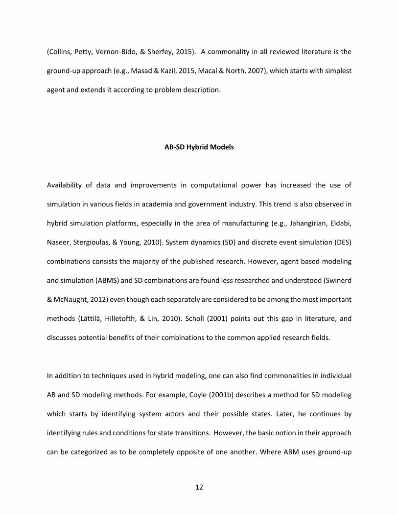
14
the system. Potential benefits from adapting MBSE is pointed out by a questionnaire conducted
by Pastrana (2014) where later, a roadmap is suggested for designing conceptual models of
distributed and hybrid simulation systems.
Figure 1 Vee- Model (INCOSE, 2011)
Systems Modeling Language (SysML)
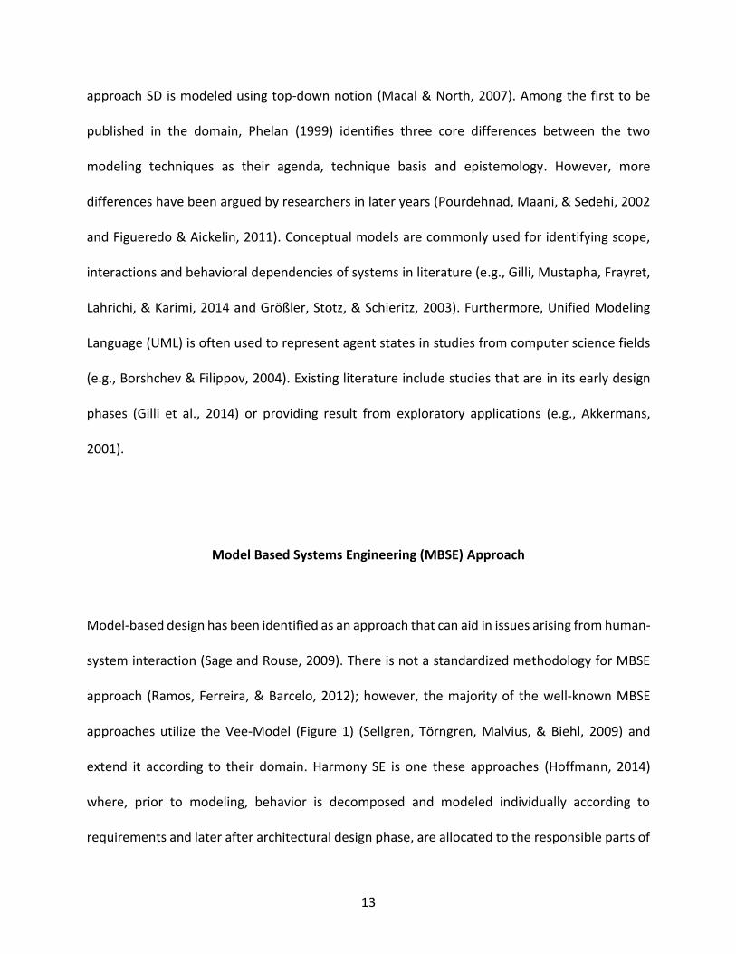
The holistic approach required in modeling complex systems are supported by four key modeling
facets, called pillars including nine diagrams, that consist of requirements, behavior, structure
and parametric relationships (Ramos et al. 2012). Figure 2 captures the representation of
diagrams published by Object Management Group (OMG) included in each pillar (Hause, 2006).
Although Package and Use-Case diagrams are not included in this representation they are also
considered a part of structure and behavior pillars, respectively.
15
Figure 2 Four Pillars of Model Based Systems Engineering (OMG, 2007)
Modeling and Simulation with SysML
Recent capabilities introduced by IBM’s Rational Rhapsody provides a platform for modeling
continues dynamics using SysML. According to Euler’s method (Huntsville, 2014) one can solve a
differential equation by approximating its solution at a discrete sub-division, referred to as steps,
of a continuous time interval. This can be expressed as:
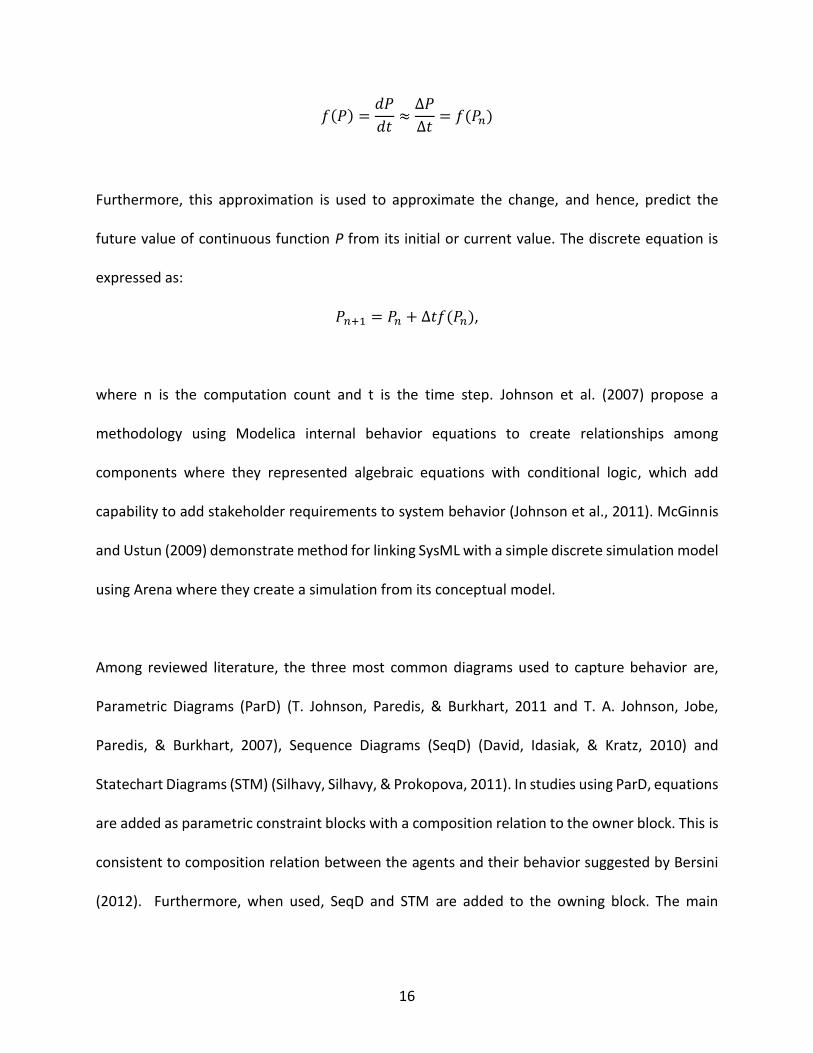
16
𝑓(𝑃) =𝑑𝑃
𝑑𝑡≈
∆𝑃
∆𝑡= 𝑓(𝑃𝑛)
Furthermore, this approximation is used to approximate the change, and hence, predict the
future value of continuous function P from its initial or current value. The discrete equation is
expressed as:
𝑃𝑛+1 = 𝑃𝑛 + ∆𝑡𝑓(𝑃𝑛),
where n is the computation count and t is the time step. Johnson et al. (2007) propose a
methodology using Modelica internal behavior equations to create relationships among
components where they represented algebraic equations with conditional logic, which add
capability to add stakeholder requirements to system behavior (Johnson et al., 2011). McGinnis
and Ustun (2009) demonstrate method for linking SysML with a simple discrete simulation model
using Arena where they create a simulation from its conceptual model.
Among reviewed literature, the three most common diagrams used to capture behavior are,
Parametric Diagrams (ParD) (T. Johnson, Paredis, & Burkhart, 2011 and T. A. Johnson, Jobe,
Paredis, & Burkhart, 2007), Sequence Diagrams (SeqD) (David, Idasiak, & Kratz, 2010) and
Statechart Diagrams (STM) (Silhavy, Silhavy, & Prokopova, 2011). In studies using ParD, equations
are added as parametric constraint blocks with a composition relation to the owner block. This is
consistent to composition relation between the agents and their behavior suggested by Bersini
(2012). Furthermore, when used, SeqD and STM are added to the owning block. The main

17
commonality among these studies is that the behaviors are created after the structure analysis
phase.
Majority of the proposed designs in literature-focusing on architectural design for different types
of simulation- revealed two distinct perspectives: proposing a design of the actual system and of
the conceptual model for the actual system’s simulation model. Studies from the first group, such
as the block definition diagram (BDD) suggested by Johnson et al. (2011), decompose the system
according to the actual components of the system. This is also common to studies suggesting a
multi–level approach for modeling hybrid models (Basole & Bodner, 2015). The decomposition
approach in studies belonging to the second group is based on the components of the model,
which is similar to approach used in software development. For example, Swinerd & McNaught
(2012) propose three design structures for SD-ABM models, which are decomposed according to
SD and ABM parts of the system. There are few studies that captured both perspectives such as
the mapping of domain and analysis meta-models proposed by Huang, Ramamurthy, & Mcginnis
(2007). Additional to SysML, studies using Unified Modeling Language (UML) (such as Bersini,
2012), are also reviewed to capture alternative proposals for developing a universal ontology.
Existing research on single type models showed SysML being used either to support conceptual
model development, similar to UML (Silhavy et al., 2011), or as foundation for models that could
be exported to other simulation software such as Modelica (Johnson, Jobe, Paredis, & Burkhart,
2007) or Arena (Mcginnis & Ustun, 2009).
18
Even though there is an increasing interest in literature, where SysML is used to support modeling
efforts, a gap exists in the domain, which adapts MBSE methodologies for modeling and
simulating systems within SysML. Furthermore, an approach which implicitly drives an agent-
based and system dynamics hybrid model of a system has not been provided. The few studies
published on agent-based and system dynamics hybrid modeling and simulation domain use
SysML to design the architectural components of a system’s model.
19
CHAPTER THREE: METHODOLOGY
Commonly used agent-based (AB) and system dynamics (SD) modeling techniques and
alternative workflow suggestions are summarized in Chapter 2. Even though each separately is
considered to be effective methods (Lättilä et al., 2010), there is very little research on agent-
based and system dynamics (AB-SD) combinations. Furthermore, majority of the work focuses
on model conceptualization and formulation and does not provide an approach that can
consistently be used all throughout the modeling and simulation workflow.
Computing power advancements paired with large amount of data collected over the years
significantly increase AB-SD modeling and simulation capabilities. However, these advancements
also increase the intricacy and the scale of modeled environments and introduce three core
challenges. First, high complexity is difficult to be included using the ground-up approach.
Second, the involvement of stakeholders-from various fields and backgrounds-introduces
additional needs and expectations, each facing unavoidable changes due to shifts in
environmental conditions. Finally, the need to maintain the coherency and efficiency of validated
models through structural or behavioral change requests that arise from emerging variables,
constraints or states. This research proposes an approach for modeling and maintaining AB-SD
hybrid models of systems using Systems Modeling Language (SysML).
20
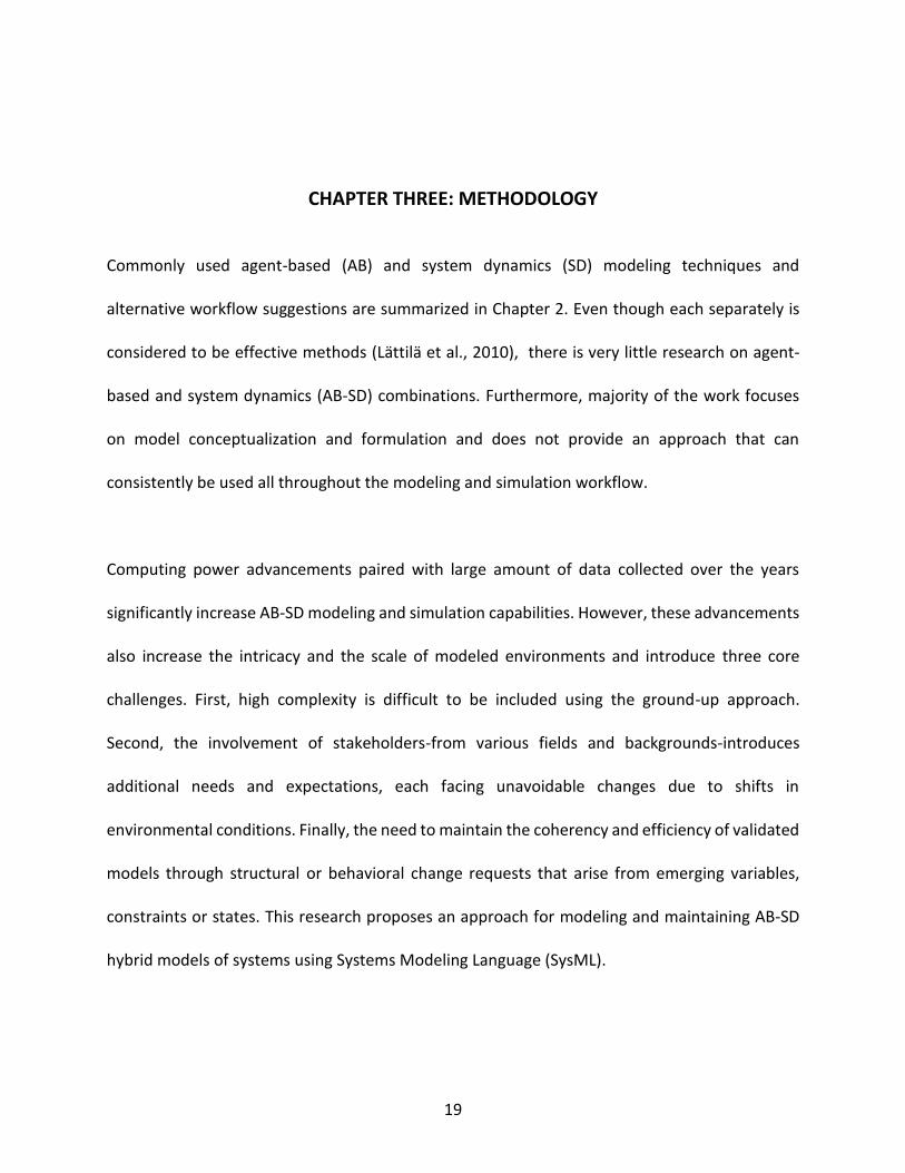
This section describes the methodology in four main phases. As shown in Figure 3, it starts with
requirements analysis and is followed by behavioral and structural design. Finally, it explains the
methods for validation and verification.
Figure 3 High-Level Methodology Process
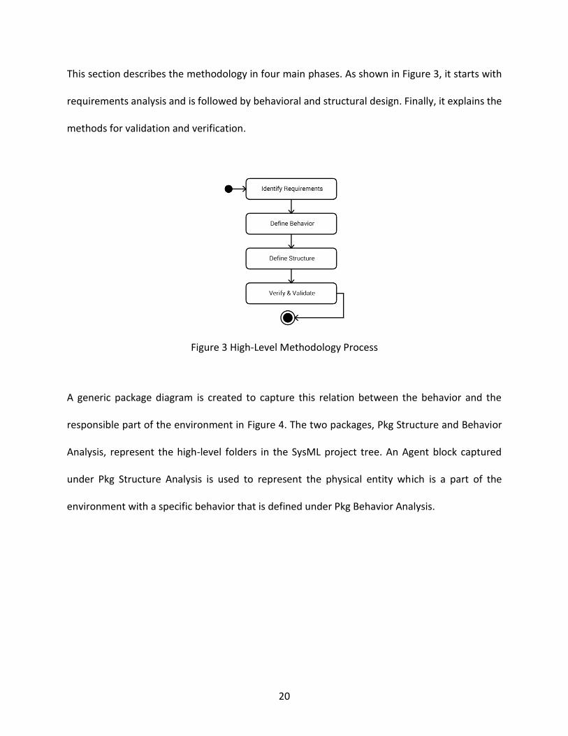
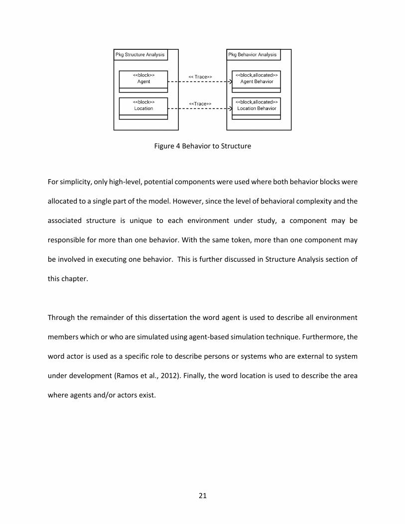
A generic package diagram is created to capture this relation between the behavior and the
responsible part of the environment in Figure 4. The two packages, Pkg Structure and Behavior
Analysis, represent the high-level folders in the SysML project tree. An Agent block captured
under Pkg Structure Analysis is used to represent the physical entity which is a part of the
environment with a specific behavior that is defined under Pkg Behavior Analysis.
21
Figure 4 Behavior to Structure
For simplicity, only high-level, potential components were used where both behavior blocks were
allocated to a single part of the model. However, since the level of behavioral complexity and the
associated structure is unique to each environment under study, a component may be
responsible for more than one behavior. With the same token, more than one component may
be involved in executing one behavior. This is further discussed in Structure Analysis section of
this chapter.
Through the remainder of this dissertation the word agent is used to describe all environment
members which or who are simulated using agent-based simulation technique. Furthermore, the
word actor is used as a specific role to describe persons or systems who are external to system
under development (Ramos et al., 2012). Finally, the word location is used to describe the area
where agents and/or actors exist.

22
Requirements Analysis
Grouping similar requirements is a common approach both in academia and private industry
(Friedenthal, Moore, & Steiner, 2009). Method uses five main groups for capturing the identified
capabilities and conditions expected from the model. The first two of five can be classified as
system-driven. These two groups include behavioral and structural requirements of the system.
The third and fourth groups can be classified as program-driven. Third group consists of
translation rules that are used for building the designed model in the selected simulation
environment or language. If the modeler is using the same two software consistently and neither
has gone through any significant updates, no change in the specifications is expected and
therefore can be imported for all new model designs. The fourth group captures model validation
and verification test specifications and includes a list of the variables and their expected values
that will be used within statistical tests. The final group can be classified as customer-driven. It is
used to list the variables, values of which must be collected for output analysis.
Different methodologies used in requirements analysis and management are not covered within
the scope of this dissertation. Further reading on the topic can be found in most SysML and MBSE
books (e.g. Weilkiens, 2006 and Friedenthal et al., 2009).
23
Define Behavior
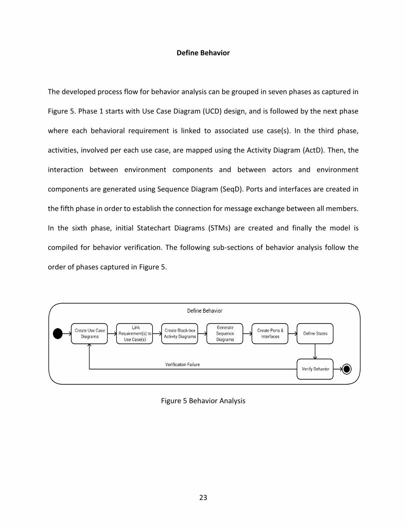
The developed process flow for behavior analysis can be grouped in seven phases as captured in
Figure 5. Phase 1 starts with Use Case Diagram (UCD) design, and is followed by the next phase
where each behavioral requirement is linked to associated use case(s). In the third phase,
activities, involved per each use case, are mapped using the Activity Diagram (ActD). Then, the
interaction between environment components and between actors and environment
components are generated using Sequence Diagram (SeqD). Ports and interfaces are created in
the fifth phase in order to establish the connection for message exchange between all members.
In the sixth phase, initial Statechart Diagrams (STMs) are created and finally the model is
compiled for behavior verification. The following sub-sections of behavior analysis follow the
order of phases captured in Figure 5.
Figure 5 Behavior Analysis

24
Create Use Case Diagrams (UCD)
UCD is used to identify environment boundaries, scope, and model behavior and any internal and
external interactions defined within the project scope. A flow chart is developed for creating the
UCD. First the modeler identifies actors, their relation with the system and the types of their
behavior, referred to as functions. Later, similar actions are repeated to identify the emphasis,
and impact of location conditions and events if any are included within the environment
boundaries.
The process starts by adding all members of environment, which are involved in, have impact on
or simply observe outcomes. These can include stakeholders, external systems, agents and even
locations other than the one considered within the focus. Later, by iterating a series of decisions,
the modeler identifies the actors’ relations to the modeled system and their time or SD driven
behaviors. Agents who are identified as a part of the environment are not added to UCD as actors.
However, their behaviors are added as functions within the system boundary box. Later in section
Structure Analysis, these are added as a part of the environment and designed behaviors are
allocated to each responsible party.
Location of agents may play an important role in the design depending on the type of
environment scenario. For example, studies focusing on influenza outbreak (eg. Lukens et al.,
2014) often derive contact rate from the distance between agents. In such cases, location of each
agent is considered as a factor impacting experiment results and therefore may be included in
25
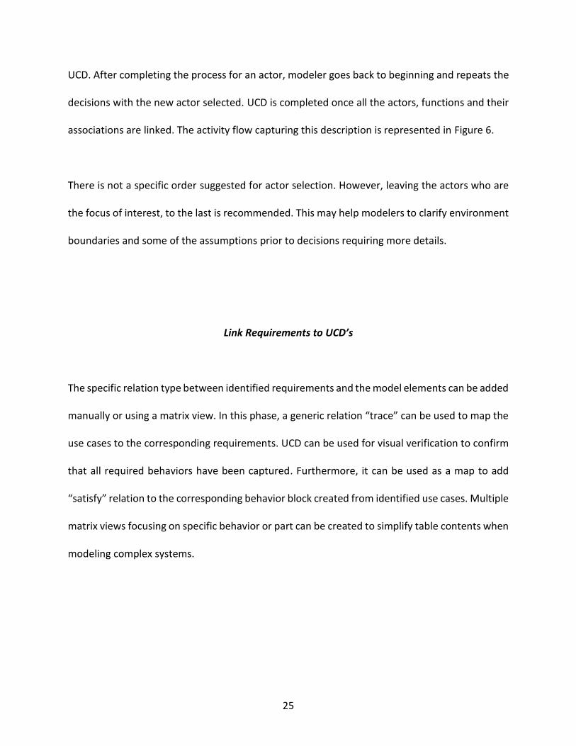
UCD. After completing the process for an actor, modeler goes back to beginning and repeats the
decisions with the new actor selected. UCD is completed once all the actors, functions and their
associations are linked. The activity flow capturing this description is represented in Figure 6.
There is not a specific order suggested for actor selection. However, leaving the actors who are
the focus of interest, to the last is recommended. This may help modelers to clarify environment
boundaries and some of the assumptions prior to decisions requiring more details.
Link Requirements to UCD’s
The specific relation type between identified requirements and the model elements can be added
manually or using a matrix view. In this phase, a generic relation “trace” can be used to map the
use cases to the corresponding requirements. UCD can be used for visual verification to confirm
that all required behaviors have been captured. Furthermore, it can be used as a map to add
“satisfy” relation to the corresponding behavior block created from identified use cases. Multiple
matrix views focusing on specific behavior or part can be created to simplify table contents when
modeling complex systems.

26
Figure 6 Use Case Diagram Development Process

27
Create Activity Diagrams (ActD)
The activity diagram is used to capture the sequence of actions that needs to be executed in
order to satisfy the goal defined by a use case (Weilkiens, 2006). The path of sequence execution
is represented using control or object flows depending on the type of information necessary for
executing an activity. If a system consists of activities common to more than one use case, they
can be designed either explicitly as an operation or in groups as behaviors. Furthermore, an
activity can be an action state or a message. Although multiple actions can be represented as
embedded code within a single activity, it is not recommended. This method would not simplify
the modeling of system behavior complexity, therefore would eliminate the benefits that can be
achieved using MBSE approach.
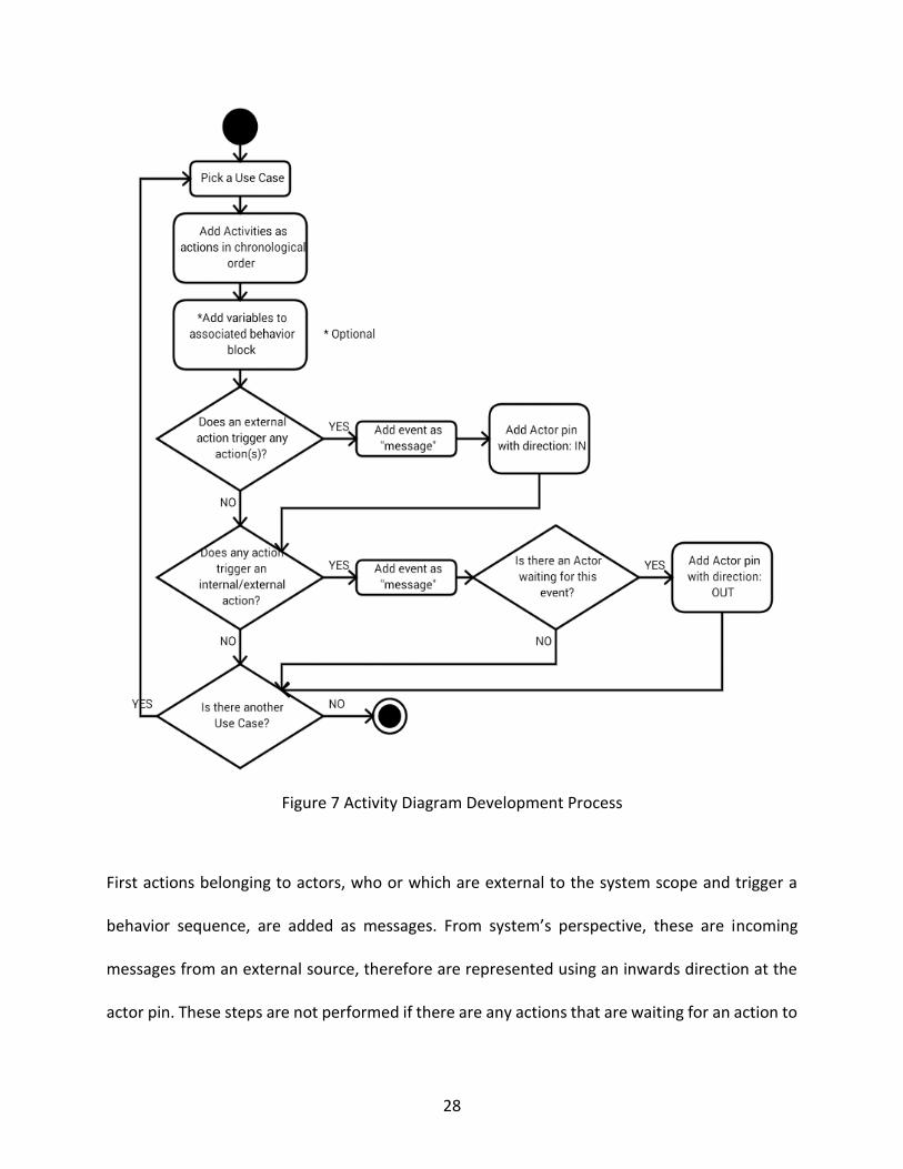
Developed flow (Figure 7) starts by adding the actions of the selected use case and placing them
in the diagram in a sequential order. A decision, fork and join nodes are later added if necessary
to represent conditional reactions of the system. In the third step, the variables, which will be
used either at the decision nodes or within actions, are added to the associated behavior block.
Common variables must be added only once and to the responsible behavior block. For example,
simulation time variable would only be added to the update time behavior block. Later during
structural design these common variables will be allocated to all parts of the system. A star is
added to this step to indicate that it is optional. The modeler can also use the sequence diagrams
to identify variables and add them to the associated behavior block. Remaining steps focus on
capturing internal and external message exchange.
28
Figure 7 Activity Diagram Development Process
First actions belonging to actors, who or which are external to the system scope and trigger a
behavior sequence, are added as messages. From system’s perspective, these are incoming
messages from an external source, therefore are represented using an inwards direction at the
actor pin. These steps are not performed if there are any actions that are waiting for an action to

29
be completed by a different behavior block within the system. The waited actions are captured
only at the ActD of the behavior block responsible of performing the action. Therefore, when
modeling systems with complex behavior, activity diagrams must be created simultaneously.
Instead of waiting to complete one ActD, when identified, the required action can be added as a
message to the ActD of the responsible behavior block. Last group of steps focuses on identifying
and adding such actions as messages. Process flow of the described method is captured in Figure
7.
Required ActDs such as “update_time” or “update_dynamics” can be used to start the modeling
in this phase. If this is the first time this methodology is being used, modeler would create them
manually and save the project. If not, a previously saved project with only the two use cases and
their behavior blocks, can be imported using the “Add to model” menu option in Rhapsody (IBM,
2014).
The ActD for “update_time” behavior consists of one action, “increment_clock”. Furthermore, it
is responsible of starting the overall system execution and updating the internal clock. As a result
it consists of two message actions and one action with embedded code that will increment the
clock (Figure 8). A variable named “Tnow” is added to the block representing the time of the
simulation in days.
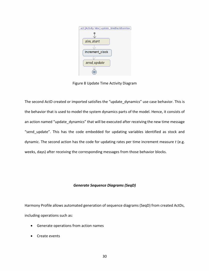
30
Figure 8 Update Time Activity Diagram
The second ActD created or imported satisfies the “update_dynamics” use case behavior. This is
the behavior that is used to model the system dynamics parts of the model. Hence, it consists of
an action named “update_dynamics” that will be executed after receiving the new time message
“send_update”. This has the code embedded for updating variables identified as stock and
dynamic. The second action has the code for updating rates per time increment measure t (e.g.
weeks, days) after receiving the corresponding messages from those behavior blocks.
Generate Sequence Diagrams (SeqD)
Harmony Profile allows automated generation of sequence diagrams (SeqD) from created ActDs,
including operations such as:
Generate operations from action names
Create events
31
Create interface
Add corresponding operation and event realizations (Hoffmann, 2014).
One or more SeqDs can be created for a behavior block. However, to maintain modularity at least
one SeqD per behavior block should be created. If Harmony profile is not used for SeqD
generations, each listed operation has to be completed manually. Later in the SeqD operations
and events should be assigned to message and event tools, simultaneously, as realizations. Only
the messages exchanged between the system and actors are shown in initial SeqDs since these
are created from the black-box activity diagrams. Internal messages are added to the SeqD after
the actions are allocated to the responsible system parts during architectural design phase.
Depending on the level of detail required, the behavior and conditional rules can be planned
using SeqD. Although this is not required, it would lay the grounds for mapping the rules for state-
based behavior and support designing efforts. Rhapsody diagram tools can be used to add
conditions and logic for operation sequence. All types of operator based interactions added to
SeqD are only added as a visual guidance and are not included in the compiled simulation
execution file (IBM, 2014).
Create Ports and Interfaces
Similar to SeqD generation, ports and interfaces can be created automatically using the Harmony
toolkit. This option will move all external events to corresponding interfaces and add receptions

32
to the receiving party. Finally, it will add parts of the behavior block and interacting actors to
capture their communication using an Internal Block Diagram (IBD). Each behavior block created
up until this phase will have its own IBD. The main purpose is to identify the specific behavior
block, where the overall system is required to interact with an actor in the environment
surrounding itself.
Define States
In behavioral design phase decomposed blocks are treated individually. Therefore one state
diagram is created for each behavior block. The states and transition conditions are added
according to the logic identified in SeqDs. The modeler can embed the code for operations during
any state after SeqD design. However, all remaining code should be embedded during state
definition. In order to maintain modularity, elements from the Rhapsody toolbar should be used
rather than embedding complex conditions or loops within one operation.
“UC_update_time” is designed to be used for representing the internal clock of the system. As a
result, it is set to be incremented once per day continuously. However, for simulations that are
time bounded, an end state can be added using a conditional trigger for the final transition. As
captured in Figure 9, only one of the operations defined in Figure 8 Update Time is used at this
step. Any internal messages such as “sim_start” or “send_update” are added after the system is
decomposed to its parts during structure analysis phase.
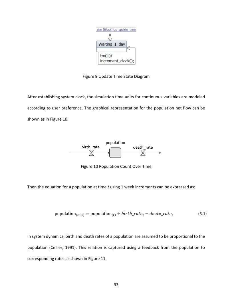
33
Figure 9 Update Time State Diagram
After establishing system clock, the simulation time units for continuous variables are modeled
according to user preference. The graphical representation for the population net flow can be
shown as in Figure 10.
Figure 10 Population Count Over Time
Then the equation for a population at time t using 1 week increments can be expressed as:
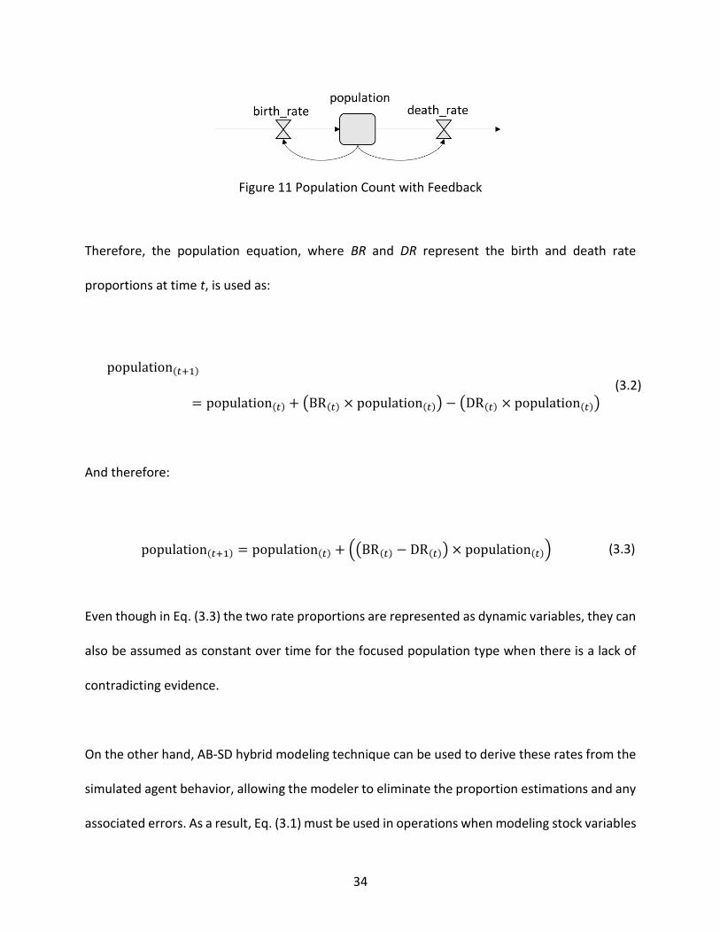
In system dynamics, birth and death rates of a population are assumed to be proportional to the
population (Cellier, 1991). This relation is captured using a feedback from the population to
corresponding rates as shown in Figure 11.
population(𝑡+1) = population(𝑡) + 𝑏𝑖𝑟𝑡ℎ_𝑟𝑎𝑡𝑒𝑡 − 𝑑𝑒𝑎𝑡𝑒_𝑟𝑎𝑡𝑒𝑡 (3.1)
34
Figure 11 Population Count with Feedback
Therefore, the population equation, where BR and DR represent the birth and death rate
proportions at time t, is used as:
And therefore:
Even though in Eq. (3.3) the two rate proportions are represented as dynamic variables, they can
also be assumed as constant over time for the focused population type when there is a lack of
contradicting evidence.
On the other hand, AB-SD hybrid modeling technique can be used to derive these rates from the
simulated agent behavior, allowing the modeler to eliminate the proportion estimations and any
associated errors. As a result, Eq. (3.1) must be used in operations when modeling stock variables
population(𝑡+1)
= population(𝑡) + (BR(𝑡) × population(𝑡)) − (DR(𝑡) × population(𝑡))
(3.2)
population(𝑡+1) = population(𝑡) + ((BR(𝑡) − DR(𝑡)) × population(𝑡)) (3.3)

35
that depend on agent behavior, such as “update_population()”. In order to maintain validity after
this elimination, the modeler is required to provide more detailed information about the
population at time 0 compared to SD modeling.
Behavior Verification
Similar to previous phases, the verification of decomposed behavior is done individually. First,
developed model is compiled using simulated time in MSVC environment with C++ language and
any possible issues are fixed. Later the program is executed and the individual behavior of each
block is observed using simulated statecharts and sequence diagrams (IBM, 2014). As the final
step, properties of all variables are checked for any errors.
Overall, the purpose of behavior analysis can be summarized as following:
Identify system requirements
Identify system scope and boundaries
Identify the modularized actions and reactions of the system to the external triggers
Identify its interaction with the surrounding environment and conditions
Derive resulting behavior from findings gathered above for verification

36
Define Structure
The process flow for structure analysis is grouped in three phases that are system decomposition,
behavior allocation and verification and validation as captured in Figure 12. Behavior allocation
is further completed in four sub-phases where names have been kept the same on purpose to
point out the shared diagrams between the two analyses.
Figure 12 Structure Analysis
Create Block Definition Diagrams
In literature review, the two approaches used in system decomposition for system modeling were
discussed. During initial research efforts the selected system was decomposed according to its
conceptual model parts. (Soyler Akbas, Mykoniatis, Angelopoulou, & Karwowski, 2014). Hence,
the training system was decomposed as Agent-Based Model and System Dynamics Model (Figure
13). However as SD and ABM parts were further decomposed; behavior allocation and
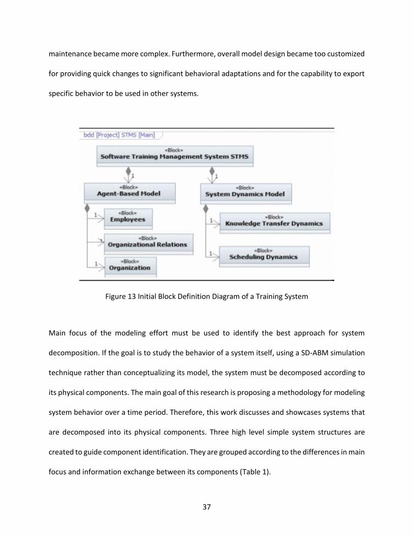
37
maintenance became more complex. Furthermore, overall model design became too customized
for providing quick changes to significant behavioral adaptations and for the capability to export
specific behavior to be used in other systems.
Figure 13 Initial Block Definition Diagram of a Training System
Main focus of the modeling effort must be used to identify the best approach for system
decomposition. If the goal is to study the behavior of a system itself, using a SD-ABM simulation
technique rather than conceptualizing its model, the system must be decomposed according to
its physical components. The main goal of this research is proposing a methodology for modeling
system behavior over a time period. Therefore, this work discusses and showcases systems that
are decomposed into its physical components. Three high level simple system structures are
created to guide component identification. They are grouped according to the differences in main
focus and information exchange between its components (Table 1).

38
Table 1 System Decomposition Types
Decomposition Type Information Type Explanation
One Way Agents to Location
Main system focus is the location
Common location shared by all agents
Changes in environment do not impact agent behavior
Changes in agent behavior impact the location
One Way Location to Agents
Main system focus is agents
Unique location per agent
Changes in location impact agent behavior
Changes in agent behavior do not impact their location
Two Way Agents to Location & Location to Agents
System focus is both
Common location shared by all agents
Changes in environment impact agent behavior
Changes in agent behavior impact their environment
39
The “Agent” is used to represent unique objects, people, locations, which can be grouped under
one goal. Similarly, “Location” represents a physical or conceptual location common or unique to
agents. Both can include SD models. With the same token, both or sub-parts of both can be
modeled as agents in AB models. This is further explained in the following section under each
category.
Decomposition Type I
This type consists of models focusing on locational factors changing due to agent behavior
independent of the location. Both location and agent can represent more than one unique part
of the system. However, this layout assumes no interaction between individuals existing in
different locations. The method provides the use of this structure only if there is a possible scope
change in the future to include agents within the focus or they share conditions that impact both
of their behavior in the environment over time. If not, Agents must be represented as actors
under UCD, as externals only impacting the system. The farmers’ impact on ecological carbon
and nitrogen stock model introduced by Gaube et al., 2009 is an example of this type. In this
study one can see the impact of farmers’ work on the flows however the impact of nitrogen and
carbon on an individual farmer is negligibly small and therefore not included.
40
Decomposition Type II
Type II can be used when the system focus is completely opposite to described in Type I. Hence,
must be used when simulating systems where the change in an agent is driven by the changes in
its location or locations. This design assumes each location is unique to an agent therefore, the
system focus does not include location based interactions between agents. Simple supply-chain
models can be given as examples of this type. Manufacturers’ decision making process at a micro
level driven from the status of the raw material in their area of service can be modeled using this
structure.
Decomposition Type III
In systems that require two way dependencies between its agent(s) and location(s) the model
must be structured with parallel hierarchy using type III. This structure can allow actors to share
the existing location conditions or resources and locations to drive their change based on
individual and combined behavior simultaneously. Most of the population studies can be given
as examples in this group such as the model proposed by Chaim, 2008. Using this structure,
location dependent agents with unique SD or AB behaviors can be modeled at a micro level where
their impact on the population can be modeled at a macro level under location.

41
Complex Decompositions
A combination out of the three proposed decomposition types can be used when modeling
complex systems. Systems should be studied according to interdependencies among its
components and the project scope to find the most suitable combination. For example a supply
chain system including buyers, product manufacturers and raw material manufactures shared by
all high level manufacturers can be decomposed using two Type II and one Type I decomposition
structures as shown in Figure 14. However, if the original scope does not include the impact of
factory locations they can be eliminated from the design.
Figure 14 Complex Supply Chain System Decomposition
This methodology can be useful for long term projects as they can be more open to project scope
changes. Such a system model which originally consists of a single type, can be later extended to
include micro details.
42
Allocate Behavior
Modeler can merge behavior designed in the previous section with the main system block after
the system is decomposed to its components. This action will copy all operations and attributes
into the main system block with a trace relation added, linking it back to the original behavior
block. Later, the behavior is allocated to each responsible component using the graphs previously
created or duplicated. This is further explained in the following sections. Similar to behavior
analysis, the modeler can choose to complete the remaining phases either manually or by using
Harmony profile tools.
Create White-Box Activity Diagrams (ActD)
In this phase, first, previously created ActDs are duplicated and renamed as White-box ActDs.
Later, a swim lane is added for each system part and operations are placed-by moving- under the
responsible block.
Generate Sequence Diagrams (SeqD) and Create Ports and Interfaces
After each behavior is allocated to the responsible part of the system Harmony profile can be
used for generating the SeqDs and for creating the ports and event interfaces. This is executed
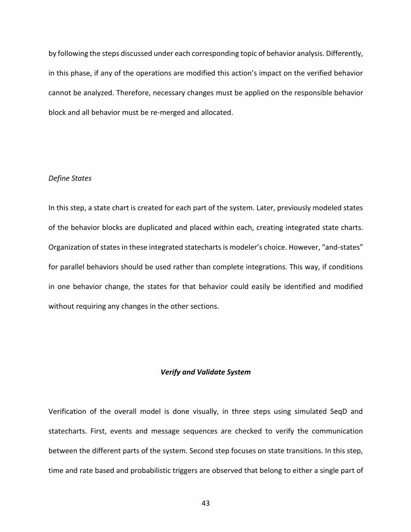
43
by following the steps discussed under each corresponding topic of behavior analysis. Differently,
in this phase, if any of the operations are modified this action’s impact on the verified behavior
cannot be analyzed. Therefore, necessary changes must be applied on the responsible behavior
block and all behavior must be re-merged and allocated.
Define States
In this step, a state chart is created for each part of the system. Later, previously modeled states
of the behavior blocks are duplicated and placed within each, creating integrated state charts.
Organization of states in these integrated statecharts is modeler’s choice. However, “and-states”
for parallel behaviors should be used rather than complete integrations. This way, if conditions
in one behavior change, the states for that behavior could easily be identified and modified
without requiring any changes in the other sections.
Verify and Validate System
Verification of the overall model is done visually, in three steps using simulated SeqD and
statecharts. First, events and message sequences are checked to verify the communication
between the different parts of the system. Second step focuses on state transitions. In this step,
time and rate based and probabilistic triggers are observed that belong to either a single part of

44
the system or to randomly selected objects of parts whose multiplicities are more than one. In
the final step of verification, function executions are checked by observing the change in variable
values over time.
Output variables identified for validation during requirements analysis phase are used to conduct
statistical output analysis. A hypothesis test, such as difference of means, is used to calculate the
significance of difference between the model output and collected data from the real system.
45
CHAPTER FOUR: METHODOLOGY VERIFICATION
Two challenges were faced when the methodology was applied using IBM’s Rational Rhapsody.
This section describes these issues and proposes solutions for overcoming these limitations. It
starts with probabilistic behavior under Variability and later continues with time synchronization.
Variability
Rhapsody is not designed as a simulation tool and default C++ package does not come with a
predefined math library functions. Therefore a random number following a specific distribution
cannot be generated, except for uniform distribution. To eliminate this limitation a
“generate_variate” behavior is created for systems which consists of behaviors with defined
distributions. This behavior block includes calculations adapted from random variate generation
techniques as functions.
For example, the associated variables and operations allocated to a “rate” block and the
pseudocode of the algorithm for creating duration based state change that is exponentially
distributed with a rate 0.1 per day are presented in Figure 15 and Algorithm 1, respectively.

46
Figure 15 Rate Block Values and Operations
Algorithm 1 Generate Timeout
1: Date: Day count at timeout
2: Ln[100]: Array storing -ln(i/100) where int i ~ U(0,100)
3: U: Generated integer ~ U(0,100)
4: Uni: Value at Ln[U]
5: While on transition between states
6: if next state has distributed transition then
7: Generate uniform variable U
8: Set Uni Ln[U]
9: Calculate exponential variate Date with rate 0.1
10: end if
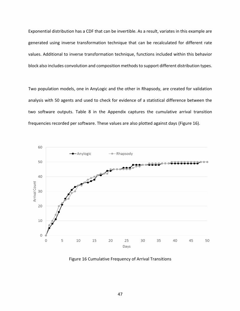
47
Exponential distribution has a CDF that can be invertible. As a result, variates in this example are
generated using inverse transformation technique that can be recalculated for different rate
values. Additional to inverse transformation technique, functions included within this behavior
block also includes convolution and composition methods to support different distribution types.
Two population models, one in AnyLogic and the other in Rhapsody, are created for validation
analysis with 50 agents and used to check for evidence of a statistical difference between the
two software outputs. Table 8 in the Appendix captures the cumulative arrival transition
frequencies recorded per software. These values are also plotted against days (Figure 16).
Figure 16 Cumulative Frequency of Arrival Transitions

48
In cases of correlated outputs, such as this, mean of differences recorded for t = 0, 1…, 50 can be
used for testing statistical difference. Where Xt and Yt represent the outputs recorded on day, t,
from AnyLogic and Rhapsody, respectively, the test criteria are as follows:
𝐻0: 𝐷𝑡 = 0, 𝑤ℎ𝑒𝑟𝑒 𝐷𝑡 = 𝑋𝑡 − 𝑌𝑡
𝐻𝑎: 𝐷𝑡 ≠ 0
�̅� =1
50∑ 𝐷𝑡
50
𝑡=1
≅ −0.27451
𝑆𝐷 = √1
(50 ∗ 49)∑(D𝑡 − �̅�)2
50
𝑡=1
≅ 1.3723
Tcalculation ≅ −0.200
T0.025,49 ≅ 1.96
Since 𝑇𝑐𝑎𝑙𝑐𝑢𝑙𝑎𝑡𝑖𝑜𝑛 falls within ±1.96 there is not significant evidence supporting a statistical
difference between the two outputs from AnyLogic and Rhapsody.
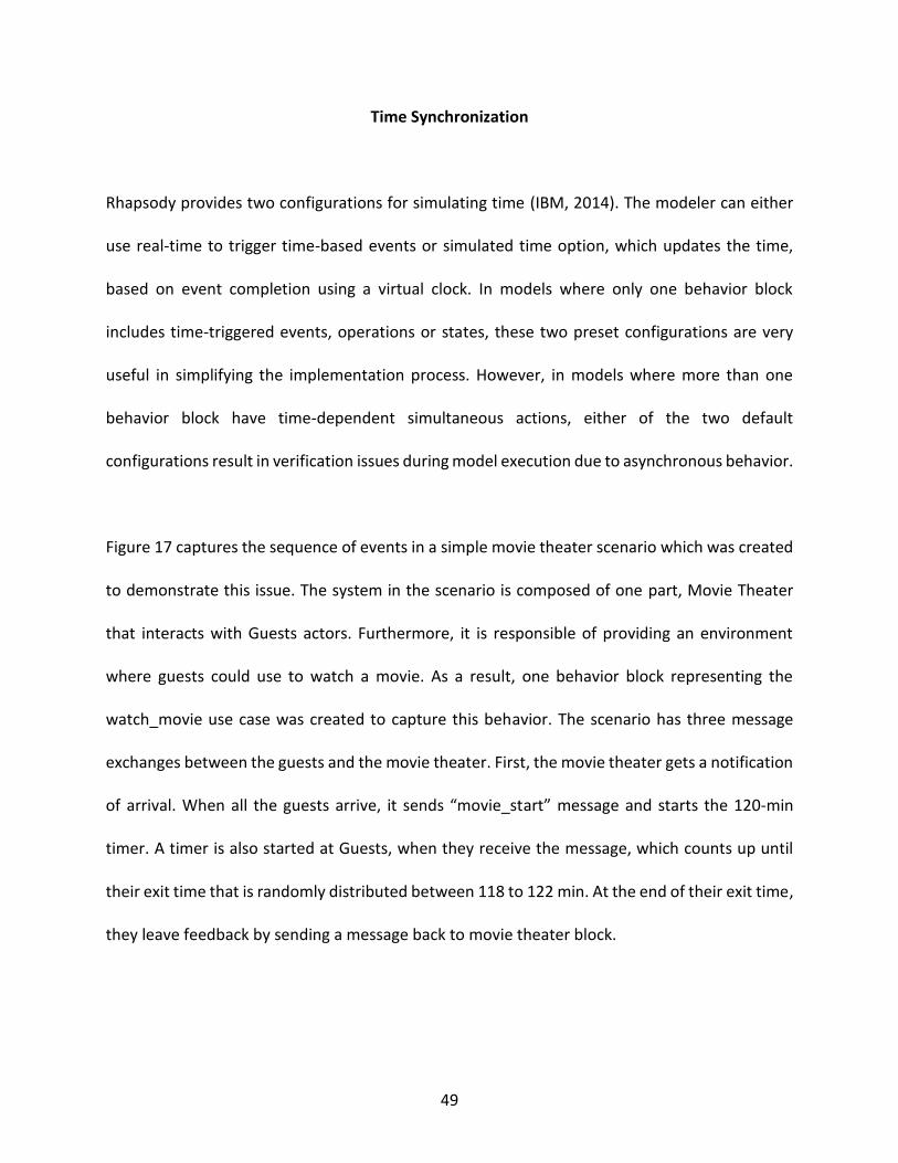
49
Time Synchronization
Rhapsody provides two configurations for simulating time (IBM, 2014). The modeler can either
use real-time to trigger time-based events or simulated time option, which updates the time,
based on event completion using a virtual clock. In models where only one behavior block
includes time-triggered events, operations or states, these two preset configurations are very
useful in simplifying the implementation process. However, in models where more than one
behavior block have time-dependent simultaneous actions, either of the two default
configurations result in verification issues during model execution due to asynchronous behavior.
Figure 17 captures the sequence of events in a simple movie theater scenario which was created
to demonstrate this issue. The system in the scenario is composed of one part, Movie Theater
that interacts with Guests actors. Furthermore, it is responsible of providing an environment
where guests could use to watch a movie. As a result, one behavior block representing the
watch_movie use case was created to capture this behavior. The scenario has three message
exchanges between the guests and the movie theater. First, the movie theater gets a notification
of arrival. When all the guests arrive, it sends “movie_start” message and starts the 120-min
timer. A timer is also started at Guests, when they receive the message, which counts up until
their exit time that is randomly distributed between 118 to 122 min. At the end of their exit time,
they leave feedback by sending a message back to movie theater block.
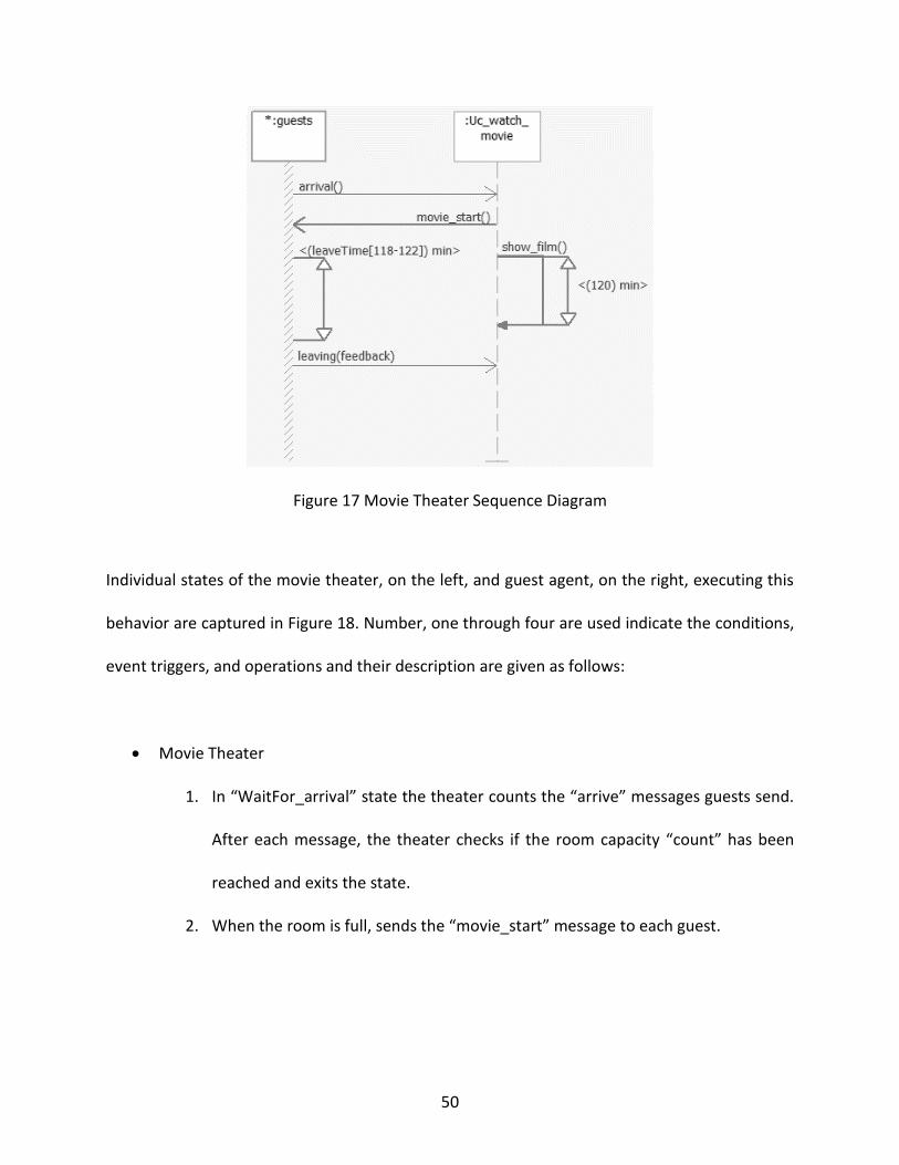
50
Figure 17 Movie Theater Sequence Diagram
Individual states of the movie theater, on the left, and guest agent, on the right, executing this
behavior are captured in Figure 18. Number, one through four are used indicate the conditions,
event triggers, and operations and their description are given as follows:
Movie Theater
1. In “WaitFor_arrival” state the theater counts the “arrive” messages guests send.
After each message, the theater checks if the room capacity “count” has been
reached and exits the state.
2. When the room is full, sends the “movie_start” message to each guest.

51
3. “ShowMovie” state stays active for 120 minutes. This behavior is assigned using a
time trigger function “tm(duration)”. During this state it starts collecting the
feedback from guests who are leaving before the movie ends.
4. Waits until feedback is collected from all guests
Guest Actor
1. Each guest notifies the theater when they arrive.
2. They wait for all guests to arrive.
3. They leave the movie theater randomly between 118 to 122 minutes after the
movie starts.
4. They give a feedback with a score between 1 and 10 before exiting.

52
Figure 18 Movie Theater and Guest Agent Behavior
Figure 19 shows the expected sequence of events and states of guest actor and the movie
theater. Verification of the model includes checking the correctness of the event sequence
indicated by the rectangle box. The correct behavior is guests with “leaveTime” less than 120
minutes sending their feedback before and the remaining sending it after the movie is over. The
scenario was executed 31 times representing a day with 11 shows using a 30 guest capacity.
However, due to generated random numbers being the same, no difference was observed
between 31 iterations.

53
Figure 19 Expected Output
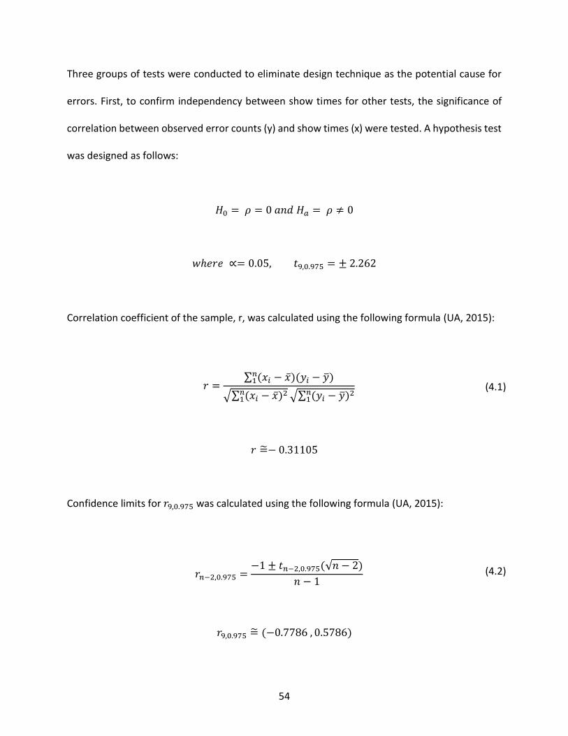
54
Three groups of tests were conducted to eliminate design technique as the potential cause for
errors. First, to confirm independency between show times for other tests, the significance of
correlation between observed error counts (y) and show times (x) were tested. A hypothesis test
was designed as follows:
𝐻0 = 𝜌 = 0 𝑎𝑛𝑑 𝐻𝑎 = 𝜌 ≠ 0
𝑤ℎ𝑒𝑟𝑒 ∝= 0.05, 𝑡9,0.975 = ± 2.262
Correlation coefficient of the sample, r, was calculated using the following formula (UA, 2015):
𝑟 =̃− 0.31105
Confidence limits for 𝑟9,0.975 was calculated using the following formula (UA, 2015):
𝑟9,0.975 =̃ (−0.7786 , 0.5786)
𝑟 =∑ (𝑥𝑖 − �̅�)(𝑦𝑖 − �̅�)𝑛
1
√∑ (𝑥𝑖 − �̅�)2𝑛1 √∑ (𝑦𝑖 − �̅�)2𝑛
1
(4.1)
𝑟𝑛−2,0.975 =−1 ± 𝑡𝑛−2,0.975(√𝑛 − 2)
𝑛 − 1 (4.2)
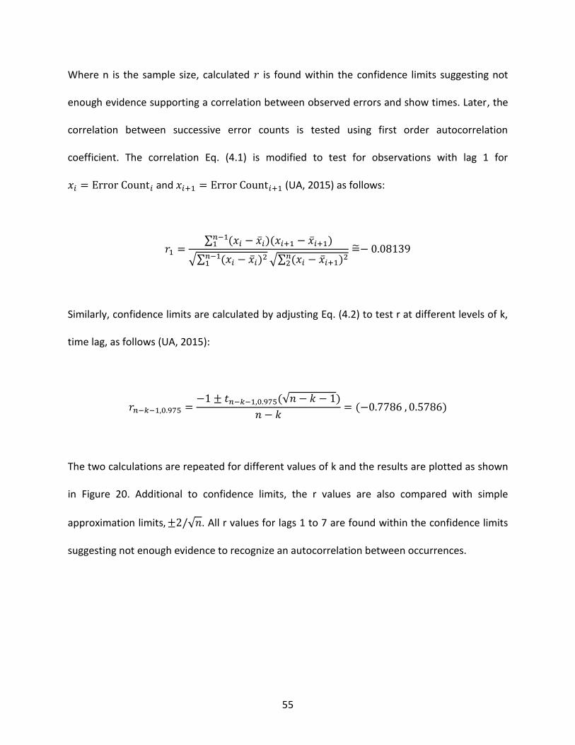
55
Where n is the sample size, calculated 𝑟 is found within the confidence limits suggesting not
enough evidence supporting a correlation between observed errors and show times. Later, the
correlation between successive error counts is tested using first order autocorrelation
coefficient. The correlation Eq. (4.1) is modified to test for observations with lag 1 for
𝑥𝑖 = Error Count𝑖 and 𝑥𝑖+1 = Error Count𝑖+1 (UA, 2015) as follows:
𝑟1 =∑ (𝑥𝑖 − �̅�𝑖)(𝑥𝑖+1 − �̅�𝑖+1)𝑛−1
1
√∑ (𝑥𝑖 − �̅�𝑖)2𝑛−11 √∑ (𝑥𝑖 − �̅�𝑖+1)2𝑛
2
=̃− 0.08139
Similarly, confidence limits are calculated by adjusting Eq. (4.2) to test r at different levels of k,
time lag, as follows (UA, 2015):
𝑟𝑛−𝑘−1,0.975 =−1 ± 𝑡𝑛−𝑘−1,0.975(√𝑛 − 𝑘 − 1)
𝑛 − 𝑘= (−0.7786 , 0.5786)
The two calculations are repeated for different values of k and the results are plotted as shown
in Figure 20. Additional to confidence limits, the r values are also compared with simple
approximation limits, ±2/√𝑛. All r values for lags 1 to 7 are found within the confidence limits
suggesting not enough evidence to recognize an autocorrelation between occurrences.
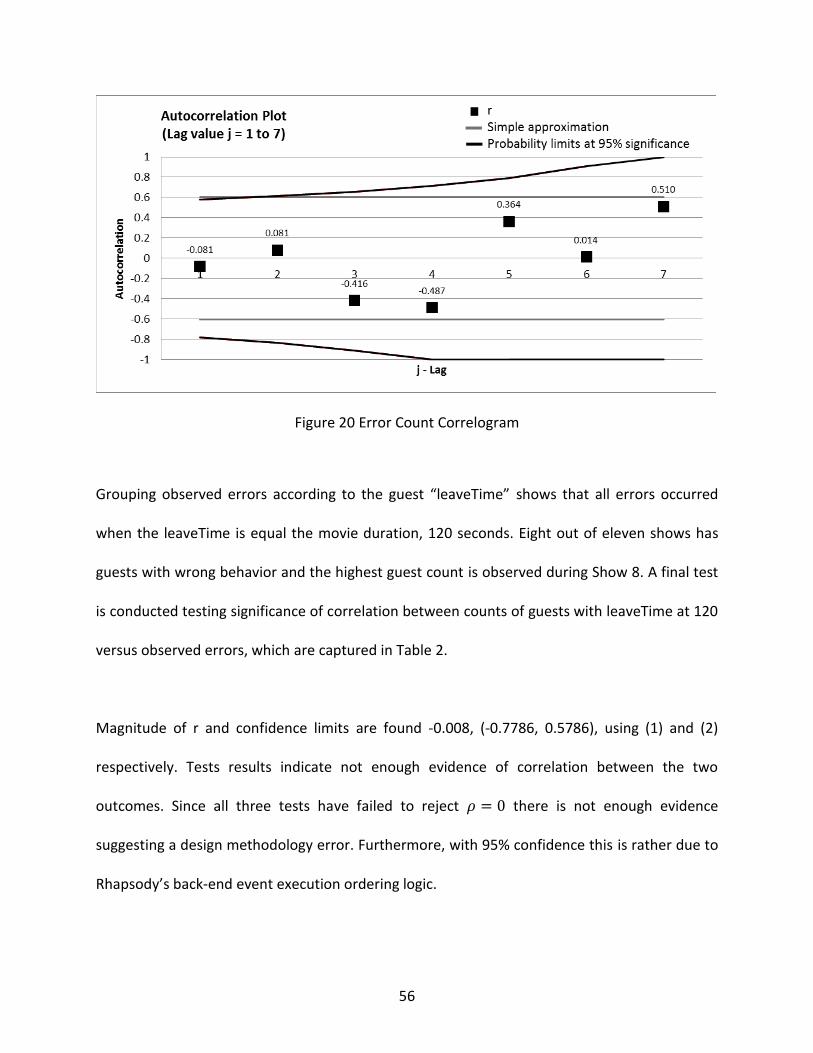
56
Figure 20 Error Count Correlogram
Grouping observed errors according to the guest “leaveTime” shows that all errors occurred
when the leaveTime is equal the movie duration, 120 seconds. Eight out of eleven shows has
guests with wrong behavior and the highest guest count is observed during Show 8. A final test
is conducted testing significance of correlation between counts of guests with leaveTime at 120
versus observed errors, which are captured in Table 2.
Magnitude of r and confidence limits are found -0.008, (-0.7786, 0.5786), using (1) and (2)
respectively. Tests results indicate not enough evidence of correlation between the two
outcomes. Since all three tests have failed to reject 𝜌 = 0 there is not enough evidence
suggesting a design methodology error. Furthermore, with 95% confidence this is rather due to
Rhapsody’s back-end event execution ordering logic.
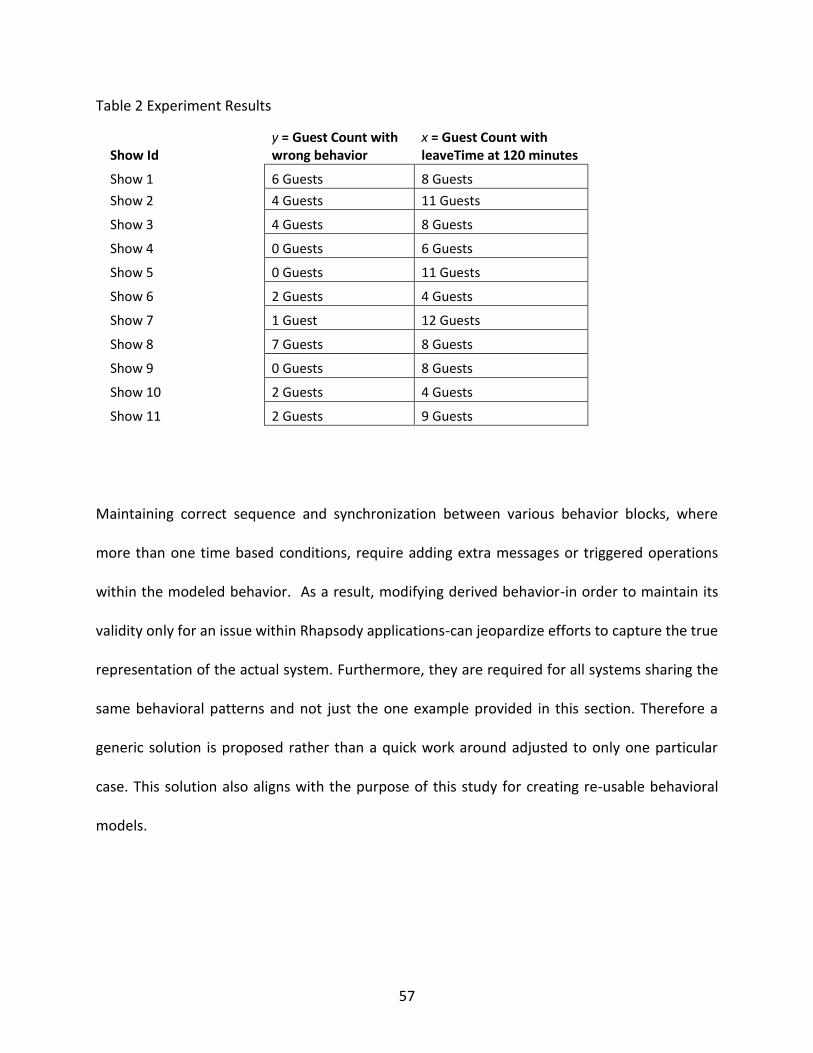
57
Table 2 Experiment Results
Show Id y = Guest Count with wrong behavior
x = Guest Count with leaveTime at 120 minutes
Show 1 6 Guests 8 Guests
Show 2 4 Guests 11 Guests
Show 3 4 Guests 8 Guests
Show 4 0 Guests 6 Guests
Show 5 0 Guests 11 Guests
Show 6 2 Guests 4 Guests
Show 7 1 Guest 12 Guests
Show 8 7 Guests 8 Guests
Show 9 0 Guests 8 Guests
Show 10 2 Guests 4 Guests
Show 11 2 Guests 9 Guests
Maintaining correct sequence and synchronization between various behavior blocks, where
more than one time based conditions, require adding extra messages or triggered operations
within the modeled behavior. As a result, modifying derived behavior-in order to maintain its
validity only for an issue within Rhapsody applications-can jeopardize efforts to capture the true
representation of the actual system. Furthermore, they are required for all systems sharing the
same behavioral patterns and not just the one example provided in this section. Therefore a
generic solution is proposed rather than a quick work around adjusted to only one particular
case. This solution also aligns with the purpose of this study for creating re-usable behavioral
models.
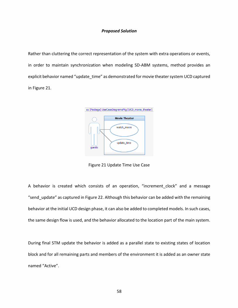
58
Proposed Solution
Rather than cluttering the correct representation of the system with extra operations or events,
in order to maintain synchronization when modeling SD-ABM systems, method provides an
explicit behavior named “update_time” as demonstrated for movie theater system UCD captured
in Figure 21.
Figure 21 Update Time Use Case
A behavior is created which consists of an operation, “increment_clock” and a message
“send_update” as captured in Figure 22. Although this behavior can be added with the remaining
behavior at the initial UCD design phase, it can also be added to completed models. In such cases,
the same design flow is used, and the behavior allocated to the location part of the main system.
During final STM update the behavior is added as a parallel state to existing states of location
block and for all remaining parts and members of the environment it is added as an owner state
named “Active”.
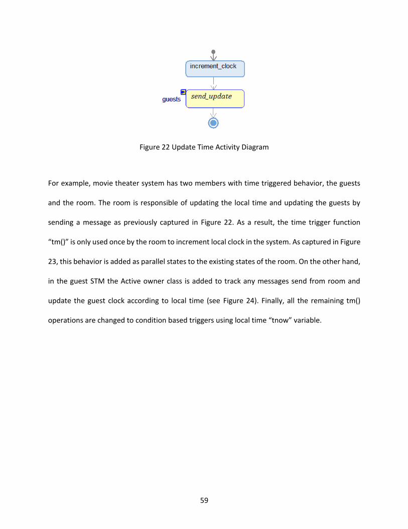
59
Figure 22 Update Time Activity Diagram
For example, movie theater system has two members with time triggered behavior, the guests
and the room. The room is responsible of updating the local time and updating the guests by
sending a message as previously captured in Figure 22. As a result, the time trigger function
“tm()” is only used once by the room to increment local clock in the system. As captured in Figure
23, this behavior is added as parallel states to the existing states of the room. On the other hand,
in the guest STM the Active owner class is added to track any messages send from room and
update the guest clock according to local time (see Figure 24). Finally, all the remaining tm()
operations are changed to condition based triggers using local time “tnow” variable.

60
Figure 23 Room State Diagram
Additional to fixing synchronization issues, separation of this behavior can support modeling
efforts with two main areas. First, if designed models are to be exported to a different simulation
software, system behavior can be separated and exported explicitly. Furthermore, update time
can also be exported explicitly to be used in modeling other systems. Rhapsody specific behavior
such as “update_time” or “generate_variate” can be allocated to a unique system component or
grouped under Location.
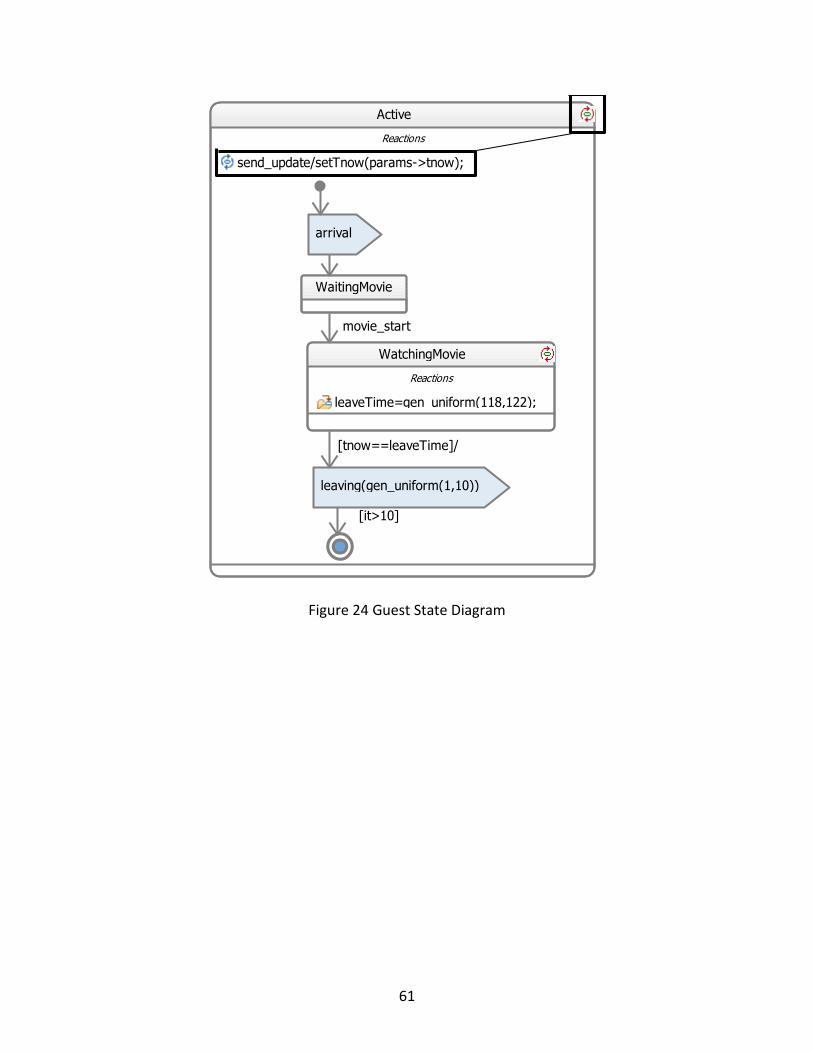
61
Figure 24 Guest State Diagram
Active
Reactions
send_update/setTnow(params->tnow);
WatchingMovie
Reactions
leaveTime=gen_uniform(118,122);
leaving(gen_uniform(1,10)) to proom
[tnow==leaveTime]/FILE * pFile; pFile = fopen ("results.txt","a+"); fprintf(pFile, "Iteration %d %d\n",it,leaveTime);fclose (pFile);printf("%d %d\n",tnow,leaveTime)
WaitingMovie
movie_start
arrival to proom
[it>10]

62
CHAPTER FIVE: POPULATION DYNAMICS CASE STUDY
This sections uses a hypothetical case study to demonstrate the approach for developing and
simulating an AB-SD hybrid model of a selected system using SysML. Wild life has been a
commonly studied area in AB modeling (Akbas et al., 2015). Therefore, a hypothetical example is
created to demonstrate the methodology focusing on the status of giraffe population in Africa
over time. Five facts (GCF, 2014) and two assumptions about giraffes are selected to describe
specific procedures under different conditions.
Leopard, lion, and hyena are among their predators.
60, 8 and 3% of calves are killed during their first, second and third year, respectively.
Females mature at age 4 and gestation and nursing lasts for 57 to 65 and 4 to 52 weeks,
respectively.
Males start propagating after 7 years old.
Average life span is 25 years.
Assumed ratios for bull to cow and adults to calves are 1 to 1 and 10 to 1, respectively.
Requirements Analysis
According to the 5 requirement groups identified in Methodology chapter, all except first and
last conditions listed above are grouped under behavioral requirements and the remaining two

63
are grouped under structural. On the other hand, the output of interest -status of population-
would be added to the output requirements. A screenshot from Rhapsody® model tree capturing
these requirements and their groups are shown in Figure 25.
Figure 25 Giraffe Population Scenario Requirements
Define Behavior
The behavior of the giraffe population observation system is modeled in seven steps. It starts
with Use Case Diagram (UCD) design and demonstrates the process flows within the developed
approach.
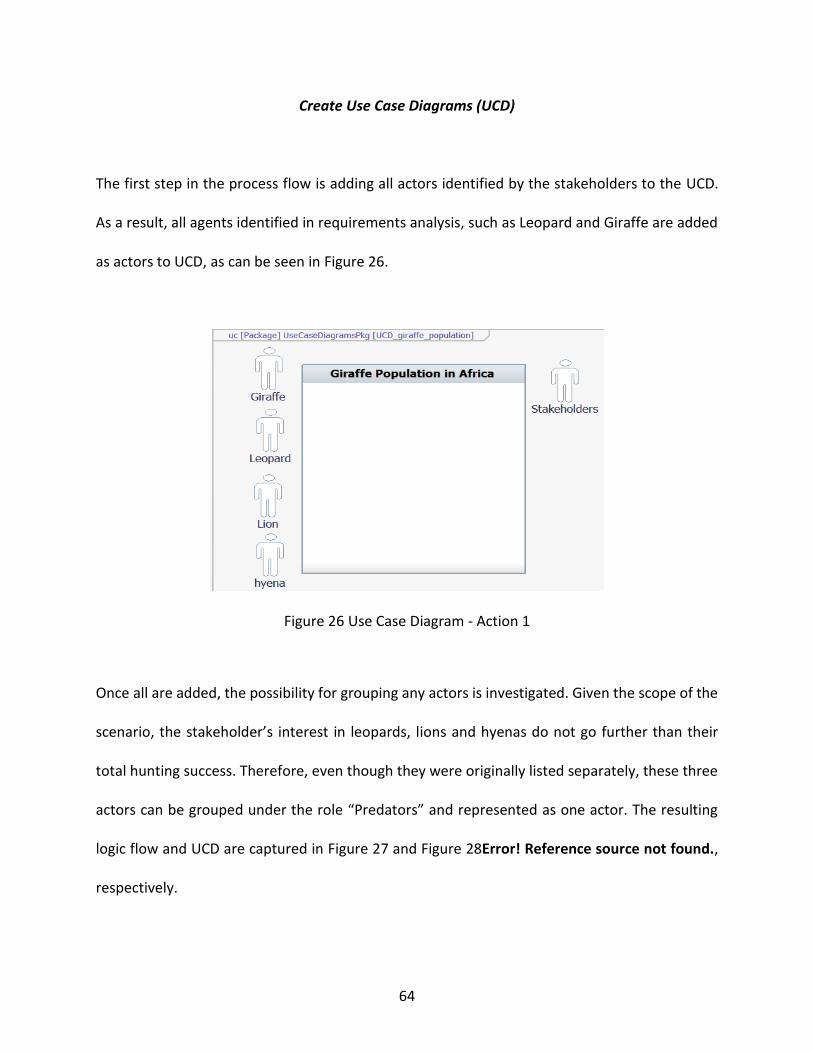
64
Create Use Case Diagrams (UCD)
The first step in the process flow is adding all actors identified by the stakeholders to the UCD.
As a result, all agents identified in requirements analysis, such as Leopard and Giraffe are added
as actors to UCD, as can be seen in Figure 26.
Figure 26 Use Case Diagram - Action 1
Once all are added, the possibility for grouping any actors is investigated. Given the scope of the
scenario, the stakeholder’s interest in leopards, lions and hyenas do not go further than their
total hunting success. Therefore, even though they were originally listed separately, these three
actors can be grouped under the role “Predators” and represented as one actor. The resulting
logic flow and UCD are captured in Figure 27 and Figure 28Error! Reference source not found.,
respectively.
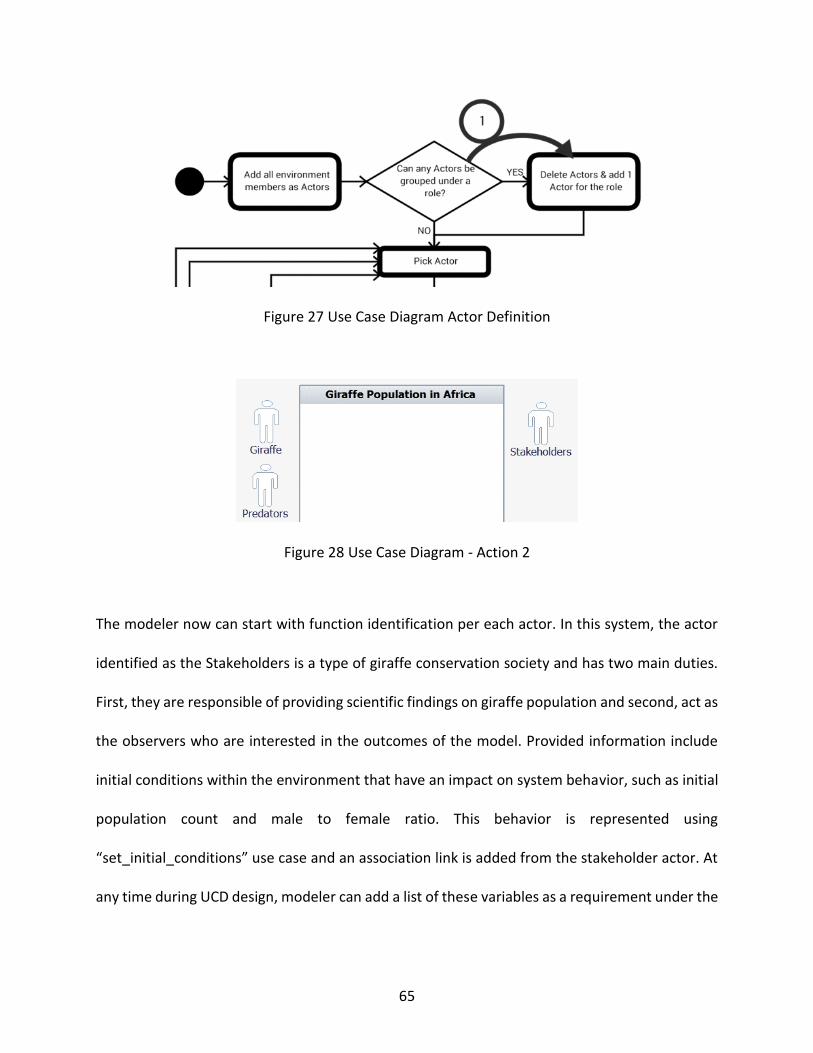
65
Figure 27 Use Case Diagram Actor Definition
Figure 28 Use Case Diagram - Action 2
The modeler now can start with function identification per each actor. In this system, the actor
identified as the Stakeholders is a type of giraffe conservation society and has two main duties.
First, they are responsible of providing scientific findings on giraffe population and second, act as
the observers who are interested in the outcomes of the model. Provided information include
initial conditions within the environment that have an impact on system behavior, such as initial
population count and male to female ratio. This behavior is represented using
“set_initial_conditions” use case and an association link is added from the stakeholder actor. At
any time during UCD design, modeler can add a list of these variables as a requirement under the
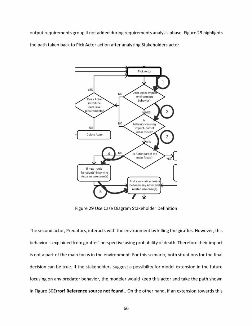
66
output requirements group if not added during requirements analysis phase. Figure 29 highlights
the path taken back to Pick Actor action after analyzing Stakeholders actor.
Figure 29 Use Case Diagram Stakeholder Definition
The second actor, Predators, interacts with the environment by killing the giraffes. However, this
behavior is explained from giraffes’ perspective using probability of death. Therefore their impact
is not a part of the main focus in the environment. For this scenario, both situations for the final
decision can be true. If the stakeholders suggest a possibility for model extension in the future
focusing on any predator behavior, the modeler would keep this actor and take the path shown
in Figure 30Error! Reference source not found.. On the other hand, if an extension towards this

67
direction is not within stakeholder interests, this actor can be deleted. It is important to note
that, this should only be considered if no interaction exists between the selected actor and any
member of the environment.
Figure 30 Use Case Diagram Predator Definition
The final actor Giraffe is a part of the main environment scope, therefore is not included as an
external member in the UCD. Later in architectural design this will be added as a part of the
system structure. Provided assumptions suggest two functions, “reproduce“ and “die” and no
information is given about the effect of their location information nor is included within
environment interests. Reproduce is defined as a duration triggered function and die is defined
as a success rate changing over time. Since the time is used by more than one a use case named
“update_time” is added to keep the behavior synchronized. This is further explained in Time
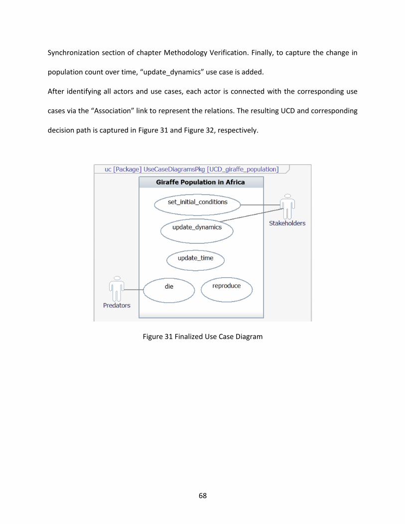
68
Synchronization section of chapter Methodology Verification. Finally, to capture the change in
population count over time, “update_dynamics” use case is added.
After identifying all actors and use cases, each actor is connected with the corresponding use
cases via the “Association” link to represent the relations. The resulting UCD and corresponding
decision path is captured in Figure 31 and Figure 32, respectively.
Figure 31 Finalized Use Case Diagram
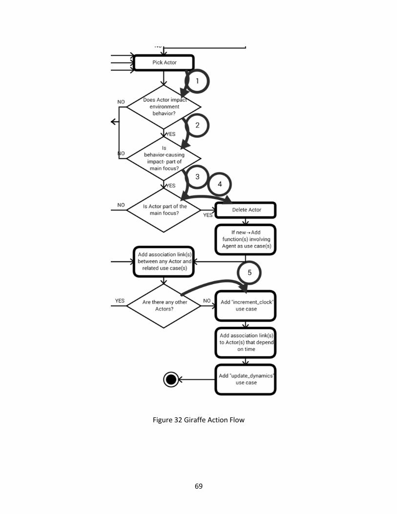
69
Figure 32 Giraffe Action Flow
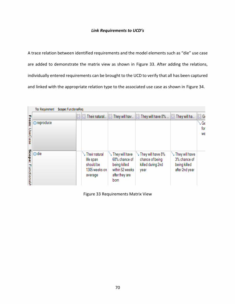
70
Link Requirements to UCD’s
A trace relation between identified requirements and the model elements such as “die” use case
are added to demonstrate the matrix view as shown in Figure 33. After adding the relations,
individually entered requirements can be brought to the UCD to verify that all has been captured
and linked with the appropriate relation type to the associated use case as shown in Figure 34.
Figure 33 Requirements Matrix View

71
Figure 34 Finalized Use Case Diagram

72
Create Activity Diagrams (ActD)
The ActD for system specific use cases includes the actions belonging to “reproduce” and “die”
behaviors as captured in Figure 35 and Figure 36 simultaneously. According to system
description, pregnancy lasts between 57 to 65 weeks after propagation. To capture this duration
“pregnancy_duration” and “pregnancy_status” variables are added to the reproduce behavior
block.
Figure 35 Reproduce Activity Diagram
There are four conditions that result in the death of a giraffe. Three of them are their chance of
survival after a predator attack. If they survive all, they will die at the end of their natural life
span. To capture this behavior, four variables, “age”, “survival_chance”, “survival_duration” and
“life_span” are added. If the modeler is using Rhapsody with the Harmony Profile, embedded
code for each action can be added during state definition phase.
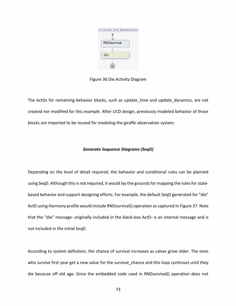
73
Figure 36 Die Activity Diagram
The ActDs for remaining behavior blocks, such as update_time and update_dynamics, are not
created nor modified for this example. After UCD design, previously modeled behavior of those
blocks are imported to be reused for modeling the giraffe observation system.
Generate Sequence Diagrams (SeqD)
Depending on the level of detail required, the behavior and conditional rules can be planned
using SeqD. Although this is not required, it would lay the grounds for mapping the rules for state-
based behavior and support designing efforts. For example, the default SeqD generated for “die”
ActD using Harmony profile would include RNDsurvival() operation as captured in Figure 37. Note
that the “die” message- originally included in the black-box ActD- is an internal message and is
not included in the initial SeqD.
According to system definition, the chance of survival increases as calves grow older. The ones
who survive first year get a new value for the survival_chance and this loop continues until they
die because off old age. Since the embedded code used in RNDsurvival() operation does not
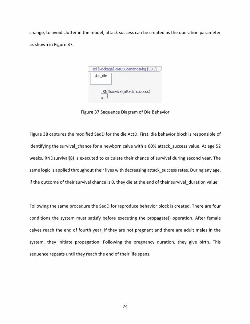
74
change, to avoid clutter in the model, attack success can be created as the operation parameter
as shown in Figure 37.
Figure 37 Sequence Diagram of Die Behavior
Figure 38 captures the modified SeqD for the die ActD. First, die behavior block is responsible of
identifying the survival_chance for a newborn calve with a 60% attack_success value. At age 52
weeks, RNDsurvival(8) is executed to calculate their chance of survival during second year. The
same logic is applied throughout their lives with decreasing attack_success rates. During any age,
if the outcome of their survival chance is 0, they die at the end of their survival_duration value.
Following the same procedure the SeqD for reproduce behavior block is created. There are four
conditions the system must satisfy before executing the propagate() operation. After female
calves reach the end of fourth year, if they are not pregnant and there are adult males in the
system, they initiate propagation. Following the pregnancy duration, they give birth. This
sequence repeats until they reach the end of their life spans.
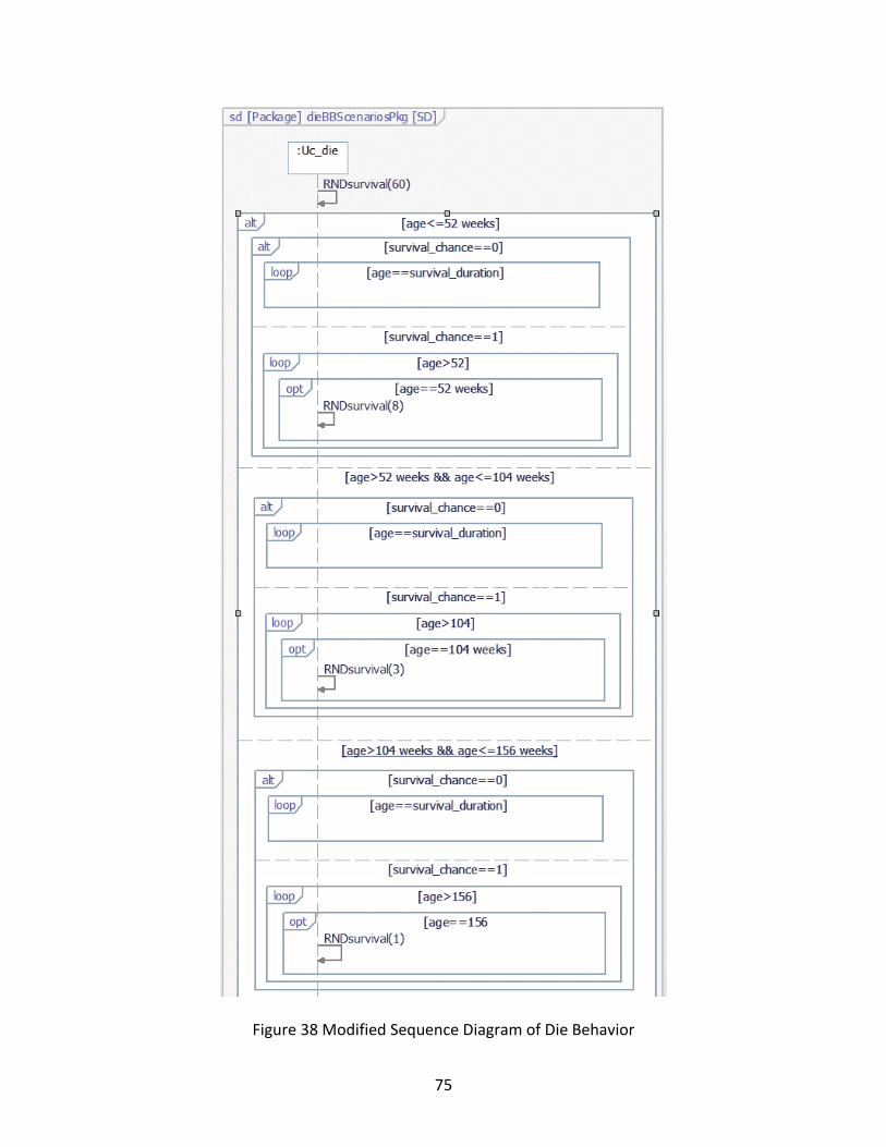
75
Figure 38 Modified Sequence Diagram of Die Behavior
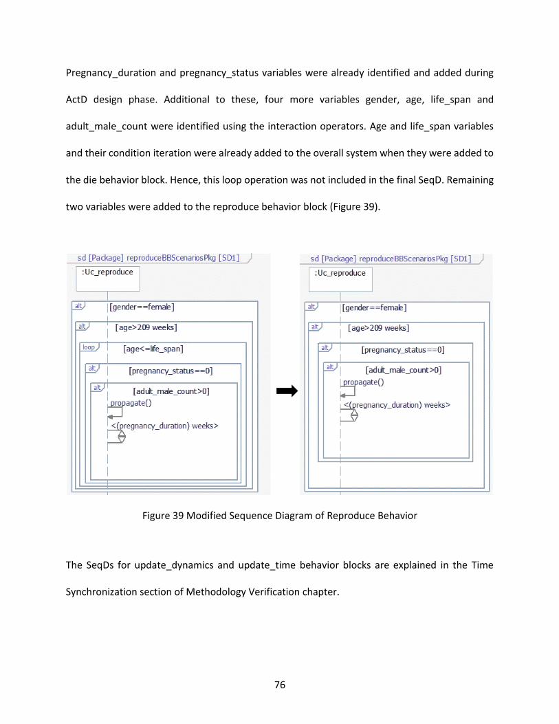
76
Pregnancy_duration and pregnancy_status variables were already identified and added during
ActD design phase. Additional to these, four more variables gender, age, life_span and
adult_male_count were identified using the interaction operators. Age and life_span variables
and their condition iteration were already added to the overall system when they were added to
the die behavior block. Hence, this loop operation was not included in the final SeqD. Remaining
two variables were added to the reproduce behavior block (Figure 39).
Figure 39 Modified Sequence Diagram of Reproduce Behavior
The SeqDs for update_dynamics and update_time behavior blocks are explained in the Time
Synchronization section of Methodology Verification chapter.
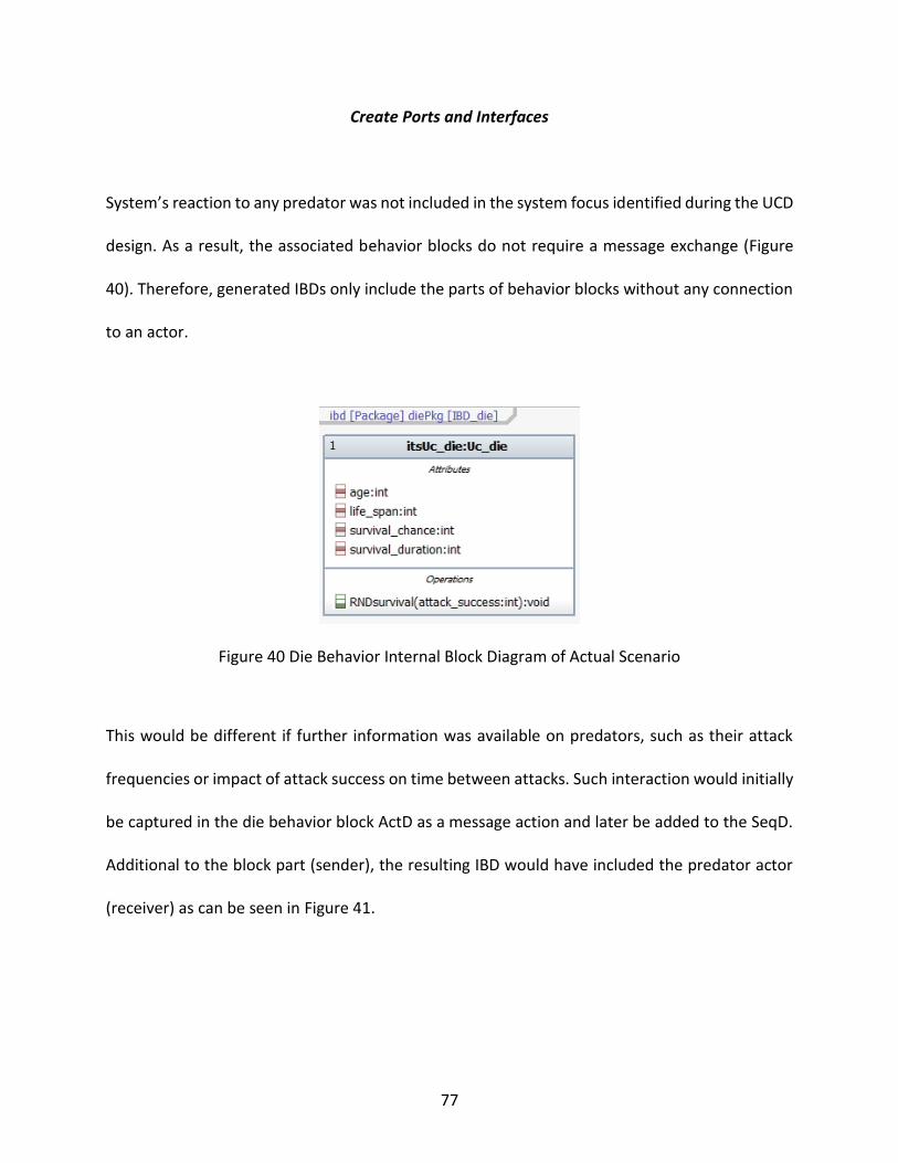
77
Create Ports and Interfaces
System’s reaction to any predator was not included in the system focus identified during the UCD
design. As a result, the associated behavior blocks do not require a message exchange (Figure
40). Therefore, generated IBDs only include the parts of behavior blocks without any connection
to an actor.
Figure 40 Die Behavior Internal Block Diagram of Actual Scenario
This would be different if further information was available on predators, such as their attack
frequencies or impact of attack success on time between attacks. Such interaction would initially
be captured in the die behavior block ActD as a message action and later be added to the SeqD.
Additional to the block part (sender), the resulting IBD would have included the predator actor
(receiver) as can be seen in Figure 41.
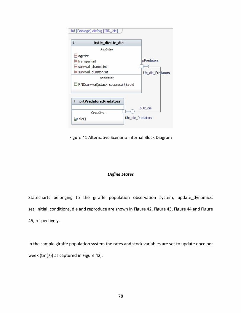
78
Figure 41 Alternative Scenario Internal Block Diagram
Define States
Statecharts belonging to the giraffe population observation system, update_dynamics,
set_initial_conditions, die and reproduce are shown in Figure 42, Figure 43, Figure 44 and Figure
45, respectively.
In the sample giraffe population system the rates and stock variables are set to update once per
week (tm(7)) as captured in Figure 42,.
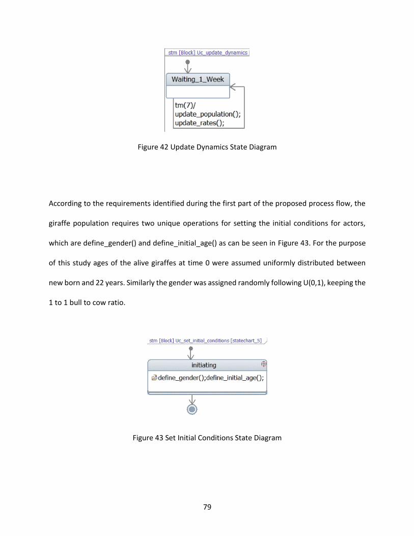
79
Figure 42 Update Dynamics State Diagram
According to the requirements identified during the first part of the proposed process flow, the
giraffe population requires two unique operations for setting the initial conditions for actors,
which are define_gender() and define_initial_age() as can be seen in Figure 43. For the purpose
of this study ages of the alive giraffes at time 0 were assumed uniformly distributed between
new born and 22 years. Similarly the gender was assigned randomly following U(0,1), keeping the
1 to 1 bull to cow ratio.
Figure 43 Set Initial Conditions State Diagram
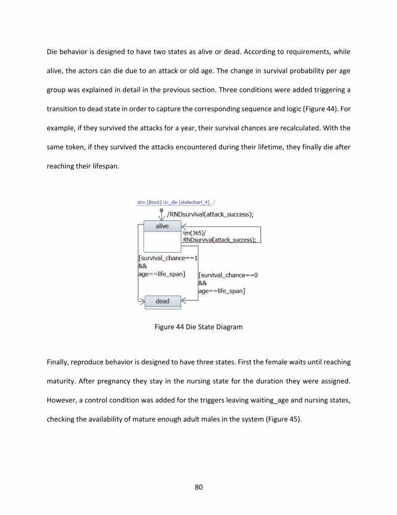
80
Die behavior is designed to have two states as alive or dead. According to requirements, while
alive, the actors can die due to an attack or old age. The change in survival probability per age
group was explained in detail in the previous section. Three conditions were added triggering a
transition to dead state in order to capture the corresponding sequence and logic (Figure 44). For
example, if they survived the attacks for a year, their survival chances are recalculated. With the
same token, if they survived the attacks encountered during their lifetime, they finally die after
reaching their lifespan.
Figure 44 Die State Diagram
Finally, reproduce behavior is designed to have three states. First the female waits until reaching
maturity. After pregnancy they stay in the nursing state for the duration they were assigned.
However, a control condition was added for the triggers leaving waiting_age and nursing states,
checking the availability of mature enough adult males in the system (Figure 45).
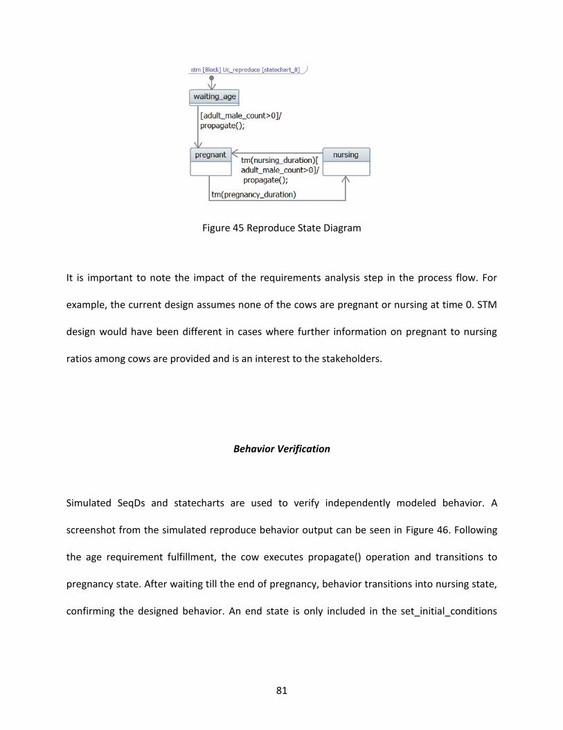
81
Figure 45 Reproduce State Diagram
It is important to note the impact of the requirements analysis step in the process flow. For
example, the current design assumes none of the cows are pregnant or nursing at time 0. STM
design would have been different in cases where further information on pregnant to nursing
ratios among cows are provided and is an interest to the stakeholders.
Behavior Verification
Simulated SeqDs and statecharts are used to verify independently modeled behavior. A
screenshot from the simulated reproduce behavior output can be seen in Figure 46. Following
the age requirement fulfillment, the cow executes propagate() operation and transitions to
pregnancy state. After waiting till the end of pregnancy, behavior transitions into nursing state,
confirming the designed behavior. An end state is only included in the set_initial_conditions
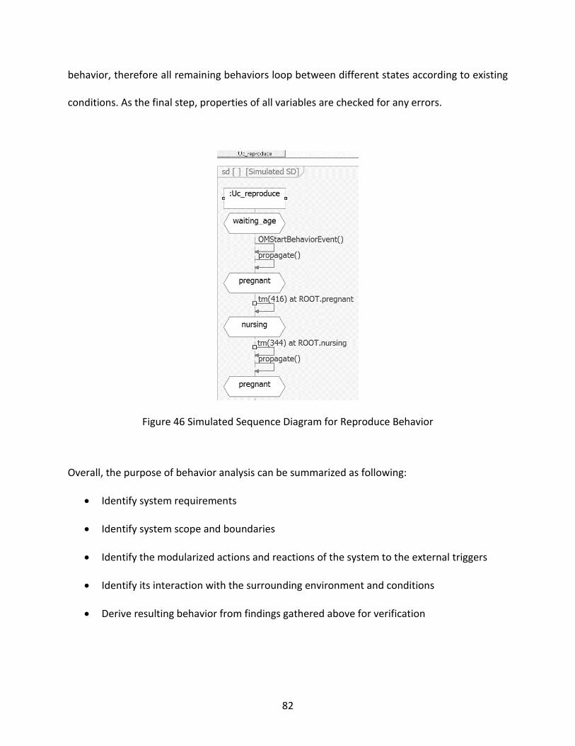
82
behavior, therefore all remaining behaviors loop between different states according to existing
conditions. As the final step, properties of all variables are checked for any errors.
Figure 46 Simulated Sequence Diagram for Reproduce Behavior
Overall, the purpose of behavior analysis can be summarized as following:
Identify system requirements
Identify system scope and boundaries
Identify the modularized actions and reactions of the system to the external triggers
Identify its interaction with the surrounding environment and conditions
Derive resulting behavior from findings gathered above for verification

83
Define Structure
Structure modeling starts with decomposing the system according to its physical components
using Block Definition Diagrams. Later previously modeled independent behavior is merged and
distributed to the responsible part of the system.
Create Block Definition Diagrams
Giraffe population observation system is decomposed using Type III decomposition structure due
to the two way dependency between the giraffes and their location. Initially eighty giraffes are
created sharing one location, Africa, as can be seen in Figure 47.
Figure 47 Block Definition Diagram
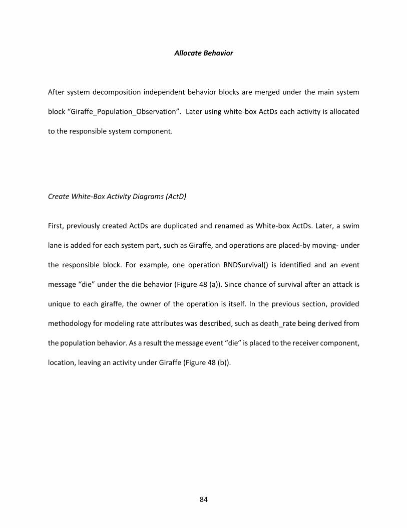
84
Allocate Behavior
After system decomposition independent behavior blocks are merged under the main system
block “Giraffe_Population_Observation”. Later using white-box ActDs each activity is allocated
to the responsible system component.
Create White-Box Activity Diagrams (ActD)
First, previously created ActDs are duplicated and renamed as White-box ActDs. Later, a swim
lane is added for each system part, such as Giraffe, and operations are placed-by moving- under
the responsible block. For example, one operation RNDSurvival() is identified and an event
message “die” under the die behavior (Figure 48 (a)). Since chance of survival after an attack is
unique to each giraffe, the owner of the operation is itself. In the previous section, provided
methodology for modeling rate attributes was described, such as death_rate being derived from
the population behavior. As a result the message event “die” is placed to the receiver component,
location, leaving an activity under Giraffe (Figure 48 (b)).
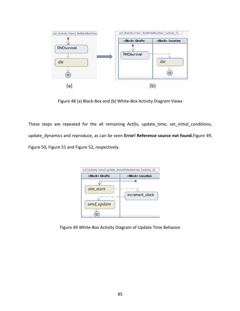
85
Figure 48 (a) Black-Box and (b) White-Box Activity Diagram Views
These steps are repeated for the all remaining ActDs, update_time, set_initial_conditions,
update_dynamics and reproduce, as can be seen Error! Reference source not found.Figure 49,
Figure 50, Figure 51 and Figure 52, respectively.
Figure 49 White-Box Activity Diagram of Update Time Behavior
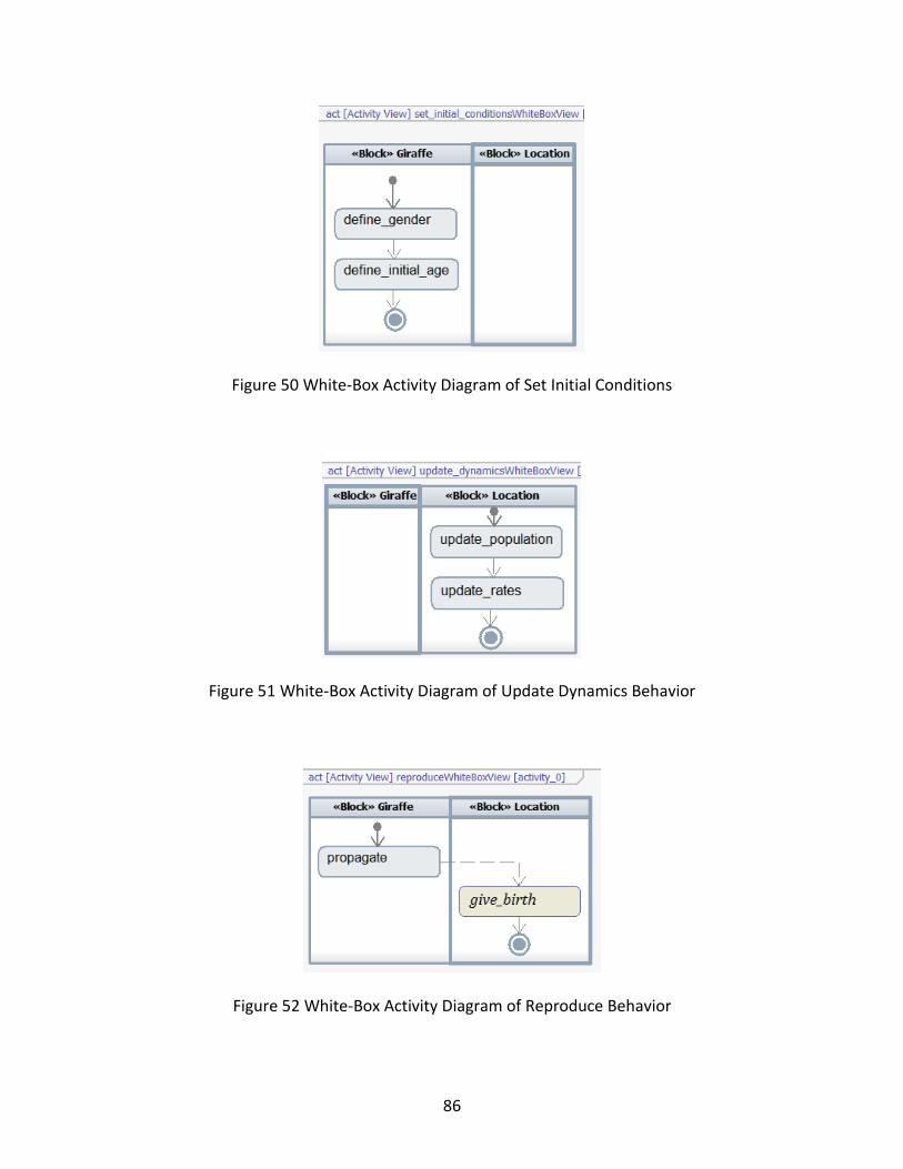
86
Figure 50 White-Box Activity Diagram of Set Initial Conditions
Figure 51 White-Box Activity Diagram of Update Dynamics Behavior
Figure 52 White-Box Activity Diagram of Reproduce Behavior

87
Generate Sequence Diagrams (SeqD) and Create Ports and Interfaces
After each behavior is allocated to the responsible part of the system Harmony profile is used for
generating the SeqDs and for creating the ports and event interfaces.
Define States
Location part of the system is responsible of executing two behaviors. After starting the
simulation it transitions to an “Active” state where it performs Update_time and
update_dynamics behaviors, which are integrated as and-states. Update_dynamics is responsible
of updating the population variable and the weekly rates on the seventh day every week (Figure
53).
Figure 53 Location State Diagram
88
The behaviors of giraffes are activated when the simulation clock starts running at the location.
The initially deployed giraffes, who are assumed to be already in the environment, are assigned
a random gender, age and survival_chance (based on the initial age group) to represent a
uniformly distributed population. Furthermore, gender of a calf born after time 0 is randomly
selected based on the cow to bull proportions within the population. This logic is designed to
satisfy the ratio requirement identified in problem description.
Contradictory to using “and-states”, such-as in Figure 53, the reproduce behavior was added as
a subset to being alive (see Figure 54). Later, alive state was further divided into two “and-states”
and the top portion was used to show the gender of a giraffe after maturity to demonstrate
simulated view when in parallel states.
Verify and Validate System
Three tests are conducted to validate the behavior designed for Giraffe Population Observation
System. First the model is verified using the simulated SeqD and statecharts. Later, results from
30 simulation iterations are collected using an initial population size of 140 giraffes for the second
and third tests. Three values at any given time t in days for population count, births and deaths
per week, are collected and their averages are plotted in Figure 55Error! Reference source not
found.. Two expected behaviors are tested as follows:
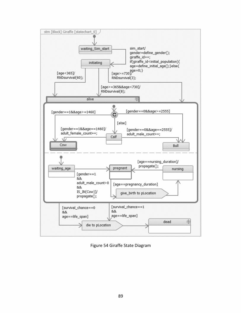
89
Figure 54 Giraffe State Diagram
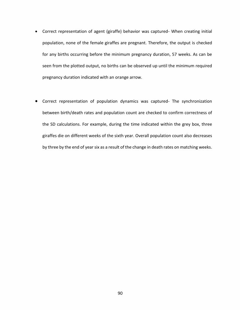
90
Correct representation of agent (giraffe) behavior was captured- When creating initial
population, none of the female giraffes are pregnant. Therefore, the output is checked
for any births occurring before the minimum pregnancy duration, 57 weeks. As can be
seen from the plotted output, no births can be observed up until the minimum required
pregnancy duration indicated with an orange arrow.
Correct representation of population dynamics was captured- The synchronization
between birth/death rates and population count are checked to confirm correctness of
the SD calculations. For example, during the time indicated within the grey box, three
giraffes die on different weeks of the sixth year. Overall population count also decreases
by three by the end of year six as a result of the change in death rates on matching weeks.
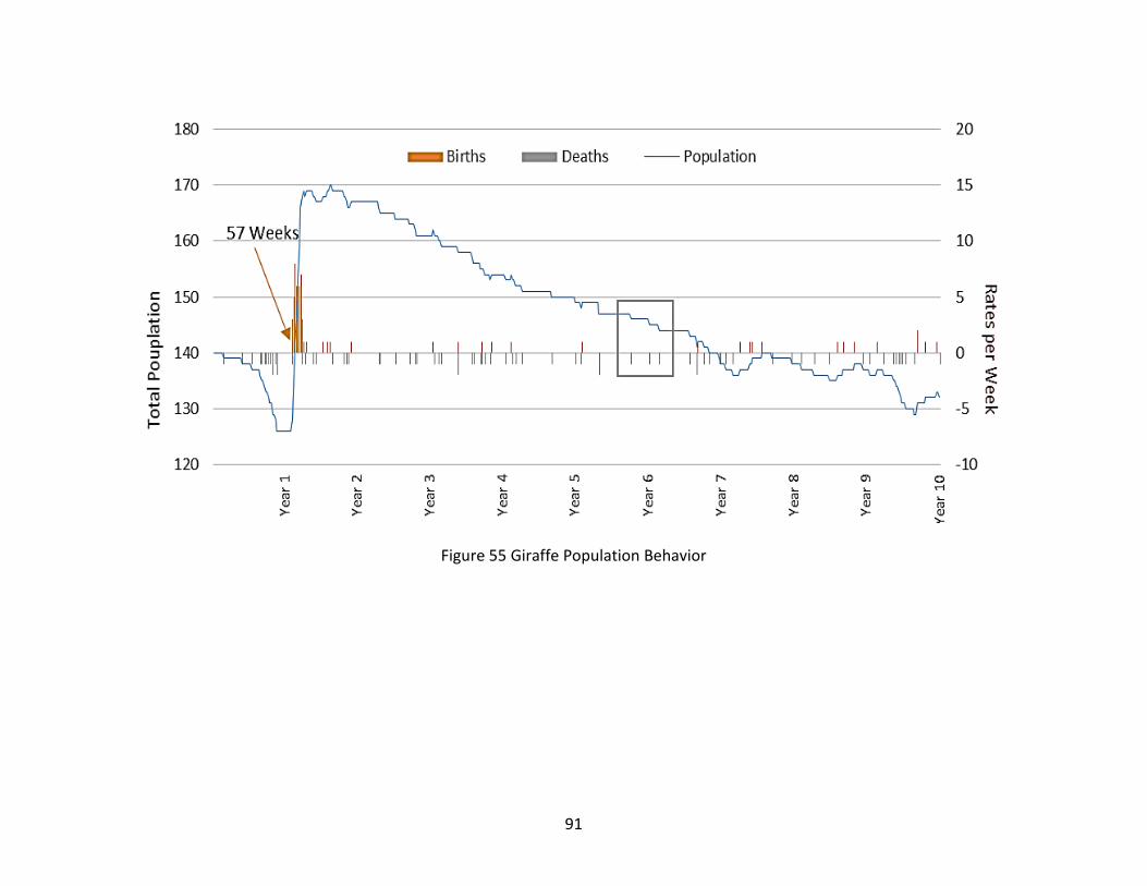
91
Figure 55 Giraffe Population Behavior

92
CHAPTER SIX: TRAINING MANAGEMENT CASE STUDY
In this section the application of the developed approach is demonstrated using a real-life case
study focusing on a training management project which was planned and executed when a large-
scale company had decided to adapt a new software technology in 2009. The project required
1255 employees’ attendance from different divisions and backgrounds. This new technology was
the same as to what engineers had already been using; however, the processes were changed.
When they were used to working on locally saved files, and sharing these documents mostly using
emails, employees were asked to do all using this new technology. In addition to the extra work
created by the efforts spent on a new technology, each employee was asked to attend an eight-
hour (full-day) training. At the end of four fiscal years (FY), in 2012, only 1007 employees out of
1255 were trained where the total training capacity was over 2300 seats (Figure 56).
Furthermore, by 2011, more than 29% of trained were returning for a second training. Obtained
data included versions of a Microsoft Excel sheet saved at different times over the project
duration, created for attendance tracking. The purpose of the modeling effort focusses on
supporting project management team by simulating the training bubble to be used for training
scheduling.
93
Figure 56 Total Training Attendance
Training Management as Complex Adaptive Systems
Two characteristics that are most commonly observed in complex systems are emergence of a
pattern and continual appearance of new entity kinds (Levin, 2002) or large number of interacting
entities (Morel and Ramajujam, 1999). Emergence was explained as being dynamic behavior of
balanced negative and positive feedback rather than being the absence of tension (Newell, 2008).
Because of the variety in forms of complexity, one cannot conclude that all complex systems are
adaptive (Levin, 2002). Furthermore, complexity in systems cannot be explained by chaos (Bak,
1996, p. 31), meaning systems with simple dynamics can be very complex thus they do not have
to be chaotic to be accepted complex (Morel and Ramanujam, 1999).
94
The existence of complexity in learning systems, a phrase introduced by Davis and Simmt (2003)
describing collective classroom components, is advocated by also other researchers (Burns and
Knox, 2011, Davis and Sumara, 2006). Newell (2008), following Davis, Simmt and Sumara’s
published arguments on how individual learner and teacher dynamics interacts and emerges as
learning, evaluates the potential benefits and challenges of accepting this theory.
Unlike immediate training climate, studies on organizations as systems has a longer history, and
today, they are accepted as “dynamic systems of adaptation and evolution that contain multiple
parts which interact with one another and the environment” (Morel and Ramanujam, 1999).
Furthermore, their nested structure continuously interacts with other macro and micro, systems
and sub-systems, respectively (Folke & Folke, 1992). New systems may arise from emerging
dynamics as part of the system, due to change processes occurring with an organization (Dooley
and Van de Ven, 1999). Bot (2012) has listed the most common properties of complex systems in
a study where he looked into the complexity of learning a third language. Training management
was evaluated with respect to each property listed by Bot, and the findings were captured in
Table 3. Explanations and case examples were supported with findings from literature. The
findings support the theory of training management emerged as complex adaptive-derived from
its evolution through a life-cycle iterations-system that interacts with other complex adaptive
systems such as technology and economy.

95
Table 3 Complex System Properties, Adapted from Bot, 2012
Complex System Properties Training Management System Properties
Complex systems are sets of interacting variables. Training management interacts with organization system (macro) and knowledge transfer variables (micro).
In many complex systems, the outcome of development over time cannot be predicted … because the variables that interact keep changing over time.
Although there are techniques to support training planning often times changes in duration, cost, training performance occur.
Dynamic systems are always part of another system, going from sub-molecular particles to the universe.
Training management system is part of knowledge transfer system.
As they develop over time, dynamic subsystems appear to settle in specific states, which are preferred but unpredictable, so-called ‘attractor states.’
Employees within an organization create a unique knowledge share structure creating a culture which emerges individual and organization’s learning state. Weick (1979)
Systems develop through iterations of simple procedures that are applied over and over again, with the output of the preceding iteration as the input of the next.
Training is applied in organizations in iterations, the lessons learned from each experience (outputs) feeds the following management strategy as inputs. (Armstrong, 2003)
The development of a dynamic system appears to be highly dependent on its beginning state. Minor differences at the beginning can have dramatic consequences in the long run. …
If started without well planning the effects of each variable and their interactions, training efforts will fail costing the investments and time of the stakeholders.
In dynamic systems, changes in one variable have an impact on all other variables that are part of the system: systems are fully interconnected.
In training management, change in one variable for instance organization’s climate or available resources will trigger a change in the whole system will affect outcomes.
In natural systems, development is dependent on resources: … all natural systems will tend to entropy when no additional energy is added to the system.
Training management rely on the resource availability, depletion of any resource will trigger system’s state to change to ‘steady-state’.
Systems develop through interaction with their environment and through internal self-reorganization.
Training has emerged from interaction of systems such as learning, organization and technology. Through time its internal interactions derived management variables (Dooley and Van de Ven, 1999)
Because systems are constantly in flow, they will show variation, which makes them sensitive to specific input at a given point in time and some other input at another point in time.
Due to continuous change in it is variables such as humans and technology same management approaches will result in varying outputs.

96
Model Development
Structural and behavioral characteristics of the systems, such as input analysis, are identified first,
through requirements analysis. Later identified behavior is individually modeled under behavior
analysis. After verification, the behavior is integrated and allocated to parts of the system in
structure analysis. Finally, the model is verified and validated and the findings are discussed.
Requirements Analysis
The majority of the work completed in this phase consists of input analysis. Each of the original
training status report snapshots included training dates of ranging from 3,000 to 10,000
employees, which also consisted of contradicting or duplicate information. First, using the latest
report, a skeleton list including the generated id’s of employees located in US, who had either
attended training or was required to attend in the future is generated. Later all ID’s in each
snapshot that were not included in this list are deleted. Each duplicate id is deleted after
confirming all attendance data are successfully copied in to the remaining. Due to the length of
the project, some sessions had been renamed over the years, and to avoid double-counting, a
total of 13,173 data points are checked individually for potential duplicate attendance
information. Using the data population increase, training attendance, attendance probability and
training schedule are studied as further explained respectively in the following sections.
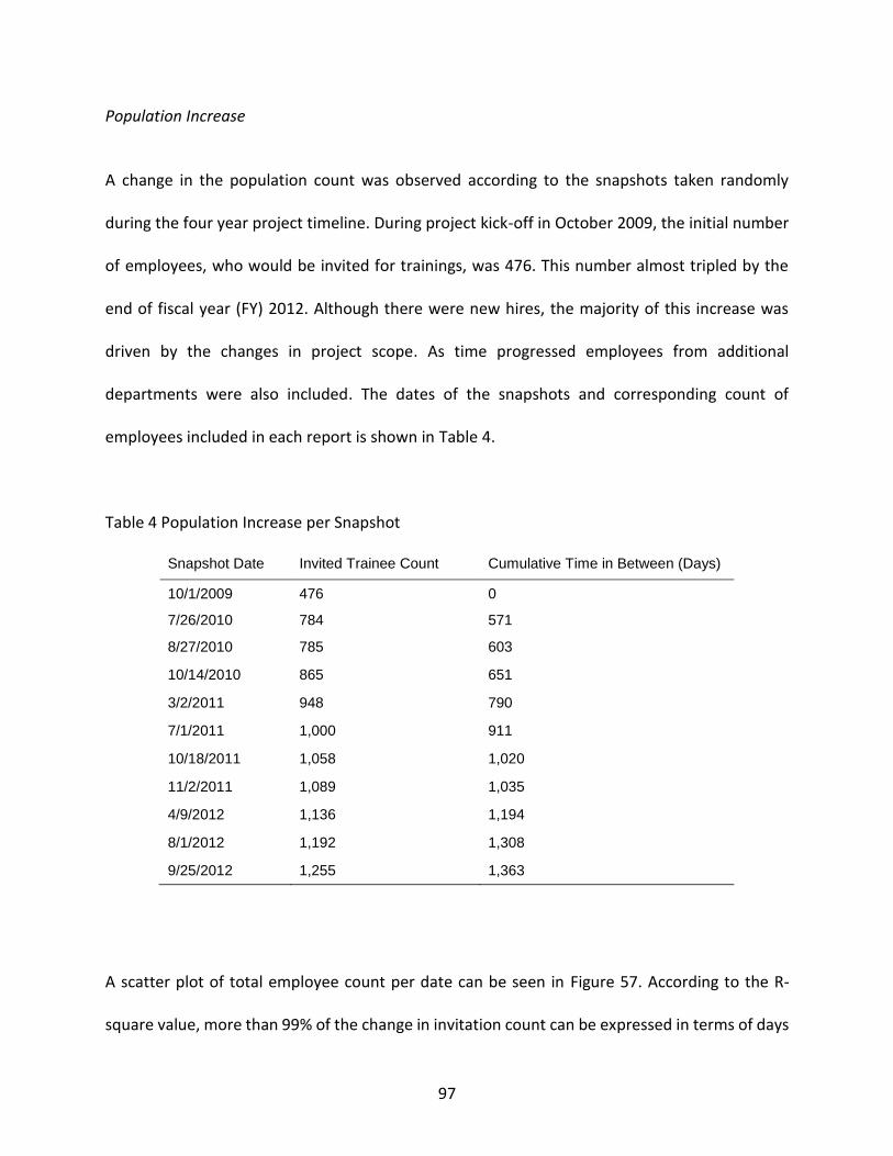
97
Population Increase
A change in the population count was observed according to the snapshots taken randomly
during the four year project timeline. During project kick-off in October 2009, the initial number
of employees, who would be invited for trainings, was 476. This number almost tripled by the
end of fiscal year (FY) 2012. Although there were new hires, the majority of this increase was
driven by the changes in project scope. As time progressed employees from additional
departments were also included. The dates of the snapshots and corresponding count of
employees included in each report is shown in Table 4.
Table 4 Population Increase per Snapshot
Snapshot Date Invited Trainee Count Cumulative Time in Between (Days)
10/1/2009 476 0
7/26/2010 784 571
8/27/2010 785 603
10/14/2010 865 651
3/2/2011 948 790
7/1/2011 1,000 911
10/18/2011 1,058 1,020
11/2/2011 1,089 1,035
4/9/2012 1,136 1,194
8/1/2012 1,192 1,308
9/25/2012 1,255 1,363
A scatter plot of total employee count per date can be seen in Figure 57. According to the R-
square value, more than 99% of the change in invitation count can be expressed in terms of days
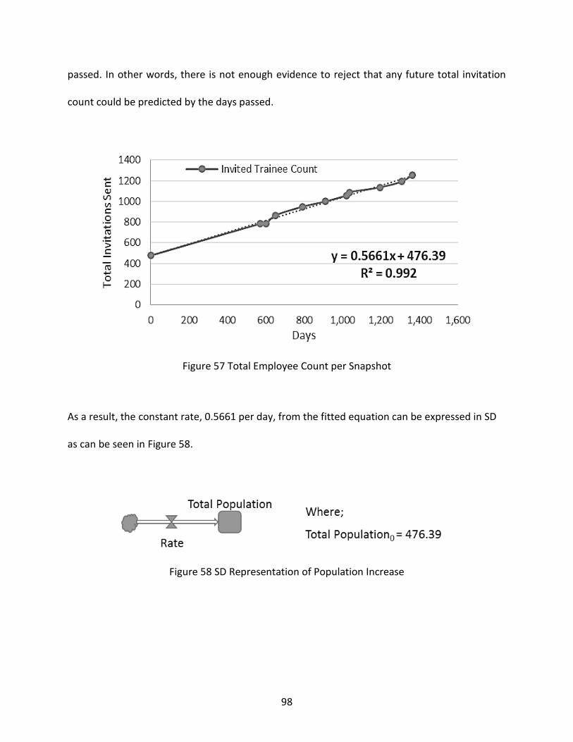
98
passed. In other words, there is not enough evidence to reject that any future total invitation
count could be predicted by the days passed.
Figure 57 Total Employee Count per Snapshot
As a result, the constant rate, 0.5661 per day, from the fitted equation can be expressed in SD
as can be seen in Figure 58.
Figure 58 SD Representation of Population Increase

99
Training Attendance
The first focus in the attendance analysis is the behavior of employees who had attended a
training more than once over the years. However, out of 1255, only eight employees had
attended training three times and none had attended more than that. Due to the limit of this
data and its ratio to the total sample size, the dates from their third attendance is not included
in the study. The date of the first training and the time, in days, until the second training are
mapped and checked for any outliers.
A scatter plot is created to test dependency between the first training date and the time until the
second, Delay, as captured in Figure 59. The total sample size is 124 with a mean and standard
deviation at 436 and 230 days, respectively. The R-Square value, 0.133, of the fitted equation is
not significant enough to reject dependency.
Figure 59 Delay vs Initial Training Date
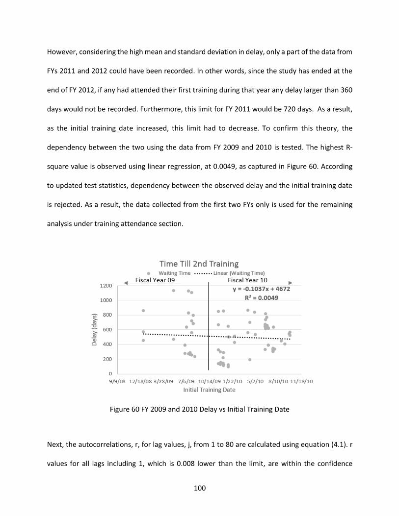
100
However, considering the high mean and standard deviation in delay, only a part of the data from
FYs 2011 and 2012 could have been recorded. In other words, since the study has ended at the
end of FY 2012, if any had attended their first training during that year any delay larger than 360
days would not be recorded. Furthermore, this limit for FY 2011 would be 720 days. As a result,
as the initial training date increased, this limit had to decrease. To confirm this theory, the
dependency between the two using the data from FY 2009 and 2010 is tested. The highest R-
square value is observed using linear regression, at 0.0049, as captured in Figure 60. According
to updated test statistics, dependency between the observed delay and the initial training date
is rejected. As a result, the data collected from the first two FYs only is used for the remaining
analysis under training attendance section.
Figure 60 FY 2009 and 2010 Delay vs Initial Training Date
Next, the autocorrelations, r, for lag values, j, from 1 to 80 are calculated using equation (4.1). r
values for all lags including 1, which is 0.008 lower than the limit, are within the confidence
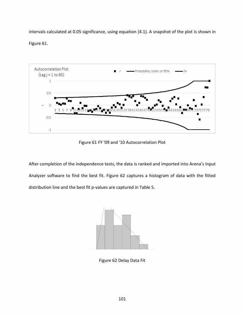
101
intervals calculated at 0.05 significance, using equation (4.1). A snapshot of the plot is shown in
Figure 61.
Figure 61 FY '09 and '10 Autocorrelation Plot
After completion of the independence tests, the data is ranked and imported into Arena’s Input
Analyzer software to find the best fit. Figure 62 captures a histogram of data with the fitted
distribution line and the best fit p-values are captured in Table 5.
Figure 62 Delay Data Fit
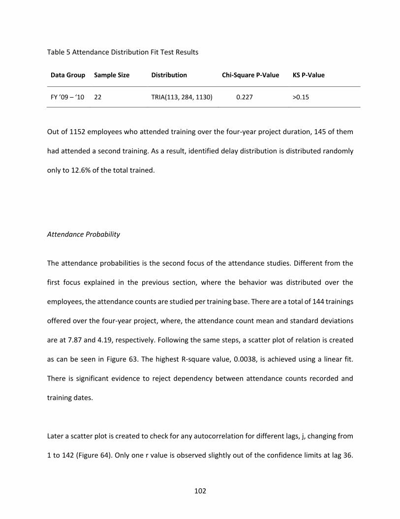
102
Table 5 Attendance Distribution Fit Test Results
Data Group Sample Size Distribution Chi-Square P-Value KS P-Value
FY ’09 – ‘10 22 TRIA(113, 284, 1130) 0.227 >0.15
Out of 1152 employees who attended training over the four-year project duration, 145 of them
had attended a second training. As a result, identified delay distribution is distributed randomly
only to 12.6% of the total trained.
Attendance Probability
The attendance probabilities is the second focus of the attendance studies. Different from the
first focus explained in the previous section, where the behavior was distributed over the
employees, the attendance counts are studied per training base. There are a total of 144 trainings
offered over the four-year project, where, the attendance count mean and standard deviations
are at 7.87 and 4.19, respectively. Following the same steps, a scatter plot of relation is created
as can be seen in Figure 63. The highest R-square value, 0.0038, is achieved using a linear fit.
There is significant evidence to reject dependency between attendance counts recorded and
training dates.
Later a scatter plot is created to check for any autocorrelation for different lags, j, changing from
1 to 142 (Figure 64). Only one r value is observed slightly out of the confidence limits at lag 36.

103
Probability of getting an r value within the confidence limits is therefore 0.993. At 0.05
significance, this suggests enough evidence to reject any autocorrelation.
Figure 63 Attendance Count per Training
Figure 64 Attendance Count Autocorrelation Plot
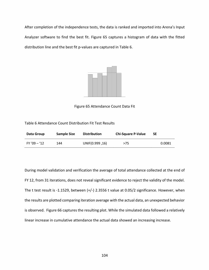
104
After completion of the independence tests, the data is ranked and imported into Arena’s Input
Analyzer software to find the best fit. Figure 65 captures a histogram of data with the fitted
distribution line and the best fit p-values are captured in Table 6.
Figure 65 Attendance Count Data Fit
Table 6 Attendance Count Distribution Fit Test Results
Data Group Sample Size Distribution Chi-Square P-Value SE
FY ’09 – ‘12 144 UNIF(0.999 ,16) >75 0.0081
During model validation and verification the average of total attendance collected at the end of
FY 12, from 31 iterations, does not reveal significant evidence to reject the validity of the model.
The t test result is -1.1529, between (+/-) 2.3556 t value at 0.05/2 significance. However, when
the results are plotted comparing iteration average with the actual data, an unexpected behavior
is observed. Figure 66 captures the resulting plot. While the simulated data followed a relatively
linear increase in cumulative attendance the actual data showed an increasing increase.
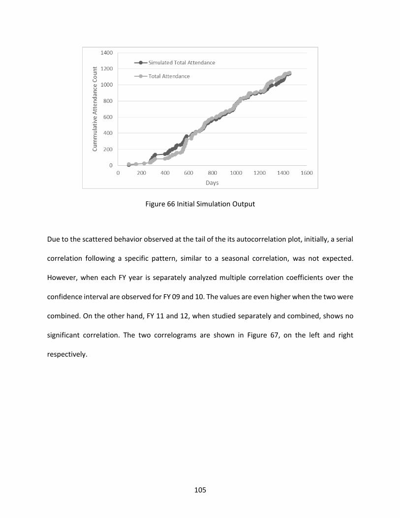
105
Figure 66 Initial Simulation Output
Due to the scattered behavior observed at the tail of the its autocorrelation plot, initially, a serial
correlation following a specific pattern, similar to a seasonal correlation, was not expected.
However, when each FY year is separately analyzed multiple correlation coefficients over the
confidence interval are observed for FY 09 and 10. The values are even higher when the two were
combined. On the other hand, FY 11 and 12, when studied separately and combined, shows no
significant correlation. The two correlograms are shown in Figure 67, on the left and right
respectively.

106
Figure 67 Updated Training Attendance Autocorrelation Plots
FY 09 and 10 are tested for its significance in fitting a time dependent equation, due to failing
independency requirement of data fitting. Highest R-square value, 0.3029 is achieved using an
exponential relation between the time of training and attendance counts per training. Although
R-square value does not find enough evidence to reject the data is a good fit, it is also not enough
to confirm a good fit (The Pennsylvania State University, 2015). The first issue is that R-squared
value displayed is calculated using continuous prediction values. The fitted equation can be used
if the model is SD based only. Since the case model is AB-SD with continuous interaction, a
decimal value would be rounded to the nearest integer, which might result in a lower R-squared.
Hence, the sum of squares (SSR) and total sum of squares are calculated for the rounded values
of predicted attendance (Table 11 in Appendix E).
The new R-squared value calculated from the rounded predictions is found by dividing the sum
of SSR by SSTO. The new fitted equation is y = 1.8206e0.0029x with R-squared at 0.681. Attendance,
rounded predicted attendance and the initial trend line is shown in Figure 68.
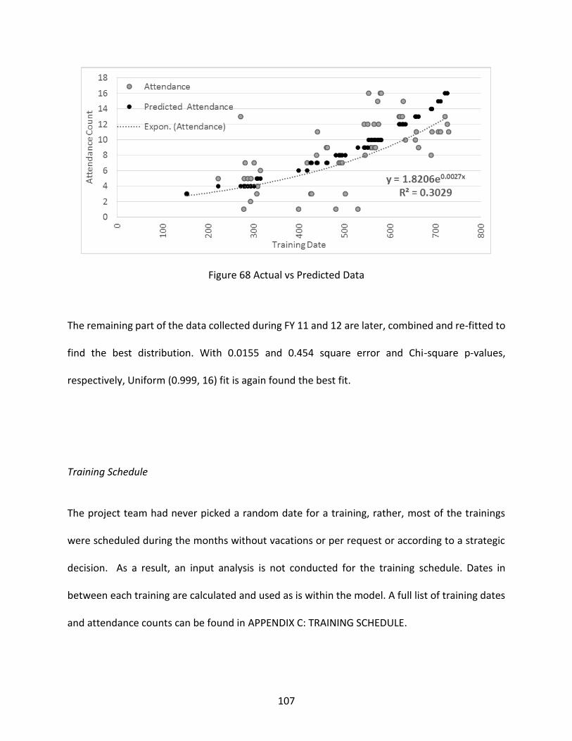
107
Figure 68 Actual vs Predicted Data
The remaining part of the data collected during FY 11 and 12 are later, combined and re-fitted to
find the best distribution. With 0.0155 and 0.454 square error and Chi-square p-values,
respectively, Uniform (0.999, 16) fit is again found the best fit.
Training Schedule
The project team had never picked a random date for a training, rather, most of the trainings
were scheduled during the months without vacations or per request or according to a strategic
decision. As a result, an input analysis is not conducted for the training schedule. Dates in
between each training are calculated and used as is within the model. A full list of training dates
and attendance counts can be found in APPENDIX C: TRAINING SCHEDULE.

108
Define Behavior
The first step in behavior definition is UCD creation. Following the proposed decision flow,
employee agent is removed as an actor, since they are a part of the system scope. Later, their
behavior, “attend_training” is added as a UC. Similarly, the company is also removed as an actor
and its specific behavior “train” is added as a UC. Once all system specific behavior was captured,
pre-modelled common behaviors such as “update_time”, “update_dynamics” and
“set_initial_conditions are imported. The resulting UCD is shown in Figure 69.
Figure 69 Training Management System Usecase Diagram
After identifying the UCs, their relations to requirements are established. Once all functional
requirements are traced back, their black box ActD are designed. First behavior is
“attend_training” whose behavior is based on three conditions. First, class availability is checked
and does not continue with registration unless a seat is available. Second, a decision whether to
show-up to a registered class is made. Finally, re-taking training decision is made. If no-show or
re-take decisions are made, the behavior goes back to the beginning and waits for a seat
availability. This flow is captured in the black-box diagram as shown in Figure 70. The second

109
behavior “train” is responsible of sending invitations and calculating how many employees show-
up at a training (Figure 71).
Figure 70 Attend Training Black-box Activity Diagram
Figure 71 Train Black-box Activity Diagram
The final black-box, set_initial_conditions, is responsible of assigning an employee id to agents
and importing training schedule that is previously identified in the requirements analysis (Figure
72). The remaining two behaviors update_time and update_dynamics use imported ActD that
are previously captured in the Methodology section.
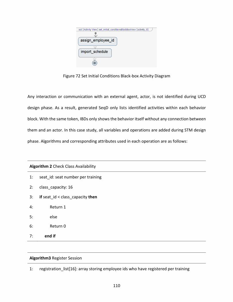
110
Figure 72 Set Initial Conditions Black-box Activity Diagram
Any interaction or communication with an external agent, actor, is not identified during UCD
design phase. As a result, generated SeqD only lists identified activities within each behavior
block. With the same token, IBDs only shows the behavior itself without any connection between
them and an actor. In this case study, all variables and operations are added during STM design
phase. Algorithms and corresponding attributes used in each operation are as follows:
Algorithm 2 Check Class Availability
1: seat_id: seat number per training
2: class_capacity: 16
3: if seat_id < class_capacity then
4: Return 1
5: else
6: Return 0
7: end if
Algorithm3 Register Session
1: registration_list[16]: array storing employee ids who have registered per training
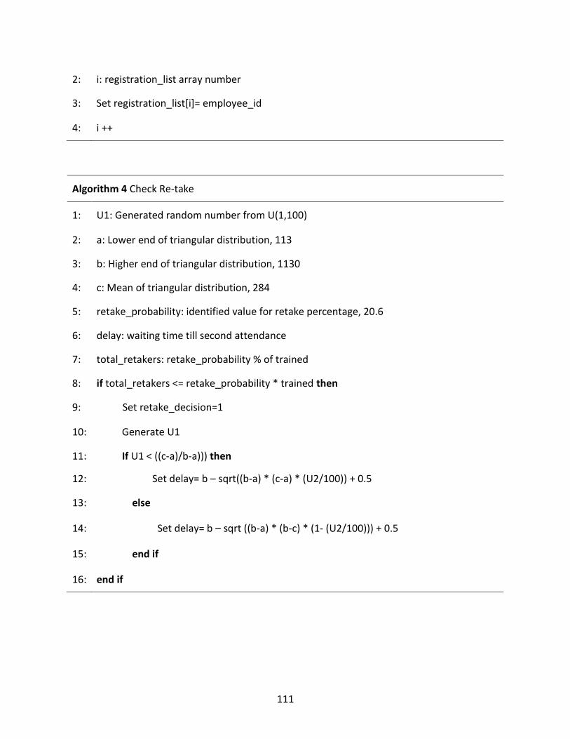
111
2: i: registration_list array number
3: Set registration_list[i]= employee_id
4: i ++
Algorithm 4 Check Re-take
1: U1: Generated random number from U(1,100)
2: a: Lower end of triangular distribution, 113
3: b: Higher end of triangular distribution, 1130
4: c: Mean of triangular distribution, 284
5: retake_probability: identified value for retake percentage, 20.6
6: delay: waiting time till second attendance
7: total_retakers: retake_probability % of trained
8: if total_retakers <= retake_probability * trained then
9: Set retake_decision=1
10: Generate U1
11: If U1 < ((c-a)/b-a))) then
12: Set delay= b – sqrt((b-a) * (c-a) * (U2/100)) + 0.5
13: else
14: Set delay= b – sqrt ((b-a) * (b-c) * (1- (U2/100))) + 0.5
15: end if
16: end if
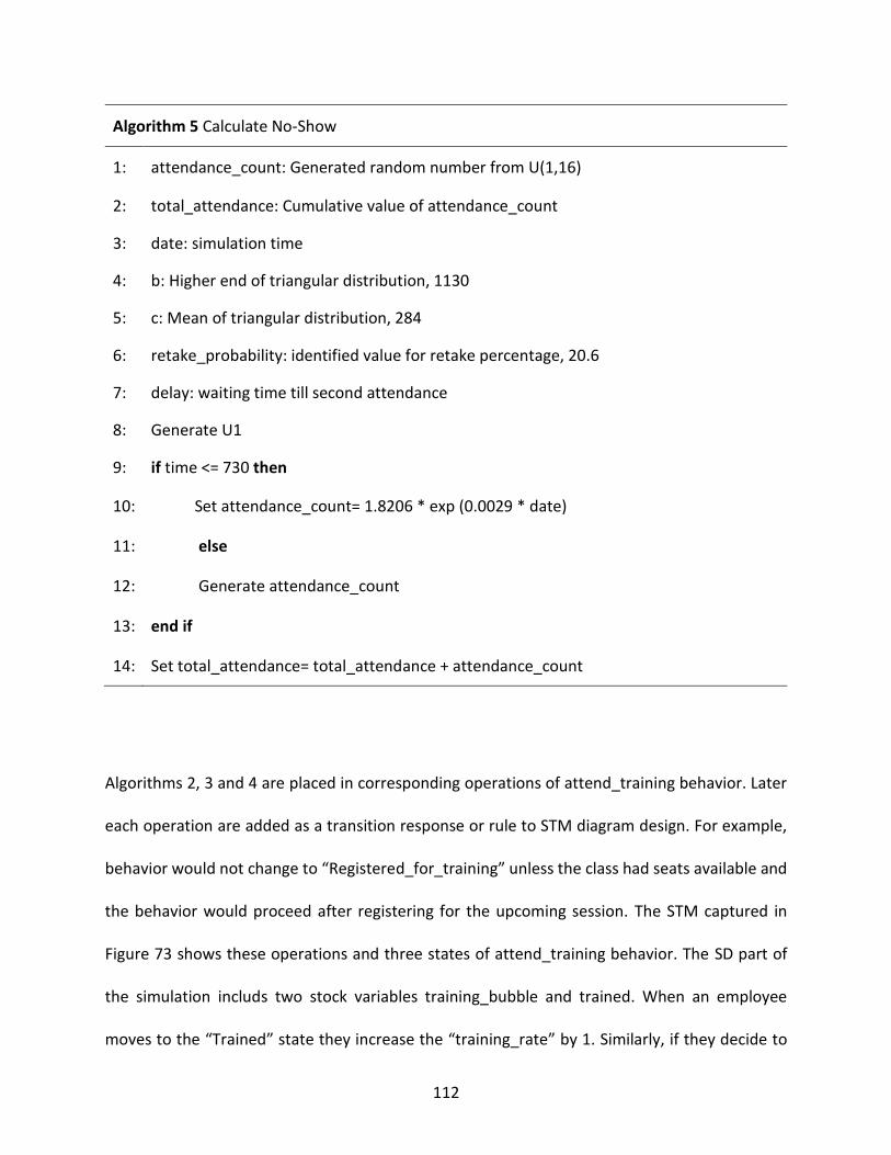
112
Algorithm 5 Calculate No-Show
1: attendance_count: Generated random number from U(1,16)
2: total_attendance: Cumulative value of attendance_count
3: date: simulation time
4: b: Higher end of triangular distribution, 1130
5: c: Mean of triangular distribution, 284
6: retake_probability: identified value for retake percentage, 20.6
7: delay: waiting time till second attendance
8: Generate U1
9: if time <= 730 then
10: Set attendance_count= 1.8206 * exp (0.0029 * date)
11: else
12: Generate attendance_count
13: end if
14: Set total_attendance= total_attendance + attendance_count
Algorithms 2, 3 and 4 are placed in corresponding operations of attend_training behavior. Later
each operation are added as a transition response or rule to STM diagram design. For example,
behavior would not change to “Registered_for_training” unless the class had seats available and
the behavior would proceed after registering for the upcoming session. The STM captured in
Figure 73 shows these operations and three states of attend_training behavior. The SD part of
the simulation includs two stock variables training_bubble and trained. When an employee
moves to the “Trained” state they increase the “training_rate” by 1. Similarly, if they decide to

113
re-take training after waiting for assigned delay duration, they move to “Waiting_training” state,
increasing “return_rate” by 1. Two operations, “get_trained” and “decide_retake”, are
responsible of these actions, respectively.
Figure 73 Attend Training State Diagram
The “train” behavior STM is designed to have two states (Figure 74). When the day, tnow,
matches the date on the imported training schedule, it transitions to “In_training” state. After
waiting 1 day in training, it goes back to waiting state until the next training day. Remaining
algorithm, “Calculate No-Show”, is executed before the training starts on the same day.
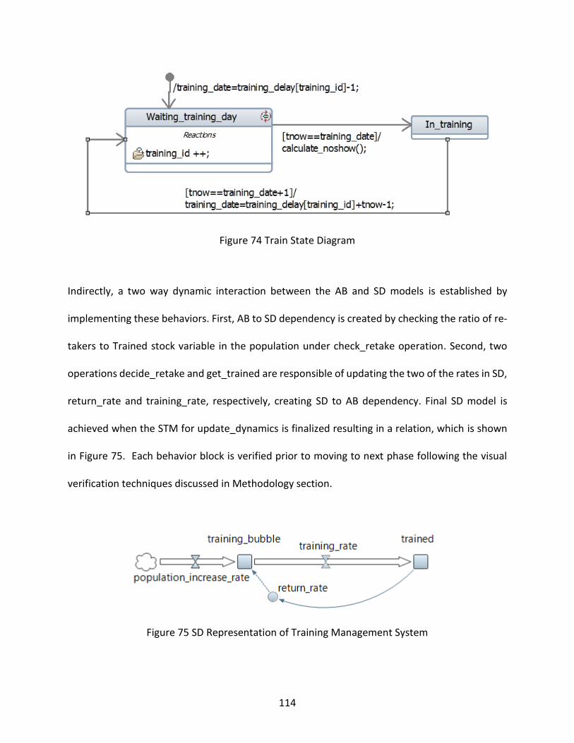
114
Figure 74 Train State Diagram
Indirectly, a two way dynamic interaction between the AB and SD models is established by
implementing these behaviors. First, AB to SD dependency is created by checking the ratio of re-
takers to Trained stock variable in the population under check_retake operation. Second, two
operations decide_retake and get_trained are responsible of updating the two of the rates in SD,
return_rate and training_rate, respectively, creating SD to AB dependency. Final SD model is
achieved when the STM for update_dynamics is finalized resulting in a relation, which is shown
in Figure 75. Each behavior block is verified prior to moving to next phase following the visual
verification techniques discussed in Methodology section.
Figure 75 SD Representation of Training Management System
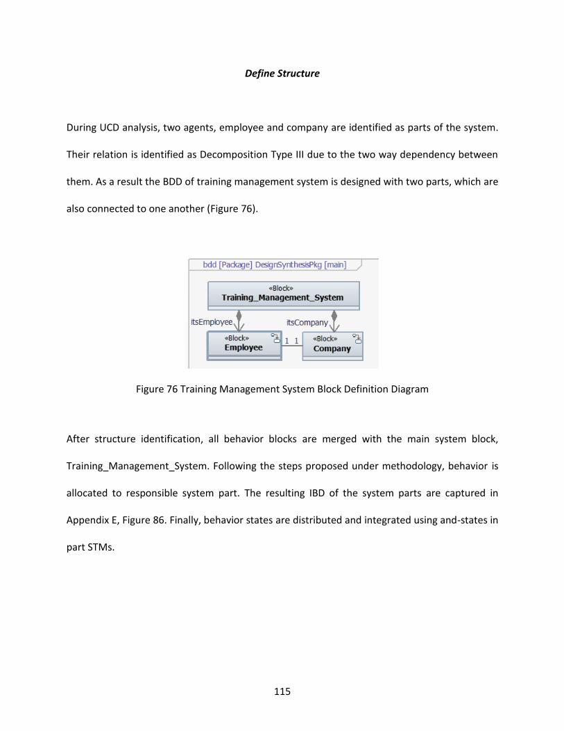
115
Define Structure
During UCD analysis, two agents, employee and company are identified as parts of the system.
Their relation is identified as Decomposition Type III due to the two way dependency between
them. As a result the BDD of training management system is designed with two parts, which are
also connected to one another (Figure 76).
Figure 76 Training Management System Block Definition Diagram
After structure identification, all behavior blocks are merged with the main system block,
Training_Management_System. Following the steps proposed under methodology, behavior is
allocated to responsible system part. The resulting IBD of the system parts are captured in
Appendix E, Figure 86. Finally, behavior states are distributed and integrated using and-states in
part STMs.
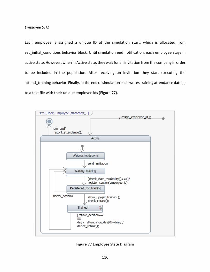
116
Employee STM
Each employee is assigned a unique ID at the simulation start, which is allocated from
set_initial_conditions behavior block. Until simulation end notification, each employee stays in
active state. However, when in Active state, they wait for an invitation from the company in order
to be included in the population. After receiving an invitation they start executing the
attend_training behavior. Finally, at the end of simulation each writes training attendance date(s)
to a text file with their unique employee ids (Figure 77).
Figure 77 Employee State Diagram
117
Company STM
The company is responsible from importing the training schedule at the simulation start which
was allocated from set_initial_conditions behavior block. It remains in Active state until reaching
simulation end time, 1455 days and sends the simulation end event to each employee. When in
Active state, it simultaneously executs three sub-states. First sub-state includes the behavior
from update_time behavior block. At the end of each day, it updates the stock variables and rates
and writes them to a text file with the current day’s number. The second sub-state is responsible
of sending the invitations for the next training to each employee currently in population. The final
sub-state is responsible of running the training operation.
It is important to note the direct relation between input analysis conducted under requirements
analysis section and corresponding behavior allocation. For example, attendance count is studied
using the attendance count data per training and the fit is distributed among the trainings but
not to employees. As a result Calculate No-show operation is allocated to the company and is
used in its STM. The resulting STM is shown in Figure 78.
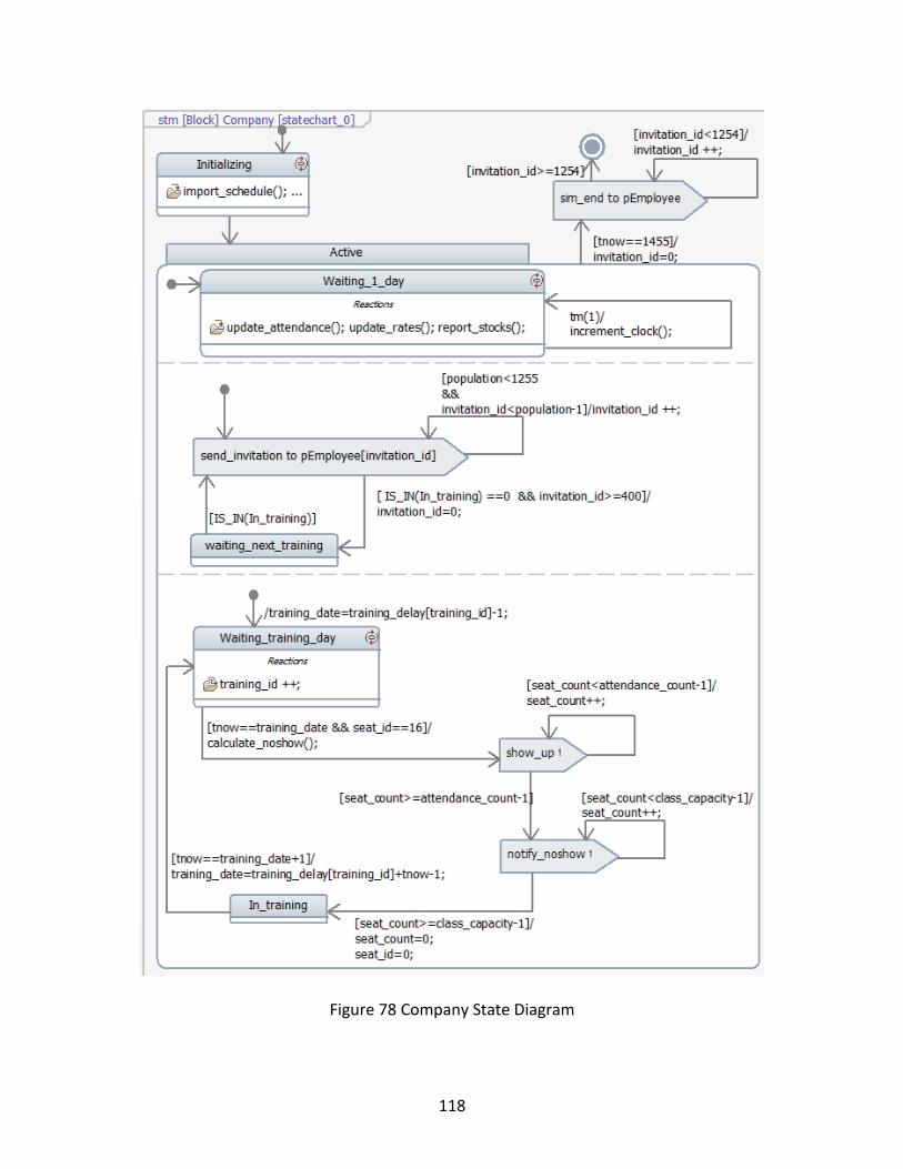
118
Figure 78 Company State Diagram

119
Verify & Validate
Additional to verification completed under behavior design phase, visual and statistical tests are
conducted on the integrated model. First, randomly 10 employees, out of 1255 created, are
selected. Their and company’s simulated statecharts are watched simultaneously for any
potential logic errors. A screenshot capturing this process is shown in Figure 79.
Second, simulated sequence diagram is used with 30 random employees, different from the first
10, with the company to verify the behavior sequence. For example, an agent selected with a
small employee ID is expected to register for a training while some other would be waiting for
training. With the same token, due to population size changes, an agent might not be invited at
all. Figure 80 shows an example of the three cases simulated using a SeqD.

120
Figure 79 Simulated Statecharts
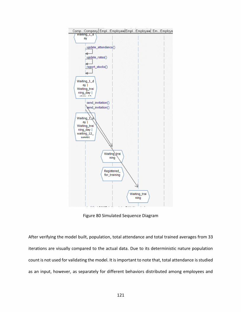
121
Figure 80 Simulated Sequence Diagram
After verifying the model built, population, total attendance and total trained averages from 33
iterations are visually compared to the actual data. Due to its deterministic nature population
count is not used for validating the model. It is important to note that, total attendance is studied
as an input, however, as separately for different behaviors distributed among employees and
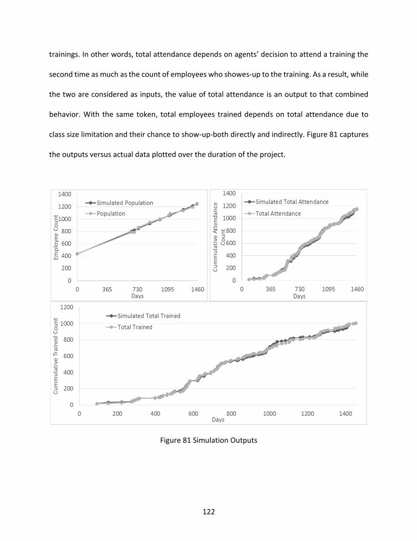
122
trainings. In other words, total attendance depends on agents’ decision to attend a training the
second time as much as the count of employees who showes-up to the training. As a result, while
the two are considered as inputs, the value of total attendance is an output to that combined
behavior. With the same token, total employees trained depends on total attendance due to
class size limitation and their chance to show-up-both directly and indirectly. Figure 81 captures
the outputs versus actual data plotted over the duration of the project.
Figure 81 Simulation Outputs

123
The validity of the model is statistically tested after completing visual checks. Since the input
suggested a non-stationary system, from FYs 09 and 10 to FYs 11 and 12, over a finite time, two
tests are conducted for the two outputs, at the end of FYs 10 and 12 null and alternative
hypotheses tests are;
𝐻0: �̅�(𝑡)𝑟𝑒𝑝𝑙𝑖𝑐𝑎𝑡𝑖𝑜𝑛𝑠 = 𝑋(𝑡)𝑑𝑎𝑡𝑎 𝑎𝑛𝑑 𝐻𝑎: �̅�(𝑡)𝑟𝑒𝑝𝑙𝑖𝑐𝑎𝑡𝑖𝑜𝑛𝑠 ≠ 𝑋(𝑡)𝑑𝑎𝑡𝑎
A table including each replication value at t 730 and 1460 days can be found in APPENDIX D:
SIMULATION OUTPUT. Table 7 captures the actual data collected, average and standard deviation
of the replications, t-test results and t-value at 0.05 significance for 32 degrees of freedom. Each
test value is within the confidence interval. As a result, there is not enough evidence contradicting
the validity of the model and the alternative hypotheses are all rejected.
Table 7 Output Analysis
Total Attendance
FY 10
Total Attendance
FY 12
Total Trained
FY 10
Total Trained
FY 12
Collected Data at t 497 1152 470 1007
Replication Mean 496.879 1147.576 470.636 1005.303
Replication Std. Dev. 3.879 34.710 3.471 33.005
t-test -0.191 -0.732 1.053 -0.295
t-value at 0.025 ± 2.352 ± 2.352 ± 2.352 ± 2.352
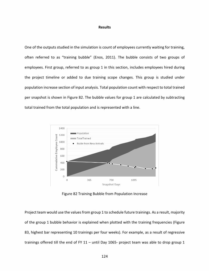
124
Results
One of the outputs studied in the simulation is count of employees currently waiting for training,
often referred to as “training bubble” (Enos, 2011). The bubble consists of two groups of
employees. First group, referred to as group 1 in this section, includes employees hired during
the project timeline or added to due training scope changes. This group is studied under
population increase section of input analysis. Total population count with respect to total trained
per snapshot is shown in Figure 82. The bubble values for group 1 are calculated by subtracting
total trained from the total population and is represented with a line.
Figure 82 Training Bubble from Population Increase
Project team would use the values from group 1 to schedule future trainings. As a result, majority
of the group 1 bubble behavior is explained when plotted with the training frequencies (Figure
83, highest bar representing 10 trainings per four weeks). For example, as a result of regressive
trainings offered till the end of FY 11 – until Day 1065- project team was able to drop group 1

125
bubble almost to half. In FY 12, due to group 1 dropping to 250, the training frequency was
dropped to as low as zero. However, during the first quarter of FY 12 there was an unexplained
increase observed in the group 1 bubble. Furthermore, towards the end of FY 12 - although the
training frequencies were increased - group 1 training rate has continuously decreased. This
resulted in a higher group 1 bubble value compared to end of FY 11.
Figure 83 Group 1 Training Bubble
One of the factors affecting unexpected bubble behavior is the re-takers and it was not accounted
for in training planning. 25.67 % of the employees trained in FYs 09 and 10 had re-attended a
training by the end of FY 12. At the end of FY 12, the ratio of re-takers was 12.59 % of the total
training attendance. However due to the large delay between two attendances, averaging at
500.26 days, this ratio may have increased if data had been collected also for FYs 13 and 14.
Simulated bubble values consists both employees from group 1 and re-takers. Validated model
is used to simulate its change till the end of FY 12. The outputs are plotted using the same graph
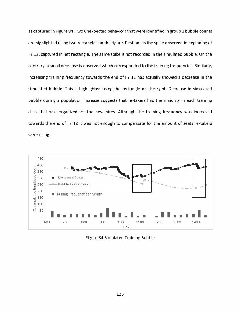
126
as captured in Figure 84. Two unexpected behaviors that were identified in group 1 bubble counts
are highlighted using two rectangles on the figure. First one is the spike observed in beginning of
FY 12, captured in left rectangle. The same spike is not recorded in the simulated bubble. On the
contrary, a small decrease is observed which corresponded to the training frequencies. Similarly,
increasing training frequency towards the end of FY 12 has actually showed a decrease in the
simulated bubble. This is highlighted using the rectangle on the right. Decrease in simulated
bubble during a population increase suggests that re-takers had the majority in each training
class that was organized for the new hires. Although the training frequency was increased
towards the end of FY 12 it was not enough to compensate for the amount of seats re-takers
were using.
Figure 84 Simulated Training Bubble

127
CHAPTER SEVEN: CONCLUSIONS AND FUTURE WORK
This dissertation describes the work on developing a methodology for modeling and simulating
systems with agent-based (AB) and system dynamics (SD) modeling techniques using Systems
Modeling Language (SysML). A methodology is provided, which extends Model-based systems
engineering (MBSE) approach establishes a two way dynamic and continuous communications
within the hybrid platform. Hypothetical and real-world examples are developed on Rational
Rhapsody to demonstrate proposed methodology.
Main challenges in model development can be grouped in four areas. First is the increasing
variation in backgrounds of stakeholders. Every individual or group of individuals adds the know-
how from their perspectives in collaborations. Furthermore, they expect to see how their input-
either previous analysis results or pure data-is integrated into the model and impact the system
outcomes. After input analysis, provided methodology combines findings in two dimensions. First
analysis results are integrated within a behavior. Secondly, they are used for identifying
responsible system components. Resulting system model provides an output of a distributed
behavior composed of integrated inputs. Second challenge is the increasing complexity of
modeled systems. This dissertation provides an approach for managing this complexity and
proposes a technique for identifying and modeling particular behavior and responsibilities of
system parts.
128
The third challenge is more specific to long term projects. It is the need to maintain the coherency
and efficiency of verified and validated models through behavioral and structural change
requests. Proposed approach allows changing, verifying and validating modularized behavior
independently. In other words, an independent behavior block where a change is requested can
be modified, verified and validated and re-allocated to the structural component without
impacting the validity in other behavior blocks.
The final challenge is reusability of modeled behavior. Today, modeling efforts often start from
scratch even if same behavior exists in a previously developed model for a different case by the
same person or group. Provided methodology models behavior and allocates it to a particular
structure. This approach allows modeling the generic behavior rather than the particular case.
Therefore, each behavior block can be separately exported and imported later to be used for a
different case.
Two challenges were faced while working with Rhapsody. First was modeling a behavior, which
follows a probabilistic distribution. An operation implementing random variate generation
technique was added to overcome this limitation. The output from generated variates was
compared to values collected from a simulation software, AnyLogic, and not enough evidence
was found suggesting difference in means. The second challenge was maintaining the simulation
time synchronization between different components of the system. A behavior block was
provided representing a virtual clock that was responsible of updating time within each
component.
129
Additional to its support during model development, provided approach can play an important
role in identifying key factors deriving the system behavior and in providing insight to measures
that can be collected for system evaluation, and analysis. Furthermore, holistic nature of
provided approach allows the proposed methodology to be applicable to different areas of
research. This work demonstrated its application for population dynamics and scheduling
problems. Future applications can include modeling crowd behavior based on geographical
locations. Influenza outbreak modeling can be an example to such application. Furthermore, the
provided method can be extended for hybrid models with alternative configurations. First,
current method’s performance can be evaluated when applied to develop a selected
configuration, such as discrete event simulation and system dynamics combinations. Later, if
necessary, provided steps can be adjusted specifically for each hybrid modeling technique
combinations.

130
APPENDIX A: EXAMPLE MODELS – MOVIE THEATER SEQUENCE DIAGRAM
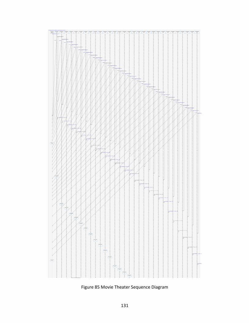
131
Figure 85 Movie Theater Sequence Diagram
sd [Package] watch_movieBBScenariosPkg [Simulated 30-30 All]
itsUc_watch_movie:Uc_watch_movi
e
WaitFor_arrival
ShowMovie
GettingFeedback
OMStartBehaviorEvent()
tm(40) at ROOT.ShowMovie
prtguests[0]:guests
WatchingMovie
GettingRefreshments
WatchingMovie
arrival()
OMStartBehaviorEvent()
gen_uniform(min = 10, max = 30)
tm(11) at ROOT.WatchingMovie
the_end()
tm(5) at ROOT.GettingRefreshments
gen_uniform(min = 10, max = 30)
tm(28) at ROOT.WatchingMovie
prtguests[1]:guests
WatchingMovie
GettingRefreshments
WatchingMovie
arrival()
OMStartBehaviorEvent()
gen_uniform(min = 10, max = 30)
tm(17) at ROOT.WatchingMovie
tm(5) at ROOT.GettingRefreshments
gen_uniform(min = 10, max = 30)
tm(11) at ROOT.WatchingMovie
prtguests[2]:guests
WatchingMovie
GettingRefreshments
WatchingMovie
arrival()OMStartBehaviorEvent()
gen_uniform(min = 10, max = 30)
tm(24) at ROOT.WatchingMovie
tm(5) at ROOT.GettingRefreshments
gen_uniform(min = 10, max = 30)
tm(25) at ROOT.WatchingMovie
prtguests[3]:guests
WatchingMovie
GettingRefreshments
WatchingMovie
arrival() OMStartBehaviorEvent()
gen_uniform(min = 10, max = 30)
tm(10) at ROOT.WatchingMovie
tm(5) at ROOT.GettingRefreshments
gen_uniform(min = 10, max = 30)
tm(17) at ROOT.WatchingMovie
prtguests[4]:guests
WatchingMovie
GettingRefreshments
WatchingMovie
arrival() OMStartBehaviorEvent()
gen_uniform(min = 10, max = 30)
tm(19) at ROOT.WatchingMovie
tm(5) at ROOT.GettingRefreshments
gen_uniform(min = 10, max = 30)
tm(23) at ROOT.WatchingMovie
prtguests[5]:guests
WatchingMovie
GettingRefreshments
WatchingMovie
arrival() OMStartBehaviorEvent()
gen_uniform(min = 10, max = 30)
tm(14) at ROOT.WatchingMovie
tm(5) at ROOT.GettingRefreshments
gen_uniform(min = 10, max = 30)
tm(18) at ROOT.WatchingMovie
prtguests[6]:guests
WatchingMovie
GettingRefreshments
WatchingMovie
arrival() OMStartBehaviorEvent()
gen_uniform(min = 10, max = 30)
tm(28) at ROOT.WatchingMovie
tm(5) at ROOT.GettingRefreshments
gen_uniform(min = 10, max = 30)
tm(16) at ROOT.WatchingMovie
prtguests[7]:guests
WatchingMovie
GettingRefreshments
WatchingMovie
arrival() OMStartBehaviorEvent()
gen_uniform(min = 10, max = 30)
tm(28) at ROOT.WatchingMovie
tm(5) at ROOT.GettingRefreshments
gen_uniform(min = 10, max = 30)
tm(28) at ROOT.WatchingMovie
prtguests[8]:guests
WatchingMovie
GettingRefreshments
WatchingMovie
arrival()OMStartBehaviorEvent()
gen_uniform(min = 10, max = 30)
tm(12) at ROOT.WatchingMovie
tm(5) at ROOT.GettingRefreshments
gen_uniform(min = 10, max = 30)
tm(29) at ROOT.WatchingMovie
prtguests[9]:guests
WatchingMovie
GettingRefreshments
WatchingMovie
arrival()OMStartBehaviorEvent()
gen_uniform(min = 10, max = 30)
tm(14) at ROOT.WatchingMovie
tm(5) at ROOT.GettingRefreshments
gen_uniform(min = 10, max = 30)
tm(14) at ROOT.WatchingMovie
prtguests[10]:guests
WatchingMovie
GettingRefreshments
WatchingMovie
arrival()OMStartBehaviorEvent()
gen_uniform(min = 10, max = 30)
tm(15) at ROOT.WatchingMovie
tm(5) at ROOT.GettingRefreshments
gen_uniform(min = 10, max = 30)
tm(23) at ROOT.WatchingMovie
prtguests[11]:guests
WatchingMovie
GettingRefreshments
WatchingMovie
arrival()OMStartBehaviorEvent()
gen_uniform(min = 10, max = 30)
tm(15) at ROOT.WatchingMovie
tm(5) at ROOT.GettingRefreshments
gen_uniform(min = 10, max = 30)
tm(21) at ROOT.WatchingMovie
prtguests[12]:guests
WatchingMovie
GettingRefreshments
WatchingMovie
arrival()OMStartBehaviorEvent()
gen_uniform(min = 10, max = 30)
tm(11) at ROOT.WatchingMovie
tm(5) at ROOT.GettingRefreshments
gen_uniform(min = 10, max = 30)
tm(19) at ROOT.WatchingMovie
prtguests[13]:guests
WatchingMovie
GettingRefreshments
WatchingMovie
arrival()OMStartBehaviorEvent()
gen_uniform(min = 10, max = 30)
tm(17) at ROOT.WatchingMovie
tm(5) at ROOT.GettingRefreshments
gen_uniform(min = 10, max = 30)
tm(23) at ROOT.WatchingMovie
prtguests[14]:guests
WatchingMovie
GettingRefreshments
WatchingMovie
arrival()OMStartBehaviorEvent()
gen_uniform(min = 10, max = 30)
tm(11) at ROOT.WatchingMovie
tm(5) at ROOT.GettingRefreshments
gen_uniform(min = 10, max = 30)
tm(13) at ROOT.WatchingMovie
prtguests[15]:guests
WatchingMovie
GettingRefreshments
WatchingMovie
arrival()OMStartBehaviorEvent()
gen_uniform(min = 10, max = 30)
tm(21) at ROOT.WatchingMovie
tm(5) at ROOT.GettingRefreshments
gen_uniform(min = 10, max = 30)
tm(12) at ROOT.WatchingMovie
prtguests[16]:guests
WatchingMovie
GettingRefreshments
WatchingMovie
arrival()OMStartBehaviorEvent()
gen_uniform(min = 10, max = 30)
tm(25) at ROOT.WatchingMovie
tm(5) at ROOT.GettingRefreshments
gen_uniform(min = 10, max = 30)
tm(29) at ROOT.WatchingMovie
prtguests[17]:guests
WatchingMovie
GettingRefreshments
WatchingMovie
arrival()OMStartBehaviorEvent()
gen_uniform(min = 10, max = 30)
tm(12) at ROOT.WatchingMovie
tm(5) at ROOT.GettingRefreshments
gen_uniform(min = 10, max = 30)
tm(27) at ROOT.WatchingMovie
prtguests[18]:guests
WatchingMovie
GettingRefreshments
WatchingMovie
arrival()OMStartBehaviorEvent()
gen_uniform(min = 10, max = 30)
tm(17) at ROOT.WatchingMovie
tm(5) at ROOT.GettingRefreshments
gen_uniform(min = 10, max = 30)
tm(14) at ROOT.WatchingMovie
prtguests[19]:guests
WatchingMovie
GettingRefreshments
WatchingMovie
arrival()OMStartBehaviorEvent()
gen_uniform(min = 10, max = 30)
tm(26) at ROOT.WatchingMovie
tm(5) at ROOT.GettingRefreshments
gen_uniform(min = 10, max = 30)
tm(22) at ROOT.WatchingMovie
prtguests[20]:guests
WatchingMovie
GettingRefreshments
WatchingMovie
arrival()OMStartBehaviorEvent()
gen_uniform(min = 10, max = 30)
tm(21) at ROOT.WatchingMovie
tm(5) at ROOT.GettingRefreshments
gen_uniform(min = 10, max = 30)
tm(21) at ROOT.WatchingMovie
prtguests[21]:guests
WatchingMovie
GettingRefreshments
WatchingMovie
arrival()OMStartBehaviorEvent()
gen_uniform(min = 10, max = 30)
tm(14) at ROOT.WatchingMovie
tm(5) at ROOT.GettingRefreshments
gen_uniform(min = 10, max = 30)
tm(17) at ROOT.WatchingMovie
prtguests[22]:guests
WatchingMovie
GettingRefreshments
WatchingMovie
arrival()OMStartBehaviorEvent()
gen_uniform(min = 10, max = 30)
tm(12) at ROOT.WatchingMovie
tm(5) at ROOT.GettingRefreshments
gen_uniform(min = 10, max = 30)
tm(27) at ROOT.WatchingMovie
prtguests[23]:guests
WatchingMovie
GettingRefreshments
WatchingMovie
arrival()OMStartBehaviorEvent()
gen_uniform(min = 10, max = 30)
tm(23) at ROOT.WatchingMovie
tm(5) at ROOT.GettingRefreshments
gen_uniform(min = 10, max = 30)
tm(24) at ROOT.WatchingMovie
prtguests[24]:guests
WatchingMovie
GettingRefreshments
WatchingMovie
arrival()OMStartBehaviorEvent()
gen_uniform(min = 10, max = 30)
tm(22) at ROOT.WatchingMovie
tm(5) at ROOT.GettingRefreshments
gen_uniform(min = 10, max = 30)
tm(13) at ROOT.WatchingMovie
prtguests[25]:guests
GettingRefreshments
WatchingMovie
arrival()OMStartBehaviorEvent()
gen_uniform(min = 10, max = 30)
tm(12) at ROOT.WatchingMovie
tm(5) at ROOT.GettingRefreshments
gen_uniform(min = 10, max = 30)
tm(12) at ROOT.WatchingMovie
prtguests[26]:guests
GettingRefreshments
WatchingMovie
arrival()OMStartBehaviorEvent()
gen_uniform(min = 10, max = 30)
tm(11) at ROOT.WatchingMovie
tm(5) at ROOT.GettingRefreshments
gen_uniform(min = 10, max = 30)
tm(11) at ROOT.WatchingMovie
prtguests[27]:guests
WatchingMovie
GettingRefreshments
WatchingMovie
arrival()OMStartBehaviorEvent()
gen_uniform(min = 10, max = 30)
tm(26) at ROOT.WatchingMovie
tm(5) at ROOT.GettingRefreshments
gen_uniform(min = 10, max = 30)
tm(19) at ROOT.WatchingMovie
prtguests[28]:guests
WatchingMovie
GettingRefreshments
WatchingMovie
arrival()OMStartBehaviorEvent()
gen_uniform(min = 10, max = 30)
tm(28) at ROOT.WatchingMovie
tm(5) at ROOT.GettingRefreshments
gen_uniform(min = 10, max = 30)
tm(21) at ROOT.WatchingMovie
prtguests[29]:guests
WatchingMovie
GettingRefreshments
WatchingMovie
arrival()OMStartBehaviorEvent()
gen_uniform(min = 10, max = 30)
tm(25) at ROOT.WatchingMovie
tm(5) at ROOT.GettingRefreshments
gen_uniform(min = 10, max = 30)
tm(17) at ROOT.WatchingMovie

132
APPENDIX B: EXPONENTIAL VARIATE DATE

133
Table 8 Generated Date Frequency
Days
AnyLogic Rhapsody
Days
AnyLogic Rhapsody
Transitioning Agent Count Transitioning Agent Count
0 0 0 26 46 45
1 5 7 27 48 46
2 8 10 28 48 47
3 11 14 29 48 47
4 16 20 30 48 48
5 21 22 31 48 48
6 25 24 32 48 49
7 28 25 33 48 49
8 31 29 34 48 49
9 33 30 35 48 49
10 34 34 36 49 49
11 35 34 37 49 49
12 36 36 38 49 49
13 36 38 39 49 50
14 37 39 40 49 50
15 38 40 41 49 50
16 41 41 42 49 50
17 41 42 43 49 50
18 42 42 44 49 50
19 44 42 45 49 50
20 44 45 46 49 50
21 45 45 47 49 50
22 45 45 48 50 50
23 45 45 49 50 50
24 46 45 50 50 50
25 46 45

134
APPENDIX C: TRAINING SCHEDULE

135
Table 9 Training Dates and Attendance Counts
Training
Date
# of
Employees
Training
Date
# of
Employees
Training
Date
# of
Employees
Training
Date
# of
Employees
1/1/2009 16 5/3/2010 16 5/2/2011 3 2/27/2012 3
3/3/2009 3 5/5/2010 16 5/9/2011 11 3/5/2012 16
5/12/2009 5 6/14/2010 13 5/20/2011 5 3/12/2012 16
6/30/2009 13 6/16/2010 13 5/31/2011 8 3/19/2012 9
7/7/2009 1 6/21/2010 13 6/6/2011 4 3/20/2012 9
7/8/2009 5 6/23/2010 15 6/8/2011 11 3/21/2012 10
7/10/2009 7 6/28/2010 10 6/9/2011 6 3/27/2012 11
7/16/2009 5 7/19/2010 10 6/11/2011 2 4/9/2012 9
7/22/2009 2 7/21/2010 11 6/13/2011 6 4/16/2012 11
7/23/2009 5 7/26/2010 9 6/14/2011 5 4/30/2012 7
7/30/2009 7 8/23/2010 8 6/16/2011 11 6/4/2012 10
8/5/2009 3 8/25/2010 11 6/22/2011 1 6/5/2012 12
8/6/2009 4 9/8/2010 11 6/25/2011 6 6/18/2012 12
8/12/2009 6 9/13/2010 11 6/27/2011 1 6/25/2012 3
11/4/2009 1 9/23/2010 13 6/28/2011 4 6/29/2012 7
11/23/2009 7 9/27/2010 12 7/1/2011 1 7/16/2012 3
12/1/2009 3 9/30/2010 11 7/11/2011 14 7/19/2012 1
12/3/2009 3 10/4/2010 14 7/13/2011 2 7/30/2012 9
12/14/2009 8 10/6/2010 11 7/18/2011 11 8/6/2012 5
12/16/2009 11 10/11/2010 9 7/20/2011 2 8/7/2012 7
1/5/2010 9 10/14/2010 6 7/21/2011 5 8/8/2012 5
1/7/2010 9 10/18/2010 4 8/3/2011 6 8/13/2012 8
1/25/2010 1 11/1/2010 11 8/4/2011 13 8/14/2012 4
2/1/2010 7 11/8/2010 10 8/5/2011 14 8/15/2012 5
2/4/2010 7 11/11/2010 10 8/8/2011 1 8/21/2012 3
2/8/2010 7 12/1/2010 10 8/30/2011 13 9/11/2012 5
2/15/2010 3 12/8/2010 9 9/20/2011 8 9/24/2012 7
3/15/2010 1 1/10/2011 11 10/10/2011 13 2/27/2012 3
3/29/2010 12 1/13/2011 6 10/11/2011 9 3/5/2012 16
3/31/2010 8 1/17/2011 5 10/12/2011 11 3/12/2012 16
4/6/2010 12 2/7/2011 11 10/13/2011 5 3/19/2012 9
4/8/2010 16 2/10/2011 1 10/18/2011 12 3/20/2012 9
4/12/2010 9 2/14/2011 10 11/1/2011 2 3/21/2012 10
4/14/2010 9 2/21/2011 7 11/11/2011 1 3/27/2012 11
4/19/2010 12 2/28/2011 8 12/6/2011 2 4/9/2012 9
4/20/2010 9 3/14/2011 3 12/19/2011 9 4/16/2012 11
4/22/2010 9 3/27/2011 10 1/24/2012 10 4/30/2012 7
4/27/2010 15 4/4/2011 13 2/16/2012 2 6/4/2012 10
4/29/2010 12 4/8/2011 1 2/21/2012 11 6/5/2012 12

136
APPENDIX D: SIMULATION OUTPUT

137
Table 10 Simulation Results per Replication
Total Attendance FY 10
Total Attendance FY 12
Total Trained FY 10
Total Trained FY 12
Replication 1 503 1142 468 1009
Replication 2 499 1169 469 1031
Replication 3 503 1151 469 1009
Replication 4 498 1106 469 967
Replication 5 502 1168 467 1027
Replication 6 490 1135 468 999
Replication 7 490 1182 468 1037
Replication 8 495 1172 470 1032
Replication 9 500 1130 464 993
Replication 10 503 1198 466 1052
Replication 11 497 1136 468 999
Replication 12 501 1103 468 959
Replication 13 495 1042 470 909
Replication 14 503 1118 470 970
Replication 15 496 1196 466 1051
Replication 16 495 1117 471 971
Replication 17 497 1163 470 1018
Replication 18 496 1153 471 1007
Replication 19 499 1150 470 1009
Replication 20 495 1154 475 1009
Replication 21 493 1195 478 1047
Replication 22 497 1160 478 1012
Replication 23 497 1138 476 993
Replication 24 496 1146 476 999
Replication 25 498 1131 472 989
Replication 26 493 1206 473 1063
Replication 27 493 1082 472 943
Replication 28 493 1181 471 1034
Replication 29 497 1120 475 978
Replication 30 497 1144 468 1000
Replication 31 503 1163 470 1018
Replication 32 491 1175 470 1033
Replication 33 492 1144 475 1008

138
APPENDIX E: TRAINING MANAGEMENT SYSTEM INTERNAL BLOCK DIAGRAM
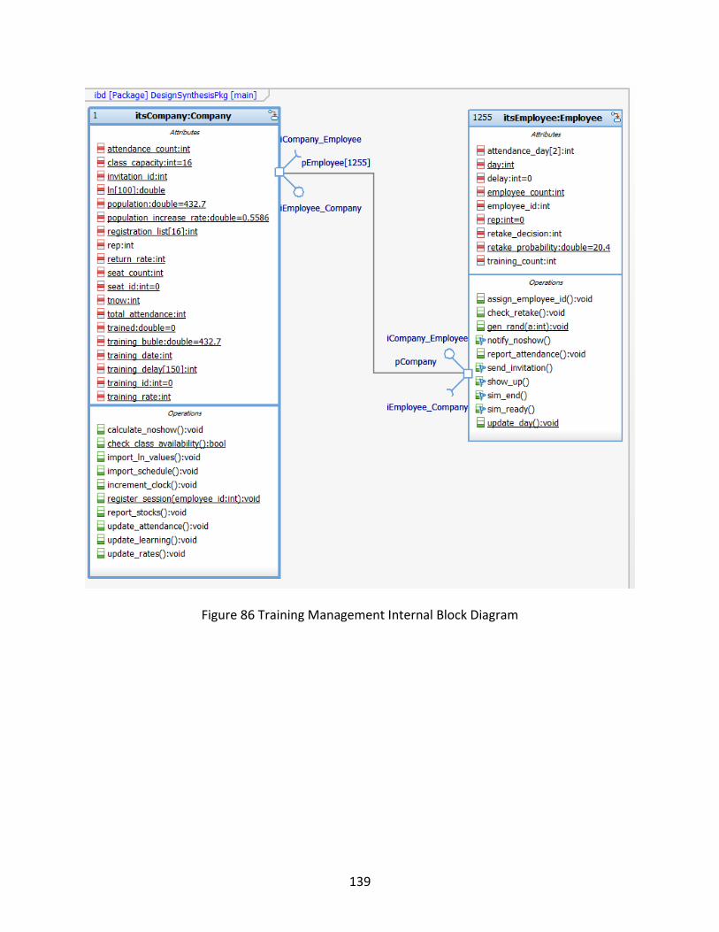
139
Figure 86 Training Management Internal Block Diagram

140
APPENDIX F: ATTENDANCE COUNT REGRESSION ANALYSIS
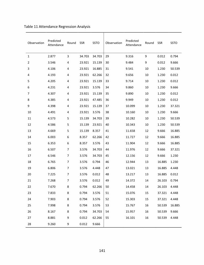
141
Table 11 Attendance Regression Analysis
Observation Predicted Attendance
Round SSR SSTO Observation Predicted Attendance
Round SSR SSTO
1 2.877 3 34.703 34.703 29 9.316 9 0.012 0.794
2 3.546 4 23.921 15.139 30 9.484 9 0.012 9.666
3 4.106 4 23.921 16.885 31 9.541 10 1.230 50.539
4 4.193 4 23.921 62.266 32 9.656 10 1.230 0.012
5 4.205 4 23.921 15.139 33 9.714 10 1.230 0.012
6 4.231 4 23.921 3.576 34 9.860 10 1.230 9.666
7 4.307 4 23.921 15.139 35 9.890 10 1.230 0.012
8 4.385 4 23.921 47.485 36 9.949 10 1.230 0.012
9 4.398 4 23.921 15.139 37 10.099 10 1.230 37.321
10 4.491 4 23.921 3.576 38 10.160 10 1.230 9.666
11 4.573 5 15.139 34.703 39 10.282 10 1.230 50.539
12 4.586 5 15.139 23.921 40 10.343 10 1.230 50.539
13 4.669 5 15.139 8.357 41 11.658 12 9.666 16.885
14 6.003 6 8.357 62.266 42 11.727 12 9.666 16.885
15 6.353 6 8.357 3.576 43 11.904 12 9.666 16.885
16 6.507 7 3.576 34.703 44 11.976 12 9.666 37.321
17 6.546 7 3.576 34.703 45 12.156 12 9.666 1.230
18 6.765 7 3.576 0.794 46 12.944 13 16.885 1.230
19 6.806 7 3.576 4.448 47 13.021 13 16.885 4.448
20 7.225 7 3.576 0.012 48 13.217 13 16.885 0.012
21 7.268 7 3.576 0.012 49 14.372 14 26.103 0.794
22 7.670 8 0.794 62.266 50 14.458 14 26.103 4.448
23 7.833 8 0.794 3.576 51 15.076 15 37.321 4.448
24 7.903 8 0.794 3.576 52 15.303 15 37.321 4.448
25 7.998 8 0.794 3.576 53 15.767 16 50.539 16.885
26 8.167 8 0.794 34.703 54 15.957 16 50.539 9.666
27 8.881 9 0.012 62.266 55 16.101 16 50.539 4.448
28 9.260 9 0.012 9.666

142
LIST OF REFERENCES
Akbas, M. I., Brust, M. R., Ribeiro, C. H. C., & Turgut, D. (2015). A Preferential Attachment Model
for Primate Social Networks. Elsevier Computer Networks Journal, 76(0), 207–226.
Akkermans, H. (2001). Emergent Supply Networks :System Dynamics Simulation of Adaptive
Supply Agents. In Proceedings of the 34th Hawaii International Conference on System
Sciences (Vol. 9, pp. 1–11).
Barlas, Y. (1996). Formal aspects of model validity and validation in system dynamics. System
Dynamics Review, 12(3), 183–210. http://doi.org/10.1002/(SICI)1099-
1727(199623)12:3<183::AID-SDR103>3.0.CO;2-4
Basole, R. C., & Bodner, D. A. (2015). Computational Modeling of Complex Enterprise Systems: A
Multi-Level Approach. In Modeling and Simulation in the Systems Engineering Life Cycle,
Simulation Foundations, Methods and Applications (M. L. Lope, p. 369). Liverpool: Springer-
Verlag. http://doi.org/10.1007/978-1-4471-5634-5_10
Bersini, H. (2012). UML for ABM. Journal of Artificial Societies and Social Simulation, 15(1).
Retrieved from http://jasss.soc.surrey.ac.uk/15/1/9.html
Borshchev, A., & Filippov, A. (2004). From System Dynamics to Agent Based Modeling: Reasons,
Techniques, Tools. In The 22nd International Conference of the System Dynamics Society.
Oxford.
Cellier, F. E. (1991). Population Dynamics Modeling. In Continuous System Modeling (pp. 417–
454). Springer New York. http://doi.org/10.1007/978-1-4757-3922-0_10
Chaim, R. (2008). Pension Funds Governance: Combining SD, Agent Based Modelling and Fuzzy
Logic to Adress Dynamic Asset and Liability Management (ALM) Problem. In Proceedings of
the 26th International Conference of the System Dynamics Society. Retrieved from
http://www.systemdynamics.org/conferences/2008/proceed/proceed.pdf
Collins, A., Petty, M., Vernon-Bido, D., & Sherfey, S. (2015). A Call to Arms: Standards for Agent-
Based Modeling and Simulation. Journal of Artificial Societies & Social Simulation, 18(3), 1.
Retrieved from
http://eds.b.ebscohost.com.ezproxy.net.ucf.edu/abstract?site=eds&scope=site&jrnl=1460
7425&AN=103679390&h=gmGecMSG8jSSoPuiDarsmhaS7KOXSJFaX80r+MEf+TbT36O7PD6
143
WPfTXWvJ/7JrwkBkAYnBzpUkyTKP4JmS2zw==&crl=c&resultLocal=ErrCrlNoResults&result
Ns=Ehost&cr
Coyle, R. G. (2001a). System Dynamics Modeling (2nd ed.). Boca Raton: Chapman and Hall/CRC.
Coyle, R. G. (2001b). System Dynamics Modeling (2nd ed.). Boca Raton: Chapman and Hall/CRC.
David, P., Idasiak, V., & Kratz, F. (2010). Reliability study of complex physical systems using SysML.
Reliability Engineering & System Safety, 95(4), 431–450.
http://doi.org/10.1016/j.ress.2009.11.015
Enos, J. R. (2011). Dynamics of Combat Aviator Training. In Proceedings of the 29th International
Conference of the System Dynamics Society (pp. 1–15).
Figueredo, G. P., & Aickelin, U. (2011). Comparing System Dynamics and Agent-Based Simulation
for Tumour Growth and its Interactions with Effector Cells. In Proceedings of the 2011
Summer Computer Simulation Conference (pp. 52–59). Retrieved from
http://arxiv.org/abs/1108.3235
Friedenthal, S., Moore, A., & Steiner, R. (2009). A practical guide to SysML. Burlington, MA:
Elsevier Inc.
Gaube, V., Kaiser, C., Wildenberg, M., Adensam, H., Fleissner, P., Kobler, J., … Haberl, H. (2009).
Combining agent-based and stock-flow modelling approaches in a participative analysis of
the integrated land system in Reichraming, Austria. Landscape Ecology, 24(9), 1149–1165.
http://doi.org/10.1007/s10980-009-9356-6
GCF. (2014). Giraffe Conservation Foundation. Retrieved May 28, 2015, from
http://www.giraffeconservation.org/
Gilbert, N., & Bankes, S. (2002). Platforms and Methods for Agent-Based Modeling. Proceedings
of the National Academy of Sciences of the United States of America, 99(3), 7197–7198.
http://doi.org/10.1073/pnas.072079499
Gilli, Q., Mustapha, K., Frayret, J., Lahrichi, N., & Karimi, E. (2014). Agent-Based Simulation of
Colorectal Cancer Care Trajectory: Patient Model. Cirrelt, 67(December), 1–40. Retrieved
from https://www.cirrelt.ca/DocumentsTravail/CIRRELT-2014-67.pdf
Größler, A., Stotz, M., & Schieritz, N. (2003). A Software Interface Between System Dynamics and
Agent-Based Simulations – Linking Vensim ® and RePast ®. In Proceedings of the 21st System
Dynamics Society International Conference. New York.
Haghani, A., Lee, S. Y., & Byun, J. H. (2003). A System Dynamics Approach to Land Use /
Transportation System Performance Modeling. Journal of Advanced Transportation, 37(1),

144
1–41. http://doi.org/10.1002/atr.5670370103
Hause, M. (2006). The SysML Modelling Language. In Proceedings of Fifteenth European Systems
Engineering Conference.
Hoffmann, H.-P. (2014). IBM Rational Harmony Deskbook. Retrieved from
https://www.ibm.com/developerworks/community/groups/service/html/communityview
?communityUuid=dbc39547-3619-4c31-9535-
0b583a4e6190#fullpageWidgetId=W62078615f88f_4809_afad_c27cdc9d7e71&file=2132d
88d-4dde-40b4-8102-254ca4456c82
Homer, J. B., & Hirsch, G. B. (2006). System dynamics modeling for public health: background and
opportunities. American Journal of Public Health, 96(3), 452–8.
http://doi.org/10.2105/AJPH.2005.062059
Huang, E., Ramamurthy, R., & Mcginnis, L. F. (2007). System and simulation modeling using
SySML. In Proceedings of the 2007 Winter Simulation Conference (pp. 796–803).
Huntsville, U. of A. (2014). Euler’s Numerical Method. Retrieved January 1, 2014, from
http://howellkb.uah.edu//DEtext/Part2/Euler_Method.pdf
IBM. (2014). IBM Rational Rhapsody 8.1.1 Documentation. Retrieved from
http://127.0.0.1:50992/help/index.jsp?nav=%2F1
INCOSE. (2011). Vee-Model. INCOSE. Retrieved from
http://www.incose.org/chesapek/mailings/2011/2011_02_Mailing.html
Jahangirian, M., Eldabi, T., Naseer, A., Stergioulas, L. K., & Young, T. (2010). Simulation in
manufacturing and business: A review. European Journal of Operational Research, 203(1),
1–13. http://doi.org/10.1016/j.ejor.2009.06.004
Johnson, T. A., Jobe, J. M., Paredis, C. J. J., & Burkhart, R. (2007). Modeling continuous system
dynamics in sysml. In IMECE 2007 (pp. 1–9). Seattle, Washington, USA.
Johnson, T. A., Paredis, C. J. J., & Burkhart, R. (2011). Integrating models and simulations of
continuous dynamics into SysML. Journal of Computing and Information Science in
Engineering, 12(1), 1–11. http://doi.org/10.1115/1.4005452
Lättilä, L., Hilletofth, P., & Lin, B. (2010). Hybrid simulation models – When, Why, How? Expert
Systems with Applications, 37(12), 7969–7975. http://doi.org/10.1016/j.eswa.2010.04.039
Lukens, S., Depasse, J., Rosenfeld, R., Ghedin, E., Mochan, E., Brown, S. T., … Clermont, G. (2014).
A Large-Scale Immuno-Epidemiological Simulation of Influenza A Epidemics. BMC Public
Health, 14(1019).
145
Macal, C. M., & North, M. J. (2007). Agent-Based Modeling and Simulation: Desktop ABMS. In
Winter Simulation Conference (pp. 95–106). IEEE.
Macal, C. M., & North, M. J. (2010). Tutorial on agent-based modelling and simulation. Journal of
Simulation, 4(3), 151–162. http://doi.org/10.1057/jos.2010.3
Masad, D., & Kazil, J. (2015). Mesa : An Agent-Based Modeling Framework. In 14th PYTHON in
Science Conference (pp. 53–60).
Mcginnis, L., & Ustun, V. (2009). A simple example of SysML-driven simulation. In Proceedings of
the 2009 Winter Simulation Conference (pp. 1703–1710).
OMG. (2007). OMG Systems Modeling Language. Retrieved 08 2012, from
http://www.omgsysml.org/
Pastrana, J. (2014). Model-Based Systems Engineering (MSBE) Approach to Distributed and Hybrid
Simulation Systems. University of Central Florida.
Phelan, S. E. (1999). A note on the correspondence between complexity and system theory.
Systemic Practice and Action Research, 12(3), 237–246.
Pourdehnad, J., Maani, K., & Sedehi, H. (2002). System Dynamics and Intelligent Agent-Based
Simulation : Where is the Synergy ? In 20th International Conference of the System Dynamics
Society. Polermo.
Ramos, A. L., Ferreira, J. V., & Barcelo, J. (2012). Model-based systems engineering : An emerging
approach for modern systems. IEEE Transactions on Systems, Man, and Cybernetics - Part C:
Applications and Reviews, 42(1), 101–111.
Scholl, H. J. (2001). Agent Based and System Dynamics Modeling: A Call for Cross Study and Joint
Research. Proceedings of the 34th Annual Hawaii International Conference on System
Sciences, 3, 8. http://doi.org/10.1109/HICSS.2001.926296
Sellgren, U., Törngren, M., Malvius, D., & Biehl, M. (2009). Product lifecycle management for
mechatronics integration. In International Conference on Product Lifecycle Management
(pp. 1–11).
Silhavy, R., Silhavy, P., & Prokopova, Z. (2011). Behavioral Modeling in System Engineering. In
Proceedings of the 13th WSEAS International Conference on Automatic Control, Modelling
& Simulation (pp. 100–105).
Soyler Akbas, A., Mykoniatis, K., Angelopoulou, A., & Karwowski, W. (2014). A Model-based
Approach to Modeling a Hybrid Simulation Platform. In Proceedings of the Symposium on
Theory of Modeling & Simulation (pp. 31:1–31:6). Tampa: Society for Computer Simulation
146
International.
Sterman, J. D. (1992). System Dynamics Modeling for Project Management. Cambridge. Retrieved
from http://scripts.mit.edu/~jsterman/docs/Sterman-1992-SystemDynamicsModeling.pdf
Swinerd, C., & McNaught, K. R. (2012). Design classes for hybrid simulations involving agent-
based and system dynamics models. Simulation Modelling Practice and Theory, 25, 118–
133. http://doi.org/10.1016/j.simpat.2011.09.002
The Pennsylvania State University. (2015). The Coefficient of Determination. Retrieved
September 30, 2015, from https://onlinecourses.science.psu.edu/stat501/node/255
Towill, D. R. (1993). System Dynamics-Background, Methodology and Applications. Computing &
Control Engineering Journal, 4(5), 201. Retrieved from
http://ieeexplore.ieee.org/xpls/abs_all.jsp?arnumber=242110
UA. (2015). Autocorrelation. Retrieved from http://www.ltrr.arizona.edu/~dmeko/notes_3.pdf
Weilkiens, T. (2006). Systems Engineering with SysML/UML. Burlington, MA: Morgan Kaufmann
Publishers.